Partial Fractions - Lecture 7: The Partial Fraction...
27
Partial Fractions Matthew M. Peet Illinois Institute of Technology Lecture 7: The Partial Fraction Expansion
Transcript of Partial Fractions - Lecture 7: The Partial Fraction...

Partial Fractions
Matthew M. PeetIllinois Institute of Technology
Lecture 7: The Partial Fraction Expansion

Introduction
In this Lecture, you will learn: The Inverse Laplace Transform
• Simple Forms
The Partial Fraction Expansion
• How poles relate to dominant modes
• Expansion using single poles
• Repeated Poles
• Complex Pairs of PolesI Inverse Laplace
M. Peet Lecture 7: Control Systems 2 / 27

Recall: The Inverse Laplace Transform of a Signal
To go from a frequency domain signal, u(s), to the time-domain signal, u(t), weuse the Inverse Laplace Transform.
Definition 1.
The Inverse Laplace Transform of a signal u(s) is denoted u(t) = Λ−1u.
u(t) = Λ−1u =
∫ ∞0
eıωtu(ıω)dω
• Like Λ, the inverse Laplace Transform Λ−1 is also a Linear system.
• Identity: Λ−1Λu = u.
• Calculating the Inverse Laplace Transform can be tricky. e.g.
y =s3 + s2 + 2s− 1
s4 + 3s3 − 2s2 + s + 1
M. Peet Lecture 7: Control Systems 3 / 27

Poles and Rational Functions
Definition 2.
A Rational Function is the ratio of two polynomials:
u(s) =n(s)
d(s)
Most transfer functions are rational.
Definition 3.
The point sp is a Pole of the rational function u(s) = n(s)d(s) if d(sp) = 0.
• It is convenient to write a rational function using its poles
n(s)
d(s)=
n(s)
(s− p1)(s− p2) · · · (s− pn)
• The Inverse Laplace Transform of an isolated pole is easy:
u(s) =1
s + pmeans u(t) = e−pt
M. Peet Lecture 7: Control Systems 4 / 27

Partial Fraction Expansion
Definition 4.
The Degree of a polynomial n(s), is the highest power of s with a nonzerocoefficient.
Example: The degree of n(s) is 4
n(s) = s4 + .5s2 + 1
Definition 5.
A rational function u(s) = n(s)d(s) is Strictly Proper if the degree of n(s) is less
than the degree of d(s).
• We assume that n(s) has lower degree than d(s)
• Otherwise, perform long division until we have a strictly proper remainder
s3 + 2s2 + 6s + 7
s2 + s + 5= s + 1 +
2
s2 + s + 5
M. Peet Lecture 7: Control Systems 5 / 27
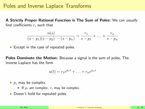
Poles and Inverse Laplace Transforms
A Strictly Proper Rational Function is The Sum of Poles: We can usuallyfind coefficients ri such that
n(s)
(s− p1)(s− p2) · · · (s− pn)=
r1s− p1
+ . . . +rn
s− pn
• Except in the case of repeated poles.
Poles Dominate the Motion: Because a signal is the sum of poles, Theinverse Laplace has the form
u(t) = r1ep1t + . . . + rne
pnt
• pi may be complex.I If pi are complex, ri may be complex.
• Doesn’t hold for repeated poles.
M. Peet Lecture 7: Control Systems 6 / 27

Examples
Simple State-Space: Step Response
y(s) =s− 1
(s + 1)s=
2
s + 1− 1
s
y(t) = e−t − 1
21(t)
Suspension System: Impulse Response
y(s) =1
J
1
s2 − Mgl2J
=1
J
√2J
Mgl
1
s−√
Mgl2J
− 1
s +√
Mgl2J
y(t) =
1
J
√2J
Mgl
(e√
Mgl2J t − e−
√Mgl2J t)
Simple State-Space: Sinusoid Response
y(s) =s− 1
(s + 1)(s2 + 1)=
(s
s2 + 1− 1
s + 1
)y(t) =
1
2cos t− 1
2e−t
M. Peet Lecture 7: Control Systems 7 / 27

Partial Fraction Expansion
Conclusion: If we can find coefficients ri such that
u(s) =n(s)
d(s)=
n(s)
(s− p1)(s− p2) · · · (s− pn)
=r1
s− p1+ · · ·+ rn
s− pn,
then this is the PARTIAL FRACTION EXPANSION of u(s).
We will address several cases of increasing complexity:
1. d(s) has all real, non-repeating roots.
2. d(s) has all real roots, some repeating.
3. d(s) has complex, repeated roots.
M. Peet Lecture 7: Control Systems 8 / 27

Case 1: Real, Non-repeated Roots
This case is the easiest:
y(s) =n(s)
(s− p1) · · · (s− pn)
where pn are all real and distinct.
Theorem 6.
For case 1, y(s) can always be written as
y(s) =r1
s− p1+ · · ·+ rn
s− pn
where the ri are all real constants
The trick is to solve for the ri
• There are n unknowns - the ri.
• To solve for the ri, we evaluate the equation for values of s.I Potentially unlimited equations.I We only need n equations.I We will evaluate at the points s = pi.
M. Peet Lecture 7: Control Systems 9 / 27

Case 1: Real, Non-repeated RootsSolving
We want to solve
y(s) =r1
s− p1+ · · ·+ rn
s− pnfor r1, r2, . . .
For each ri, we Multiply by (s− pi).
y(s)(s− pi) = r1s− pis− p1
+ · · ·+ ris− pis− pi
+ · · ·+ rns− pis− pn
= r1s− pis− p1
+ · · ·+ ri + · · ·+ rns− pis− pn
Evaluate the Right Hand Side at s = pi: We get
r1pi − pipi − p1
+ · · ·+ ri + · · ·+ rnpi − pipi − pn
= r10
pi − p1+ · · ·+ ri + · · ·+ rn
0
pi − pn= ri
Setting LHS = RHS, we get a simple formula for ri:
ri = y(s)(s− pi)|s=pi
M. Peet Lecture 7: Control Systems 10 / 27

Case 1: Real, Non-repeated RootsCalculating ri
So we can find all the coefficients:
ri = y(s)(s− pi)|s=pi
y(s)(s− pi) =n(s)
(s− p1) · · · (s− pi−1)(s− pi)(s− pi+1) · · · (s− pn)(s− pi)
=n(s)
(s− p1) · · · (s− pi−1)(s− pi+1) · · · (s− pn)
• This is y with the pole s− pi removed.
Definition 7.
The Residue of y at s = pi is the value of y(pi) with the pole s− pi removed.
Thus we have
ri = y(s)(s− pi)|s=pi =n(pi)
(pi − p1) · · · (pi − pi−1)(pi − pi+1) · · · (pi − pn)
M. Peet Lecture 7: Control Systems 11 / 27

Example: Case 1
y(s) =2s + 6
(s + 1)(s + 2)
We first separate y into parts:
y(s) =2s + 6
(s + 1)(s + 2)=
r1s + 1
+r2
s + 2
Residue 1: we calculate:
r1 =2s + 6
(s + 1)(s + 2)(s + 1)|s=−1 =
2s + 6
s + 2|s=−1 =
−2 + 6
−1 + 2=
4
1= 4
Residue 2: we calculate:
r2 =2s + 6
(s + 1)(s + 2)(s + 2)|s=−2 =
2s + 6
s + 1|s=−2 =
−4 + 6
−2 + 1=
2
−1= −2
Thus
y(s) =4
s + 1+−2
s + 2
Concluding,
y(t) = 4e−t − 2e−2t
0 1 2 3 4 5 60
0.2
0.4
0.6
0.8
1
1.2
1.4
1.6
1.8
2
t
y(t)
M. Peet Lecture 7: Control Systems 12 / 27
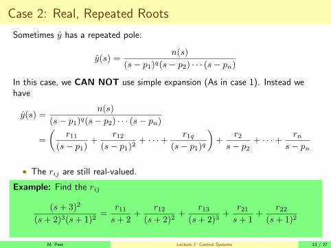
Case 2: Real, Repeated Roots
Sometimes y has a repeated pole:
y(s) =n(s)
(s− p1)q(s− p2) · · · (s− pn)
In this case, we CAN NOT use simple expansion (As in case 1). Instead wehave
y(s) =n(s)
(s− p1)q(s− p2) · · · (s− pn)
=
(r11
(s− p1)+
r12(s− p1)2
+ · · ·+ r1q(s− p1)q
)+
r2s− p2
+ · · ·+ rns− pn
• The rij are still real-valued.
Example: Find the rij
(s + 3)2
(s + 2)3(s + 1)2=
r11s + 2
+r12
(s + 2)2+
r13(s + 2)3
+r21s + 1
+r22
(s + 1)2
M. Peet Lecture 7: Control Systems 13 / 27

Case 2: Real, Repeated Roots
Problem: We have more coefficients to find.
• q coefficients for each repeated root.
First Step: Solve for r2, · · · , rn as before:If pi is not a repeated root, then
ri =n(pi)
(pi − p1)q · · · (pi − pi−1)(pi − pi+1) · · · (pi − pn)
M. Peet Lecture 7: Control Systems 14 / 27

Case 2: Real, Repeated Roots
New Step: Multiply by (s− p1)q to get the coefficient r1q.
y(s)(s− p1)q =
(r11
(s− p1)q
(s− p1)+ r12
(s− p1)q
(s− p1)2+ · · ·+ r1q
(s− p1)q
(s− p1)q
)+ r2
(s− p1)q
s− p2+ · · ·+ rn
(s− p1)q
s− pn
=(r11(s− p1)q−1 + r12(s− p1)q−2 + · · ·+ r1q
)+ r2
(s− p1)q
s− p2+ · · ·+ rn
(s− p1)q
s− pn
and evaluate at the point s = pi to get .
r1q = y(s)(s− p1)q|s=p1
• r1q is y(p1) with the repeated pole removed.
M. Peet Lecture 7: Control Systems 15 / 27

Case 2: Real, Repeated Roots
To find the remaining coefficients, we Differentiate:
y(s)(s− p1)q =(r11(s− p1)q−1 + r12(s− p1)q−2 + · · ·+ r1q
)+ r2
(s− p1)q
s− p2+ · · ·+ rn
(s− p1)q
s− pn
to get
d
ds(y(s)(s− p1)q)
=((q − 1)r11(s− p1)q−2 + (q − 2)r12(s− p1)q−3 + · · ·+ r1,(q−1)
)+
d
ds(s− p1)q
(r2
s− p2+ · · ·+ rn
s− pn
)Evaluating at the point s = p1.
d
ds(y(s)(s− p1)q) |s=p1
= r1,(q−1)
M. Peet Lecture 7: Control Systems 16 / 27

Case 2: Real, Repeated Roots
If we differentiate again, we get
d2
ds2(y(s)(s− p1)q)
=((q − 1)(q − 2)r11(s− p1)q−3 + · · ·+ 2r1,(q−2)
)+
d2
ds2(s− p1)q
(r2
s− p2+ · · ·+ rn
s− pn
)Evaluating at s− p1, we get
r1,(q−2) =1
2
d2
ds2(y(s)(s− p1)q) |s=p1
Extending this indefinitely
r1,j =1
(q − j − 1)!
dq−j−1
dsq−j−1(y(s)(s− p1)q) |s=p1
Of course, calculating this derivative is often difficult.
M. Peet Lecture 7: Control Systems 17 / 27
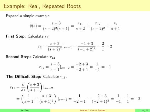
Example: Real, Repeated Roots
Expand a simple example
y(s) =s + 3
(s + 2)2(s + 1)=
r11s + 2
+r12
(s + 2)2+
r2s + 1
First Step: Calculate r2
r2 =s + 3
(s + 2)2|s=−1 =
−1 + 3
(−1 + 2)2=
2
1= 2
Second Step: Calculate r12
r12 =s + 3
s + 1|s=−2 =
−2 + 3
−2 + 1=
1
−1= −1
The Difficult Step: Calculate r11:
r11 =d
ds
(s + 3
s + 1
)|s=−2
=
(1
s + 1− s + 3
(s + 1)2
)|s=−2 =
1
−2 + 1− −2 + 3
(−2 + 1)2=
1
−1− 1
1= −2
M. Peet Lecture 7: Control Systems 18 / 27

Example: Real, Repeated Roots
So now we have
y(s) =s + 3
(s + 2)2(s + 1)=−2
s + 2+
−1
(s + 2)2+
2
s + 1
Question: what is the Inverse Fourier Transform of 1(s+2)2 ?
Recall the Power Exponential:
1
(s + a)m→ tm−1e−at
(m− 1)!
Finally, we have:
y(t) = −2e−2t − te−2t + 2e−t
0 1 2 3 4 5 6 7 8 9 100
0.05
0.1
0.15
0.2
0.25
0.3
0.35
t
y(t)
M. Peet Lecture 7: Control Systems 19 / 27

Case 3: Complex Roots
Most signals have complex roots (More common than repeated roots).
y(s) =3
s(s2 + 2s + 5)
has roots at s = 0, s = −1− 2ı, and s = −1 + 2ı.
Note that:
• Complex roots come in pairs.
• Simple partial fractions will work, but NOT RECOMMENDEDI Coefficients will be complex.I Solutions will be complex exponentials.I Require conversion to real functions.
Best to Separate out the Complex pairs as:
y(s) =n(s)
(s2 + as + b)(s− p1) · · · (s− pn)
M. Peet Lecture 7: Control Systems 20 / 27

Case 3: Complex Roots
Complex pairs have the expansion
n(s)
(s2 + as + b)(s− p1) · · · (s− pn)=
k1s + k2s2 + as + b
+r1
s− p1+ · · ·+ rn
s− pn
Note that there are two coefficients for each pair: k1 and k2.
NOTE: There are several different methods for finding k1 and k2.
First Step: Solve for r2, · · · , rn as normal.
Second Step: Clear the denominator. Multiply equation by all poles.
n(s) = (s2+as+b)(s−p1) · · · (s−pn)
(k1s + k2
s2 + as + b+
r1s− p1
+ · · ·+ rns− pn
)
Third Step: Solve for k1 and k2 by examining the coefficients of powers of s.
Warning: May get complicated or impossible for multiple complex pairs.
M. Peet Lecture 7: Control Systems 21 / 27

Case 3 Example
Take the example
y(s) =2(s + 2)
(s + 1)(s2 + 4)=
k1s + k2s2 + 4
+r1
s + 1
First Step: Find the simple coefficient r1.
r1 =2(s + 2)
s2 + 4|s=−1 = 2
−1 + 2
−12 + 4= 2
1
5=
2
5
Next Step: Multiply through by (s2 + 4)(s + 1).
2(s + 2) = (s + 1)(k1s + k2) + r1(s2 + 4)
Expanding and using r1 = 2/5 gives:
2s + 4 = (k1 + 2/5)s2 + (k2 + k1)s + k2 + 8/5
M. Peet Lecture 7: Control Systems 22 / 27

Case 3 Example
Recall the equation
2s + 4 = (k1 + 2/5)s2 + (k2 + k1)s + k2 + 8/5
Equating coefficients gives 3 equations:
• s2 term - 0 = k1 + 2/5
• s term - 2 = k2 + k1
• s0 term - 4 = k2 + 8/5
An over-determined system of equations (but consistent)
• First term gives k1 = −2/5
• Second term gives k2 = 2− k1 = 10/5 + 2/5 = 12/5
• Double-Check with last term: 4 = 12/5 + 8/5 = 20/5
M. Peet Lecture 7: Control Systems 23 / 27

Case 3 Example
So we have
y(s) =2(s + 2)
(s + 1)(s2 + 4)=
2
5
(1
s + 1− s− 6
s2 + 4
)=
2
5
(1
s + 1− s
s2 + 4+
6
s2 + 4
)y(t) =
2
5
(e−t − cos(2t) + 3 sin(2t)
)
0 5 10 15 20 25 30−1.5
−1
−0.5
0
0.5
1
1.5
t
y(t)
M. Peet Lecture 7: Control Systems 24 / 27
Case 3 Example
Now consider the solution to A Different Numerical Example: (Nise)
3
s(s2 + 2s + 5)=
3/5
s− 3
5
s + 2
s2 + 2s + 5
What to do with term:s + 2
s2 + 2s + 5?
We can rewrite as the combination of a frequency shift and a sinusoid:
s + 2
s2 + 2s + 5=
s + 2
s2 + 2s + 1 + 4=
(s + 1) + 1
(s + 1)2 + 4
=(s + 1)
(s + 1)2 + 4+
1
2
2
(s + 1)2 + 4
M. Peet Lecture 7: Control Systems 25 / 27
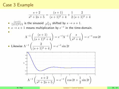
Case 3 Example
s + 2
s2 + 2s + 5=
(s + 1)
(s + 1)2 + 4+
1
2
2
(s + 1)2 + 4
• (s+1)(s+1)2+4 is the sinusoid s
s2+4 shifted by s→ s + 1.
• s→ s + 1 means multiplication by e−t in the time-domain.•
Λ−1(
(s + 1)
(s + 1)2 + 4
)= e−tΛ−1
(s
s2 + 4
)= e−t cos 2t
• Likewise Λ−1(
2
(s + 1)2 + 4
)= e−t sin 2t
0 1 2 3 4 5 6 7 8−0.4
−0.2
0
0.2
0.4
0.6
0.8
1
t
y(t)
Λ−1(
s + 2
s2 + 2s + 5
)= e−t
(cos 2t +
1
2sin 2t
)M. Peet Lecture 7: Control Systems 26 / 27

Summary
What have we learned today?
In this Lecture, you will learn: The Inverse Laplace Transform
• Simple Forms
The Partial Fraction Expansion
• How poles relate to dominant modes
• Expansion using single poles
• Repeated Poles
• Complex Pairs of PolesI Inverse Laplace
Next Lecture: Important Properties of the Response
M. Peet Lecture 7: Control Systems 27 / 27