Part A: Perturbation theory

W.R. Young 1

April 2017

1Scripps Institution of Oceanography, University of California at San Diego, La Jolla, CA 92093–0230,USA. wryoung@ucsd.edu

Contents

1 Introduction to perturbation theory 4

1.1 The goal of this class . . . . . . . . . . . . . . . . . . . . . . . . . . . . . . . . . . 41.2 Small parameters and really small parameters: ǫ versus ǫ2 . . . . . . . . . . . . . 51.3 An example: rectification of the ellipse . . . . . . . . . . . . . . . . . . . . . . . . 61.4 Some algebraic perturbation theory . . . . . . . . . . . . . . . . . . . . . . . . . . 81.5 Problems . . . . . . . . . . . . . . . . . . . . . . . . . . . . . . . . . . . . . . . . 13

2 Algebraic perturbation theory 15

2.1 Singular perturbation of polynomial equations . . . . . . . . . . . . . . . . . . . . 152.2 Iteration . . . . . . . . . . . . . . . . . . . . . . . . . . . . . . . . . . . . . . . . . 162.3 Double roots . . . . . . . . . . . . . . . . . . . . . . . . . . . . . . . . . . . . . . 182.4 An example with logarithms . . . . . . . . . . . . . . . . . . . . . . . . . . . . . . 192.5 Convergence . . . . . . . . . . . . . . . . . . . . . . . . . . . . . . . . . . . . . . . 212.6 Problems . . . . . . . . . . . . . . . . . . . . . . . . . . . . . . . . . . . . . . . . 22

3 Autonomous differential equations 25

3.1 The phase line . . . . . . . . . . . . . . . . . . . . . . . . . . . . . . . . . . . . . 253.2 Population growth — the logistic equation . . . . . . . . . . . . . . . . . . . . . . 263.3 The phase plane . . . . . . . . . . . . . . . . . . . . . . . . . . . . . . . . . . . . 273.4 Matlab ODE tools . . . . . . . . . . . . . . . . . . . . . . . . . . . . . . . . . . . 303.5 The linear oscillator . . . . . . . . . . . . . . . . . . . . . . . . . . . . . . . . . . 323.6 Nonlinear oscillators . . . . . . . . . . . . . . . . . . . . . . . . . . . . . . . . . . 333.7 Problems . . . . . . . . . . . . . . . . . . . . . . . . . . . . . . . . . . . . . . . . 37

4 Regular perturbation of ordinary differential equations 42

4.1 Initial value problems: the projectile problem . . . . . . . . . . . . . . . . . . . . 424.2 Boundary value problems: belligerent drunks . . . . . . . . . . . . . . . . . . . . 454.3 Failure of RPS: singular perturbation problems . . . . . . . . . . . . . . . . . . . 484.4 Problems . . . . . . . . . . . . . . . . . . . . . . . . . . . . . . . . . . . . . . . . 52

5 Regular perturbation of partial differential equations 55

5.1 Thermal diffusion in solids . . . . . . . . . . . . . . . . . . . . . . . . . . . . . . . 555.2 Steady heat diffusion through a corrugated slab . . . . . . . . . . . . . . . . . . . 555.3 Slow variations . . . . . . . . . . . . . . . . . . . . . . . . . . . . . . . . . . . . . 585.4 A slowly rotating self-gravitating mass . . . . . . . . . . . . . . . . . . . . . . . 595.5 Problems . . . . . . . . . . . . . . . . . . . . . . . . . . . . . . . . . . . . . . . . 63

1

6 Boundary Layers 65

6.1 Stommel’s dirt pile . . . . . . . . . . . . . . . . . . . . . . . . . . . . . . . . . . . 656.2 Leading-order solution of the dirt-pile model . . . . . . . . . . . . . . . . . . . . . 676.3 Stommel’s problem at infinite order . . . . . . . . . . . . . . . . . . . . . . . . . . 696.4 A nonlinear Stommel problem . . . . . . . . . . . . . . . . . . . . . . . . . . . . . 726.5 Problems . . . . . . . . . . . . . . . . . . . . . . . . . . . . . . . . . . . . . . . . 75

7 More boundary layer theory 77

7.1 Variable speed . . . . . . . . . . . . . . . . . . . . . . . . . . . . . . . . . . . . . 777.2 A second-order BVP with a boundary layer . . . . . . . . . . . . . . . . . . . . . 837.3 Other BL examples . . . . . . . . . . . . . . . . . . . . . . . . . . . . . . . . . . . 847.4 Problems . . . . . . . . . . . . . . . . . . . . . . . . . . . . . . . . . . . . . . . . 87

8 Multiple scale theory 89

8.1 Introduction to two-timing . . . . . . . . . . . . . . . . . . . . . . . . . . . . . . . 898.2 The Duffing oscillator . . . . . . . . . . . . . . . . . . . . . . . . . . . . . . . . . 918.3 The quadratic oscillator . . . . . . . . . . . . . . . . . . . . . . . . . . . . . . . . 938.4 Symmetry and universality of the Landau equation . . . . . . . . . . . . . . . . . 958.5 Parametric instability . . . . . . . . . . . . . . . . . . . . . . . . . . . . . . . . . 968.6 The resonantly forced Duffing oscillator . . . . . . . . . . . . . . . . . . . . . . . 978.7 Problems . . . . . . . . . . . . . . . . . . . . . . . . . . . . . . . . . . . . . . . . 101

9 Rapid fluctuations, Stokes drift and averaging 103

9.1 A Lotka-Volterra Example . . . . . . . . . . . . . . . . . . . . . . . . . . . . . . . 1039.2 The averaging theorem . . . . . . . . . . . . . . . . . . . . . . . . . . . . . . . . . 1059.3 Stokes drift . . . . . . . . . . . . . . . . . . . . . . . . . . . . . . . . . . . . . . . 1069.4 The Kapitsa pendulum . . . . . . . . . . . . . . . . . . . . . . . . . . . . . . . . . 1089.5 Problems . . . . . . . . . . . . . . . . . . . . . . . . . . . . . . . . . . . . . . . . 109

10 Eigenvalue problems 113

10.1 Regular Sturm-Liouville problems . . . . . . . . . . . . . . . . . . . . . . . . . . . 11310.2 Properties of Sturm-Liouville eigenproblems . . . . . . . . . . . . . . . . . . . . . 11410.3 Trouble with BVPs . . . . . . . . . . . . . . . . . . . . . . . . . . . . . . . . . . . 11610.4 The eigenfunction expansion method . . . . . . . . . . . . . . . . . . . . . . . . . 11810.5 Eigenvalue perturbations . . . . . . . . . . . . . . . . . . . . . . . . . . . . . . . . 12010.6 The vibrating string . . . . . . . . . . . . . . . . . . . . . . . . . . . . . . . . . . 12110.7 Problems . . . . . . . . . . . . . . . . . . . . . . . . . . . . . . . . . . . . . . . . 123

11 WKB 127

11.1 The WKB approximation . . . . . . . . . . . . . . . . . . . . . . . . . . . . . . . 12711.2 Some examples . . . . . . . . . . . . . . . . . . . . . . . . . . . . . . . . . . . . . 12911.3 Validity of WKB and higher order terms . . . . . . . . . . . . . . . . . . . . . . 13311.4 Eigenproblems . . . . . . . . . . . . . . . . . . . . . . . . . . . . . . . . . . . . . 13411.5 Using bvp4c . . . . . . . . . . . . . . . . . . . . . . . . . . . . . . . . . . . . . . . 13911.6 Problems . . . . . . . . . . . . . . . . . . . . . . . . . . . . . . . . . . . . . . . . 142

12 Internal boundary layers 148

12.1 A linear example . . . . . . . . . . . . . . . . . . . . . . . . . . . . . . . . . . . . 148

2

13 Initial layers 152

13.1 The over-damped oscillator . . . . . . . . . . . . . . . . . . . . . . . . . . . . . . 15213.2 Problems . . . . . . . . . . . . . . . . . . . . . . . . . . . . . . . . . . . . . . . . 153

14 Boundary layers in fourth-order problems 155

14.1 A fourth-order differential equation . . . . . . . . . . . . . . . . . . . . . . . . . . 15514.2 Problems . . . . . . . . . . . . . . . . . . . . . . . . . . . . . . . . . . . . . . . . 157

3

Lecture 1

Introduction to perturbation theory

1.1 The goal of this class

The goal is to teach you how to obtain approximate analytic solutions to applied-mathematicalproblems that can’t be solved “exactly”.

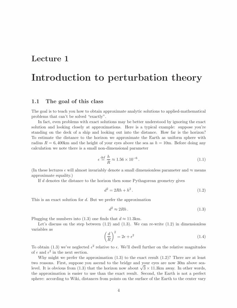
In fact, even problems with exact solutions may be better understood by ignoring the exactsolution and looking closely at approximations. Here is a typical example: suppose you’restanding on the deck of a ship and looking out into the distance. How far is the horizon?To estimate the distance to the horizon we approximate the Earth as uniform sphere withradius R = 6, 400km and the height of your eyes above the sea as h = 10m. Before doing anycalculation we note there is a small non-dimensional parameter

ǫdef=

h

R≈ 1.56× 10−6 . (1.1)

(In these lectures ǫ will almost invariably denote a small dimensionless parameter and ≈ meansapproximate equality.)

If d denotes the distance to the horizon then some Pythagorean geometry gives

d2 = 2Rh+ h2 . (1.2)

This is an exact solution for d. But we prefer the approximation

d2 ≈ 2Rh . (1.3)

Plugging the numbers into (1.3) one finds that d ≈ 11.3km.Let’s discuss on the step between (1.2) and (1.3). We can re-write (1.2) in dimensionless

variables as (d

R

)2

= 2ǫ+ ǫ2 (1.4)

To obtain (1.3) we’ve neglected ǫ2 relative to ǫ. We’ll dwell further on the relative magnitudesof ǫ and ǫ2 in the next section.

Why might we prefer the approximation (1.3) to the exact result (1.2)? There are at leasttwo reasons. First, suppose you ascend to the bridge and your eyes are now 30m above sea-level. It is obvious from (1.3) that the horizon now about

√3 × 11.3km away. In other words,

the approximation is easier to use than the exact result. Second, the Earth is not a perfectsphere: according to Wiki, distances from points on the surface of the Earth to the center vary

4

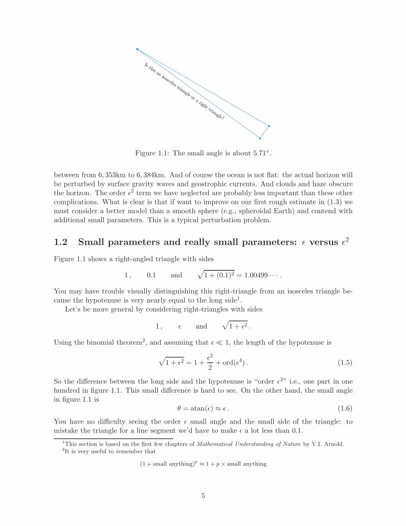
Is this anisosceles triangle or a right triangle?

Figure 1.1: The small angle is about 5.71.

between from 6, 353km to 6, 384km. And of course the ocean is not flat: the actual horizon willbe perturbed by surface gravity waves and geostrophic currents. And clouds and haze obscurethe horizon. The order ǫ2 term we have neglected are probably less important than these othercomplications. What is clear is that if want to improve on our first rough estimate in (1.3) wemust consider a better model than a smooth sphere (e.g., spheroidal Earth) and contend withadditional small parameters. This is a typical perturbation problem.

1.2 Small parameters and really small parameters: ǫ versus ǫ2

Figure 1.1 shows a right-angled triangle with sides

1 , 0.1 and√

1 + (0.1)2 = 1.00499 · · · .

You may have trouble visually distinguishing this right-triangle from an isosceles triangle be-cause the hypotenuse is very nearly equal to the long side1.

Let’s be more general by considering right-triangles with sides

1 , ǫ and√

1 + ǫ2 .

Using the binomial theorem2, and assuming that ǫ≪ 1, the length of the hypotenuse is

√

1 + ǫ2 = 1 +ǫ2

2+ ord(ǫ4) . (1.5)

So the difference between the long side and the hypotenuse is “order ǫ2” i.e., one part in onehundred in figure 1.1. This small difference is hard to see. On the other hand, the small anglein figure 1.1 is

θ = atan(ǫ) ≈ ǫ . (1.6)

You have no difficulty seeing the order ǫ small angle and the small side of the triangle: tomistake the triangle for a line segment we’d have to make ǫ a lot less than 0.1.

1This section is based on the first few chapters of Mathematical Understanding of Nature by V.I. Arnold.2It is very useful to remember that

(1 + small anything)p ≈ 1 + p× small anything

5

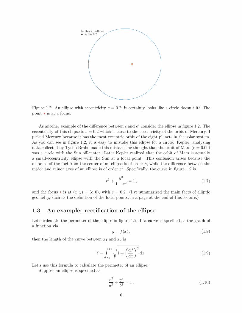
Is this an ellipseor a circle?

Figure 1.2: An ellipse with eccentricity e = 0.2; it certainly looks like a circle doesn’t it? Thepoint ∗ is at a focus.

As another example of the difference between ǫ and ǫ2 consider the ellipse in figure 1.2. Theeccentricity of this ellipse is e = 0.2 which is close to the eccentricity of the orbit of Mercury. Ipicked Mercury because it has the most eccentric orbit of the eight planets in the solar system.As you can see in figure 1.2, it is easy to mistake this ellipse for a circle. Kepler, analyzingdata collected by Tycho Brahe made this mistake: he thought that the orbit of Mars (e = 0.09)was a circle with the Sun off-center. Later Kepler realized that the orbit of Mars is actuallya small-eccentricity ellipse with the Sun at a focal point. This confusion arises because thedistance of the foci from the center of an ellipse is of order e, while the difference between themajor and minor axes of an ellipse is of order e2. Specifically, the curve in figure 1.2 is

x2 +y2

1− e2= 1 , (1.7)

and the focus ∗ is at (x, y) = (e, 0), with e = 0.2. (I’ve summarized the main facts of ellipticgeometry, such as the definition of the focal points, in a page at the end of this lecture.)

1.3 An example: rectification of the ellipse

Let’s calculate the perimeter of the ellipse in figure 1.2. If a curve is specified as the graph ofa function via

y = f(x) , (1.8)

then the length of the curve between x1 and x2 is

ℓ =

∫ x2

x1

√

1 +

(df

dx

)2

dx. (1.9)

Let’s use this formula to calculate the perimeter of an ellipse.Suppose an ellipse is specified as

x2

a2+y2

b2= 1 . (1.10)

6

0 0.1 0.2 0.3 0.4 0.5 0.6 0.7 0.8 0.9 1e

0.6

0.65

0.7

0.75

0.8

0.85

0.9

0.95

1

reductionfactorf

Figure 1.3: The “reduction factor” f(e) in (1.17) is the solid black curve. The two-termapproximation in (1.19) is the blue dashed curve. The three and four term approximations (thedash-dot and dotted curves) from (1.21) lie even closer to the black curve.

For the portion of the ellipse above the x-axis (i.e., y > 0) we have

y = b

√

1− x2

a2︸ ︷︷ ︸

f(x)

, anddf

dx= − b

a2x

√

1− x2

a2

. (1.11)

Using symmetry, and results from the appendix “elliptic anatomy”,

b =√

1− e2 a . (1.12)

Thus the perimeter is

ℓ = 4

∫ a

0

√

a2 − e2x2

a2 − x2dx , (1.13)

= 4a

∫ 1

0

√

1− e2v2

1− v2dv . (1.14)

Above we’ve used the change of variable x = av to tidy the integral so that it becomes non-dimensional and contains only the eccentricity e. We can try to evaluate the integral analyticallyby making a further substitution

v = sin θ , and thereforedv√1− v2

= dθ . (1.15)

The integral becomes

ℓ = 4a

∫ π/2

0

√

1− e2 sin2 θ dθ . (1.16)

As a sanity check, notice that if e = 0 the perimeter in (1.16) is 2πa.Students of applied mathematics used to learn to recognize elliptic integrals and many other

special functions. These days students probably use mathematica to discover that the integral

7

in (1.16) is a complete elliptic integral of the second kind. Here is answer written in DLMF

notation

ℓ = 2πa × 2

πE(e)

︸ ︷︷ ︸

f

, (1.17)

where f is the “reduction factor” relative to a circle with radius a. It is difficult to deny thatthis exact answer is useful because both mathematica and matlab have these elliptic integralshardwired3. However, if we are interested in quickly knowing the perimeter of the near-circlein figure 1.2 then we can approximately evaluate (1.16) like this4

ℓ ≈ 4a

∫ π/2

0

(1− 1

2e2 sin2 θ

)dθ , (1.18)

= 2πa(1− 1

4e2)

︸ ︷︷ ︸

≈f

. (1.19)

Figure 1.3 compares the approximation f ≈ 1 − e2/4 to the elliptic-function answer. Withe = 0.2 the simple approximation is probably good enough for most purposes. Of course, to usean approximation with some confidence we must have some estimate of the size of the error.

Exercise: explain why f(1) = 2/π = 0.6366 · · ·

Applied mathematics is concerned with making precise approximations in which the erroris both understood and controllable. We should also strive to make the error smaller by somesystematic method. Here we can do this by using more terms in the binomial expansion of√

1− e2 sin2 θ. Let’s use four terms and indicate the form of the first neglected term:

√

1− e2 sin2 θ = 1− 12e

2 sin2 θ − 18e

4 sin4 θ − 116e

6 sin6 θ + ord(e8). (1.20)

Integrating over θ, our new improved approximation to the reduction factor f is

f = 1− 14e

2 − 364e

4 − 5256e

6 + ord(e8). (1.21)

In figure 1.3 there is a systematic improvement as we use more terms in the series.

1.4 Some algebraic perturbation theory

The quadratic equationx2 − πx+ 2 = 0 , (1.22)

has the exact solutions

x = π2 ±

√

π2

4 − 2 = 2.254464 and 0.887129 . (1.23)

3However mathematica and matlab use a different convention from the DLMF in defining the completeelliptic integrals. Using the convention in mathematica and matlab f = 2E(e2)/π. I discovered this bug whenthe approximation in (1.19) did not agree with the “exact answer”.

4Notice

π

2=

∫ π/2

0

cos2 θ + sin2 θ dθ , and by quarter-wavelength symmetry

∫ π/2

0

cos2 θ dθ =

∫ π/2

0

sin2 θ dθ .

8

To introduce the main idea of perturbation theory, let’s pretend that calculating a square rootis a big deal. We notice that if we replace π by 3 in (1.22) then the resulting quadratic equationnicely factors and the roots are just x = 1 and x = 2. Because π is close to 3, our hope is thatthe roots of (1.22) are close to 1 and 2. Perturbation theory makes this intuition precise andsystematically improves our initial approximations x ≈ 1 and x ≈ 2.

A regular perturbation series

We use perturbation theory by writing

π = 3 + ǫ , (1.24)

and assuming that the solutions of

x2 − (3 + ǫ)x+ 2 = 0 , (1.25)

are given by a regular perturbation series (RPS):

x = x0 + ǫx1 + ǫ2x2 + · · · (1.26)

We are assuming that the xn’s above do not depend on ǫ. Putting (1.26) into (1.25) we have

x20 + ǫ 2x0x1+ǫ2 (2x0x2 + x21) + ǫ3 (2x0x3 + 2x1x2) (1.27)

− (3 + ǫ)(x0 + ǫx1 + ǫ2x2 + ǫ3x3) + 2 = ord(ǫ4). (1.28)

The notation “ord(ǫ4)” means that we are suppressing some unnecessary information, but weare indicating that the largest unwritten terms are all proportional to ǫ4. We’re assuming thatthe expansion (1.26) is unique so we can match up powers of ǫ in (1.28) and obtain a hierarchyof equations for the unknown coefficients xn in (1.26).

The leading-order terms from (1.28) are

ǫ0 : x20 − 3x0 + 2 = 0 , ⇒ x0 = 1 or 2 . (1.29)

Quadratic equations have two roots and the important point is that indeed the leading orderapproximation above delivers two roots: this is a regular perturbation problem. We’ll soonsee examples in which the leading approximation provides only one root: these problems aresingular perturbation problems.

Let’s take x0 = 1. The next three orders are then

ǫ1 : (2x0 − 3)x1 − x0 = 0 , ⇒ x1 =x0

2x0 − 3= −1 , (1.30)

ǫ2 : (2x0 − 3)x2 + x21 − x1 = 0 , ⇒ x2 =x1 − x212x0 − 3

= 2 , (1.31)

ǫ3 : (2x0 − 3)x3 + 2x1x2 − x2 = 0 , ⇒ x3 =x2(1− 2x1)

2x0 − 3= −6 , (1.32)

The resulting perturbation expansion is

x = 1− ǫ+ 2ǫ2 − 6ǫ3 + ord(ǫ4) . (1.33)

With ǫ = π − 3 we find x = 0.881472 + ord(ǫ4).

9

Exercise: Determine a few terms in the RPS of the root x0 = 2.

This example illustrates the main features of perturbation theory. When faced with adifficult problem one should:

1. Find an easy problem that’s close to the difficult problem. It helps if the easier problemhas a simple analytic solution.

2. Quantify the difference between the two problems by introducing a small parameter ǫ.

3. Assume that the answer is in the form of a perturbation expansion, such as (1.26).

4. Compute terms in the perturbation expansion.

5. Solve the difficult problem by summing the series with the appropriate value of ǫ.

Step 4 above also deserves some discussion. In this step we are sequentially solving ahierarchy of linear equations:

(2x0 − 3)xn+1 = R(x0, x1, · · · xn) . (1.34)

We can determine xn+1 because we can divide by (2x0−3): fortunately x0 6= 3/2. This structureoccurs in other simple perturbation problems: we confront the same linear problem at everylevel of the hierarchy and we have to solve this problem5 repeatedly.

Example: As a non-polynomial example consider

x2 − 1 = ǫex . (1.35)

Setting ǫ = 0 we see there are roots at x = −1 and x = +1. Let’s use a regular perturbation series (RPS)

x = 1︸︷︷︸

x0

+ǫx1 + ǫ2x2 + · · · (1.36)

to see how the root at x = 1 varies with ǫ. We’re going to calculate x1 and x2.

To substitute the series (1.36) into (1.35) we first need

e1+ǫx1+ǫ2x2 = e1 eǫx1+ǫ2x2+ord(ǫ3) , (1.37)

= e[

1 +(ǫx1 + ǫ2x2

)+ 1

2

(ǫx1 + ǫ2x2

)2+ ord

(ǫ3)]

, (1.38)

= e[1 + ǫx1 + ǫ2

(x2 +

12x21

)+ ord

(ǫ3)]. (1.39)

Notice how we have systematically simplified the expressions above by dropping all ǫ3 terms. Substitutingthe RPS into the transcendental equation (1.35), we discover that we have worked too hard in (1.39): ifwe require only x1 and x2 then we could have consigned terms of order ǫ2 in (1.39) to the dust–bin. Wedetermine x1 and x2 from

2ǫx1 + ǫ2(2x2 + x2

1

)= ǫe + ǫ2ex1 + ord

(ǫ3). (1.40)

Matching powers of ǫ we find x1 = e/2 and x2 = e2/8.

5Mathematicians would say that we are inverting the linear operator — this language seems pretentious inthis simple example. But we’ll soon see examples in which it is appropriate.

10

A singular perturbation

Now consider another quadratic equation

ǫx2 + x− 1 = 0 , (1.41)

again with ǫ ≪ 1. Let’s proceed using the method that worked in the previous example: pickthe low-hanging fruit by setting ǫ = 0 and solving the simplified equation. This gives x ≈ 1.We’re alarmed because already the problem seems very different from the previous example:although the full problem has two solutions, the ǫ = 0 equation has only one root. We’ll returnto this example in the next lecture and figure out what happened to the missing root.

Let’s proceed to understand how the root near x = 1 changes with ǫ. Again we use an RPS:

x = 1︸︷︷︸

x0

+ǫx1 + ǫ2x2 + · · · (1.42)

Substituting into the quadratic equation (1.41) we have

ǫ(1 + 2ǫx1 + ǫ22x2 + ǫ2x21

)+ ǫx1 + ǫ2x2 + ǫ3x3 + ord

(ǫ4)= 0 . (1.43)

Now match up powers of ǫ:

ǫ1 : 1 + x1 = 0 , ⇒ x1 = −1 , (1.44)

ǫ2 : 2x1 + x2 = 0 , ⇒ x2 = 2 , (1.45)

ǫ3 : 2x2 + x21 + x3 = 0 , ⇒ x3 = −5 . (1.46)

To summarizex = 1− ǫ+ 2ǫ2 − 5ǫ3 + ord

(ǫ4). (1.47)

This calculation is conceptually identical to our earlier example in (1.29) through (1.33). Butthe procedure is never going to help us find the missing root.

The quadratic (1.41) is a simple example of a singular perturbation problem: the problemwith non-zero ǫ has two roots, while the ǫ = 0 problem has only one. Thus the ǫ 6= 0 problem isfundamentally different from the ǫ = 0 problem. Of course one can solve the quadratic equation(1.41) exactly and figure out what’s happening to both roots as ǫ → 0. I suggest you do thatbefore next lecture.

11

Appendix: Summary of elliptic anatomy

An ellipse is a plane curve enclosing two focal points such that the sum of the distancesto the two foci is constant for every point on the ellipse. In figure (1.4) the foci are on thex-axis at x = ±ea and ellipse is defined by

√

(x− ea)2 + y2︸ ︷︷ ︸

def= r+

+√

(x+ ea)2 + y2︸ ︷︷ ︸

def= r−

= 2a . (1)

If e = 0 then the ellipse becomes a circle with radius a. With some algebra you can showthat (1) is equivalent to

x2

a2+y2

b2= 1 , (2)

whereb =

√

1− e2 a .

The lengths a and b are the semi-major and semi-minor axes respectively. If e ≪ 1 thenthe difference between a and b is order e2.

+ea−ea +a−a

b

−b

r−

r+

Figure 1.4: An ellipse with e = 0.75.

If the ellipse is a mirror and there is a light source at one of the foci then the light raysreflecting specularly from the mirror all pass through the other focal point.

12

1.5 Problems

Problem 1.1. Because 10 is close to 9 we suspect that√10 is close to

√9 = 3. (i) Define x(ǫ)

byx(ǫ)2 = 9 + ǫ , (1.48)

and assume that x(ǫ) has an RPS like (1.26). Calculate the first four terms, x0 through x3. (ii)Take ǫ = 1 and compare your estimate of

√10 with a six decimal place computation. (iii) Now

solve (1.48) with the binomial expansion and verify that the resulting series is the same as theRPS from part (ii). What is the radius of convergence of the series?

Problem 1.2. Find a two-term approximation to all five roots of

x5 − x+ ǫ = 0 . (1.49)

Take ǫ = 1/4 and compare your approximation to a numerical solution.

Problem 1.3. Consider the transcendental equation

x2 − 1 = ǫex2. (1.50)

If ǫ = 0 there is a root x = 1. Find the first three terms in the ǫ → 0 regular perturbationexpansion of this root.

Problem 1.4. Assume the Earth is a perfect sphere with radius R = 6, 400km and it wrappedaround the equator by a rope with length 6, 400km plus one meter. (i) Suppose the rope ispulled to a uniform height h above the surface of the Earth — calculate h? (This is an easywarm-up.) (ii) Suppose the rope is grabbed at a point and that point is hoisted vertically to aheight H till the rope is taut. Estimate H.

Problem 1.5. Consider

A(n) =

∫∞

0

dt

1 + t2 + tn(1.51)

Plot the integrand on the interval 0 < t < 2 for n = 50 and 100. After studying this plot, devisean n≫ 1 approximation to A(n) and test your approximation by comparison with a numericalevaluation of A(100).

Problem 1.6. Consider

B(n) =

∫∞

0

dt

(1 + t2)(1 + tn)(1.52)

Plot the integrand on the interval 0 < t < 2 for n = 50 and 100. After studying this plot, devisean n≫ 1 approximation to B(n) and test your approximation by comparison with a numericalevaluation of F (100). You’ll know you’ve done this problem correctly if careful comparison ofthe numerics with your approximation is very surprising.

13

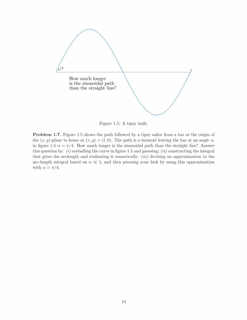
How much longeris the sinusoidal paththan the straight line?

π/4 ℓ

Figure 1.5: A tipsy walk.

Problem 1.7. Figure 1.5 shows the path followed by a tipsy sailor from a bar at the origin ofthe (x, y)-plane to home at (x, y) = (ℓ, 0). The path is a sinusoid leaving the bar at an angle α;in figure 1.5 α = π/4. How much longer is the sinusoidal path than the straight line? Answerthis question by: (i) eyeballing the curve in figure 1.5 and guessing; (ii) constructing the integralthat gives the arclength and evaluating it numerically; (iii) devising an approximation to thearc-length integral based on α ≪ 1, and then pressing your luck by using this approximationwith α = π/4.

14

Lecture 2

Algebraic perturbation theory

2.1 Singular perturbation of polynomial equations

Let’s start with the example from last lecture

ǫx2 + x− 1 = 0 . (2.1)

Setting ǫ = 0, we found x = 1 and we then proceeded to nail down this root with the regularperturbation series (RPS) in (1.47). But a quadratic equation has two roots: we’re missing aroot. Peeking at the answer, we find

x =−1±

√1 + 4ǫ

2ǫ, (2.2)

or

x =

1− ǫ+ 2ǫ2 − 5ǫ3 + · · ·−ǫ−1 − 1 + ǫ− 2ǫ2 + 5ǫ3 + · · ·

(2.3)

The missing root is going to infinity as ǫ→ 0. Notice that the term we blithely dropped, namelyǫx2, is therefore ord(ǫ−1). Dropping a big term is a mistake.

We could have discovered the missing root by looking for two-term dominant balances in(2.1):

ǫx2 + x︸ ︷︷ ︸

dominant balance

−1 = 0 . (2.4)

The balance above implies that x = −ǫ−1. The balance is consistent because the neglectedterm in (2.4) (the −1) is smaller than the two retained terms as ǫ → 0. Once we know that xis varying as ǫ−1 we can rescale by defining

Xdef= ǫx . (2.5)

The variable X remains finite as ǫ→ 0, and substituting (2.5) into (2.1) we find that X satisfiesthe rescaled equation

X2 +X − ǫ = 0 . (2.6)

Now we can find the big root via an RPS

X = X0 + ǫX1 + ǫ2X2 + · · · (2.7)

This procedure reproduces the expansion that begins with −ǫ−1 in (2.3).

15

Notice that (2.5) is “only” a change in notation, and (2.6) is equivalent to (2.1). Butnotation matters: in terms of x the problem is singular while in terms of X the problem isregular.

Example: Find ǫ≪ 1 expansions of the roots of

ǫx3 + x− 1 = 0 . (2.8)

One root is obviously obtained via an RPS

x = 1− ǫ+ ord(ǫ2) . (2.9)

But there are two missing roots. A dominant balance between the first two terms in (2.9),

ǫx3 + x ≈ 0 , (2.10)

implies that x varies as ǫ−1/2. This balance is consistent, so rescale

Xdef= ǫ1/2x . (2.11)

This definition ensures that X is order unity as ǫ→ 0. The rescaled equation is

X3 +X −√ǫ = 0 , (2.12)

and there is now a regular perturbation problem with small parameter√ǫ:

X = X0 +√ǫX1 +

(√ǫ)2X2 + · · · (2.13)

The leading order terms are

X30 +X0 = 0 ⇒ X0 = ±i and X0 = 0 . (2.14)

The solution X0 = 0 is reproducing the solution back in (2.9). Let’s focus on the other two roots, X0 = ±i.At next order the problem is

√ǫ : 3X2

0X1 +X1 − 1 = 0 , ⇒ X1 =1

3X20 + 1

= −1

2. (2.15)

For good value

(√ǫ)2

: 3X20X2 +X2 + 3X0X

21 = 0 , ⇒ X2 = − 3X0X

21

3X20 + 1

= ±3

8i . (2.16)

We write the expansion in terms of our original variable as

x = ± i√ǫ− 1

2±

√ǫ3 i

8+ ord

(ǫ1). (2.17)

Example: Find leading-order expressions for all six roots of

ǫ2x6 − ǫx4 − x3 + 8 = 0 , as ǫ→ 0. (2.18)

This is from BO section 7.2.

2.2 Iteration

Now let’s consider the method of iteration — this is an alternative to the RPS. Iteration requiresa bit of initial ingenuity. But in cases where the form of the expansion is not obvious, iterationis essential. (One of the strengths of H is that it emphasizes the utility of iteration.)

16

Solution of a quadratic equation by iteration

We can rewrite the quadratic equation (1.25) as

(x− 1)(x− 2) = ǫx . (2.19)

If we interested in the effect of ǫ on the root x = 1 then we rearrange this further as

x = 1 + ǫx

x− 2︸ ︷︷ ︸

def= f(x)

. (2.20)

We iterate by first dropping the ǫ-term on the right — this provides the first guess x(0) = 1.At the next iteration we keep the ǫ-term with f evaluated at x(0):

x(1) = 1 + ǫf(

x(0))

= 1− ǫ . (2.21)

We continue to improve the approximation with more and more iterates:

x(n+1) = 1 + f(

x(n))

. (2.22)

So the second iteration is

x(2) = 1 + ǫf(

x(1))

= 1− ǫ1− ǫ

1 + ǫ. (2.23)

This is not an RPS — if we want an answer ordered in powers of ǫ then we must simplify (2.23)further as

x(2) = 1− ǫ (1− ǫ)(1− ǫ+ ord(ǫ2)

)= 1− ǫ+ 2ǫ2 + ord(ǫ3) . (2.24)

I suspect there is no point in keeping the ǫ3 in (2.24) because it is probably not correct — I amguessing that we have to iterate one more time to get the correct ǫ3 term.

Exercise: use iteration to locate the root near x = 2.

Another example of iteration

Considering the equation4− x2 = ǫ lnx , (2.25)

with 0 < ǫ ≪ 1, we see (draw a graph) that there is a positive real solution close to x = 2. Toimprove on x ≈ 2 we rewrite the equation as

x = 2− ǫ lnx

2 + x. (2.26)

If we drop the ǫ-term we get a first approximation x(1) = 2, and the next iterate is

x(2) = 2− ǫ ln 2

4, (2.27)

and again

x(3) = 2− ǫ ln(2− ǫ ln 2

4

)

4− ǫ ln 24

. (2.28)

17

We can develop an RPS by simplifying x(3) as

x(3) = 2− ǫ

4

(

1 + ǫln 2

16

)[

ln 2 + ln(1− ǫ

ln 2

8

)

︸ ︷︷ ︸

=−ǫ ln 28

+ord(ǫ2)

]

+ ord(ǫ3) , (2.29)

= 2− ln 2

4ǫ+

ln 2

64(2− ln 2) ǫ2 + ord(ǫ3) . (2.30)

2.3 Double roots

Now considerx2 − 2x+ 1︸ ︷︷ ︸

(x−1)2

−ǫf(x) = 0 . (2.31)

where f(x) is some function of x. Section 1.3 of H discusses the case f(x) = x2 — with asurfeit of testosterone we attack the general case.

We try the RPS:x = x0 + ǫx1 + ǫ2x2 + · · · (2.32)

We must expand f(x) with a Taylor series:

f(x0 + ǫx1 + ǫ2x2 + · · ·

)= f(x0) + ǫx1f

′(x0) + ǫ2(

x2f′(x0) +

1

2x21f

′′(x0)

)

+ ord(ǫ3).

(2.33)

This is not as bad as it looks — we’ll only need the first term, f(x0), though that may not beobvious at the outset.

The leading term in (2.31) is

x20 − 2x0 + 1 = 0 , ⇒ x0 = 1 , (twice). (2.34)

There is a double root. At next order there is a problem:

ǫ1 : 2x1 − 2x1︸ ︷︷ ︸

=0

−f(1) = 0 . (2.35)

Unless f(1) happens to vanish, we’re stuck. The problem is that we assumed that the solutionhas the form in (2.32), and it turns out that this assumption is wrong. The perturbation methodkindly tells us this by producing the contradiction in (2.35).

To find the correct form of the expansion we use iteration: rewrite (2.31) as

x = 1±√

ǫf(x) . (2.36)

and starting with x(0) = 1, iterate with

x(n+1) = 1±√

ǫf(x(n−1)

). (2.37)

At the first iteration we findx(1) = 1±

√

ǫf (1) . (2.38)

There is a√ǫ which was not anticipated by the RPS back in (2.32).

18

Exercise: Go through another iteration cycle to find x(2).

Iteration has shown us the way forward: we proceed assuming that the correct RPS isprobably

x = x0 + ǫ1/2x1 + ǫx2 + ǫ3/2x3 + · · · (2.39)

At leading order we find x0 = 1, and at next order

ǫ1/2 : 2x1 − 2x1 = 0 . (2.40)

This is surprising, but it is not a contradiction: x1 is not determined at this order. We have toendure some suspense — we go to next order and find

ǫ1 : 2(x0 − 1)x2︸ ︷︷ ︸

=0

+x21 − f(x0) = 0 , ⇒ x1 = ±√

f(1) . (2.41)

The RPS has now managed to reproduce the first iterate x(1). Going to order ǫ3/2, we find thatx3 is undetermined and

x2 =12f

′(1) . (2.42)

The solution we constructed is

x = 1±√

ǫf(1) +ǫ

2f ′(1) + ord

(

ǫ3/2)

. (2.43)

This example teaches us that a perturbation “splits” double roots. The splitting is ratherlarge: adding the order ǫ perturbation in (2.31) moves the roots apart by order

√ǫ ≫ ǫ.

This sensitivity to small perturbations is obvious geometrically — draw a parabola P touchingthe x-axis at some point, and move P downwards by small distance. The small movementproduces two roots separated by a distance that is clearly much greater than the small verticaldisplacement of P . If P moves upwards (corresponding to f(1) < 0 in the example above) thenthe roots split off along the imaginary axis.

2.4 An example with logarithms

I’ll discuss the example1 from H section 1.4:

xe−x = ǫ . (2.44)

It is easy to see that if 0 < ǫ ≪ 1 there is a small solution and a big solution. It is straightforwardto find the small solution in terms of ǫ. Here we discuss the more difficult problem of findingthe big solution.

Exercise: Show that the small solution is x(ǫ) = ǫ+ ǫ2 + 32ǫ3 + ord(ǫ4).

To get a handle on (2.44), we take the logarithm and write the result as

x = L1 + lnx , (2.45)

where

L1def= ln

1

ǫ. (2.46)

19

0 1 2 3 4 5 6 7 8 9 1010

−3

10−2

10−1

100

x

ǫ

exactL

1

L1+L

2

L1+L

2+L

1/L

2

L1+L

2+L

2/L

1+ P(L

2)/L

12

Figure 2.1: Comparison of ǫ = xe−x with increasingly accurate small-ǫ approximations to theinverse function ǫ(x).

Note if 0 < ǫ < 1 then ln ǫ < 0. To avoid confusion over signs it is best to work with the largepositive quantity L1.

Now observe that if x→ ∞ then there is a consistent two-term dominant balance in (2.45):x ≈ L1. This is consistent because the neglected term, namely lnx, is much less than x asx→ ∞. We can improve on this first approximation using the iterative scheme

x(n+1) = L1 + lnx(n) with x(0) = L1 . (2.47)

The first iteration givesx(1) = L1 + L2 , (2.48)

where L2def= lnL1 is the iterated logarithm.

The second iteration2 is

x(2) = L1 + ln (L1 + L2) , (2.49)

= L1 + L2 + ln

(

1 +L2

L1

)

, (2.50)

= L1 + L2 +L2

L1− 1

2

(L2

L1

)2

+ · · · (2.51)

We don’t need L3.

1This example is related to the Lambert W -function, also known as the omega function and the productlogarithm; try help ProductLog in mathematica and lambertw in matlab.

2We’re using the Taylor series

ln(1 + η) = η − 12η2 + 1

3η3 + 1

4η4 + · · ·

20

At the third iteration a pattern starts to emerge

x(3) = L1 + ln

(

L1 + L2 +L2

L1− 1

2

(L2

L1

)2

+ · · ·)

,

= L1 + L2 + ln

(

1 +L2

L1+L2

L21

− 12

L22

L31

+ · · ·)

,

= L1 + L2 +

(L2

L1+L2

L21

− 12

L22

L31

+ · · ·)

− 12

(L2

L1+L2

L21

+ · · ·)2

+ 13

(L2

L1+ · · ·

)3

· · ·

= L1 + L2 +L2

L1+L2 − 1

2L22

L21

+13L

32 − 3

2L22 + · · ·

L31

+ · · · (2.52)

The final · · · above indicates a fraction with L41 in the denominator.

The philosophy is that as one grinds out more terms the earlier terms in the developingexpansion stop changing and a stable pattern emerges. In this example the expansion has theform

x = L1 + L2 +∞∑

n=1

Pn(L2)

Ln1

, (2.53)

where Pn is a polynomial of degree n. This was not guessable from (2.44).

2.5 Convergence

Usually we can’t prove that an RPS converges. The only way of proving convergence is to havea simple expression for the form of the n’th term. In realistic problems this is not available.One just has to satisfied with consistency and hope for the best.

But with iteration there is a simple result. Suppose that x = x∗ is the solution of

x = f(x) . (2.54)

Start with a guess x = x0 and proceed to iterate with xn+1 = f(xn). If an iterate xn is closeto the solution x∗ then we have

x = x∗ + ηn , with ηn ≪ 1. (2.55)

The next iterate is:

x∗ + ηn+1 = f(x∗ + ηn) , (2.56)

= x∗ + ηnf′(x∗) + ord(η2n) , (2.57)

and thereforeηn+1 = f ′(x∗)ηn . (2.58)

The sequence ηn will decrease exponentially if

|f ′(x∗)| < 1 . (2.59)

If the condition above is satisfied, and the first guess is good enough, then the iteration convergesonto x∗. This is a loose version of the contraction mapping theorem

21

2.6 Problems

Problem 2.1. Find two-term, ǫ≪ 1 approximations to all roots of

x3 + 5x2 + 4x+ ǫ = 0 , (2.60)

andy3 − y2 + ǫ = 0 , (2.61)

andǫz4 − z + 1 = 0 . (2.62)

Problem 2.2. Find rescalings for the roots of

ǫ2x3 − (1− ǫ+ 3ǫ2)x2 + (3− 3ǫ+ 2ǫ2 − ǫ3)x− 2 + 3ǫ− ǫ3 = 0 (2.63)

and thence find two non-trivial terms in the approximation for each root using (i) iteration and(ii) series expansion.

Problem 2.3. Develop perturbation solutions to

x3 − (6 + ǫ+ ǫ2)x2 + (12 + 3ǫ+ 3ǫ2 + 2ǫ3)x− 8− 2ǫ− 3ǫ2 − 2ǫ3 − ǫ4 = 0 (2.64)

finding the the first three terms in the approximation for each root, x = x0+ ǫaxa+ ǫ

2ax2a, anddetermining a along the way.

Problem 2.4. Find a three-term approximation to the real solutions of

ex−x2= ǫx2 , as ǫ→ 0 . (2.65)

Problem 2.5. Find two- or three- term approximations to all real solutions of

x2 − 1 = eǫx , as ǫ → 0 . (2.66)

Using figure 2.1 as an example, and considering the largest positive root, usematlab to compareyour approximation with the exact relation.

Problem 2.6. Find a two-term approximation to all positive real roots of x2 − 4 = ǫ lnx asǫ→ 0.

Problem 2.7. Use perturbation theory to solve (x + 1)7 = ǫx. How rapidly do the n rootsvary from x = −1 as a function of ǫ? Give the first three terms in the expansion.

Problem 2.8. Here is a medley of algebraic perturbation problems, mostly from BO and H.Use perturbation theory to find two-term approximations (ǫ→ 0) to all roots of:

(a) x2 + x+ 6ǫ = 0 , (b) x3 − ǫx− 1 = 0 ,

(c) x3 + ǫx2 − x− ǫ = 0 , (d) ǫ2x3 + x2 + 2x+ ǫ = 0 ,

(e) ǫx3 + x2 − 2x+ 1 = 0 , (f) ǫx3 + x2 + (2 + ǫ)x+ 1 = 0 ,

(g) ǫx3 + x2 + (2− ǫ)x+ 1 = 0 , (h) ǫx4 − x2 − x+ 2 = 0 ,

(i) ǫx8 − ǫ2x6 + x− 2 = 0 , (j) ǫx8 − ǫx6 + x− 2 = 0 ,

(k) ǫ2x8 − ǫx6 + x− 2 = 0 , (l) x3 − x2 + ǫ = 0 .

(2.67)

22

0 5 10 15 20 25 30 35 401.201

1.202

1.203

1.204ε=0.25

x n

0 5 10 15 20 25 30 35 401.024

1.025

1.026

1.027ε=0.35

x n

0 5 10 15 20 25 30 35 400.85

0.9

0.95

1ε=0.45

x n

n=iteration number

Figure 2.2: Figure for problem 2.10. Numerical iteration of yn+1 = ln 1ǫ − ln yn. At ǫ = 0.45

the iteration diverges. In all three cases we start x0 within 0.1% of the right answer.

Problem 2.9. Consider y(ǫ, a) defined as the solution of

ǫya = e−y . (2.68)

Note that a = −1 is the example (2.44). Use the method of iteration to find a few terms in theǫ → 0 asymptotic solution of (2.68) — “few” means about as many as in (2.52). Consider thecase a = +1; use matlab to compare the exact solution with increasingly accurate asymptoticapproximations (e.g., as in Figure 2.1).

Problem 2.10. Let us continue problem 2.9 by considering numerical convergence of iterationin the special case a = 1. Figure 2.2 shows numerical iteration of

yn+1 = ln1

ǫ− ln yn . (2.69)

With ǫ = 0.25 everything is hunky-dory. At ǫ = 0.35 the iteration is converging, but it ispainfully slow. And at ǫ = 0.45 it all goes horribly wrong. Explain this failure of iteration. Tobe convincing your explanation should include a calculation of the magic value of ǫ at whichnumerical iteration fails. That is, if ǫ > ǫ∗ then the iterates do not converge to the solution ofǫy = e−y. Find ǫ∗.

Problem 2.11. The relationxy = ex−y (2.70)

implicitly defines y as a function of x, or vice versa. View y as a function x, and determine thelarge-x behavior of this function. Calculate enough terms to guess the form of the expansion.

Problem 2.12. Consider z(ǫ) defined as the solution to

z1ǫ = ez . (2.71)

23

(i) Use matlab to make a graphical analysis of this equation with ǫ = 1/5 and ǫ = 1/10.Convince yourself that as ǫ → 0 there is one root near z = 1, and second, large root thatrecedes to infinity as ǫ → 0. (ii) Use an iterative method to develop an ǫ → 0 approximationto the large solution. Calculate a few terms so that you understand the form of the expansion.(iii) Use matlab to compare the exact answer with approximations of various orders e.g., asin Figure 2.1. (iv) Find the dependance of the other root, near z = 1, on ǫ as ǫ→ 0.

Problem 2.13. Find the x≫ 1 solution of

eex= 1010x10 exp

(1010x10

)

with one significant figure of accuracy. (I think you can do this without a calculator if you useln 2 ≈ 0.69 and ln 10 ≈ 2.30.)

24

Lecture 3

Autonomous differential equations

This long lecture has too much material. But a lot of it is stuff you should have learnt in schoole.g., how to solve the simple harmonic oscillator. What’s not covered in lectures is assigned asreading.

3.1 The phase line

As an application of algebraic perturbation theory we’ll discuss the “phase line” analysis offirst-order autonomous differential equations. That is, equations of the form:

x = f(x) . (3.1)

These equations are separable: see chapter 14 of RHB, or chapter 1 of BO.Separation of variables followed by integration often leads to an opaque solution with x

given only as an implicit function of t. A typical example is

x = sinx with initial condition x(0) = x0 . (3.2)

We can separate variables and integrate

t =

∫ x

x0

dx′

sinx′, ⇒ tan

(x

2

)

= et tan(x02

)

. (3.3)

You can check by substitution that the solution above satisfies the differential equation and theinitial condition. Suppose the initial condition that x(0) = 17π/4. Can you use the solution in(3.3) to find limt→∞ x(t)? It’s not so easy because the inverse of tan is multivalued.

Fortunately it is much simpler to analyze (3.1) on the phase line: see Figure 3.1. With thisconstruction it is very easy to see that

x0 =9

4π , ⇒ lim

t→∞

x(t) = 3π . (3.4)

The solution of (3.2) moves monotonically along the x-axis and, in the case above, approachesthe fixed point at x = 3π, where x = 0.

If we consider (3.1) with a moderately complicated f(x) given graphically — for example inFigure 3.2 — then we can predict the long-time behaviour of all initial conditions with no effortat all. The solutions either trek off to +∞, or to −∞, or evolve towards fixed points defined byf(x) = 0. Moreover the evolution of x(t) is monotonic.

25

−1

0

1

x

f(x

)

→ →→ ← ←←←

0 π 2π 3π 4π−π−2π

Figure 3.1: The arrows indicate the direction of the motion along the line produced by x = sinx.

−1.5 −1 −0.5 0 0.5 1 1.5 2 2.5 3−2

0

2

4

x

f(x

)

→ → ←←←

Figure 3.2: There are three fixed points indicated by the ∗’s on the x-axis. The fixed pointat x = −1 is unstable and point at x = 2 is stable. The point at x = 1 is stable to negativedisplacements and unstable to positive displacements.

Example: Sketch the 1D vector field corresponding to

x = e−x2

− x . (3.5)

The main point of this example is that it is easier to separately draw the graphs of e−x2

and x (rather thanthe difference of the two functions). This makes it clear that there is one stable fixed point at x ≈ 0.65,and that this fixed point attracts all initial conditions.

3.2 Population growth — the logistic equation

Malthus (1798) in An essay on the principle of population argued that human populationsincrease according to

N = rN . (3.6)

If r > 0 then the population increases without bound. Verhulst (1838) argued that Malthusiangrowth must be limited by a nonlinear saturation mechanism, and proposed the simplest modelof this saturation:

N = rN

(

1− N

K

)

. (3.7)

A phase-line analysis of the Verhulst equation (3.7) quickly shows that for all N(0) > 0:

limt→∞

N(t) = K . (3.8)

In ecology the Verhulst equation (3.7) is known as the r-K model; K is the “carrying capacity”and r is the growth rate. Yet another name for (3.7) is the “logistic equation”.

To solve (3.7) we could use separation of variables, or alternatively we might recognize aBernoulli equation1. For a change of pace, let’s use the trick for solving Bernoulli equations:

1That is, an equation of the formdy

dx= a(x)y + b(x)yn .

26

0 1 2 3 4 5 60

0.5

1

1.5

r t

N/K

Figure 3.3: Solutions of the logistic equation (3.7). The curves which start with small N(0) areS-shaped (“sigmoid”). Can you show that the inflection point (N = 0) is at time t∗ defined byN(t∗) = K/2?

divide (3.7) by −N2:d

dt

1

N= − r

N+

r

K. (3.9)

This is a linear differential equation for Xdef= 1/N , with integrating factor ert, and solution

N(t) =N0K

(K −N0)e−rt +N0. (3.10)

Above, the initial condition is N0 = N(0). This solution with various values of N0/K producesthe “sigmoid curves” shown in Figure 3.3.

The logistic equation is notable because the exact solution is not an opaque implicit formulalike (3.3) — the solution in (3.10) exhibits N as an explicit function of t. This is one of the fewcases in which the explicit solution is useful.

Exercise: (i) Solve the logistic equation by separation of variables. (ii) Show that the population is increasingmost rapidly when N = K/2. (Hint: only a very small calculation is required in (ii).)

3.3 The phase plane

A two-dimensional autonomous system has the form

x = u(x, y) , y = v(x, y) . (3.11)

(The dot indicates a time derivative.) The phase plane, (x, y), is the two-dimensional analogof the phase line. The state of the system at some time t0 is specified by giving the locationof a point (x, y) and at every point there is an arrow indicating the instantaneous direction inwhich the system moves. The collection of all these arrows is a “quiver”. The set of arrows isalso called a direction field, but quiver is the relevant matlab command.

The simplest example is the harmonic oscillator

x+ x = 0 . (3.12)

We begin by writing this second-order equation as a system with the form in (3.11):

x = y y = −x . (3.13)

27

Thus at each point in the (x, y)-plane there is a velocity vector,

q = yx− xy , (3.14)

and in a small time δt the system moves along this vector through a distance δtq to the nextpoint in the plane. Thus the system moves along an orbit in the phase plane; the vector q istangent to every point on the orbit.

The harmonic oscillator example is so simple that you should be able to draw the sketchvector field without the aid of matlab. The orbits are just circles centered on the origin,

x2 + y2 = 12E , (3.15)

where the energy of the oscillator, E, is constant.Here is a list of things we should do with this example, and with other phase-plane differential

equations

1. Locate the fixed points;

2. Perform a linear stability analysis of the fixed points;

3. Admire the “nullclines”: x = 0 or y = 0.

4. Calculate the divergence of the two-dimensional phase fluid i.e., ∂u∂x + ∂v

∂y .

This linear example is too simple to illustrate the power of this technique so let’s move on.

Example: As a slightly more complicated example of phase-plane analysis we consider the Volterra equations:

r = r − fr︸ ︷︷ ︸

u

, f = −f + fr︸ ︷︷ ︸

v

. (3.16)

This is a simple “predator-prey” model in which f(t) is the population of foxes and r(t) is the populationof rabbits. In the absence of foxes, and with unlimited grass, the rabbit population grows exponentially.The growth of the fox population requires rabbits, else foxes starve.

The state of the system is specified by giving the location of a point in the phase plane (r, f). In thisexample the arrow at the point (r, f) is

q(r, f)def= (r − fr)r + (−f + fr)f . (3.17)

where r and f are unit vectors along the rabbit axis and the fox axis respectively. The collection of allsolutions is visualized as a collection of phase-plane orbits, with the vector q tangent to every point of theorbit. Figure 3.4 shows three phase-space orbits, and the associated quiver.

We can easily locate the fixed points. There are just two:

(r, f) = (0, 0) , and (r, f) = (1, 1) . (3.18)

First consider the linear stability analysis of the fixed point at the origin. We’re interested in smalldisplacements away from the origin, so we simply drop the nonlinear terms in (3.16) to obtain the associatedlinear system

r = r , f = −f . (3.19)

The solution isr = r0e

t f = f0e−t . (3.20)

The origin is an unstable fixed point: a small rabbit population grows exponentially (e.g., the invasionof Australia by 24 rabbits released in 1859). Moreover, we can eliminate t between r and f in (3.20) toobtain

rf = r0f0 . (3.21)

28

0 0.5 1 1.5 2 2.5 3 3.5 40

0.5

1

1.5

2

2.5

3

3.5

4

r

f

Figure 3.4: Three solutions of the Volterrasystem (3.16). The vector field is tangent tothese phase space orbits. The matlab codeis the box below. Notice the kinks in the bluetrajectory.

Thus near the origin the phase space orbits are hyperbolas. This type of fixed point, with exponential-time-time growth in one direction and exponential-in-time decay in another direction, is called a saddlepoint, or an x-point.

Now turn to the fixed point at (1, 1). To look at displacements from (1, 1) we introduce new variables(a, b) defined by

r = 1 + a , f = 1 + b . (3.22)

In this simple example we can rewrite the system exactly in terms of (a, b):

a = −b− ab , b = a+ ab . (3.23)

Neglecting the quadratic term ab, the associated linear system is

a = −b , b = a (3.24)

We could solve (3.24) by eliminating b or a to obtain

a+ a = 0 , or b+ b = 0 . (3.25)

The general solution is a linear combination of cos t and sin t, and the constants of integration are deter-mined by the initial conditions (a0, b0). This is simple, but there is an alternative based on a trick thatwill come in handy later: introduce

zdef= a+ ib . (3.26)

With this “complexification”, the system (3.24) is

z = iz with solution a+ ib︸ ︷︷ ︸

z

= (a0 + ib0)︸ ︷︷ ︸

z0

(cos t+ i sin t)︸ ︷︷ ︸

eit

. (3.27)

Notice that|z|2 = a2 + b2 = a20 + b20 . (3.28)

Thus, according to the linear approximation2, if the system is slightly displaced from the fixed point (1, 1)it simply orbits around at a fixed distance from (1, 1) — this type of fixed point is called a center or ano-point.

2In this case we have to be concerned that the neglected nonlinear terms have a long-term impact e.g., theradius of the circle could grow slowly as a result of weak nonlinearity.

29

function foxRabbit

%phase portrait of the Volterra predator-prey system

tspan = [0 10];

aZero = [ 0.25, 0.25 ]; bZero = [ 0.5, 0.5 ]; cZero = [ 0.75, 0.75 ];

[ta, xa] = ode45(@dfr,tspan,aZero);

[tb, xb] = ode45(@dfr,tspan,bZero);

[tc, xc] = ode45(@dfr,tspan,cZero);

plot(xa(:,1), xa(:,2),xb(:,1),xb(:,2),xc(:,1),xc(:,2))

axis equal

hold on

xlabel(’$r$’,’interpreter’,’latex’,’fontsize’,20)

ylabel(’$f$’,’interpreter’,’latex’,’fontsize’,20)

axis([0 4 0 4])

% now the quiver

[R F]= meshgrid(0:0.2:4);

U = R - F.*R;

V = -F + F.*R;

quiver(R,F,U,V)

%------- nested function --------%

function dxdt = dfr(t,x)

dxdt = [ x(1) - x(1)*x(2); - x(2)+x(1)*x(2)];

end

end

3.4 Matlab ODE tools

The matlab code foxRabbit that produces figure 3.4 is shown in the associated verbatim box. The codeis encapsulated as a function foxRabbit, with neither input nor output arguments. This constructionenables the function dfr — which is called by ode45 with the handle @dfr — to be included inline. Thecommand axis equal is used so that circles look like circles.

One problem with figure 3.4 is that solution curves are not smooth. There are kinks in the biggestorbit — the one that corresponds to initial condition a. The problem is that ode45 aggressively useslarge time steps if possible. The command

[ta, xa] = ode45(@dfr, tspan, aZero)

outputs the solution at times determined by the internal logic of ode45 and those times are too coarselyspaced to make a smooth plot of the solution.

To get a smooth solution curve, at closely spaced times controlled by you, rather than by ode45,there are several modifications of the script, indicated in the code smoothFoxRabbit in the verbatimbox below figure 3.5. First, create a vector that contains the desired output times:

t = linspace(0, max(tspan), 200).

Next, ode45 is called with a single output argument:

sola = ode45(@dfr, tspan, aZero, options);

This creates a matlab structure, called sola in this example. The structure sola contains all theinformation required to interpolate the solution between the times determined by ode45. The matlab

function deval performs that interpolation. We access the solution at the times specified in t via thecommand xa = deval(sola,t). This creates a matrix xa with two columns and length(t) rows. Thefirst column is the dfr rabbit variable, x(1), and the second column of xa is the foxes x(2).

30

0 2 40

1

2

3

4

r

f

0 2 4 6 8 10 12 14 16 18 200

1

2

3

4

t

r(t)andf(t)

Figure 3.5: Another version of fig-ure 3.4. The trajectory in thetop panel is evaluated at denselysampled times so that the plot issmoother than in figure 3.4. Thelower panel shows the two popula-tions as functions of time. Which isthe fox and which is the rabbit?

Note that in the upper panel Figure 3.5 the the rotation of ordinate label created by ylabel is set tozero. More importantly perhaps, the tolerances for ode45 are set with the matlab command odeset.The command

options = odeset(′AbsTol′, 1e− 7,′ RelTol′, 1e− 4);

creates a matlab structure called options. ode45 will accept this structure as an optional inputargument. I must confess that I don’t understand how these tolerances work. You’ll note that if you usethe default tolerances then the phase space orbit computed by smoothFoxRabbit doesn’t close. This isa numerical error: the orbits really are closed — see problem 3.9. When I saw this problem I decreasedthe tolerances using odeset and the picture improved. This adventure shows that numerical solutionsare not the same as exact solutions.

function smoothFoxRabbit

%phase portrait of the Volterra predator-prey system

tspan = [0 20]; t = linspace(0,max(tspan),200);

options = odeset(’AbsTol’,1e-7, ’RelTol’,1e-4);

aZero = [ 0.25, 0.25 ];

sola = ode45(@dfr,tspan,aZero,options);

xa = deval(sola,t);

subplot(2,1,1)

plot(xa(1,:), xa(2,:))

axis equal

hold on

xlabel(’$r$’,’interpreter’,’latex’,’fontsize’,20)

ylabel(’$f$’,’interpreter’,’latex’,’fontsize’,20,’rotation’,0)

axis([0 4 0 4])

subplot(2,1,2)

plot(t,xa(1,:),t,xa(2,:),’g--’)

xlabel(’$t$’,’interpreter’,’latex’,’fontsize’,20)

ylabel(’$r(t)$ and $f(t)$’,’interpreter’,’latex’,’fontsize’,20)

%------- nested function --------%

function dxdt = dfr(t,x)

dxdt = [ x(1) - x(1)*x(2); - x(2)+x(1)*x(2)];

end

end

31

3.5 The linear oscillator

Consider the damped and forced oscillator equation,

mx+ αx+ kx = f , (3.29)

with an initial condition such as

x(0) = x0 ,dx

dt(0) = u0 . (3.30)

You can think of this as the mass-spring system in the Figure 3.6, with damping provided by low-Reynoldsnumber air resistance so that the drag is linearly proportional to the velocity.

We can obtain the energy equation if we multiply (3.29) by x and write the result as

d

dt

(12mx

2 + 12kx

2)= xf − αx2 . (3.31)

This expresses the rate of change of energy as the difference between the rate at which the force f doeswork, xf , and the dissipation of energy by drag −αx2.

Resonance

Begin by considering an harmonically forced oscillator with no damping:

x+ ω2x = cosσt . (3.32)

Suppose that the oscillator is at rest at t = 0:

x(0) = 0 , x(0) = 0 . (3.33)

The solution is

x =cosσt− cosωt

ω2 − σ2. (3.34)

We can check this answer by taking t→ 0, and showing that

x→ t2

2(3.35)

both by expanding the solution in (3.34) or by identifying a small-t dominant balance between two ofthe three terms in (3.32).

There is a problem if the oscillator is resonantly forced i.e., if the forcing frequency σ is equal to thenatural frequency ω. Then the solution is

x(t) = limω→σ

cosσt− cosωt

ω2 − σ2=

t

2σsinωt . (3.36)

(You can use l’Hopital’s rule to evaluate the limit.) If the oscillator is resonantly forced, then thedisplacement grows linearly with time. We’ll use this basic result many times in the sequel.

Exercise: Solve the initial value problem

x+ ω2x = sin σt , x(0) = x(0) = 0 . (3.37)

What happens if ω = σ?

32

x

km

Figure 3.6: A mass-spring oscillator. Thespring constant is k, and the heavy particleat the end of the spring has mass m so thatthe “natural frequency” of the oscillator is√

k/m.

An initial value problem for a damped oscillator

Now consider an unforced oscillator (f = 0) with initial conditions x(0) = 0 and x(0) = u0. The“natural” frequency of the undamped (α = 0) and unforced (f = 0) oscillator is

ωdef=

√

k

m. (3.38)

This suggests a non-dimensionalization

tdef= ωt , and x =

u0ωx . (3.39)

The scaled problem isd2x

dt2+

α

mω︸︷︷︸

def= β

dx

dt+ x = 0 , (3.40)

with initial conditions

x(0) = 0 , anddx

dt(0) = 1 . (3.41)

We’ve also taken x0 = 0 so that there is a single non-dimensional control parameter, β. We proceeddropping the bars.

If β < 2, then the exact solution of the initial value problem posed above is

x = ν−1e−βt/2 sin νt , with νdef=

√

1− β2

4. (3.42)

Figure 3.7 shows the phase-space portrait of the damped oscillator. Because of damping, all trajectoriesspiral into the origin. If the damping is weak the spiral is wound tightly i.e., it takes many periods forthe energy to decay to half of its initial value.

The main effect of small damping is to reduce the amplitude of the oscillation exponentially in time,with an e-folding time 2/β. Damping also slightly shifts the frequency of the oscillation:

ν = 1− β2

8+ ord

(β4). (3.43)

The frequency shift is only important once β2t ∼ 1, and on that long time the amplitude of the residualoscillation is exponentially small (∼ e−1/2β). So we don’t worry too much about the frequency shift. Agood β ≪ 1 approximation to the exact solution in (3.42) is

x ≈ e−βt/2 sin t . (3.44)

Exercise: When does the approximation in (3.44) first differ in sign from the exact x(t)?

3.6 Nonlinear oscillators

The nonlinear oscillator equation for x(t) is

x = −Ux , (3.45)

33

−1 −0.5 0 0.5 1−1

−0.8

−0.6

−0.4

−0.2

0

0.2

0.4

0.6

0.8

1

x

y

Figure 3.7: Three solutions of the dampedoscillator equation (3.40) with β = 0.2.

where U(x) is the potential. The linear oscillator is the special case U = ω2x/2.We can obtain a good characterization of the solutions of (3.45) using conservation of energy: mul-

tiply (3.45) by x and integrate to obtain

12 x

2 + U(x) = E , (3.46)

where the constant energy E is determined by the initial condition

E =[12 x

2 + U(x)∣∣@t=0

. (3.47)

Let’s consider the mass-spring system in Figure 3.6 as an example. Suppose that the spring getsstronger as the extension x increases. We can model this “stiff” spring by adding nonlinear terms toHooke’s law:

spring force = −k1x− k3x3 + · · · (3.48)

where the · · · indicate the possible presence of additional terms as the displacement x increases further.If the spring is stiff then k3 > 0 i.e., the first non-Hookean term increases the restoring force aboveHooke’s law.

Note that in (3.48) are assuming that the force depends symmetrically on the displacement x i.e., theseries in (3.48) contains only odd terms. Don’t worry too much about that assumption — the problemsoffer plenty of scope to investigate asymmetric restoring forces.

The equation of motion of the mass m on a non-Hookean spring is therefore

mx = −k1x− k3x3 + · · · (3.49)

This is equivalent to (3.46) with

U =k1m

x2

2+k3m

x4

4+ · · · (3.50)

Now we can simply contour the energy E in the phase plane (x, x). We don’t need to draw the quiverof direction field arrows because we know that the orbits are confined to curves of constant energy. Thearrows are tangent to the curves of constant E and you can easily visualize them if so inclined.

The Duffing oscillator

For example, suppose we truncate the series in (3.49) after the k3x3. Then, after some scaling, we have

the Duffing oscillatorx+ x± x3 = 0 , (3.51)

34

x

x

−2 −1 0 1 2−2

−1

0

1

2

x

x

−2 −1 0 1 2−2

−1

0

1

2

Figure 3.8: The phase plane of the Duffing oscillator. Can you tell which panel corresponds tothe + sign in (3.52)? Does a low-energy solution orbit the origin in a clockwise or a counterclockwise direction?

where ± depends on the sign of k3. Please make sure you understand how all the coefficients have beennormalized to either 1 or −1 without loss of generality.

The energy of the Duffing oscillator is

E = 12 x

2 + 12x

2 ± 14x

4 . (3.52)

Figure 3.8 shows the curves of constant energy drawn with the matlab routines meshgrid and contour.

The Morse oscillator — turning points

Although it is easy to draw energy contours with matlab there is an educational construction thatenables one to sketch the energy curves by hand. I’ll explain this construction using the Morse potential,

U =1

2

(1− e−x

)2, (3.53)

as an example. The top panel of figure 3.9 shows the Morse potential and the bottom panel shows threephase space trajectories corresponding to E = 0.1, 0.3 and 1. The construction involves:

1. Drawing an energy level E in the top panel;

2. Locating the turning points, x(E)’s defined by E = U(x), in the top panel;

3. Dropping down to the bottom panel, and locating the turning points in the phase plane;

4. Sketching the curve of constant energy E — keep in mind that it is symmetric about the x-axis.

This is best explained on a blackboard.

35

−2 0 2 4 6 8 100

0.5

1

1.5

x

U(x)

x

x

−1 0 1 2 3 4 5 6 7 8 9 10−1

−0.5

0

0.5

1

Figure 3.9: The top panel shows the Morse potential and the bottom panel shows four phasespace trajectories corresponding to E = 0.1, 0.3, 0.5 and 1.

36

3.7 Problems

Problem 3.1. (i) Find limt→∞ x(t), where x(t) is the solution of

x = (x− 1)2 − x3

100, x(0) = 1 .

(ii) Find the t→ ∞ limit if the initial condition is changed to x(0) = 1.2. In both cases give a numericalanswer with two significant figures.

Problem 3.2. Considerx = xp , with initial condition x(0) = 1. (3.54)

If p = 1, the solution x(t) grows exponentially and takes an infinite time to reach x = ∞. On the otherhand, if p = 2, then x(t) reaches ∞ in finite time. Draw a graph of the time to ∞ as a function of p.

Problem 3.3. Back in the day, students were taught to evaluate trigonometric integrals like (3.3) withthe substitution θ = tanx′/2. Show that dx′/ sinx′ = dθ/θ and do the integral.

Problem 3.4. The velocity of a skydiver falling to the ground is given by

mv = mg − kv2 , (3.55)

where m is the mass, g = 32.2 feet/(second)2 is gravity and k is an empirical constant related to airresistance. (a) Obtain an analytic solution assuming that v(0) = 0. (b) Use your solution to find theterminal velocity in terms of m, g and k. (c) Check your answer by analyzing the problem on the phaseline. (d) An experimental study with skydivers in 1942 was conducted by dropping men from 31, 400feet to an altitude of 2, 100 feet at which point the skydivers opened their chutes. This long freefalltook 116 seconds on average and the average weight of the men plus their equipment was 261.2 pounds.Calculate the average velocity. (e) Use the data above to estimate the terminal velocity and the dragconstant k. A straightfoward approach requires solving a transcendental equation either graphically ornumerically. But you can avoid this labor by making an approximation that the average velocity is closeto the terminal velocity. If you do make this approximation, then you should check it carefully andidentify the non-dimensional parameter that controls the validity of the approximation.

Problem 3.5. As a model of combustion triggered by a small perturbation, consider

x = x2(1− x) , x(0) = ǫ . (3.56)

(i) Start with the simpler problemy = y2 , y(0) = ǫ . (3.57)

Explain why problem (3.57) is a small-time approximation to problem (3.56). (ii) Use separation ofvariables to find the exact solution of (3.57) and show that y(t) reaches ∞ in a finite time. Let’s callthis the “blow-up” time, t⋆(ǫ). Determine the function t⋆(ǫ). (iii) Use a phase-line analysis to show thatthe solution of (3.56) never reaches ∞ — in fact:

limt→∞

x(t; ǫ) = 1 . (3.58)

(iv) Use separation of variables to find the exact solution of (3.56); make sure your solution satisfies theinitial condition. (I encourage you to do the integral with Mathematica or Maple.) (v) At large timesx(t, ǫ), is somewhere close to 1. Simplify the exact solution from (iv) to obtain an explicit (i.e., exhibitx as a function of t) large-time solution. Make sure sure you explain how large t must be to ensure thatthis approximate solution is valid. (vi) Summarize your investigation with a figure such as 3.10.

37

0 2 4 6 8 10 12 14 16 18 200

0.2

0.4

0.6

0.8

1

t

x(t)

ǫ = 0.1

Figure 3.10: The exact solution of (3.56) (the solid curve) compared with large and small timeapproximations.

Problem 3.6. Consider the differential equation

x = r − x− e−x . (3.59)

Sketch all the qualitatively different vector fields on the x- axis that occur as the parameter r is variedbetween −∞ and +∞. Show that something interesting happens as r passes through one. Supposer = 1 + ǫ, with 0 < ǫ ≪ 1. Determine the location of the fixed points as a function of ǫ and decidetheir stability. Obtain an approximation to the differential equation (3.59), valid in the limit ǫ→ 0 andx = ord(

√ǫ). (Make sure you explain why x = ord(

√ǫ) is interesting.)

Problem 3.7. Kermack & McKendrick [Proc. Roy. Soc. A 115 A, 700 (1927)] proposed a model forthe evolution of an epidemic. The population is divided into three classes:

x(t) = number of healthy people ,

y(t) = number of infected people ,

z(t) = number of dead people .

Assume that the epidemic evolves very rapidly so that slow changes due to births, emigration, andthe ‘background death rate’, are negligible. (Kermack & McKendrick argue that bubonic plague is sovirulent that this assumption is valid.) The other model assumptions are that healthy people get sickat a rate proportional to the product of x and y. This is plausible if healthy people and sick peopleencounter each other at a rate proportional to their numbers, and if there is a constant probability oftransmission. Sick people die at a constant rate. Thus, the model is

x = −αxy, y = αxy − βy, z = βy .

(i) Show that N = x+ y+ z is constant. (ii) Use the x and z equations to express x(t) in terms of z(t).(iii) Show that z(t) satisfies first order equation:

z = β [N − z − x0 exp(−αz/β)]

where x0 = x(0). Use non-dimensionalization to put the equation above into the form:

uτ = a− bu− e−u,

and show that a ≥ 1 and b > 0. (iv) Determine the number of fixed points and decide their stability. (v)Show that if b < 1, then the death rate, z ∝ uτ , is increasing at t = 0 and reaches its maximum at sometime 0 < t∗ < ∞. Show that the number of infectives, y(t), reaches its maximum at the same time, t∗,that the death rate peaks. The term epidemic is reserved for this case in which things get worse beforethey get better. (vi) Show that if b > 1 then the maximum value of the death rate is at t = 0. Thus,there is no epidemic if b > 1. (vii) The condition that b = 1 is the threshold for the epidemic. Can yougive a biological interpretation of this condition? That is, does the dependence of b on α, β and x0 seem‘reasonable’?

38

0 20 40 60 80 100 120−1

−0.5

0

0.5

1

t

x(t)

cubic damping, w ith ǫ = 1

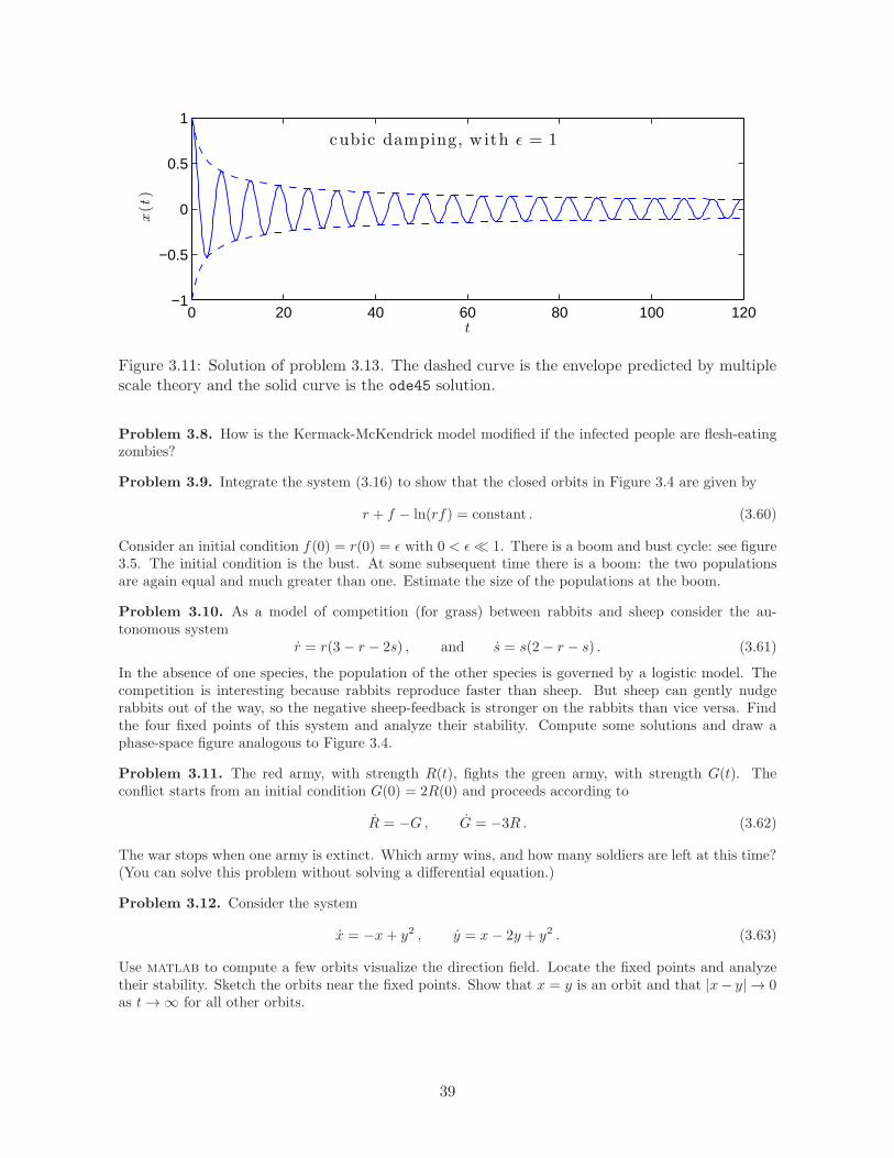
Figure 3.11: Solution of problem 3.13. The dashed curve is the envelope predicted by multiplescale theory and the solid curve is the ode45 solution.

Problem 3.8. How is the Kermack-McKendrick model modified if the infected people are flesh-eatingzombies?

Problem 3.9. Integrate the system (3.16) to show that the closed orbits in Figure 3.4 are given by

r + f − ln(rf) = constant . (3.60)

Consider an initial condition f(0) = r(0) = ǫ with 0 < ǫ≪ 1. There is a boom and bust cycle: see figure3.5. The initial condition is the bust. At some subsequent time there is a boom: the two populationsare again equal and much greater than one. Estimate the size of the populations at the boom.

Problem 3.10. As a model of competition (for grass) between rabbits and sheep consider the au-tonomous system

r = r(3 − r − 2s) , and s = s(2− r − s) . (3.61)

In the absence of one species, the population of the other species is governed by a logistic model. Thecompetition is interesting because rabbits reproduce faster than sheep. But sheep can gently nudgerabbits out of the way, so the negative sheep-feedback is stronger on the rabbits than vice versa. Findthe four fixed points of this system and analyze their stability. Compute some solutions and draw aphase-space figure analogous to Figure 3.4.

Problem 3.11. The red army, with strength R(t), fights the green army, with strength G(t). Theconflict starts from an initial condition G(0) = 2R(0) and proceeds according to

R = −G , G = −3R . (3.62)

The war stops when one army is extinct. Which army wins, and how many soldiers are left at this time?(You can solve this problem without solving a differential equation.)

Problem 3.12. Consider the system

x = −x+ y2 , y = x− 2y + y2 . (3.63)

Use matlab to compute a few orbits visualize the direction field. Locate the fixed points and analyzetheir stability. Sketch the orbits near the fixed points. Show that x = y is an orbit and that |x− y| → 0as t→ ∞ for all other orbits.

39

Problem 3.13. Consider the nonlinearly damped oscillator

x+ ǫx3 + x = 0 , with ICs x(0) = 1 , x(0) = 0 . (3.64)

Assuming that ǫ ≪ 1, use the energy equation and the method of averaging to determine the slowevolution of the amplitude a in the approximate solution (??). Take ǫ = 1 and use ode45 to compare anumerical solution of the cubically damped oscillator with the method of averaging (see Figure 3.11).

Problem 3.14. A theoretically inclined vandal wants to break a steam radiator away from its foun-dation. She steadily applies a force of F = 100Newtons and discovers that the top of the radiator isdisplaced by 2cm. Unfortunately this is only one tenth of the displacement required. But the vandalcan apply an unsteady force f(t) according to the schedule

f(t) = 12F (1− cosωt) , with F = 100N .

The mass of the radiator is 50 kilograms and the foundation resists movement with a force proportionalto displacement. At what frequency and for how long must the vandal exert the force above to succeed?

Problem 3.15. The nonlinear oscillator

x+ x− 2x2 + x3 = 0 , (3.65)

has an energy integral of the formE = 1

2 x2 + V (x) . (3.66)

(i) Find the potential function V (x) and sketch this function on the range − 12 < x < 2. Label your axes

so that your sketch of V (x) is quantitative. (ii) Figure 3.12 shows three possible phase plane diagrams.In ten or twenty words explain which diagram corresponds to the oscillator in (3.65).

Problem 3.16. The top panel in figure 3.13 shows a potential and the bottom panel shows four constantenergy curves in the phase plane. Match the curves in the bottom panel to the indicated energy levels.

40

x

x t

(a)

0 1 2−1

−0.8

−0.6

−0.4

−0.2

0

0.2

0.4

0.6

0.8

1

x

(b)

0 1 2−1

−0.8

−0.6

−0.4

−0.2

0

0.2

0.4

0.6

0.8

1

x

(c)

0 1 2−1

−0.8

−0.6

−0.4

−0.2

0

0.2

0.4

0.6

0.8

1

Figure 3.12: Which phase-plane corresponds to (3.65)?

−6 −4 −2 0 2 4 6

−0.4

−0.2

0

0.2

x

U(x

)

E = [−0 .4 , −0 .2 , 0 .0495 , 0 .205]

x

x

−6 −4 −2 0 2 4 6−2

−1

0

1

2

Figure 3.13: Match the curves to the energy level.

41

Lecture 4

Regular perturbation of ordinary

differential equations

4.1 Initial value problems: the projectile problem

If one projects a particle vertically upwards from the surface of the Earth at z = 0 with speed u then theprojectile reaches a maximum height h = u2/2g0 and returns to the ground at t = 2u/g0 (ignoring airresistance). At least that’s what happens if the gravitational acceleration g0 is constant. But a bettermodel is that the gravitational acceleration is

g(z) =g0

(1 + z/R)2,

where g0 = 9.8m s−2, R = 6, 400kilometers and z is the altitude. The particle stays aloft longer than2u/g0 because gravity is weaker up there.

Let’s use perturbation theory to calculate the correction to the time aloft due to the small decrease inthe force of gravity. But first, before the perturbation expansion, we begin with a complete formulationof the problem. We must solve the second-order autonomous differential equation

d2z

dt2= − g0

(1 + z/R)2, (4.1)

with the initial condition

t = 0 : z = 0 anddz

dt= u . (4.2)

We require the time τ at which z(τ) = 0. Notice that if R = ∞ we recover the elementary problem withuniform gravity.

An important part of this problem is non-dimensionalizing and identifying the small parameter usedto organize a perturbation expansion. We use the elementary problem (R = ∞) to motivate the followingdefinition of non-dimensional variables

zdef=

g0z

u2, and t

def=

g0t

u. (4.3)

Notice thatd

dt=g0u

d

dt, and therefore

d2z

dt2=(g0u

)2 d2

dt2u2

g0z = g0

d2z

dt2(4.4)

Putting these expressions into (4.1) we obtain the non-dimensional problem

d2z

dt2+

1

(1 + ǫz)2= 0 , (4.5)

42

where

ǫdef=

u2

Rg0. (4.6)

We must also non-dimensionalize the initial conditions in (4.2):

t = 0 : z = 0 anddz

dt= 1 . (4.7)

At this point we have done nothing more than change notation. The original problem was specified bythree parameters, g0, u and u. The non-dimensional problem is specified by a single parameter ǫ, whichmight be large, small, or in between. If we’re interested in balls and bullets fired from the surface of theEarth then ǫ≪ 1.

OK, so assuming that ǫ ≪ 1 we try a regular perturbation expansion on (4.5). We also drop allthe bars that decorate the non-dimensional variables: we can restore the dimensions at the end of thecalculation and it is just too onerous to keep writing all those little bars. The regular perturbationexpansion is

z(t) = z0(t) + ǫz1(t) + ǫ2z2(t) + ord(ǫ3). (4.8)

We use the binomial theorem

(1 + x)n = 1 + nx+n(n− 1)

2x2 + ord

(x3), (4.9)

with n = −2 to expand the nonlinear term:

(1 + ǫz)−2 = 1− 2ǫz + 3ǫz2 + ord(ǫ3). (4.10)

Introducing (4.8) into the expansion above gives

(1 + ǫz)−2 = 1− 2ǫz0 + ǫ2(3z20 − 2z1) + ord(ǫ3). (4.11)

So matching up equal powers of ǫ in (4.5) (and denoting time derivatives by dots) we obtain the firstthree terms in perturbation hierarchy:

z0 = −1 , with z0(0) = 0 , z0(0) = 1 ,

z1 = 2z0 , with z1(0) = 0 , z1(0) = 0 ,

z2 = 2z1 − 3z20 , with z2(0) = 0 , z2(0) = 0 .

Above we have the first three terms in a hierarchy of linear equations of the form

Lzn+1 = R(z0, · · · zn) , (4.12)

where the linear operator is

Ldef=

d2

dt2. (4.13)

To solve each term in the hirerarchy we must invert this linear operator, being careful to use the correctinitial equations that zn+1(0) = zn+1(0) = 0.

The solution of the first two equations is

z0(t) = t− t2

2, and z1(t) =

t3

3− t4

12. (4.14)

To obtain z2(t) we integrate

z2 = −3t2 +11t3

3− 11t4

12, (4.15)

to obtain

z2(t) = − t4

4+

11t5

60− 11t6

360. (4.16)

43

Thus the expanded solution is

z(t) = t− t2

2+ ǫ

(t3

3− t4

12

)

+ ǫ2(

− t4

4+

11t5

60− 11t6

360

)

+ ord(ǫ3). (4.17)

We assume that the time aloft, τ(ǫ), also has a perturbation expansion

τ(ǫ) = τ0 + ǫτ1 + ǫ2τ2 + ord(ǫ3). (4.18)

The terms in this expansion are determined by solving:

z0(τ0 + ǫτ1 + ǫ2τ2

)+ ǫz1 (τ0 + ǫτ1) + ǫ2z2 (τ0) = ord

(ǫ3). (4.19)

We have ruthlessly ditched all terms of order ǫ3 into the garbage heap on the right of (4.19). The leftside is a polynomial of order τ6 so there are six roots. One of these roots is τ = 0 and another root isclose to τ = 2. The other four roots are artificial creatures of the perturbation expansion and should beignored — if we want the time aloft then we focus on the root near τ = 2 by taking τ0 = 2 in (4.18).Expanding the zn’s in a Taylor series about τ0 = 2, we have:

z0(2) + (ǫτ1 + ǫ2τ2)z0(2) +12 (ǫτ1)

2z0(2) + ǫz1(2) + ǫ2τ1z1(2) + ǫ2z2(2) = ord(ǫ3). (4.20)

Now we can match up powers of ǫ:

z0(2) = 0 ,

τ1z0(2) + z1(2) = 0 ,

τ2z0(2) +12τ

21 z0(2) + τ1z1(2) + z2(2) = 0 .

Solving1 these equations, one finds

τ = 2 +4

3ǫ+

4

5ǫ2 + ord(ǫ3) .

The Taylor series above is another procedure for generating the expansion of a regularly perturbed rootof a polynomial.

Attempted solution of the projectile problem by iteration

We’re considering the differential equation

d2z

dt2+

1

(1 + ǫz)2= 0 , (4.21)

again. Our first iterate is

z(0) = t− t2

2, (4.22)

which is the same as the first term in the earlier RPS. To obtain the next iterate, z(1)(t), we try to solve

d2z(1)

dt2+

1(1 + ǫ

(t− t2

2

))2 = 0 , (4.23)

with the initial conditionz(1) = 0 , z(1)(0) = 1 . (4.24)

We could assault this problem with mathematica:

DSolve[z’’[t] + 1/(1 + (t - t^2/2))^2 == 0 , z[0] == 0 , z’[0] == 1, z[t], t]

However the answer is not presentable in polite company. In this example, the RPS back in (4.17) isdefinitely superior to iteration.

1Some intermediate results z0(2) = −1, z1(2) = 4/3, z1(2) = 4/3 and z2(2) = −4/45.

44

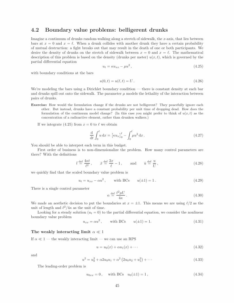
4.2 Boundary value problems: belligerent drunks

Imagine a continuum of drunks random-walking along a stretch of sidewalk, the x-axis, that lies betweenbars at x = 0 and x = ℓ. When a drunk collides with another drunk they have a certain probabilityof mutual destruction: a fight breaks out that may result in the death of one or both participants. Wedesire the density of drunks on the stretch of sidewalk between x = 0 and x = ℓ. The mathematicaldescription of this problem is based on the density (drunks per meter) u(x, t), which is governed by thepartial differential equation

ut = κuxx − µu2 , (4.25)

with boundary conditions at the bars

u(0, t) = u(ℓ, t) = U . (4.26)

We’re modeling the bars using a Dirichlet boundary condition — there is constant density at each barand drunks spill out onto the sidewalk. The parameter µ models the lethality of the interaction betweenpairs of drunks.

Exercise: How would the formulation change if the drunks are not belligerent? They peacefully ignore eachother. But instead, drunks have a constant probability per unit time of dropping dead. How does theformulation of the continuum model change? (In this case you might prefer to think of u(x, t) as theconcentration of a radioactive element, rather than drunken walkers.)

If we integrate (4.25) from x = 0 to ℓ we obtain

d

dt

∫ ℓ

0

u dx =[κux

]ℓ

0−∫ ℓ

0

µu2 dx . (4.27)

You should be able to interpret each term in this budget.First order of business is to non-dimensionalize the problem. How many control parameters are

there? With the definitions

tdef=

4κt

ℓ2, x

def=

2x

ℓ− 1 , and u

def=

u

U, (4.28)

we quickly find that the scaled boundary value problem is

ut = uxx − αu2 , with BCs u(±1) = 1 . (4.29)

There is a single control parameter

αdef=

ℓ2µU

4κ. (4.30)

We made an aesthetic decision to put the boundaries at x = ±1. This means we are using ℓ/2 as theunit of length and ℓ2/4κ as the unit of time.

Looking for a steady solution (ut = 0) to the partial differential equation, we consider the nonlinearboundary value problem

uxx = αu2 , with BCs u(±1) = 1. (4.31)

The weakly interacting limit α≪ 1

If α≪ 1 — the weakly interacting limit — we can use an RPS

u = u0(x) + αu1(x) + · · · (4.32)

andu2 = u20 + α2u0u1 + α2

(2u0u2 + u21

)+ · · · (4.33)

The leading-order problem is

u0xx = 0 , with BCs u0(±1) = 1 , (4.34)

45

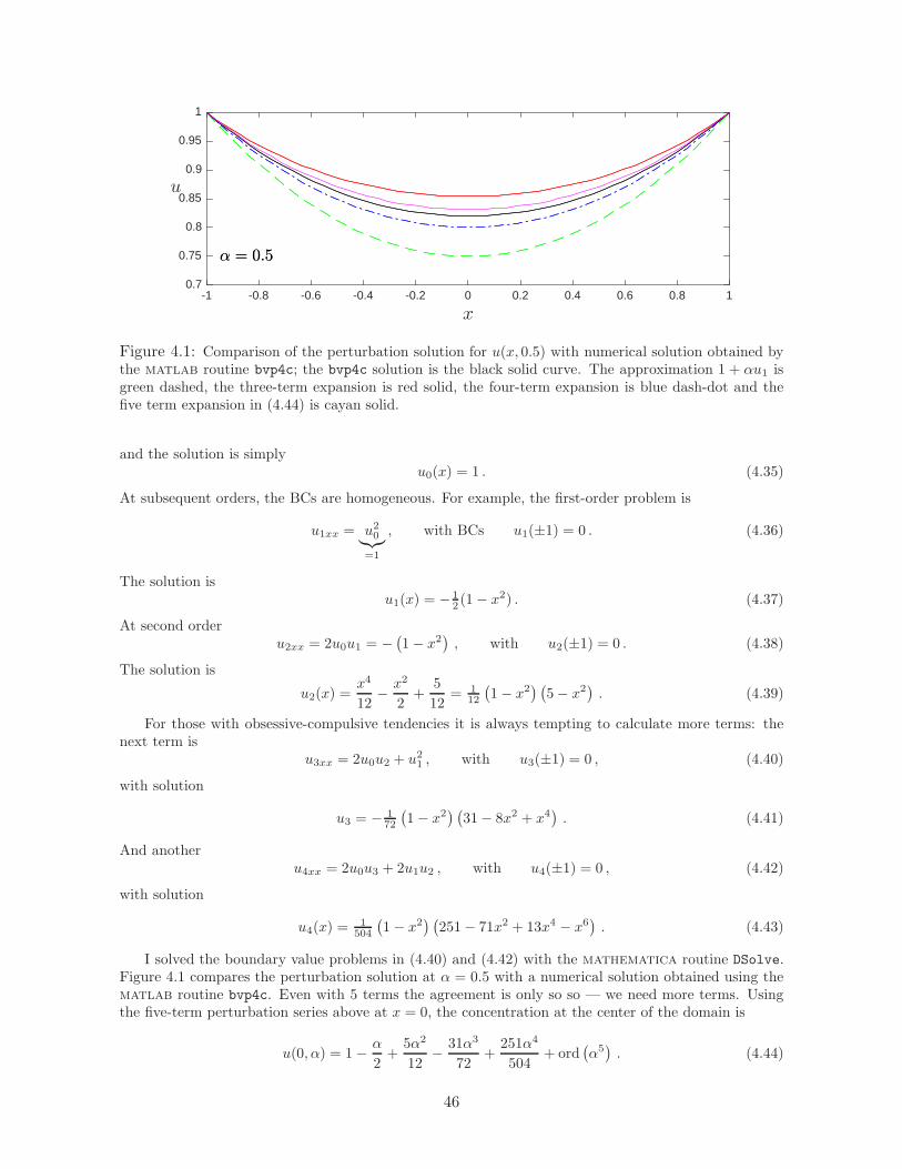
-1 -0.8 -0.6 -0.4 -0.2 0 0.2 0.4 0.6 0.8 1

x

0.7

0.75

0.8

0.85

0.9

0.95

1

u

α = 0.5α = 0.5

Figure 4.1: Comparison of the perturbation solution for u(x, 0.5) with numerical solution obtained bythe matlab routine bvp4c; the bvp4c solution is the black solid curve. The approximation 1 + αu1 isgreen dashed, the three-term expansion is red solid, the four-term expansion is blue dash-dot and thefive term expansion in (4.44) is cayan solid.

and the solution is simplyu0(x) = 1 . (4.35)

At subsequent orders, the BCs are homogeneous. For example, the first-order problem is

u1xx = u20︸︷︷︸

=1

, with BCs u1(±1) = 0 . (4.36)

The solution isu1(x) = − 1

2 (1− x2) . (4.37)

At second orderu2xx = 2u0u1 = −

(1− x2

), with u2(±1) = 0 . (4.38)

The solution is

u2(x) =x4

12− x2

2+

5

12= 1

12

(1− x2

) (5− x2

). (4.39)

For those with obsessive-compulsive tendencies it is always tempting to calculate more terms: thenext term is

u3xx = 2u0u2 + u21 , with u3(±1) = 0 , (4.40)

with solution

u3 = − 172

(1− x2

) (31− 8x2 + x4

). (4.41)

And anotheru4xx = 2u0u3 + 2u1u2 , with u4(±1) = 0 , (4.42)

with solution

u4(x) =1

504

(1− x2

) (251− 71x2 + 13x4 − x6

). (4.43)

I solved the boundary value problems in (4.40) and (4.42) with the mathematica routine DSolve.Figure 4.1 compares the perturbation solution at α = 0.5 with a numerical solution obtained using thematlab routine bvp4c. Even with 5 terms the agreement is only so so — we need more terms. Usingthe five-term perturbation series above at x = 0, the concentration at the center of the domain is

u(0, α) = 1− α

2+

5α2

12− 31α3

72+

251α4

504+ ord

(α5). (4.44)

46

0 5 10

α

0.3

0.4

0.5

0.6

0.7

0.8

0.9

c

0 0.5 1

α

0.7

0.75

0.8

0.85

0.9

0.95

1

c

11 te

rms

6 terms

2 terms

3 terms

Figure 4.2: In both panels the solid black curve is c(α) defined implicitly by (4.49); the integral isevaluated with the matlab routine integral. In the left panel the implicit solution is compared withthe α → ∞ approximation in (4.53). In the right panel the implicit solution is compared to the seriesin (4.57).

We extend this series below in (4.57)At every step of the perturbation hierarchy we are inverting the linear operator d2/dx2 with homo-

geneous Dirichlet boundary conditions. You should recognize that all the regular perturbation problemswe’ve seen have this structure. There is a general result — the implicit function theorem — whichassures us that if we know how to solve these reduced linear problems, with invertible linear operators,then the original problem has a solution for some sufficiently small value of the expansion parameter (αin the problem above).

Example: Let’s consider a different approach to solving the boundary value problem

uxx = αu2 , with BCs u(±1) = 1 . (4.45)

Following our discussion of energy conservation for nonlinear oscillators, we multiplying the equation byux and integrate to obtain

12u2x = α

3u3 + constant . (4.46)

Let c(α)def= u(0, α) be the unknown concentration at the center of the domain, where ux(0, α) = 0.

Evaluating the equation above at x = 0 we see that the constant of integration is −αc3/3. Next, take thesquare root, separate the variables and integrate from x′ = 0 to x > 0 to obtain

∫ u

c

du′√u′3 − c3

=

√

2α

3x . (4.47)

(Notice we take the positive square root because if x > 0 then ux > 0.) Evaluating (4.47) at x = 1 weobtain

∫ 1

c

du′√u′3 − c3

=

√

2α

3. (4.48)

Tidy up by changing variables to v = u′/c:

√

2αc

3=

∫ c−1

1

dv√v3 − 1

. (4.49)

The expression in (4.49) is convenient for numerical work: we can graph the relation between c and α byspecifying c in the range 0 < c < 1 and evaluating α by numerical quadrature (see figure 4.2). Note it isnot necessary to use fzero.

The form in (4.49) is useful in the limit α→ ∞ and c→ 0: an asymptotic approximation to c is obtained

47

by

√

2αc

3=

∫ ∞

1

dv√v3 − 1

−∫ ∞

c−1

dv√v3 − 1

, (4.50)

≈ 2√πΓ (7/6)

Γ (2/3)−∫ ∞

c−1

dv

v3/2, (4.51)

= 2√πΓ (7/6)

Γ (2/3)︸ ︷︷ ︸

=2.42865

−2√c . (4.52)

Solving (4.52) for c, we obtain the approximation

c ∼(

2.42865

2 +√

2α/3

)2

, as α→ ∞. (4.53)

The left panel of figure 4.2 compares this approximation with the result from numerical evaluation of theintegral in (4.49).

Note I have written ∼ in (4.52) — this is unjustified because I haven’t displayed the asymptotic sequenceused to construct the approximation, nor indicated how one might obtain more terms. On the other hand,the large-α comparison with the “exact” solution is splendid — careful justification of the approximation(4.53) seems pointless.

One can also use (4.49) to reproduce and extend the α→ 0 approximation in (4.44). Changing variablesto w = v − 1:

√2αc =

∫ f

0

dw

w

(1 + w + 1

3w2)−1/2

, (4.54)

where fdef= c−1 − 1 ≪ 1. Using mathematica

√2αc =

∫ f

0

dw

w

(

1− w

2+

5w2

24+ · · ·

)

, (4.55)

= 2f1/2 − f3/2

3+f5/2

12+ · · · (4.56)

Squaring the expression above and using InverseSeries to express c in terms of α one eventually arrivesat

c = 1− α

2+

5α2

12− 31α3

72+

251α4

504− 5599α5

9072+

43615α6

54432− 10657285 α7

9906624

+25157603 α8

16982784− 4452284365 α9

2139830784+

241448268505 α10

81313569792+O

(α11). (4.57)

The coefficients are growing slowly — this series may have a non-zero radius of convergence. The rightpanel of figure 4.2 compares partial sums of (4.57) to the exact solution. This example is frustrating: thefunction c(α) is only slightly bent in the range 0 ≤ α ≤ 1. Yet the series (4.57) is ineffective beyond aboutα = 0.5. This may be a job for Pade summation.

4.3 Failure of RPS: singular perturbation problems

Let’s close by giving a few examples of differential equation that do not obligingly yield to regularperturbation methods.

Boundary layers

First, consider the boundary value problem (4.31) with α = ǫ−1 ≫ 1. In terms of ǫ, the problem is

ǫuxx = u2 , with BCs u(±1) = 1 . (4.58)

We try the RPSu = u0(x) + ǫu1(x) + · · · (4.59)

48

The leading order is0 = u20 , with BCs u0(±1) = 1 . (4.60)

Immediately we see that there is no solution to the leading-order problem.What’s gone wrong? Let’s consider a linear problem with the same issues:

ǫvxx = v , with BCs v(±1) = 1 . (4.61)

Again the RPS fails because the leading-order problem,

0 = v0 , with BCs v0(±1) = 1 , (4.62)

has no solution. The advantage of a linear example is that we can exhibit the exact solution:

v =cosh(x/

√ǫ)

cosh(1/√ǫ), (4.63)

see figure 4.3(a). The exact solution has boundary layers near x = −1 and x = +1. In these regionsv varies rapidly so that the term ǫvxx in (4.61) is not small relative to v. Note that the leading orderinterior solution, v0 = 0 is a good approximation to the correct solution outside the boundary layers. Inthis interior region the exact solution is exponentially small e.g.,

v(0, ǫ) =1

cosh(1/√ǫ)

∼ 2e−1/√ǫ , as ǫ→ 0. (4.64)

Our attempted RPS is using ǫn as gauge functions and as ǫ→ 0

2e−1/√ǫ = O (ǫn) , for all n ≥ 0. (4.65)

As far as the ǫn gauge is concerned, e−1/√ǫ is indistinguishable from zero.

The problem in both the examples above is that the small parameter ǫ multiplies the term with themost derivatives. Thus the leading-order problem in the RPS is of lower order than the exact problem.In fact, in the examples above, the leading-order problem is not even a differential equation.

Rapid oscillations

Another linear problem that defeats a regular perturbation expansion is

ǫwxx = −w , with BCs w(±1) = 1 . (4.66)

The exact solution, shown in figure 4.3(b), is

w =cos(x/

√ǫ)

cos(1√ǫ)

. (4.67)

In this case the solution is rapidly varying throughout the domain. The term ǫwxx is never smaller thanw.

Secular errors

Let’s consider a more subtle problem:

x+ (1 + ǫ)x = 0 , with ICs x(0) = 1 , and x(0) = 0 . (4.68)

The exact solution of this oscillator problem is

x(t, ǫ) = cos(√

1 + ǫ t). (4.69)

49

0 10 20 30 40 50 60 70 80 90t

-1

0

1

x(t)

(c) ǫ = 0.05

-1 -0.5 0 0.5 1x

0

0.5

1

v(x,ǫ)

(a) ǫ = 0.004

-1 -0.5 0 0.5 1x

-1

0

1

w(x,ǫ)

(b) ǫ = 0.004

0 10 20 30 40 50 60 70 80 90t

-2

0

2

x(t)

(d) ǫ = 0.05

Figure 4.3: ??????

s

50

In this case it looks like the RPS

x(t, ǫ) = x0(t) + ǫx1(t) + ǫ2x2(t) + · · · (4.70)

might work. The leading-order problem is

x0 + x0 = 0 , with ICs x0(0) = 1 , and x0(0) = 0 , (4.71)

with solutionx0 = cos t . (4.72)

In fact, this RPS does work for some time — see figure 4.3(c). But eventually the exact solution (4.69)and the leading-order approximation in (4.72) have different signs. That’s a bad error if x0(t) is a clock.

Maybe we can improve the approximation by calculating the next term? The order ǫ1 problem is

x1 + x1 = − cos t , (4.73)

with homogeneous initial conditions

x1(0) = 0 , and x1(0) = 0 . (4.74)

I hope you recognize a resonantly forced oscillator when you see it: the solution of (4.73) is

x1 = − 12 t sin t . (4.75)

Thus the perturbation solution is now

x = cos t− ǫ 12 t sin t+ ord(ǫ2). (4.76)

This first-order “correction” makes matters worse — see figure 4.3(d). The RPS in (4.76) is “disordered”once ǫt = ord(1): we don’t expect an RPS to work if the higher order terms are larger than the earlierterms. Clearly there is a problem with direct perturbative solution of an elementary problem.

In this example the term ǫx is small relative to the other two terms in differential equation at alltime. Yet the small error slowly accumulates over long times ∼ ǫ−1. Astronomers call this a secularerror2. We did not face secular errors in the projectile problem because we were solving the differentialequation only for the time aloft, which was always much less than 1/ǫ.

2From Latin saecula, meaning a long period of time. Saecula saeculorum is translated literally as “in a centuryof centuries”, or more poetically as “forever and ever”, or “world without end”.

51

4.4 Problems

Problem 4.1. (i) Consider the projectile problem with linear drag:

d2z

dt2+ µ

dz

dt= −g0 , (4.77)

and the initial conditions z(0) = 0 and dz/dt = u. Find the solution with no drag, µ = 0, and calculatethe time aloft, τ . (ii) Suppose that the drag is small — make this precise by non-dimensionalizingthe equation of motion and exhibiting the relevant small parameter ǫ. (iii) Use a regular perturbationexpansion to determine the first correction to τ associated with non-zero drag. (iv) Integrate the non-dimensional differential equation exactly and obtain a transcendental equation for τ(ǫ). Asymptoticallysolve this transcendental equation approximately in the limits ǫ → 0 and ǫ → ∞. Make sure the ǫ → 0solution agrees with the earlier RPS.

Problem 4.2. Consider the projectile problem with quadratic drag:

d2z

dt2+ ν∣∣∣dz

dt

∣∣∣dz

dt= −g0 , (4.78)

and the initial conditions z(0) = 0 and dz/dt = u. (i) Explain why the absolute value |z| in (4.78)is necessary if this term is to model air resistance. (ii) What are the dimensions of the coefficient ν?Nondimensionalize the problem so there is only one control parameter. (iii) Suppose that ν is small.Use a regular perturbation expansion to determine the first correction to the time aloft. (iv) Solve thenonlinear problem exactly and obtain a transcendental equation for the time aloft. (This is complicated.)

Problem 4.3. In this problem we use energy conservation to obtain a solution to the projectile problemwhich is superior to (4.17). (i) From the non-dimensional equation of motion (4.5), show that

12 z

2 − 1

ǫ

1

1 + ǫz= 1

2 − 1

ǫ. (4.79)

(ii) Find the maximum height reached by the projectile, zmax, in terms of ǫ. (iii) Show that the timealoft is given exactly by

τ = 2zmax

∫ 1

0

√

1 + aξ

1− ξdξ , with a(ǫ)

def=

ǫ

2− ǫ. (4.80)

(iv) Evaluate the integral above exactly. (e) Use mathematica or some other tool to obtain the ǫ≪ 1expansions

τ =4

2− ǫ

[

1 +a

3− a2

15+a3

35− a4

63+a5

99− a6

143+ ord

(a7)]

. (4.81)

and

τ = 2 +4ǫ

3+

4ǫ2

5+

16ǫ3

35+

16ǫ4

63+

32ǫ5

231+

32ǫ6

429+ ord

(ǫ7). (4.82)

Which series is superior at ǫ = 0.5?

Problem 4.4. (i) Solve the problem

x+(1 + ǫeαt

)x = 0 , with IC x(0, ǫ, α) = 1 , x(0, ǫ, α) = 0 , (4.83)

with the RPSx(t, ǫ, α) = x0(t, α) + ǫx1(t, α) + · · · (4.84)

Calculate x0 and x1. (ii) Bearing in mind that α might be positive or negative, discuss the utility of theRPS when t is large.

52

0 5 10 15 20 250

0.5

1

1.5

Figure 4.4: Numerical solution of (4.85) with various initial conditions. In this illustrationK1/K0 = 0.1 and ω/r = 2. At large time all initial conditions convergence to a periodicsolution that lags the carrying capacity.

Problem 4.5. Consider the logistic equation with a periodically varying carrying capacity:

N = rN

(

1− N

K

)

, with K = K0 +K1 cosωt . (4.85)

The initial condition is N(0) = N0. (i) Based on the K1 = 0 solution, non-dimensionalize this problem.Show that there are three control parameters. (ii) Suppose that K1 is a perturbation i.e., K1/K0 ≪ 1.The numerical solution in Figure 4.4 shows that eventually the initial condition is “forgotten” and allsolutions converge to a periodic oscillation about the mean carrying capacity K0. Use perturbationtheory to determine the amplitude and phase of the long-term oscillation.

Problem 4.6. Consider a partial differential equation analog to the boundary value problem in (4.31).

The domain is the disc r =√

x2 + y2 < a in the (x, y)-plane and the problem is

uxx + uyy = αu2 , with BC: u(a, θ) = U . (4.86)

Following the discussion in section 4.2, compute three terms in the RPS.

Problem 4.7. Let’s make a small change to the formulation of the belligerent-drunks example in (4.25)and (4.26). Suppose that we model the bars using a Neumann boundary condition. This means thatthe flux of drunks, rather than the concentration, is prescribed at x = 0 and ℓ: the boundary conditionin (4.26) is changed to

κux(0, t) = −F , and κux(ℓ, t) = F , (4.87)

where F , with dimensions drunks per second, is the flux entering the domain from the bars. Try torepeat all calculations in section 4.2, including the analog of the β ≪ 1 perturbation expansion. You’llfind that it is not straightforward and that a certain amount of ingenuity is required to understand theweakly interacting limit with fixed-flux boundary conditions.

Problem 4.8. First read the section entitled Boundary layers. Inspired by the example in thatsection, find an approximate solution of the boundary value problem:

10−12vxx = ex4

v , with BCs v(±1) = 1 . (4.88)

If you can do this, you’ll be on on your way to understanding boundary layer theory.

Problem 4.9. Consider the non-dimensional oscillator problem

x+ βx+ x = 0 , (4.89)

with the initial conditionsx(0) = 0 , and x(0) = 1 . (4.90)

53

(i) Supposing that β > 2, solve the problem exactly. (ii) Show that if β ≫ 1 then the long-timebehaviour of your exact solution is

x ∝ e−t/β , (4.91)

i.e., the displacement very slowly decays to zero. (iii) Motivated by this exact solution, “rescale” theproblem (and the initial condition) by defining the slow time

τdef=

t

β, (4.92)

and X(τ) =?x(t). Show that with a suitable choice of ?, the rescaled problem is

ǫXττ +Xτ +X = 0 with the IC: X(0) = 0 , Xτ (0) = 1 . (4.93)

Make sure you give the definition of X(τ) and ǫ ≪ 1 in terms of the parameter β ≫ 1 and the originalvariable x(t). (iv) Try to solve the rescaled problem (4.93) using an RPS

X(τ, ǫ) = X0(τ) + ǫX1(τ) + · · · (4.94)

Discuss the miserable failure of this approach by analyzing the dependence of the exact solution frompart (i) on β. That is, simplify the exact solution to deduce a useful β → ∞ approximation, and explainwhy the RPS (4.94) cannot provide this useful approximation.

Problem 4.10. Consider a medium −ℓ < x < ℓ in which the temperature θ(x, t) is determined by

θt − κθxx = αeβθ , (4.95)

with boundary conditions θ(±ℓ, t) = 0. The right hand side is a heat source due to an exothermicchemical reaction. The simple form in (4.95) is obtained by linearizing the Arrhenius law. The mediumis cooled by the cold walls at x = ±ℓ. (i) Put the problem into the non-dimensional form

ΘT −ΘXX = ǫeΘ with BCs Θ(±1, ǫ) = 0 . (4.96)

Your answer should include a definition of the dimensionless control parameter ǫ in terms of κ, α, βand ℓ. (ii) Assuming that ǫ ≪ 1, calculate the steady solution Θ(X, ǫ) using a regular perturbationexpansion. Obtain two or three non-zero terms and check your answer by showing that the “centraltemperature” is

C(ǫ)def= Θ(0, ǫ) , (4.97)

=ǫ

2+

5ǫ2

24+

47ǫ3

360+ ord

(ǫ4). (4.98)

(iii) Develop an approximate solution with iteration. (iv) Integrate the steady version of (4.96) exactlyand deduce that:

e−C/2 tanh−1√

1− e−C︸ ︷︷ ︸

def=F (C)

=

√ǫ

2. (4.99)

(Use mathematica to do the integral.) Plot the function F (C) and show that there is no steady solutionif ǫ > 0.878. (v) Based on the graph of F (C), if ǫ < 0.878 then there are two solutions. There is the“cold solution”, calculated perturbatively in (4.98), and there is a second “hot solution” with a largecentral temperature. Find an asymptotic expression for the hot central temperature as ǫ→ 0.

54

Lecture 5

Regular perturbation of partial

differential equations

Let’s consider some perturbation problems presented by partial differential equations — a main noveltyis perturbation of geometry.

5.1 Thermal diffusion in solids

We’ll use the diffusion equation as a main example. The conservation law for energy in a solid withnon-uniform temperature is

Qt +∇·F = 0 , (5.1)

where the heat content and energy flux are

Q = ρcT , and F = −κ∇T . (5.2)

Above T is the temperature (K), c is the heat capacity (J/K kg), ρ is the density (kg/m3) and and κ isthe conductivity. Assuming that c, ρ and κ are all constant, (5.1) is rewritten as the diffusion equation

Tt = κ∇2T , (5.3)

where κdef= κ/ρc is the thermal diffusivity and ∇2 is the laplacian operator.

5.2 Steady heat diffusion through a corrugated slab

The simplest problem is steady thermal diffusion through a slab of thickness H . Suppose that thebottom face at z = 0 is held at temperature T0 and the top face at z = H is held at T0 +∆T . Then insteady state (5.3) collapses to

κTzz = 0 . (5.4)

With the boundary conditions stated above the solution is

T = T0 +∆T z

H. (5.5)

The heat flux through the slab is

F = −κ∆T

Hz , (5.6)

with dimensions W/m2.

55

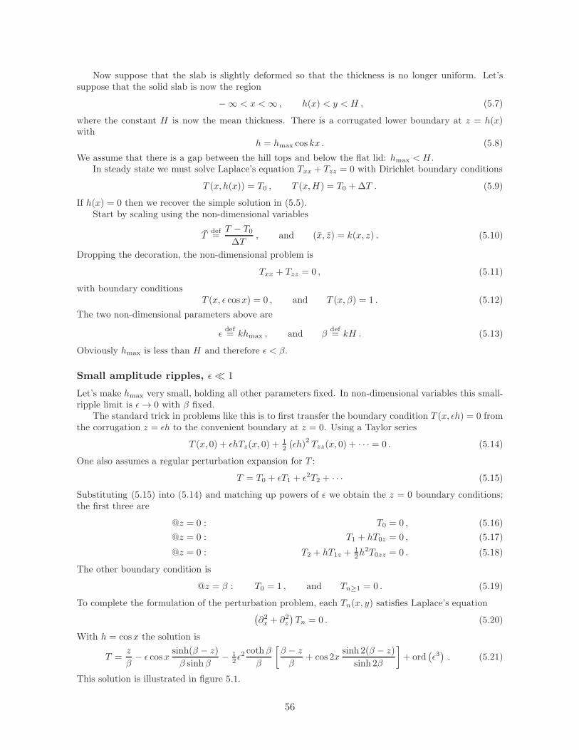
Now suppose that the slab is slightly deformed so that the thickness is no longer uniform. Let’ssuppose that the solid slab is now the region

−∞ < x <∞ , h(x) < y < H , (5.7)

where the constant H is now the mean thickness. There is a corrugated lower boundary at z = h(x)with

h = hmax cos kx . (5.8)

We assume that there is a gap between the hill tops and below the flat lid: hmax < H .In steady state we must solve Laplace’s equation Txx + Tzz = 0 with Dirichlet boundary conditions

T (x, h(x)) = T0 , T (x,H) = T0 +∆T . (5.9)

If h(x) = 0 then we recover the simple solution in (5.5).Start by scaling using the non-dimensional variables

Tdef=

T − T0∆T

, and (x, z) = k(x, z) . (5.10)

Dropping the decoration, the non-dimensional problem is

Txx + Tzz = 0 , (5.11)

with boundary conditionsT (x, ǫ cosx) = 0 , and T (x, β) = 1 . (5.12)

The two non-dimensional parameters above are

ǫdef= khmax , and β

def= kH . (5.13)

Obviously hmax is less than H and therefore ǫ < β.

Small amplitude ripples, ǫ≪ 1

Let’s make hmax very small, holding all other parameters fixed. In non-dimensional variables this small-ripple limit is ǫ→ 0 with β fixed.

The standard trick in problems like this is to first transfer the boundary condition T (x, ǫh) = 0 fromthe corrugation z = ǫh to the convenient boundary at z = 0. Using a Taylor series

T (x, 0) + ǫhTz(x, 0) +12 (ǫh)

2Tzz(x, 0) + · · · = 0 . (5.14)

One also assumes a regular perturbation expansion for T :

T = T0 + ǫT1 + ǫ2T2 + · · · (5.15)

Substituting (5.15) into (5.14) and matching up powers of ǫ we obtain the z = 0 boundary conditions;the first three are

@z = 0 : T0 = 0 , (5.16)

@z = 0 : T1 + hT0z = 0 , (5.17)

@z = 0 : T2 + hT1z +12h

2T0zz = 0 . (5.18)

The other boundary condition is

@z = β : T0 = 1 , and Tn≥1 = 0 . (5.19)

To complete the formulation of the perturbation problem, each Tn(x, y) satisfies Laplace’s equation(∂2x + ∂2z

)Tn = 0 . (5.20)

With h = cosx the solution is

T =z

β− ǫ cosx

sinh(β − z)

β sinhβ− 1

2ǫ2 cothβ

β

[β − z

β+ cos 2x

sinh 2(β − z)

sinh 2β

]

+ ord(ǫ3). (5.21)

This solution is illustrated in figure 5.1.

56

ǫ = 1/3 and β = 1

-3 -2 -1 0 1 2 3

x

-0.4

-0.2

0

0.2

0.4

0.6

0.8

1

z

Figure 5.1: Contour plot of T in (5.21).

Enhanced heat flux through the corrugated slab

Let’s calculate the heat flux flowing through the corrugated slab. Heat is diffusing in through the hotflat top (z = β) and out through the cold corrugated bottom (z = ǫ cosx). From (5.21), the flux inthrough the flat top at z = β is

Tz(x, β) =1

β+ ǫ

cosx

β sinhβ+ 1

2ǫ2 cothβ

β2

[

1 +2β cos 2x

sinh 2β

]

+ ord(ǫ3). (5.22)

Using 〈〉 to denote an average over the x, the averaged flux through the slab is

〈Tz(x, β)〉 =1

β

(

1 + ǫ2cothβ

2β

)

︸ ︷︷ ︸

def= χ

, (5.23)

where χ is an enhancement factor due to the corrugations. In dimensional variables the heat flux throughthe slab is κ∆Tχ/H (W m−2).

Is it physically intuitive that these corrugations increase the flux of heat through the slab? Onecan argue that the places where the slab is thin (above the hills) are short circuits. This suspicionis confirmed in figure 5.1 which shows that the temperature gradient is increased over the hills anddecreased over the valleys. But this modulation is the order ǫ term in (5.22), which is proportional tocosx and therefore integrates to zero. The flux enhancement χ in (5.23) is order ǫ2 — the big gradientsover the hills more than compensate for the small gradients over the valleys. This effect is subtle and Idon’t have a totally satisfactory physical explanation.

We should also calculate the heat content of the slab

Q(x) =1

2π

∫ π

−π

∫ β

ǫ cosx

T (x, z) dzdx . (5.24)

57

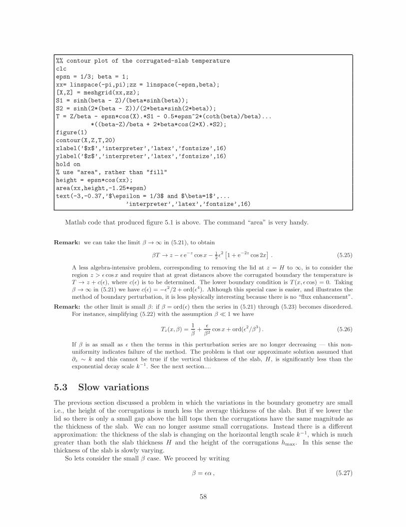
%% contour plot of the corrugated-slab temperature

clc

epsn = 1/3; beta = 1;

xx= linspace(-pi,pi);zz = linspace(-epsn,beta);

[X,Z] = meshgrid(xx,zz);

S1 = sinh(beta - Z)/(beta*sinh(beta));

S2 = sinh(2*(beta - Z))/(2*beta*sinh(2*beta));

T = Z/beta - epsn*cos(X).*S1 - 0.5*epsn^2*(coth(beta)/beta)...

*((beta-Z)/beta + 2*beta*cos(2*X).*S2);

figure(1)

contour(X,Z,T,20)

xlabel(’$x$’,’interpreter’,’latex’,’fontsize’,16)

ylabel(’$z$’,’interpreter’,’latex’,’fontsize’,16)

hold on

% use "area", rather than "fill"

height = epsn*cos(xx);

area(xx,height,-1.25*epsn)

text(-3,-0.37,’$\epsilon = 1/3$ and $\beta=1$’,...

’interpreter’,’latex’,’fontsize’,16)

Matlab code that produced figure 5.1 is above. The command “area” is very handy.

Remark: we can take the limit β → ∞ in (5.21), to obtain

βT → z − ǫ e−z cosx− 12ǫ2[1 + e−2z cos 2x

]. (5.25)

A less algebra-intensive problem, corresponding to removing the lid at z = H to ∞, is to consider theregion z > ǫ cosx and require that at great distances above the corrugated boundary the temperature isT → z + c(ǫ), where c(ǫ) is to be determined. The lower boundary condition is T (x, ǫ cos) = 0. Takingβ → ∞ in (5.21) we have c(ǫ) = −ǫ2/2 + ord(ǫ4). Although this special case is easier, and illustrates themethod of boundary perturbation, it is less physically interesting because there is no “flux enhancement”.

Remark: the other limit is small β: if β = ord(ǫ) then the series in (5.21) through (5.23) becomes disordered.For instance, simplifying (5.22) with the assumption β ≪ 1 we have

Tz(x, β) =1

β+

ǫ

β2cos x+ ord(ǫ2/β3) . (5.26)

If β is as small as ǫ then the terms in this perturbation series are no longer decreasing — this non-uniformity indicates failure of the method. The problem is that our approximate solution assumed that∂z ∼ k and this cannot be true if the vertical thickness of the slab, H , is significantly less than theexponential decay scale k−1. See the next section....

5.3 Slow variations

The previous section discussed a problem in which the variations in the boundary geometry are smalli.e., the height of the corrugations is much less the average thickness of the slab. But if we lower thelid so there is only a small gap above the hill tops then the corrugations have the same magnitude asthe thickness of the slab. We can no longer assume small corrugations. Instead there is a differentapproximation: the thickness of the slab is changing on the horizontal length scale k−1, which is muchgreater than both the slab thickness H and the height of the corrugations hmax. In this sense thethickness of the slab is slowly varying.

So lets consider the small β case. We proceed by writing

β = ǫα , (5.27)

58

where α > 1 and consider the limit ǫ → 0 with α fixed. The thickness-in-z of the slab is now of order ǫeverywhere so it makes sense to “rescale” the vertical coordinate

zdef=

z

ǫ, ⇒ ∂z = ǫ−1∂ζ . (5.28)

The re-scaled problem isǫ2Txx + Tζζ = 0 , (5.29)

with boundary conditionsT (x, cosx) = 0 , and T (x, α) = 1 . (5.30)

Now look for a regular perturbation solution

T = T0(x, ζ) + ǫ2T2(x, ζ) + ord(ǫ4) . (5.31)

The leading-order problem isT0ζζ = 0 , (5.32)

with boundary conditionsT0(x, cos x) = 0 , and T0(x, α) = 1 . (5.33)

Notice that (5.32) is a “one-term dominant balance”. One-term should be simpler than the two-termdominant balances that have figured so prominently in our earlier discussion. But the one-term dominantbalance is subtle: the main point is that (5.32) has a nontrivial general soluton

T0(x, ζ) = A(x) +B(x)ζ . (5.34)

The boundary conditions (5.33) imply that

0 = A+B cosx , and 1 = A+B . (5.35)

Hence the leading-order solution is

T0(x, ζ) =ζ − cosx

α− cosx. (5.36)

We can now calculate the heat flux through the slab....

Example: Poiseuille flow through a tube with slowly changing radius.

5.4 A slowly rotating self-gravitating mass

A mass M of incompressible, self-gravitating and non-rotating fluid, with uniform density ρ, will be inhydrostatic equilibrium as a sphere of radius

rdef=

(3M

4πρ

)1/3

. (5.37)

The gravitational potential is determined by solving

∇2φ = 4πGρχ , (5.38)

where

χ =

1 , inside the mass;

0 , outside the mass.(5.39)

Solving the Poisson equation (5.38), we obtain the well known spherically symmetric solution

φ = −GMr

3r2−r2

2r2 , inside the sphere;rr , outside the sphere .

(5.40)

59

Notice that φ and φr are continuous at r = a; the second derivative is discontinuous at the surface ofthe sphere

φrr(r+)− φrr(r

−) = −3g

r, (5.41)

where the gravitational acceleration at the surface is

gdef=

GM

r2. (5.42)

The liquid mass is in equilibrium because ∇φ is normal to the surface of the sphere. Equivalently, thesurface of the sphere is an equipotential surface.

Solid body rotation, the geopotential and the equilibrium condition

Now suppose that the mass is in slow solid-body rotation about the z-axis with angular velocity Ω = Ωz.The mass is no longer perfectly spherical — the equator is slightly bulged out and the poles are flattened.If we knew the shape of the mass we could determined the potential φ by solving (5.38). Assuming thatthe rotation is weak, and that the deformation from a perfect sphere is small, we proceed to perturbativelysolve (5.38) in combination with the momentum equation.

In solid body rotationu = Ωz × x (5.43)

where x = xx + yy + zz is position relative to the center of mass and u the fluid velocity. Thus theacceleration is

Du

Dt= Ωz × u , (5.44)

= Ω2z × (z × x) , (5.45)

= −Ω2 (xx+ yy) , (5.46)

= −∇12Ω

2(x2 + y2) . (5.47)

The momentum equation,Du

Dt= −∇

(p

ρ+ φ

)

, (5.48)

is therefore equivalent top

ρ+ φ− Ω2 1

2 (x2 + y2) = constant. (5.49)

In (5.49) the gravitational potential φ is obtained from the solution of the Newtonian potential equation(5.38). The effective potential

φ− Ω2 12 (x

2 + y2) (5.50)

in (5.49) is known as the geopotential.The equilibrium condition is that at the unknown surface of the mass the pressure is zero and (5.49)

becomes@r = s(θ) : φ− 1

2Ω2r2 sin2 θ = constant . (5.51)

Above, r = s(θ) is the location of the surface and θ is the usual polar angle in spherical coordinates.Later we need a expression for the unit normal n to the surface. The vector n is proportional to

∇[r − s(θ)], or

n =sr − sθθ√

s2 + s2θ. (5.52)

Thus the normal derivative of the potential, evaluated on the surface of the mass, is

n · ∇φ|r=s︸ ︷︷ ︸

def= φn

=s2φr − sθφθ

s√

s2 + s2θ. (5.53)

The normal derivative above is continuous at the surface.

60

Perturbative solution

Scale analysis identifies a single dimensionless parameter

ǫ =Ω2

ρG=

4π

3

Ω2r

g. (5.54)

“Slow rotation” means that ǫ≪ 1. Instead of non-dimensionalizing the problem and expanding in ǫ, welive dangerously by expanding in terms of the dimensional parameter Ω2:

s = r +Ω2s1(θ) + ord(Ω4), (5.55)

and

φ = −GMr

︸ ︷︷ ︸

φ0

+Ω2φ1 + ord(Ω4). (5.56)

The boundary condition (5.51) is first transferred to r = r via the expansion

φ(s(θ), θ) = φ(r) + (s− r)︸ ︷︷ ︸

=Ω2s1

φr(r, θ) + ord(Ω4). (5.57)

Thus at the convenient boundary

@r = r : φ+Ω2(s1 φr − 1

2 r2 sin2 θ

)+ ord

(Ω4)= constant . (5.58)

The normal derivative in (5.53) is

@r = r : φn = φr(r, s) + Ω2

(

s1φrr −s1θφθr2

)

+ ord(Ω4). (5.59)

The problem for φ1 is therefore∇2φ1 = 0 , (5.60)

with@a : φ1 = −gs1 + 1

2 r2 sin2 θ + constant. (5.61)

In addition, continuity of the normal derivative of φ implies that

φ1r(r+)− φ1r(r

−) = −s1(φ0rr(r

+)− φ0rr(r−))

︸ ︷︷ ︸

=−3g/r

(5.62)

This φ1-problem is forced by12 sin

2 θ = 13 − 1

3P2(θ) (5.63)

where P2(µ) = (3µ2 − 1)/2 is the second Legendre polynomial. Thus we try to solve the φ1-problemwith

s1 = αr P2(cos θ) , (5.64)

and

φ1 = β P2(cos θ)

(r/r)2 , inside the mass;

(r/r)−3 , outside the mass.(5.65)

The construction in (5.65) satisfies Laplace’s equation (5.60) and also continuity of φ1 at the surface.Substituting (5.64) and (5.65) into (5.61) we obtain

β = −rgα− 13 r

2 . (5.66)

Noting that φ1r(r+)− φ1r(r

−) = −5βP2/r, the normal derivative condition in (5.62) gives

5β = −3grα . (5.67)

61

Solving for α and β one obtains

α = −5

6

r

gand β =

r2

2. (5.68)

To summarize, the surface of the mass is r = s(θ) where

s = r − 5

6

r2Ω2

gP2(cos θ) . (5.69)

The polar radius (θ = 0) is

rpol = r − 5

6

r2Ω2

g, (5.70)

and the equatorial radius (θ = π/2) is

req = r +5

12

r2Ω2

g. (5.71)

Thus the “flattening” isreq − rpol

r=

5

4

rΩ2

g. (5.72)

The external potential is

φ = − r2g

r+ P2(cos θ)

Ω2r5

2r3. (5.73)

62

5.5 Problems

Problem 5.1. Consider the partial differential equation

κ (Cxx + Czz)− µC = 0 (5.74)

in the region above z = h(x), with h(x) = hmax cos kx. The boundary conditions are C(x, hmax cos kx) =C∗ and C(x, z) → 0 as z → ∞. (i) Describe a physical situation governed by this boundary value prob-lem. (ii) Solve the problem with hmax = 0. (iii) Based on your exact solution, non-dimensionalize theproblem with non-zero hmax and determine the non-dimensional control parameters. (iv) Use perturba-tion theory to find the first effects of small non-zero hmax on the “inventory”

Adef=

k

2π

∫ ∞

h(x)

∫ 2π/k

0

C(x, z) dxdz . (5.75)

(I think you’ll have to go to second order in hmax.)

Problem 5.2. Consider the diffusion problem

ψxx + ψyy = −e−y (5.76)

in the “corrugated half-plane” defined by

−∞ < x <∞ , and ǫ coskx < y . (5.77)

At the wavy boundary:ψ(x, ǫ cos kx) = 0 . (5.78)

The condition at infinity islimy→∞

ψ(x, y) = A(ǫ, k) , (5.79)

where A(ǫ, k) is an unknown function. (i) Solve the problem with ǫ = 0 and show that A(0, k) = 1. (ii)Use a perturbation expansion (ǫ≪ 1) to determine the first non-zero correction to A = 1.

Problem 5.3. Consider 2D potential flow (no vorticity) around an cylindrical object whose cross sectionin the (x, y)-plane is a slightly distorted circle

r = a(1− ǫ sin2 θ

). (5.80)

Using a stream function ψ(x, y), with u = −ψy and v = ψx, the mathematical problem is

∇2ψ = 0 , (5.81)

where∇2 = ∂2x + ∂2y = ∂2r + r−1∂r + r−2∂2θ (5.82)

is the laplacian operator; boundary conditions are ψ = 0 on the surface of the body and ψ → −Uy atgreat distances from the body. (i) Review the standard solution for potential flow around a circularcylinder i.e., the case ǫ = 0. (This solution is in all fluid mechanics textbooks; above I’m using cylindricalcoordinates r and θ that feature prominently in those textbooks.) (ii) Non-dimensionalize the problemand identify all non-dimensional control parameters. (iii) Use the boundary perturbation method tofind the first effects of small distortion, ǫ≪ 1. Visualize your solution.

Problem 5.4. Consider Laplace’s equation,

φxx + φyy = 0 , (5.83)

in a domain which is a periodic-in-x channel with walls at y = ±(1 + ǫ coskx). The boundary conditionon the walls is

(∇φ+ ı) · n = 0 , (5.84)

where n is the outward normal and ı is the unit vector in the x-direction. Obtain two terms in theexpansion of

J(ǫ)def=

∫∫

φx dxdy . (5.85)

63

kxy

k = 2 and ǫ = 0 .3

0 1 2 3 4 5 6

−1

−0.5

0

0.5

1

kx

y

0 1 2 3 4 5 6

−1.2

−1

−0.8

−0.6

Figure 5.2: My solution to problem 5.5 with k = 2 and ǫ = 0.3. The lower panel is an expandedview of the lower boundary. Some errors in the boundary condition T = 0 are evident nearkx = 0 and 2π. At this largish value of ǫ another term wouldn’t hurt.

Problem 5.5. Consider a uniformly heated 2D metal ribbon of width 2h(x). The ribbon is cooled byfixing T (x, h(x)) = 0 at the two boundaries. Thus the steady state temperature is determined by

Txx + Tyy = −1 , for− h(x) < y < +h(x) , (5.86)

where hdef= 1 + ǫ cos kx. The boundary conditions are

T (x,±h) = 0 . (5.87)

We particularly desire the heat content of the ribbon

J(ǫ, k)def=

k

2π

∫ 2π/k

0

∫ h

−h

T dxdy . (5.88)

Use the boundary perturbation method to show that

J =2

3+ ǫ2 (1− k tanh k) + ord

(ǫ4). (5.89)

64

Lecture 6

Boundary Layers

6.1 Stommel’s dirt pile

Consider a pile of dirt formed by a rain of sediment falling onto a conveyor belt. The belt stretchesbetween x = 0 and x = ℓ and moves to the left with speed −c: see the figure. If h(x, t) denotes theheight of a sandpile, then a very simple model is

ht − chx = s+ κhxx , (6.1)

with boundary conditionsh(0, t) = 0 , and h(ℓ, t) = 0 . (6.2)

The term s(x) on the right of (6.1) is the rate (meters per second) at which sand is falling from the skyonto the belt.

We can make a sanity check by integrating (6.1) from x = 0 to x = ℓ:

d

dt

∫ ℓ

0

h(x, t) dx

︸ ︷︷ ︸

rate of accumulation

=

∫ ℓ

0

s(x, t) dx

︸ ︷︷ ︸

sedimentation from above

+ κhx(ℓ, t)− κhx(0, t)︸ ︷︷ ︸

loss of dirt by falling over the edges

. (6.3)

Notice that the advective term, chx, does not contribute to the budget above — advection is movingdirt but because h = 0 at the boundaries advection is not directly contributing to the fall of dirt overthe edges.

The steady solution with a uniform source

If the sedimentation rate, s(x, t), is a constant then we can easily solve the steady state (t→ ∞) problemexactly:

h(x,∞) =sℓ

c

1− e−cx/κ

1− e−cℓ/κ− sx

c. (6.4)

If the diffusion is very weak, meaning that

ǫdef=

κ

cℓ≪ 1 , (6.5)

then there is a region of rapid variation, the boundary layer, at x = 0. This is where all the sandaccumulated on the conveyor belt is pushed over the edge. Obviously if we reverse the direction of thebelt, then the boundary layer will move to x = ℓ. Note we’re assuming that c > 0 so that ǫ > 0.

If we introduce non-dimensional variables

xdef=

x

ℓ, and h =

ch

sℓ, (6.6)

65

s

-c

z

z = h(x,t)

x

x = ax = 0

Figure 6.1: Stommel’s boundary-layer problem.

0 0.1 0.2 0.3 0.4 0.5 0.6 0.7 0.8 0.9 1x/ℓ

0

0.5

1

ch(x)/sℓ

Figure 6.2: The solution in (6.7). The solid curve is ǫ = 0.1, the dashed curve is ǫ = 0.025 andthe dash-dot curve is ǫ = 0.005.

66

then the solution in (6.4) is

h(x, ǫ) =1− e−x/ǫ

1− e−1/ǫ− x . (6.7)

This solution is shown in figure 6.2. We can consider two different limiting processes

1. The outer limit: ǫ → 0, with x fixed. Under this limit, the exact solution in (6.7) is h → 1 − x.The outer limit produces a good approximation to the exact h(x, ǫ), except close to x = 0 wherethe boundary condition is not satisfied.

2. The inner limit: ǫ → 0 with Xdef= x/ǫ fixed. Under this limit the exact solution in (6.7) is

h→ 1− e−X . The inner limit produces a good approximation to the solution within the boundarylayer. This is a small region in which x is order ǫ. It is vital to understand that the term ǫhxx isleading order within the boundary layer, and enables the solution to satisfy the boundary conditionat x = 0.

Thus the function in (6.7) has two different asymptotic expansions. Each expansion is limited by non-uniformity as ǫ→ 0.

6.2 Leading-order solution of the dirt-pile model

We want to take the inner and outer limits directly in the differential equation, before we have a solution.Understanding how to do this in the Stommel problem is one goal this lecture.

To make the problem a little more interesting, suppose that the sedimentation rate is some functionof x:

s = smaxs(x

ℓ

)

. (6.8)

We use smax to define the non-dimensional h back in (6.6). Dropping the bars, the non-dimensionalproblem is

ǫhxx + hx = −s , with BCs: h(0) = h(1) = 0 . (6.9)

We’re going to use boundary layer theory to obtain a quick and dirty leading-order solution of thisproblem. We’ll return later to a more systematic discussion.

The outer expansion

Start the attack on (6.9) with a regular perturbation expansion

h(x, ǫ) = h0(x) + ǫh1(x) + ǫ2h2(x) + · · · (6.10)

We’re assuming that as ǫ→ 0 with fixed x — the outer limit — that the solution has the structure in(6.17). Note that in the outer limit the hn’s in (6.10) are independent of ǫ.

Exercise: Consider the special case s = 1, with the exact solution in (6.7). Does the outer limit of that exactsolution agree with the assumption in (6.10)?

The leading order ish0x = −s , (6.11)

and we can solve this problem as

h0(x) =

∫ 1

x

s(x′) dx′

︸ ︷︷ ︸

correct

, or perhaps as h0(x) = −∫ x

0

s(x′) dx′

︸ ︷︷ ︸

incorrect

. (6.12)

Looking at the exact solution we know that the correct choice satisfies the BC at x = 1. We proceedwith this inner solution and return later to show why the alternative ends in tears.

67

The inner expansion, and a quick-and-dirty matching argument

Now we can also define

Xdef=

x

δ, so that

d

dx=

1

δ

d

dX. (6.13)

δ is the boundary layer thickness — we’re pretending that δ is unknown. Using the inner variable X ,the problem (6.9) becomes is

ǫδ−2hXX + δ−1hX︸ ︷︷ ︸

two term balance

= −s(δX) . (6.14)

We get a nice two-term balance ifδ = ǫ . (6.15)

With this definition of δ we have the rescaled problem

hXX + hX = −ǫs(ǫX) . (6.16)

Now attack (6.16) with a a regular perturbation expansion

h(x, ǫ) = H0(X) + ǫH1(X) + ǫ2H2(X) + · · · (6.17)

Notice that in (6.17) we’re assuming that the Hn’s are independent of ǫ.At leading order

H0XX +H0X = 0 , with solution H0 = A0

(1− e−X

). (6.18)

We’ve satisfied the BC at X = 0. But we still have an unknown constant A0.To determine A0 we insist that “the inner limit of the outer solution is equal to the outer limit of

the inner limit solution”. This means that there is a region of overlap in which

A0

(1− e−X

)

︸ ︷︷ ︸

Inner solution

≈∫ 1

x

s(x′) dx′

︸ ︷︷ ︸

Outer solution

. (6.19)

For instance, if x = ord(ǫ1/2) ≪ 1 then X = ord(ǫ−1/2) ≫ 1, and (6.19) tells us that

A0 =

∫ 1

0

s(x′) dx′ . (6.20)

Construction of a uniformly valid solution

With A0 determined by (6.20) we have completed the leading-order solution. We can combine our twoasymptotic expansions into a single uniformly valid solutions using the recipe

uniformly valid = outer + inner−match , (6.21)

=

∫ 1

x

s(x′) dx′ +

∫ 1

0

s(x′) dx′(1− e−X

)−∫ 1

0

s(x′) dx′ , (6.22)

=

∫ 1

x

s(x′) dx′ −∫ 1

0

s(x′) dx′ e−x/ǫ . (6.23)

This is also known as the composite expansion.

68

Why can’t we have a boundary layer at x = 1?

Now we return to (6.12) and discuss what happens if we make the incorrect choice

h0(x)?= −

∫ x

0

s(x′) dx′ . (6.24)

This outer solution satisfies the BC at x = 0.On physical grounds we are deeply suspicious of (6.24): the height of the dirt pile is negative. Unless

the dirt is adhering to the bottom of the belt this makes no sense at all. We proceed by abandoningphysical arguments and discussing the failure of (6.24) as a mathematical issue.

We try to put a boundary layer at x = 1. Again we introduce a boundary-layer coordinate:

Xdef=

x− 1

δ, so that

d

dx=

1

δ

d

dX. (6.25)

The dominant balance argument convinces us that δ = ǫ, and using (6.17) we find exactly the sameleading-order solution as before:

H0 = A0

(1− e−X

), except that now X =

x− 1

δ. (6.26)

H0(X) above satisfies the BC at X = 0, which is the same as x = 1. But now when we attempt to matchthe outer solution in (6.24) it all goes horribly wrong: we take the limit X → −∞ and the exponentialexplodes. It is impossible to match the outer solution (6.24) with the inner solution in (6.26).

6.3 Stommel’s problem at infinite order

To expose the complete structure of higher-order boundary-layer problems let us discuss the form of thehigh-order terms in Stommel’s problem. Recall our model for the steady state sandpile is

ǫhxx + hx = −s . (6.27)

We assume that the source s(x) has the Taylor series expansion around x = 0:

s(x) = s0 + s′0x+ 12x

2s′′0 + · · · , (6.28)

and around x = 1:s(x) = s1 + (x− 1)s′1 +

12 (x − 1)2s′′1 + · · · (6.29)

The outer solution

The leading-order outer problem is

h0x = −s , ⇒ h0 =

∫ 1

x

s(x′) dx′ , (6.30)

and the following orders are

h1x = −h0xx = +sx , ⇒ h1 = s(x) − s1 , (6.31)

h2x = −h1xx = −sxx , ⇒ h2 = s′1 − sx(x) , (6.32)

h3x = −h2xx = +sxxx , ⇒ h3 = sxx(x)− s′′1 . (6.33)

Notice that hn(1) = 0. It is clear how this series continues to higher order. We can assemble the firstthree terms of the outer solution as

h =

∫ 1

0

s(x′) dx′ −∫ x

0

s(x′) dx′ + ǫ [s(x) − s1] + ǫ2 [s′1 − sx(x)] +O(ǫ3) . (6.34)

69

0 0.1 0.2 0.3 0.4 0.5 0.6 0.7 0.8 0.9 10

0.5

1

xy/

max

(y)

Exact solution at ε = 1, 1/10, 1/100

0 0.1 0.2 0.3 0.4 0.5 0.6 0.7 0.8 0.9 1−1

−0.5

0

0.5

1

ε =+1/20

ε =−1/20

The limit ε −−−> 0 is singular

0 0.1 0.2 0.3 0.4 0.5 0.6 0.7 0.8 0.9 10

0.1

0.2

0.3

exact with ε =1/4

Comparison of the exact solution with y0 and y

1

Figure 6.3: Solution with a = −1.

The boundary-layer solution

In the boundary layer, we must expand the source in a Taylor series

s(ǫX) = s0 + ǫXs′0 +12ǫ

2X2s′′0 + · · · (6.35)

If we don’t expand the source then there is no way to collect powers of ǫ and maintain our assumptionthat the Hn’s in

h(x, ǫ) = H0(X) + ǫH1(X) + ǫ2H2(X) + · · · (6.36)

are independent of ǫ. The RPS above leads to

H0XX +H0X = 0 , ⇒ H0 = A0

(1− e−X

), (6.37)

H1XX +H1X = −s0 , ⇒ H1 = A1

(1− e−X

)− s0

(X − 1 + e−X

), (6.38)

H2XX +H2X = −s′0X , ⇒ H2 = A2

(1− e−X

)− s′0

(12X

2 −X + 1− e−X). (6.39)

At every order we’ve satisfied the boundary condition Hn(0) = 0. Matching determines the constantsAn.

Matching

In the matching region X ≫ 1 and we simplify the boundary layer solution by neglecting all theexponentially small terms involving e−X . This gives

h ∼ A0︸︷︷︸

H0

+ ǫA1 − ǫs0 (X − 1)︸ ︷︷ ︸

ǫH1

+ ǫ2A2 − ǫ2s′0(12X

2 −X + 1)

︸ ︷︷ ︸

ǫ2H2

+O(ǫ3) . (6.40)

We rewrite the outer solution in (6.31) through (6.33) in terms of X = x/ǫ and take the inner limit,keeping terms of order ǫ2:

h ∼∫ 1

0

s(x′) dx′ − ǫs0X − 12ǫ

2s′0X2

︸ ︷︷ ︸

h0

+ǫ [s0 + ǫXs′0 − s1]︸ ︷︷ ︸

h2

+ǫ2 [s′1 − s′0]︸ ︷︷ ︸

h2

+O(ǫ3) . (6.41)

70

The inner limit of h0(x) produces terms of all order in ǫ — above we’ve explicitly written only terms upto ord(ǫ2).

A shot-gun marriage between these different expansions (6.40) and (6.41) of the same function h(x, ǫ)implies that

A0 =

∫ 1

0

s(x′) dx′ , A1 = s0 − s1 , A2 = s′1 − s′0 . (6.42)

All the other terms in (6.40) and (6.41) match. Notice that terms from h0 match terms from H1 andH2, and from H3 if we continue to higher order. It is interesting that the boundary layer constants A1

and A2 involve properties s1 and s′1 of the source at x = 1.

The special case s(x) = 1

This special case is very simple: the infinite-order uniform solution is

H = 1− e−X

︸ ︷︷ ︸

H0

− ǫ X︸︷︷︸

H1

. (6.43)

And the infinite-order outer solution is simply

h = 1− x︸ ︷︷ ︸

h0

. (6.44)

All the higher-order terms are zero. With the recipe

uniform = outer + inner−match , (6.45)

we assemble an infinite-order uniform approximation:

huni(x) = 1− x− e−x/ǫ . (6.46)

Notice that the exact solution is

h(x) =1− e−x/ǫ

1− e−1/ǫ− x ; (6.47)

this differs from the infinite-order approximation by the exponentially small e−1/ǫ.

Example: To save chalk, in the lecture we might use the particular source function s = ea(x−1) and assign thegeneral s(x) as reading.

The problem isǫhxx + hx = −ea(x−1) , with BCs h(0) = h(1) = 0 . (6.48)

The interior solution, to infinite order, is

h =(1− ǫa+ ǫ2a2 − ǫ3a3 + · · ·

)

︸ ︷︷ ︸1

1+ǫa

1

a

[

1− ea(x−1)]

. (6.49)

No matter how many terms we calculate, we will never satisfy the x = 0 boundary condition.

After re-scaling, the boundary layer problem is

HXX +HX = −ǫe−a eaǫX︸︷︷︸

1+aǫX+···

(6.50)

The expansionH = H0(X) + ǫH1(X) + · · · (6.51)

then leads to

H0XX +H0X = 0 , (6.52)

H1XX +H1X = −e−a , (6.53)

H2XX +H2X = −ae−aX . (6.54)

71

Before matching the solution of the boundary-layer problem is

H = A0

(1− e−X)− ǫe−aX + ǫA1

(1− e−X)+ ǫ2e−aa

(X − 1

2X2)+ ǫ2A2

(1− e−X)+ ord(ǫ3) . (6.55)

Above, we have satisfied the boundary condition at x = 0.

The next step is to determine An by matching to the outer solution. In the matching region the interiorsolution (6.49) expands to

h =1− e−a

a− e−ax− 1

2e−aax2

︸ ︷︷ ︸

h0

−ǫ(1− e−a) + ǫae−ax+ ǫ2 a(1− e−a)︸ ︷︷ ︸

h2

+ord() . (6.56)

The boundary-layer solution (6.55), written in terms of the outer variable x, is

h = A0 − e−ax+ ǫA1 + ǫe−aax− 12e−aax2 + ǫ2A2 + ord() . (6.57)

The underlined terms already match, and matching the others gives

A0 =1− e−a

a, A1 = , A2 = (6.58)

Unfortunately it is not clear that this example is simpler than the general case.....

6.4 A nonlinear Stommel problem

Consider the Stommel model with nonlinear diffusivity:

ǫ(12h

2)

xx+ hx = −1 , with BCs: h(0) = h(1) = 0 . (6.59)

Where the pile is deeper because there is more height for diffusion to move dirt around.If we assume that the boundary layer is at x = 0 then easy calculations show that the leading-order

interior solution ish0 = 1− x , (6.60)

and that the series continues as

h =(1 + ǫ+ 2ǫ2 + · · ·

)(1− x) . (6.61)

This perturbation series indicates that there is a simple exact solution that satisfies the x = 1 boundarycondition:

h = A(ǫ) (1 − x) , where ǫA2 −A+ 1 = 0 . (6.62)

This is pleasant, but it does not help with the boundary condition at x = 0.Introducing the boundary layer variable

Xdef= x/ǫ , (6.63)

we have the re-scaled equation(12h

2)

XX+ hX = −ǫ . (6.64)

We try for a solution with h = H0(X) + ǫH1(X) + · · · The leading-order equation is

(12H

20

)

XX+H0X = 0 , (6.65)

which integrates toH0H0X +H0 = C . (6.66)

This leading-order solution must satisfy both the X = 0 boundary condition and the matching condition

H0(0) = 0 , and limX→∞

H0(X) = 1 . (6.67)

72

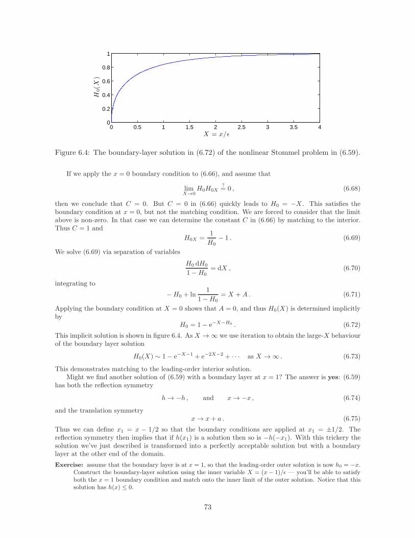
0 0.5 1 1.5 2 2.5 3 3.5 40

0.2

0.4

0.6

0.8

1

X = x/ǫ

H0(X

)

Figure 6.4: The boundary-layer solution in (6.72) of the nonlinear Stommel problem in (6.59).

If we apply the x = 0 boundary condition to (6.66), and assume that

limX→0

H0H0X?= 0 , (6.68)

then we conclude that C = 0. But C = 0 in (6.66) quickly leads to H0 = −X . This satisfies theboundary condition at x = 0, but not the matching condition. We are forced to consider that the limitabove is non-zero. In that case we can determine the constant C in (6.66) by matching to the interior.Thus C = 1 and

H0X =1

H0− 1 . (6.69)

We solve (6.69) via separation of variables

H0 dH0

1−H0= dX , (6.70)

integrating to

−H0 + ln1

1−H0= X +A . (6.71)

Applying the boundary condition at X = 0 shows that A = 0, and thus H0(X) is determined implicitlyby

H0 = 1− e−X−H0 . (6.72)

This implicit solution is shown in figure 6.4. As X → ∞ we use iteration to obtain the large-X behaviourof the boundary layer solution

H0(X) ∼ 1− e−X−1 + e−2X−2 + · · · as X → ∞ . (6.73)

This demonstrates matching to the leading-order interior solution.Might we find another solution of (6.59) with a boundary layer at x = 1? The answer is yes: (6.59)

has both the reflection symmetry

h→ −h , and x→ −x , (6.74)

and the translation symmetryx→ x+ a . (6.75)

Thus we can define x1 = x − 1/2 so that the boundary conditions are applied at x1 = ±1/2. Thereflection symmetry then implies that if h(x1) is a solution then so is −h(−x1). With this trickery thesolution we’ve just described is transformed into a perfectly acceptable solution but with a boundarylayer at the other end of the domain.

Exercise: assume that the boundary layer is at x = 1, so that the leading-order outer solution is now h0 = −x.Construct the boundary-layer solution using the inner variable X = (x− 1)/ǫ — you’ll be able to satisfyboth the x = 1 boundary condition and match onto the inner limit of the outer solution. Notice that thissolution has h(x) ≤ 0.

73

Reformulation of the nonlinear diffusion model

As a solution of the dirt-pile model the second solution above makes no sense: dirt piles can’t havenegative height. And the physical intuition that put the boundary layer at x = 0 can’t be wrong simplybecause we use a more complicated model of diffusion. The problem is that the nonlinear diffusionequation in (6.59) should be

ǫ(12 |h|h

)

xx+ hx = −1 , h(0) = h(1) = 0 . (6.76)

In other words, the diffusivity should vary with |h|, not h. Back in (6.59), our translation of the physicalproblem into mathematics was faulty. Changing h to |h| in destroys the symmetry in (6.74).

Now let’s use the correct model in (6.76) and show that the boundary layer cannot be at x = 1. Ifwe try to put the boundary layer at x = 1 then the leading-order interior solution is

h0 = −x . (6.77)

Using the boundary layer coordinate

Xdef=

x− 1

ǫ, (6.78)

the leading-order boundary layer equation is

−(

12H

20

)

XX+H0X = 0 , (6.79)

Above we have assumed that H0(X) < 0 so that |H0| = −H0. The differential equation in (6.82) mustbe solved with boundary and matching conditions

H0(0) = 0 , and limX→−∞

H0 = −1 . (6.80)

The second condition above is matching onto the inner limit of the outer solution. We can integrate(6.82) and apply the matching condition to obtain

dH0

dX=H0 + 1

H0. (6.81)

Now if −1 < H0 < 0 then the equation above implies that

dH0

dX< 0 . (6.82)

The sign in (6.82) is not consistent with a solution that increases monotonically from H0(−∞) = −1 toH0(0) = 1. Moreover if we integrate (6.81) with separation of variables we obtain an implicit solution

X = H0 − ln(1 +H0) , or equivalently H0 = −1 + e−X+H0 . (6.83)

But as X → −∞ we do not get a match — the boundary layer cannot be at x = 1. Thus we cannotconstruct a solution of the |h|-model in (6.76) with a boundary layer at x = 1

74

0 0.1 0.2 0.3 0.4 0.5 0.6 0.7 0.8 0.9 10

0.5

1

x

h(x

)

ǫ = 0.05ǫ = 0.05

Figure 6.5: Figure for problem 6.3.

6.5 Problems

Problem 6.1. (i) Find a leading order uniformly valid solution of

−hx = ǫhxx + x , h(0) = h(1) = 0 .

(ii) Solve the BVP above exactly and compare the exact solution to the boundary layer approximationwith ǫ = 0.1.

Problem 6.2. (i) Solve the boundary value problem

hx = ǫhxx + sinx , h(0) = h(π) = 0 ,

exactly. To assist communication, please use the notation

Xdef=

x− π

ǫ, and E

def= e−π/ǫ .

This should enable you to write the exact solution in a compact form. (ii) Find the first three terms inthe regular perturbation expansion of the outer solution

h(x) = h0(x) + ǫh1(x) + ǫ2h2(x) +O(ǫ3).

(iii) There is a boundary layer at x = π. “Rescale” the equation using X above as the independentvariable and denote the solution in the boundary layer by H(X). Find the first three terms in the regularperturbation expansion of the boundary-layer equation:

H = H0(X) + ǫH1(X) + ǫ2H2(X) +O(ǫ3).

(iv) The Hn’s above will each contain an unknown constant. Determine the three constants by matchingto the interior solution. (v) Construct a uniformly valid solution, up to an including terms of order ǫ2.You can check your algebra by comparing your boundary layer solution with the expansion of the exactsolution from part (i). (vi) With ǫ = 0.2 and 0.5, use matlab to compare the exact solution from part(i) with the approximation in part (v).

Problem 6.3. Find a leading-order boundary layer solution to the forced Burgers equation

ǫhxx +(12h

2)

x= −1 , h(0) = h(1) = 0 .

Use bvp4c to solve this problem numerically, and compare your leading order solution to the numericalsolution: see figure 6.5.

75

Problem 6.4. The result of problem 6.3 is disappointing: even though ǫ = 0.05 seems rather small, theapproximation in Figure 6.5 is only so-so. Calculate the next correction and compare the new improvedsolution with the bvp4c solution. (The numerical solution seems to have finite slope at x = 1, while theleading-order outer solution has infinite slope as x→ 1: perhaps there a higher-order boundary layer atx = 1 is required to heal this singularity?)

Problem 6.5. Use boundary layer theory to find leading order solution of

hx = ǫ(13h

3)

xx+ 1 , (6.84)

on the domain 0 < x < 1 with boundary conditions h(0) = h(1) = 0. You can check your answer byshowing that h = 1/2 at x ≈ 1− 0.057ǫ.

76

Lecture 7

More boundary layer theory

7.1 Variable speed

Suppose the conveyor belt is a stretchy membrane which moves with non-uniform speed −c(x). Withnon-constant c, the dirt conservation equation in (6.1) generalizes to

ht − (ch)x = s+ κhxx , (7.1)

with boundary conditions unchanged: h(0, t) = 0 and h(ℓ, t) = 0.

Exercise: Make sure you understand why it is (ch)x, rather than chx, in (7.1). Nondimensionalize (7.1) so thatthe steady state problem is

ǫhxx − (ch)x = −s , h(0) = h(1) = 0 , (7.2)

with max c(x) = 1 and max s(x)=1.

Example: A slow down

Suppose that the belt slows near x = 0. Specifically, let’s assume that the belt speed is

c =√x . (7.3)

The speed is zero at x = 0, so we expect that dirt will start to pile up. If the source is uniform then thesteady-state problem is

ǫhxx +(√xh)

x= −1 , with BCs h(0) = h(1) = 0. (7.4)

Exercise: Show that a particle starting at x = 1 and moving with x = −xβ, with β < 1, reaches x = 0 in afinite time. What happens if β ≥ 1?

The first two terms in the interior solution are

h(x, ǫ) =(

x−1/2 − x1/2)

+ ǫ

(1

2x−2 +

1

2x−1 − x−1/2

)

+ ord(ǫ2) . (7.5)

We’ve satisfied the BC at x = 1 and the pile-up at x = 0 is evident via the divergence of the outersolution as x → 0. Notice that this divergence is stronger at higher orders, and the RPS above isdisordered as x→ 0.

Turning to the boundary layer at x = 0, we introduce

Xdef=

x

δ(7.6)

so thatǫ

δ2hXX +

1

δ1/2

(√Xh)

X= −1 . (7.7)

77

A dominant balance between the first two terms is achieved with ǫ = δ3/2, or

δ = ǫ2/3 . (7.8)

With this definition of δ, andh = H(X, ǫ) , (7.9)

the boundary layer equation is

HXX +(√

XH)

X= −ǫ1/3 . (7.10)

We attack with an RPS: h = H0(X) + ǫ1/3H1(x) + · · ·At leading order

H0XX +(√

XH0

)

X= 0 , (7.11)

with first integralH0X +

√XH0 = A0 . (7.12)

Solving this first-order equation with an integrating factor we obtain

H0(X) = A0e−2X3/2/3

∫ X

0

e2t3/2/3 dt . (7.13)

We’ve satisfied the boundary condition at x = 0, and we must determine the remaining constant ofintegration A0 by matching to the interior solution.

To match the interior, we need the asymptotic expansion of (7.13) as X → ∞: this can be obtainedby following our earlier discussion of Dawson’s integral:

H0(X) ∼ A0√X, as X → ∞, (7.14)

=ǫ1/3A0

x1/2. (7.15)

An alternative, and more efficient, derivation of (7.15) is to write (7.12) as

H0 =A0

X1/2− H0X

X1/2(7.16)

and proceed iteratively starting with H0 ∼ A0X−1/2 as X → ∞.

On the other hand the inner expansion of the outer solution in (7.5) is

h =1

x1/2+O

(

x1/2, ǫx−2)

. (7.17)

We almost have a match — it seems we should take A0 = ǫ−1/3 in (7.15) so that both functions areequal to x−1/2 in the matching region. But remember that we assumed that H0(x) is independent of ǫ,so A0 cannot depend on ǫ. Our expansion has failed.

Exercise: How would you gear so that the term ǫx−2 in (7.15) is asymptotically negligible relative to x−1/2 inthe matching region?

Fortunately there is a simple cure: the correct definition of the boundary layer solution — whichreplaces (7.9) — is

h = ǫ−1/3H(X, ǫ) . (7.18)

In retrospect perhaps the rescaling in (7.18) is obvious — the interior RPS in (7.5) is becoming disorderedas x → 0. The problem is acute once the second term in the expansion is comparable to the first term,which happens once

x−1/2 ∼ ǫx−2 or x ∼ ǫ2/3 = δ . (7.19)

78

0 0.2 0.4 0.6 0.8 10

0.5

1

1.5

x

h(x

)

ǫ = 0.05

O (ǫ) unifexact

Figure 7.1: Comparison of (7.23) with the exact solution of (7.4).

This the boundary layer scale, and as we enter this region the interior solution is of order x−1/2 ∼ ǫ−1/3

— this is why the rescaling in (7.18) is required. If we’d been smart we would have made this argumentimmediately after (7.5) and avoided the mis-steps in (7.9) and (7.10).

Using the rescaled variable in (7.15), the boundary layer equation that replaces (7.10) is

HXX +(√

XH)

X= −ǫ2/3 . (7.20)

Now we can try the RPSH(X, ǫ) = H0(X) + ǫ2/3H1(X) + · · · (7.21)

We quickly find the leading order solution

H0 = e−2X3/2/3

∫ X

0

e2t3/2/3 dt . (7.22)

This satisfies the x = 0 boundary condition and also matches the x−1/2 from the interior.We can now construct a leading-order uniformly valid solution as

huni(x, ǫ) = ǫ−1/3e−2X3/2/3

∫ X

0

e2t3/2/3 dt− x1/2 . (7.23)

Figure 7.1 compares the uniformly valid approximation (7.23) with an exact solution of (7.4).

Exercise: evaluate the integral∫ 1

0h(x, ǫ) dx to leading order as ǫ → 0.

Example: higher-order corrections

To illustrate how to bash out higher order corrections let’s calculate the first two terms in the BL solutionof the BVP

ǫhxx + [exh]x = −2e2x , with BCs h(0) = h(1) = 0 . (7.24)

We suspect there is a BL at x = 0. So we first develop the interior solution

h(x, ǫ) = h0(x) + ǫh1(x) + ǫh2(x) + · · · (7.25)

by satisfying the boundary condition at x = 1 at every order.The leading-order term is

[exh0]x = −2e2x , ⇒ h0 = e2−x − ex . (7.26)

The next two orders are

[exh1]x = −h0xx , ⇒ h1 = 1− 2e1−x + e2−2x , (7.27)

[exh2]x = −h1xx , ⇒ h2 = 2(e2−3x − e1−2x

). (7.28)

79

Later, to perform the match, we will need the inner limit of this outer solution. So in preparation forthat, as x→ 0,

h0 + ǫh1 + ǫ2h2 = (e2 − 1)− (e2 + 1)x+ 12 (e

2 − 1)x2

+ ǫ(1− e)2 − ǫx2(e2 − e)

+ ǫ22(e2 − e) + ord(x3, ǫx2, ǫ2x) . (7.29)

Turning to the boundary layer, we use the inner variable X = x/ǫ so that the rescaled differentialequation is

hXX +[eǫXh

]

X= −2ǫe2ǫX . (7.30)

We substitute the inner expansion

h = H0(X) + ǫH1(X) + ǫ2H2(X) + · · · (7.31)

into the differential equation and collect powers of ǫ. The first three orders of the boundary-layer problemare

H0XX +H0X = 0 , (7.32)

H1XX + [H1 +XH0]X = −2 , (7.33)

H2XX +[H2 +XH1 +

12X

2H0

]

X= −4X . (7.34)

Note that it is necessary to expand the exponentials within the boundary layer, otherwise we cannotensure that the Hn’s do not depend on ǫ.

The solution for H0 that satisfies the boundary condition at x = 0, and also matches the first termon the right of (7.29), is

H0 = (e2 − 1)(1− e−X

). (7.35)

The solution for H1 that satisfies the boundary condition at x = 0 is

H1 = A1(1 − e−X) + (e2 + 1)(1−X − e−X

)+ 1

2 (e2 − 1)X2e−X . (7.36)

The constant A1 is determined by matching to the interior solution. We can do this by taking the limitas X → ∞ in the boundary layer solution H0 + ǫH1. Effectively this means that all terms involvinge−X are exponentially small and therefore negligible in the matching. To help with pattern recognitionwe rewrite the outer limit of the boundary-layer solution in terms of the outer variable x. Thus, in thematching region where X ≫ 1 and x≪ 1, the boundary-layer solution in (7.35) and (7.36) is:

H0 + ǫH1 → (e2 − 1) + ǫA1 + ǫ(1 + e2)− (1 + e2)x . (7.37)

To match the first term on the second line of (7.29) with (7.37) we require

ǫA1 + ǫ(1 + e2) = ǫ(1− e)2 , ⇒ A1 = −2e . (7.38)

The final term in (7.37), namely −(1 + e2)x, matches against a term on the first line of (7.29). That’sinteresting, because −(1 + e2)x comes from H1 and matches against h0.

There are many remaining ummatched terms in (7.29) e..g, 12 (e

2 − 1)x2 on the first line. This termwill match against terms from H2 i.e., it will require an infinite number of terms in the boundary layerexpansion just to match terms arising from the expansion of the leading-order interior solution.

Now we construct a uniformly valid approximation using the recipe

uniform = outer + inner−match . (7.39)

This gives

huni = e2−x − ex − (e2 − 1)e−X

+ ǫ[1− 2e1−x + e2−2x + e−X

(12X

2(e2 − 1)− (e− 1)2)]. (7.40)

This construction satisfies the x = 0 boundary condition exactly. But there is an exponentially smallembarrassment at x = 1. Figure 7.2 compares the numerical solution of (7.24) with the approximationin (7.40). At ǫ = 0.2 the two-term approximation is significantly better than just the leading-order term.We don’t get line-width agreement — the ǫ2 term would help.

80

0 0.1 0.2 0.3 0.4 0.5 0.6 0.7 0.8 0.9 10

1

2

3

x

h

ǫ = 0.2ǫ = 0.2 bvp4c

two termsone term

Figure 7.2: Comparison of the one and two term uniform approximations in (7.40) with thenumerical solution of (7.24).

81

function StommelBL

% Solution of epsilon h_xx +(exp(x) h)_x = - 2 \exp(2 x)

epsilon = 0.2;

solinit = bvpinit(linspace(0 , 1 , 10) , @guess);

sol = bvp4c(@odez,@bcs,solinit);

% My fine mesh

xx = linspace(0,1,100); hh = deval(sol,xx);

figure; subplot(2,1,1)

plot(xx , hh(1,:),’k’)

hold on

xlabel(’$x$’,’interpreter’,’latex’,’fontsize’,16)

ylabel(’$h$’,’interpreter’,’latex’,’fontsize’,16,’rotation’,0)

axis([0 1 0 3.5])

% The BL solution

XX = xx/epsilon; EE =exp(-XX);

hZero = exp(2-xx) - exp(xx) - (exp(2) - 1).*EE;

hOne = 1 - 2*exp(1-xx) + exp(2-2*xx)...

+ EE.*( 0.5*XX.^2*(exp(2) - 1) - (exp(1) - 1)^2);

plot(xx, hZero+epsilon*hOne,’-.r’ , xx,hZero,’--g’)

legend(’bvp4c’,’two terms’ , ’one term’)

text(0.02,3.2,’$\epsilon =0.2$’,’interpreter’,’latex’,’fontsize’,16)

%% Inline functions

%The differential equations

function dhdx = odez(x,h)

dhdx = [h(2)/epsilon ; ...

- exp(x).*h(2)/epsilon - exp(x).*h(1) - 2*exp(2*x)];

end

%residual in the boundary condition

function res = bcs(um,up)

res = [um(1) ; up(1) ];

end

% Inital guess at the solution

function hinit = guess(x)

hinit = [(1-x^2) ; 2*x];

end

end

82

7.2 A second-order BVP with a boundary layer

At the risk of repetition, let’s discuss another elementary example of boundary layer theory, focussingon intuitive concepts and on finding the leading-order uniformly valid solution. We use the BVP

ǫy′′ + a(x)y′ + b(x)y = 0 , (7.41)

with BCsy(0) = p , y(1) = q , (7.42)

as our model.

The case a(x) > 0

In the outer region we can look for a solution with the expansion

y(x, ǫ) = y0(x) + ǫy1(x) + · · · (7.43)

The leading-order term satisfiesay′0 + by0 = 0 . (7.44)

Solutions of this first order differential equation cannot satisfy two boundary conditions. With theconstruction

y0(x) = q exp

(∫ 1

x

b(v)

a(v)dv

)

(7.45)

we have satisfied the boundary condition at x = 1. We return later to discuss why this is the correctchoice if a(x) > 0. (If a(x) < 0 the boundary layer is at x = 1 and the outer solution should satisfy theboundary condition at x = 0.)

Unless we’re very lucky, (7.45) will not satisfy the boundary condition at x = 0. Let’s try to fix thisproblem by building a boundary layer at x = 0. Begin by introducing a boundary layer coordinate

Xdef=

x

ǫ, (7.46)

and writingy(x, ǫ) = Y (X, ǫ) . (7.47)

Then “re-scale” the differential equation (7.41) using the boundary-layer variables:

YXX + a(ǫX)YX + ǫb(ǫX)Y = 0 . (7.48)

Notice that within the boundary layer, where X = ord(1),

a(ǫX) = a(0) + ǫXa′(0) + 12ǫ

2X2a′′(0) + ord(ǫ3). (7.49)

There is an analogous expansion for b(ǫX).In the boundary layer we use the “inner expansion”:

Y (X, ǫ) = Y0(X) + ǫY1(X) + · · · (7.50)

The leading-order term isǫ0 : Y0XX + a(0)Y0X = 0 , (7.51)

and, for good measure, the next term is

ǫ1 : Y1XX + a(0)Y1X + a′(0)XY0X + b(0)Y0 = 0 . (7.52)

Terms in the Taylor series (7.49) will impact the higher orders.

83

The solution of (7.51) that satisfies the boundary condition at X = 0 is

Y0 = p+A0

(

1− e−a(0)X)

, (7.53)

where A0 is a constant of integration. We are assuming that a(0) > 0 so that the exponential in (7.53)decays to zero as X → ∞. This is why the boundary layer must be at x = 0. The constant A0 can thenbe determined by demanding that in the outer solution (7.45) agrees with the inner solution (7.53) inthe matching region where X ≫ 1 and x≪ 1. This requirement determines A0:

p+A0 = q exp

(∫ 1

0

b(v)

a(v)dv

)

. (7.54)

Hence the leading order boundary-layer solution is

Y0 = p+

[

q exp

(∫ 1

0

b(v)

a(v)dv

)

− p

] (

1− e−a(0)X)

, (7.55)

= pe−a(0)X + q exp

(∫ 1

0

b(v)

a(v)dv

)(

1− e−a(0)X)

. (7.56)

We construct a uniformly valid solutions using the earlier recipe

uniformly valid = outer + inner−match . (7.57)

In this case we obtain

yuni = q exp

(∫ 1

x

b(v)

a(v)dv

)

+

[

p− q exp

(∫ 1

0

b(v)

a(v)dv

)]

e−a(0)X . (7.58)

7.3 Other BL examples

Not all boundary layers have thickness ǫ. Let’s quickly consider some examples.

Example:

ǫy′′ − y = −f(x) , y(−1) = y(1) = 0 , (7.59)

If we solve the simple case with f(x) = 1 exactly we quickly see that y ≈ 1, except that there are boundarylayers with thickness

√ǫ at both x = 0 and x = 1.

Thus we might hope to construct the outer solution of (7.59) via the RPS

y = f + ǫf ′′ + ǫ2f′′′′

+ ord(ǫ3) . (7.60)

The outer solution above doesn’t satisfy either boundary condition: we need boundary layers at x = −1,and at x = +1.

Turning to the boundary layer at x = −1 we introduce

Xdef=

x+ 1√ǫ, and y(x, ǫ) = Y (X,

√ǫ) . (7.61)

The re-scaled differential equation is

YXX − Y = f(−1 +

√ǫX), (7.62)

and we look for a solution with

Y = Y0(X) +√ǫY1(X) + ǫY2(X) + · · · (7.63)

The leading-order problem isY0XX − Y0 = −f(−1) , (7.64)

with solutionY0 = f(−1) + A0e

−X + B0︸︷︷︸

=0

eX . (7.65)

84

We quickly set the constant of integration B0 to zero — the alternative would prevent matching with theinterior solution. Then the other constant of integration A0 is determined so that the boundary conditionat X = 0 is satisfied:

Y0 = f(−1)(

1− e−X)

. (7.66)

The boundary condition at x = +1 is satisfied with an analogous construction using the coordinate

Xdef= (x− 1)/

√ǫ. One finds

Y0 = f(1)(

1− eX)

. (7.67)

Notice that the outer limit of this boundary layer is obtained by taking X → −∞.

Finally we can construct a uniformly valid solutions via

yuni(x) = f(x)− f(−1)e−(x+1)/√

ǫ − f(+1)e(x−1)/√

ǫ . (7.68)

Example:

ǫy′′ + y = f(x) , y(0) = y(1) = 0 , (7.69)

If we solve the simple case with f(x) = 1 exactly we quickly see that this is not a boundary layer problem.This belongs in the WKB lecture.

Example: Find the leading order BL approximation to

ǫu′′ − u = − 1√1− x2

, with BCs u(±1) = 0 . (7.70)

The leading-order outer solution is

u0 =1√

1− x2. (7.71)

Obviously this singular solution doesn’t satisfy the boundary conditions. We suspect that there areboundary layers of thickness

√ǫ at x = ±1. Notice that the interior solution (7.71) is ∼ ǫ−1/4 as x moves

into this BL. Moreover, considering the BL at x = −1, we use X = (1 + x)/√ǫ as the boundary layer

coordinate, so that1√

1− x2=

1

ǫ1/4√

X(2−√ǫX)

. (7.72)

Hence we try a boundary-layer expansion with the form

u(x, ǫ) = ǫ−1/4[U0(X) +

√ǫU1(X) + ord(ǫ)

]. (7.73)

A main point of this example is that it is necessary to include the factor ǫ−1/4 above.

The leading-order term in the boundary layer expansion is then

U ′′0 − U0 = − 1√

X, (7.74)

which we solve using variation of parameters

U0(X) = 12e−X

∫ X

0

ev√vdv

︸ ︷︷ ︸

∼eX/√

X

− 12eX∫ X

0

e−v

√vdv

︸ ︷︷ ︸

∼√π−(e−X/

√X)

+P eX +Qe−X . (7.75)

The boundary condition at X = 0 requires

P +Q = 0 . (7.76)

To match the outer solution as X → ∞, we must use the X → ∞ asymptotic expansion of the integralsin (7.75), indicated via the underbrace. We determine P so that the exponentially growing terms areeliminated, which requires that P =

√π/2. Thus the boundary layer solution is

U0(X) =√π sinhX −

∫ X

0

sinh(X − v)√v

dv . (7.77)

(Must check this, and then construct the uniformly valid solution!)

85

Example: Find the leading order BL approximation to

ǫy′′ + xy′ + x2y = 0 , with BCs y(0) = p , y(1) = q . (7.78)

We divide and conquer by writing the solutions as

y = pf(x, ǫ) + qg(x, ǫ) , (7.79)

whereǫf ′′ + xf ′ + x2f = 0 , with BCs f(0) = 1 , f(1) = 0 , (7.80)

andǫg′′ + xg′ + x2g = 0 , with BCs g(0) = 0 , g(1) = 1 , (7.81)

The outer solution of the g-problem is

g = e(1−x2)/2 + ǫg1 + · · · (7.82)

We need a BL at x = 0. A dominant balance argument shows that the correct BL variable is

X =x√ǫ, (7.83)

and if g(x, ǫ) = G(X,√ǫ) then the rescaled problem is

GXX +XGX + ǫX2G = 0 . (7.84)

The leading-order problem isG0XX +XG0X = 0 , (7.85)

with general solution

G0 = P︸︷︷︸

=0

+ Q︸︷︷︸√e/2π

∫ X

0

e−v2/2 dv . (7.86)

To satisfy the X = 0 boundary condition we take P = 0, and to match the outer solution we require

Q

∫ ∞

0

e−v2/2 dv =√e . (7.87)

The uniformly valid solution is

guni(x, ǫ) = e(1−x2)/2 +

√e

2π

∫ x/√ǫ

0

e−v2/2 dv −√e , (7.88)

= e(1−x2)/2 −√

e

2π

∫ ∞

x/√ǫ

e−v2/2 dv . (7.89)

Now turn to the f -problem. The outer solution is fn(x) = 0 at all orders. The solution of the leading-orderboundary-layer problem is

F0(X) =1√2π

∫ ∞

X

e−v2/2 dv . (7.90)

This is a stand-alone boundary layer.

Example: Let’s analyze the higher-order terms in the BL solution of our earlier example

ǫy′′ − y = −f(x) , y(−1) = y(1) = 0 . (7.91)

Our provisional outer solution is

y(x) = f(x) + ǫf ′′(x) + ǫ2f ′′′′(x) + ord(ǫ3) . (7.92)

Let’s rewrite this outer solution in terms of the inner variable Xdef= (x− 1)/

√ǫ

y(x) = f(1 +√ǫX) + ǫf ′′(1 +

√ǫX) + ǫ2f ′′′′(1 +

√ǫX) + ord(ǫ3) . (7.93)

86

Assuming that√ǫX is small in the matching region, we expand the outer solution:

y(x) = f(1) +√ǫXf ′(1) + ǫ

(12X2 + 1

)f ′′(1) + ǫ3/2

(

X +1

6X3

)

f ′′′(1)

+ ǫ2(

1 +1

2X2 +

1

24X4

)

f ′′′′(1) + ord(

ǫ5/2)

. (7.94)

We hope that the outer expansion of the inner solution at x = 1 will match the series above.

The rescaled inner problem is

YXX − Y = −f(1 +√ǫX) , (7.95)

= −f(1)−√ǫXf ′(1)− ǫ

1

2X2f ′′(1) + ord(ǫ3/2) . (7.96)

The RPS isY = f(1)

(

1− eX)

+√ǫY1(X) + ǫY2(X) + ǫ3/2Y3(X)ord(ǫ2) , (7.97)

with

Y ′′1 − Y1 = −Xf ′(1) , (7.98)

Y ′′2 − Y2 = − 1

2X2f ′′(1) , (7.99)

Y ′′3 − Y3 = −1

6X3f ′′′(1) . (7.100)

We solve the equations above, applying the boundary condition Yn(0) = 0, to obtain

Y1(X) = Xf ′(1) , Y2(X) =(

1 + 12X2 − eX

)

f ′′(1) , (7.101)

and Y3(X) =

(

X +1

6X3

)

f ′′′(1) . (7.102)

Notice how the inner limit of the leading-order outer solution, y0(x) = f(x), produces terms at all ordersin the matching region. In order to match all of y0(x) one requires all the Yn(X)’s.

7.4 Problems

Problem 7.1. Find the leading-order uniformly valid boundary-layer solution to the Stommel problem

− (exg)x = ǫgxx + 1 , with BCs g(0) = g(1) = 0 . (7.103)

Do the same for(exf)x = ǫfxx + 1 , with BCs f(0) = f(1) = 0 . (7.104)

Problem 7.2. Analyze the variable-speed Stommel problem

ǫh′′ + (xah)x = −1 , with BCs h(0) = h(1) = 0 , (7.105)

using boundary layer theory. (The case a = 1/2 was discussed in the lecture.) How thick is the boundarylayer at x = 0, and how large is the solution in the boundary layer? Check your reasoning by constructingthe leading-order uniformly valid solution when a = −1, a = 1 and a = 2.

Problem 7.3. Find the leading-order, uniformly valid solution of

ǫh′′ + (sinxh)x = −1 , with BCs h(0) = h(π

2

)

= 0 . (7.106)

Problem 7.4. Find a leading-order boundary layer solution to

ǫh′′ + (sinxh)x = −1, with BCs h(0) = h(π) = 0 . (7.107)

(I think there are boundary layers at both x = 0 and x = 1.)

87

Problem 7.5. Considering the slow-down example (7.4), find the next term in the boundary-layersolution of this problem. Make sure you explain how the term ǫx−2 in the outer expansion is matchedas x→ 0.

Problem 7.6. Assuming that a(x) < 0, construct the uniformly valid leading-order approximation tothe solution of

ǫy′′ + ay′ + by = 0 , with BCs y′(0) = p , y′(1) = q . (7.108)

(Consider using linear superposition by first taking (p, q) = (1, 0), and then (p, q) = (0, 1).)

Problem 7.7. Consider

ǫy′′ +√xy′ + y = 0 , with BCs y(0) = p , y(1) = q . (7.109)

(i) Find the rescaling for the boundary layer near x = 0, and obtain the leading order inner approx-imation. Then find the leading-order outer approximation and match to determine all constants ofintegration. (ii) Repeat for

ǫy′′ −√xy′ + y = 0 , with BCs y(0) = p , y(1) = q . (7.110)

Problem 7.8. Find a leading order, uniformly valid solution of

ǫy′′ +√xy′ + y2 = 0 , (7.111)

posed on 0 < x < 1 with boundary conditions y(0; ǫ) = 2 and y(1; ǫ) = 1/3.

Problem 7.9. Find a leading order, uniformly valid solution of

ǫy′′ − (1 + 3x2)y = x , with BCs y(0, ǫ) = y(1; ǫ) = 1 . (7.112)

Problem 7.10. Find a leading-order, uniformly valid solution of

ǫy′′ − y′

1 + 2x− 1

y= 0 , with BCs y(0, ǫ) = y(1; ǫ) = 3 . (7.113)

Problem 7.11. In an earlier problem you were asked to construct a leading order, uniformly validsolution of

ǫy′′ − (1 + 3x2)y = x , with BCs y(0, ǫ) = y(1; ǫ) = 1 . (7.114)

Now construct the uniformly valid two-term boundary layer approximation.

Problem 7.12. Consider

ǫy′′ + (1 + ǫ)y′ + y = 0 , y(0) = 0 , y(1) = e−1 , (7.115)

m′ = y , m(1) = 0 . (7.116)

Find two terms in the outer expansion of y(x) and m(x), applying only boundary conditions at x = 1.Next find two terms in the inner approximation at x = 0, applying the boundary condition at x = 0.Determine the constants of integration by matching. Calculate m(0) correct to order ǫ.

88

Lecture 8

Multiple scale theory

8.1 Introduction to two-timing

Begin by considering the damped harmonic oscillator

d2x

dt2+ β

dx

dt+ x = 0 , (8.1)

with initial conditions

x(0) = 0 , anddx

dt(0) = 1 . (8.2)

You should recall that the exact solution is

x = ν−1e−βt/2 sin νt , with νdef=

√

1− β2

4. (8.3)

A good or useful β ≪ 1 approximation to this exact solution is

x ≈ e−βt/2 sin t . (8.4)

Let’s use this example to motivate the multiple-scale method.

Failure of the regular perturbation expansion

If β ≪ 1 we might be tempted to try an RPS on (8.1):

x(t, β) = x0(t) + βx1(t) + β2x2(t) + · · · (8.5)

A reasonable goal is to produce the good approximation (8.4). The RPS will not be successful and thisfailure will drive us towards the method of multiple time a scales, also know as “two timing”.

The leading-order problem is

x0 + x0 = 0 , with IC x0 = 0 , x0(0) = 1 . (8.6)

The solution isx0 = sin t . (8.7)

The first-order problem is

d2x1dt2

+ x1 = − cos t , with IC x1(0) = 0 ,dx1dt

(0) = 0 . (8.8)

This is a resonantly forced oscillator equation, with solution

x1 = − t

2sin t . (8.9)

89

0 5 10 15 20 25 30 35 40−1

−0.5

0

0.5

1

t

x(t)

β = 0.2

Figure 8.1: Comparison of the exact solution in (8.3) (the solid black curve), with the two-term RPSin (8.10) (the blue dotted curve) and the two-time approximation in (??) (the dashed red curve). It isdifficult to distinguish the two-time approximation from the exact result.

Thus the developing RPS is

x(t, β) = sin t− βt

2sin t+ β2x2(t) + · · · (8.10)

At this point we recognize that the RPS is misleading: the exact solution damps to zero on a time scale2/β, while the RPS suggests that the solution is growing linearly with time. With hindsight we realizethat the RPS is producing the Taylor series expansion of the exact solution in (8.3) about β = 0. Usingmathematica, this series is

x(t, β) = sin t− βt

2sin t+

β2

8

[t2 sin t+ sin t− t cos t

]+O(β3) . (8.11)

Calculating more terms in the RPS will not move us closer to the useful approximation in (8.4): insteadwe’ll grind out the useless approximation in (8.11). In this example the small term in (8.1) is smallrelative to the other terms at all times. Yet the small error slowly accumulates over long times ∼ β−1.This is a secular error.

Two-timing

Looking at the good approximation in (8.4) we are inspired to introduce a slow time:

sdef= βt . (8.12)

We assume that x(t, β) has a perturbation expansion of the form

x(t, β) = x0(t, s) + βx1(t, s) + β2x3(t, s) + · · · (8.13)

Notice how this differs from the RPS in (8.5).At each order xn is a function of both s and t a function of both t and s. To keep track of all the

terms we use the ruled

dt= ∂t + β∂s , (8.14)

and the equation of motion is

(∂t + β∂s)2x+ β (∂t + β∂s)x+ x = 0 . (8.15)

At leading order

β0 : ∂2t x0 + x0 = 0 , with general solution x0 = A(s)eit +A∗(s)e−it . (8.16)

90

Notice that the “constant of integration” is actually a function of the slow time s. We determine theevolution of this function A(s) at next order1.

At next order

β1 : ∂2t x1 + x1 = −2x0ts − x0t , (8.18)

= −2iAseit − iAeit + c.c. (8.19)

Again we have a resonantly forced oscillator. but this time we can prevent the secular growth of x1 onthe fast time scale by requiring that

2As +A = 0 . (8.20)

Thus the leading-order solution is

x0(s, t) = A0e−s/2eit +A∗

0e−s/2e−it . (8.21)

The constant of integration A0 is determined to satisfy the initial conditions. This requires

0 = A0 +A∗0 , 1 = iA0 − iA∗

0 , ⇒ A0 = 12 i . (8.22)

Thus we have obtained the good approximation

x0 = e−βt/2 sin t . (8.23)

Averaging

8.2 The Duffing oscillator

We consider an oscillator with a nonlinear spring

mx+ k1x+ k3x3 = 0 , (8.24)

and an initial conditionx(0) = x0 x(0) = 0 . (8.25)

If k3 > 0 then the restoring force is stronger than linear — this is a stiff spring.We can non-dimensionalize this problem into the form

x+ x+ ǫx3 = 0 , (8.26)

with the initial conditionx(0) = 1 x(0) = 0 . (8.27)

We use this Duffing oscillator as an introductory example of the multiple time scale method.Energy conservation,

12 x

2 + 12x

2 + 14ǫx

4 = E︸︷︷︸

=12+

14 ǫ

, (8.28)

immediately provides a phase-plane visualization of the solution and shows that the oscillations arebounded.

Exercise: Show that in (8.26), ǫ = k3x20/k1.

Exercise: Derive (8.28).

1We could alternatively write the general solution of the leading order problem as

x0 = R cos(t+ φ) , (8.17)

where the amplitude R and the phase φ are as yet undetermined functions of s. I think the complex notation in(8.16) is a little simpler.

91

The naive RPSx = x0(t) + ǫx1(t) + · · · (8.29)

leads tox0 + x0 = 0 , ⇒ x0 = cos t , (8.30)

and at next order

x1 + x1 = − cos3 t , (8.31)

= − 18

(e3it + 3eit + c.c.

), (8.32)

= − 14 cos 3t− 3

4 cos t . (8.33)

The x1-oscillator problem is resonantly forced and the solution will grow secularly, with x1 ∝ t sin t.Thus the RPS fails once t ∼ ǫ−1.

Two-timing

Instead of an RPS we use the two-time expansion

x = x0(s, t) + ǫx1(s, t) + · · · (8.34)

where s = ǫt is the slow time. Thus the expanded version of (8.26) is

(∂t + ǫ∂s)2(x0(s, t) + ǫx1(s, t) + · · · ) + (x0(s, t) + ǫx1(s, t) + · · · )

+ ǫ (x0(s, t) + ǫx1(s, t) + · · · )3 = 0 (8.35)

The leading order is∂2t x0 + x0 = 0 , (8.36)

with general solutionx0 = A(s)eit +A∗(s)e−it . (8.37)

The amplitude A is a function of the slow time s. At next order, ǫ1, we have

∂2t x1 + x1 = −2∂t∂sx0 − x30 , (8.38)

= −2iAseit −A3e3it − 3A2A∗eit + c.c. (8.39)

To prevent the secular growth of x1 we must remove the resonant terms, e±it on the right of (8.39) —this prescription determines the evolution of the slow time:

2iAs + 3|A|2A = 0 . (8.40)

The remaining terms in (8.39) are

∂2t x1 + x1 = −A3e3it + c.c. (8.41)

The solution will be x1 ∝ e±3it and will remain bounded.

Polar coordinates

To solve (8.40) it is best to transform to polar coordinates

A = r(s)eiθ(s) and As = (rs + irθs) eiθ ; (8.42)

substituting into the amplitude equation (8.40)

rs = 0 , and θs =3

2r2 . (8.43)

92

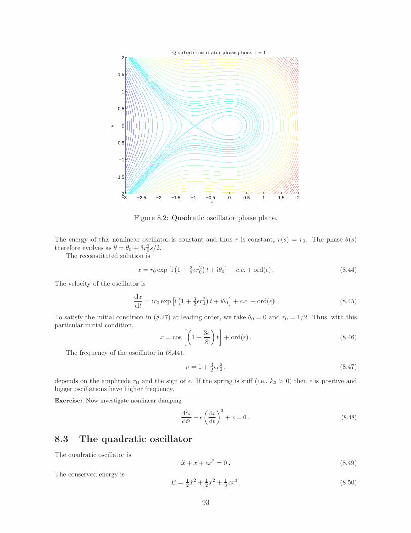
−3 −2.5 −2 −1.5 −1 −0.5 0 0.5 1 1.5 2−2

−1.5

−1

−0.5

0

0.5

1

1.5

2

x

u

Quadratic osci l lator phase plane, ǫ = 1

Figure 8.2: Quadratic oscillator phase plane.

The energy of this nonlinear oscillator is constant and thus r is constant, r(s) = r0. The phase θ(s)therefore evolves as θ = θ0 + 3r20s/2.

The reconstituted solution is

x = r0 exp[i(1 + 3

2ǫr20

)t+ iθ0

]+ c.c.+ ord(ǫ) . (8.44)

The velocity of the oscillator is

dx

dt= ir0 exp

[i(1 + 3

2ǫr20

)t+ iθ0

]+ c.c.+ ord(ǫ) . (8.45)

To satisfy the initial condition in (8.27) at leading order, we take θ0 = 0 and r0 = 1/2. Thus, with thisparticular initial condition,

x = cos

[(

1 +3ǫ

8

)

t

]

+ ord(ǫ) . (8.46)

The frequency of the oscillator in (8.44),

ν = 1 + 32ǫr

20 , (8.47)

depends on the amplitude r0 and the sign of ǫ. If the spring is stiff (i.e., k3 > 0) then ǫ is positive andbigger oscillations have higher frequency.

Exercise: Now investigate nonlinear damping

d2x

dt2+ ǫ

(dx

dt

)3

+ x = 0 . (8.48)

8.3 The quadratic oscillator

The quadratic oscillator isx+ x+ ǫx2 = 0 . (8.49)

The conserved energy isE = 1

2 x2 + 1

2x2 + 1

3ǫx3 , (8.50)

93

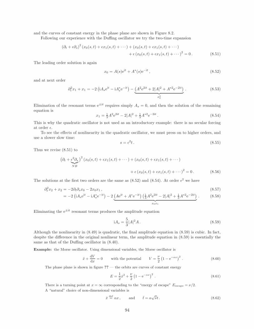
and the curves of constant energy in the phase plane are shown in Figure 8.2.Following our experience with the Duffing oscillator we try the two-time expansion

(∂t + ǫ∂s)2(x0(s, t) + ǫx1(s, t) + · · · ) + (x0(s, t) + ǫx1(s, t) + · · · )

+ ǫ (x0(s, t) + ǫx1(s, t) + · · · )2 = 0 . (8.51)

The leading order solution is again

x0 = A(s)eit +A∗(s)e−it , (8.52)

and at next order

∂2t x1 + x1 = −2(iAse

it − iA∗se

−it)−(A2e2it + 2|A|2 +A∗2e−2it

)

︸ ︷︷ ︸

x20

. (8.53)

Elimination of the resonant terms e±it requires simply As = 0, and then the solution of the remainingequation is

x1 = 13A

2e2it − 2|A|2 + 13A

∗2e−2it . (8.54)

This is why the quadratic oscillator is not used as an introductory example: there is no secular forcingat order ǫ.

To see the effects of nonlinearity in the quadratic oscillator, we must press on to higher orders, anduse a slower slow time:

s = ǫ2t . (8.55)

Thus we revise (8.51) to

(∂t + ǫ2∂s

︸︷︷︸

NB

)2(x0(s, t) + ǫx1(s, t) + · · · ) + (x0(s, t) + ǫx1(s, t) + · · · )

+ ǫ (x0(s, t) + ǫx1(s, t) + · · · )2 = 0 . (8.56)

The solutions at the first two orders are the same as (8.52) and (8.54). At order ǫ2 we have

∂2t x2 + x2 = −2∂t∂sx0 − 2x0x1 , (8.57)

= −2(iAse

it − iA∗se

−it)− 2

(Aeit +A∗e−it

) (13A

2e2it − 2|A|2 + 13A

∗2e−2it)

︸ ︷︷ ︸

x0x1

. (8.58)

Eliminating the e±it resonant terms produces the amplitude equation

iAs =5

3|A|2A . (8.59)

Although the nonlinearity in (8.49) is quadratic, the final amplitude equation in (8.59) is cubic. In fact,despite the difference in the original nonlinear term, the amplitude equation in (8.59) is essentially thesame as that of the Duffing oscillator in (8.40).

Example: the Morse oscillator. Using dimensional variables, the Morse oscillator is

x+dV

dx= 0 with the potential V =

ν

2

(1− e−αx)2 . (8.60)

The phase plane is shown in figure ?? — the orbits are curves of constant energy

E =1

2x2 +

ν

2

(1− e−αx

)2. (8.61)

There is a turning point at x = ∞ corresponding to the “energy of escape” Eescape = ν/2.

A “natural” choice of non-dimensional variables is

xdef= αx , and t = α

√νt . (8.62)

94

In these variables, ν → 1 and α → 1 in the barred equations. Thus, the non-dimensional equation ofmotion is

x+ e−x (1− e−x) = 0 . (8.63)

If we’re interested in small oscillations around the minimum of the potential at x = 0, then the smallparameter is supplied by an initial condition such as

x(0) = ǫ , and x(0) = 0 . (8.64)

We rescale withx = ǫX , (8.65)

so that the equation is

ǫX + e−ǫX(

1− e−ǫX)

= 0 , (8.66)

or

X +X − ǫ3

2X2 +

7

6ǫ2X3 = ord

(ǫ3). (8.67)

The multiple time scale expansion is now

X = X0(s, t) + ǫX1(s, t) + ǫ2X2(s, t) + · · · (8.68)

with slow time s = ǫ2t.

The main point of this example is that it is necessary to proceed to order ǫ2, and therefore to retain theterm 7ǫ2X3/6, to obtain the amplitude equation. One finds

iAs = (8.69)

8.4 Symmetry and universality of the Landau equation

So far the two-time expansion always leads to the Landau equation

As = pA+ q|A|2A . (8.70)

If you dutifully solve some of the early problems in this lecture you’ll obtain (8.70) again and again.Why is that? If we simply list all the terms up to cubic order that might occur in an amplitude equationwe have

As = ?A+?A∗+?A2+?|A|2+?A∗2+?A3 + ?|A|2A+?|A|2A∗+?A∗3 + · · · (8.71)

The coefficients are denoted by “?” and we’re not interested in the precise value of these numbers, exceptin so far as most of them turn out to be zero. The answer in (8.70) is simple because we have two termson the right, instead of the nine in (8.71). We’ve been down in the weeds calculating, but we have notasked the big question why do we have to calculate only the two coefficients p and q?

We have been considering only autonomous differential equations, such as

dx

dt+ x+ ǫx5 = 0 . (8.72)

This means that if x(t) is a solution of (8.72) then so is x(t − α), where α is any constant. In otherwords, the equations we’ve been considering are unchanged (“invariant”) if

t→ t+ α . (8.73)

Now if we try to solve (8.70) with a solution of the form

x(t) = A(s)eit +A∗(s)e−it + ǫx1(t, s) + · · · (8.74)

thenx(t + α) = Aeiα eit +A∗e−iα e−it + ǫx1 + · · · (8.75)

Thus the time-translation symmetry of the original differential equation implies that the amplitudeequation should be invariant under the rotation

A→ Aeiα , (8.76)

where α is any constant. Only the underlined terms in (8.71) respect this symmetry and therefore onlythe underlined terms can appear in the amplitude equation.

95

Exercise: many of our examples have time reversal symmetry i.e., the equation is invariant under t→ −t. Forexample, the nonlinear oscillator (with no damping) is invariant under t → −t. Show that this impliesthat p and q in (8.70) must be pure imaginary.

8.5 Parametric instability

Consider an oscillator whose frequency is changing slightly

d2x

dt2+(ω2 + ǫ cosσt

)x = 0 . (8.77)

How does the small fluctuation ǫ cosσt affect the oscillations?Let’s apply a multiple time scale approximation to (8.77). We’ll write the unperturbed (ǫ = 0)

solution asx = Aeiωt + c.c. (8.78)

When we switch on the perturbation the amplitude A becomes a function of slow time s = ǫt. Beforedoing the algebra, we show that the only terms in the amplitude equation (8.77) consistent with allsymmetries in (8.77) are

As =?A+?A∗ (8.79)

where ? indicates an imaginary constants.We attack with the multiple scale expansion

x = A(s)eiωt +A∗(s)e−iωt

︸ ︷︷ ︸

x0(s,t)

+ǫx1(s, t) + · · · (8.80)

where s = ǫt. At order ǫ1:

(∂2t + ω2

)x1 + 2iωAse

iωt − 2iωA∗se

−iωt + 12

(eiσt + e−iσt

) (Aeiωt +A∗e−iωt

)= 0 . (8.81)

Resonant terms are e±iωt. The final term contains frequencies

ω + σ , −ω + σ , ω − σ − ω − σ . (8.82)

Can any of these four frequencies equal ω and resonantly force x1? Yes:

ω = −ω ± σ ⇒ ω = ± 12σ . (8.83)

Taking ω = 12σ and eliminating the resonant terms we obtain the amplitude equation

2i 12σAs +12A∗ = 0 , or σAs =

12 iA

∗ , (8.84)

implying thatσ2Ass − 1

4A = 0 (8.85)

Thus A will grow exponentially ∼ es/σ2 = eǫt/2σ. This is parametric subharmonic instability: the naturalfrequency of the oscillator, ω is one-half is a subharmonic of the forcing frequency σ.

Example: What happens if ω is not exactly equal to one half?

We investigate this by introducing a slight de-tuning :

d2x

dt2+(14+ ǫβ + ǫ cos t

)x = 0 . (8.86)

Above we have non-dimensionalized time via t = σt. The natural frequency is now√

14+ ǫβ. Proceeding

as before, we find the amplitude equation

As = iβA+ 12iA∗ , ⇒ Ass +

(β2 − 1

4

)A = 0 . (8.87)

If |β| ≥ 12then the de-tuning quenches the parametric subharmonic instability.

96

8.6 The resonantly forced Duffing oscillator

The linear oscillator

First consider the forced linear oscillator

x+ µx+ ω2x = f cosσt . (8.88)

We can find the “permanent oscillation” with

x = Xeiσt +X∗e−iσt . (8.89)

After some algebra

X =f

2

1

ω2 − σ2 + iµσ, (8.90)

and the squared amplitude of the response is

|X |2 =f2

4

1

(ω2 − σ2)2 + µ2σ2. (8.91)

We view |X |2 as a function of the forcing frequency σ and notice there is a maximum at σ = ω i.e.,when the oscillator is resonantly forced. The maximum response, namely

max∀σ

|X | = f

2µσ, (8.92)

is limited by the damping µ. In the neighbourhood of this peak, where ω ≈ σ, the amplitude in (8.91)can approximated by the Lorentzian

|X |2 ≈ f2

4σ2

1

4(ω − σ)2 + µ2. (8.93)

The difference between ω and σ is de-tuning.

Nondimensionalization of the nonlinear oscillator

Now consider the forced and damped Duffing oscillator:

x+ µx+ ω2x+ ηx3 = f cosσt . (8.94)

We’re interested in the weakly damped and nearly resonant problem. That is µ/ω is small and σ is closeto ω. Inspired by the linear solution we define non-dimensional variables

t = σt , and therefored

dt= σ

d

dt, (8.95)

and the amplitude scaling

x =f

µσx . (8.96)

(Note particularly the definition of the non-dimensional displacement x in (8.96). Naively we mighthave balanced the restoring force ω2x against the forcing and introduced the non-dimensional displace-ment

xdef=

ω2x

f=µ

σx . (8.97)

This is not the most convenient scaling for analysis of the near-resonant excitation of a weakly dampedoscillator. As an exercise you can try to repeat the following calculations using this alternative scaling— you’ll encounter a problem right at leading order.)

97

-8 -6 -4 -2 0 2 4 6 8de-tuning β

0

0.05

0.1

0.15

0.2

0.25amplitude|A

|2γ = 0γ = 5γ = 10

Figure 8.3: The amplitude as afunction of detuning obtainedfrom (8.108).

The non-dimensional equation is then

xtt +µ

σxt +

(ω

σ

)2

x+ηf2

µ2σ4x3 =

µ

σcos t . (8.98)

To proceed with the perturbation expansion we define the small parameter

ǫdef=

µ

σ. (8.99)

We must also ensure that the nonlinearity and de-tuning appear at order ǫ1 in the expansion. We dothis by introducing the detuning parameter β and the nonlinearity parameter γ defined by

(ω

σ

)2

= 1 + ǫβ , andηf2

µ2σ4= ǫγ . (8.100)

Dropping the decoration, the non-dimensional equation (8.98) is now

xtt + ǫxt + (1 + ǫβ)x+ ǫγx3 = ǫ cos t . (8.101)

Notice how we have used the exact solution of the linear problem to make a non-obvious definitionof the non-dimensional amplitude in (8.96). Even in the linear case — η = 0 in (8.94) — one might notguess that the forcing should be scaled so that it appears at order ǫ in (8.101). In (8.101) we can nowtake the distinguished limit ǫ → 0 with β and γ fixed and use two-timing to understand the differenteffects of nonlinearity and de-tuning on a resonantly forced oscillator.

Exercise: Suppose one naively balances the restoring force ω2x against the forcing f cosσt in (8.94) and there-fore introduces the non-dimensional displacement

xdef=

ω2

fx =

ω2

µσx . (8.102)

Find the x-version of (8.101) and explain why it is not suitable for the two time expansion.

The amplitude equation and its solution

We attack (8.101) with our multiple-scale expansion

x = x0(t, s) + ǫx1(t, s) + · · · (8.103)

98

with slow time s = ǫt. The leading-order balance is

(∂2t + 1

)x0 = 0 . (8.104)

Note that because of our amplitude scaling in (8.96) the forcing does not appear at this order. Thefamiliar leading order solution is therefore

x0 = Aeit +A∗e−it . (8.105)

At order ǫ1 we have(∂2t + 1

)x1 + 2x0st + x0t + βx0 + γx30 = 1

2eit + 1

2e−it . (8.106)

Eliminating the resonant terms we obtain the amplitude equation

2As + (1 − iβ)A− 3iγ|A|2A = − 12 i . (8.107)

Notice that the scaled problem (8.101) has three non-dimensional parameters, ǫ, β and γ. But inthe amplitude equation (8.107) only β and γ appear. (Of course ǫ is hidden in the definition of theslow time s.) These perturbation expansions are called reductive because they reduce the number ofnon-dimensional parameters by taking a distinguished limit.

Steady solutions of the amplitude equation

Although (8.107) is simpler than the original forced Duffing equation (8.98), it is still difficult to solve.We begin by looking for special solutions, namely steady solution As = 0. In this case we find

|A|2 =1

4

1

1 + (β + 3γ|A|2)2 . (8.108)

If we set γ = 0 we recover a non-dimensional version of our earlier Lorentzian approximation (8.93)to the response curve of a linear oscillator. With non-zero β we can exhibit the response curve, whileavoiding the solution of a cubic equation, by solving (8.108) for the de-tuning β as a function of |A|2:

β = −3γ|A|2 ±√

1

4|A|2 − 1 . (8.109)

Figure 8.4 is constructed by specifying |A|2 and then calculating β from (8.109). There are “multiplesolutions” i.e., for the same detuning β there as many as three solutions for |B|2. The middle branchis unstable — the system ends up on either the lower or upper branch, depending on initial conditions.Figure 8.4 illustrates the two different attracting solutions.

Example: Show that the multiple equilibria found in the numerical solution in figure 8.4 agree with the pre-dictons of (8.108).

We have to bite the bullet and solve the cubic equation

Q3 + · · · (8.110)

where Qdef= |B|2.

99

0 50 100 150 200 250 3000

2

4

6

8

t

E(t)

Figure 8.4: Energy E = (x2 + ω2x2)/2 + βx4/4 as a function of time for five ode45 solutions of theforced Duffing equation (8.94) differing only in initial conditions. There is a high energy attractor thatcollects two of the solutions, and a low energy attractor that gets the other three solutions. The matlabcode is below. Note how the differential equation is defined in the nested function oscill so that theparameters om, mu defined in the main function ForcedDuffing are passed.

function ForcedDuffing

% Multiple solutions of the forced Duffing equation

% Slightly different initial conditions fall on different limit cycles

tspan = [0 300]; om =1; mu =0.05; beta = 0.1; f = 0.25;

sig = 1.2*om; yinit = [0 1 1.0188 1.0189 2];

for n=1:1:length(yinit)

yZero=[yinit(n) 0];

[t,y] = ode45(@oscill,tspan,yZero);

%Use the energy E as an index of amplitude

E = 0.5*( om*om* y(:,1).^2 + 0.5*beta*y(:,1).^4 + y(:,2).^2 );

subplot(2,1,1) plot(t,E(:))

xlabel(’$t$’,’interpreter’,’latex’,’fontsize’,16)

ylabel(’$E(t)$’,’interpreter’,’latex’,’fontsize’,16)

hold on

end

%------------- nested function --------------------%

function dydt = oscill(t,y)

dydt = zeros(2,1);

dydt(1) = y(2);

dydt(2) = - mu*y(2) - om^2*y(1) - beta*y(1)^3 + f*cos( sig*t );

end

end

100

8.7 Problems

Problem 8.1. In an early lecture we compared the exact solution of the initial value problem

f + (1 + ǫ)f = 0 , with ICs f(0) = 1 , and f(0) = 0 , (8.111)

with an approximation based on a regular perturbation expansion — see the discussion surrounding(4.68). Redo this problem with a two-time expansion. Compare your answer with the exact solutionand explain the limitations of the two-time expansion.

Problem 8.2. Consider

d2g

dt2+

[

1 + ǫ

(dg

dt

)2]

g = 0 , with ICs g(0) = 1 , anddg

dt(0) = 0 . (8.112)

(i) Show that a RPS fails once t ∼ ǫ−1. (ii) Use the two-timing method to obtain the solution on thelong time scale.

Problem 8.3. Consider the initial value problem:

d2u

dt2+ u = 2 + 2ǫu2 , with ICs u(0) =

du

dt(0) = 0 . (8.113)

(i) Supposing that ǫ ≪ 1, use the method of multiple time scales (s = ǫt) to obtain an approximatesolution valid on times of order ǫ−1. (ii) Consider

d2v

dt2+ v = u , with ICs v(0) =

dv

dt(0) = 0 , (8.114)

where u(t, ǫ) on the right is the solution from part (i). Find a leading-order approximation to v(t, ǫ),valid on the long time scale t ∼ ǫ−1.

Problem 8.4. Consider the initial value problem:

d2w

dt2+ w = 2 cos(ǫt) + 2ǫw2 , with ICs w(0) =

dw

dt(0) = 0 . (8.115)

Supposing that ǫ≪ 1, use the method of multiple time scales (s = ǫt) to obtain an approximate solutionvalid on times of order ǫ−1.

Problem 8.5. Use multiple scale theory to find an approximate solution of

d2x

dt2+ x = eǫ

2t + ǫe−ǫtx2 , with ICs x(0) =dx

dt(0) = 0 , (8.116)

valid on the time scale t ∼ ǫ−1 ≪ ǫ−2.

Problem 8.6. Consider an oscillator parametrically forced at its natural frequency. The model is:

d2x

dt2+ (1 + ǫ cos t)x = 0 ; (8.117)

show that x(t) will grow exponentially, and calculate the growth-rate. (Following the discussion ofparametric instability in the lecture, you won’t find resonance at order ǫ1. So go to higher order.) Studythe effect of slightly detuning the frequency: 1 → 1 + ǫ?β. How large must β be to prevent exponentialgrowth?

101

Problem 8.7. (a) Use multiple scales to derive a set of amplitude equations for the two coupled, linearoscillators:

x+ 2ǫαx+ (1 + kǫ)x = 2ǫµ(x− y) ,

y + 2ǫβy + (1− kǫ)y = 2ǫµ(y − x) . (8.118)

(b) Consider the special case α = β = k = 0. Solve both the amplitude equations and the exact equationwith the initial condition x(0) = 1, y(0) = y(0) = x(0) = 0. Show that both methods give

x(t) ≈ cos [(1− ǫµ)t] cos(ǫµt) . (8.119)

Problem 8.8. Consider two nonlinearly coupled oscillators:

x+ 4x = ǫy2 , y + y = −ǫαxy , (8.120)

where ǫ≪ 1. (a) Show that the nonlinearly coupled oscillators in (1) have an energy conservation law.(b) The multiple scale method begins with

x(t) = A(s)e2it + c.c. , y(t) = B(s)eit + c.c. , (8.121)

where sdef= ǫt is the “slow time” and A and B are “amplitudes”. Find the coupled evolution equations for

A and B using the method of multiple scales. (c) Show that the amplitude equations have a conservationlaw

|B|2 − 2α|A|2 = E , (8.122)

and use this result to show that4Ass − αEA− 2α2|A|2A = 0 . (8.123)

Obtain the analogous equation for B(s). (d) Describe the solutions of (8.123) in qualitative terms. Doesthe sign of α have a qualitative impact on the solution?

Problem 8.9. The equation of motion of a pendulum with length ℓ in a gravitational field g is

θ + ω2 sin θ = 0 , with ω2 def=

g

ℓ. (8.124)

Suppose that the maximum displacement is θmax = φ. (a) Show that the period P of the oscillation is

ωP = 2√2

∫ φ

0

dθ√cos θ − cosφ

.

(b) Suppose that φ ≪ 1. By approximating the integral above, obtain the coefficient of φ2 in theexpansion:

ωP = 2π[1+?φ2 +O(φ3)

]

(c) Check this result by re-derving it via a multiple scale expansion applied to (8.124). (d) A grandfatherclock swings to a maximum angle φ = 5 from the vertical. How many seconds does the clock lose orgain each day if the clock is adjusted to keep perfect time when the swing is φ = 2?

Problem 8.10. (H) Find a leading order approximation to the general solution x(t, ǫ) and y(t, ǫ) of thesystem

d2x

dt2+ 2ǫy

dx

dt+ x = 0 and

dy

dt= 1

2ǫ lnx2 , (8.125)

which is valid for t = ord(ǫ−1). You can quote the result

1

2π

∫ 2π

0

ln cos2 θ dθ = − ln 4 . (8.126)

Problem 8.11. (H) Find the leading order approximation, valid for times of order ǫ−1, to the solutionx(t, ǫ) and y(t, ǫ) of the system

x+ ǫyx+ x = y2 , and y = ǫ(1 + x− y − y2) , (8.127)

with initial conditions x = 1, x = 0 and y = 0.

102

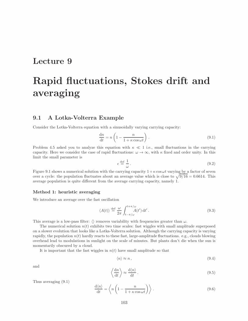
Lecture 9

Rapid fluctuations, Stokes drift and

averaging

9.1 A Lotka-Volterra Example

Consider the Lotka-Volterra equation with a sinusoidally varying carrying capacity:

dn

dt= n

(

1− n

1 + κ cosωt

)

. (9.1)

Problem 4.5 asked you to analyze this equation with κ ≪ 1 i.e., small fluctuations in the carryingcapacity. Here we consider the case of rapid fluctuations: ω → ∞, with κ fixed and order unity. In thislimit the small parameter is

ǫdef=

1

ω. (9.2)

Figure 9.1 shows a numerical solution with the carrying capacity 1+κ cosωt varying by a factor of sevenover a cycle: the population fluctuates about an average value which is close to

√

9/16 = 0.6614. Thisaverage population is quite different from the average carrying capacity, namely 1.

Method 1: heuristic averaging

We introduce an average over the fast oscillation

〈A(t)〉 def=

ω

2π

∫ t+π/ω

t−π/ω

A(t′) dt′ . (9.3)

This average is a low-pass filter: 〈〉 removes variability with frequencies greater than ω.The numerical solution n(t) exhibits two time scales: fast wiggles with small amplitude superposed

on a slower evolution that looks like a Lotka-Volterra solution. Although the carrying capacity is varyingrapidly, the population n(t) hardly reacts to these fast, large-amplitude fluctuations. e.g., clouds blowingoverhead lead to modulations in sunlight on the scale of minutes. But plants don’t die when the sun ismomentarily obscured by a cloud.

It is important that the fast wiggles in n(t) have small amplitude so that

〈n〉 ≈ n , (9.4)

and ⟨dn

dt

⟩

≈ d〈n〉dt

. (9.5)

Thus averaging (9.1)d〈n〉dt

=

⟨

n

(

1− n

1 + κ cosωt

)⟩

. (9.6)

103

0 5 10 15 20 25 300

0.2

0.4

0.6

0.8

t

N(t)

Figure 9.1: An ode45 solutionof the Lotka-Volterra equation(9.1) with ω = 20 and κ =3/4. The blue line indicates√1− κ2 =

√7/4.

But the fast oscillations in n(t) have small amplitude, so

⟨

n

(

1− n

1 + κ cosωt

)⟩

≈ 〈n〉(

1−⟨

1

1 + κ cosωt

⟩

〈n〉)

. (9.7)

The average of the reciprocal carrying capacity is calculated by invoking a favourite textbook exampleof the residue theorem

1

2π

∫ 2π

0

dτ

1 + κ cos τ=

1√1− κ2

. (9.8)

Putting it all together, (9.6) becomes

d〈n〉dt

≈ 〈n〉(

1− 〈n〉√1− κ2

)

. (9.9)

Thus, the long time limit is

limt→∞

〈n〉 →√

1− κ2 . (9.10)

This prediction is in agreement with the matlab solution in Figure 9.1.

Method 2: two-timing

Define a fast time

τdef= ωt =

t

ǫ, (9.11)

and assume that the solution has the multiple time scale expansion

n = n0(t, τ) + ǫn1(t, τ) + · · · (9.12)

depending on both t and τ . Thus the expanded version of (9.1) is

(∂τ + ǫ∂t) (n0 + ǫn1) = ǫn0

(

1− n0

1 + κ cos τ

)

+ ord(ǫ2), (9.13)

and at leading orderǫ0 : ∂τn0 = 0 , with solution n0 = g(t) . (9.14)

We decide to define g(τ) so that all subsequent terms in the expansion have zero average i.e.,

g = 〈n〉 . (9.15)

This definition has the implication that g(t) does not satisfy the initial condition on n(t) i.e., g(0) 6= n(0).(See the discussion of the “guiding center” in section 9.3.)

At next order

ǫ1 : ∂τn1 +dg

dt= g

(

1− g

1 + κ cos τ

)

. (9.16)

104

Using (9.8), we average the equation above over the fast time scale to obtain

dg

dt= g

(

1− g√1− κ2

)

. (9.17)

This confirms the earlier heuristic average.To determine the fluctuations about this average g(t) we can subtract (9.17) from (9.16) to obtain

∂τn1 =

(1√

1− κ2− 1

1 + κ cos τ

)

g2 . (9.18)

To perform the integration and obtain n1(τ) one can invoke the Fourier series

1√1− κ2

− 1

1 + κ cos τ= − 2√

1− κ2

∞∑

n=1

(√1− κ2 − 1

κ

)n

cosnτ . (9.19)

This may be more than we need to know. The main point is that the fast fluctuations about the meansolution g(t) scale with ω−1 i.e., faster fluctuations in the carrying capacity induce smaller variations inpopulation.

9.2 The averaging theorem

There is theorem1 that can be used to justify the method of averaging. Consider the differential equation

dx

dt= ǫf(x, t, ǫ) , (9.20)

where f is periodic in time with period p:

f(x, t+ p, ǫ) = f(x, t+ p, ǫ) . (9.21)

With enough assumptions regarding the smoothness of f , there exists an ǫ0 > 0 and a function u(x, t, ǫ)such that if |ǫ| < ǫ0 then the change of variables

x = y + ǫu(x, t, ǫ) , (9.22)

transforms (9.20) intody

dt= ǫf(y) + ǫ2f1(y, t, ǫ) . (9.23)

In (9.23)

f(y)def=

1

p

∫ p

0

f(y, t, 0) dt (9.24)

is the average of f . The change of variables from x to y in (9.22) is a near-identity transformation thattakes (9.20) into (9.23) exactly. Neglecting the ǫ2 term in (9.23) we obtain an approximate autonomousdifferential equation

dz

dt= ǫf(z) . (9.25)

We hope that the solution z(t) of (9.25) approximates the solution y(t) of (9.23) over some long timeinterval. This hope is justified if the solutions of (9.23) are stable when subject to small, order ǫ2,persistent perturbations.

Example: Considerdx

dt= −αx cosωt . (9.26)

Example: Considerdx

dt= −α(x+ cos2 ωt) . (9.27)

1See Sanders & Verhulst Averaging Methods in Nonlinear Dynamical Systems

105

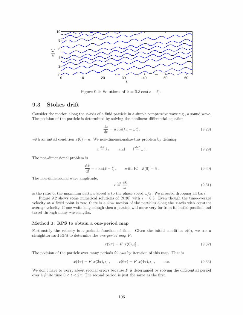
0 10 20 30 40 50 600

2

4

6

8

10

t

x(t)

Figure 9.2: Solutions of x = 0.3 cos(x− t).

9.3 Stokes drift

Consider the motion along the x-axis of a fluid particle in a simple compressive wave e.g., a sound wave.The position of the particle is determined by solving the nonlinear differential equation

dx

dt= u cos(kx− ωt) , (9.28)

with an initial condition x(0) = a. We non-dimensionalize this problem by defining

xdef= kx and t

def= ωt . (9.29)

The non-dimensional problem is

dx

dt= ǫ cos(x− t) , with IC x(0) = a . (9.30)

The non-dimensional wave amplitude,

ǫdef=

uk

ω, (9.31)

is the ratio of the maximum particle speed u to the phase speed ω/k. We proceed dropping all bars.Figure 9.2 shows some numerical solutions of (9.30) with ǫ = 0.3. Even though the time-average

velocity at a fixed point is zero there is a slow motion of the particles along the x-axis with constantaverage velocity. If one waits long enough then a particle will move very far from its initial position andtravel through many wavelengths.

Method 1: RPS to obtain a one-period map

Fortunately the velocity is a periodic function of time. Given the initial condition x(0), we use astraightforward RPS to determine the one-period map F :

x(2π) = F [x(0), ǫ] . (9.32)

The position of the particle over many periods follows by iteration of this map. That is

x(4π) = F [x(2π), ǫ] , x(6π) = F [x(4π), ǫ] , etc. (9.33)

We don’t have to worry about secular errors because F is determined by solving the differential periodover a finite time 0 < t < 2π. The second period is just the same as the first.

106

Method 2: two-timing

To analyze this problem with multiple scale theory we introduce

sdef= ǫ2t . (9.34)

Why ǫ2 above? Because we tried ǫ1 and found that there were no secular terms on this time scale.

Exercise: Assume that s = ǫt and repeat the following calculation. Does it work?

With the slow time s, the dressed-up problem is

ǫ2xs + xt = ǫ cos(x− t) . (9.35)

We now go to town with the RPS:

x = x0(s, t) + ǫx1(s, t) + ǫ2x2(s, t) + · · · (9.36)

Notice that

cos(x− t) = cos(x0 − t)− sin(x0 − t)[ǫx1(s, t) + ǫ2x2(s, t) + · · ·

]

− cos(x0 − t)[ǫx1(s, t) + ǫ2x2(s, t) + · · ·

]2+ · · · (9.37)

We cannot assume that x0 is smaller than one, so must keep cos(x0− t) and sin(x0− t). We are assumingthe higher order xn’s are bounded, and since ǫ≪ 1 we can expand the sinusoids as above.

At leading order, ǫ0:x0t = 0 , ⇒ x0 = f(s) . (9.38)

The function f(s) is the slow drift. At next order, ǫ1:

x1t = cos(f − t) ⇒ x1 = sin f − sin(f − t) . (9.39)

We determined the constant of integration above so that x1 is zero initially i.e., we are saying that f(0)is equal to the initial position of the particle.

At ǫ2

fs + x2t = − sin(f − t) [sin f − sin(f − t)]︸ ︷︷ ︸

=x1

. (9.40)

Averaging over the fast time t we obtain

fs =⟨sin2(f − t)

⟩=

1

2. (9.41)

Thus the average position of the particle is

f =s

2+ a =

ǫ2

2t+ a . (9.42)

The prediction is that the averaged velocity in figure 9.2 is (0.3)2/2 = 0.045. You can check this bynoting that the final time is 20π.

Subtracting (9.41) from (9.40) we have the remaining oscillatory terms:

x2t = − sin(f − t) sin f − sin(2f − 2t) . (9.43)

Integrating and applying the initial condition we have

x2 = − cos(f − t) sin f + 14 cos(2f − 2t) + cos f sin f − 1

4 cos 2f . (9.44)

This is bounded and all is well.The solution we’ve constructed consists of a slow drift and a rapid oscillation about this slowly

evolving mean position. Note however that the mean position of the particle is

〈x〉 = f + ǫ sin f︸︷︷︸

〈x1〉

+ǫ2[12 sin 2f − 1

4 cos 2f]

︸ ︷︷ ︸

〈x2〉

+ord(ǫ2) (9.45)

In other words, the mean position is not the same as the leading-order term.

107

Method 3: two-timing and the “guiding center”

In this variant we use the two-timing but insist that the leading-order term is the mean position of theparticle. This means that the leading-order solution no longer satisfies the initial condition, and thatconstants of integration at higher orders are determined by insisting that

∀n ≥ 1 : 〈xn〉 = 0 . (9.46)

OK, let’s do it, starting with the scaled two-time equation in (9.35). The leading order is

x0t = 0 , ⇒ x0 = g(s) . (9.47)

The function g(s) is the “guiding center” — it’s different from f(s) in the previous method.At next order, ǫ1:

x1t = cos(g − t) ⇒ x1 = − sin(g − t) . (9.48)

This is not the same as the first-order term in (9.39): in (9.48) we have determined the constant ofintegration so that 〈x1〉 = 0.

At order ǫ2 we havegs + x2t = sin2(g − t) = 1

2 − 12 cos(2g − 2t) . (9.49)

The average of (9.49) is the motion of the guiding center:

gs =12 ⇒ g =

ǫ2

2t+ g(0) . (9.50)

The oscillatory part of the solution, with zero time average, is

x2 = 14 sin(2g − 2t) . (9.51)

Now we must satisfy the initial conditions by requiring that

a = g(0)− ǫ sin (g(0)) + ǫ2 14 sin (2g(0)) + · · · (9.52)

We can invert this series to obtaing(0) = a+ ǫ sina+ · · · (9.53)

I prefer this guiding center method. But in either case the essential point is that the leading-order driftvelocity is ǫ2/2.

9.4 The Kapitsa pendulum

If you google the “Kapitsa pendulum” you’ll find videos which show the stabilization of an invertedpendulum by a rapidly vibrating point of support. The equation of motion of this system is

d2ϕ

dt2+

(g

ℓ+aν2

ℓcos νt

)

sinϕ = 0 , (9.54)

where a is the amplitude of vibration and ν is the frequency. There is a steady solution ϕ = π and inthe absence of vibration (a = 0) this solution is unstable.

Let’s scale the equation and show that if ν is large enough then solution ϕ = π becomes stable. Webegin the analysis by introducing a nondimensional time

tdef= ωt , (9.55)

where ωdef=√

g/ℓ is the linear frequency of the pendulum. The non-dimensional equation of motion canthen be written as

d2ϕ

dt2+

[

1 +α

ǫcos

(t

ǫ

)]

sinϕ = 0 , (9.56)

108

whereǫdef=

ω

ν, and α

def=

aων

g. (9.57)

To investigate the stability of ϕ = π we introduce θ = π − ϕ so that

sinϕ = − sin θ = −θ + ord(θ3) . (9.58)

Dropping the bar on the nondimensional time, the linearized problem is

d2θ

dt2−(

1 +α

ǫcos

(t

ǫ

))

θ = 0 . (9.59)

We take the distinguished limit ǫ→ 0 with α fixed.Introduce the fast time τ = t/ǫ so that

d

dt=

1

ǫ∂τ + ∂t , (9.60)

and use the two-time expansionθ = θ0(t, τ) + ǫθ1(t, τ) + · · · (9.61)

The expanded equation of motion is

(∂τ + 2ǫ∂t∂τ + ǫ2∂2t

) (θ0 + ǫθ1 + ǫ2θ2

)− ǫ2θ0 − ǫα cos τ (θ0 + ǫθ1) = ord

(ǫ3). (9.62)

At order ǫ0 we have∂2τθ0 = 0 , ⇒ θ0 = S(t) . (9.63)

Above, at leading order, the leading order displacement is a function of only the slow time t. At nextorder ǫ1:

∂2τθ1 + 2 ∂t∂τS︸ ︷︷ ︸

=0

−αS cos τ = 0 , ⇒ θ1 = −αS cos τ . (9.64)

At order ǫ2:∂2τθ2 + 2 ∂t∂τθ1

︸ ︷︷ ︸

αSt sin τ

+∂2t S − S − α cos τ θ1︸ ︷︷ ︸

−α2S cos2 τ

= 0 . (9.65)

Averaging the equation above we find that

Stt −(1− 1

2α2)S = 0 . (9.66)

The inverted pendulum is stable if α >√2.

9.5 Problems

Problem 9.1. Consider the nonlinear inverted pendulum

d2θ

dt2−[

1 +α

ǫcos

(t

ǫ

)]

sin θ = 0 . (9.67)

Apply the two-time method to this nonlinear equation and find the effective potential resulting fromaveraging the rapid oscillations. Calculate the phase-plane orbits in the effective potential.

109

-1.5 -1 -0.5 0 0.5 1 1.5

x

-1.5

-1

-0.5

0

0.5

1

1.5y

Figure 9.3: The solid curveis the numerical solution of(9.68), with ω = 8; the ini-tial condition is indicated bythe blue ∗; the system hasbeen integrated from t = 0to t = 203.7 × 2π/8 i.e., al-most 204 periods of cosωt. Theblack dashed curve is the guid-ing center.

Problem 9.2. A solution of

dx

dt= sinωt cos y ,

dy

dt= cosωt cosx , (9.68)

with ω = 8 and initial condition [x(0), y(0)] = [1.1, 0] is shown in figure 9.3. Find an expression for thetrajectory of the guiding center (the black dashed curve).

Problem 9.3. As a generalization of problem 9.2, investigate Stokes drift in the two-dimensional in-compressible velocity field with streamfunction

ψ = a(x, y) cos(t/ǫ) + b(x, y) sin(t/ǫ) , (9.69)

and velocitydx

dt= −ψy ,

dy

dt= ψx . (9.70)

Obtain an expression for the streamfunction of the Stokes flow.

110

−40 −30 −20 −10 0 10 20 30 40−4

−2

0

2

4

t

x(t)andx(t)

−40 −30 −20 −10 0 10 20 30 400

1

2

3

4

5

t

A(t),E(t)andω(t)

ǫ = 0.25Figure 9.4: Solution of (9.71)and (9.72) with ode45. Inthe lower panel the red dashedcurve is ω(t), the black curveis the energy E(t) and the al-most constant action is the bluedashed curve.

Problem 9.4. Consider an oscillator with a slowly changing frequency ω(ǫt):

x+ ω2x = 0 . (9.71)

Use the method of averaging to show that the action Adef= E/ω is approximately constant. Test this

result with ode45 using the frequency

ω(t) = 3 + 2 tanh (ǫt) , (9.72)

and the initial condition x(−40) = 0 and x(−40) = 1 e.g., see Figure 9.4. Use several values of ǫ to testaction conservation e.g., try to break the constant-action approximation with large ǫ.

111

0 20 40 60 80 100 120

t

-2

-1

0

1

2

x(t)an

dy(t)

ǫ = 0.05

Figure 9.5: Numerical solution of (9.73).

Problem 9.5. A multiple scale (0 < ǫ≪ 1) reduction of the crazy oscillator

d2x

dt2+ 2ǫy

dx

dt+ x = 0 ,

dy

dt= 1

2ǫx2 , (9.73)

begins with

x =[A(s)eit +A∗(s)e−it

]+ ǫx1(t, s) + · · · , y = B(s) + ǫy1(t, s) + · · · (9.74)

where s = ǫt is the slow time. (i) Find coupled evolution equations for A(s) and B(s). (ii) Figure 9.5shows a numercial solution of (9.73) with the initial conditions

x(0) = 2 ,dx

dt(0) = 0 , y(0) = 0 . (9.75)

Explain why limt→∞ y = 1.

112

Lecture 10

Eigenvalue problems

10.1 Regular Sturm-Liouville problems

The second-order differential equation associated with a Sturm-Liouville eigenproblem has the form

(pφ′)′ − qφ+ λwφ = 0 , (10.1)

where p(x), q(x) and r(x) are real functions. The associated boundary value problem is posed ona < x < b with BCs which we write as

αφ(a)− α′φ′(a) = 0 , and βφ(b) + β′φ′(b) = 0 , (10.2)

where [α, α′, β, β′] are real constants.The sign convention in (10.2) is so that (10.27) below looks pretty. In physical problems, such as

radiation of heat through the boundaries at x = a and b, the mixed boundary condition is

dφ

dn+ (a positive constant)× φ = 0 , (10.3)

where n is the outwards normal at the boundary. At x = a < b the outwards normal implies n = −x.Thus if [α, α′, β, β′] are all positive then the boundary conditions in (10.2) conform to (10.3) at x = aand b.

Example: The archetypical SL eigenproblem with Dirichlet boundary conditions is:

− φ′′ = λφ with BCs φ(0) = φ(π) = 0 . (10.4)

Prove that λ ≥ 0 before attempting a solution.

Example: The archetypical SL eigenproblem with Neuman boundary conditions is:

− φ′′ = λφ , with BCs φ′(0) = φ′(π) = 0 . (10.5)

Prove that λ ≥ 0 before attempting a solution.

Example: A soluble example with non-constant coefficients:

− φ′′ = λx−2φ , with BCs φ(1) = φ(ℓ) = 0 . (10.6)

First we prove that λ ≥ 0. The differential equation is an Euler equation which can be solved with φ = xν .Thus we find that

ν2 − ν + λ = 0 , or ν = 12±√

14− λ . (10.7)

We have to consider two cases: (a) λ < 1/4 and (b) λ > 1/4. In case (a) we have two real ν’s, but thereis no way to combine these into a solution that satisfies the boundary conditions. So we turn to case (b),for which

λ = 12± i√

λ− 14

(10.8)

113

1 1.2 1.4 1.6 1.8 2 2.2 2.4 2.6 2.8 3−2

−1

0

1

2

x

φn(x

)

Figure 10.1: The first five Sturm-Liouville eigenfunctions in (10.12)with ℓ = 3.

and

xν = x1/2

[

cos

(√

λ− 14ln x

)

± i sin

(√

λ− 14ln x

)]

(10.9)

We can linearly combine the two solutions above to obtain a solution satisfying the BC at x = 1

φ = x1/2 sin

(√

λ− 14ln x

)

(10.10)

The second boundary condition at x = ℓ > 1 determines the eigenvalue

λ = 14+( nπ

ln ℓ

)2

, (10.11)

and therefore

φ = x1/2 sin

(

nπlnx

ln ℓ

)

. (10.12)

The first five eigenfunctions are shown in figure 10.1. Notice that the n’th eigenfunction has n−1 interiorzeros.

Example: We’ll use the SL problem− φ′′ = λxφ (10.13)

as an Airy-function reminder. The problem is posed on the interval 0 < x < ℓ with Dirichlet boundaryconditions

φ(0) = φ(ℓ) = 0 . (10.14)

This SL problem is a little irregular because the weight function is zero at x = 0. But, once again, we canshow that λ is positive. The analytic solution of (10.13) is

φ =Ai(

−xλ1/3)

Ai(0)−

Bi(

−xλ1/3)

Bi(0). (10.15)

It is certainly reassuring to know that λ1/3 in the equation above is a real positive number. The construc-tion above satisfies both the differential equation and the boundary condition at x = 0. The boundarycondition at x = ℓ produces the eigenrelation

Ai (−η)Ai(0)

=Bi (−η)Bi(0)

, (10.16)

where ηdef= ℓλ1/3. If you look at the graphs of the Airy and Bairy function in the upper panel of Figure

10.2 then you can anticipate that this eigenrelation has an infinite number of solutions. The first five are

ℓλ1/3 = [2.6664 , 4.3425 , 5.7410 , 6.9861 , 8.1288] , (10.17)

and the lower panel of Figure 10.2 shows the corresponding eigenfunctions. Again, notice that the n’theigenfunction has n− 1 interior zeros.

10.2 Properties of Sturm-Liouville eigenproblems

We write the differential equation in (10.1) as

Lφ = λwφ , (10.18)

114

0 1 2 3 4 5 6 7 8 9 10−2

−1

0

1

2

ℓ/λ1/3

Airyfu

nctions

0 0.1 0.2 0.3 0.4 0.5 0.6 0.7 0.8 0.9 1−2

−1

0

1

2

x/ℓ

φn(x

)

Figure 10.2: The upper panel showsthe two Airy functions on the rightof (10.16); each intersection corre-sponds to an eigenvalue. The lowerpanel shows the first five eigenfunc-tions corresponding to the eigenval-ues in (10.17).

where L is the second-order differential operator

Ldef= − d

dxpd

dx+ q . (10.19)

L is defined with the minus sign so that if p is a positive function then L is a positive operator.The operator L is hungry, looking for a function to differentiate. If p(x) > 0 and w(x) > 0 on [a, b]

and p, q and w are all free from bad singularities, then the problem is regular.The main results for regular problems are:

1. The eigenvalues are real, countable and ordered so that there is a smallest one

λ0 < λ1 < λ2 < · · · (10.20)

Moreover limn→∞ λn = ∞.

2. The zeroth eigenfunction (also known as the gravest mode, or the ground state) has no interiorzeroes. Eigenfunction φn+1(x) has one more interior zero than φn(x).

3. Eigenfunctions with different eigenvalues are orthogonal with respect to the weight function w:

∫ b

a

φm(x)φn(x)w(x) dx = ξnδmn . (10.21)

Often, but not always, we normalize the eigenfunctions so that ξn = 1.

4. Within (a, b), any square integrable1 function f(x) can be represented as

f(x) =

∞∑

n=1

fnφn(x) , (10.22)

with

fn = ξ−1n

∫ b

a

φn(x)f(x)w(x) dx . (10.23)

1Square integrable means with respect to the weight function. That is

∫ b

a

f2wdx <∞ .

115

5. Considering the truncated sum

fN (x) =

N∑

n=1

fnφn(x) , (10.24)

as an approximation to the target function f(x), we define the error in fN (x) as

e(f1, f2, · · · fN )def=

∫ b

a

[

f −N∑

n=1

fnφn

]2

w dx . (10.25)

If we adjust f1 through fN to minimize the error e then we recover the expression for fn in (10.23).Moreover

limN→∞

e = 0 . (10.26)

Eigenvalue are real

To prove that all eigenvalues are real, multiply (10.1) by φ∗(x) and integrate over the interval. With IPwe find

λ =

∫ b

ap|φ′|2 + q|φ|2dx+ βp(b)|φ′(b)|2 + αp(a)|φ′(a)|2

∫ b

a |φ|2w dx, (10.27)

where βdef= β′/β and α

def= α′/α. The right hand side — which is manifestly real — is known as the

Rayleigh quotient. If q(x), α and β are all non-negative then the Rayleigh quotient also shows that theeigenvalues are positive.

Exercise: how does (10.27) change if β = 0 and/or α = 0?

Eigenfunctions are orthogonal

To prove orthogonality above we first prove

uLv − vLu = [p(vu′ − uv′)]′, (10.28)

and therefore∫ b

a

uLv dx−∫ b

a

vLu dx =[p(vu′ − v′u)

]b

a. (10.29)

Exercise: use the identity above to prove (10.21)

The eigenfunction expansion minimizes the squared error

Exercise: prove that fn in (10.23) minimizes e(f1, f2, · · · fN ) in (10.25).

Example: expand f(x) = 1 in terms of sinnx (again).

10.3 Trouble with BVPs

Not all BVPs have solutions. An example is the thermal diffusion problem

ψt = ψxx + 1 , (10.30)

posed on 0 < x < 1 with insulating boundary conditions

ψx(0, t) = ψx(1, t) = 0 . (10.31)

For obvious reasons there are no steady solutions to this partial differential equation: the BVP

− ψxx = 1 , with ψx(0) = ψx(1) = 0 , (10.32)

116

has no solutions. To see this mathematically, integrate the differential equation in (10.32) from x = 0to x = 1:

− [ψx]10

︸ ︷︷ ︸

=0

= 1 . (10.33)

The contradiction tells us not to bother looking for a steady solution to (10.30). Instead, we should

solve the diffusion equation (10.30) with the ansatz ψ = t + ψ(x, t), where ψ is required to satisfy theinitial conditions.

Exercise: show that limt→∞ ψ = 0 .

In other examples, the non-existence of solutions is less obvious. Consider the example

y′′ + y = lnx , with y(0) = y(π) = 0 . (10.34)

If we multiply the differential equation by sinx and integrate from x = 0 to π then, with some IP, wequickly obtain

∫ π

0

sinx (y′′ + y) dx

︸ ︷︷ ︸

=0

=

∫ π

0

sinx lnxdx = 0.641182 . (10.35)

Again, the contradiction tells us that there is no point in looking for a solution.We can write (10.34) using fancy operator notation as

Ly = ln1

x, where L

def= − d2

dx2− 1. (10.36)

Now let’s do the calculation using some Sturm-Liouville machinery: Multiply by sinx, integrate over theinterval, use the identity (10.28) and use the fact that sinx and y are zero on both boundaries. Thusagain we obtain the contradiction

∫

y L sinx︸ ︷︷ ︸

=0

dx =

∫ π

0

sinx ln xdx (10.37)

It’s the same calculation as before. You should get used to seeing that

∫

uLvdx =

∫

vLudx . (10.38)

If you use the identity above be sure to check that the boundary conditions imply that all the termsfalling outside the integral are zero! Go back to (10.28) and see what’s required for that to happen.....

More generally we might confront

y′′ + y = f(x) , with y(0) = y(π) = 0 , (10.39)

where f(x) is some function. If we multiply the differential equation by sinx and integrate from x = 0to π we have ∫ π

0

sinxf(x) dx = 0 . (10.40)

In order for a solution of (10.39) to exist, the solvability condition in (10.40) must be satisfied. Andif (10.40) is satisfied then (10.39) has an infinity of solutions: if y(x) is a solution of (10.39) theny(x) + a sinx is also a solution for every value of the constant a.

To understand what’s going on here, we turn to the eigenfunction expansion method.

117

10.4 The eigenfunction expansion method

Suppose that somehow we have solved the eigenvalue problem

Lφ = λwφ , (10.41)

with BCs φn(a) = φn(b) = 0. This means we possess the full spectrum λn and φn(x) with n = 0, 1 · · ·The solution of the boundary value problem

Ly = f , (10.42)

with BCs y(a) = 0 and y(b) = 0, is represented as

y(x) =

∞∑

n=0

ynφn(x) , with ym = ξ−1m

∫ b

a

φmy w dx . (10.43)

Multiply (10.42) by φm(x) and integrate over the interval. Using the identity in (10.28), and theboundary conditions, the left hand side of (10.42) produces

∫ b

a

φmLy dx =

∫ b

a

yLφm dx ,

= λm

∫ b

a

yφmw dx ,

= λmξmym . (10.44)

Thus

ym =

∫ b

a φmf dx

λmξm(10.45)

This is OK provided that all the eigenvalues are non-zero. If there is a zero eigenvalue then this problemhas no solution.

Example: Solvey′′ = ln x (10.46)

with y(0) = y(π) = 0. In this example the weight function is w(x) = 1 and

L = − d2

dx2, φn = sin nx , λn = n2 , (10.47)

with n = 1, 2 · · · There are no zero modes, and therefore there is no problem with existence of thesolution. The expansion coefficients are

yn = − 2

πn2

∫ π

0

sinnx lnx dx . (10.48)

Evaluating the integral in (10.48) numerically, we find that the first six terms in the series solution are

y1 = −0.408189 sin x+ 0.193982 sin 2x+ 0.0122721 sin 3x

+ 0.0309791 sin 4x+ 0.0052863 sin 5x+ 0.0103642 sin 6x+ · · · (10.49)

Figure 10.3 compares the exact solution of this BVP, namely

y = 12x2 ln x− 1

2πx lnπ +

3

4

(πx− x2) , (10.50)

with (10.49) truncated with 2, 4 and 6 terms.

118

0 0.5 1 1.5 2 2.5 3

−0.5

−0.4

−0.3

−0.2

−0.1

0

0.1

x

y(x

)

Figure 10.3: Comparison of the exact solution (10.50) (the solid curve) with truncations of theseries (10.49). The two-term truncation is the green dashed curve, the four-term truncation isthe red dash-dot curve and the six term truncation is the dotted cyan curve.

Example: Reconsider our earlier example

y′′ + y︸ ︷︷ ︸

−Ly

= ln x , with BCs y(0) = y(π) = 0 . (10.51)

We first find the eigenspectrum by solving

Lφ = λφ φ(0) = φ(π) = 0 . (10.52)

The eigenfunctions areφn(x) = sinnx , n = 1 , 2 , 3 , · · · (10.53)

with eigenvaluesλn = n2 − 1 = 0, 1, 3, 8 · · · (10.54)

Oh oh, there is a zero eigenvalue. So there is no solution.

Example: Find a so that the problem

y′′ + y = ln x+ a , with BCs y(0) = y(π) = 0 , (10.55)

has a solution. Construct the most general solution as an eigenfunction expansion.

We know that sin x is a zero-eigenmode, and therefore the solvability condition is

0 =

∫ π

0

(lnx+ a) sin xdx implying that a =

∫ π

0sin x ln 1

xdx

∫ π

0sin xdx

= −0.320591 . (10.56)

Now we can solve the problem using the eigenmodes defined by the SL problem

−(

d2

dx2+ 1

)

︸ ︷︷ ︸

L

φ = λφ , with φ(0) = φ(π) = 0 . (10.57)

The eigenvalues are

λn = n2 − 1 , with eigenfunction φn(x) = sinnx . (10.58)

Operationally, we multiply (10.55) by sinmx and integrate over the interval from x = 0 to π. Thus

(1−m2)

∫ π

0

y sinmxdx

︸ ︷︷ ︸π2ym

=

∫ π

0

(ln x+ a) sinmxdx , with m = 2, 3, · · · (10.59)

The solution of the BVP is

y = A sin x− 2

π

∞∑

n=2

∫ π

0(ln x+ a) sinnxdx

n2 − 1sin nx , (10.60)

where A is an arbitrary constant.

119

Exercise: Show that the BVP

y′′ = ln x , with BCs y′(0) = y′(π) = 0 , (10.61)

has no solution. Determine a so that the related BVP

y′′ = lnx+ a , with BCs y′(0) = y′(π) = 0 , (10.62)

has a solution. Find the most general solution of this problem by direct integration, and by the eigen-function expansion method.

10.5 Eigenvalue perturbations

Consider a string with slightly non-uniform mass density

ρ(x) = ρ0 [1 + ǫb(x)] . (10.63)

We compute the change in the eigenfrequencies induced by the small non-uniformity in density.Using nondimensional variables, the eigenproblem is

ψ′′ + λ(1 + ǫb)ψ = 0 , (10.64)

with ψ(0) = ψ(π) = 0.First suppose that ǫ = 0. We quickly see that the solution of the ǫ = 0 eigenproblem is

λ = k2 , with corresponding eigenfunction sk(x)def=

√

2

πsin kx , (10.65)

where k = 1, 2 · · · is the mode number.Let’s focus on mode number m and ask how the eigenvalue m2 changes when ǫ 6= 0? We use the

RPSψ = ψ0

︸︷︷︸

=sm

+ǫψ1 + · · · and λ = λ0︸︷︷︸

m2

+ǫλ(1) + · · · (10.66)

Although it is not strictly necessary, it helps to normalize the perturbed eigenfunction so that∫ π

0

ψ2 dx = 1 . (10.67)

Expansion of the normalization above implies∫ π

0

ψ20 dx = 1 ,

∫ π

0

ψ0ψ1 dx = 0 ,

∫ π

0

2ψ0ψ2 + ψ21 dx = 0 , etc. (10.68)

The expressions above will simplify the appearance of subsequent formulas.The first three orders of the perturbation hierarchy are

Lψ0 = 0 , (10.69)

Lψ1 = (λ1 + λ0b)ψ0 , (10.70)

Lψ2 = (λ2 + λ1b)ψ0 + (λ1 + λ0b)ψ1 . (10.71)

Above,

Ldef= − d2

dx2− λ0︸︷︷︸

=m2

, (10.72)

is the “unperturbed operator”.Notice that (10.69) says that L has a zero eigenvalue with the zero-mode sm. Thus there is a problem

with solving boundary value problems of the form

Lf = some function of x , (10.73)

120

with f(0) = f(π) = 0. For a solution to exist, the right hand side must be orthogonal to ψ0 = sm. Thusto ensure that (10.70) and (10.71) have solutions, one requires

λ1 = −m2

∫

bs2m dx , (10.74)

λ2 = −λ1∫

bs2m dx−m2

∫

bsmψ1 dx , (10.75)

and so on. (All integrals are from 0 to π.) Notice how the expansion of the eigenvalue is obtained byenforcing the solvability condition order by order.

The first-order shift in the m’th eigenvalue is given by (10.74). If the density in the middle of thestring is increased then the eigenfrequency is decreased.

Exercise: At one point in the calculation above (10.68) was used to simplify an expression. Where was that?

The second-order terms

The second-order correction from (10.75) can be written as

λ2 =λ21m2

−m2

∫

bsmψ1 dx . (10.76)

To get λ2, we have to solve (10.70) for ψ1 and then substitute into (10.76). Using the modal projectionmethod, the solution of (10.70) is

ψ1(x) = m2∞∑

n=1, 6=m

Jmnsn(x)

n2 −m2, (10.77)

where the sum over n above does not include the singular term, n = m, and

Jmndef=

∫ π

0

bsmsn dx . (10.78)

Thus the second-order shift in the eigenvalue is

λ2 =λ21m2

−m4∞∑

n=1

J2mn

n2 −m2. (10.79)

10.6 The vibrating string

A physical example is a string with uniform tension T (in Newtons) and mass density ρ(x) (kilogramsper meter) stretched along the axis of x. The wave speed is

cdef=

√

T

ρ. (10.80)

After linearization the transverse displacement η(x, t) satisfies

ρηtt − Tηxx = −ρg + f . (10.81)

Above f(x, t) is an externally imposed force (in addition to gravity g). If the string is stretched betweentwo supports at x = 0 and ℓ then the BCs are

η(0) = 0 , and η(ℓ) = 0 . (10.82)

We remove the “static sag” viaη(x, t) = ηs(x) + u(x, t) , (10.83)

121

where the static solution ηs(x) is determined by solving

ηsxx =ρg

T(10.84)

with ηs = 0 at the boundaries.

Exercise: Show that if ρ is constant

ηs(x) = − ρg

2Tx(ℓ− x) . (10.85)

Thus the disturbance, u(x, t), satisfies

ρutt − Tuxx = f . (10.86)

If f = 0 there is a special class of “eigensolutions” which we find with the substitution

u(x, t) = φ(x)e−iωt . (10.87)

This produces a typical SL eigenproblem

Tφxx + ω2ρφ = 0 , (10.88)

with BCs φ(0) = φ(ℓ) = 0 inherited from (10.82).

Example: Suppose that ρ is uniform so that the wave speed, c =√T/ρ, is a constant. the spectrum is therefore

φn(x) = sin knx , with eigenfrequency ωn =nπc

ℓ. (10.89)

The wavenumber above is kn = ωn/c = nπ/ℓ.

Exercise: Solve the problem above with a free boundary at x = ℓ: i.e., the boundary condition is changed toux(ℓ) = 0 .

After we solve (10.88) we possess a set of complete orthogonal functions, φn(x) each with a corre-sponding eigenfrequency. The orthogonality condition is

∫ ℓ

0

φpφqρ dx = βpδpq , (10.90)

where βp is a normalization constant. (Often, but not always, we make βp = 1.)Returning to the forced problem in (10.86) we build the solution of this partial differential equation

as linear superposition of the eigenmodes

u(x, t) =

∞∑

m=1

um(t)φm(x) . (10.91)

Using orthogonality, the modal amplitude is given by

βnun(t) =

∫ ℓ

0

u(x, t)φn(x)ρ(x) dx . (10.92)

Evolution equations for the modal amplitudes follow via projection of the equation (10.86) onto themodes i.e., multiply (10.86) by φn(x) and integrate from x = 0 to x = ℓ. After some integration by partsone finds

d2undt

+ ω2nun = β−1

n

∫ ℓ

0

φn(x)f(x, t)dx . (10.93)

If we also represent the forcing f as

f(x, t) = ρ(x)∞∑

m=0

f(t)φm(x) , with βnfn(t) =

∫ ℓ

0

φn(x)f(x, t) dx , (10.94)

122

then we haved2undt2

+ ω2nun = fn . (10.95)

Each modal amplitude, un(t), satisfies a forced harmonic oscillator equation.We declare victory after reducing the partial differential equation (10.86) to a big set of uncoupled

ordinary differential equations in (10.95). This victory is contingent on solving the eigenproblem (10.88)and understanding basic properties of SL problems such as the orthogonality condition in (10.90)

Example: In some problems the tension T is non-uniform and the wave equation is then

ρutt − (Tux)x = f . (10.96)

A nice example is a dangling chain of length ℓ suspended from the point x = 0, with x positive downwards.The tension is then

T (x) = ρg

∫ ℓ

x

ρ(x′) dx′ (10.97)

The BCs η(0) = 0 and ηx(ℓ) = 0.

10.7 Problems

Problem 10.1. (i) Transform

a(x)y′′ + b(x)y′ + c(x)y + d(x)Ey(x) = 0 , (10.98)

with boundary conditions y(α) = y(β) = 0, into the Sturm-Liouville form

[p(x)y′]′+ [q(x) + Ew(x)] y = 0 . (10.99)

Hint: multiply by an integrating factor I(x); determine I(x) by matching up terms. Your answer shouldinclude clear expressions for [p, q, w] in terms of [a, b, c, d]. (ii) Write Bessel’s equation

y′′ + x−1y′ +[E − ν2x−2

]y = 0 (10.100)

in Sturm-Liouville form. (iii) Prove that the eigenfunctions yn(x) associated with (10.99) satisfy

(En − Em)

∫ β

α

yn(x)ym(x)w(x) dx = 0 . (10.101)

Thus if Em 6= En then the eigenfunctions are orthogonal with respect to the weight function r(x).

Problem 10.2. Consider the eigenvalue problem

y′′ = −λy , with BCs: y(0) = 0 , y′(1) = y(1) . (10.102)

(i) Prove that all the eigenvalues are real. (ii) Find the transcendental equation whose solutions de-termine the eigenvalues λn. (iii) Find an explicit expression for the smallest eigenvalue λ0 and theassociated eigenfunction y0(x). (iv) Show that the eigenfunctions are orthogonal with respect to anappropriately defined inner product. (v) Attempt to solve the inhomogeneous boundary value problem

y′′ = a(x), with BCs: y(0) = 0 , y′(1) = y(1) , (10.103)

via an expansion using the eigenmodes. Show that this expansion fails because the problem has nosolution for an arbitrary a(x). (iv) Find the solvability condition on a(x) which ensures that the problem(10.103) does have a solution, and then obtain the solution using a modal expansion.

Problem 10.3. Consider the eigenproblem

− φ′′ = λx−2+ǫφ , with BCs φ(1) = φ(ℓ) = 0 . (10.104)

In the lecture we solved the ǫ = 0 problem and showed that the smallest eigenvalue is

λ1 = 14 +

π

ln ℓ. (10.105)

Find the change in λ1 induced by the perturbation ǫ≪ 1.

123

Problem 10.4. There is a special value of α for which the boundary value problem

y′′ = sinx− α , y′(0) = y′(π) = 0 (10.106)

has a solution. Find the special value of α and in that case solve the boundary value problem by: (i)expansion using a set of eigenfunctions; (ii) explicit solution using a combination of homogeneous andparticular solutions. (iii) Use matlab to compare the explicit solution with a three-term truncation ofthe series solution.

Problem 10.5. Consider the eigenproblem

(a(x)y′)′+ λy = 0 , y′(0) = y′(1) = 0 , (10.107)

where a(x) > 0 for 0 ≤ x ≤ 1. (i) Verify that y(x) = 1 and λ = 0 is an eigensolution. (ii) Showthat λ = 0 is the smallest eigenvalue. (iii) Now consider the perturbed problem in which the boundarycondition at x = 1 is changed to

ǫy(1) + y′(1) = 0 ,

where ǫ is a positive real number. With 0 < ǫ≪ 1, use perturbation theory to determine the O(ǫ) shiftof the λ = 0 eigenvalue. (iii) Obtain the O(ǫ2) term in the expansion of the λ = 0 eigenvalue.

Problem 10.6. (i) Verify that y(x) = 1 and λ = 0 is an eigensolution of

(xy′)′+ λy = 0 , lim

x→0xy′ = 0 , y′(1) = 0 . (10.108)

(ii) Show that λ = 0 is the smallest eigenvalue. (iii) Now consider the perturbed problem in which theboundary condition at x = 1 is changed to

ǫy(1) + y′(1) = 0 ,

where ǫ is a positive real number. With 0 < ǫ≪ 1, use perturbation theory to determine the O(ǫ) shiftof the λ = 0 eigenvalue. (iii) Obtain the O(ǫ2) term in the expansion of the λ = 0 eigenvalue.

Problem 10.7. When ǫ = 0 the eigenproblem

y′′ + ǫyy′ + λy = 0 , y(0) = y(π) = 0 ,

has the solution λ = 1 and y = a sinx. Use perturbation theory (ǫ ≪ 1) to investigate the dependenceof the eigenvalue λ on a and ǫ.

Problem 10.8. Consider a diffusion problem defined on the interval 0 ≤ x ≤ ℓ:

ut = κuxx , u(0, t) = 0 , ux(ℓ, t) = 0 , (10.109)

with initial condition u(x, t) = f(x). (i) If you use separation of variables then it is easy to anticipate thatyou’ll find a Sturm-Liouville eigenproblem with sinusoidal solutions. Sketch the first two eigenfunctionsbefore doing this algebra. Explain why you are motivated to nondimensionalize so that 0 ≤ x ≤ π/2.(ii) With ℓ → π/2 and κ → 1, work out the Sturm-Liouville algebra and find the eigenfunctions andeigenvalues. (iii) With f(x) = 1 find the solution as a Fourier series and use matlab to visualize theanswer.

Problem 10.9. A rod occupies 1 ≤ x ≤ 2 and the thermal conductivity depends on x so that diffusionequation is

ut = (x2ux)x .

The boundary and initial conditions are

u(1, t) = u(2, t) = 0 , u(x, 0) = 1 .

124

(i) The total amount of heat in the rod is

H(t) =

∫ 2

1

u(x, t) dx .

Show that H(0) = 1 anddH

dt= 4ux(2, t)− ux(1, t) .

Physically interpret the two terms on the right hand side above. What is the sign of the ux(2, t) and thesign ux(1, t)? (ii) Before solving the PDE, show that roughly 61% of the heat escapes through x = 2.(There is a simple analytic expression for the fraction 0.61371 · · · which you should find.) (iii) Useseparation of variables to show that the eigenfunctions are

φn(x) =1√xsin

(nπ lnx

ln 2

)

.

Find the eigenvalue which is associated with the n’th eigenfunction. (iv) Use modal orthogonality tofind the series expansion of the initial value problem.

Problem 10.10. Solve the BVP

y′′ + y + ǫf(x)y = 0 , y(0) = 1 , y(π) = 0 , (10.110)

with a perturbation expansion in ǫ; f(x) is some O(1) function. Hint: solve the problem exactly inthe special case f(x) = 1 to infer the form of the perturbation expansion. Is this a regular or singularproblem?

Problem 10.11. Consider the inhomogeneous diffusion equation

ut − uxx =1

√

x(π − x), u(0, t) = u(π, t) = 0 .

(i) Using a modal expansion

u(x, t) =

∞∑

n=1

un(t) sinnx ,

find the ordinary differential equations satisfied by the amplitudes un(t). (ii) Your answer to (i) willinvolve the integral

hn ≡ 2

π

∫ π

0

sinnx√

x(π − x)dx ,

which you probably can’t evaluate off-the-cuff. However you should deduce that hn is zero if n is evenand

hn ≡ 4

π

∫ π/2

0

sinnx√

x(π − x)dx , if n is odd.

Find a leading-order n → ∞ asymptotic approximation of hn. (iii) I believe that un ∼ n−q as n → ∞.Find q.

Problem 10.12. Find the eigenfunction expansion of f(t) = 1 − e−αx in 0 < x < π in terms of theeigenfunctions defined by

u′′ + λu = 0 , with BCs u(0) = u′(π) = 0 . (10.111)

For which values of α is this eigenfunction expansion most effective?

125

Problem 10.13. Solve the eigenproblem

(xu′)′ +3 + λ

xu = 0 , with BCs y(1) = y(2) = 0 . (10.112)

Use these eigenfunctions to solve the inhomogeneous probem

(xy′)′ +3 + λ

xy = sinx with BCs y(1) = y(2) = 0 . (10.113)

Problem 10.14. Use an eigenfunction expansion to solve

d2g

dx2= δ(x− x′) , with BCs g(0, x′) = g(1, x′) = 0 , (10.114)

on the interval 0 < x < 1 for the Green’s function g(x, x′). You can also solve this problem using thepatching method. Remark: considering the inhomogeneous BVP on the interval 0 < x < 1 for y(x):

y′′ = f , with BCs y(0) = y(1) = 0 , (10.115)

we now have two different solution methods: Green’s functions and eigenfunction expansions. Theeigenfunction solution of (10.114) is the connection between these two methods. Can you extend this tothe general SL problem

(pg′)′ + qg = δ(x− x′) with our usual homogenous BCs? (10.116)

Problem 10.15. Use separation of variables to solve the eigenproblem

φxx + φyy︸ ︷︷ ︸

∇2φ

= −λφ . (10.117)

The domain is the π × π square, 0 < (x, y) < π, with the Dirichlet boundary condition u = 0. Thetwo-dimensional Lagrange identity for the operator ∇2 (aka L) is a well-known vector identity. Use thisto prove that the eigenfunctions are orthogonal. Use Galerkin projection and an eigenfunction expansionto solve the inhomogeneous problem

uxx + uyy = 1 , with BCs u = 0 on the square. (10.118)

126

Lecture 11

WKB

11.1 The WKB approximation

Suppose we need to solve1

ǫ2y′′ + q(x)y = 0 , as ǫ→ 0. (11.1)

The approximate WKB solution to this singular perturbation problem is

y ≈ A

q1/4exp

[i

ǫ

∫ x√

q(t) dt

]

+B

q1/4exp

[

− i

ǫ

∫ x√

q(t) dt

]

, (11.2)

or equivalently

y ≈ E

q1/4cos

[1

ǫ

∫ x√

q(t) dt

]

+F

q1/4sin

[1

ǫ

∫ x√

q(t) dt

]

. (11.3)

The constructions above are most convenient if q(x) > 0 so that the solution of (11.1) is oscillatory. ButWKB also works if q(x) < 0 and in that case the approximation is

y ≈ A

|q|1/4 exp

[1

ǫ

∫ x√

|q(t)| dt]

+B

|q|1/4 exp

[

−1

ǫ

∫ x√

|q(t)| dt]

. (11.4)

We have not specified the lower limits of the integrals in (11.1) through (11.4). Different choices amountto altering the constants A, B et cetera.

The approximations in (11.2) through (11.4) fail in the neighbourhood of x∗ where q(x∗) = 0. Thepoint x∗ is called a turning point. We’ll need a different approximation in the vicinity of a turning point.But everywhere else WKB provides a spectacular ǫ→ 0 approximation.

Exercise: Check the special cases q = 1 and q = −1 and commit the WKB approximation to memory.

The WKB series

Following BO, the most efficient route to the approximations in (11.2) through (11.4) is to make theexponential substitution

y = exp

(is

ǫ

)

(11.5)

in (11.1). One finds that the phase function s(x) satisfies the Ricatti equation

iǫs′′ − s′2 + q = 0 . (11.6)

1BO use the notationS = is , and Q = −q

127

We’ve “nonlinearized” the linear equation (11.1). The advantage is that (11.6) can be solved using aregular perturbation series

s = s0(x) + ǫs1(x) + ǫ2s2(x) + · · · (11.7)

The first four terms in this “WKB hierarchy” are

s′20 = q , (11.8)

is′′0 − 2s′0s′1 = 0 , (11.9)

is′′1 − 2s′0s′2 − s′21 = 0 , (11.10)

is′′2 − 2s′0s′3 − 2s′1s

′2 = 0 . (11.11)

The solution of the first two equations is

s0 = ±∫ x√

q(t) dt , (11.12)

s1 = i4 ln q . (11.13)

Using the two terms above, we have

y = exp

[

± i

ǫ

∫ x√

q(t) dt− 1

4ln q + ord (ǫ)

]

, (11.14)

= q−1/4 exp

[

± i

ǫ

∫ x√

q(t) dt

]

[1 + ord (ǫ)] . (11.15)

Linearly combining the two solutions above we obtain (11.2) and (11.3). BO refer to the two termapproximation above as physical optics (PO).

A necessary condition for the validity of the WKB approximation

We launched our peturbation expansion by neglecting the term ǫs′′ relative to s′2. Thus a necessarycondition for the validity of the PO approximation is that

ǫs′′0s′0

2 → 0 as ǫ→ 0. (11.16)

Suppose that q(x) has a simple zero at x∗ i.e. q ∝ x− x∗. Then s′0 ∝ (x− x∗)1/2 and s′′0 ∝ (x− x∗)−1/2.The condition in (11.16) is therefore

ǫ

(x− x∗)3/2→ 0 as ǫ→ 0. (11.17)

So, in order to apply the PO approximation, we must ensure that x is at distance greater than ǫ2/3 fromthe turning point at x∗.

Exercise: Suppose that q ∝ (x− x∗)m. Show that validity of PO requires that x− x∗ ≫ ǫ2/(m+2).

In physical problems involving wave propagation through a spatially inhomogeneous medium (e.g.,sound in the ocean) x has the dimensions of length and

kdef=

√q

ǫ(11.18)

is a spatially varying wavenumber with dimensions (length)−1. Notice that the argument of the sinusoidalfunctions in (11.3), namely

∫ x

k(t) dt , (11.19)

128

is dimensionless. Suppose the wavenumber k(x) changes over a length ℓ and k(x) has a typical order ofmagnitude K. This means that waves have a typical wavelength 2π/K. The medium is slowly changingif

ǫdef=

1

Kℓ≪ 1 (11.20)

i.e., if the length of the waves is much less than the scale ℓ over which medium varies. Another way tolook at this is to rewrite the condition for the validity of PO in (11.16) as

d

dx

1

k≪ 1 . (11.21)

It is easy remember (11.21) because the left hand side of (11.21) is dimensionless and the inequality saysthat the rate of change of the local wavelength with distance x is much less than one. We return to thisperspective on WKB in the problems.

We’ll examine the validity of the WKB approximation in much more detail below. But first wedevelop some confidence in the approximation by comparing WKB solutions with numerical solutions.

11.2 Some examples

The oscillatory case

Let’s apply the WKB approximation to

ǫ2y′′ +(1 + βe−x

)

︸ ︷︷ ︸

q(x)

y = 0 , (11.22)

with initial conditionsy(0) = 0 , and y′(0) = 1 . (11.23)

In (11.22), β is a parameter which is fixed as ǫ → 0; the wavenumber√q/ǫ varies from

√1 + β/ǫ at

x = 0 to 1/ǫ as x→ ∞.The leading-order phase function is

s0 =

∫ x

0

√

1 + βe−t dt , (11.24)

= x+ 2√

1 + β − 2√

1 + βe−x + 2 ln1 +

√

1 + βe−x

1 +√1 + β

. (11.25)

Because the initial conditions are imposed at x = 0, it is convenient to use 0 as the lower limit in thephase integral on the right of (11.24): s0(0) = 0. We construct the WKB approximation using thesinusoidal form in (11.3), and secure the initial condition y(0) = 0 by setting E = 0:

yWKB =F√s′0

sin(s0ǫ

)

. (11.26)

We must determine F so that y′WKB(0) = 1. This calculation is easy: to leading order

y′WKB =F√s′0ǫ

cos(s0ǫ

)

. (11.27)

Mercifully, to obtain a consistent approximation to y′WKB we don’t differentiate the 1/√s′0 amplitude

in (11.26): those terms are much less than the 1/ǫ produced by differentiating the phase s0/ǫ.At x = 0 we have s′0 =

√1 + β and therefore (11.26) implies 1 =

√1 + βF/ǫ. Thus the physical

optics approximation is

yWKB =ǫ sin (s0/ǫ)√

(1 + β)s′0, (11.28)

where the phase s0(x) is given in (11.25).

129

0 2 4 6 8 10 12 14 16 18 20

x

-0.3

-0.2

-0.1

0

0.1

0.2

0.3

yandy W

KB

ǫ = 1

0 2 4 6 8 10 12 14 16 18 20

x

-0.5

0

0.5

yan

dy W

KB

ǫ = 2

Figure 11.1: Comparison of the WKB approximation (green dashed) in (11.28) with a matlab

integration (solid blue) of the initial value problem (11.22) and (11.23). The upper panel showsǫ = 1 and the lower panel ǫ = 2. We use β = 399 so that the wavenumber varies by a factor of20 between x = 0 and ∞.

Example: Solve the differential (11.23) exactly and compare yWKB to a numerical solution of the initial valueproblem.

We observe that the exact solution of

d2w

dz2+(λ2e2z − ν2

)w = 0 , is w = J±ν(λe

z) . (11.29)

(For example, entry 9.1.54 on page 362 of AS.) If ν is not an integer then the ±ν in (11.29) provides alinearly independent pair. Changing variables to x = −2z, the w equation becomes

d2w

dx2+

1

4

(λ2e−x − ν2

)w = 0 . (11.30)

Comparing this with (11.23), we see that λ2/4 = 8/ǫ2 and −ν2/4 = 1/ǫ2. Thus

J±2i/ǫ

(4√2

ǫ ex

)

(11.31)

is a linearly independent pair of solutions to (11.23). For matlab enthusiasts this is a pyrrhic victory:unfortunately the matlab Bessel function does not include complex orders. So instead we make thecomparison using ode45: see Figure 11.1.

The exponential case

Next, considerǫ2y′′ −

(1 + βe−x

)y = 0 , (11.32)

with conditionsy(0) = 1 , and lim

x→∞y(x) = 0 . (11.33)

130

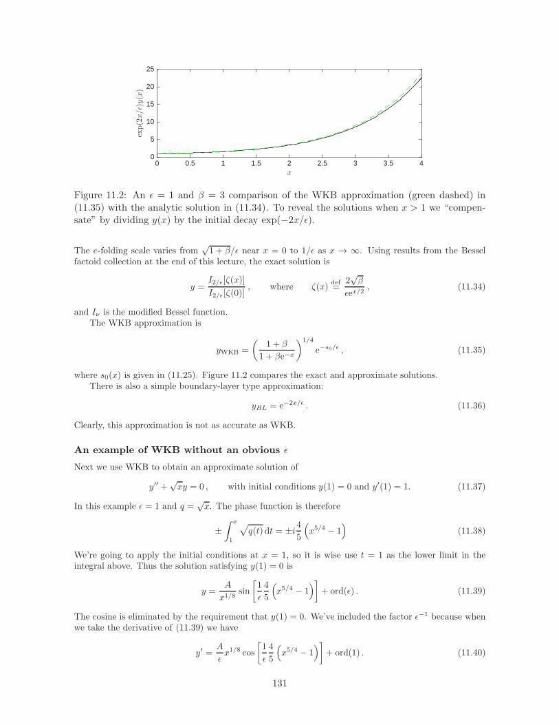
0 0.5 1 1.5 2 2.5 3 3.5 4x

0

5

10

15

20

25

exp(2x/ǫ)y(x)

Figure 11.2: An ǫ = 1 and β = 3 comparison of the WKB approximation (green dashed) in(11.35) with the analytic solution in (11.34). To reveal the solutions when x > 1 we “compen-sate” by dividing y(x) by the initial decay exp(−2x/ǫ).

The e-folding scale varies from√1 + β/ǫ near x = 0 to 1/ǫ as x → ∞. Using results from the Bessel

factoid collection at the end of this lecture, the exact solution is

y =I2/ǫ[ζ(x)]

I2/ǫ[ζ(0)], where ζ(x)

def=

2√β

ǫex/2, (11.34)

and Iν is the modified Bessel function.The WKB approximation is

yWKB =

(1 + β

1 + βe−x

)1/4

e−s0/ǫ , (11.35)

where s0(x) is given in (11.25). Figure 11.2 compares the exact and approximate solutions.There is also a simple boundary-layer type approximation:

yBL = e−2x/ǫ . (11.36)

Clearly, this approximation is not as accurate as WKB.

An example of WKB without an obvious ǫ

Next we use WKB to obtain an approximate solution of

y′′ +√xy = 0 , with initial conditions y(1) = 0 and y′(1) = 1. (11.37)

In this example ǫ = 1 and q =√x. The phase function is therefore

±∫ x

1

√

q(t) dt = ±i45

(

x5/4 − 1)

(11.38)

We’re going to apply the initial conditions at x = 1, so it is wise use t = 1 as the lower limit in theintegral above. Thus the solution satisfying y(1) = 0 is

y =A

x1/8sin

[1

ǫ

4

5

(

x5/4 − 1)]

+ ord(ǫ) . (11.39)

The cosine is eliminated by the requirement that y(1) = 0. We’ve included the factor ǫ−1 because whenwe take the derivative of (11.39) we have

y′ =A

ǫx1/8 cos

[1

ǫ

4

5

(

x5/4 − 1)]

+ ord(1) . (11.40)

131

0 5 10 15 20 25 30 35 40 45 50

x

-1

-0.5

0

0.5

1

y(x)

0 0.5 1 1.5 2 2.5 3 3.5 4 4.5 5

x

-2

-1.5

-1

-0.5

0

0.5

1

y(x)

Figure 11.3: Comparison of the WKB approximation (black dashed) in (11.41) with a matlab

integration (solid blue) of the initial value problem (11.3) (shooting both ways starting atx = 1). The upper panel shows close agreement over a large interval and the lower panel showsfailure of the WKB approximation close to the turning point at x = 0.

When we take the derivative we only differentiate the cosine and not the amplitude x−1/8 — the derivativeof the amplitude factor is order ǫ smaller. Requiring that y′(1) = 1 we see that A = ǫ = 1. Thus theWKB approximation is

yWKB(x) = x−1/8 sin

[4

5

(

x5/4 − 1)]

. (11.41)

Figure 11.3 shows that this is an excellent approximation to the solution to the initial value problem —unless we get too close to the turning point at x = 0.

Why does the WKB approximation work when there is no ǫ? Suppose we’re interested in thesolutions of (11.37) with x large. If we introduce

Xdef= δ x (11.42)

then the rescaled equation isδ5/2yXX +

√Xy = 0 . (11.43)

As δ → 0 with X fixed we obtain the standard WKB problem with the small parameter

ǫ = δ5/4 . (11.44)

Thus we expect that the PO approximation (11.41) is asymptotic as x→ ∞.Now consider the more general equation

y′′ + xay = 0 . (11.45)

Is the WKB approximation valid as x → ∞? The problems invite you to explore this issue in detaile.g., by examining the higher order corrections to the physical optics approximation. But the re-scalingargument shows very quickly that WKB is valid provided that a > −2.

Exercise: Show that as x→ ∞ the WKB approximation applies to (11.45) provided that a > −2.

132

0 5 10 15 20 25 30 35 40 45 50

x

-25

-20

-15

-10

-5

0

5

10

y,y W

KB&

y pert ode45

WKBypert1ypert2

Figure 11.4: Failure of the WKB approximation.

Failure of WKB

Considery′′ + x−3y = 0 , with ICs y(0) = 1 and y′(1) = 0 . (11.46)

Notice that the condition for the validity of PO in (11.16) is strongly violated:

∣∣∣∣∣

s′′0s′20

∣∣∣∣∣=

3x1/2

2→ ∞ , as x→ ∞. (11.47)

Ignoring this red flag, we proceed to construct the PO approximation

yWKB = x3/4 cos[

2(

1− x−1/2)]

. (11.48)

The comparison with the numerical solution in Figure 11.4 is disastrous.Instead there is a simple iterative solution starting with y0 = 1, and then proceeding with

y′′n+1 = x−3yn . (11.49)

Iterating once and twice we have

y1 = 2− 1

2x− x

2, and y2 =

9

4− x

3− 1

2lnx− 1

x+

1

12

1

x2. (11.50)

These iterative approximations compare well with the numerics in Figure 11.4.The iterative solution is based on the idea that x−3 goes to zero rather rapidly as x→ ∞, and thus

the term x−3y has a small effect on the initial condition. But eventually as x → ∞ the approximationy2 will deviate significantly from the exact solution. To see this failure of iteration we might extend theplot in Figure 11.4 to x larger than 50. Alternatively we solve (11.37) exactly....

11.3 Validity of WKB and higher order terms

In (11.16) we obtained a necessary condition for the validity of the PO approximation. In this sectionwe provide further substantiation of the conditions required for the PO approximation to work.

The solutions of the WKB hierarchy at the next two orders are

s2 = ∓∫ x q′′

8q3/2− 5

32

q′2

q5/2dt , (11.51)

is3 =1

16

q′′

q2− 5

64

q′2

q3. (11.52)

133

These formulas are equivalent to

s2 = ±1

2

∫ x

q−1/4(

q−1/4)′′

dt (11.53)

and

is3 = −1

4q−1/2

(

q−1/4)′′

. (11.54)

Let’s apply these formulas to Airy’s equation

y′′ = xy (11.55)

with x→ ∞.

Example: Considerǫ2y′′ − x−1y = 0 . (11.56)

How small must ǫ be in order for the physical optics approximation to within 5% when x ≥ 1?

Example: Considery′′ + kx−αy = 0 , y(1) = 0 , y′(1) = 1 . (11.57)

Is WKB valid as x→ ∞?

With k = 1, I found

s0 = ± 2

2− α

(

x1−α2 − 1

)

, and s1 =α

4ln x , and s2 =

α(α− 4)

16(α− 2)

(

xα2−1 − 1

)

. (11.58)

The calculation of s2 should be checked (and should do general k). But the tentative conclusion is thatWKB works if α < 2. Note α = 2 is a special case with an elementary solution.

11.4 Eigenproblems

Consider the problem of determining the eigenfrequencies of a vibrating string with non-uniform massdensity ρ(x) and uniform tension T :

φxx + ω2 ρ

T︸︷︷︸

def= σ2

φ = 0 . (11.59)

The wave speed is σ−1 — let’s follow our friend the seismologists and refer to the inverse wave speedσ as the “slowness”. The ends of the string at x = 0 and ℓ are “clamped” i.e., we have the Dirichletboundary conditions

φ(0) = φ(ℓ) = 0 . (11.60)

The eigenfrequencies are ordered0 < ω1 < ω2 < · · · (11.61)

and we know that ωn → ∞ as n→ ∞. To find an approximation to these large eigenvalues, we say thatωn = ǫ−1 and rewrite the differential equation as

ǫ2φxx + σ2φ = 0 . (11.62)

The PO approximation is then:

φPO = aσ−1/2 sin

[

ω

∫ x

0

σ(x′) dx′]

, (11.63)

where a is a normalization constant. The construction above secures the boundary condition at x = 0.The other boundary condition at x = 1 provides the eigenfrequency

ωPOn =

nπ∫ ℓ

0σ(x) dx

. (11.64)

134

1 1.5 2 2.5 3 3.5 4 4.5 5Mode Number

0

0.5

1

1.5

2

2.5

3

percenterrore

0 0.1 0.2 0.3 0.4 0.5 0.6 0.7 0.8 0.9 1

x

-1.5

-1

-0.5

0

0.5

1

1.5

y 5(x)

Figure 11.5: Upper panel shows the percentage error in (11.69). The lower panel compares thefifth eiegnfunction determined by bvp4c (the blue solid curve) with the WKB eigenfunction(the black dashed curve).

A standard way of normalizing the eigenfunctions is to require

1 =

∫ ℓ

0

φ2nσ2 dx . (11.65)

This normalization determines a in (11.63) as

1 = a2∫ ℓ

0

sin2[

ωPO

∫ x

0

σ(x′) dx′]

σ(x) dx . (11.66)

We can evaluate the integral above using the “WKB coordinate”

ξ(x)def=

∫ x

0σ(x′) dx′

∫ ℓ

0σ(x′) dx′

=ωPOn

nπ

∫ x

0

σ(x′) dx′ ⇒ σdx =

(∫ ℓ

0

σ dx

)

dξ . (11.67)

In terms of ξ, the normalization condition (11.65) is

1 = a2

(∫ ℓ

0

σ dx

)∫ 1

0

sin2 (nπξ) dξ

︸ ︷︷ ︸

=1/2

. (11.68)

Example: If σ = 1 + x2 and ℓ = 1 then (11.64) gives

ωPOn =

3πn

4. (11.69)

The upper panel of Figure 11.5 shows the percentage error

edef= 100

ω2 − (3πn/4)2

ω2, (11.70)

with ω determined numerically using bvp4c. The error is less than 3% even for the first mode.

135

0 0.5 1 1.5 2 2.5 3 3.5 4 4.5 50

5

10

15

20

Mode Numbere

1 1.5 2 2.5 3 3.5 4 4.5 5−0.5

0

0.5

x

y5(x

)

Figure 11.6: Solution with L = 5. Notice there are five interior zeros.

Example: Let’s use the WKB approximation to estimate the eigenvalues of the Sturm-Liouville eigenproblem

y′′ + λ(x+ x−1)

︸ ︷︷ ︸

w(x)

y = 0 , with BCs y′(1) = 0 , y(L) = 0 . (11.71)

The eigenvalues are function of the parameter L. The physical optics approximation is

y = w−1/4 sin(

λ1/2

∫ L

x

√

w(x′) dx′

︸ ︷︷ ︸

phase

)

, (11.72)

and the leading-order derivative is

y′ = −λ1/2w+1/4 cos

(

λ1/2

∫ L

x

√

w(x′) dx′)

. (11.73)

Notice how the phase in (11.72) has been constructed so that the boundary condition at x = L is alreadysatisfied. To apply the derivative boundary condition at x = 1 we have from (11.73)

√

λWKBn J(L) = π

(

n+1

2

)

, n = 0, 1, · · · (11.74)

where

J(L)def=

∫ L

1

√

x+ x−1 dx . (11.75)

In Figure 11.6 we take L = 5 and compare the WKB eigenvalue with those obtained from the matlab

routine bvp4c. It is not easy to analytically evaluate J(L), so instead we calculate J(L) using quad. Figure11.6 shows the relative percentage error,

e ≡ 100 × λbvp4c − λWKB

λbvp4c, (11.76)

as a function of n = 0, 2, · · · 5. The WKB approximation has about 18% error for λ0, but the highereigenvalues are accurate.

Example: Compute the next WKB correction to the n = 0 eigenvalue and compare both (11.74) and theimproved eigenvalue to the numerical solution for 1 ≤ L ≤ 10.

136

An eigenproblem with a turning point

Let’s apply the WKB approximation to estimate the large eigenvalues of the Sturm-Liouville eigenprob-lem

φ′′ + λ sinxφ = 0 , φ(0) = φ(π

2

)

= 0 . (11.77)

There is a turning point at x = 0 so the WKB approximation does not apply close to the boundary.Hope is eternal and we begin by ignoring the turning point and constructing a physical optics

approximation:

φhope = (sinx)−1/4 sin

(√λ

∫ x

0

√sin v dv

)

. (11.78)

The construction above satisfies the boundary condition at x = 0 and then the other boundary conditionat π/2 determines our hopeful approximation to the eigenvalue. To ensure that φhope(π/2) = 0, theargument of the sin must be nπ and thus the approximate eigenvalue is

λhopen =(nπ

J

)2

, n = 1 , 2 , · · · (11.79)

In the expression above the integral of the phase function is

Jdef=

∫ π/2

0

√sin v dv =

√

2

πΓ2

(3

4

)

= 1.19814 · · · (11.80)

We’ll see later that the approximation in (11.79) is not very accurate — we can’t ignore the turningpoint and hope for the best. Instead we use a combination of WKB and asymptotic matching to accountfor the turning point and obtain a better approximation to the eigenvalues.

The outer solution — use WKB: we apply the WKB approximation where it is guaranteed to work.This is in the outer region defined by λ1/3x≫ 1. The construction that satisfies the boundary conditionat x = π/2 is

φWKB = (sinx)−1/4 sin

(√λ

∫ π/2

x

√sin tdt

)

. (11.81)

To perform the match we will need the “inner limit” of the approximation above. In the region where

λ−1/3 ≪ x≪ 1 (11.82)

the WKB approximation is valid and we can simplify the phase function in (11.81):

φWKB = (sinx)−1/4 sin

(√λJ −

∫ x

0

√sin v dv

)

, (11.83)

∼ x−1/4 sin(√

λJ − 23

√λx3/2 + ord

(

x7/2))

. (11.84)

The inner solution: close to x = 0 — specifically in the region where xλ1/3 is order unity — we canapproximate the differential equation by

φxx + λ(x+ ord(x3)

)φ = 0 . (11.85)

As an inner variable we useX = λ1/3x , (11.86)

so that the leading-order inner approximation is a variant of Airy’s equation

ΦXX +XΦ = 0 . (11.87)

The solution that satisfies the boundary condition at X = 0 is

Φ = Q

[Ai(−X)

Ai(0)− Bi(−X)

Bi(0)

]

. (11.88)

137

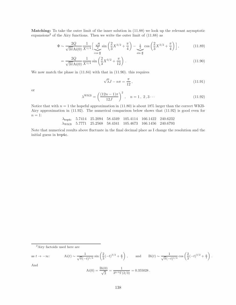
Matching: To take the outer limit of the inner solution in (11.88) we look up the relevant asymptoticexpansions2 of the Airy functions. Then we write the outer limit of (11.88) as

Φ ∼ 2Q√3πAi(0)

1

X1/4

[ √32︸︷︷︸

cos π6

sin

(2

3X3/2 +

π

4

)

− 12︸︷︷︸

sin π6

cos

(2

3X3/2 +

π

4

)]

, (11.89)

=2Q√

3πAi(0)

1

X1/4sin

(2

3X3/2 +

π

12

)

. (11.90)

We now match the phase in (11.84) with that in (11.90). this requires

√λJ − nπ =

π

12, (11.91)

or

λWKB =

((12n− 1)π

12J

)2

, n = 1 , 2 , 3 · · · (11.92)

Notice that with n = 1 the hopeful approximation in (11.80) is about 18% larger than the correct WKB-Airy approximation in (11.92). The numerical comparison below shows that (11.92) is good even forn = 1:

λbvp4c 5.7414 25.2094 58.4349 105.4114 166.1422 240.6232λWKB 5.7771 25.2568 58.4341 105.4673 166.1456 240.6793

Note that numerical results above fluctuate in the final decimal place as I change the resolution and theinitial guess in bvp4c.

2Airy factoids used here are

as t→ −∞: Ai(t) ∼ 1√π(−t)1/4 sin

(2

3(−t)3/2 + π

4

)

, and Bi(t) ∼ 1√π(−t)1/4 cos

(2

3(−t)3/2 + π

4

)

.

And

Ai(0) =Bi(0)√

3=

1

32/3Γ(2/3)= 0.355028 .

138

11.5 Using bvp4c

In this section I discuss the matlab solution of (11.71)

y′′ + λ(x+ x−1

)

︸ ︷︷ ︸

w(x)

y = 0 , with BCs y′(1) = 0 , y(L) = 0 .

To use bvp4c we let y1(x) = y(x) and write the eigenproblem as the first-order system

y′1 = y2 , (11.93)

y′2 = −λ(x+ x−1

)y1 , (11.94)

y′3 =(x+ x−1

)y21 . (11.95)

This Sturm-Liouville boundary value problem always has a trivial solution viz., y(x) = 0 and λ arbitrary.We realize that this is trivial, but perhaps bvp4c isn’t that smart. So with (11.95) we force bvp4c tolook for a nontrivial solution by adding an extra equation with the boundary conditions

y3(0) = 0 , and y3(L) = 1 . (11.96)

We also have y2(1) = 0 and y1(L) = 0, so there are four boundary conditions on a third-order problem.This is OK because we also have the unknown parameter λ. The addition of y3(x) also ensures thatbvp4c returns a normalized solution:

∫ L

1

y2(x+ x−1

)dx = 1 . (11.97)

An alternative that avoids the introduction of y3(x) is to use y1(1) = 1 as a normalization, and as anadditional boundary condition. However the normalization in (11.97) is standard.

In summary, the system for [y1, y2, y3] now only has nontrivial solutions at special values of theeigenvalue λ.

The matlab function billzWKBeig, with neither input nor output arguments, solves the eigenprob-lem with L = 5. The code is written as an argumentless function so that three nested functions can beembedded. This is particularly convenient for passing the parameter L — avoid global variables. Noticethat all functions are concluded with end. In this relatively simple application of bvp4c there are onlythree arguments:

1. a function odez that evaluates the right of (11.93) through (11.95);

2. a function bcz for evaluating the residual error in the boundary conditions;

3. a matlab structure solinit that provides a guess for the mesh and the solution on this mesh.

solinit is set-up with the utility function bvpinit, which calls the nested function initz. bvp4c

returns a matlab structure that I’ve imaginatively called sol. In this structure, sol.x contains themesh and sol.y contains the solution on that mesh. bvp4c uses the smallest number of mesh pointsit can. So, if you want to make a smooth plot of the solution, as in the lower panel of Figure 11.6,then you need the solution on a finer mesh, called xx in this example. Fortunately sol contains all theinformation needed to compute the smooth solution on the fine mesh, which is done with the auxiliaryfunction deval.

139

function billzWKBeig

L = 5; J = quad(@(x)sqrt(x+x.^(-1)),1,L);

%The first 6 eigenvalues; n = 0 is the ground state.

nEig = [0 1 2 3 4 5]; lamWKB = (nEig+0.5).^2*(pi/J)^2;

lamNum = zeros(1,length(lamWKB));

for N = 1:1:length(nEig)

lamGuess = lamWKB(N);

x = linspace(1,L,10);

solinit = bvpinit(x,@initz,lamGuess);

sol = bvp4c(@odez,@bcz,solinit);

lambda = sol.parameters;

lamNum(N) = lambda;

end

err = 100*(lamNum - lamWKB)./lamNum;

figure

subplot(2,1,1)

plot(nEig,err,’*-’)

xlabel(’Mode Number’,’interpreter’,’latex’)

ylabel(’$e$’,’interpreter’,’latex’,’fontsize’,16)

% Plot the last eigenfunction

xx = linspace(1,L); ssol = deval(sol,xx);

subplot(2,1,2)

plot(xx,ssol(1,:))

xlabel(’$x$’,’interpreter’,’latex’,’fontsize’,16)

ylabel(’$y_5(x)$’,’interpreter’,’latex’,’fontsize’,16)

%--------------- Nested Functions ----------------%

function dydx = odez(x,y,lambda)

%ODEZ evalates the derivatives

dydx = [ y(2); -lambda*(x+x^(-1))*y(1);

(x+x^(-1))*y(1)*y(1)];

end

%% BCs applied

function res = bcz(ya, yb, lambda)

res = [ ya(2) ; yb(1); ya(3) ; yb(3) - 1];

%Four BCs: solve three first-order

%equations and also determine lambda.

end

%% Use a simple guess for the Nth eigenmode

function yinit = initz(x)

alpha = (N + 1/2)*pi/(L-1);

yinit = [ sin(alpha*(L - x))

alpha*cos(alpha*(L - x))

(x - 1)/(L - 1) ];

end

end

140

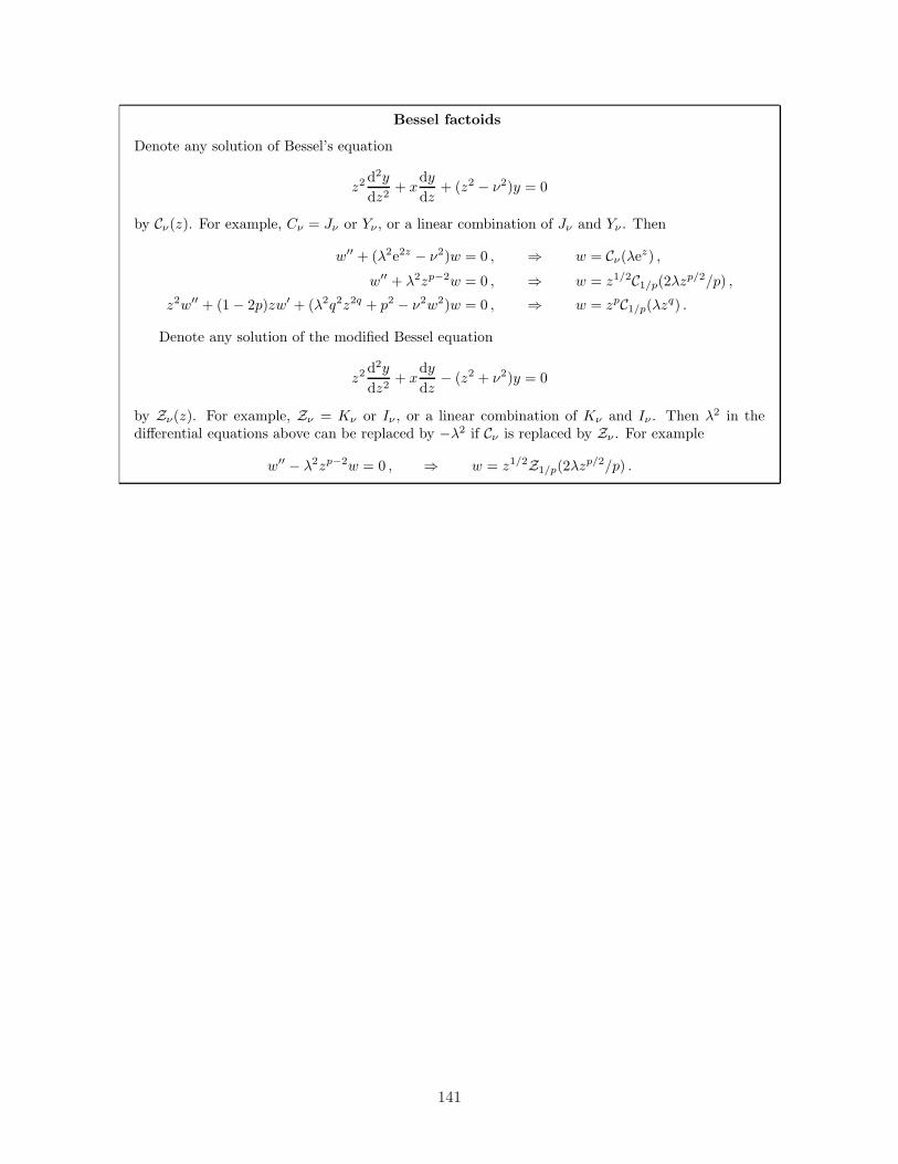
Bessel factoids

Denote any solution of Bessel’s equation

z2d2y

dz2+ x

dy

dz+ (z2 − ν2)y = 0

by Cν(z). For example, Cν = Jν or Yν , or a linear combination of Jν and Yν . Then

w′′ + (λ2e2z − ν2)w = 0 , ⇒ w = Cν(λez) ,w′′ + λ2zp−2w = 0 , ⇒ w = z1/2C1/p(2λzp/2/p) ,

z2w′′ + (1 − 2p)zw′ + (λ2q2z2q + p2 − ν2w2)w = 0 , ⇒ w = zpC1/p(λzq) .

Denote any solution of the modified Bessel equation

z2d2y

dz2+ x

dy

dz− (z2 + ν2)y = 0

by Zν(z). For example, Zν = Kν or Iν , or a linear combination of Kν and Iν . Then λ2 in thedifferential equations above can be replaced by −λ2 if Cν is replaced by Zν . For example

w′′ − λ2zp−2w = 0 , ⇒ w = z1/2Z1/p(2λzp/2/p) .

141

11.6 Problems

Problem 11.1. Consider the IVP

x+ 256e4tx = 0 , x(0) = 0 , x(0) = 1 . (11.98)

Estimate the position and magnitude of the first positive maximum of y(t). Compare the WKB approx-imation with a numerical solution on the interval 0 < t ≤ 1.

Problem 11.2. Consider the differential equation

y′′ +400

400 + x2︸ ︷︷ ︸

Q(x)

y = 0 . (11.99)

How can we apply the WKB approximation to this equation? Compare the physical optics approximationto a numerical solution with the initial conditions y(0) = 1 and y′(0) = 0.

Problem 11.3. Considery′′ +

a

x2y = 0 . (11.100)

Take a > 0 and obtain the physical-optics approximation. Compare to the exact solution. Is the physical-optics approximation asymptotically valid as x → ∞? As x → 0? Is the physical-optics approximationever valid?

Problem 11.4. Find an approximation to the large eigenvalues of the Sturm-Liouville problem

φ′′ + λe2xφ = 0 , posed on 0 < x < 1, with BCs: φ(0) = 0 , φ′(1) = 0 . (11.101)

(Bonus for comparison with a numerical solution.)

Problem 11.5. Substitute the WKB ansatz y = eS/ǫ into the fourth- order differential equation

ǫ4d4y

dx4+Qy = 0 , (11.102)

and obtain a nonlinear equation for S. Using the expansion S = S0 + ǫS1 + ǫ2S2 + · · · find S0 and S1

in terms of Q. (Consider both signs of Q.)

Problem 11.6. Put Bessel’s differential equation

r2d2y

dr2+ r

dy

dr+ (r2 − ν2)y = 0 (11.103)

into Schrodinger formd2Y

dr2+

(

1− ν2 − 14

r2

)

Y = 0 . (11.104)

Consider r = R/ǫ with ǫ→ 0 and R fixed. Obtain the physical optics approximation to (11.104) in thislimit. Compare your answer to Bessel-function asymptotics in some convenient reference.

Problem 11.7. Consider the differential equation

y′′ + x2y = 0 , with ICs y(1) = 0 , y(1) = 1 , (11.105)

posed on the semi-infinite interval x > 1. Solve the differential equation using the PO approximationand assess the accuracy of the large-x PO approximation by considering the third term in the WKBexpansion. Find the exact solution in terms of Bessel functions. Use matlab to compare the Besselfunction solution with the WKB approximation.

142

0 0.5 1 1.5 2 2.5 3-0.2

-0.1

0

0.1

0.2

0.3

Figure 11.7: A figure for problem 11.8.

Problem 11.8. The top panel of figure 11.7 shows the solution to one of the four initial value problems:

ǫ2y′′1 − e−xy1 = 0 , y1(0) = 0 , y′1(0) = 1 ,

ǫ2y′′2 − exy2 = 0 , y2(0) = 0 , y′2(0) = 1 ,

ǫ2y′′3 + e−xy3 = 0 , y3(0) = 0 , y′3(0) = 1 ,

ǫ2y′′4 + exy4 = 0 , y4(0) = 0 , y′4(0) = 1 .

(a) Which yn(x) is shown in figure 11.7? (b) Use the WKB approximation to estimate the value of ǫused in figure 11.7.

Problem 11.9. Estimate the large eigenvalues of

ψ′′ + λ sin2 xψ = 0 , with BCs y(0) = y(π/2) = 0. (11.106)

Compute the first five eigenvalues with bvp5c and compare the numerical estimate with your approxi-mation.

Problem 11.10. Use the exponential substitution y = exp(S/ǫ) to construct a WKB approximation tothe differential equation

ǫ2 (py′)′+ qy = 0 . (11.107)

Above p(x) and q(x) are coefficient functions, independent of the small parameter ǫ.

Problem 11.11. Consider the eigenproblem

φ′′ + λwφ = 0 , φ(0) = 0 , φ′(1) + φ(1) = 0 . (11.108)

The weight function, w(x) above, is positive for 0 ≤ x ≤ 1. (i) Show that the eigenvalues λn are realand positive. (ii) Show that eigenfunctions with distinct eigenvalues are orthogonal

(λn − λm)

∫ 1

0

φnφmw dx = 0 . (11.109)

(iii) With w = 1, find the first five eigenvalues and plot the first five eigenfunctions. You should obtaintranscendental equation for λ, and then solve that equation with matlab. (iv) Next, with non-constantw(x), use the WKB approximation to obtain a formula for λn. (v) Consider

w = (a+ x)2 . (11.110)

Take a = 1 and use bvp4c to calculate the first five eigenvalues and compare λWKB with λbvp4c. (vi) Isthe WKB approximation better or worse if a increases?

143

Problem 11.12. Consider the Sturm-Liouville problem

(wy′)′ + λy = 0 , (11.111)

with boundary conditionslimx→0

wy′ = 0 , y(1) = 0 . (11.112)

Assume that w(x) increases monotonically with w(0) = 0 and w(1) = 1 e.g., w(x) = sinπx/2. Further,suppose that if x≪ 1 then

w(x) = w1x+w2

2x2 +

w3

6x3 + · · · . (11.113)

There is a regular singular point at x = 0, and thus we require only that y(0) is not infinite.Show that the transformation y = w−1/2Y puts the equation into the Schrodinger form

Y ′′ +

[λ

w− w′′

2w+w′2

4w2

]

Y = 0 . (11.114)

Use the WKB method and matching to find an approximation for the large eigenvalues (λ = ǫ−2 ≫ 1)in terms of the wn’s and the constant

q ≡∫ 1

0

dx√

w(x). (11.115)

Some useful information from DLMF: The solution of

u′′ +

[a2

4z+

1− ν2

4z2

]

u = 0 (11.116)

isu(z) = A

√zJν(a

√z) +B

√zYν(a

√z) , (11.117)

where Jν and Yν are Bessel functions. You will need to look up basic properties of Bessel functions.

Problem 11.13. Consider the epsilonless Schrodinger equation

y′′ + p2y = 0 , (11.118)

where p(x) > 0. (i) Try to solve the equation by substituting

Y ≡ exp

(

±i

∫ x

0

p(t) dt

)

. (11.119)

Unfortunately this doesn’t work: Y (x) is not an exact solution of (11.118) unless p is constant. Instead,show that Y satisfies

Y ′′ +(p2 ∓ ip′

)Y = 0 . (11.120)

(ii) Compare (11.120) with (11.118), and explain why Y (x) is an approximate solution of (11.118) if

∣∣∣∣

d

dx

1

p

∣∣∣∣≪ 1 . (11.121)

(iii) Prove that if y1 and y2 are two linearly independent solutions of (11.118) then the Wronskian

W ≡ y1y′2 − y′1y2 (11.122)

is constant. (iv) Show that the Wronskian of

Y1 ≡ exp

(

+i

∫ x

0

p(t) dt

)

and Y2 ≡ exp

(

−i

∫ x

0

p(t) dt

)

(11.123)

144

−2 0 2 4 6 8 10 12

0

2

4

6

8

10

x

y(x

)

Figure 11.8: Figure for the problem 11.14 showing a comparison of the exact solution (thesolid black curve) with the asymptotic expansions as x → −∞ (the dot-dash blue curve) and(11.126) as x→ +∞ (the dashed red curve).

is equal to 2ip. This suggests that if we modify the amplitude of Y (x) like this:

Y3 ≡ 1√pexp

(

+i

∫ x

0

p(t) dt

)

and Y4 ≡ 1√pexp

(

−i

∫ x

0

p(t) dt

)

, (11.124)

then we might have a better approximation. (v) Show that the Wronskian of Y3 and Y4 is a constant.(vi) Find a Schrodinger equation satisfied by Y3 and Y4 and discuss the circumstances in which thisequation is close to (11.118).

Problem 11.14. Considery′′ + xy = 0 , (11.125)

and suppose thaty(x) ∼ x−1/4 cos(2x3/2/3) as x→ +∞ . (11.126)

Solve this problem exactly in terms of well known special functions. Find the asymptotic behaviour ofy(x) as x→ −∞. Check your answer with matlab (see Figure 11.14)

Problem 11.15. (i) Consider the eigenproblem

y′′ + E (1 + ηx) y = 0 , y(0) = 0 , y(π) = 0 , (11.127)

where η is a parameter and E is an eigenvalue. With η = 0 the gravest mode is

y = sinx , E = 1 . (11.128)

(i) Suppose |η| ≪ 1. Find the O(η) shift in the eigenvalue using perturbation theory. If you’re energetic,calculate the O(η2) term for good measure (optional). (ii) In equation (10.1.31) of BO, there is a WKBapproximation to the eigenvalue E(η). Take n = 1, and expand this formula for E up to and includingterms of order η2; compare this with your answer to part (i). (iii) Use bvp4c in MATLAB to calculateE(η), with 0 < η < 2, numerically. Compare the WKB approximation in (10.1.31) with your numericalanswer by plotting Ebvp4c(η) and EWKB(η) in the same figure.

Problem 11.16. Consider the Sturm-Liouville eigenproblem

y′′ + λ (1 + a sinx)2y = 0 , y(0) = y(π) = 0 . (11.129)

(a) Using bvp4c, compute the first two eigenvalues, λ1 and λ2, as a functions of a in the range −3/4 <a < 3. (b) Estimate λ1(a) and λ2(a) using the WKB approximation. (c) Assuming |a| ≪ 1 use

145

0 0.2 0.4 0.6 0.8 1 1.2 1.4 1.6 1.8 20.2

0.4

0.6

0.8

1

η

E

bvp4cWKB

0 0.2 0.4 0.6 0.8 1 1.2 1.4 1.6 1.8 2−5

0

5

10

η

perc

enta

ge e

rror

Figure 11.9: Figure for the problem with (11.127).

perturbation theory to compute the first two nonzero terms in the expansion of λ1(a) and λ2(a) abouta = 0. Compare these approximations with the WKB solution — do they agree? (d) Compare theWKB approximation to those from bvp4c by plotting the various results for λn(a)/n

2 on the interval−3/4 < a < 3.

Remark: If a = −1 the differential equation has a turning point at x = π/2. This requires specialanalysis — so we’re staying well away from this ticklish situation by taking a > −3/4.

146

−0.5 0 0.5 1 1.5 2 2.5 30

0.5

1

1.5

2

2.5

3

3.5

4

a

λ / n

Eig

2

Eigenvalues for y’’ + λ(1 + a sin x)2 y = 0.

First eigenvalueSecond eigenvalueWKB

Figure 11.10: Figure for the problem containing (11.129).

147

Lecture 12

Internal boundary layers

12.1 A linear example

BO section 9.6 has an extensive discussion of the boundary layer problem

y′′ + ay′ + by = 0 , (12.1)

in which a(x) has an internal zero. Suppose that we re-define the coordinate so that the domain is−1 ≤ x ≤ 1 and the boundary conditions in (7.42) are

y(−1) = p , y(+1) = q . (12.2)

Further, suppose that a(x) has a simple zero at x = 0. The differential equation

ǫy′′ +αx

1 + x2y + βy = 0 , (12.3)

is a typical example — figure 12.1 shows some bvp4c solutions.

Case 1: α > 0

Let’s consider (12.3) with α > 0 and boundary conditions

y(−1) = 1 , y(+1) = 0 . (12.4)

This example will reveal all the main features of the general case. Our earlier arguments indicate thatboundary layers not possible at either end of the domain. Thus there is a left interior solution, u(x),satisfying the boundary condition at x = −1:

y = u0 + ǫu1 + · · · (12.5)

with leading order

αx

1 + x2u0x + βu0 = 0 , ⇒ u0 = |x|−β/α exp

[

− β

2α

(x2 − 1

)]

. (12.6)

There is also a right interior solution v(x), satisfying the boundary condition at x = +1:

y = v0 + ǫv1 + · · · (12.7)

In this case, with the homogeneous x = +1 boundary conditions in (12.4), the right interior solution iszero at all orders

vn = 0 . (12.8)

148

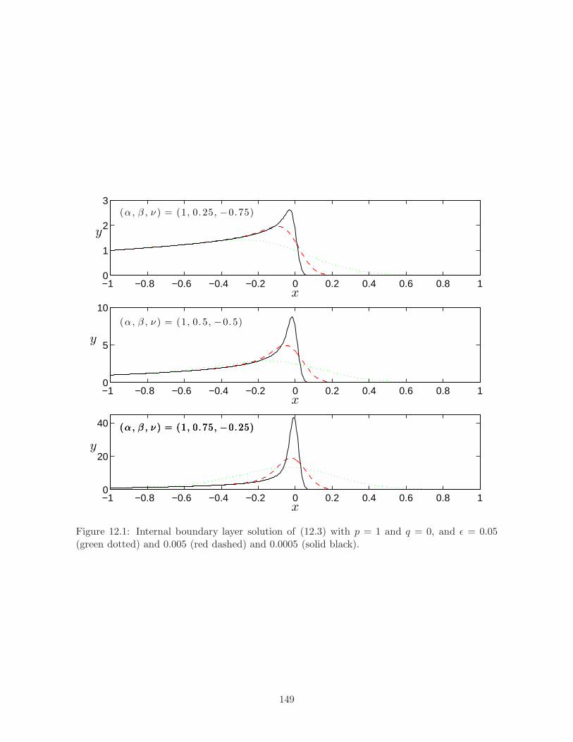
−1 −0.8 −0.6 −0.4 −0.2 0 0.2 0.4 0.6 0.8 10

1

2

3

x

y

(α , β , ν ) = (1, 0.25, −0.75)

−1 −0.8 −0.6 −0.4 −0.2 0 0.2 0.4 0.6 0.8 10

5

10

x

y

(α , β , ν ) = (1, 0.5, −0.5)

−1 −0.8 −0.6 −0.4 −0.2 0 0.2 0.4 0.6 0.8 10

20

40

x

y

(α , β , ν ) = (1, 0.75, −0.25)(α , β , ν ) = (1, 0.75, −0.25)(α , β , ν ) = (1, 0.75, −0.25)

Figure 12.1: Internal boundary layer solution of (12.3) with p = 1 and q = 0, and ǫ = 0.05(green dotted) and 0.005 (red dashed) and 0.0005 (solid black).

149

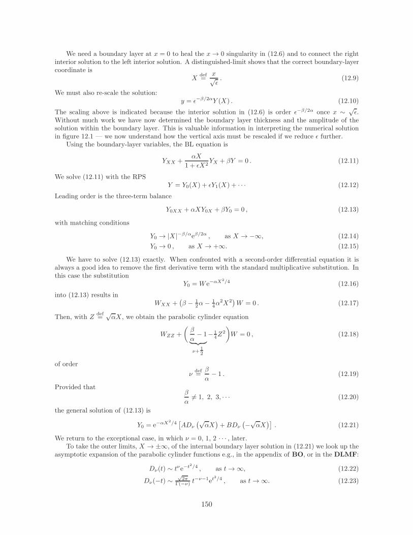
We need a boundary layer at x = 0 to heal the x→ 0 singularity in (12.6) and to connect the rightinterior solution to the left interior solution. A distinguished-limit shows that the correct boundary-layercoordinate is

Xdef=

x√ǫ. (12.9)

We must also re-scale the solution:y = ǫ−β/2αY (X) . (12.10)

The scaling above is indicated because the interior solution in (12.6) is order ǫ−β/2α once x ∼ √ǫ.

Without much work we have now determined the boundary layer thickness and the amplitude of thesolution within the boundary layer. This is valuable information in interpreting the numerical solutionin figure 12.1 — we now understand how the vertical axis must be rescaled if we reduce ǫ further.

Using the boundary-layer variables, the BL equation is

YXX +αX

1 + ǫX2YX + βY = 0 . (12.11)

We solve (12.11) with the RPSY = Y0(X) + ǫY1(X) + · · · (12.12)

Leading order is the three-term balance

Y0XX + αXY0X + βY0 = 0 , (12.13)

with matching conditions

Y0 → |X |−β/αeβ/2α , as X → −∞, (12.14)

Y0 → 0 , as X → +∞. (12.15)

We have to solve (12.13) exactly. When confronted with a second-order differential equation it isalways a good idea to remove the first derivative term with the standard multiplicative substitution. Inthis case the substitution

Y0 =W e−αX2/4 (12.16)

into (12.13) results inWXX +

(β − 1

2α− 14α

2X2)W = 0 . (12.17)

Then, with Zdef=

√αX , we obtain the parabolic cylinder equation

WZZ +

(β

α− 1

︸ ︷︷ ︸

ν+12

− 14Z

2

)

W = 0 , (12.18)

of order

νdef=

β

α− 1 . (12.19)

Provided thatβ

α6= 1, 2, 3, · · · (12.20)

the general solution of (12.13) is

Y0 = e−αX2/4[ADν

(√αX)+BDν

(−√αX)]. (12.21)

We return to the exceptional case, in which ν = 0, 1, 2 · · · , later.To take the outer limits, X → ±∞, of the internal boundary layer solution in (12.21) we look up the

asymptotic expansion of the parabolic cylinder functions e.g., in the appendix of BO, or in the DLMF:

Dν(t) ∼ tνe−t2/4 , as t→ ∞, (12.22)

Dν(−t) ∼√2π

Γ(−ν) t−ν−1et

2/4 , as t → ∞. (12.23)

150

−1 −0.8 −0.6 −0.4 −0.2 0 0.2 0.4 0.6 0.8 1−0.2

0

0.2

0.4

0.6

0.8

x

y

(α, β ) = (−1, 0.5)(α, β ) = (−1, 0.5)(α, β ) = (−1, 0.5)

0.02

(α, β ) = (−1, 0.5)

0.02

(α, β ) = (−1, 0.5)(α, β ) = (−1, 0.5)(α, β ) = (−1, 0.5)

0.1

Figure 12.2: Solutions of (12.3) with α = −1 < 0 and ǫ = 0.1 (solid blue) and 0.02 (dashedblack). There are boundary layers at x = ±1. The interior solution is zero to all orders in ǫ.There is no internal boundary layer at x = 0.

Matching in the right-hand outer limit, X → +∞, implies that B = 0. Matching in the left-handouter limit X → −∞ requires that

A = (αe)(ν+1)/2 Γ(−ν)√

2π. (12.24)

Case 2: α < 0

There is no internal boundary layer. Instead there are boundary layers at both x = 1 and x = −1. —see figure 12.2

151

Lecture 13

Initial layers

13.1 The over-damped oscillator

With our knowledge of boundary layer theory, let’s reconsider the over-damped harmonic oscillator fromproblem 4.9. With a change of notation, the problem in (4.93) is:

ǫxtt + xt + x = 0 , with the IC: x(0) = 0 , xτ (0) = 1 . (13.1)

This scaling is convenient for the long-time solution, but not for satisfying the two initial conditions.We are going to use a boundary-layer-in-time, also known as an initial layer, to solve this problem.

To address the initial layer we introduce

Tdef= t/ǫ , and X(T, ǫ) = x(t, ǫ) . (13.2)

The rescaled problem is

XTT +XT + ǫX = 0 , with the IC: X(0) = 0 , Xτ (0) = ǫ . (13.3)

Because X satisfies both the initial conditions it is convenient to attack this problem by first solving theinitial-layer equation with

X(T, ǫ) = ǫX1(T ) + ǫ2X2(T ) + · · · (13.4)

One finds

X1TT +X1T = 0 , ⇒ X1 = 1− e−T , (13.5)

X2TT +X2T = −X1 , ⇒ X1 = 2(1− e−T )− T − T e−T . (13.6)

All the constants of integration are determined because the initial-layer solution satisfies both initialconditions. Once T ≫ 1, the initial-layer solution is

X → ǫ + ǫ2 (2− T ) + ord(ǫ3) , (13.7)

= ǫ(1− t) + 2ǫ2 + ord(ǫ3) . (13.8)

We must match the outer solution onto this function — to facilitate the match, we’ve written the solutionin terms of the outer time t. Notice how the term ǫ2T switched orders. We can anticipate that thereare further switchbacks from the ord(ǫ3) terms.

We obtain the outer solution by solving (13.1) (without the initial conditions!) with the RPS

x(t, ǫ) = ǫx1(t) + ǫ2x2(t) + · · · (13.9)

The first two terms are

x1t + x1 = 0 , ⇒ x1 = A1e−t , (13.10)

x2t + x2 = −x1tt , ⇒ x1 = A1te−t +A2e

−t , (13.11)

152

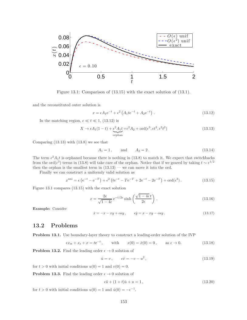
0 0.5 1 1.5 20

0.02

0.04

0.06

0.08

t

x(t)

ǫ = 0.10

O (ǫ) unifO (ǫ2) unifexact

Figure 13.1: Comparison of (13.15) with the exact solution of (13.1).

and the reconstituted outer solution is

x = ǫA1e−t + ǫ2

(A1te

−t +A2e−t). (13.12)

In the matching region, ǫ≪ t≪ 1, (13.12) is

X → ǫA1(1− t) + ǫ2A1t︸ ︷︷ ︸

orphan

+ǫ2A2 + ord(ǫ3, ǫt2, ǫ2t2) (13.13)

Comparing (13.13) with (13.8) we see that

A1 = 1 , and A2 = 2 . (13.14)

The term ǫ2A1t is orphaned because there is nothing in (13.8) to match it. We expect that switchbacksfrom the ord(ǫ3) terms in (13.8) will take care of the orphan. Notice that if we geared by taking t ∼ ǫ1/2

then the orphan is the smallest term in (13.13) — we can move it into the ord.Finally we can construct a uniformly valid solution as

xuni = ǫ(e−t − e−T

)+ ǫ2

(te−t − T e−T + 2e−t − 2e−T

)+ ord(ǫ3) . (13.15)

Figure 13.1 compares (13.15) with the exact solution

x =2ǫ√1− 4ǫ

e−t/2ǫ sinh

(√1− 4ǫ t

2ǫ

)

. (13.16)

Example: Considerx = −x− xy + ǫκy , ǫy = x− xy − ǫκy . (13.17)

13.2 Problems

Problem 13.1. Use boundary-layer theory to construct a leading-order solution of the IVP

ǫxtt + xt + x = te−t , with x(0) = x(0) = 0 , as ǫ→ 0. (13.18)

Problem 13.2. Find the leading order ǫ→ 0 solution of

u = v , ǫv = −v − u2 , (13.19)

for t > 0 with initial conditions u(0) = 1 and v(0) = 0.

Problem 13.3. Find the leading order ǫ→ 0 solution of

ǫu+ (1 + t)u+ u = 1 , (13.20)

for t > 0 with initial conditions u(0) = 1 and u(0) = −ǫ−1.

153

Problem 13.4. A function y(t, x) satisfies the integro-differential equation

ǫyt = −y + f(t) + Y (t) , (13.21)

where

Y (t)def=

∫ ∞

0

y(t, x)e−βx dx , (13.22)

with β > 1. The initial condition is y(0, x) = a(x). (This is the Grodsky model for insulin release.)Use boundary layer theory to find the composite solution on the interval 0 < t < ∞. Compare thisapproximate solution with the exact solution of the model. To assist communication, use the notation

αdef= 1− β−1 and A

def= Y (0) , and τ

def=

t

ǫ. (13.23)

Problem 13.5. Solve the previous problem with β = 1.

Problem 13.6. The Michaelis-Menten model for an enzyme catalyzed reaction is

s = −s+ (s+ k − 1)c , ǫc = s− (s+ k)c , (13.24)

where s(t) is the concentration of the substrate and c(t) is the concentration of the catalyst. The initialconditions are

s(0) = 1 , c(0) = 0 . (13.25)

Find the first term in the: (i) outer solution; (ii) the “initial layer” (τdef= t/ǫ); (iii) the composite

expansion.

154

Lecture 14

Boundary layers in fourth-order

problems

14.1 A fourth-order differential equation

Let us consider a fourth-order boundary value problem which is similar to problems occurring in thetheory of elasticity:

− ǫ2uxxxx + uxx = 1 , (14.1)

with boundary conditionsu(−1) = u′(−1) = u(1) = u′(1) = 0 . (14.2)

The outer solution might be obtained with the RPS such as

u(x, ǫ) = u0(x) + ǫ?u1(x) + · · · (14.3)

At leading order

u0xx = 1 , ⇒ u0 =x2 − 1

2. (14.4)

We’ve applied only two of the four boundary conditions above.Before worrying about higher order terms in (14.3), let’s turn to the boundary layer at x = −1. We

assume that the solution is an even function of x so the boundary layer at x = +1 can be constructedby symmetry.

If we look for a dominant balance with X = (x + 1)/δ we find that δ = ǫ. Thus we consider aboundary layer rescaling

u(x, ǫ) = U (X, ǫ) , where Xdef=

x+ 1

ǫ. (14.5)

The boundary layer problem is then

− UXXXX + UXX = ǫ2 . (14.6)

Writing the leading-order outer solution in (14.4) in terms of X , we have

u0(x, ǫ) = −ǫX +1

2ǫ2X2 . (14.7)

Anticipating that we’ll ultimately need to match the term −ǫX in (14.7), we pose the boundary-layerexpansion

U(X, ǫ) = ǫU1(X) + ǫ2U2(X) + ǫ3U3(X) + · · · (14.8)

There is no term U0(X) because the outer solution is ord(ǫ) in the matching region.

155

Thus we have the hierarchy

−U1XXXX + U1XX = 0 , (14.9)

−U2XXXX + U2XX = 1 , (14.10)

−U3XXXX + U3XX = 0 , (14.11)

and so on.The general solution of (14.9) is

U1 = A1 +B1X + C1e−X + D1

︸︷︷︸

=0

eX . (14.12)

Above we’ve anticipated that D0 = 0 to remove the exponentially growing solution. Then applying theboundary conditions at X = 0 we find

U1 = A1

(1−X − e−X

). (14.13)

To match (14.13) against the term −ǫX in the interior solution in (14.7) we take

A1 = 1 . (14.14)

Now we can construct a leading-order solution that is uniformly valid in the region near x = −1:

uuni(x) =x2 − 1

2+ ǫ(

1− e−(x+1)/ǫ)

. (14.15)

The derivative isuunix(x) = x+ e−(x+1)/ǫ , (14.16)

which is indeed zero at x = −1.

Higher order terms

The equation for U2, (14.10), has a solution

U2(X) =X2

2+A2

(1−X − e−X

). (14.17)

Above, we’ve satisfied both boundary conditions at X = 0. We’ve also matched the term ǫ2X2/2 in(14.7). To summarize, our boundary layer solution is

U(X) = ǫ(

1︸︷︷︸

orphan

−X − e−X)

+ ǫ2X2

2+ ǫ2A2

(1−X − e−X

)+ ord(ǫ3) . (14.18)

But we have unfinished business: we have not matched the orphan above with any term in the leading-order outer solution u0(x).

To take care of the orphan we must go to next order in the interior expansion:

u(x, ǫ) =x2 − 1

2+ ǫu1(x) + ord

(ǫ2). (14.19)

Thusu1xx = 0 , ⇒ u1(x) = P1

︸︷︷︸

=1

+ Q1︸︷︷︸

=0

x (14.20)

We take Q1 = 0 because the solution is even, and P1 = 1 to take care of the orphan. The solution u1(x)does not satisfy any of the four boundary conditions. To summarize, the outer solution is

u(x, ǫ) =x2 − 1

2+ ǫ+ ord(ǫ2) . (14.21)

156

The ord(ǫ) term above was accidently included in the uniform solution (14.16): in the outer region theexpansion of (14.15) already agrees with all terms in (14.21).

Because u0xxxx = 0, there are now no more non-zero terms in the outer region i.e., u2 = 0, andtherefore A2 = 0 in (14.18). Moreover, all terms U3, U4 etcetera are also zero. Thus we have constructedan infinite-order asymptotic expansion. Using symmetry we can construct a uniformly valid solutionthroughout the whole domain

uuni(x) =x2 − 1

2+ ǫ(

1− e−(x+1)/ǫ − e(x−1)/ǫ)

. (14.22)

14.2 Problems

Problem 14.1. Solve (14.1) exactly and use matlab to compare the exact solution with the asymptoticsolution in (14.22).

Problem 14.2. Find two terms in ǫ in the outer region and match to the inner solution at bothboundaries for

ǫ2u′′′′ − u′′ = eax . (14.23)

The domain is −1 ≤ x ≤ 1 with BCs

u(−1) = u′(−1) = 0 , and u(1) = u′(1) = 0 . (14.24)

Problem 14.3. Find two terms in ǫ in the outer region and match to the inner solution at bothboundaries for

ǫ2u′′′′ − u′′ = 0 . (14.25)

The domain is 0 ≤ x ≤ 1 with BCs

u(0) = 0 , u′(0) = 1 , and u(1) = u′(1) = 0 . (14.26)

Problem 14.4. Considering the eigenproblem

− ǫ2u′′′′ + u′′ = λu , (14.27)

on the domain is 0 ≤ x ≤ π with BCs

u(0) = u′(0) = 0 , and u(π) = u′(π) = 0 . (14.28)

(i) Prove that all eigenvalues are real and positive. (ii) Show that with a suitable definition of innerproduct, that eigenfunctions with different eigenvalues are orthogonal. (iii) Use boundary layer theoryto find the shift in the unperturbed spectrum, λ = 1, 2, 3 · · · , induced by ǫ.

157