PART VI. EXPERIMENTAL VERIFICATION OF PREVIOUSLY … · TECHNIQUE WITH APPLICATION TO PBI MATATIAHU...
47
AFML-TR-67-121 OFFICIAL FW-LE COPy Part Vl AvA q ý-36 7 S EVALUATION OF MOLECULAR WEIGHT FROM EQUILIBRIUM SEDIMENTATION PART VI. EXPERIMENTAL VERIFICATION OF PREVIOUSLY PROPOSED REGULARIZATION-LINEAR PROGRAMMING TECHNIQUE WITH APPLICATION TO PBI MATATIAHU T. GEHATIA DONALD R. WIFF TECHNICAL REPORT AFML-TR-67-121, PART VI NOVEMBER 1971 Approved for public release; distribution unlimited. Best Available Copy AR FORCE MATERIALS LABORATORY AIR FORCE SYSTEMS COMMAND WRIGHT-PATTERSON AIR FORCE BASE, OHIO godq O 3/1057
Transcript of PART VI. EXPERIMENTAL VERIFICATION OF PREVIOUSLY … · TECHNIQUE WITH APPLICATION TO PBI MATATIAHU...

AFML-TR-67-121 OFFICIAL FW-LE COPyPart Vl
AvA q ý-36 7 S
EVALUATION OF MOLECULAR WEIGHT
FROM EQUILIBRIUM SEDIMENTATION
PART VI. EXPERIMENTAL VERIFICATION OF PREVIOUSLY
PROPOSED REGULARIZATION-LINEAR PROGRAMMING
TECHNIQUE WITH APPLICATION TO PBI
MATATIAHU T. GEHATIA
DONALD R. WIFF
TECHNICAL REPORT AFML-TR-67-121, PART VI
NOVEMBER 1971
Approved for public release; distribution unlimited.Best Available Copy
AR FORCE MATERIALS LABORATORYAIR FORCE SYSTEMS COMMAND
WRIGHT-PATTERSON AIR FORCE BASE, OHIO
godq O 3/1057

NOTICE
When Government drawings, specifications, or other data are used for any purpose
other than in connection with a definitely related Government procurement operation,the United States Government thereby incurs no responsibility nor any obligation
whatsoever; and the fact that the government may have formulated, furnished, or in
any way supplied the said drawings, specifications, or other data, is not to be regarded
by Implication or otherwise as in any manner licensing the holder, or any other person
or corporation, or conveying any rights or permission to manufacture, use, or sell any
patented invention that may In any way be related thereto.
Copies of this report should not be returned unless return is required by securityconsiderations, contractual obligations, or notice on a specific document.
AIR FORCE: 10-1-72/100
AFML-TR-67-121
Part VI
EVALUATION OF MOLECULAR WEIGHTFROM EQUILIBRIUM SEDIMENTATION
PART VI. EXPERIMENTAL VERIFICATION OF PREVIOUSLY
PROPOSED REGULARIZATION-LINEAR PROGRAMMING
TECHNIQUE WITH APPLICATION TO PBI
MATATIAHU T. GEHATIA
DONALD R. WIFF
Approved for public release; distribution unlimited.
AFML-TR-67-121Part VI
FOREWORD
This report was prepared by the Polymer Branch of the Nonmetallic
Materials Division. The work was initiated under Project 7342, "Funda-
mental Research on Macromolecular Materials and Lubrication Phenomena,"
Task 734203, "Fundamental Principles Determining the Behavior of Macro-
molecules," with Dr. M. T. Gehatia (AFML/LNP) Project Scientist. The
work was administered by the Air Force Materials Laboratory, Wright-
Patterson Air Force Base, Ohio.
The report covers research conducted from December 1970 to May 1971,
and was submitted by the authors in May 1971.
This technical report has been reviewed and is approved.
R. L. VAN DEUSENChief, Polymer BranchNonmetallic Materials DivisionAir Force Materials Laboratory
ii

AFML-TR-67-121Part VI
ABSTRACT
The relationships between the molecular weight distribution (MWD) of
polymer in solution and concentrations (or concentration gradients)
measured under conditions of ultracentrifugal equilibrium sedimentation
can be expressed by the theory-oriented Fujita Equations. These equations,
however, frequently constitute an "Improperly Posed Problem" in the
Hadamard sense and, therefore, many attempts to infer MWD directly have
failed by giving rise to unstable and unreliable solutions.
To combat this problem, new computation-oriented expressions have
been developed in the Air Force Materials Laboratory. The new proposed
method makes possible the MWD determination of a polymer from a single
equilibrium sedimentation experiment. The authors have presented
theoretical proof of the validity of this technique in a previous report,
and here supporting experimental verification is provided. This was
accomplished by investigating narrow linear polystyrene fractions to
determine the MWD, and then by investigating MWD of a new sample created
by combining these fractions. The results obtained by applying the
newly developed method was in very good agreement with the MWD values
known a priori. Thus, the theoretical as well as the experimental
investigation successfully demonstrate the reliability of MWD deter-
mination by applying the new method.
This technique was then applied to data obtained for PBI in DMAC.
The results show that an unusually large part of this polymer is of very
low molecular weight. Follow-up to determine what effect this low
molecular weight will have upon the use properties of PBI is planned.
iii

AFML-TR-67-121Part VI
TABLE OF CONTENTS
SECTION PAGE
I INTRODUCTION 1
II EXPERIMENTAL 5
III PROCESSING VELOCITY DATA 8
1. Sedimentation Constant (S) 8
2. Diffusion Constant (D) 8
3. Determination of Experimental Parameters 9
IV PROCESSING EQUILIBRIUM SEDIMENTATION DATA 12
1. Standard Method for Homogeneous Fractions 12
2. Regularization Method for MWD Determination 12
V RESULTS 13
VI APPLICATION OF THE NEW METHOD FOR MWD DETERMINATIONOF PBI 16
VII CONCLUSIONS 17
REFERENCES 20
v
AFML-TR-67-121Part VI
ILLUSTRATIONS
FIGURE PAGE
1. Molecular Weight Distribution for Sample A UsingO<m!51O0,O00, and Am=2381; ff(m)dm=0.569 22
2. Molecular Weight Distribution for Sample B Using15,0005<m<100,000, and Am=2024; ff(m)dm=0.341 23
3. Molecular Weight Distribution for Sample C UsinglOo,Ooo0_m<18o,Ooo,and Am=1910; ff(m)dm=0.090 24
4. Molecular Weight Distribution for Sample P (Am=5120)With a Superposition of the Molecular Weight Distributionsfor Samples A, B, and C (Lm=4286). In this case ff (m)dm=
frA(m) + fB(m) + fc(m)]dm = 1. p 25
5. Molecular Weight Distribution of PBI (Purified and Dried)in DMAC at 4 0°C With the Distribution Normalized to Unity 26
vi

AFML-TR-67-121
Part VI
TABLES
TABLE PAGE
I The Investigated Fractions 5
II Preparation of the Sample P (Polydisperse) 6
III The Conducted Experiments 6
IV Velocity Sedimentation Data for Sample A 27
V Equilibrium Sedimentation Data for Sample A 28
VI Velocity Sedimentation Data for Sample B 29
VII Equilibrium Sedimentation Data for Sample B 30
VIII Velocity Sedimentation Data for Sample C 31
IX Equilibrium Sedimentation Data for Sample C 32
X Comparison of Weight Average Molecular Weights 33
XI Equilibrium Sedimentation Data and Molecular WeightDistribution for Sample P 34
XII Molecular Weight Distribution of Samples A, B, and C 35
XIII Equilibrium Sedimentation Data and Molecular WeightDistribution for PBI-MPD 36
XIV Various Moments and Ratios of Moments Computed forPBI-MPD 37
vii

AFML-TR-67-121
Part VI
SECTION I
INTRODUCTION
In our previous works (References I through 4) a method was developed
which makes it possible to determine a molecular weight distribution
(MWD) from equilibrium sedimentation. Fujita developed formulas which
express the MWD in the form of a function f(m) in the following way:
mm"x -Xmrn
or )A ]me f(m) dm, M
or
mmax : -XmC
I dc(C) [X 2 mZe Jf(m) dmo de 0 , e- Xm M (2)
where
m = the molecular weight
X = a constant determined from the experiment
- =(r2 - r2)/(r2 - r2)
r = distance from the center of rotation
ra = value of r at the meniscus
rb = value of r at the bottom
c = concentration at
c = initial concentration0

AFML-TR-67-121
Part VI
Equations I and 2 are special cases of Fredholm Integral Equations of
the First Kind:
mmox
u ( K(Cm)f(m)dm. (3)
It has been shown that Fredholm Integral Equations of the First Kind
frequently are Improperly Posed Problems (IPP) in the Hadamard sense
(References 5 and 6). Also the Fujita Equations are IPPs and their
inverse operations are unstable because to very small deviations of u()
may correspond uncontrollably large changes in f(m). Therefore, any
direct approach to evaluate f(m) as an inverse operation of Equations 1
or 2 may lead to erratically oscillating curves. Such a trial has been
done in our previous reports (References 7 and 8). A function f(m) has
been arbitrarily assumed. By applying standard experimental conditions
the functions u(C) and K(C,m) have been computed. Using these functions
a distribution function f(m) has been calculated from an inverse operation.
The so obtained f(m) fluctuated erratically and had nothing in common
with the original f(m) function.
It has been theoretically proved that an approximate determination
of MWD is possible by applying Tikhonov's regularization method
(References 1 and 3). In such a case the Fredholm Integral Equation
(Fujita Equations) will be modified in the following way:
mmax (4)
b~m W JF(m,x)f(x)dx-A"0
2

AFML-TR-67-121Part VI
Here !b(m) = JK (•,,m)u ((J)d, (5)
0
F (m, x) f •K (•m) K (C,.x) dC (6)0
and
d d4 f(m) d f(m) (7)dmi4 -a 3 dm
where 0 2 anda3 are numerical parameters. These parameters (sometimes
only one of them) are chosen with the aid of a high speed digital computer
in such a way that a • (•) function calculated from the d~termined f(m)
function will be as close as possible to the original u(6) function, or
that the norm
1' o( '-0 u (()I• ] ,dC• u(C') ,
is a minimum.
The technique of approximation replaces the integration in Equation 4
by a summation of discrete {fk} values. For different {mn} there will
be a set of linear equations. The inverse matrix of this set will
determine all values of a {fk} vector. The term A acts as a damping
factor which reduces the oscillations, i.e., stabilizes the inverse
operation.
AFML-TR-67-121
Part VI
With the help of Equation 4 very good results were obtained in case of
an arbitrarily assumed symmetrical unimodal and symmetrical bimodal f(m).
In case of an assymetrical bimodal and symmetrical trimodal distribution
good results have been obtained after incorporating linear programing
into Equation 4 (References 2 and 4).
As mentioned above, the proof of this method has been carried out
only in a theoretical manner by the arbitrary choice of the function f(m).
No experimental proof had been given, and therefore this method had not
yet been fully checked under real experimental conditions. Therefore,
the objective of the present work is to close this gap by creating an
"a priori" known distribution and by determining it with the aid of
Equation 4. This proof has been done by investigating linear polystyrene
in cyclohexane at 35.OOC (the(B)temperature).
4
AFML-TR-67-121Part VI
SECTION II
EXPERIMENTAL
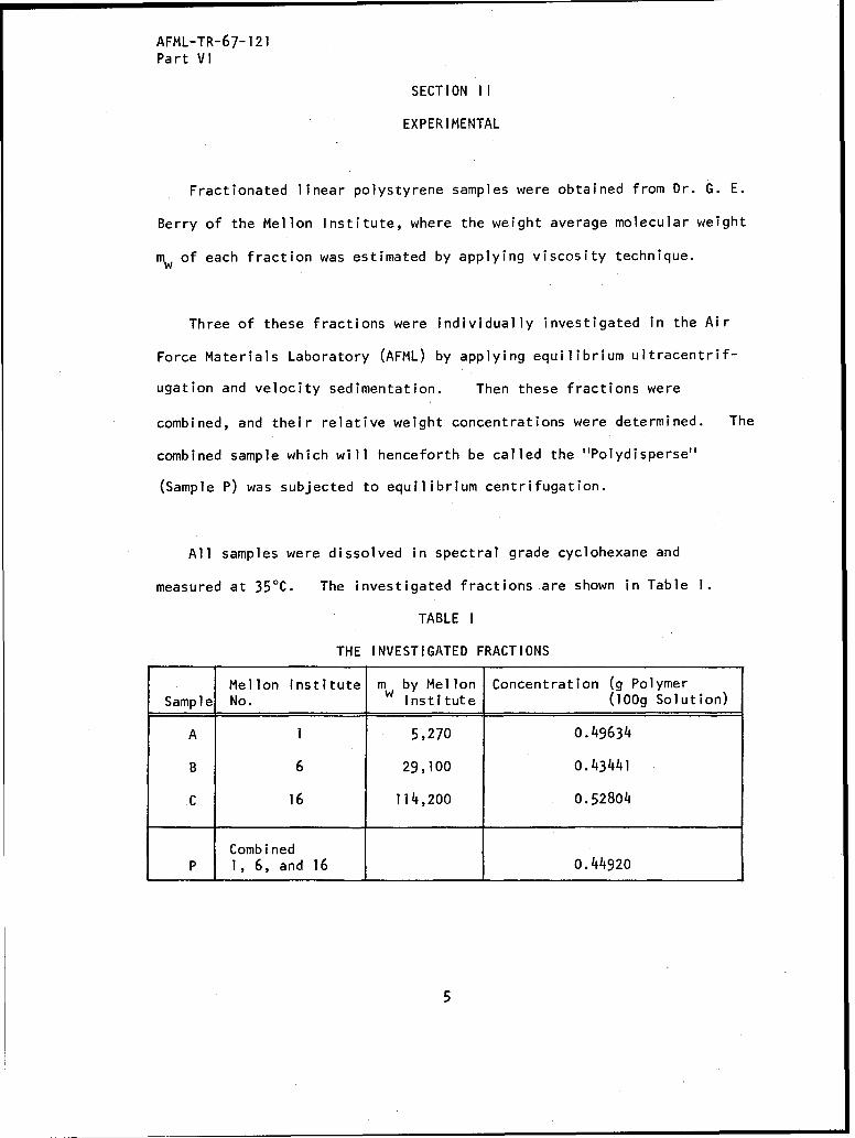
Fractionated linear polystyrene samples were obtained from Dr. G. E.
Berry of the Mellon Institute, where the weight average molecular weight
mw of each fraction was estimated by applying viscosity technique.
Three of these fractions were individually investigated in the Air
Force Materials Laboratory (AFML) by applying equilibrium ultracentrif-
ugation and velocity sedimentation. Then these fractions were
combined, and their relative weight concentrations were determined. The
combined sample which will henceforth be called the "Polydisperse"
(Sample P) was subjected to equilibrium centrifugation.
All samples were dissolved in spectral grade cyclohexane and
measured at 35'C. The investigated fractions are shown in Table 1.
TABLE I
THE INVESTIGATED FRACTIONS
Mellon Institute mw by Mellon Concentration (g PolymerSample No. Institute (1Og Solution)
A 1 5,270 0.49634
B 6 29,100 0.43441
C 16 114,200 0.52804
CombinedP 1, 6, and 16 0.44920
5
AFML-TR-67-121
Part VI
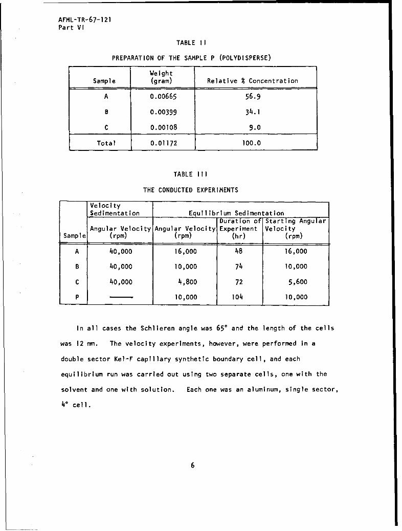
TABLE II
PREPARATION OF THE SAMPLE P (POLYDISPERSE)
WeightSample (gram) Relative % Concentration
A 0.00665 56.9
B 0.00399 34.1
C 0.00108 9.0
Total 0.01172 100.0
TABLE III
THE CONDUCTED EXPERIMENTS
VelocitySedimentation Equilibrium Sedimentation
Duration of Starting AngularAngular Velocity Angular Velocity Experiment Velocity
Sample (rpm) (rpm) (hr) (rpm)
A 40,000 16,000 48 16,000
B 40,000 10,000 74 10,000
C 40,000 4,800 72 5,600
P 10,000 104 10,000
In all cases the Schlieren angle was 650 and the length of the cells
was 12 mm. The velocity experiments, however, were performed in a
double sector Kel-F capillary synthetic boundary cell, and each
equilibrium run was carried out using two separate cells, one with the
solvent and one with solution. Each one was an aluminum, single sector,
40 cell.
6
AFML-TR-67-121
Part VI
The photographic plates obtained from each equilibrium experiment
were processed and evaluated before the experiment was terminated. Only
after such an equilibrium plot was reproducible, was the experiment
terminated.
7
AFML-TR-67-121
Part VI
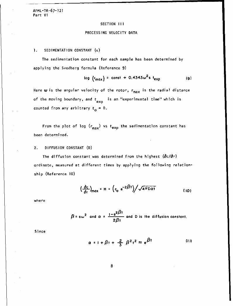
SECTION III
PROCESSING VELOCITY DATA
1. SEDIMENTATION CONSTANT (s)
The sedimentation constant for each sample has been determined by
applying the Svedberg formula (Reference 9)
log (rmax) = const + 0.4343w 2 s texp (9)
Here w is the angular velocity of the rotor, rmax is the radial distance
of the moving boundary, and t is an "experimental time" which isexp
counted from any arbitrary to 0.
From the plot of log (rmax) vs texp the sedimentation constant has
been determined.
2. DIFFUSION CONSTANT (D)
The diffusion constant was determined from the highest (ac/ir)
ordinate, measured at different times by applying the following relation-
ship (Reference 10)
ac_) c e-Z19't-/4_/7rat-r H (( (I0)
where
2 a d-e2 tsw and a and D is the diffusion constant.
2fpt
Since
at+ 2. 6 2 t 2 eot (II)
8
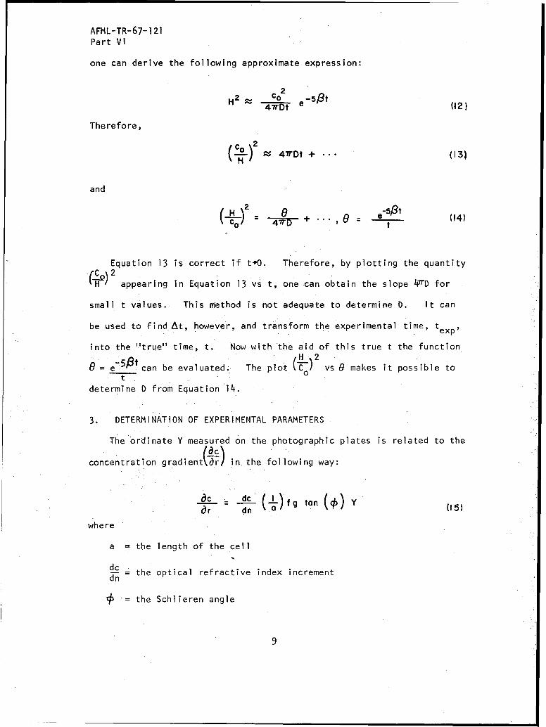
AFML-TR-67-121Part VI
one can derive the following approximate expression:
H2 ,-. C2 -5,8t"2 C0 e (12)
Therefore,
( _)2 t: ,D + .. (13)
and
0 e5 ~ (14)0 47T " t
Equation 13 is correct if t.O. Therefore, by plotting the quantityappearing in Equation 13 vs t, one can obtain the slope 47rD for
small t values. This method is not adequate to determine D. It can
be used to find At, however, and transform the experimental time, texp,
into the "true" time, t. Now with the aid of this true t the function
0 e-.5et can be evaluated. The plot C 0 vs 0 makes it possible to
* t.
determine D from Equation 14.
3. DETERMINATION OF EXPERIMENTAL PARAMETERS
The ordinate Y measured on the photographic plates is related to thea8c
concentration gradient\Wr) in the following way:
ac dc (-")fg tan ()Y (15)ar dn (05
where
a = the length of the cell
dc = the optical refractive index incrementdn
= the Schlieren angle
9
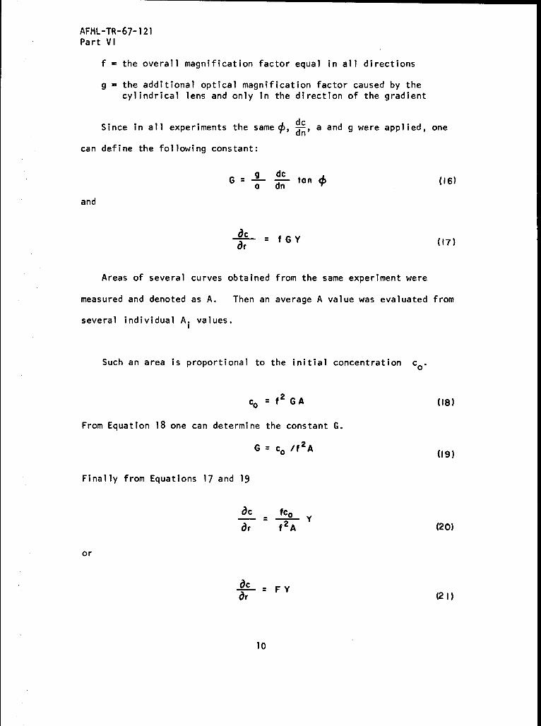
AFML-TR-67-121
Part VI
f = the overall magnification factor equal in all directions
g = the additional optical magnification factor caused by thecylindrical lens and only in the direction of the gradient
Since in all experiments the same , dc a and g were applied, one
can define the following constant:
G = g dc tona dn
and
ar f G Y
Areas of several curves obtained from the same experiment were
measured and denoted as A. Then an average A value was evaluated from
several individual A. values.I
Such an area is proportional to the initial concentration co.
Co 0 f2 GA (18)
From Equation 18 one can determine the constant G.
G co /f 2 A (19)
Finally from Equations 17 and 19
ac - fco
6r f2A (20)
or
ar (21)
10
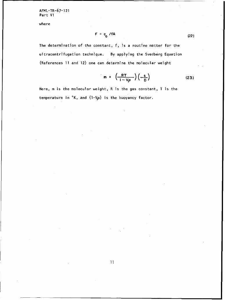
AFML-TR-67-121Part VI
where
F = c /fA (22)
The determination of the constant, f, is a routine matter for the
ultracentrifugation technique. By applying the Svedberg Equation
(References 11 and 12) one can determine the molecular weight
Here, m is the molecular weight, R is the gas constant, T is the
temperature in *K, and (1-Vp) is the buoyancy factor.
1I
AFML-TR-67- 121
Part VI
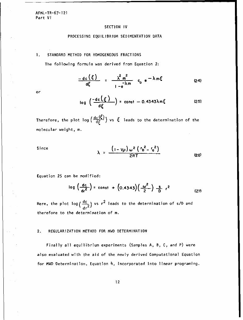
SECTION IV
PROCESSING EQUILIBRIUM SEDIMENTATION DATA
1. STANDARD METHOD FOR HOMOGENEOUS FRACTIONS
The following formula was derived from Equation 2:
22-dc(•) - X~m O*-Xm• 24- -di cM Co •-M (24)
dC I -e
or
log (-C const - O.4343XmC (25)
Therefore, the plot log (d-•-)) vs C leads to the determination of the
molecular weight, m.
Since X (I Vp) W2 (rb 2 _ ro2 )2RT (26)
Equation 25 can be modified:
log ( dc const +(0.4343) ) 2
= 2 D r(27)
Here, the plot log(dAS vs r2 leads to the determination of s/D anddr
therefore to the determination of m.
2. REGULARIZATION METHOD FOR MWD DETERMINATION
Finally all equilibrium experiments (Samples A, B, C, and P) were
also evaluated with the aid of the newly derived Computational Equation
for MWD Determination, Equation 4, incorporated into linear programing.
12
AFML-TR-67-121
Part VI
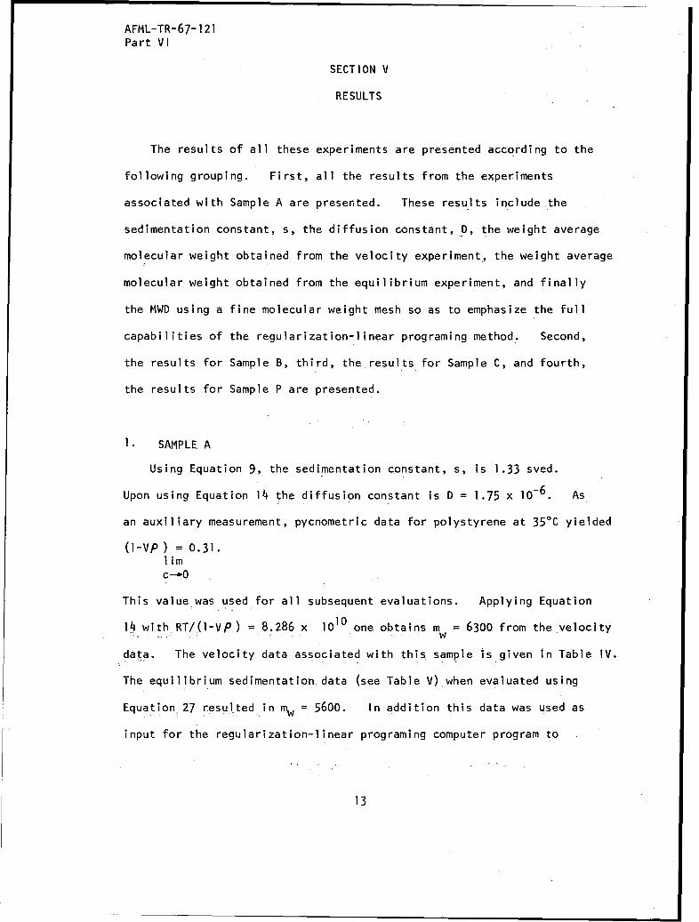
SECTION V
RESULTS
The results of all these experiments are presented according to the
following grouping. First, all the results from the experiments
associated with Sample A are presented. These results include the
sedimentation constant, s, the diffusion constant, D, the weight average
molecular weight obtained from the velocity experiment, the weight average
molecular weight obtained from the equilibrium experiment, and finally
the MWD using a fine molecular weight mesh so as to emphasize the full
capabilities of the regularization-linear programing method. Second,
the results for Sample B, third, theresults for Sample C, and fourth,
the results for Sample P are presented.
1. SAMPLE A
Using Equation 9, the sedimentation constant, s, is 1.33 sved.
Upon using Equation 14 the diffusion constant is D = 1.75 x 10⁻⁶. As
an auxiliary measurement, pycnometric data for polystyrene at 35%C yielded
(1-Vp) = 0.31.limC--.O
This value was used for all subsequent evaluations. Applying Equation
14 withRT/(l-VP) = 8.286 x 10¹⁰ one obtains m = 6300 from the velocity
data. The velocity data associated with this sample is given in Table IV.
The equilibrium sedimentation data (see Table V) when evaluated using
Equation 27 resulted in mw= 5600. In addition this data was used as
input for the regularization-linear programing computer program to
13

AFML-TR-67-121
Part VI
determine the MWD. For 05m!5100,000 the MWD for Sample A is given in
Figure 1 with ff(m)dm = 0.569.
2. SAMPLE B
Following the same procedure as that given above, s = 2.73 sved,
D = 5.50 x 10⁻⁷ (for data see Table VI), m velocity = 41,000, mw w
equilibrium = 36,700 (for data see Table VII) ahd the MWD with 15,000 :
m:l00,000 is given in Figure 2 with ff(m)dm = 0.341.
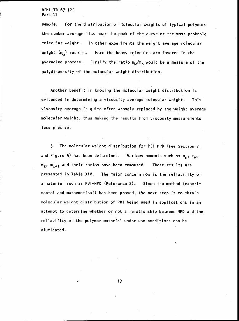
3. SAMPLE C
Again following the procedure outlined for Sample A, s = 4.97 sved,
D = 3.16 x l107 (for data see Table VIII), m velocity = 130,700, mw w
equilibrium = 146,500 (for data see Table IX), and the MWD with.l00,00O:
m:580,000 is given in Figure 3 with ff(m)dm = 0.09.
For comparison, the molecular weights of the above three samples
determined by various methods are given in Table X.
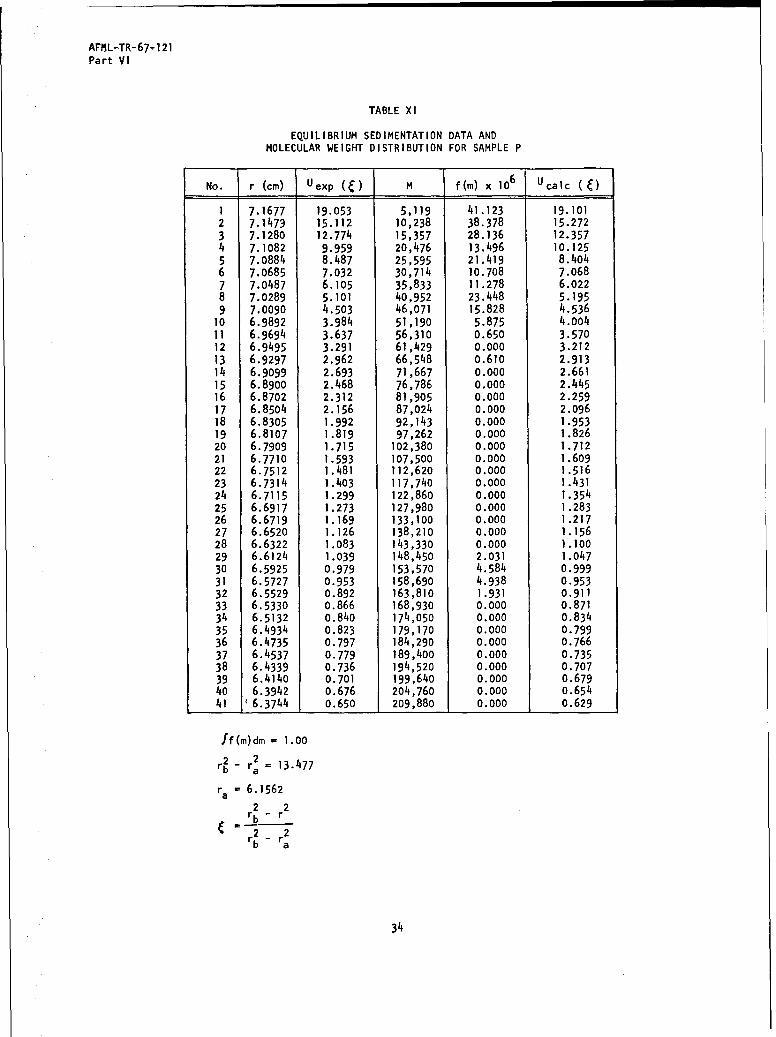
4. SAMPLE P
This was the Polydisperse sample, the prepared "known" distribution
of molecular weights. The purpose in choosing this particular
distribution will become apparent when we discuss the MWD obtained for
PBI in DMAC (see Section VI). This sample is a composite of Samples A,
B, and C. The relative concentration for each sample is A (56.9%),
B (34.1%), and C (9.0%). Because of these factors, the MWD for the
previous samples were not normalized to unity. To span the entire
molecular weight range O5m5180,000 and still keep a 41-point mesh (the
14
AFML-TR-67-121
Part VI
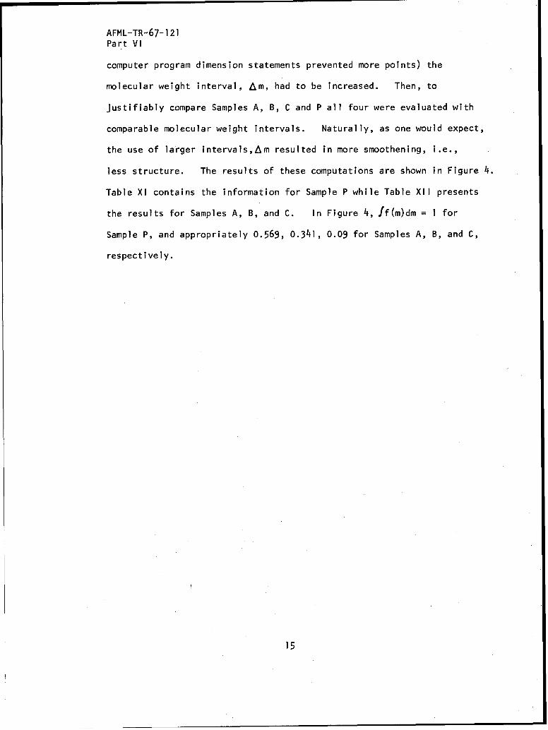
computer program dimension statements prevented more points) the
molecular weight interval, Am, had to be increased. Then, to
justifiably compare Samples A, B, C and P all four were evaluated with
comparable molecular weight intervals. Naturally, as one would expect,
the use of larger intervals,Am resulted in more smoothening, i.e.,
less structure. The results of these computations are shown in Figure 4.
Table XI contains the information for Sample P while Table XII presents
the results for Samples A, B, and C. In Figure 4, ff(m)dm = 1 for
Sample P, and appropriately 0.569, 0.341, 0.09 for Samples A, B, and C,
respectively.
15

AFML-TR-67-121
Part VI
SECTION VI
APPLICATION OF THE NEW METHOD FORMWD DETERMINATION OF PBI
Poly-(5,5'bibenzimidazole 2,2'diyl,l,3-phenylene) was synthesized
by Celenese Corp, Summit, New Jersey, in a melt reaction between
diamenobenzidine (DAB) and the diphenyl ester of isophtalic acid. This
sample is designated PBI-M. This PBI-M was purified as suggested by
T. E. Helminiak (Reference 13) and dried in a vacuum oven at 120%C and
0.01 Torr (C.L. Benner, Reference 14). This sample is designated
PBI-MPD (PBI-M purified and dried). Since the solute and the solvent
are very hygroscopic , the solutions were stored in sealed containers
under a blanket of nitrogen. If transferred they were continuously
flushed with nitrogen.
PBI-MPD in DMAC-solutions were investigated with the aid of a
Spinco Analytical Ultracentrifuge Model E. Experiments were performed
at 4T C and consisted of velocity (synthetic boundary) and equilibrium
sedimentation types. Necessary auxiliary measurements were also made
at 400C. The data used for the present PBI computation (regularization-
linear programing method) was the same as presented in Reference 7,
labeled "experimental." The result of this evaluation can be seen in
Figure 5 with the numerical tabulations given in Table XII1. Since
this curve (Figure 5) was obtained before the artificial MWD (Sample P,
Figure 4) was created, it should be immediately obvious that the
research with polystyrene was initiated to substantiate the regularization-
linear programing method which the authors have recently proposed
(References 2 and 4).
16

AFML-TR-67-121
Part VI
SECTION VII
CONCLUSIONS
The importance of this presentation is threefold.
1. Three polystyrene fractions, which were expected to be pure
and narrow, were investigated. Well known, well established experi-
mental methods were applied to determine the molecular weight average
of each fraction. By implementing such a procedure, the degree of
confidence in the experimental techniques was established. The two
experimental methods used were performed with the aid of an analytical
ultracentrifuge. One method is called the velocity (or synthetic
boundary) and the other sedimentation equilibrium. Even though the
same instrument was used for each method, the theoretical basis for
each is entirely different. After excellent comparison of the two
methods, a polydisperse molecular weight distribution was constructed
with these same fractions. The same experimental precautions used for
the individual fractions, were .now applied to the Polydisperse sample
during a sedimentation equilibrium experiment.
2. Within the past year or two AFML has developed a mathematical
procedure (References 1 through 4) for inferring the molecular weight
distribution of a polymer in solution, given data obtained from a
sedimentation equilibrium experiment at a single angular speed. Prior
to this time a feasible solution to the mathematically improperly posed
problem of inferring a molecular weight distribution from sedimentation
equilibrium data had not been achieved. When the method of regularization
was initially applied to this problem, all initial molecular weight
17
AFML-TR-67-121
Part VI
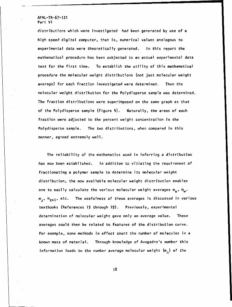
distributions which were investigated had been generated by use of a
high speed digital computer, that is, numerical values analogous to
experimental data were theoretically generated. In this report the
mathematical procedure has been subjected to an actual experimental data
test for the first time. To establish the utility of this mathematical
procedure the molecular weight distributions (not just molecular weight
average) for each fraction investigated were determined. Then the
molecular weight distribution for the Polydisperse sample was determined.
The fraction distributions were superimposed on the same graph as that
of the Polydisperse sample (Figure 4). Naturally, the areas of each
fraction were adjusted to the percent weight concentration in the
Polydisperse sample. The two distributions, when compared in this
manner, agreed extremely well.
The reliability of the mathematics used in inferring a distribution
has now been established. In addition to vitiating the requirement of
fractionating a polymer sample to determine its molecular weight
distribution, the now available molecular weight distribution enables
one to easily calculate the various molecular weight averages mn, mw-
mz, mz+1, etc. The usefulness of these averages is discussed in various
textbooks (References 15 through 19). Previously, experimental
determination of molecular weight gave only an average value. These
averages could then be related to features of the distribution curve.
For example, some methods in effect count the number of molecules in a
known mass of material. Through knowledge of Avogadro's number this
information leads to the number average molecular weight (m n) of the
18
AFML-TR-67-121
Part VI
sample. For the distribution of molecular weights of typical polymers
the number average lies near the peak of the curve or the most probable
molecular weight. In other experiments the weight average molecular
weight (m w) results. Here the heavy molecules are favored in the
averaging process. Finally the ratio mw/mn would be a measure of the
polydispersity of the molecular weight distribution.
Another benefit in knowing the molecular weight distribution is
evidenced in determining a viscosity average molecular weight. This
viscosity average is quite often wrongly replaced by the weight average
molecular weight, thus making the results from viscosity measurements
less precise.
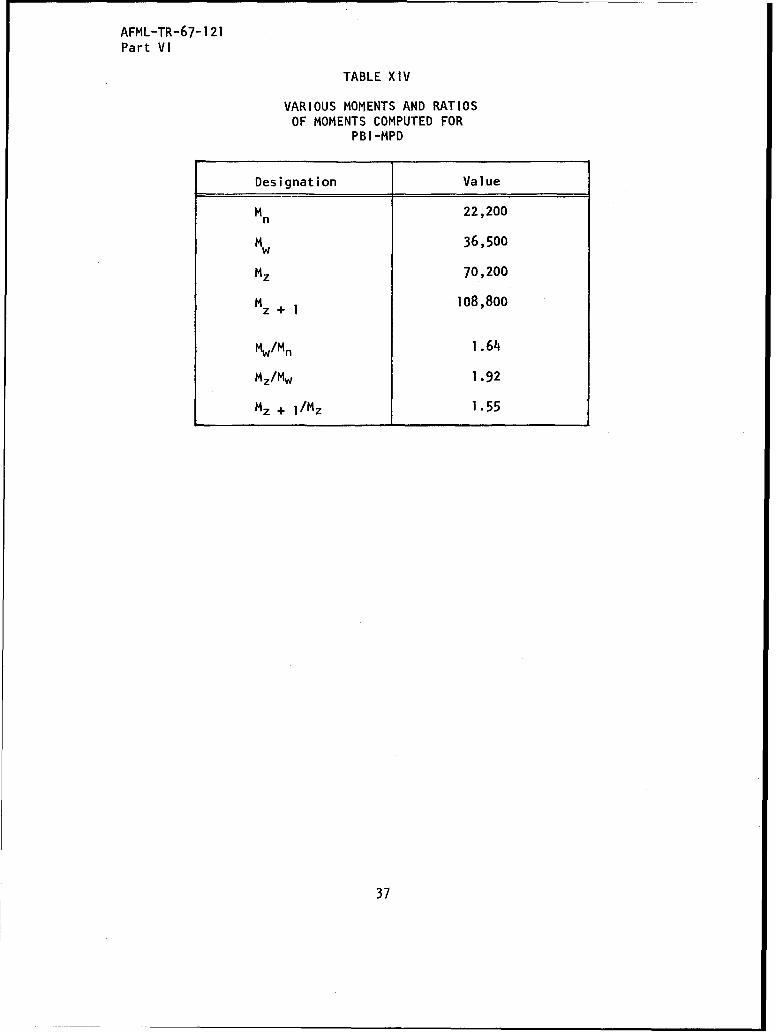
3. The molecular weight distribution for PBI-MPD (see Section VI
and Figure 5) has been determined. Various moments such as mn, mw,
mz, mz+l and their ratios have been computed. These results are
presented in Table XIV. The major concern now is the reliability of
a material such as PBI-MPD (Reference 2). Since the method (experi-
mental and mathematical) has been proved, the next step is to obtain
molecular weight distribution of PBI being used in applications in an
attempt to determine whether or not a relationship between MPD and the
reliability of the polymer material under use conditions can be
elucidated.
19

AFML-TR-67-121Part VI
REFERENCES
1. M. T. Gehatia and D. R. Wiff, AFML-TR-67-121, Part IV, Air ForceMaterials Laboratory, Wright-Patterson Air Force Base, Ohio(August 1970).
2. D. R. Wiff and M. T. Gehatia, AFML-TR-67-121, Part V (February1971).
3. M. Gehatia and D. R. Wiff, J. Polymer Sci., Part A-2, 8, 2039-2050(1970).
4. D. R. Wiff and M. Gehatia, J. Macromolecular Sci. - PhysicsB6(2), 287 (March 1972).
5. A. N. Tikhonov, Dakl. Akad. Nauk. SSSR, 151, No. 3, 501 (1963).
6. J. S. Hadamard, Lectures on Cauchy's Problem, Dover PublicationsInc., New York (1952).
7. M. Gehatia and D. R. Wiff, AFML-TR-67-121, Part II (April, 1969).
8. R. R. Jurick, D. R. Wiff, and M. T. Gehatia, AFML-TR-67-121,Part III (May 1970).
9. Svedberg and K. 0. Pedersen, Die Ultrazentrifuge, Dresden UndLeipzig (1939), p 20.
10. M. T. Gehatia, Kolloid-Zeitschrift 167 No. 1, 1-17 (1959).
1H. J. W. Williams, Ultracentrifugal Analysis, Academic Press,New York (1963).
12. H. Fujita, Mathematical Theory of Sedimentation Analysis,Academic Press, New York (1962).
13. T. E. Helminiak, AFML Technical Report in preparation.
14. C. L. Benner, AFML-TR-70-7 (February 1970).
15. P. J. Flory, Principles of Polymer Chemistry, Cornell UniversityPress, Ithaca, New York (1953).
16. T. M. Birshtein and 0. B. Ptitsyn, Conformations of Macromolecules,Interscience Publishers, New York (1966).
17. M. V. Volkenstein, Configurational Statistics of Polymeric Chains,Interscience Publishers, New York (1963).
20

AFML-TR-67-121Part VI
REFERENCES (Contd)
18. H. Morawetz, Macromolecules in Solution, Interscience Publis hers,
New York (1966).
19. F. W. Bellmeyer, Textbook of Polymer Chemistry Interscience
Publishers, New iork (1957).
21

AFML-TR-67-121Part Vt
80-
a?-5 x 1060 M- 5700
106
x
E40
20
0 I I I
0 20 40 60 80Molecular Weight x 10-3
Figure 1. Molecular Weight Distribution for Sample A Using
O:m<lO0,O00, and Am=2381; ff(m)dm=0.569
22

AFML-TR-67-121Part VI
20
16
16 az=6 x 10
Mw- 38 000
12
x8
E
4
030 50 70 90
Molecular Weight x I0-3
Figure 2. Molecular Weight Distribution for Sample B Using15,000<m<5100,000, and Am=2024; ff(m)dm=0.341
23
AFML-TR-67-121Part VI
8
6 z - 7 x 10¹⁴
Mw= 148)000
24-x
2-
0 13 - --. T--150 17 190
Molecular Weight x 10-
Figure 3. Molecular Weight Distribution for Sample C UsinglO0,O0Sm5:S8O,O00, and Am=l910; ff(m)dm=O.090
24

AFML-TR-67-121Part VI
•az2 x 10 -- B'-bU---
a. - 4 x 101- Ca 061.5 x 10
60
S40
E
20
I
00 40 80 120 160
Molecular Weight x l-O3
Figure 4. Molecular Weight Distribution for Sample P (Am=5120)With a Superposition of the Molecular Weight Distributionsfor Samples A, B, and C (+r.m=4286). In this caseffp (m)dm= f[fA (m) + fB (m) + fc(m)]dm= 1
25

AFML-TR-67-1 21Part yr
Lr'%
C EEL-
0
410
CD C)a--4
r-44-
CD,
LL)
CD~ <0
LaJ
41
L-C
Lr% C14 C
,01 x .- )-
26 - 4

AFML-TR-67-121
Part VI
TABLE IV
VELOCITY SEDIMENTATION DATA FOR SAMPLE A
r texp 100
No. max H (sec) H2 B x 103
1 6.7630 6.27 0 2.544 4.1554
2 6.7637 5.58 120 3.211 2.7661
3 6.7644 4.84 240 4.268 2.0717
4 6.7650 4.39 360 5.189 1.6550
5 6.7763 3.44 770 8.453 0.9785
6 6.7769 3.26 890 9.407 0.8734
7 6.7782 2.84 1130 12.391 0.7184
8 6.7809 2.68 1370 13.928 0.6096
9 6.7895 2.53 1610 15.630 0.5290
10 6.7868 2.37 1850 17.790 0.4669
11 6.7941 2.24 2090 19.920 0.4177
12 6.8027 2.10 2330 22.680 0.3776
13 6.8073 2.10 2570 22.680 0.3444
14 6.7974 1.95 2810 26.320 0.3164
15 6.8126 1.90 3050 27.780 0.2925
H = 1.05233 Y= 0.06611
w= 1.755 x 10⁷s = 1.33 x lO-13D = 8.5 x 10⁻⁵
Mw = (8.286 x 10¹⁰) (s)to = 240 sec
27

AFML-TR-67-121Part VI
TABLE V
EQUILIBRIUM SEDIMENTATION DATA FOR SAMPLE A
No. r (cm) Uexp (•) m f(m) x 106 Ucalc ()
1 7.1941 3.209 2,381 89.071 3.1652 7.1720 2.490 4,762 76.422 2.4283 7.1500 1.962 7,143 46.878 1.9394 7.128o 1.622 9,524 20.477 1.6105 7.1059 1.406 11,905 5.121 1.3866 7.0839 1.252 14,286 0.000 1.2297 7.0619 1.068 16,667 0.000 1.1178 7.0398 1.009 19,048 0.000 1.0349 7.0178 0.959 21,429 0.000 0.97010 6.9957 0.910 23,810 0.000 0.91911 6.9737 0.871 26,190 0.000 0.87612 6.9517 0.839 28,571 0.000 0.84013 6.9296 0.807 30,952 0.000 0.80814 6.9076 0.783 33,333 0.000 0.78015 6.8856 0.760 35,714 0.000 0.75316 6.8635 0.737 38,095 0.000 0.72917 6.8415 0.708 40,476 0.000 0.70618 6.8194 0.680 42,857 0.000 0.68419 6.7974 0.660 45,238 0.000 0.66320 6.7754 0.64O 47,619 0.000 0.64321 6.7533 0.617 50,000 0.000 0.62422 6.7313 0.599 52,381 0.000 0.60623 6.7093 0.581 54,762 0.000 0.58924 6.6872 0.563 57,143 0.000 0.57225 6.6652 0.542 59,524 0.000 0.55626 6.6432 0.531 61,905 0.000 0.54127 6.6211 0.517 64,286 0.000 0.52628 6.5991 0.506 66,667 0.000 0.51129 6.5770 0.490 69,048 0.000 0.49730 6.5550 0.476 71,429 0.000 0.48431 6.5330 0.460 73,810 0.000 0.47132 6.5109 0.449 76,190 0.000 0.45933 6.4889 0.436 78,571 0.000 o.44734 6.4669 0.422 80,952 1.1906 0.43535 6.4448 0.411 83,333 0.814 0.42336 6.4228 0.401 85,714 0.232 0.41437 6.4007 0.388 88,095 0.228 0.40338 6.3787 0.372 90,476 0.000 0.39339 6.3567 0.358 92,857 0.000 0.38340 6.3346 0.352 95,238 0.000 0.37441 6.3126 0.345 97,619 0.000 0.365
rb- ra - 14.1006
r = 6.13630
ff(m)dm = 0.569
2 r2rb-
r2 -r2
a
28

AFML-TR-67-121
Part VI
TABLE VI
VELOCITY SEDIMENTATION DATA FOR SAMPLE B
texp
No. rmax H (sec) H x 103
1 6.6507 6.7454 0 2.1978 1.6430
2 6.6546 6.6086 120 2.2897 1.3651
'3 6.6586 5.2617 360 3.6121 1.0180
4 6.6685 4.8618 600 3.7922 0.8098
5 6.6771 4.3987 840 5.1682 0.6709
6 6.6817 4.0620 1080 6.0606 0.5718
7 6.6969 3.7358 1320 7.1654 0.4974
8 6.6983 3.5779 1560 7.8119 0.4396
9 6.7049 3.3990 1800 8.6558 0.3934
10 6.7115 3.2622 2040 9.3967 0.3556
11 6.7207 3.1570 2280 10.0331 0.3241
12 6.7412 2.8623 2760 12.2055 0.2746
13 6.7571 2.6519 3240 14.2187 0.2376
14 6.7723 2.5466 3720 15.4202 0.2088
15 6.7987 2.3362 4680 18.3217 0.1669
H = 1.05233 Y
f = 0.06611
W2 = 1.755 x Io7
s = 2.729 x 10⁻¹³
D = 5.373 x 10⁻⁷
M, = (8.286 x 10¹⁰) (s)
t = 600 sec
29

AFML-TR-67-121Part VI
TABLE VII
EQUILIBRIUM SEDIMENTATION DATA FOR SAMPLE B
No. r (cm) Uexp (C) M f(m) x 106 Ucaic (•)
1 7.1412 4.426 17,024 0.000 4.2962 7.1191 3.899 19,048 0.344 3.8713 7.0971 3.440 21,071 1.520 3.4984 7.0751 3.049 23,095 3.668 3.1695 7.0530 2.814 25,119 6.658 2.8786 7.0310 2.592 27,143 10.159 2.6217 7.0089 2.390 29,167 13.716 2.3928 6.9869 2.199 31,190 16.831 2.1879 6.9649 2.017 33,214 19.029 2.004
10 6.9428 1.841 35,238 19.938 1.84011 6.9208 1.711 37,262 19.308 1.69212 6.8988 1.582 39,286 17.142 1.55813 6.8767 1.450 41,310 13.658 1.43714 6.8547 1.320 43,333 9.358 1.32715 6.8326 1.246 45,357 5.046 1.22716 6.8106 1.158 47,381 1.831 1.13617 6.7880 1.081 49,405 0.425 1.05318 6.7665 1.002 51,429 0.000 0.97719 6.7445 0.927 53,452 0.000 0.90820 6.7225 0.863 55,476 0.012 0.84421 6.7004 0.802 57,500 0.259 0.78522 6.6784 0.749 59,524 0.293 0.73123 6.6564 0.699 61,548 0.219 0.68124 6.6343 0.646 63,571 0.088 0.63525 6.6123 0.597 65,595 0.000 0.59326 6.5902 0.556 67,619 0.000 0.55427 6.5682 0.516 69,643 0.056 0.51728 6.5462 0.477 71,667 0.002 0.48429 6.5241 0.444 73,690 0.000 0.45230 6.5021 0.413 75,714 0.000 0.42331 6.48oi 0.382 77,738 0.000 0.39632 6.4580 0.358 79,762 0.066 0.37133 6.4360 0.332 81,786 0.000 0.34834 6.4139 0.305 83,810 0.000 0.32635 6.3919 0.286 85,833 0.255 0.30636 6.3699 0.266 87,857 0.753 0.28737 6.3478 0.248 89,881 1.340 0.27038 6.3258 0.233 91,905 1.788 0.25339 6.3038 0.217 93,929 1.897 0.23840 6.2817 0.196 95,952 1.603 0.22441 6.2597 0.182 97,976 1.125 0.210
r - r2 13.219
r = 6.1694
ff(m)dm = 0.341
r2 r2rb - r
b a
30

AFML-TR-67-121
Part VI
TABLE VIII
VELOCITY SEDIMENTATION DATA FOR SAMPLE C
texp 100
No. rmax H (sec) -H-T- x 103
1 6.6586 9.58 0 1.09 1.290
2 6.6685 8.89 120 1.27 1.107
3 6.6718 8.42 240 1.41 0.967
4 6.6804 8.00 360 1.56 0.858
5 6.6850 7.58 480 1.74 0.771
6 6.6983 7.31 600 1.87 0.698
7 6.7049 6.84 720 2.14 0.638
8 6.7115 6.79 840 2.17 0.587
9 6.7247 6.16 1080 2.64 0.504
10 6.7512 5.42 1560 3.40 0.391
11 6.7776 4.95 2040 4.08 0.317
12 6.8074 4.47 2520 5.00 0.265
13 6.8391 4.16 3000 5.78 0.226
14 6.8669 3.89 3480 6.62 0.197
15 6.8967 3.63 3960 7.58 0.173
H = 1.05233 Y
f = o.o6611
W2 = 1.755 x 10⁷
s = 4.97 x 10⁻¹³
D = 3.152 x 10⁻⁷
Mw = (8.286 x 101°0)
to = 750 sec
31

AFML-TR-67-121Part VIl
TABLE IX
EQUILIBRIUM SEDIMENTATION DATA FOR SAMPLE C
No. r (cm) Uexp (C) M f(m) x 106 Ucalc (•)
1 7.1632 0.7290 101,900 0.000 0.73762 7.1412 0.6808 103,810 0.000 0.68823 7.1191 0.6384 105,710 0.000 0.64224 7.0971 0.5955 107,620 0.000 0.59955 7.0751 0.5577 109,520 0.000 0.55976 7.0530 0.5227 111,430 0.000 0.52267 7.0310 0.4897 113,330 0.000 0.48828 7.0089 0.4582 115,240 0.000 0.45609 6.9896 0.4284 117,140 0.000 0.4261
10 6.9649 0.4006 119,050 0.000 0.398311 6.9428 0.3744 120,950 0.000 0.372312 6.9208 0.3514 122,860 0.100 0.348213 6.8988 0.3289 124,760 0.198 0.325614 6.8767 0.3090 126,670 0.162 0.304615 6.8547 0.2902 128,570 0.000 0.285016 6.8326 0.2708 130,480 0.000 0.266717 6.8106 0.2540 132,380 0.000 0.249718 6.7886 0.2388 134,290 0.000 0.233819 6.7665 0.2241 136,190 0.000 O.218920 6.7445 0.2095 138,100 0.000 0.205021 6.7225 0.1953 140,000 0.245 0.192122 6.70O4 0.1817 141,900 1.864 0.180023 6.6784 0.1707 143,810 5.162 0.168724 6.6564 0.1608 145,710 7.117 0.158225 6.6343 0.1503 147,620 8.774 0.148326 6.6123 0.1398 149,520 7.475 0.139127 6.5902 0.1304 151,430 4.592 0.130528 6.5682 0.1205 155,240 1.595 0.122529 6.5462 0.1100 157,140 0.765 0.114930 6.5241 0.1037 159,050 0.741 0.107931 6.5021 0.0969 160,950 0.772 0.101332 6.4806 0.0906 162,860 0.589 0.095133 6.4580 0.0854 164,760 0.258 0.089434 6.4360 0.0796 166,670 0.000 0.084035 6.4139 0.0733 168,570 0.000 0.079036 6.3919 0.0681 168,570 0.189 0.074237 6.3699 0.0628 170,485 0.000 0.069738 6.3478 0.0587 172,380 0.000 0.065639 6.3258 0.0550 174,295 0.000 0.061740 6.3038 0.0518 176,190 0.000 0.058041 6.2817 0.0508 178,105 0.000 0.0545
2 2
rb ra = 13.559
r a 6.1495
ff(m)dm = 0.090
r2 - r2
b a
32

AFML-TR-67-121Part VI
TABLE X
COMPARISON OF WEIGHT AVERAGE MOLECULAR WEIGHTS
Measured Technique M. of Samplesby Used A BC
Mellon
Institute Viscosity 5,200 29,100 114,200
AFML/LNP Velocity Sedimentation 6,300 42,100 130,700
AFML/LNP Equilibrium SedimentationSvedberg-Pederson Method 5,600 36,700 146,500
AFML/LNP Equilibrium SedimentationRegularization-Linear Progwith Am - 1500 5,700 38,000 148,100
AFML/LNP Equilibrium SedimentationRegularization-Linear Progwith A m • 5000 7,100 37,700 148,600
33
AFIL-TR-67-121Part VI
TABLE Xl
EQUILIBRIUM SEDIMENTATION DATA ANDMOLECULAR WEIGHT DISTRIBUTION FOR SAMPLE P
No. r (cm) Uexp () f(m) x 106 Ucalc (•)
1 7.1677 19.053 5,119 41.123 19.1012 7.1479 15.112 10,238 38.378 15.2723 7.1280 12.774 15,357 28.136 12.3574 7.1082 9.959 20,476 13.496 10.1255 7.0884 8.487 25,595 21.419 8.4046 7.0685 7.032 30,714 10.708 7.0687 7.0487 6.105 35,833 11.278 6.0228 7.0289 5.101 40,952 23.448 5.1959 7.0090 4.503 46,071 15.828 4.536
10 6.9892 3.984 51,190 5.875 4.00411 6.9694 3.637 56,310 0.650 3.57012 6.9495 3.291 61,429 0.000 3.21213 6.9297 2.962 66,548 0.610 2.91314 6.9099 2.693 71,667 0.000 2.66115 6.8900 2.468 76,786 0.000 2.44516 6.8702 2.312 81,905 0.000 2.25917 6.8504 2.156 87,024 0.000 2.09618 6.8305 1.992 92,143 0.000 1.95319 6.8107 1.819 97,262 0.000 1.82620 6.7909 1.715 102,380 0.000 1.71221 6.7710 1.593 107,500 0.000 1.60922 6.7512 1.481 112,620 0.000 1.51623 6.7314 1.403 117,740 0.000 1.43124 6.7115 1.299 122,860 0.000 1.35425 6.6917 1.273 127,980 0.000 1.28326 6.6719 1.169 133,100 0.000 1.21727 6.6520 1.126 138,210 0.000 1.15628 6.6322 1.083 143,330 0.000 1.10029 6.6124 1.039 148,450 2.031 1.04730 6.5925 0.979 153,570 4.584 0.99931 6.5727 0.953 158,690 4.938 0.95332 6.5529 0.892 163,810 1.931 0.91133 6.5330 0.866 168,930 0.000 0.87134 6.5132 0.840 174,050 0.000 0.83435 6.4934 0.823 179,170 0.000 0.79936 6.4735 0.797 184,290 0.000 0.76637 6.4537 0.779 189,400 0.000 0.73538 6.4339 0.736 194,520 0.000 0.70739 6.4140 0.701 199,640 0.000 0.67940 6.3942 0.676 204,760 0.000 0.65441 16.3744 0.650 209,880 0.000 0.629
ff(m)dm = 1.00
2rb- r2 = 13.477b a
ra = 6.1562
2 2
2rb - rb a
34

AFML-TR-67-121Part VI
TABLE XII
MOLECULAR WEIGHT DISTRIBUTION OF SAMPLES A, B, AND C
No. M fA (m) x 106 fB(m) x 106 fc(m) x 106
1 4,286 79.275 0.000 0.0002 8,571 46.942 0.000 0.0003 12,857 4.875 0.000 0.0004 17,143 0.000 0.000 0.0005 21,429 0.000 0.000 0.0006 25,714 0.000 0.000 0.0007 30,000 0.000 1.534 0.0008 34,286 0.000 27.726 0.0009 38,571 0.000 35.972 0.00010 42,857 0.000 14.193 0.00011 47,143 0.000 0.148 0.00012 51,429 0.000 0.000 0.00013 55,714 0.000 0.000 0.00014 60,000 0.000 0.000 0.00015 64,286 0.000 0.000 0.00016 68,571 0.000 0.000 0.00017 72,857 0.000 0.000 0.00018 77,143 0.000 0.000 0.00019 81,429 0.719 0.000 0.00020 85,714 0.934 0.000 0.00021 90,000 0.014 0.000 0.00022 94,286 0.000 0.000 0.00023 98,571 0.000 0.000 0.00024 102,860 0.000 0.000 0.00025 107,140 0.000 0.000 0.00026 111,430 0.000 0.000 0.00027 115,710 0.000 0.000 0.00028 120,000 0.000 0.000 0.00029 124,290 0.000 0.000 0.00030 128,570 0.000 0.000 0.00031 132,860 0.000 0.000 0.00032 137,140 0.000 0.000 1.26133 141,430 0.000 0.000 3.54734 145,710 0.000 0.000 5.01835 150,000 0.000 0.000 5.00536 154,290 0.000 0.000 3.72437 158,570 0.000 0.000 1.93138 162,860 0.000 0.000 0.51439 167,140 0.000 0.000 0.00040 171,430 0.000 0.000 0.00041 175,710 0.000 0.000 0.000
ffA(m)dm = 0.569
I fB(m)dm = 0.341
ff c(m)dm = 0.090
35

AFML-TR-67-121Part VI
TABLE XIII
EQUILIBRIUM SEDIMENTATION DATA ANDMOLECULAR WEIGHT DISTRIBUTION FOR PBI-MPD
No. r (cm) Uexp x 103 M f(m) x 107 Ucalc (•) x 103
1 7.1860 48.18 13,333 7.197 47.412 7.1632 41.67 16,667 4.855 43.253 7.1404 37.81 20,000 2.137 39.544 7.1176 34.84 23,333 0.000 36.255 7.0948 32.38 26,667 0.000 33.326 7.0720 30.02 30,000 0.000 30.707 7.0492 28.08 33,333 1.145 28.378 7.0264 26.16 36,667 2.314 26.289 7.0035 24.57 40,000 2.901 24.41
10 6.9807 22.96 43,333 2.547 22.7211 6.9579 21.48 46,667 1.343 21.2112 6.9351 20.22 50,000 0.000 19.8513 6.9123 19.14 53,333 0.000 18.6114 6.8895 18.12 56,667 0.000 17.5015 6.8667 17.14 60,000 0.000 16.4916 6.8439 16.33 63,333 0.000 15.5717 6.8211 15.41 66,667 0.000 14.7418 6.7983 14.63 70,000 0.000 13.9719 6.7754 13.92 73,333 0.000 13.2820 6.7526 13.36 76,667 0.000 12.6421 6.7298 12.68 80,000 0.000 12.0522 6.7070 12.00 83,333 0.000 11.5123 6.6842 11.54 86,667 0.000 11.0124 6.6614 11.01 90,000 0.000 10.5525 6.6386 10.58 93,333 0.000 10.1226 6.6158 10.08 96,667 0.000 9.7327 6.5930 9.68 100,000 0.000 9.3528 6.5702 9.21 103,333 0.000 9.0129 6.5473 8.89 106,667 0.000 8.6930 6.5245 8.53 110,000 0.000 8.3931 6.5017 8.32 113,333 0.000 8.1132 6.4789 7.92 116,667 0.000 7.8433 6.4561 7.67 120,000 0.000 7.5934 6.4333 7.41 123,333 0.000 7.3535 6.4105 7.20 126,667 0.000 7.1336 6.3877 6.95 130,000 0.000 6.9237 6.3649 6.73 133,333 0.000 6.7238 6.3421 6.51 136,667 1.191 6.5239 6.3192 6.29 140,000 1.365 6.3440 6.2964 6.07 143,333 0.000 6.1741 6.2736 5.89 146,667 0.000 6.00
ra = 6.0455
r- = 15.0908b a.
r2 r2b
r 2 r2b a
36
AFML-TR-67-121
Part VI
TABLE XIV
VARIOUS MOMENTS AND RATIOSOF MOMENTS COMPUTED FOR
PBI-MPD
Designation Value
M n22,200
MW 36,500
Mz 70,200
Mz + 1 108,800
Mw/Mn 1.64
Mz/Mw 1.92
Mz + i/Mz 1.55
37

UNCLASSIFIEDSecurity Classification
DOCUMENT CONTROL DATA - R & D(Security classification of title, body of abstract and indexing annotation must be entered when the overall report is classified)
I- ORIGINATING ACTIVITY (Corporate author) S2. REPORT SECURITY CLASSIFICATION
Air Force Materials Laboratory L••nc las ifiedWright-Patterson AFB, Ohio 45433 2b. OUP
3. REPORT TITLE
EVALUATION OF MOLECULAR WEIGHT FROM EQUILIBRIUM SEDIMENTATIONPART VI. EXPERIMENTAL VERIFICATION OF PREVIOUSLY PROPOSED REGULARIZATION-LINEAR
PROGRAMING, TFCHNIOIIIF WITH APP IRCATI(TN TI PRI4. DESCRIPTIVE NOTES (Type of report and inclusive dates)
Si'mmnrv R•_nnrt (flmrmhmr 1q7fl tn Ma~y 1971)lS. AU THORI•) (Firit name, mliddle initial, last name)-" "
Matatiahu T. GehatiaDonald R. Wiff
6. REPORT DATE 70 TOTAL NO4YF PAGESNovember 1971 . 19
On. CONTRACT OR GRANT NO. 9a. ORIGINATOR'S REPORT NUMBER(S)
b. PROJECT No. 7342 AFML-TR-67-121, Part VI
Task No. 734203 Sb. OTHER REPORT NO(SI (Any other number that may be assignedthis report)
d.
10. DISTRIBUTION STATEMENT
Approved for public release; distribution unlimited.
It. SUPPLEMENTARY NOTES 12. SPONSORING MILITARY ACTIVITYAir Force Materials LaboratoryWright-Patterson AFB, Ohio 45433
13. ABSTRACT
Experimental verification of the solution associated with the mathematicallyimproperly posed problem of inferring a molecular weight distribution fromequilibrium sedimentation data has been achieved. This was accomplished byinvestigating narrow linear polystyrene fractions and then superimposing thesefractions to create a known molecular weight distribution.
It has been shown that the previously proposed regularization-linear programingtechnique used to infer a molecular weight distribution produces a reliable solution.This technique was then applied to data obtained for PBI in DMAC. The results showthat an unusually large part of this polymer is of very low molecular weight. Howthis low molecular weight will affect the strength and reliability of PBI shouldwarrant further investigation.
DDFORMDD ,NOV 1473 UNCLASSIFIEDSecurity Classification

Secutyla~sisi~nction____________
1tINK A LINK * LINK CKEY WORDS
ROLE WT ROLE WT ROLE WT
Ul tracentri fugat ion
Equilibrium Sedimentation
Polydispersity
Improperly Posed Problems
Tikhonov's Regularization Method
Linear Programing
Molecular Weight Distribution
Polystyrene
PBI
Polymers
*U.S.Government Printing Office: 1972 - 759-081/296 UNCLAS-sIpirpSecurity Classification