Part II TGD - Europa
337
on Risk Assessment Part II Directive 98/8/EC of the European Parliament and of the Council concerning the placing of biocidal products on the market Commission Regulation (EC) No 1488/94 on Risk Assessment for existing substances Commission Directive 93/67/EEC on Risk Assessment for new notified substances in support of TGD Part II Institute for Health and Consumer Protection European Chemicals Bureau EUR 20418 EN/2 EUROPEAN COMMISSION JOINT RESEARCH CENTRE Technical Guidance Document
Transcript of Part II TGD - Europa

on Risk Assessment
Commission Regulation (EC) No 1488/94 on Risk Assessment for existing substances
Commission Directive 93/67/EEC on Risk Assessment for new notified substances
in support of
TGD
Part II
Institute for Health and Consumer Protection
European Chemicals Bureau
Technical Guidance Document
Directive 98/8/EC of the European Parliament and of the Council concerning the placing of biocidal products on the market
I
Part IEUR 20418 EN/2
EUROPEAN COMMISSION JOINT RESEARCH CENTRE

European Commission
Technical Guidance Document on Risk Assessment
in support of
Commission Directive 93/67/EEC on Risk Assessment
for new notified substances
Commission Regulation (EC) No 1488/94 on Risk Assessment
for existing substances
Directive 98/8/EC of the European Parliament and of the Council
concerning the placing of biocidal products on the market
Part II

LEGAL NOTICE
Neither the European Commission nor any person acting on behalf of the Commission is responsible for the use which might
be made of the following information
A great deal of additional information on the European Union is available on the Internet.
It can be accessed through the Europa Server (http://europa.eu.int).
© European Communities, 2003 Reproduction is authorised provided the source is acknowledged.
Printed in Italy

FOREWORD
I am pleased to present this Technical Guidance Document which is the result of in-depth co-operative work carried out by experts of the Member States, the Commission Services, Industry and public interest groups. This Technical Guidance Document (TGD) supports legislation on assessment of risks of chemical substances to human health and the environment. It is based on the Technical Guidance Document in support of the Commission Directive 93/67/EEC on risk assessment for new notified substances and the Commission Regulation (EC) No. 1488/94 on risk assessment for existing substances, published in 1996. This guidance was refined taking into account the experience gained when using it for risk assessments of about 100 existing substances and hundreds of new substances. Furthermore, it has been extended to address some of the needs of the Biocidal Products Directive (Directive 98/8/EC of the European Parliament and of the Council).
Concerning Chapter 2 on Risk assessment for human health, the Exposure assessment (Assessment of workplace exposure and Consumer exposure assessment) as well as the Effects assessment were improved and refined. However, for the following sections the revision process is not yet finalised and thus, the current TGD version uses the previous text: section 2.4 on Assessment of indirect exposure via the environment and section 4 on Risk characterisation. These sections are expected to be available by the end of 2003.
With respect to Chapter 3 on Environmental risk assessment, the Environmental exposure assessment and the Effects assessment underwent major improvements. A new chapter on Marine risk assessment was added.
Concerning Chapter 7, five out of eight available Emission scenario documents (ESDs) were revised (IC-3 Chemical industry: Chemicals used in synthesis, IC-7 Leather processing industry; IC-8 Metal extraction industry, refining and processing industry; IC-10 Photographic industry; IC-13 Textiles processing industry). Furthermore, a document on Rubber industry (IC-15) and a number of ESDs for the Biocidal Product Types or parts thereof were added. Some of the Emission scenario documents are still subject to on-going consultation in the OECD and thus, may need to be revised at a later stage. In addition, ESDs to cover all 23 Biocidal Product Types are under development. Consequently, it is anticipated that the set of Emission scenario documents will be continuously expanding in the future.
The White Paper outlining a future chemicals policy was adopted in February 2001 by the Commission. This TGD is therefore to be used in support of the current legislative instruments as described above until they are revoked and replaced by the future legislation implementing the White Paper.
I hope you will agree that this TGD makes a valuable contribution to the development and harmonisation of risk assessment methodologies not only within the Community but also worldwide in the context of the activities of the Organisation of Economic Co-operation and Development and the WHO/ILO International Programme on Chemical Safety.
Ispra, April 2003
Kees van Leeuwen Director Institute for Health and Consumer Protection
III

OVERVIEW
This Technical Guidance Document is presented in four separate, easily manageable parts.
PART I
Chapter 1 General Introduction
Chapter 2 Risk Assessment for Human Health
PART II
Chapter 3 Environmental Risk Assessment
PART III
Chapter 4 Use of (Quantitative) Structure Activity Relationships
((Q)SARs)
Chapter 5 Use Categories
Chapter 6 Risk Assessment Report Format
PART IV
Chapter 7 Emission Scenario Documents
V


Chapter 3
ENVIRONMENTAL RISK ASSESSMENT


3
CONTENTS
1 GENERAL INTRODUCTION ...................................................................................................................... 7
1.1 BACKGROUND ..................................................................................................................................... 7
1.2 GENERAL PRINCIPLES OF ASSESSING ENVIRONMENTAL RISKS ...................................... 10
2 ENVIRONMENTAL EXPOSURE ASSESSMENT .................................................................................... 13
2.1 INTRODUCTION .................................................................................................................................. 132.1.1 Measured / calculated environmental concentrations .................................................................... 142.1.2 Relationship between PEClocal and PECregional ......................................................................... 15
2.2 MEASURED DATA ............................................................................................................................... 172.2.1 Selection of adequate measured data ............................................................................................. 172.2.2 Allocation of the measured data to a local or a regional scale ....................................................... 21
2.3 MODEL CALCULATIONS .................................................................................................................. 212.3.1 Introduction ................................................................................................................................... 212.3.2 Data for exposure models .............................................................................................................. 242.3.3 Release estimation ......................................................................................................................... 25
2.3.3.1 Life-cycle of substances .................................................................................................. 262.3.3.2 Types of emissions and sources ....................................................................................... 292.3.3.3 Release estimation ........................................................................................................... 302.3.3.4 Intermittent releases ......................................................................................................... 352.3.3.5 Emissions during service life of long-life articles ........................................................... 362.3.3.6 Emissions from waste disposal ........................................................................................ 402.3.3.7 Delayed releases from waste disposal and dilution in time ............................................. 41
2.3.4 Characterisation of the environmental compartments ................................................................... 412.3.5 Partition coefficients ...................................................................................................................... 44
2.3.5.1 Adsorption to aerosol particles ........................................................................................ 452.3.5.2 Volatilisation ................................................................................................................... 452.3.5.3 Adsorption/desorption ..................................................................................................... 46
2.3.6 Abiotic and biotic degradation rates .............................................................................................. 482.3.6.1 Hydrolysis ........................................................................................................................ 492.3.6.2 Photolysis in water .......................................................................................................... 502.3.6.3 Photochemical reactions in the atmosphere ..................................................................... 512.3.6.4 Biodegradation in a sewage treatment plant .................................................................... 512.3.6.5 Biodegradation in surface water, sediment and soil ........................................................ 532.3.6.6 Overall rate constant for degradation in surface water .................................................... 57
2.3.7 Elimination processes prior to the release to the environment ...................................................... 572.3.7.1 Wastewater treatment ...................................................................................................... 572.3.7.2 Waste disposal, including waste treatment and recovery ................................................ 65
2.3.8 Calculation of PECs ....................................................................................................................... 692.3.8.1 Introduction ..................................................................................................................... 692.3.8.2 Calculation of PEClocal for the atmosphere.................................................................... 722.3.8.3 Calculation of PEClocal for the aquatic compartment .................................................... 752.3.8.4 Calculation of PEClocal for sediment ............................................................................. 782.3.8.5 Calculation of PEClocal for the soil compartment .......................................................... 782.3.8.6 Calculation of concentration in groundwater .................................................................. 862.3.8.7 Calculation of PECregional ............................................................................................. 86
2.4 SUMMARY OF PECS DERIVED ........................................................................................................ 90
2.5 DECISION ON THE ENVIRONMENTAL CONCENTRATION USED FOR RISKCHARACTERISATION ........................................................................................................................ 91
4
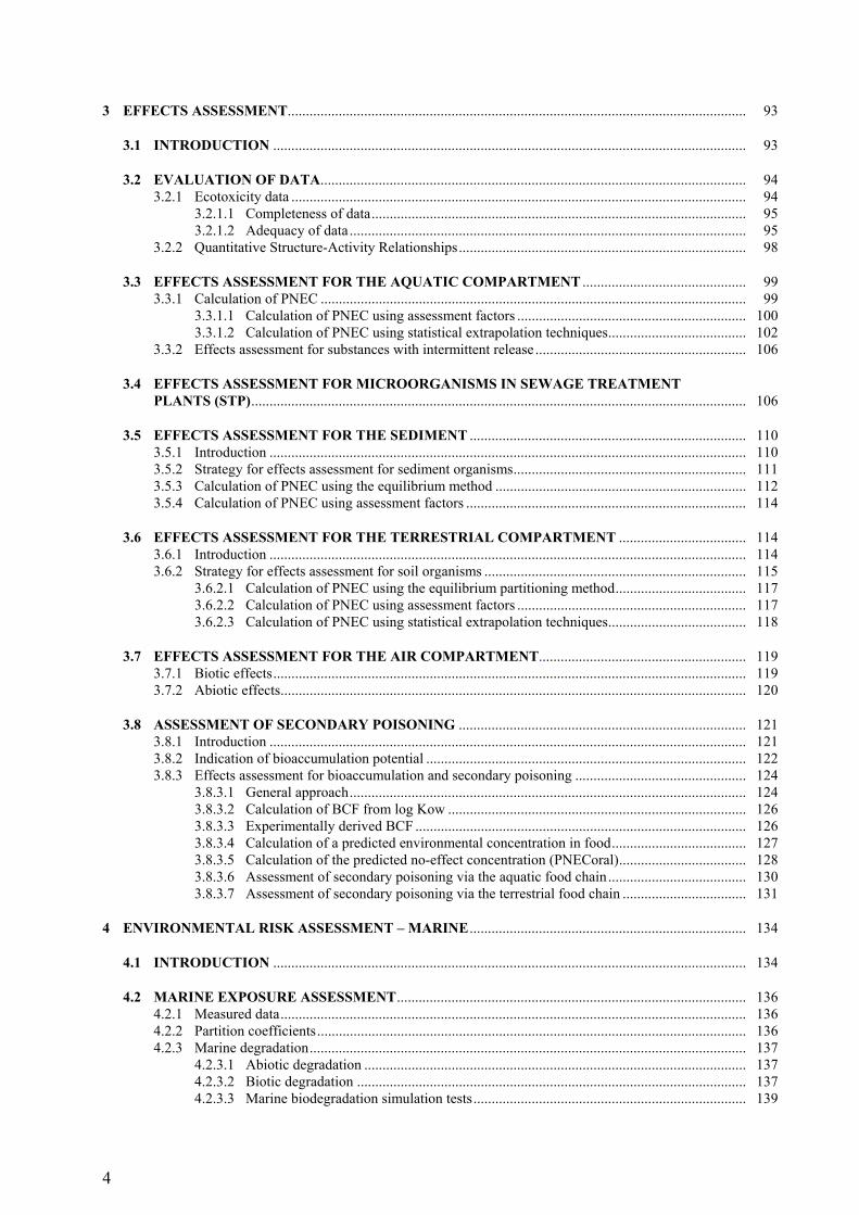
3 EFFECTS ASSESSMENT .............................................................................................................................. 93
3.1 INTRODUCTION .................................................................................................................................. 93
3.2 EVALUATION OF DATA..................................................................................................................... 943.2.1 Ecotoxicity data ............................................................................................................................. 94
3.2.1.1 Completeness of data ....................................................................................................... 953.2.1.2 Adequacy of data ............................................................................................................. 95
3.2.2 Quantitative Structure-Activity Relationships ............................................................................... 98
3.3 EFFECTS ASSESSMENT FOR THE AQUATIC COMPARTMENT ............................................. 993.3.1 Calculation of PNEC ..................................................................................................................... 99
3.3.1.1 Calculation of PNEC using assessment factors ............................................................... 1003.3.1.2 Calculation of PNEC using statistical extrapolation techniques ...................................... 102
3.3.2 Effects assessment for substances with intermittent release .......................................................... 106
3.4 EFFECTS ASSESSMENT FOR MICROORGANISMS IN SEWAGE TREATMENTPLANTS (STP) ........................................................................................................................................ 106
3.5 EFFECTS ASSESSMENT FOR THE SEDIMENT ............................................................................ 1103.5.1 Introduction ................................................................................................................................... 1103.5.2 Strategy for effects assessment for sediment organisms ................................................................ 1113.5.3 Calculation of PNEC using the equilibrium method ..................................................................... 1123.5.4 Calculation of PNEC using assessment factors ............................................................................. 114
3.6 EFFECTS ASSESSMENT FOR THE TERRESTRIAL COMPARTMENT ................................... 1143.6.1 Introduction ................................................................................................................................... 1143.6.2 Strategy for effects assessment for soil organisms ........................................................................ 115
3.6.2.1 Calculation of PNEC using the equilibrium partitioning method .................................... 1173.6.2.2 Calculation of PNEC using assessment factors ............................................................... 1173.6.2.3 Calculation of PNEC using statistical extrapolation techniques ...................................... 118
3.7 EFFECTS ASSESSMENT FOR THE AIR COMPARTMENT......................................................... 1193.7.1 Biotic effects .................................................................................................................................. 1193.7.2 Abiotic effects ................................................................................................................................ 120
3.8 ASSESSMENT OF SECONDARY POISONING ............................................................................... 1213.8.1 Introduction ................................................................................................................................... 1213.8.2 Indication of bioaccumulation potential ........................................................................................ 1223.8.3 Effects assessment for bioaccumulation and secondary poisoning ............................................... 124
3.8.3.1 General approach ............................................................................................................. 1243.8.3.2 Calculation of BCF from log Kow .................................................................................. 1263.8.3.3 Experimentally derived BCF ........................................................................................... 1263.8.3.4 Calculation of a predicted environmental concentration in food ..................................... 1273.8.3.5 Calculation of the predicted no-effect concentration (PNECoral) ................................... 1283.8.3.6 Assessment of secondary poisoning via the aquatic food chain ...................................... 1303.8.3.7 Assessment of secondary poisoning via the terrestrial food chain .................................. 131
4 ENVIRONMENTAL RISK ASSESSMENT – MARINE ............................................................................ 134
4.1 INTRODUCTION .................................................................................................................................. 134
4.2 MARINE EXPOSURE ASSESSMENT ................................................................................................ 1364.2.1 Measured data ................................................................................................................................ 1364.2.2 Partition coefficients ...................................................................................................................... 1364.2.3 Marine degradation ........................................................................................................................ 137
4.2.3.1 Abiotic degradation ......................................................................................................... 1374.2.3.2 Biotic degradation ........................................................................................................... 1374.2.3.3 Marine biodegradation simulation tests ........................................................................... 139

5
4.2.3.4 Use of biodegradation screening test data ....................................................................... 1394.2.4 Local Assessment .......................................................................................................................... 140
4.2.4.1 Introduction ..................................................................................................................... 1404.2.4.2 Calculation of PEClocal for the aquatic compartment .................................................... 1414.2.4.3 Calculation of PEClocal for the sediment compartment. ................................................. 144
4.2.5 Regional assessment ...................................................................................................................... 144
4.3 MARINE EFFECTS ASSESSMENT.................................................................................................... 1464.3.1 Effects Assessment for the aquatic compartment .......................................................................... 146
4.3.1.1 Introduction ..................................................................................................................... 1464.3.1.2 Evaluation of data ............................................................................................................ 1474.3.1.3 Derivation of PNEC ........................................................................................................ 148
4.3.2 Effects assessment for the sediment compartment ........................................................................ 1514.3.2.1 Introduction ..................................................................................................................... 1514.3.2.2 Strategy for effects assessment for sediment organisms .................................................. 1514.3.2.3 Calculations of PNEC for marine sediment using the equilibrium method ..................... 1534.3.2.4 Calculation of PNEC for marine sediment using assessment factors .............................. 154
4.3.3 Assessment of secondary poisoning .............................................................................................. 1574.3.3.1 Introduction ..................................................................................................................... 1574.3.3.2 Assessment of bioaccumulation and secondary poisoning .............................................. 1584.3.3.3 Testing strategy ............................................................................................................... 162
4.4 PBT ASSESSMENT ............................................................................................................................... 1624.4.1 Introduction ................................................................................................................................... 1624.4.2 PBT criteria .................................................................................................................................... 1634.4.3 Testing strategy for the P criterion ................................................................................................ 164
4.4.3.1 Introduction ..................................................................................................................... 1644.4.3.2 Experimental data on persistence in the marine environment ......................................... 1654.4.3.3 Other experimental data ................................................................................................... 1654.4.3.4 Data from biodegradation estimation models .................................................................. 1664.4.3.5 Summary of the P assessment .......................................................................................... 167
4.4.4 Testing strategy for the B criterion ................................................................................................ 1684.4.4.1 Introduction ..................................................................................................................... 1684.4.4.2 Assessment of measured BCF data .................................................................................. 1694.4.4.3 Assessment of the potential for bioaccumulation ............................................................ 1694.4.4.4 Other information relevant for assessment of the B criterion .......................................... 169
4.4.5 Testing strategy for the T criterion ................................................................................................ 1704.4.5.1 Introduction ..................................................................................................................... 1704.4.5.2 Chronic effects data ......................................................................................................... 1704.4.5.3 Acute effects data (screening level) ................................................................................. 1704.4.5.4 Estimated effects data ...................................................................................................... 171
5 RISK CHARACTERISATION...................................................................................................................... 172
5.1 INTRODUCTION .................................................................................................................................. 172
5.2 GENERAL PREMISES FOR RISK CHARACTERISATION .......................................................... 173
5.3 RISK CHARACTERISATION FOR EXISTING SUBSTANCES .................................................... 175
5.4 RISK CHARACTERISATION FOR NEW SUBSTANCES .............................................................. 176
5.5 RISK CHARACTERISATION FOR BIOCIDES ............................................................................... 179
5.6 QUALITATIVE RISK CHARACTERISATION ................................................................................ 179

6
6 TESTING STRATEGIES ............................................................................................................................... 181
6.1 INTRODUCTION .................................................................................................................................. 181
6.2 REFINEMENT OF PEC ........................................................................................................................ 1816.2.1 Aquatic compartment ..................................................................................................................... 1826.2.2 Soil compartment ........................................................................................................................... 1836.2.3 Air compartment ............................................................................................................................ 183
6.3 REFINEMENT OF PNEC: STRATEGY FOR FURTHER TESTING ............................................ 1846.3.1 Introduction ................................................................................................................................... 1846.3.2 Aquatic compartment ..................................................................................................................... 184
6.3.2.1 Introduction ..................................................................................................................... 1846.3.2.2 Available long-term tests ................................................................................................. 1866.3.2.3 Decision table for further testing ..................................................................................... 187
6.3.3 Sediment compartment .................................................................................................................. 1886.3.4 Soil compartment ........................................................................................................................... 190
7 REFERENCES ................................................................................................................................................ 194
Appendix I Emission factors for different use categories .............................................................................. 205Appendix II Fate of chemicals in a wastewater treatment plant based on the SimpleTreat model ................. 278Appendix III Evaluation of data ....................................................................................................................... 284Appendix IV Assignment of organisms to trophic levels ................................................................................. 287Appendix V Examples of assays suitable for further testing for soil organisms ............................................. 289Appendix VI Examples of assays suitable for futher testing for sediment organisms ...................................... 297Appendix VII Toxicity data for fish-eating birds and mammals ....................................................................... 300Appendix VIII Environmental risk assessment for metals and metal compounds .............................................. 301Appendix IX Environmental risk assessment for petroleum substances .......................................................... 311Appendix X Transformation pathways ........................................................................................................... 319Appendix XI Environmental risk assessment for ionising substances ............................................................. 320Appendix XII Connection to Sweage Treatment Plants in Europe .................................................................... 322Appendix XIII Risk assessment of sources not covered by the life-cycle of the substance ................................ 325Appendix XIV Information on the difference in diversity between saltwater and freshwater ............................ 327
GENERAL INTRODUCTION
7
1 GENERAL INTRODUCTION
1.1 BACKGROUND
Directive 93/67, Regulation 1488/94 and Directive 98/8 require that an environmental riskassessment be carried out on notified new substances, on priority existing substances and activesubstances and substances of concern in a biocidal product, respectively. This risk assessmentshould proceed in the following sequence:
• hazard identification;• dose (concentration) - response (effect) assessment;• exposure assessment;• risk characterisation.
The risk assessment shall be carried out for the three inland environmental compartments, i.e.aquatic environment, terrestrial environment and air, and for the marine environment.
The present document is intended to assist the competent authorities to carry out theenvironmental risk assessment of notified new substances, priority existing substances and activesubstances and substances of concern in a biocidal product. This guidance document includesadvice on the following issues:
• how to calculate Predicted Environmental Concentrations (PECs) (Sections 2 and 4.2) andPredicted No-Effect-Concentrations (PNECs) (Sections 3 and 4.3) and, where this is notpossible, how to make qualitative estimates of environmental concentrations and effect/noeffect concentrations;
• how to conduct a PBT (persistence, bioaccumulation and toxicity) assessment (Section 4.4);• how to judge which of the possible administrative decisions on the risk assessment
according to Article 3(4) of Directive 93/67, Article 10 of Regulation 793/93 and Annex Vof Regulation 1488/94 or Articles 10 and 11 of Directive 98/8 need to be taken (Section 5); and
• how to decide on the testing strategy, if further tests need to be carried out and how theresults of such tests can be used to revise the PEC and/or the PNEC (Section 6).
According to Article 9(2) of Regulation 793/93, the minimum data set that must be submitted forpriority existing substances is the base-set testing package required for notified new substanceswhich is defined in Annex VIIA of Directive 67/548. This ensures that for both notified new andpriority existing substances results from studies on short-term toxicity for fish, daphnia and algaeare available as a minimum. Hence, the procedure for calculating PNEC as well as the testingstrategy post base-set can use this as a starting point. For a new substance requirement ofadditional data is foreseen at level 1 and level 2 (Annex VIII of Directive 67/548). For existingsubstances information beyond the base-set may be available where the amount and quality ofdata may vary widely. For the effects assessment there may be several data available on a singleendpoint, which give dissimilar results. Furthermore, there may be studies, in particular olderstudies, which have not been conducted according to current test guidelines and qualitystandards. Expert judgement will be needed to evaluate the adequacy of these data.
Directive 98/8 (Article 8, Annex IIA and Annex IIIA) stipulates data requirements for biocidalactive substances. Annex IIA specifies core data requirements common to all active substances.Additional data requirements must be defined for each of 23 product types on the basis of AnnexIIIA. Specification of additional data requirements takes into account the characteristics of each

GENERAL INTRODUCTION
8
product type. The common core data requirements in Annex IIA together with the specific datarequirements in Annex IIIA constitute a complete set of data, adequate as a basis for riskassessment.
Due to the wide scope of the Biocidal Products Directive and the extensive variation of exposureand risks of different biocidal product types, the general rules given in the Directive and itsAnnexes have to be specified in order to ensure efficient and harmonised day-to-dayimplementation of the Directive. As written in Article 33, the Commission, in accordance withthe procedure laid down in Article 28(2), shall draw up technical notes for guidance to facilitatethe day-to-day implementation of this Directive.
Technical Notes for Guidance on data requirements for active substances and biocidal products(TNsG on Data Requirements, 2000; http://ecb.jrc.it/biocides/) give detailed practical guidanceon choice of studies and data reporting when applying for authorisation according to Directive98/8. It should be noted that only chemical biocidal products and substances are covered.Specific guidance is given on data requirements for substances of concern and in respect tosimplified procedures, i.e. those concerning frame-formulations, low-risk biocidal products andbasic substances.
Environmental exposure assessment is based on representative measured data and/or modelcalculations. If appropriate, available information on substances with analogous use andexposure patterns or analogous properties is taken into account. The availability ofrepresentative and reliable measured data and/or the amount and detail of the informationnecessary to derive realistic exposure levels by modelling, in particular at later stages in the life-cycle of a substance, will also vary. Again, expert judgement is needed.
In order to ensure that the predicted environmental concentrations are realistic, all availableexposure-related information on the substance should be used. When detailed information on theuse patterns, release into the environment and elimination, including information on thedownstream uses of the substance is provided, the exposure assessment will be more realistic. Ageneral rule for predicting the environmental concentration is that the best and most realisticinformation available should be given preference. However, it may often be useful to initiallyconduct an exposure assessment based on worst-case assumptions, and using default valueswhen model calculations are applied. Such an approach can also be used in the absence ofsufficiently detailed data. If the outcome of the risk characterisation based on worst-caseassumptions for the exposure is that the substance is not “of concern”, the risk assessment forthat substance can be stopped with regard to the compartment considered. If, in contrast, theoutcome is that a substance is “of concern”, the assessment must, if possible, be refined using amore realistic exposure prediction.
The guidance has been developed mainly from the experience gained on individual organicsubstances. This implies that the risk assessment procedures described cannot always be appliedwithout modifications to certain groups of substances, such as inorganic substances and metals.The methodologies that may be applied to assess the risks of metals and metal compounds,petroleum substances and ionisable substances are specifically addressed in appendices to thisguidance document (Appendix VIII, IX and XI, respectively). In these appendices, it is indicatedas much as possible where the text of the main document applies and where not. Wherenecessary, specific methods are described.
The risk assessments that have to be carried out according to Regulations 793/93 and 1488/94for existing substances, Directives 67/548 and 93/67 for new substances and Directive 98/8 foractive substances and substances of concern in a biocidal product, are in principle valid for all

GENERAL INTRODUCTION
9
countries in the European Union. It is recognised, however, that exposure estimation, forexample, is subject to variation due to topographical and climatological variability. Therefore, inthis document in the first stage of the exposure assessment where exposure models are used, so-called generic exposure scenarios are applied. These assume that substances are emitted into anon-existing model environment with predefined agreed environmental characteristics. Theseenvironmental characteristics can be average values or reasonable worst-case values dependingon the parameter in question. Generic exposure scenarios have been defined for local emissionsfrom a point source and for emissions into a larger region. In these generic scenarios emissionsto lakes are not assessed. When more specific information on the emission of a substance isavailable, it may well be possible to refine the generic or site-specific assessment.
Chapter 7 (Part IV) contains for a number of use categories so-called emission scenariodocuments (ESDs) that give more specific information on emissions to the environmentalcompartments that can occur during the use of a substance. Chapter 7 includes ESDs for sometypes of application of biocides while scenarios describing emissions of biocides from otherprocesses are still being developed. Such scenarios allow for quantitative emission estimation,which is an important first step in the exposure assessment, and generally has a significantinfluence on the outcome of risk assessments.
While comprehensive risk assessment schemes are presented for the aquatic and the terrestrialcompartment and for secondary poisoning, allowing a quantitative evaluation of the risk forthese compartments, the risk assessment for the air compartment can normally only be carriedout qualitatively because no standardised biotic testing systems are available at present. It shouldalso be noted that the schemes for the sediment and terrestrial compartments and for secondarypoisoning are currently not supported by the same level of experience and validation as availablefor the aquatic compartment. These schemes will need to be further reviewed and, if necessary,revised when new scientific knowledge and experience becomes available.
The test and assessment strategies in this Technical Guidance Document are based on the currentscientific knowledge and the experience of the competent authorities of the Member States. Inthis way, they reflect the best available scientific information to date and make use of the limiteddata set usually available. However, because this data set is limited, in particular for new andexisting substances where the data sets are restricted to acute toxicity testing with only threetrophic levels, there may be effects of substances that are not so well characterised in theassessment, such as:
• Adverse effects for which no adequate testing strategy is available yet (e.g. neurotoxicity,behavioural effects and endocrine disrupting effects);
• Specific effects in some taxa that cannot be modelled by extrapolation of the data of othertaxa (for example the specific effect of organotin compounds on molluscs).
For some substances the information on the environmental release from certain stages of the life-cycle, which may include the presence of the substance in preparations, is so scarce that the PECis quite uncertain or even not possible to estimate quantitatively. In the latter case a qualitativerisk assessment is conducted (see Section 5.6).
GENERAL INTRODUCTION
10
1.2 GENERAL PRINCIPLES OF ASSESSING ENVIRONMENTAL RISKS
The environmental risk assessment approach outlined in this chapter attempts to address theconcern for the potential impact of individual substances on the environment by examining bothexposures resulting from discharges and/or releases of chemicals and the effects of suchemissions on the structure and function of the ecosystem. Three approaches are used for thisexamination:
• quantitative PEC/PNEC estimation for environmental risk assessment of a substancecomparing compartmental concentrations (PEC) with the concentration below whichunacceptable effects on organisms will most likely not occur (predicted no effectconcentration (PNEC)). This includes also an assessment of food chain accumulation andsecondary poisoning;
• the qualitative procedure for the environmental risk assessment of a substance for thosecases where a quantitative assessment of the exposure and/or effects is not possible;
• the PBT assessment of a substance consisting of an identification of the potential of asubstance to persist in the environment, accumulate in biota and be toxic combined with anevaluation of sources and major emissions.
In principle, human beings as well as ecosystems in the aquatic, terrestrial and air compartmentare to be protected. At present, the environmental risk assessment methodology has beendeveloped for the following compartments:
For inland risk assessment:
• aquatic ecosystem (including sediment);• terrestrial ecosystem;• top predators;• microorganisms in sewage treatment systems;• atmosphere.
For marine risk assessment:
• aquatic ecosystem (including sediment);• top predators.
In addition to the three primary environmental compartments, effects relevant to the food chain(secondary poisoning) are considered. Also effects on the microbiological activity of sewagetreatment systems are considered. The latter is evaluated because proper functioning of sewagetreatment plants (STPs) is important for the protection of the aquatic environment.
The methodologies implemented have as aim the identification of acceptable or unacceptablerisks. This identification provides the basis for the regulatory decisions, which follow from therisk assessment. In some cases the uncertainties in carrying out the standard assessment becomeunacceptably high. The methodologies implemented in these cases are based on identifying theemission sources in order to identify where exposures should be minimised.
The PECs can be derived from available measured data and/or model calculations. The PNECvalues are usually determined on the basis of results from single species laboratory tests or, in afew cases, established effect and/or no-effect concentrations from model ecosystem tests, takinginto account adequate assessment factors. The PNEC can be derived using an assessment factorapproach or, when sufficient data is available, using the statistical extrapolation methods. A
GENERAL INTRODUCTION
11
PNEC is regarded as a concentration below which an unacceptable effect will most likely notoccur.
Dependent on the PEC/PNEC ratio the decision whether a substance presents a risk to organismsin the environment is taken. If it is not possible to conduct a quantitative risk assessment, eitherbecause the PEC or the PNEC or both cannot be derived, a qualitative evaluation is carried outof the risk that an adverse effect may occur.
As will be explained in more detail in the section on exposure assessment, PEC values arederived for local as well as regional situations, each of them based on a number of specificemission characteristics with respect to time and scale. As a consequence, the comparison ofPNEC values for the different compartments with different PEC values for different exposurescenarios can lead to a number of PEC/PNEC ratios.
In some cases, the current quantitative risk assessment approach does not provide sufficientconfidence that the environmental compartment or targets considered are sufficiently protected.The PBT assessment, given in Section 4.4, has been developed with the aim of identifying thesecases.
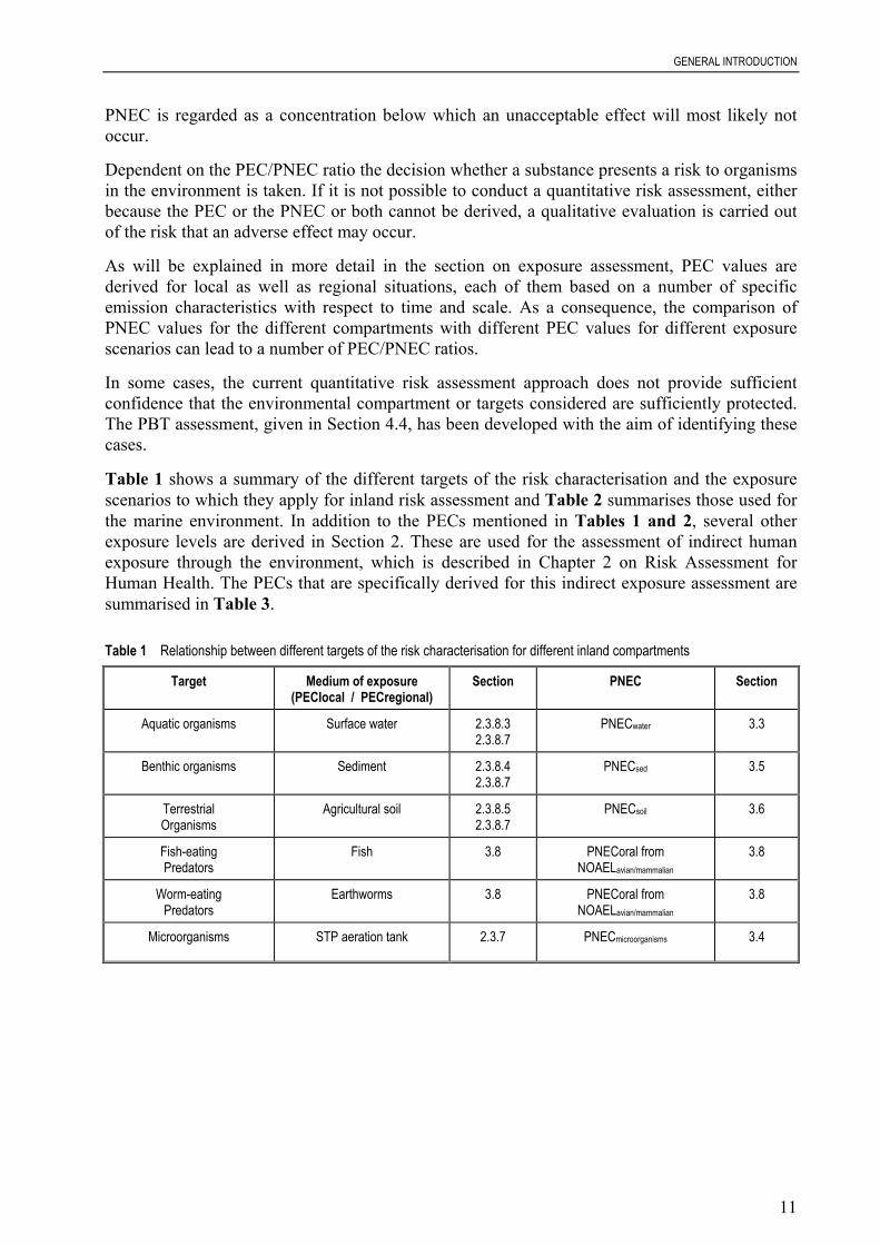
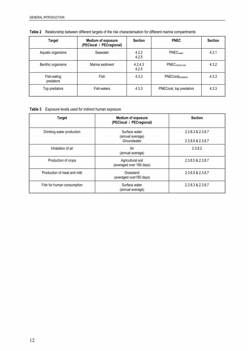
Table 1 shows a summary of the different targets of the risk characterisation and the exposurescenarios to which they apply for inland risk assessment and Table 2 summarises those used forthe marine environment. In addition to the PECs mentioned in Tables 1 and 2, several otherexposure levels are derived in Section 2. These are used for the assessment of indirect humanexposure through the environment, which is described in Chapter 2 on Risk Assessment forHuman Health. The PECs that are specifically derived for this indirect exposure assessment aresummarised in Table 3.
Table 1 Relationship between different targets of the risk characterisation for different inland compartments
Target Medium of exposure(PEClocal / PECregional)
Section PNEC Section
Aquatic organisms Surface water 2.3.8.32.3.8.7
PNECwater 3.3
Benthic organisms Sediment 2.3.8.42.3.8.7
PNECsed 3.5
TerrestrialOrganisms
Agricultural soil 2.3.8.52.3.8.7
PNECsoil 3.6
Fish-eatingPredators
Fish 3.8 PNECoral fromNOAELavian/mammalian
3.8
Worm-eatingPredators
Earthworms 3.8 PNECoral fromNOAELavian/mammalian
3.8
Microorganisms STP aeration tank 2.3.7 PNECmicroorganisms 3.4
GENERAL INTRODUCTION
12
Table 2 Relationship between different targets of the risk characterisation for different marine compartments
Target Medium of exposure(PEClocal / PECregional)
Section PNEC Section
Aquatic organisms Seawater 4.2.24.2.5
PNECwater 4.3.1
Benthic organisms Marine sediment 4.2.4.34.2.5
PNECmarine sed 4.3.2
Fish-eatingpredators
Fish 4.3.3 PNECoralpredators 4.3.3
Top predators Fish-eaters 4.3.3 PNECoral, top predators 4.3.3
Table 3 Exposure levels used for indirect human exposure
Target Medium of exposure(PEClocal / PECregional)
Section
Drinking water production Surface water(annual average)
Groundwater
2.3.8.3 & 2.3.8.7
2.3.8.6 & 2.3.8.7
Inhalation of air Air(annual average)
2.3.8.2
Production of crops Agricultural soil(averaged over 180 days)
2.3.8.5 & 2.3.8.7
Production of meat and milk Grassland(averaged over180 days)
2.3.8.5 & 2.3.8.7
Fish for human consumption Surface water(annual average)
2.3.8.3 & 2.3.8.7

ENVIRONMENTAL EXPOSURE ASSESSMENT
13
2 ENVIRONMENTAL EXPOSURE ASSESSMENT
2.1 INTRODUCTION
The environment may be exposed to chemical substances during all stages of their life-cyclefrom production to disposal or recovery. For each environmental compartment (air, soil, water,sediment) potentially exposed, the exposure concentrations should be derived. The assessmentprocedure should in principle consider the following stages of the life-cycle of a substance:
• production;• transport and storage;• formulation (blending and mixing of substances in preparations);• industrial/Professional use (large scale use including processing (industry) and/or small
scale use (trade));• private or consumer use;• service life of articles;• waste disposal (including waste treatment, landfill and recovery).
When assessing the exposure of the environment to existing chemicals, previous releases of thechemical to the environment need to be considered. These releases may have a cumulative effectthat gives rise to a “background concentration” in the environment.
Exposure may also occur from sources not directly related to the life-cycle of the substancebeing assessed. Examples of such sources are substances of natural origin, substances formed incombustion processes and other indirect emissions of the substance (e.g. as by-product,contaminant or degradation product of another substance). These kinds of sources have beenreferred to as “unintentional sources”. Guidance on how to deal with emissions not covered by thelife-cycle of the priority existing substance or biocidal active substance is given in Appendix XIII.
In view of uncertainty in the assessment of exposure of the environment, the exposure levelsshould be derived on the basis of both measured data, if available, and model calculations.Relevant measured data from substances with analogous use and exposure patterns or analogousproperties, if available, should also be considered when applying model calculations. Preferenceshould be given to adequately measured, representative exposure data where these are available(Sections 2.2.1 and 2.5).
Consideration should be given to whether the substance being assessed can be degraded,biotically or abiotically, to give stable and/or toxic degradation products. Where suchdegradation can occur, the assessment should give due consideration to the properties (includingtoxic effects) of the products that might arise. For new substances, it is unlikely that informationwill be available on such degradation products and thus only a qualitative assessment wouldnormally be possible. For existing substances and biocidal active substances, however, knownrelevant degradation products should also be subject to risk assessment. Where no information isavailable, a qualitative description of the degradation pathways can be made. A summary ofsome of these is presented in Appendix X. Furthermore it should be noted that guidance on howto assess and test relevant metabolites and transformation products is under preparation for plantprotection products under Directive 91/414. This guidance could be modified later for use forbiocides, and where appropriate for new and existing substances.
For many substances available biodegradation data is restricted to aerobic conditions. However,for some compartments, e.g. sediment or ground water, anaerobic conditions should also be

ENVIRONMENTAL EXPOSURE ASSESSMENT
14
considered. The same applies to anaerobic conditions in landfills and treatment of sewagesludge. Salinity and pH are examples of other environmental conditions that may influence thedegradation.
In the risk assessment a proper functioning of waste treatment is assumed. However, if thermaltreatment of waste is operated at insufficient technical conditions, organic substances may beformed having a PBT1 or POP profile. This may be the case in particular in the presence ofhalogens (Cl and Br) and catalysing metals (e.g. copper). If the formation of PBT or POPsubstances is identified as a special concern, this should be noted in the risk assessment. In thatcase it could be considered to add an appendix to the risk assessment report with furtherinformation on the possible formation of substances with a PBT or POP profile.
2.1.1 Measured / calculated environmental concentrations
No measured environmental concentrations will normally be available for new substances.Therefore, concentrations of a substance in the environment must be estimated. In contrast, theexposure assessment of existing substances does not always depend upon modelling. Data onmeasured levels in various environmental compartments have been gathered for a number ofexisting substances. They can provide the potential for greater insight into specific steps of theexposure assessment procedure (e.g. concentration in industrial emissions, “background”concentrations in specific compartments, characterisation of distribution behaviour). The specificguidance for existing and new chemicals given below should also be applied in general forbiocides.
In many cases, a range of concentrations from measured data or modelling will be obtained. Thisrange can reflect different conditions during manufacturing and use of the substance, or may bedue to assumptions in or limitations of the modelling or measurement procedures. It may seemthat measurements always give more reliable results than model estimations. However, measuredconcentrations can have a considerable uncertainty associated with them, due to temporal andspatial variations. Both approaches complement each other in the complex interpretation andintegration of the data. Therefore, the availability of adequate measured data does not imply thatPEC calculations are unnecessary.
For existing substances, the rapporteur should initially make the generic “reasonable worst-case”exposure assessment based on modelling, to derive an EU environmental concentration.Measured data, i.e., site-specific or monitoring information, can then be used to revise thecalculated concentrations. Other site-specific information such as effluent volumes, size of STP,river flow etc. may also be useful. In carrying out this revision, the rapporteur is recommendedto include in the exposure assessment of existing substances, a table containing availability ofsite-specific information for each production site (if limited in number) or group of productionsites (if numerous), as far as confidentiality issues allow. The “site-specific” concentrationsestimated may involve the use of actual site-specific information and more generic values (andpossibly extrapolated values as described below). The rapporteur should then consider in whichcases extrapolation is possible from sites with site-specific information to a site withoutinformation. Aspects to consider here include the proportion of the industry covered by specificinformation, the nature of the industry and information about its distribution, the comparativesize of sites, the types of process used etc. The rapporteur should justify in the risk assessment
1 Substances being persistent, bioaccumulative and toxic (PBT) or substances classified as a persistent organic
pollutant under the UN Stockholm Convention on Persistent Organic Pollutants.
ENVIRONMENTAL EXPOSURE ASSESSMENT
15
report the grounds on which the extrapolation has been done. It may be possible to extrapolatesome aspects but not others, for example emission factors (on the basis of similar processes) butnot effluent flows (on the basis of differing sizes of site). If no such extrapolation can bejustified, then the modelling approach described in the TGD should be followed for the (groupof) site(s).
For new substances, a generic assessment would normally be conducted. However, there may becircumstances where environmental exposure for some life-cycle stages is limited to specificsites (e.g. production of chemicals, processing of intermediates etc). It may, therefore, beadequate to carry out a site-specific risk assessment only, if the Competent Authority (CA) issatisfied that such specific information will enable a full evaluation of the risks. In such cases, itis the responsibility of the notifier to provide site-specific data and to show that the availableinformation is valid for the sites being assessed. The risk assessment should make clear that asite-specific assessment has been conducted. In these cases, the notifier is obliged to confirm inwriting that they will inform the CA of any relevant changes, which may affect the riskassessment conducted. The CA should confirm details of the assessment not later than two yearsafter completion of the risk assessment, and at any subsequent tonnage trigger, or as deemednecessary. The CA should distribute relevant information appropriately.
It should be noted that the site-specific risk assessment is not based on a detailed andcomplete description of the environmental conditions. The aim is to estimate environmentalconcentrations that are reasonably applicable for a European-level risk assessment. Somesite-specific data may be used to replace the default data characterising the standard scenario.
For measured data, the reliability of the available data has to be assessed as a first step.Subsequently, it must be established how representative the data are of the general emissionsituation. Section 2.2 provides guidance on how to perform this critical evaluation of measureddata. For model calculations, the procedure to derive an exposure level should be madetransparent. The parameters and default values used for the calculations must be documented. Ifdifferent models are available to describe an exposure situation, the best model for the specificsubstance and scenario should be used and the choice should be explained. If a model is chosenwhich is not described in this document, that model should be explained and the choice justified.Section 2.3 discusses modelling in detail. Section 2.5 gives further advice on critical comparisonbetween calculated and measured PECs.
2.1.2 Relationship between PEClocal and PECregional
For the release estimation of substances, a distinction is usually made between substances thatare emitted through point sources at specific locations and substances that enter the environmentthrough diffuse releases. Point source releases have a major impact on the environmentalconcentration on a local scale (PEClocal) and also contribute to the environmentalconcentrations on a larger scale (PECregional).
When determining a PEC for new substances at base-set level, or at the 10 tonnes per annumproduction level, Annex III, paragraph 3.4 of Directive 93/67 foresees that such estimates willusually focus on the generic local environment to which releases may occur. In the case ofpersistent and/or highly toxic chemicals, however, a regional assessment may still be relevant atlow tonnages. Therefore, derivation of a PECregional is required, unless it can be justified that aregional assessment is not relevant for the substance at these low tonnages.
ENVIRONMENTAL EXPOSURE ASSESSMENT
16
PEClocal
The concentrations of substances released from point sources are assessed for a generic localenvironment. This is not an actual site, but a hypothetical site with predefined, agreedenvironmental characteristics, the so-called “standard environment”. These environmentalconditions can be average values, or reasonable worst-case values, depending on the parameterin question. The scale is usually small and it is assumed that the targets are exposed in, or at theborder of, the area. In general, concentrations during an emission episode are measured orcalculated. This means that PEClocal is calculated on the basis of a daily release rate, regardlessof whether the discharge is intermittent or continuous. It represents the concentration expected ata certain distance from the source on a day when discharge occurs. Only for the soilcompartment (being a less dynamic environment than air or surface water) longer-term averagesapply. However, in some cases time related concentrations may be obtained, for instance insituations where intermittent releases occur. In principle, degradation and distribution processesare taken into consideration for the PEClocal. However, because of the relatively small spatialscale, only one or two key processes typically govern the ultimate concentration in acompartment.
PECregional
The concentrations of substances released from point and diffuse sources over a wider area areassessed for a generic regional environment. The PECregional takes into account the furtherdistribution and fate of the chemical upon release. It also provides a background concentration tobe incorporated in the calculation of the PEClocal. As with the local models, a generic standardenvironment is defined. The PECregional is assumed to be a steady-state concentration of thesubstance.
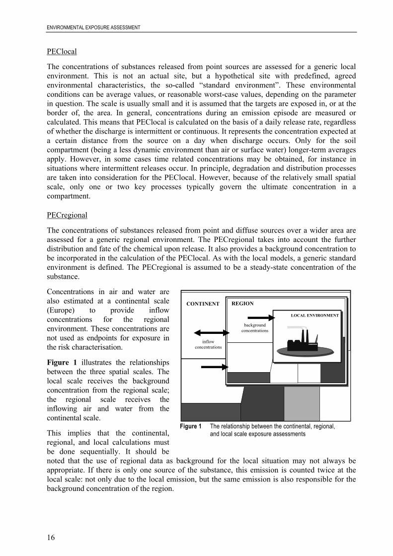
Concentrations in air and water arealso estimated at a continental scale(Europe) to provide inflowconcentrations for the regionalenvironment. These concentrations arenot used as endpoints for exposure inthe risk characterisation.
Figure 1 illustrates the relationshipsbetween the three spatial scales. Thelocal scale receives the backgroundconcentration from the regional scale;the regional scale receives theinflowing air and water from thecontinental scale.
This implies that the continental,regional, and local calculations mustbe done sequentially. It should benoted that the use of regional data as background for the local situation may not always beappropriate. If there is only one source of the substance, this emission is counted twice at thelocal scale: not only due to the local emission, but the same emission is also responsible for thebackground concentration of the region.
CONTINENT
LOCAL ENVIRONMENT
REGION
backgroundconcentrations
inflowconcentrations
Figure 1 The relationship between the continental, regional, and local scale exposure assessments

ENVIRONMENTAL EXPOSURE ASSESSMENT
17
2.2 MEASURED DATA
For a number of existing substances measured data are available for air, fresh or saline water,sediment, biota and/or soil. These data have to be carefully evaluated for their adequacy andrepresentativeness according to the criteria below. They are used together with calculatedenvironmental concentrations in the interpretation of exposure data.
The evaluation should follow a stepwise procedure:
• reliable and representative data should be selected by evaluation of the sampling andanalytical methods employed and the geographic and time scales of the measurementcampaigns (Section 2.2.1);
• the data should be assigned to local or regional scenarios by taking into account the sourcesof exposure and the environmental fate of the substance (Section 2.2.2);
• the measured data should be compared to the corresponding calculated PEC. For naturallyoccurring substances background concentrations have to be taken into account. For riskcharacterisation, a representative PEC should be decided upon based on measured data and acalculated PEC (Section 2.5).
2.2.1 Selection of adequate measured data
The available measured environmental concentrations have to be assessed first. The followingaspects could be considered in order to decide if the data are adequate for use in the exposureassessment and how much importance should be attached to them:
Quality of the applied measuring techniques
The applied techniques of sampling, sample shipping and storage, sample preparation foranalysis and analysis must consider the physico-chemical properties of the substance. Measuredconcentrations that are not representative as indicated by an adequate sampling programme orare of insufficient quality should not be used in the exposure assessment.
The limit of quantitation (LOQ) of the analytical method, which is normally defined by theanalytical technique being used, should be suitable for the risk assessment and the comparabilityof the measured data should be carefully evaluated. For example, the concentrations in watermay either reflect total concentrations or dissolved concentrations according to the sampling andpreparation procedures used. The concentrations in sediment may significantly depend on thecontent of organic carbon and particle size of the sampled sediment. The soil and sedimentconcentrations should preferably be based on concentrations normalised for the particle size (i.e.coarsest particles taken out by sieving). All measurements below the LOQ constitute a specialproblem and should be considered on a case-by-case basis. One approach that could beconsidered would be to use a value corresponding to LOQ/2 before estimating a mean orstandard deviation (EC, 1999). As this method could heavily influence the mean and standarddeviation, other methods may also be considered (e.g. assuming same distribution of data belowand above the LOQ).
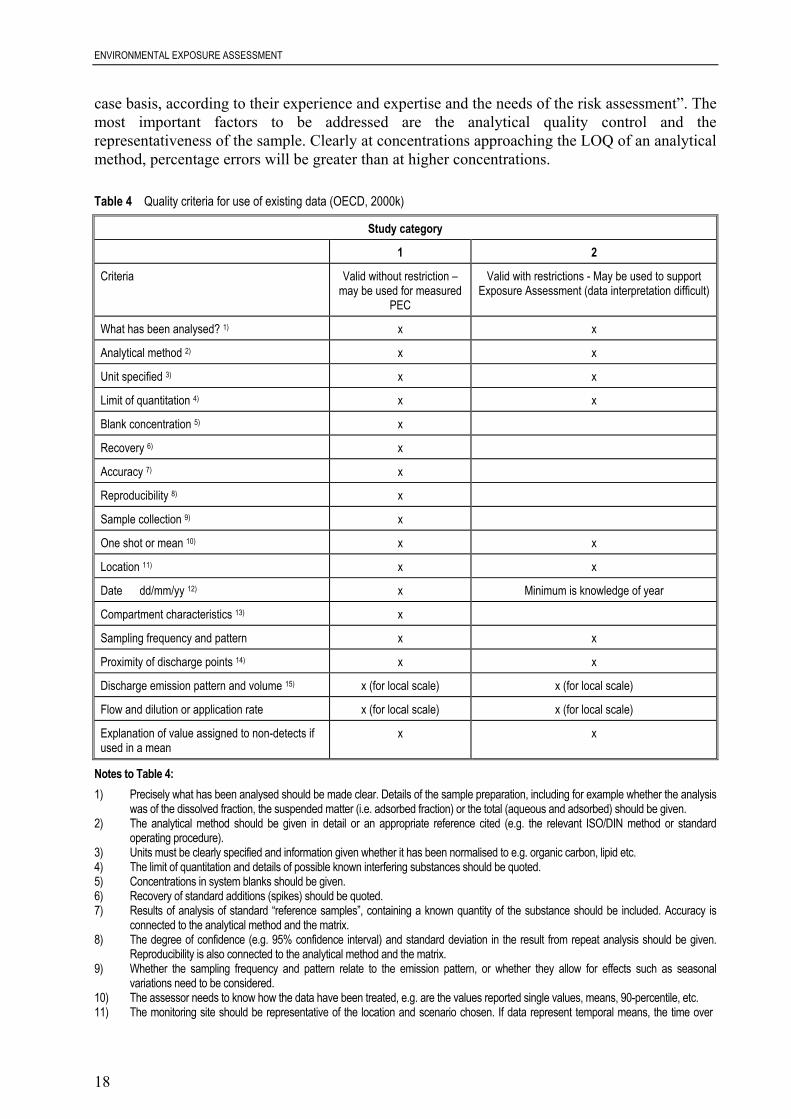
The aim is to obtain as much useful information on exposure from a data set as possible, butthere is inherent danger for inappropriate use of the data for risk assessment purposes. Toaddress this problem, two quality levels for existing data are given in Table 4 (taken fromOECD, 2000k). In recommending this table the OECD stressed “…these criteria should beapplied in a flexible manner. For example, data should not always be discounted because they donot meet the criteria. Risk assessors should make a decision to use the data or not, on a case-by-
ENVIRONMENTAL EXPOSURE ASSESSMENT
18
case basis, according to their experience and expertise and the needs of the risk assessment”. Themost important factors to be addressed are the analytical quality control and therepresentativeness of the sample. Clearly at concentrations approaching the LOQ of an analyticalmethod, percentage errors will be greater than at higher concentrations.
Table 4 Quality criteria for use of existing data (OECD, 2000k)
Study category
1 2
Criteria Valid without restriction –may be used for measured
PEC
Valid with restrictions - May be used to supportExposure Assessment (data interpretation difficult)
What has been analysed? 1) x x
Analytical method 2) x x
Unit specified 3) x x
Limit of quantitation 4) x x
Blank concentration 5) x
Recovery 6) x
Accuracy 7) x
Reproducibility 8) x
Sample collection 9) x
One shot or mean 10) x x
Location 11) x x
Date dd/mm/yy 12) x Minimum is knowledge of year
Compartment characteristics 13) x
Sampling frequency and pattern x x
Proximity of discharge points 14) x x
Discharge emission pattern and volume 15) x (for local scale) x (for local scale)
Flow and dilution or application rate x (for local scale) x (for local scale)
Explanation of value assigned to non-detects ifused in a mean
x x
Notes to Table 4:1) Precisely what has been analysed should be made clear. Details of the sample preparation, including for example whether the analysis
was of the dissolved fraction, the suspended matter (i.e. adsorbed fraction) or the total (aqueous and adsorbed) should be given.2) The analytical method should be given in detail or an appropriate reference cited (e.g. the relevant ISO/DIN method or standard
operating procedure).3) Units must be clearly specified and information given whether it has been normalised to e.g. organic carbon, lipid etc.4) The limit of quantitation and details of possible known interfering substances should be quoted.5) Concentrations in system blanks should be given.6) Recovery of standard additions (spikes) should be quoted.7) Results of analysis of standard “reference samples”, containing a known quantity of the substance should be included. Accuracy is
connected to the analytical method and the matrix.8) The degree of confidence (e.g. 95% confidence interval) and standard deviation in the result from repeat analysis should be given.
Reproducibility is also connected to the analytical method and the matrix.9) Whether the sampling frequency and pattern relate to the emission pattern, or whether they allow for effects such as seasonal
variations need to be considered.10) The assessor needs to know how the data have been treated, e.g. are the values reported single values, means, 90-percentile, etc.11) The monitoring site should be representative of the location and scenario chosen. If data represent temporal means, the time over
ENVIRONMENTAL EXPOSURE ASSESSMENT
19
which concentrations were averaged should be given too.12) The time, day, month and year may all be important depending upon the release pattern of the chemicals. Time of sampling may be
essential for certain discharge/emission patterns and locations. For some modelling and trends analysis, the year of sampling will bethe minimum requirements.
13) Compartment characteristics such as lipid content, content of organic carbon and particle size should be specified. 14) For the local aqueous environment, detailed information on the distance of other sources in addition to quantitative information on flow
and dilution are needed.15) It is necessary to consider whether there is a constant and continuous discharge, or whether the chemical under study is released as a
discontinuous emission showing variations in both volume and concentration with time.
When a substance is used in materials (e.g. polymers) it may be released to the environmentenclosed within the matrix of small particles of the material formed e.g. by weathering orabrasion (see 2.3.3.5). In such cases it would be useful to know if the analytical method used isable to detect also the fraction of substance that is associated with these particles. Theavailability for analysis can be expected to be reduced for resistant materials and/or largeparticles. Depending on use pattern, particles may end up in STP sludge/agricultural soil,sediments affected by storm water outflows, industrial/urban soil and indoor dust.
Selection of representative data for the environmental compartment of concern
There are two distinct aspects to consider:
The level of confidence in the result, i.e. the number of samples, how far apart and howfrequently they were taken. The sampling frequency and pattern should be sufficient toadequately represent the concentration at the selected site.
Whether the sampling site(s) represent a local or regional scenario. Samples taken at sitesdirectly influenced by an emission should be used to describe the local scenario, while samplestaken at larger distances may represent the regional concentrations.
It has to be ascertained if the data are results of sporadic examinations or if the substance wasdetected at the same site over a certain period of time. Measured concentrations caused by anaccidental spillage or malfunction should not be considered in the exposure assessment.
Where outliers have been identified their inclusion/exclusion should be discussed and justified.The data should be critically examined to establish whether high values reflect an increased ornew release, a recent change in emission pattern or a newly discovered occurrence in a specificenvironmental compartment. The data should also be examined to check that the analyticalmethodology was appropriate.
If many data are available, the following statistical approach for defining outliers may be used:
))log()(log()log()log( 257575 ppKpX i −+> (1)
Where Xi is the concentration, above which a measured value may be considered an outlier, pi isthe value of the ith percentile of the statistic and K is a scaling factor. This filtering of data with ascaling K = 1.5 is used in most statistical packages, but this factor can be subject dependent.
Data from a prolonged monitoring programme, where seasonal fluctuations are already included,are of special interest. If available, the distribution of the measured data could be considered foreach monitored site, to allow all the information in the distribution function to be used. Forregional PEC assessment, a further distribution function covering several sites could beconstructed from single site statistics (for example, median, or 90th percentile if the distribution

ENVIRONMENTAL EXPOSURE ASSESSMENT
20
function has only one mode), and the required 90th percentile values, mean or median values ofthis distribution could be used in the PEC prediction. The mean of the 90th percentiles of theindividual sites within one region is recommended for regional PEC determination. Care shouldbe taken that data from several sites obtained with different sampling frequencies should not becombined, without appropriate consideration of the number of data available from each site. Ifindividual measurements are not available then results expressed as means and giving standarddeviation will be of particular relevance because in most instances a log normal distribution ofconcentrations can be assumed and a 90th percentile concentration may be calculated. If onlymaximum concentrations are reported, they should be considered as a worst-case assumption,providing they do not correspond to an accident or spillage. However, use of only the meanconcentrations can result in an underestimation of the existing risk, because temporal and/orspatial average concentrations do not reflect periods and/or locations of high exposure.
For intermittent release scenarios, even the 90-percentile values may not properly addressemission episodes of short duration but of high concentration discharge. In these cases, mainlyfor PEClocal calculations, a more realistic picture of the emission pattern can be obtained fromthe highest value of average concentrations during emission episodes.
Representative measured data from monitoring programmes or from literature, for comparisonwith calculated PECs should be compiled as tables and annexed to the risk assessment report.The measured data should be presented in the following manner:
Location Substance Concentration Period Remark Reference
Country
− location
substance ormetabolite
Units: [µg/L], [ng/L][mg/kg], etc
Data- mean- average- range- percentile- daily- weekly- monthly- annual- etc
month, year limit of quantitation(LOQ)
relevant information onanalytical method
analytical quality control
Literature reference
When emissions of a substance from waste treatment or disposal stages are significant, measureddata may be important along with model calculations in the assessment of the release of thesubstance from the waste life stage. Besides measured data on concentrations in leachate andlandfill gases it is important that flows of water and, when appropriate, gases and solids, fromprincipal treatment or disposal processes and facilities are measured (see Sections 2.3.3.6 and2.3.7.2) to obtain flow-weighted concentrations. As a surrogate and complement, average timetrend data on real runoff or landfill gas production data can be used, also to extend flux measuresto long-term estimates. Emission data of higher quality may become available when theEuropean Pollutant Emissions Register is fully implemented.
However, for release scenarios from waste disposal operations including landfills, the measuredconcentration may underestimate the environmental concentration that might occur once asubstance has passed through all the life-cycle stages including the possible delays (see Section2.3.3.6). In selecting representative data for waste related releases, consideration should be givento the question whether or not production/import of the substance is in steady state with the

ENVIRONMENTAL EXPOSURE ASSESSMENT
21
occurrence of substance in the waste streams and/or releases from waste treatment and/orreleases from landfills.
In a similar manner, if the amount of a substance in use in the society in long-life articles has notreached steady state and the accumulation is ongoing, only a calculated PEC will represent thefuture situation. This should be considered when comparing such a PEC with measured datarepresenting a non-steady-state.
For the evaluation of measured concentration in biota additional information on season, sex anddimension could be useful.
2.2.2 Allocation of the measured data to a local or a regional scale
The measured data should be allocated to a local or regional scale in order to define the nature ofthe environmental concentration that is derived. This allows a comparison with thecorresponding calculated PEC to be made to determine which PEC should be used in the riskcharacterisation (Section 2.5).
Evaluation of the geographical relation between emission sources and sampling site
If there is no spatial proximity between the sampling site and point sources of emission (e.g.from rural regions), the data represent a regional concentration (PECregional) that has to beadded to the calculated PEClocal. If the measured concentrations reflect the releases into theenvironment through point sources, they are of a PEClocal-type. In a PEClocal based onmeasured concentrations, the regional concentration (i.e. PECregional) is already included.
Measured concentrations in biota
Samples of living organisms may be used for environmental monitoring. They can provide anumber of advantages compared to conventional water and sediment sampling especially withrespect to sampling at large distances from an emission source or on a regional scale.Furthermore they can provide a PECbiota and consequently an estimation of the body burden to beconsidered in the food chain.
2.3 MODEL CALCULATIONS
2.3.1 Introduction
The first step in the calculation of the PEC is evaluation of the primary data. The subsequent stepis to estimate the substance's release rate based upon its use pattern. All potential emissionsources need to be analysed, and the releases and the receiving environmental compartment(s)identified. After assessing releases, the fate of the substance once released to the environmentneeds to be considered. This is estimated by considering likely routes of exposure and biotic andabiotic transformation processes. Furthermore, secondary data (e.g. partition coefficients) arederived from primary data. The quantification of distribution and degradation of the substance(as a function of time and space) leads to an estimate of PEClocal and PECregional. The PECcalculation is not restricted to the primary compartments; surface water (Section 2.3.8.3), soil(Section 2.3.8.5) and air (Section 2.3.8.2); but also includes secondary compartments such as

ENVIRONMENTAL EXPOSURE ASSESSMENT
22
sediments (Section 2.3.8.4) and groundwater (Section 2.3.8.6). Transport of the substancebetween the compartments must, where possible, be taken into account.
This section is arranged as follows:
• description of the minimum data set requirements for the distribution models described inthe following sections;
• estimation of releases to the environment;• definition of the characteristics of the standard environment used in the estimation of PECs
on the local and regional scale;• derivation of secondary data: intermedia partition coefficients and degradation rates. These
parameters might be part of the data set, otherwise, they are derived from primary data byestimation routines;
• fate of the substance in sewage treatment;• fate of substances in waste incineration, landfills and/or recovery operations; • distribution and fate in the environment, and estimation of PECs (local and regional).
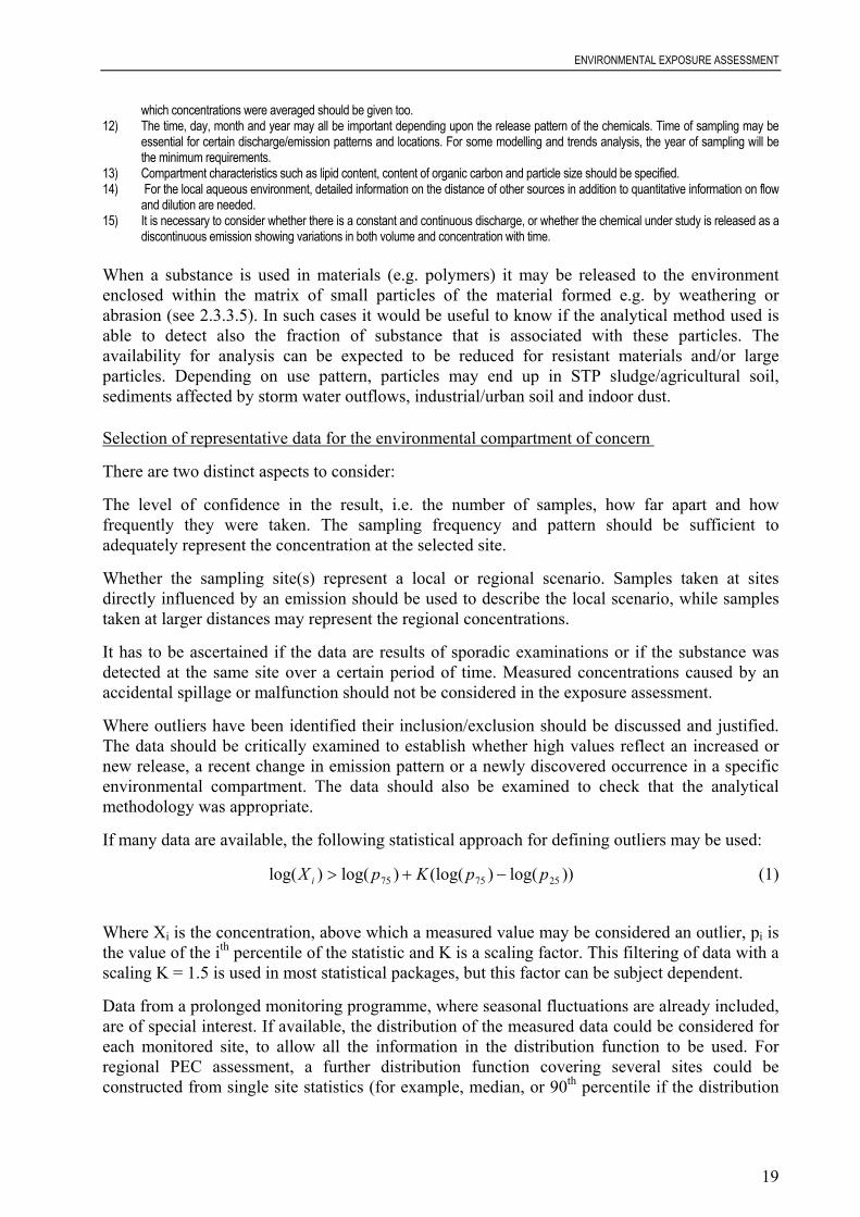
The structure of this section is shown schematically in Figure 2, including the flow of databetween the separate steps of the calculations.
D ata set2.3 .2
C om parison to (Q )SA R estim ationsC hapter 4
Sew age T reatm ent2.3 .7
R elease estim ation2.3 .3
R egional distr ibution2.3 .8 .7
A irA gricultura l soil
N atural soilIndustria l soil
Sedim entS urface w ater
S uspended matter
L ocal distr ibution2.3 .8 .1
A ir2 .3 .8 .2
S oil2 .3 .8 .5
G roundw ater2 .3 .8 .6
S urfaceW ater2 .3 .8 .3
Sedim ent2 .3 .8 .4
P artition coeffic ients2.3 .5
degra dation rates2.3 .6
C haracterisa tion ofthe environm ent
2 .3 .4
Figure 2 Lay out of section 2.3, including the flow of data between the different sections

ENVIRONMENTAL EXPOSURE ASSESSMENT
23
The model calculations are given in each section. The following table format is used forexplaining the symbols used in an equation:
Explanation of symbols
[Symbol] [Description of required parameter] [Unit] [Default value, equation numberwhere this parameter is calculated, or
[Symbol] [Description of resulting parameter] [Unit] reference to a table with defaults]
The following conventions are applied where possible for the symbols
• parameters are mainly denoted in capitals;• specification of the parameter is done in lower case;• specification of the compartment for which the parameter is specified is shown in subscripts.
Some frequently occurring symbols
E for emissions (direct and indirect) [kg.d-1]F for dimensionless fractions [kg.kg-1] or [m3.m-3]C for the concentration of a substance [mg.l-1], [mg.kg-1] or [mg.m-3]RHO for densities of compartments or phases [kg.m-3]K for intermedia partitioning coefficients [various units apply]k for (pseudo) first-order rate constants [d-1]T for a period of time [d]
As an example, the symbol Focsoil means the fraction (F) organic carbon (oc) in the soilcompartment (soil). For other parameters, recognisable symbols are chosen. It should be notedthat in several equations fixed factors (e.g. 1000 or 106) are applied for dimensional consistency.
Sensitivity analysis
In the case of conflicting data, great variation or uncertainty in data, a few carefully selectedscenarios could be considered employing alternative input parameters for the fate-relatedproperties in question. The fate-related properties may include data for bioaccumulation,sorption, degradation, volatilisation etc. The concept may also be useful for emissions if they areuncertain in relation to their size to certain environmental compartments.
However “the best value” according to the “realistic worst case” should be used in the “coreassessment”, and the alternative input values should only be included in alternative estimationsperformed for investigation purposes. It should be noted that fixing a parameter, which results ine.g. a higher PEC/PNEC ratio for sediment, soil, secondary poisoning and STP, will result in alower PEC/PNEC ratio for pelagic organisms. Therefore, in such cases it is possible that oneparticular set of parameters will give rise to the highest risk for one compartment, and anotherset for another compartment; both might be valid extremes.
The approach described above should especially be considered in relation to multi-componentsubstances / groups of substances where the intrinsic properties vary between the differentcomponents of the substance. It is important to know which components any measured valuesrelate to. The concept may, however, also be useful for certain discrete substances, where thereis special uncertainty about a fate related property or an emission that may be of key importance.
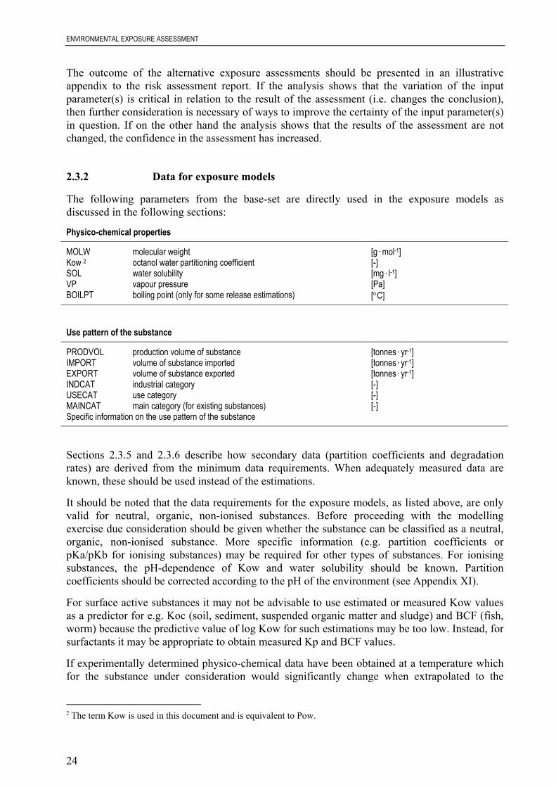
ENVIRONMENTAL EXPOSURE ASSESSMENT
24
The outcome of the alternative exposure assessments should be presented in an illustrativeappendix to the risk assessment report. If the analysis shows that the variation of the inputparameter(s) is critical in relation to the result of the assessment (i.e. changes the conclusion),then further consideration is necessary of ways to improve the certainty of the input parameter(s)in question. If on the other hand the analysis shows that the results of the assessment are notchanged, the confidence in the assessment has increased.
2.3.2 Data for exposure models
The following parameters from the base-set are directly used in the exposure models asdiscussed in the following sections:
Physico-chemical properties
MOLW molecular weight [g.mol-1]Kow 2 octanol water partitioning coefficient [-]SOL water solubility [mg.l-1]VP vapour pressure [Pa]BOILPT boiling point (only for some release estimations) [°C]
Use pattern of the substance
PRODVOL production volume of substance [tonnes.yr-1]IMPORT volume of substance imported [tonnes.yr-1]EXPORT volume of substance exported [tonnes.yr-1]INDCAT industrial category [-]USECAT use category [-]MAINCAT main category (for existing substances) [-]Specific information on the use pattern of the substance
Sections 2.3.5 and 2.3.6 describe how secondary data (partition coefficients and degradationrates) are derived from the minimum data requirements. When adequately measured data areknown, these should be used instead of the estimations.
It should be noted that the data requirements for the exposure models, as listed above, are onlyvalid for neutral, organic, non-ionised substances. Before proceeding with the modellingexercise due consideration should be given whether the substance can be classified as a neutral,organic, non-ionised substance. More specific information (e.g. partition coefficients orpKa/pKb for ionising substances) may be required for other types of substances. For ionisingsubstances, the pH-dependence of Kow and water solubility should be known. Partitioncoefficients should be corrected according to the pH of the environment (see Appendix XI).
For surface active substances it may not be advisable to use estimated or measured Kow valuesas a predictor for e.g. Koc (soil, sediment, suspended organic matter and sludge) and BCF (fish,worm) because the predictive value of log Kow for such estimations may be too low. Instead, forsurfactants it may be appropriate to obtain measured Kp and BCF values.
If experimentally determined physico-chemical data have been obtained at a temperature whichfor the substance under consideration would significantly change when extrapolated to the
2 The term Kow is used in this document and is equivalent to Pow.
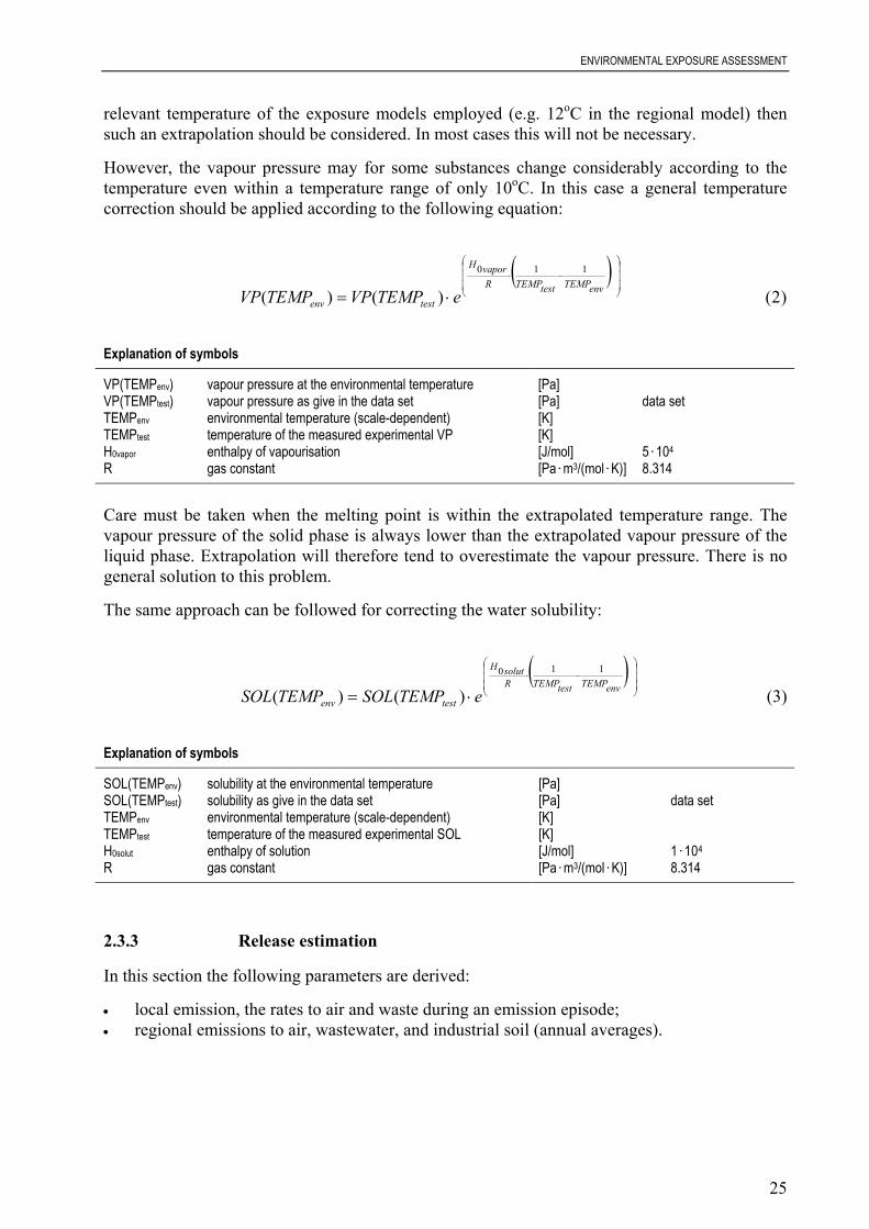
ENVIRONMENTAL EXPOSURE ASSESSMENT
25
relevant temperature of the exposure models employed (e.g. 12oC in the regional model) thensuch an extrapolation should be considered. In most cases this will not be necessary.
However, the vapour pressure may for some substances change considerably according to thetemperature even within a temperature range of only 10oC. In this case a general temperaturecorrection should be applied according to the following equation:
( )
−⋅
⋅= envTEMPtestTEMPRvaporH
testenv eTEMPVPTEMPVP
110
)()( (2)
Explanation of symbols
VP(TEMPenv) vapour pressure at the environmental temperature [Pa]VP(TEMPtest) vapour pressure as give in the data set [Pa] data setTEMPenv environmental temperature (scale-dependent) [K]TEMPtest temperature of the measured experimental VP [K]H0vapor enthalpy of vapourisation [J/mol] 5.104
R gas constant [Pa.m3/(mol.K)] 8.314
Care must be taken when the melting point is within the extrapolated temperature range. Thevapour pressure of the solid phase is always lower than the extrapolated vapour pressure of theliquid phase. Extrapolation will therefore tend to overestimate the vapour pressure. There is nogeneral solution to this problem.
The same approach can be followed for correcting the water solubility:
( )
−⋅
⋅= envTEMPtestTEMPRsolutH
testenv eTEMPSOLTEMPSOL
110
)()( (3)
Explanation of symbols
SOL(TEMPenv) solubility at the environmental temperature [Pa]SOL(TEMPtest) solubility as give in the data set [Pa] data setTEMPenv environmental temperature (scale-dependent) [K]TEMPtest temperature of the measured experimental SOL [K]H0solut enthalpy of solution [J/mol] 1.104
R gas constant [Pa.m3/(mol.K)] 8.314
2.3.3 Release estimation
In this section the following parameters are derived:
• local emission, the rates to air and waste during an emission episode;• regional emissions to air, wastewater, and industrial soil (annual averages).
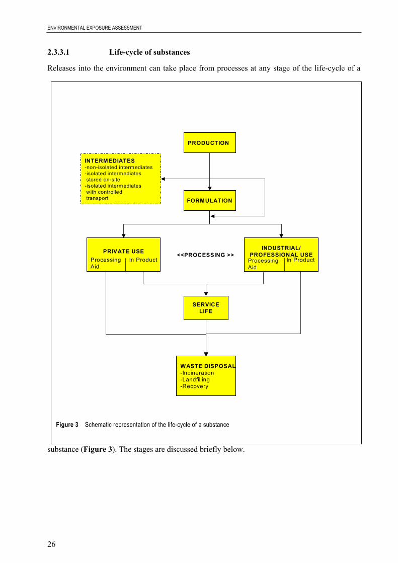
ENVIRONMENTAL EXPOSURE ASSESSMENT
26
2.3.3.1 Life-cycle of substances
Releases into the environment can take place from processes at any stage of the life-cycle of a
substance (Figure 3). The stages are discussed briefly below.
PRODUCTION
FORMULATION
PRIVATE USE INDUSTRIAL/PROFESSIONAL USE
WASTE DISPOSAL-Incineration-Landfilling-Recovery
INTERMEDIATES-non-isolated intermediates-isolated intermediates stored on-site
-isolated intermediates with controlledtransport
SERVICELIFE
<<PROCESSING >>ProcessingAid
In Product ProcessingAid
In Product
Figure 3 Schematic representation of the life-cycle of a substance
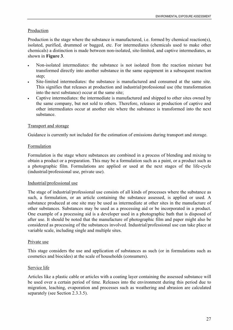
ENVIRONMENTAL EXPOSURE ASSESSMENT
27
Production
Production is the stage where the substance is manufactured, i.e. formed by chemical reaction(s),isolated, purified, drummed or bagged, etc. For intermediates (chemicals used to make otherchemicals) a distinction is made between non-isolated, site-limited, and captive intermediates, asshown in Figure 3.
• Non-isolated intermediates: the substance is not isolated from the reaction mixture buttransformed directly into another substance in the same equipment in a subsequent reactionstep;
• Site-limited intermediates: the substance is manufactured and consumed at the same site.This signifies that releases at production and industrial/professional use (the transformationinto the next substance) occur at the same site;
• Captive intermediates: the intermediate is manufactured and shipped to other sites owned bythe same company, but not sold to others. Therefore, releases at production of captive andother intermediates occur at another site where the substance is transformed into the nextsubstance.
Transport and storage
Guidance is currently not included for the estimation of emissions during transport and storage.
Formulation
Formulation is the stage where substances are combined in a process of blending and mixing toobtain a product or a preparation. This may be a formulation such as a paint, or a product such asa photographic film. Formulations are applied or used at the next stages of the life-cycle(industrial/professional use, private use).
Industrial/professional use
The stage of industrial/professional use consists of all kinds of processes where the substance assuch, a formulation, or an article containing the substance assessed, is applied or used. Asubstance produced at one site may be used as intermediate at other sites in the manufacture ofother substances. Substances may be used as a processing aid or be incorporated in a product.One example of a processing aid is a developer used in a photographic bath that is disposed ofafter use. It should be noted that the manufacture of photographic film and paper might also beconsidered as processing of the substances involved. Industrial/professional use can take place atvariable scale, including single and multiple sites.
Private use
This stage considers the use and application of substances as such (or in formulations such ascosmetics and biocides) at the scale of households (consumers).
Service life
Articles like a plastic cable or articles with a coating layer containing the assessed substance willbe used over a certain period of time. Releases into the environment during this period due tomigration, leaching, evaporation and processes such as weathering and abrasion are calculatedseparately (see Section 2.3.3.5).
ENVIRONMENTAL EXPOSURE ASSESSMENT
28
Waste disposal (including waste treatment and recovery)
At the end of the service life, the substance or a product containing the substance enters into thewaste disposal stage with waste or wastewater (Figure 4). Waste treatment may includeincineration or removal to landfill.
At this stage recovery processes may be applied. These usually involve a homogenisation and/orseparation step (e.g. mechanical treatment) followed by recovery of the targetsubstance/material. The recovered substance or material may be:
• reprocessed for the original type of product (recycling);• manufactured into a new type of product;• used as secondary fuel in heat production.
In the first option the substance returns into life-cycle stages already assessed before. In thesecond and third option the substance may enter into processing and final products from whichnew types and amounts of releases could occur. Whether or not these releases could be relevantto consider a case-by-case assessment. Some general criteria are given in Section 2.3.7.2.
In some cases, another substance or product may be recycled, and the substance assessed ispresent in this product. Releases in this situation may vary widely and information on them maynot be readily available since the focus of attention is not on the substance assessed, but on thesubstance or product recovered.
A substance present in a photographic bath for example, will be released at discharge after silverrecovery, and a substance present in printing ink will be released with wastewater and de-inkingsludge at paper recycling.
Releases from prolonged use of a product or articles in new applications after first service life(e.g. tyres in agriculture) without a waste specific treatment step in between should be assessedas a separate use in the relevant life-cycle stages i.e. processing/service, as appropriate.
In addition to being incinerated or being disposed of in landfill, waste may be released, eitherintentionally or unintentionally, to the environment. Articles may intentionally be left in theenvironment after their service life (e.g. cables buried in soil). Demolished building materialsmay be used as ballast at e.g. road constructions. Fragments of articles may also be lost duringuse (e.g. paint flakes, car undercoating).

ENVIRONMENTAL EXPOSURE ASSESSMENT
29
2.3.3.2 Types of emissions and sources
Emission patterns vary widely from well-defined point sources (single or multiple) to diffusereleases from large numbers of small point sources (like households) or line sources (like amotorway with traffic emissions). Releases may also be continuous or intermittent. Continuousemissions are characterised by an almost constant emission rate flow over a prolonged period(e.g. the emission of a substance from a continuous production process such as an oil refinery).Intermittent emissions can be peak emissions or block emissions (see Section 2.3.3.4). Peakemissions are characterised by a relatively large amount discharged in a short time where thetime intervals between peaks and the peak height can vary greatly (e.g. the discharge of spentliquid - reaction mixture - after isolation of the synthesised substance in a batch process). Blockemissions are characterised by a flow rate which is reasonably constant over certain time periodswith regular intervals with a low or even zero background emission (e.g. the emissions fromtraffic during the day; during rush hours emission are particularly high). The quantities releasedfrom a certain process may vary from 100%, as is the case for example with household productslike detergents or volatile solvents in paints, to below 1% for substances like intermediatesproduced in closed systems.
Product at end of service life
Collected waste
Mechanical treatment
Recycling Co-incineration or other recovery
Waste incineration
Landfill
Industrial product (e.g.
cement)
Use of residues in products
Waste remaining in the environment
Back to processing
WASTE SCENARIOS
Figure 4 Schematic representation of the waste life stage of a substance
ENVIRONMENTAL EXPOSURE ASSESSMENT
30
Besides releases from point sources, diffuse emissions from articles during their service life maycontribute to the total exposure for a substance. For substances used in long-life materials thismay be a major source of emissions (both during use and as waste remaining in the environment,see Section 2.3.3.5).
Emissions related to the waste life stage can take place several decades after production andprocessing of a substance. They may follow the market volume of the substance with a delayspecific for a certain type of product. Emission patterns (e.g. route, quantity and trend in time)may also be determined by the type of treatment in relation to substance properties. Little isknown of the magnitude of long-term releases, e.g. of metals or of organic substances that do notdegrade anaerobically (see Section 2.3.3.6).
2.3.3.3 Release estimation
It is clear that the releases of a substance are dependent on the use patterns. Three categories aredistinguished, i.e. main category, industry category and function or use category. An overview ofthese categories can be found in Chapter 5. The main categories are intended to describegenerally the exposure relevance of the use(s) of a substance. In the context of environmentalrisk assessment they are also used to characterise release scenarios for the estimation ofemissions to the environment during specific stages of the life-cycle of the substance(production, formulation, and industrial/professional use). They can therefore be allocated torelease fractions, which are used as default values where specific information is missing. Thefollowing Main Categories are distinguished:
• use in closed systems: refers to the industrial/professional use stage when a substance is used forexample in a transformer or a circulation circuit of a refrigerator, or it may refer to the stage ofproduction where a substance like an intermediate is manufactured in closed apparatus;
• use resulting in inclusion into or onto a matrix: refers to the stage of formulation, e.g. whena substance is included in the emulsion layer of a photographic film. It also may refer to thestage of industrial/professional use, e.g. when a substance, applied as a uv-stabiliser in paint,ends up in the finished coating layer;
• non-dispersive use: relates to the number (and size) of the emission sources;• wide dispersive use: relates also to the number (and size) of the emission sources.
The industry categories specify the branch of industry (including personal and domestic use, anduse in the public domain) where considerable emissions occur by application of the substance assuch, or by the application and use of preparations and products containing the substance. Someimportant emission sources have not been included specifically in this scheme and hence have tobe allocated to category “Others” (no. 15/0), e.g. emissions of substances (in preparations) otherthan fuels and fuel additives used in motor vehicles.
The use or function category specifies the specific function of the substance. There are 55categories which have a varying level of detail. For substances used in photography for example,there is only one category: 42 “Photochemicals”. Depending on the specific function of thephotochemical, however, emissions can vary to a great extent, e.g. substances used to influencethe crystal growth of silver compounds at the production of films are released by over 50%,while other substances at this stage will hardly be released. There is no general category as“Plastics additives” and many other specific categories lack as well; exceptions are categorieslike 47 “Softeners” (= plasticisers) and 49 “Stabilisers” (heat and UV-stabilisers).

ENVIRONMENTAL EXPOSURE ASSESSMENT
31
The release of a substance at different stages of its life-cycle should be estimated by order ofpreference from:
1. specific information for the given substance (e.g. from producers, product registers or openliterature);
2. specific information from the emission scenario documents (use category documents) forseveral industrial categories as well as for some of the 23 biocidal Product Types as given inPart IV, Chapter 7;
3. emission factors as included in the release tables of Appendix I.
Emissions may occur from a category other than the one to which a substance is allocated. Asubstance used in paint will normally be allocated to category 14 “Paints, lacquers and varnishes”.Though the local emissions of solvents may be considerable at one point source (the paint factory)at the stage of formulation (paint production), most of the solvent will be emitted at paintapplication. The application could be classified in several industrial categories depending on thetype of paint. In case of a do-it-yourself paint it would belong to category 5 “Personal/domestic”, incase of motor car repair or professional house painting it would be category 15/0 “Others” (widedispersive use, so diffuse releases) and in case of motor car production 16 “Engineering industry:civil and mechanical” (non-dispersive use, so few large point sources).
It is possible that confusion arises when the use of a substance, belonging to a certain specificprocess of an industrial category, occurs at another branch of industry. One example is theapplication of an additive for an epoxy resin applied in the electronic industry for the embeddingof electronic components. Though the industrial/professional use takes place at category 4“Electrical/electronic engineering industry” the industrial/professional use of epoxy resinsbelongs to category 11 “Polymers industry”. The releases from the process will be found in thetable for the latter category. Further information on main categories, industry categories and usecategories is provided in Appendix I, together with more examples.
For chemical industry, two separate industrial categories exist, one for basic chemicals andanother for chemicals used in synthesis. Basic chemicals are considered to comprise commonlyused chemicals such as solvents and pH-regulating agents such as acids and alkalis. Also theprimary chemicals from the oil refining process are considered as basic chemicals. Substancesused in synthesis fall in two classes, namely intermediates (substances produced from a startingmaterial to be converted in a subsequent reaction into a next substance) and other substances.These other substances consist mainly of 'process regulators' (e.g. accelerators, inhibitors,indicators). For industrial category 5 (personal/domestic) the use and application of substances(as such or in formulations) is considered at the scale of households. The types of application aree.g. adhesives, cosmetics, detergents, and pharmaceuticals. Some applications have been coveredin other industrial categories at the stage of private use. These applications comprise fuels andfuel additives (mineral oil and fuel industry), paint products (paints, lacquers and varnishesindustry) and photochemicals (photographic industry). For industrial category 6 (public domain),use and application at public buildings, streets, parks, offices, etc. is considered.
The A-tables of Appendix I provide the estimated total release fractions of the productionvolume (emission factors) to air, (waste) water and industrial soil during production,formulation, industrial/professional use, private use, and recovery, according to their industrialcategory. The production volume is defined as the total tonnage of a substance brought to theEuropean market in one year, i.e. the total volume produced in the EU plus the total amountimported into the EU, and minus the total volume exported from the EU excluding the volume of

ENVIRONMENTAL EXPOSURE ASSESSMENT
32
the substance present in products imported/exported. The total volume released is averaged overthe year and used for the PECregional calculation.
The B-tables of Appendix I are used for the determination of the releases from point sources forthe evaluation of PEClocal. They provide the fraction of the total volume released that can beassumed to be released through a single point source, and the number of days during which thesubstance is released, thus allowing the daily release rate at a main point source to be calculated.
Despite the need for applying expert judgement when determining the fraction of main source,the following general guidelines for the emission estimation should be applied:
• for production the input for the regional production volume is by default set at the EUproduction volume, which is also used as input for the B-tables. Based on the informationavailable to the rapporteur on the number of production sites, size distribution and geographicdistribution it can be decided to apply a 10% rule, where it is assumed that 10% of the amountthat is produced and used in the EU is produced/used within a region and it is subsequentlyassumed that the size of the main local source can be obtained by multiplying this amount withthe fraction of main source from the B-tables. Alternatively it can be decided to use anotherpercentage or to use specific values as input for the regional model (e.g. the emissions from thelargest source or the emissions from the largest emitter) where this reflects a more realisticworst case. Similarly this information can be used to set the fraction of main source for thelocal exposure calculation. It should be noted that if site-specific data are available then it canbe the case that the largest site is not the largest source of emissions;
• for formulation and processing (industrial use) a similar approach as for production is used:by default the EU volume is used as input for the region as well as for the B-tables unless itcan be shown/is known that a large number of sites with a reasonable European distributionexists for the specific formulation/processing step of the substance involved. In that caseagain it can be decided to apply the 10% rule, to use another percentage or to use specificvalues. Whether or not the available information is sufficient for a specific substance willdepend on the expert judgement by the rapporteur;
• for private use the 10% rule is applied by default both for the input of the regional volumeand for the input volume for the B-table in agreement with the assumption of 10% of the useoccurring in the region.
It must be realised that depending on the IC/UC combination this approach may in some caseslead to unreasonable worst-case assumptions, especially for the estimation of the emissionsduring formulation/processing. Hence, a case-by-case assessment using expert judgementremains warranted. For new substances the default should be overwritten anyway because it maybe assumed that in most cases just one or at the most a few producers exist.
To obtain the best entry to the tables for emission factors, Appendix I also contains a list ofsynonyms for functions of substances. The synonyms and their definitions have been derivedfrom the US EPA ChemUSES list (US EPA, 1980).
In general, the data supplied by industry will help to find the correct entry to the release tablesapart from the classification specified in Chapter 5.
The production volume is expressed in tonnes/year in the data set and denoted by PRODVOL.TONNAGE is the volume of substance that is used for subsequent life-cycle stages. In the emissiontables of Appendix IB, PRODVOL must be used for T when estimating releases at productionwhereas TONNAGE should be used as T for the subsequent life-cycle stages. If at the disposal
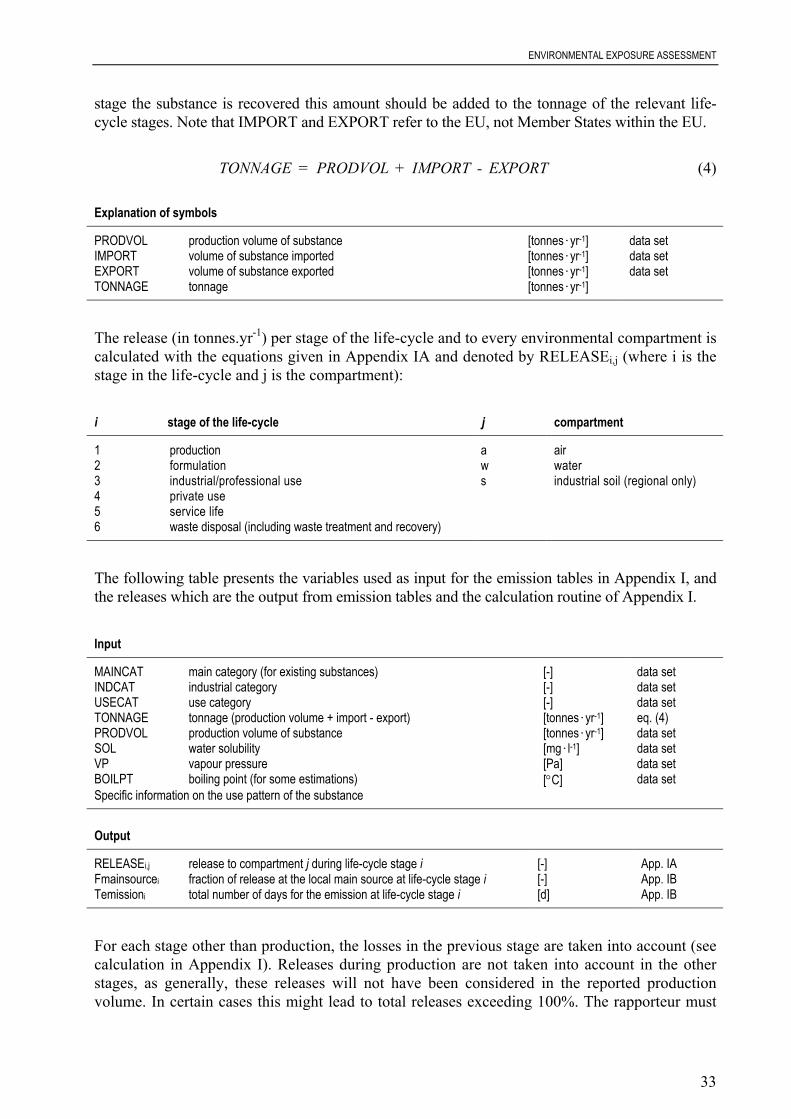
ENVIRONMENTAL EXPOSURE ASSESSMENT
33
stage the substance is recovered this amount should be added to the tonnage of the relevant life-cycle stages. Note that IMPORT and EXPORT refer to the EU, not Member States within the EU.
TONNAGE = PRODVOL + IMPORT - EXPORT (4)
Explanation of symbols
PRODVOL production volume of substance [tonnes.yr-1] data setIMPORT volume of substance imported [tonnes.yr-1] data setEXPORT volume of substance exported [tonnes.yr-1] data setTONNAGE tonnage [tonnes.yr-1]
The release (in tonnes.yr-1) per stage of the life-cycle and to every environmental compartment iscalculated with the equations given in Appendix IA and denoted by RELEASEi,j (where i is thestage in the life-cycle and j is the compartment):
i stage of the life-cycle j compartment
1 production a air2 formulation w water3 industrial/professional use s industrial soil (regional only)4 private use5 service life6 waste disposal (including waste treatment and recovery)
The following table presents the variables used as input for the emission tables in Appendix I, andthe releases which are the output from emission tables and the calculation routine of Appendix I.
Input
MAINCAT main category (for existing substances) [-] data setINDCAT industrial category [-] data setUSECAT use category [-] data setTONNAGE tonnage (production volume + import - export) [tonnes.yr-1] eq. (4)PRODVOL production volume of substance [tonnes.yr-1] data setSOL water solubility [mg.l-1] data setVP vapour pressure [Pa] data setBOILPT boiling point (for some estimations) [°C] data setSpecific information on the use pattern of the substance
Output
RELEASEi,j release to compartment j during life-cycle stage i [-] App. IAFmainsourcei fraction of release at the local main source at life-cycle stage i [-] App. IBTemissioni total number of days for the emission at life-cycle stage i [d] App. IB
For each stage other than production, the losses in the previous stage are taken into account (seecalculation in Appendix I). Releases during production are not taken into account in the otherstages, as generally, these releases will not have been considered in the reported productionvolume. In certain cases this might lead to total releases exceeding 100%. The rapporteur must

ENVIRONMENTAL EXPOSURE ASSESSMENT
34
specify if releases during each stage are relevant or not. If the release during a certain life stageis not applicable, the release fraction will be set to zero.
Furthermore, few quantitative methods have been developed for estimation of the emissionsduring the service life of articles containing the substance (main category II) e.g. for emission ofa flame retardant in plastics used for TV-sets, radios etc. However, though quantitativemethodologies are at present scarce for these types of emissions, preliminary quantitativeestimations may be performed on a case-by-case basis (see Section 2.3.3.5).
After accounting for losses during the six stages of the life-cycle, the part of the tonnage thatremains is assumed to end up in waste streams completely. Quantitative methods for estimatingemissions at the disposal stage are currently available for municipal waste incineration andmunicipal landfills. However, at present there is not sufficient information available, to set up anemission scenario which is representative at EU level. Nevertheless, preliminary quantitativeestimations modelling a reasonable worst case for the regional scenario may be performed on acase-by-case basis. Quantitative methods for the various types of waste operations aiming atrecovery are at the stage of development. Preliminary quantitative estimations may be performedon a case-by-case basis (see Sections 2.3.3.6 and 2.3.7.2).
For local emissions for every environmental compartment, the main point source and each stage ofthe life-cycle is considered. The emission rate is given averaged per day (24 hours). This impliesthat, even when an emission only takes place a few hours a day, the emission will be averaged over24 hours. Emissions to air and water will be presented as release rates during an emission episode.Local emissions can be calculated for each stage of the life-cycle and each compartment:
i, j ii
i, jElocal = Fmainsource Temission
RELEASE• •1000 (5)
Explanation of symbols
RELEASEi,j release during life-cycle stage i to compartment j [tonnes.yr-1] App. IAFmainsourcei fraction of release at the local main source at life-cycle stage i [-] App. IBTemissioni number of days per year for the emission in stage i [d.yr-1] App. IBElocali,j local emission during episode to compartment j during stage i [kg.d-1]
For local release estimates, point sources (and therefore, presumably single stages of the life-cycle) need to be identified. It will normally be necessary to assess each stage of the life-cycle todetermine whether adverse effects can occur since decisions need to be made to clarify or reduceany identified risk for all life-cycle stages. This is not required if it is obvious that a certain stageis negligible.
For the regional scale assessments, the release fractions for each stage of the life-cycle need tobe summed for each compartment. The emissions are assumed to be a constant and continuousflux during the year. Regional emissions can be calculated as:
∑=
•6
1,365
1000i
jij RELEASE = Eregional (6)

ENVIRONMENTAL EXPOSURE ASSESSMENT
35
Explanation of symbols
RELEASEi,j release during life-cycle stage i to compartment j [tonnes.yr-1] App. IAEregionalj total emission to compartment j (annual average) [kg.d-1]
When assessing the releases on local and regional scales, the following points must be noted:
• in particular High Production Volume Chemicals (HPVCs) often have more than oneapplication, sometimes in different industrial categories. For these substances, theassessment proceeds by breaking down the production volume for every applicationaccording to data from industry. For the local situation, in principle, all stages of the life-cycle need to be considered for each application. Where more than one stage of the life-cycle occurs at one location, the PEClocal shall be calculated by summing all the relevantemissions from that location. For releases to wastewater, only one point source for the localSTP is considered. For the regional situation, the emissions to each compartment have to besummed for each stage of the life-cycle and each application. The regional environmentalconcentrations are used as background concentrations for the local situation;
• if substances are applied in products with an average life span of many years, after the initialarrival of the products onto the market the yearly emissions to the environment willincrease. However, after a certain number of years with similar use of the products a steady-state situation will be reached. Examples are a plastic article or a paint coating where thesubstance assessed is applied as a plasticiser (see also Section 2.3.3.5).
Emission reduction techniques have not been taken into account in the tables of Appendix IA asthe kind of techniques applied (with possibly large differences in efficiencies) as well as thedegree of penetration may differ between Member States or industry sectors. Only when for acertain process a specific reduction measure is common practice this will be taken into account.In all other cases, reasonable worst-case applies.
2.3.3.4 Intermittent releases
Many substances are released to the environment from industrial sources as a result of batch,rather than continuous, processes. In extreme cases, substances may only be emitted a few timesa year. Since the PECs associated with industrial releases can take into account both the amountreleased and the number of days of emission, the magnitude of the PECs in the risk assessmentshould not be affected. PEClocal is always calculated on the basis of a daily release rate,regardless of whether the discharge is intermittent or continuous. It represents the concentrationexpected at a certain distance from the source on a day when discharge occurs. The discharge isalways assumed to be continuous over the 24-hour period. On the other hand, PECregional iscalculated using the annual release rate. It represents the steady-state concentration to beexpected, regardless of when the discharge occurred.
Intermittent release needs to be defined, although rapporteurs will have to justify the use of thisscenario on a case-by-case basis. Intermittent release can be defined as “intermittent but onlyrecurring infrequently i.e. less than once per month and for no more than 24 hours”.
This would correspond to a typical batch process only required for a short period of the year(releases to the environment may be only of limited duration). Thus, for the aquaticcompartment, transport processes may ensure that the exposure of aquatic organisms is of shortduration. Calculation of the likely exposure period should take into account the potential of asubstance to substantially partition to the sediment. Such partitioning, while reducing the

ENVIRONMENTAL EXPOSURE ASSESSMENT
36
calculated PEClocalwater may also increase the exposure time by repartitioning to the water phaseover an extended period. For intermittent releases to the aquatic compartment a dedicated PNECis used in the risk characterisation (see Section 3.2.2) that has been derived using a methoddiffering from the usual one.
Where the batch process occurs more frequently than above or is of a longer duration, protectionagainst short-term effects cannot be guaranteed because fish, rooted plants and the majority ofthe macro-invertebrates are more likely to be exposed to the substance on the second andsubsequent emissions. When intermittent release is identified for a substance, this is notnecessarily applicable to all releases during the life-cycle.
2.3.3.5 Emissions during service-life of long-life articles
Long-life articles are here defined as articles having a service-life longer than one year.Substances in such articles may accumulate in society (landfills excluded). The emissions fromlong-life articles can be expected to be highest at steady state (i.e. when the flow of an articleinto society equals the outflow, see Figure 5). Estimating the emissions often requiresknowledge of the substance use pattern in the preceding years.
There are several mechanisms for diffuse emission such as evaporation, leaching, corrosion,abrasion and weathering effects. An additional release route that in some cases is of importanceis when a substance diffuses from one material into another (e.g. from glue material intoconstruction material). Substances that are slowly emitted from long-life materials are oftencharacterised by inherent properties such as low water solubility and low vapour pressure (e.g.
Inc in e ra tio ns ites
La ndfills
C O N T I N E N T A L / R E G I O N A L S C A L E
A ccu m u la ted am o u n t o f su b s tan ce X in th e so c iety
A
S TP
A n n u al in pu t f rom "pro du c tion ", "form u lation " an d “ in du s trial/ profess ion al
u se”
E xp la na t io n o f s ym bo ls : A nnua l f lo w o f s ubs ta nce X in m o lec u la r fo rm
A nnua l f lo w o f s ubs ta nce X in fo rm o f a rtic les /m a te ria ls
C
L O C A L S C A L E
E
G
I
F
H
K
A cc um ulate d am o un t o f s u bs ta nce X in "w aste rem ainin g in th e e nviro nm e nt"
U R B A N /IN D .S O IL
S U R FA C EW A TE R
A IR
J K
B D
Figure 5 Emissions from long-life articles at Steady state (A = B + C + D + E + F + G + H for society ; H = I + J + K for “waste remaining in the environment”).
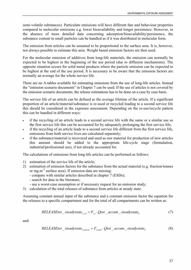
ENVIRONMENTAL EXPOSURE ASSESSMENT
37
semi-volatile substances). Particulate emissions will have different fate and behaviour propertiescompared to molecular emissions e.g. lower bioavailability and longer persistence. However, inthe absence of more detailed data concerning adsorption/bioavailability/persistence, thesubstance content in small particles can be handled as if it was distributed in molecular form.
The emission from articles can be assumed to be proportional to the surface area. It is, however,not always possible to estimate this area. Weight based emission factors are then used.
For the molecular emission of additives from long-life materials, the emission can normally beexpected to be highest in the beginning of the use period (due to diffusion mechanisms). Theopposite situation occurs for solid metal products where the particle emission can be expected tobe highest at the end of the use period. It is necessary to be aware that the emission factors arenormally an average for the whole service life.
There are no A-tables available for estimating emissions from the use of long-life articles. Insteadthe “emission scenario documents” in Chapter 7 can be used. If the use of articles is not covered bythe emission scenario documents, the release estimations has to be done on a case by case basis.
The service life of an article can be defined as the average lifetime of the article. If a significantproportion of an article/material/substance is re-used or recycled leading to a second service lifethis should be considered in the exposure assessment. Depending on the re-use/recycle patternthis can be handled in different ways:
• if the recycling of an article leads to a second service life with the same or a similar use asthe first service life this can be accounted for by adequately prolonging the first service life;
• if the recycling of an article leads to a second service life different from the first service life,emissions from both service lives are calculated separately;
• if the substance/material is recovered and used as raw material for production of new articlesthis amount should be added to the appropriate life-cycle stage (formulation,industrial/professional use), if not already accounted for.
The calculations of emissions from long-life articles can be performed as follows:
1) estimation of the service life of the article;2) estimation of emission factors for the substance from the actual material (e.g. fraction/tonnes
or mg.m-2 surface area). If emission data are missing:- compare with similar articles described in chapter 7 (ESDs);- search for data in the literature;- use a worst-case assumption or if necessary request for an emission study;
3) calculation of the total releases of substance from articles at steady state.
Assuming constant annual input of the substance and a constant emission factor the equation forthe releases to a specific compartment and for the total of all compartments can be written as:
kjikji esteadystataccumQtotFesteadystatRELEASEtot ___ ,,, ⋅= (7)
and:
ktotaliktotali esteadystataccumQtotFesteadystatRELEASEtot ___ ,,, ⋅= (8)

ENVIRONMENTAL EXPOSURE ASSESSMENT
38
where the amount accumulated in product k in the society at the end of service life (steady state)can be calculated as:
∑=
−−⋅=kTservice
y
yi,totalkk FQtotte_steadystaQtot_accum
1
1)1( (9)
In situations where the emission factor is low (< 1%.yr-1) and the service life of the product isnot very long, the emissions and accumulation at steady state (eq. 7-9) can be simplified as:
kkjikji TserviceQtotFesteadystatRELEASEtot ⋅⋅= ,,,_ (10)
kktotaliktotali TserviceQtotFesteadystatRELEASEtot ⋅⋅= ,,,_ (11)
kkk TserviceQtotesteadystataccumQtot ⋅=__ (12)
Explanation of symbols
Fi,,j Fraction of tonnage released per year (emission factor)during life-cycle stage i (service life) to compartment j [-] data set 1)
Fi,total Fraction of tonnage released per year (emission factor)during life-cycle stage i (service life) to all relevantcompartments [-] data set 2)
RELEASEtot_steady statei,j,k Annual total release to compartment j at steady state for product k [tonnes.yr-1]
RELEASEtot_steady statei,total,k Annual total releases to all relevant compartmentsat steady state for product k [tonnes.yr-1]
Qtotk Annual input of the substance in product k [tonnes.yr-1] data setQtot_accum_steady statek Total quantity of the substance accumulated
in product k at steady state [tonnes]Tservicek Service life of product k [yr] data set
1) Alternatively use equation 162) Alternatively use equation 17
The annual total amount that will end up as waste from product k at the end of service life atsteady state (b+c+h in Figure 5) can be written as (assuming no degradation within the article):
ktotalikk esteadystatRELEASEtotQtotesteadystatQWASTEtot ,,__ −= (13)
Explanation of symbols
QWASTEtot_steady statek Total quantity of the substance in product k endingup as waste at steady state [tonnes.yr-1]
Qtotk Annual input of the substance in product k [tonnes.yr-1] data setRELEASEtot_steady statei ,total,k Annual total releases to all relevant compartments
at steady state for product k [tonnes.yr-1] eq. (8)
ENVIRONMENTAL EXPOSURE ASSESSMENT
39
Using a 10% default the annual regional release from article k to compartment j and for the totalof all compartments can be calculated as:
1.0__ ,,,, ⋅= kjikji esteadystatRELEASEtotesteadystatRELEASEreg (14)
and:
1.0__ ,,,, ⋅= ktotaliktotali esteadystatRELEASEtotesteadystatRELEASEreg (15)
Explanation of symbols
RELEASEreg_steady statei,j,k Annual regional release to compartment jat steady state for product k [tonnes.yr-1]
RELEASEreg_steady statei,total,k Annual regional release to all relevant compartmentsat steady state for product k
[tonnes.yr-1]RELEASEtot_steady statei,j,k Annual total release to compartment j
at steady state for product k [tonnes.yr-1] eq. (7/10)RELEASEtot_steady statei,total,k Annual total releases to all relevant compartments
at steady state for product k [tonnes.yr-1] eq. (8/11)
These regional diffuse releases are then added to the regional emissions calculated from non-diffuse emissions (Eregionalj; eq. (6))
If an emission factor is available as release per surface area, it can be converted to a productspecific “fraction of tonnage released” (Fi,j and Fi,total):
kk
kjiji CONC THICK
1000eaEMISSIONar specific)(product F ,,
, ∗
∗= (16)
and:
kk
ktotalitotali CONC THICK
1000eaEMISSIONar specific)(product F ,,
, ∗∗
= (17)
Explanation of symbols
Fi,j Fraction of tonnage released per year (emission factor) during lifecycle stage i (service life) to comparment j from product k [yr-1]
Fi,total Fraction of tonnage released per year (emission factor) during lifecycle stage i (service life) to all relevant compartments from product k [yr--1]
CONCk Concentration of substance in product k [kg.dm-3] data setEMISSIONareai,j,k Annual amount of substance emitted per area from product k
to compartment j [g.m-2.yr-1] data setEMISSIONareai,total,k Annual total of amount substance emitted per area from product k [g.m-2.yr-1] data setTHICKk Thickness of the emitting material in product k [mm] data set
If the area based emissions can be expected to decrease with decreasing concentration in theproduct the equations 7-8 above are used. If the emission is expected to be independent of the
ENVIRONMENTAL EXPOSURE ASSESSMENT
40
remaining amount of the substance in the product, e.g. corroding metals, the simplified equations10-11 are used.
If the amount of a substance in use in the society has not reached steady state and theaccumulation is still ongoing, the calculated PEC will represent a future situation. If this is thecase this should be considered when comparing PEC with monitoring data.
Releases from articles will normally only contribute to the continental and regional releases. Theemissions from indoor uses can be released to wastewater and therefore be regarded as a pointsource (stream “d” in Figure 5). Also outdoor uses may cause releases to STP if the storm watersystem is connected to the STP. This has to be considered case by case. For the calculation of alocal scenario the B-table in Appendix I for Industry Category 5 Personal/domestic shall be used.
Quantitative methods for estimating emissions from waste remaining in the environment arecurrently not available. Therefore such releases have to be considered on a case-by-case basis.As for substances in long-life articles, substances in “waste remaining in the environment” willalso accumulate. As a simplification the emissions at steady state can be assumed to be equal tothe annually formed amount of “waste remaining in the environment” (see Figure 5). If thedegradation rate of the substance in the waste material is known, this should be taken intoconsideration. When the emission of a substance from waste remaining in the environment isvery slow it will take a long time to reach steady state. In that case the calculated emission mayreflect a future situation.
As for emissions from articles releases from waste remaining in the environment will alsocontribute mainly to the continental and regional releases.
2.3.3.6 Emissions from waste disposal
If the major share of a substance placed on the market remains in chemical products or articles atthe end of their service life (releases during production, processing and use are comparativelysmall), the waste life-cycle stage of the substance may need particular attention. This refers e.g.to organic substances in landfills and metals in waste incineration processes. The underlyingcriterion for considering waste emissions in the risk assessment of substances, is that the wastestage will contribute significantly to the overall human exposure or environmental concentrationin comparison to the emissions from other parts of the life-cycle of the substance (e.g.production and use stages). If this is not the case, waste considerations could be excluded fromthe assessment process and general risk management measures based on EU waste legislationshould be sufficient.
For certain types of substances, e.g. metals and persistent and toxic substances releases fromwaste may be slow compared to the release from the production and use phase but neverthelessthe continued long-term release after use could be of concern. On a case-by-case basis, theseaspects may be addressed in the risk assessment.
To guide the decision whether an estimation of the releases from the waste stage is pertinent, thefollowing considerations may be used.
First, on the basis of the production volume and the use pattern a preliminary assessment on thevolume that may end up in the waste streams should be performed. In doing so the toxicity andother adverse effects of the substance and of possible breakdown products should be taken into
ENVIRONMENTAL EXPOSURE ASSESSMENT
41
account to qualify the significance of the possible impact of such a volume entering the wastestream. Even a small volume of a highly toxic compound may be of concern.
Subsequently, information on anaerobic degradation in landfills or conditions simulatingconditions in landfills may indicate that further assessment may not be needed. Water solubility,adsorption/desorption in soil (under landfill conditions) or if available from leachingexperiments could also be included in the evaluation as an indicator for leaching potential.However, it is noted that even sorbed substances may leave the landfill via particle transportwith leachates.
The substance may also leave the landfill with the produced landfill gas. The Kow and Henry’sLaw constant as well as the tropospheric persistency may be used to indicate whether the releasethrough landfill gas may be of significance. A proposal for possible trigger values can be foundin Danish EPA (2001).
For incineration, inorganic substances are the predominant substances of concern. The concern isespecially associated with possible leaching of such substances from incineration productswhether landfilled or used e.g. for road construction. Furthermore, substances that containhalogens need special attention due to the possible formation of hazardous substances duringincineration.
In order to evaluate whether emissions from incineration of a substance containing an inorganicsubstance of concern should be included in the risk assessment, the predicted occurrence of thesubstance in a waste stream should be compared with typical background-ranges. If a substanceor a specific use of a substance may contribute unduly to the influent concentration furtherrelease calculation should be carried out.
2.3.3.7 Delayed releases from waste disposal and dilution in time
Releases from the waste life stage may occur several decades after production and processing ofthe substance under assessment. These delays are determined, inter alia, by:
• the service life span of the substance as such, or in a chemical product or article;• intermediate storage after service life before waste collection (e.g. exhausted batteries);• exposure of residues from waste incineration to water. This source could be of particular
relevance if the residues are re-introduced into the market as products (e.g. buildingmaterial) exposed to water;
• intensity of gas production in landfills;• exposure of landfilled waste to water and deterioration of the landfill bottom liner.
The releases from landfills and residues from waste incineration residues usually take place overa long time period. Hence the daily or annual release may result in a very small PEC. Ifavailable, monitoring data may be a valuable source of information (see Section 2.2.1). The needfor a long-term release assessment should be decided on a case-by-case basis, in particular formetals or organic substances that are persistent and toxic.
2.3.4 Characterisation of the environmental compartments
In this section, the following parameters are derived:
• definition of the standard environmental characteristics (Table 5);

ENVIRONMENTAL EXPOSURE ASSESSMENT
42
• bulk densities for soil, sediment, and suspended matter.
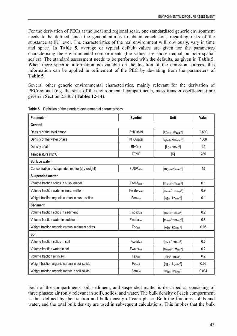
ENVIRONMENTAL EXPOSURE ASSESSMENT
43
For the derivation of PECs at the local and regional scale, one standardised generic environmentneeds to be defined since the general aim is to obtain conclusions regarding risks of thesubstance at EU level. The characteristics of the real environment will, obviously, vary in timeand space. In Table 5, average or typical default values are given for the parameterscharacterising the environmental compartments (the values are chosen equal on both spatialscales). The standard assessment needs to be performed with the defaults, as given in Table 5.When more specific information is available on the location of the emission sources, thisinformation can be applied in refinement of the PEC by deviating from the parameters ofTable 5.
Several other generic environmental characteristics, mainly relevant for the derivation ofPECregional (e.g. the sizes of the environmental compartments, mass transfer coefficients) aregiven in Section 2.3.8.7 (Tables 12-14).
Table 5 Definition of the standard environmental characteristics
Parameter Symbol Unit Value
General
Density of the solid phase RHOsolid [kgsolid.msolid-3] 2,500
Density of the water phase RHOwater [kgwater.mwater-3] 1000
Density of air RHOair [kgair.mair-3] 1.3
Temperature (12°C) TEMP [K] 285
Surface water
Concentration of suspended matter (dry weight) SUSPwater [mgsolid.lwater-1] 15
Suspended matter
Volume fraction solids in susp. matter Fsolidsusp [msolid3.msusp-3] 0.1
Volume fraction water in susp. matter Fwatersusp [mwater3.msusp-3] 0.9
Weight fraction organic carbon in susp. solids Focsusp [kgoc.kgsolid-1] 0.1
Sediment
Volume fraction solids in sediment Fsolidsed [msolid3.msed-3] 0.2
Volume fraction water in sediment Fwatersed [mwater3.msed-3] 0.8
Weight fraction organic carbon sediment solids Focsed [kgoc.kgsolid-1] 0.05
Soil
Volume fraction solids in soil Fsolidsoil [msolid3.msoil-3] 0.6
Volume fraction water in soil Fwatersoil [mwater3.msoil-3] 0.2
Volume fraction air in soil Fairsoil [mair3.msoil-3] 0.2
Weight fraction organic carbon in soil solids Focsoil [kgoc.kgsolid-1] 0.02
Weight fraction organic matter in soil solids Fomsoil [kgom.kgsolid-1] 0.034
Each of the compartments soil, sediment, and suspended matter is described as consisting ofthree phases: air (only relevant in soil), solids, and water. The bulk density of each compartmentis thus defined by the fraction and bulk density of each phase. Both the fractions solids andwater, and the total bulk density are used in subsequent calculations. This implies that the bulk
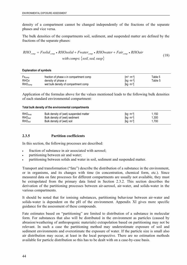
ENVIRONMENTAL EXPOSURE ASSESSMENT
44
density of a compartment cannot be changed independently of the fractions of the separatephases and vice versa.
The bulk densities of the compartments soil, sediment, and suspended matter are defined by thefractions of the separate phases:
{ }susp sed,soil, comp withRHOairFairRHOwaterFwaterRHOsolidFsolidRHO compcompcompcomp
∈
++= ••• (18)
Explanation of symbols
Fxcomp fraction of phase x in compartment comp [m3.m-3] Table 5 RHOx density of phase x [kg.m-3] Table 5RHOcomp wet bulk density of compartment comp [kg.m-3]
Application of the formulas above for the values mentioned leads to the following bulk densitiesof each standard environmental compartment:
Total bulk density of the environmental compartments
RHOsusp Bulk density of (wet) suspended matter [kg.m-3] 1,150RHOsed Bulk density of (wet) sediment [kg.m-3] 1,300RHOsoil Bulk density of (wet) soil [kg.m-3] 1,700
2.3.5 Partition coefficients
In this section, the following processes are described:
• fraction of substance in air associated with aerosol;• partitioning between air and water;• partitioning between solids and water in soil, sediment and suspended matter.
Transport and transformation (“fate”) describe the distribution of a substance in the environment,or in organisms, and its changes with time (in concentration, chemical form, etc.). Sincemeasured data on fate processes for different compartments are usually not available, they mustbe extrapolated from the primary data listed in Section 2.3.2. This section describes thederivation of the partitioning processes between air-aerosol, air-water, and solids-water in thevarious compartments.
It should be noted that for ionising substances, partitioning behaviour between air-water andsolids-water is dependent on the pH of the environment. Appendix XI gives more specificguidance for the assessment of these compounds.
Fate estimates based on “partitioning” are limited to distribution of a substance in molecularform. For substances that also will be distributed in the environment as particles (caused byabrasion/weathering of anthropogenic materials) extrapolation based on partitioning may not berelevant. In such a case the partitioning method may underestimate exposure of soil andsediment environments and overestimate the exposure of water. If the particle size is small alsoair distribution may occur, at least in the local perspective. There are no estimation methodsavailable for particle distribution so this has to be dealt with on a case-by-case basis.
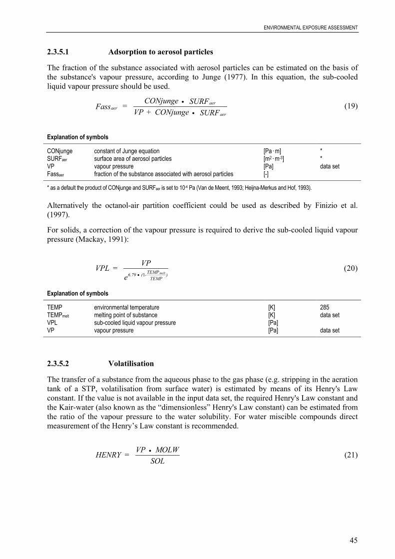
ENVIRONMENTAL EXPOSURE ASSESSMENT
45
2.3.5.1 Adsorption to aerosol particles
The fraction of the substance associated with aerosol particles can be estimated on the basis ofthe substance's vapour pressure, according to Junge (1977). In this equation, the sub-cooledliquid vapour pressure should be used.
aeraer
aerFass = CONjunge SURF
VP + CONjunge SURF•
•(19)
Explanation of symbols
CONjunge constant of Junge equation [Pa.m] *SURFaer surface area of aerosol particles [m2.m-3] *VP vapour pressure [Pa] data setFassaer fraction of the substance associated with aerosol particles [-]
* as a default the product of CONjunge and SURFaer is set to 10-4 Pa (Van de Meent, 1993; Heijna-Merkus and Hof, 1993).
Alternatively the octanol-air partition coefficient could be used as described by Finizio et al.(1997).
For solids, a correction of the vapour pressure is required to derive the sub-cooled liquid vapourpressure (Mackay, 1991):
VPL = VP
e6.79 ( -TEMPTEMP
)melt• 1(20)
Explanation of symbols
TEMP environmental temperature [K] 285TEMPmelt melting point of substance [K] data setVPL sub-cooled liquid vapour pressure [Pa]VP vapour pressure [Pa] data set
2.3.5.2 Volatilisation
The transfer of a substance from the aqueous phase to the gas phase (e.g. stripping in the aerationtank of a STP, volatilisation from surface water) is estimated by means of its Henry's Lawconstant. If the value is not available in the input data set, the required Henry's Law constant andthe Kair-water (also known as the “dimensionless” Henry's Law constant) can be estimated fromthe ratio of the vapour pressure to the water solubility. For water miscible compounds directmeasurement of the Henry’s Law constant is recommended.
HENRY = VP MOLWSOL• (21)
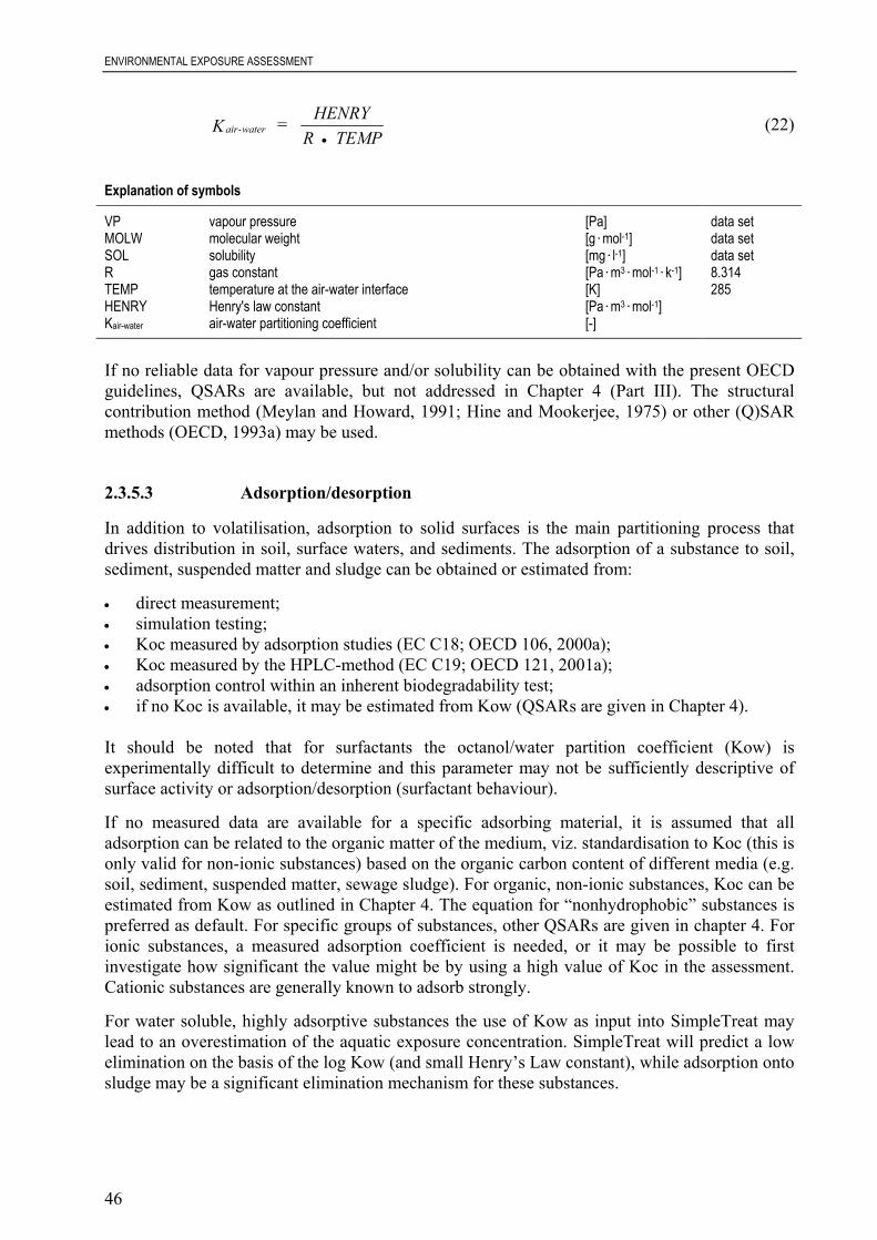
ENVIRONMENTAL EXPOSURE ASSESSMENT
46
air-waterK = HENRYR TEMP•
(22)
Explanation of symbols
VP vapour pressure [Pa] data setMOLW molecular weight [g.mol-1] data setSOL solubility [mg.l-1] data setR gas constant [Pa.m3.mol-1.k-1] 8.314TEMP temperature at the air-water interface [K] 285HENRY Henry's law constant [Pa.m3.mol-1]Kair-water air-water partitioning coefficient [-]
If no reliable data for vapour pressure and/or solubility can be obtained with the present OECDguidelines, QSARs are available, but not addressed in Chapter 4 (Part III). The structuralcontribution method (Meylan and Howard, 1991; Hine and Mookerjee, 1975) or other (Q)SARmethods (OECD, 1993a) may be used.
2.3.5.3 Adsorption/desorption
In addition to volatilisation, adsorption to solid surfaces is the main partitioning process thatdrives distribution in soil, surface waters, and sediments. The adsorption of a substance to soil,sediment, suspended matter and sludge can be obtained or estimated from:
• direct measurement;• simulation testing;• Koc measured by adsorption studies (EC C18; OECD 106, 2000a);• Koc measured by the HPLC-method (EC C19; OECD 121, 2001a);• adsorption control within an inherent biodegradability test;• if no Koc is available, it may be estimated from Kow (QSARs are given in Chapter 4).
It should be noted that for surfactants the octanol/water partition coefficient (Kow) isexperimentally difficult to determine and this parameter may not be sufficiently descriptive ofsurface activity or adsorption/desorption (surfactant behaviour).
If no measured data are available for a specific adsorbing material, it is assumed that alladsorption can be related to the organic matter of the medium, viz. standardisation to Koc (this isonly valid for non-ionic substances) based on the organic carbon content of different media (e.g.soil, sediment, suspended matter, sewage sludge). For organic, non-ionic substances, Koc can beestimated from Kow as outlined in Chapter 4. The equation for “nonhydrophobic” substances ispreferred as default. For specific groups of substances, other QSARs are given in chapter 4. Forionic substances, a measured adsorption coefficient is needed, or it may be possible to firstinvestigate how significant the value might be by using a high value of Koc in the assessment.Cationic substances are generally known to adsorb strongly.
For water soluble, highly adsorptive substances the use of Kow as input into SimpleTreat maylead to an overestimation of the aquatic exposure concentration. SimpleTreat will predict a lowelimination on the basis of the log Kow (and small Henry’s Law constant), while adsorption ontosludge may be a significant elimination mechanism for these substances.
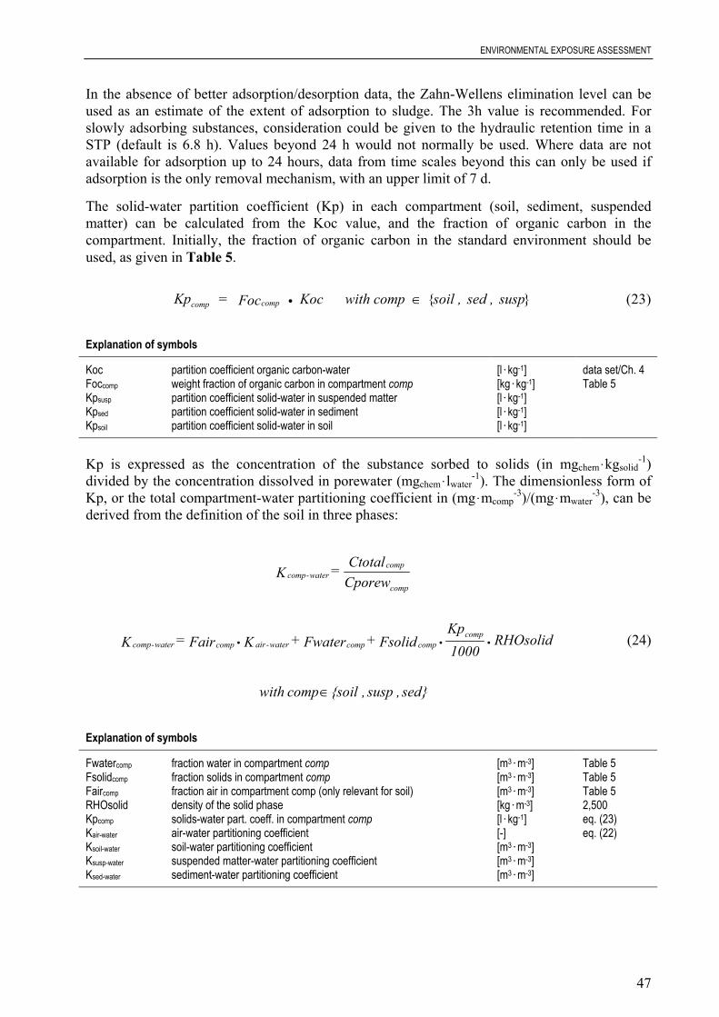
ENVIRONMENTAL EXPOSURE ASSESSMENT
47
In the absence of better adsorption/desorption data, the Zahn-Wellens elimination level can beused as an estimate of the extent of adsorption to sludge. The 3h value is recommended. Forslowly adsorbing substances, consideration could be given to the hydraulic retention time in aSTP (default is 6.8 h). Values beyond 24 h would not normally be used. Where data are notavailable for adsorption up to 24 hours, data from time scales beyond this can only be used ifadsorption is the only removal mechanism, with an upper limit of 7 d.
The solid-water partition coefficient (Kp) in each compartment (soil, sediment, suspendedmatter) can be calculated from the Koc value, and the fraction of organic carbon in thecompartment. Initially, the fraction of organic carbon in the standard environment should beused, as given in Table 5.
comp compKp = Foc Koc with comp soil , sed , susp• ∈ { } (23)
Explanation of symbols
Koc partition coefficient organic carbon-water [l.kg-1] data set/Ch. 4Foccomp weight fraction of organic carbon in compartment comp [kg.kg-1] Table 5Kpsusp partition coefficient solid-water in suspended matter [l.kg-1]Kpsed partition coefficient solid-water in sediment [l.kg-1]Kpsoil partition coefficient solid-water in soil [l.kg-1]
Kp is expressed as the concentration of the substance sorbed to solids (in mgchem.kgsolid-1)
divided by the concentration dissolved in porewater (mgchem.lwater-1). The dimensionless form of
Kp, or the total compartment-water partitioning coefficient in (mg.mcomp-3)/(mg.mwater
-3), can bederived from the definition of the soil in three phases:
sed} , susp ,{soil comp with
RHOsolid 1000Kp
Fsolid + Fwater + K Fair = K
CporewCtotal = K
compcompcompwater-aircompwater-comp
comp
compwater-comp
∈
••• (24)
Explanation of symbols
Fwatercomp fraction water in compartment comp [m3.m-3] Table 5Fsolidcomp fraction solids in compartment comp [m3.m-3] Table 5Faircomp fraction air in compartment comp (only relevant for soil) [m3.m-3] Table 5RHOsolid density of the solid phase [kg.m-3] 2,500Kpcomp solids-water part. coeff. in compartment comp [l.kg-1] eq. (23)Kair-water air-water partitioning coefficient [-] eq. (22)Ksoil-water soil-water partitioning coefficient [m3.m-3]Ksusp-water suspended matter-water partitioning coefficient [m3.m-3]Ksed-water sediment-water partitioning coefficient [m3.m-3]
ENVIRONMENTAL EXPOSURE ASSESSMENT
48
2.3.6 Abiotic and biotic degradation rates
In this section, the following processes are described:
• hydrolysis in surface water;• photolysis in surface water and in the atmosphere;• biodegradation in the sewage treatment plant;• biodegradation in the environmental compartments (surface water, soil, sediment).
Transport and transformation (“fate”) describe the distribution of a substance in the environment,or in organisms, and its changes with time (in concentration, chemical form, etc.), thus includingboth biotic and abiotic transformation processes. In general, the assessment of degradationprocesses should be based on data, which reflect the environmental conditions as realistically aspossible. Data from studies where degradation rates are measured under conditions that simulatethe conditions in various environmental compartments are preferred. The applicability of suchdata should, however, be judged in the light of any other degradation data including results fromscreening tests. Most emphasis is put on the simulation test results but in the absence of simulationtest data, degradation rates and half-lives have to be estimated from screening test data.
For substances where a range of degradation data is available, a “weight of evidence” approachshould be employed. When more than one simulation test result is available, a suitable half-lifein the higher end of the observed range should be selected taking into account the realism,relevance, quality and documentation of the studies in relation to environmental conditions.When more than one screening test result is available, positive test results should be consideredvalid, irrespective of negative results, when the scientific quality is good and the test conditionsare well documented, i.e. guideline criteria are fulfilled, including the use of non-adaptedinoculum (cf. OECD, 2001c). The results of screening tests may be negative due to toxic effectsof the test substance, whereas simulation tests employing a low concentration of the testsubstance may give a more realistic estimate of the degradation in the environment. By using allavailable degradability test data in this way, it is possible to establish a comprehensiveevaluation of the degradability of the substance.
In this section, methods for derivation of degradation rate constants are described for abioticdegradation (hydrolysis and photolysis) and biotic degradation (in soil, sediment, water, andsewage treatment). For hydrolysis and photolysis, only primary degradation is measured. Ingeneral, risk assessment focuses on the parent compound. Nevertheless, if stable degradationproducts are formed, the risk assessment should include these. It is possible that the rate ofreaction is such that only the products need to be considered, or in intermediate cases both thesubstance and the degradation products will require consideration. It is important to haveinformation about which chemical species were responsible for any effects that were observed inthe aquatic toxicity studies.
Where substances degrade by complex interaction mechanisms, for example abiotic degradationfollowed by biodegradation, and where there are no internationally recognised protocols forsimulation tests, the use of relevant field data could be considered provided that the kinetics offull mineralisation or formation of possible metabolites have been determined.
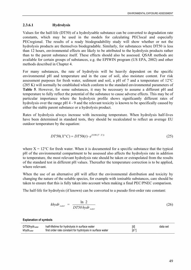
ENVIRONMENTAL EXPOSURE ASSESSMENT
49
2.3.6.1 Hydrolysis
Values for the half-life (DT50) of a hydrolysable substance can be converted to degradation rateconstants, which may be used in the models for calculating PEClocal and especiallyPECregional. The results of a ready biodegradability study will show whether or not thehydrolysis products are themselves biodegradable. Similarly, for substances where DT50 is lessthan 12 hours, environmental effects are likely to be attributed to the hydrolysis products ratherthan to the parent substance itself. These effects should also be assessed. QSAR methods areavailable for certain groups of substances, e.g. the EPIWIN program (US EPA, 2002) and othermethods described in Chapter 4.
For many substances, the rate of hydrolysis will be heavily dependent on the specificenvironmental pH and temperature and in the case of soil, also moisture content. For riskassessment purposes for fresh water, sediment and soil, a pH of 7 and a temperature of 12°C(285 K) will normally be established which conform to the standard environmental parameters ofTable 5. However, for some substances, it may be necessary to assume a different pH andtemperature to fully reflect the potential of the substance to cause adverse effects. This may be ofparticular importance where the hydrolysis profile shows significantly different rates ofhydrolysis over the range pH 4 - 9 and the relevant toxicity is known to be specifically caused byeither the stable parent substance or a hydrolysis product.
Rates of hydrolysis always increase with increasing temperature. When hydrolysis half-liveshave been determined in standard tests, they should be recalculated to reflect an average EUoutdoor temperature by the equation:
))(08.0()(50)(50 XTetDTCXDT −⋅⋅=° (25)
where X = 12°C for fresh water. When it is documented for a specific substance that the typicalpH of the environmental compartment to be assessed also affects the hydrolysis rate in additionto temperature, the most relevant hydrolysis rate should be taken or extrapolated from the resultsof the standard test in different pH values. Thereafter the temperature correction is to be applied,where relevant.
When the use of an alternative pH will affect the environmental distribution and toxicity bychanging the nature of the soluble species, for example with ionisable substances, care should betaken to ensure that this is fully taken into account when making a final PEC/PNEC comparison.
The half-life for hydrolysis (if known) can be converted to a pseudo first-order rate constant:
waterwater
khydr = DT50 hydr
ln 2 (26)
Explanation of symbols
DT50hydrwater half-lifetime for hydrolysis in surface water [d] data setkhydrwater first order rate constant for hydrolysis in surface water [d-1]

ENVIRONMENTAL EXPOSURE ASSESSMENT
50
2.3.6.2 Photolysis in water
In the vast majority of surface water bodies dissolved organic matter is responsible for intensivelight attenuation. Thus photolysis processes are normally restricted to the upper zones of waterbodies. Indirect processes like photo-sensitisation or reaction with oxygen transients (1O2, OH-radicals, ROO-radicals) may significantly contribute to the overall breakdown rate.Photochemical degradation processes in water may only become an important fate process forsubstances, which are persistent to other degradation processes (e.g. biodegradation andhydrolysis). The experimental determination of the quantum yield (OECD, 1992c) and the UV-absorption spectrum of the substance are prerequisites for estimating the rate ofphotodegradation in surface water. Due to high seasonal variation in light flux, photochemicaldegradation should only be based on average EU conditions. Methods to derive averagedegradation rates which can be used in the model calculation of PECregional are described inZepp and Cline (1977) and Frank and Klöppfer (1989).
The following aspects have to be considered when estimating the photochemical transformationin natural water bodies:
• the intensity of the incident light depends on seasonal and geographic conditions and varieswithin wide ranges. For long-term considerations average values can be used while forshort-term exposure an unfavourable solar irradiance (winter season) should be chosen;
• in most natural water bodies, the rate of photoreaction is affected by dissolved andsuspended matter. Since the concentration of the substance under consideration is normallylow compared to the concentration of e.g. dissolved humic acids, the natural constituentsabsorb by far the larger portion of the sunlight penetrating the water bodies.
Using the standard parameters of the regional model (i.e. a water depth of 3 m and aconcentration of suspended matter of 15 mg/l), the reduction in light intensity is higher than 98%through the water column.
Indirect (sensitised) photochemical reactions should only be included in the overall breakdownrate of water bodies if there is clear evidence that this pathway is not of minor importancecompared to other processes and its effectiveness can be quantified. For facilitating the complexcalculation of phototransformation processes in natural waters computer programmes have beendeveloped (e.g. ABIWAS by Frank and Klöppfer, 1989; GC-SOLAR by Zepp and Cline, 1977).
In practice it will not be possible to easily demonstrate that photodegradation in water issignificant in the environment.
A value for the half-life for photolysis in water (if known) can be converted to a pseudo first-order rate constant:
waterwater
kphoto = DT50 photo
ln 2 (27)
Explanation of symbols
DT50photowater half-lifetime for photolysis in surface water [d] data setkphotowater first order rate constant for photolysis in surface water [d-1]

ENVIRONMENTAL EXPOSURE ASSESSMENT
51
2.3.6.3 Photochemical reactions in the atmosphere
Although for some substances direct photolysis may be an important breakdown process, themost effective elimination process in the troposphere for most substances results from reactionswith photochemically generated species like OH radicals, ozone and nitrate radicals. Thespecific first order degradation rate constant of a substance with OH-radicals (kOH incm3.molecule-1.s-1) can either be determined experimentally (OECD, 1992c) or estimated by(Q)SAR-methods and other methods described in Chapter 4 (US EPA, 2002). By relating kOH tothe average OH-radical concentration in the atmosphere, the pseudo-first order rate constant inair is determined:
kdegair = kOH • OHCONCair • 24 • 3600 (28)
Explanation of symbols
kOH specific degradation rate constant with OH-radicals [cm3.molec-1.s-1] data set/Ch.4OHCONCair concentration of OH-radicals in atmosphere [molec.cm-3] 5.105 *kdegair pseudo first order rate constant for degradation in air [d-1]
*The global annual average OH-radical concentration can be assumed to be 5.105 molecules.cm-3 (BUA, 1992).
Degradation in the atmosphere is an important process and it is essential to consider whether itcan affect the outcome, particularly for high tonnage substances when the regional concentrationmay be significant. Photodegradation data in the atmosphere must be evaluated with somecare. Highly persistent substances may be reported as rapidly degraded in air underenvironmental conditions where the chemical could be in large amounts in the gas phase. Inthe real environment, most of the substance may be associated to particles or aerosol and thereal atmospheric half-life could be orders of magnitude higher.
2.3.6.4 Biodegradation in a sewage treatment plant
The assessment of biodegradability and/or removal in sewage treatment plants should preferablybe based on results from tests simulating the conditions in treatment plants. Such a test may bethe OECD 303 test (2001b) or equivalent. For further guidance on use of STP simulation testresults, see Section 2.3.7.
The ready biodegradability tests that are used at the moment are aimed at measuring the ultimatebiodegradability of a substance. They do not give a quantitative estimate of the removalpercentage in a wastewater treatment plant. Therefore, in order to make use of thebiodegradation test results that are available and requested in the present chemical legislation, itis necessary to assign rate constants to the results of the standard tests for use in STP-models.These constants are based on a relatively limited number of empirical data. However, sincedirect measurements of degradation rates at environmentally relevant concentrations are oftennot available, a pragmatic solution to this problem has been found. For the purpose of modellinga sewage treatment plant (STP), the rate constants of Table 6 were derived from thebiodegradation screening tests. All constants in Table 6 have the following prerequisites:

ENVIRONMENTAL EXPOSURE ASSESSMENT
52
• they are only used for the water-dissolved fraction of the substance. Partitioning betweenwater and sludge phases should be calculated prior to the application of the rate constant;
• sufficiently valid data from internationally standardised tests are preferred;
Data from non-standardised tests and/or tests not performed according to the principles of GLPmay be used if expert judgement has confirmed them to be equivalent to results from thestandardised degradation tests on which the calculation models, e.g. SimpleTreat, are based. Thesame applies to STP-measured data, i.e., in-situ influent/effluent measurements.
Table 6 Elimination in sewage treatment plants: Extrapolation from test results to rate constants in STP model (SimpleTreat)
Test result Rate constant k.(h-1)
Readily biodegradable a) 1
Readily, but failing 10-d window a) 0.3
Inherently biodegradable, fulfilling specific criteria b) 0.1
Inherently biodegradable, not fulfilling specific criteria b) 0
Not biodegradable 0
Notes to Table 6:a) Ready biodegradability testing (28 d) (92/69/ EU Annex V C.4 A-F, or respectively, OECD 301A-F (1992f) or equivalent according to
expert judgement).Ready biodegradability tests are screening tests for identifying substances that, based on general experience, are assumed to undergorapid and ultimate biodegradation in the aerobic environment. However, a negative result does not necessarily mean that thesubstance will not be biodegraded in, e.g., a sewage treatment plant.The degree of ultimate degradation may be followed by determination of the loss of dissolved organic carbon (DOC), the evolution ofcarbon dioxide or the amount of oxygen consumed. It is generally accepted that a substance is considered to be readily biodegradableif the substance fulfils the pass criteria of a test for ready biodegradability (cf. the Annex V methods or the OECD guidelines) which mayinclude the concept of the 10 days time window as a simple kinetic criterion. All percentage biodegradation results refer to truebiodegradation i.e. mineralisation excluding abiotic elimination processes (e.g. volatilisation, adsorption). This means thatcorresponding data in adequate control vessels must be generated during biodegradation testing. The test may be continued beyond28 days if biodegradation has started but does not reach the required pass criteria for final mineralisation: in this case however, thesubstance would not be regarded as being readily biodegradable. If the substance reaches the biodegradation pass levels within 28days but not within the 10-day time window, a biodegradation rate constant of 0.3 h-1 is assumed. In case that only old readybiodegradation test results (i.e. tests executed prior to the introduction of the 10 days time window criterion and documenting only onthe pass level) are available a rate constant of 0.3 h-1 should be applied in case the pass level is reached. Based on weight of evidence(e.g. several old test results) a rate constant of 1 h-1 may be justified by expert judgement.If the substance is found to be not readily biodegradable, it is necessary to check whether it was inhibitory to microbial activity at theconcentration used in the biodegradability test. If the substance is inhibitory, it may be re-tested at low, non-inhibitory concentrations ina test simulating the conditions in a sewage treatment plant (e.g. OECD guideline 303, 2001b; ISO 11733 or equivalent). If appropriate,re-testing in another more suitable ready biodegradability test (e.g. Closed Bottle test) may be considered. Re-testing in a modifiedready biodegradability test at a much lower concentration (i.e. more than 10 times lower than prescribed) cannot generally berecommended because suitable simulation test methods are available.
b) Inherent biodegradability testing (28d) (87/302/EEC, respectively, OECD 302B-C (1981d-1992g) or equivalent according to expertjudgement).Inherent biodegradability tests are designed to assess whether the substance has any potential for biodegradation. A negative resultwill normally mean that non-biodegradability (persistence) should be assumed. A positive result, on the other hand, indicates that thesubstance will not persist indefinitely in the environment. In those cases where a more accurate prediction of degradation kinetics intreatment plants is required, sewage treatment plant simulation tests (e.g. OECD guideline 303, 2001b; ISO 11733 or equivalent)should be conducted.In tests for inherent biodegradability, the test conditions are designed to be more favourable to the microorganisms in that the ratio ofsubstance to cells is lower than in the ready tests and there is no requirement for the (bio)degradation to follow a time pattern as in theready tests. Also, pre-exposure of the inoculum resulting in pre-adaptation of the microorganisms may be allowed. The time permittedfor the study is limited to 28 days, but it may be continued for much longer; 6 months has been suggested as the maximum duration forthe test. The results obtained in a test of more than 28 days are not comparable with those obtained in less than this period.Usually, more than 70% (bio)degradation within 28 days indicates that the substance is inherently biodegradable. However,extrapolation of the results of the inherent tests should be done with great caution because of the strongly favourable conditions forbiodegradation that are present in these tests. Therefore, a substance that passes an inherent test should in principle be given a rate
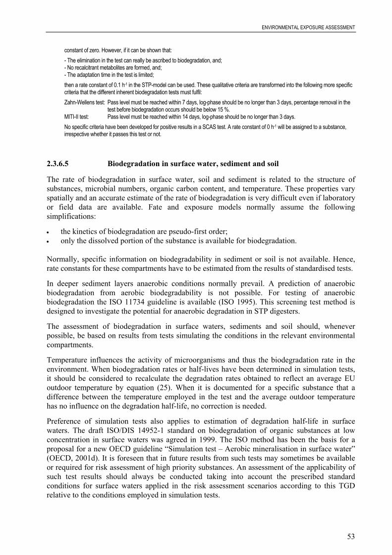
ENVIRONMENTAL EXPOSURE ASSESSMENT
53
constant of zero. However, if it can be shown that:- The elimination in the test can really be ascribed to biodegradation, and;- No recalcitrant metabolites are formed, and;- The adaptation time in the test is limited;then a rate constant of 0.1 h-1 in the STP-model can be used. These qualitative criteria are transformed into the following more specificcriteria that the different inherent biodegradation tests must fulfil:Zahn-Wellens test: Pass level must be reached within 7 days, log-phase should be no longer than 3 days, percentage removal in the
test before biodegradation occurs should be below 15 %.MITI-II test: Pass level must be reached within 14 days, log-phase should be no longer than 3 days.No specific criteria have been developed for positive results in a SCAS test. A rate constant of 0 h-1 will be assigned to a substance,irrespective whether it passes this test or not.
2.3.6.5 Biodegradation in surface water, sediment and soil
The rate of biodegradation in surface water, soil and sediment is related to the structure ofsubstances, microbial numbers, organic carbon content, and temperature. These properties varyspatially and an accurate estimate of the rate of biodegradation is very difficult even if laboratoryor field data are available. Fate and exposure models normally assume the followingsimplifications:
• the kinetics of biodegradation are pseudo-first order;• only the dissolved portion of the substance is available for biodegradation.
Normally, specific information on biodegradability in sediment or soil is not available. Hence,rate constants for these compartments have to be estimated from the results of standardised tests.
In deeper sediment layers anaerobic conditions normally prevail. A prediction of anaerobicbiodegradation from aerobic biodegradability is not possible. For testing of anaerobicbiodegradation the ISO 11734 guideline is available (ISO 1995). This screening test method isdesigned to investigate the potential for anaerobic degradation in STP digesters.
The assessment of biodegradation in surface waters, sediments and soil should, wheneverpossible, be based on results from tests simulating the conditions in the relevant environmentalcompartments.
Temperature influences the activity of microorganisms and thus the biodegradation rate in theenvironment. When biodegradation rates or half-lives have been determined in simulation tests,it should be considered to recalculate the degradation rates obtained to reflect an average EUoutdoor temperature by equation (25). When it is documented for a specific substance that adifference between the temperature employed in the test and the average outdoor temperaturehas no influence on the degradation half-life, no correction is needed.
Preference of simulation tests also applies to estimation of degradation half-life in surfacewaters. The draft ISO/DIS 14952-1 standard on biodegradation of organic substances at lowconcentration in surface waters was agreed in 1999. The ISO method has been the basis for aproposal for a new OECD guideline “Simulation test – Aerobic mineralisation in surface water”(OECD, 2001d). It is foreseen that in future results from such tests may sometimes be availableor required for risk assessment of high priority substances. An assessment of the applicability ofsuch test results should always be conducted taking into account the prescribed standardconditions for surface waters applied in the risk assessment scenarios according to this TGDrelative to the conditions employed in simulation tests.

ENVIRONMENTAL EXPOSURE ASSESSMENT
54
When results from biodegradation tests simulating the conditions in surface waters are notavailable, the use of results from various screening tests may be considered. Table 7 gives aproposal for first order rate constants for surface water to be used in local and especially,regional models, based on the results of screening tests for biodegradability. The proposal isbased on general experience in relation to available data on biodegradation half-lives in surfacewaters of readily and not readily biodegradable substances.
The assigned degradation half-lives of an inherently biodegradable substance of 150 days insurface water (Table 7) and 300 – 30,000 days in soil and sediment (Table 8) will only affectthe predicted regional concentration provided that the residence time of the substance is muchlarger than the assigned half-life (i.e. only for substances present in soil compartment andsediment).
It is noted that the conditions in laboratory screening tests are very different from the conditionsin various environmental compartments. The concentration of the test substance is several ordersof magnitude greater in these screening tests than the concentrations of xenobiotic substancesgenerally occurring in the environment and thus the kinetic regimes are significantly different.The temperature is also higher in screening tests than those generally occurring in theenvironment. Furthermore the microbial biomass is normally lower under environmentalconditions than those occurring in these screening tests, especially in the tests for inherentbiodegradability. These factors are taken into account in the proposed degradation rates and half-lives in Tables 7 and 8.
Table 7 First order rate constants and half-lives for biodegradation in surface water based on results of screening tests onbiodegradability a)
Test result Rate constant k (d-1) Half-life (d)
Readily biodegradable 4.7.10-2 15
Readily, but failing 10-d window b) 1.4.10-2 50
Inherently biodegradable c) 4.7.10-3 150
Not biodegradable 0 ∞
Notes to Table 7:a) For use in exposure models these half-lives do not need to be corrected for different environmental temperatures.b) The 10-day time window concept does not apply to the MITI test. The value obtained in a 14-d window is regarded as acceptable in the
Closed Bottle method, if the number of bottles that would have been required to evaluate the 10-d window would cause the test tobecome too unwieldy.
c) Only those inherently degradable substances that fulfil the criteria described in note b) to Table 6 above. The half-life of 150 daysreflects a present "best expert judgement".
The general experience is that a substance passing a test for ready biodegradability may undermost environmental conditions be rapidly degraded and the estimated half-lives for suchsubstances (cf. Table 7) should therefore be regarded as being in accordance with “the realisticworst-case concept”. An OECD guidance document for classification of chemicals hazardous forthe aquatic environment (OECD, 2001c) contains a chapter on interpretation of degradation data.Even though this guidance relates to hazard classification and not risk assessment, many of theconsiderations and interpretation principles may also apply in a risk assessment context. Onedifference is of course that in the risk assessment context not only a categorisation of thesubstance (i.e. a classification) is attempted, but instead an approximate half-life is estimated.
ENVIRONMENTAL EXPOSURE ASSESSMENT
55
Another difference is that for risk assessment, the availability of high quality test data is requiredin virtually all cases and further testing may therefore be required in the case of low quality data.
In distribution models, calculations are performed for compartments each consisting ofhomogeneous sub-compartments, i.e. surface water containing dissolved organic carbon andsuspended matter, sediment containing porewater and a solid phase, and soil containing air,porewater and a solid phase. Since it is assumed that no degradation takes place in the sorbedphase, the rate constant for the surface water, bulk sediment or soil in principle depends on thesuspended matter/water, sediment/water or soil/water partition coefficient of the substance. Withincreasing hydrophobicity (sorption) of the substance, the freely dissolved fraction present in thewater phase available for degradation decreases, and therefore the overall rate constant shouldalso decrease. However, for surface waters the influence of sorption is already comprised in thedegradation rates when they are determined for bulk water in simulation tests employing thesame conditions as in the aquatic environment. Neither is it needed to consider the influence ofsorption processes when rate constants are established from screening test results due to thewell-established practice to conclude on biodegradability in the environment from such data.
Also for assessment of biodegradation in soil or sediment, data from relevant simulation tests arepreferred. Simulation tests such as the OECD 307 “Aerobic and anaerobic transformation insoil” (OECD, 2000b; EU Annex V draft C.23) and the OECD 308 “Aerobic and anaerobictransformation in aquatic sediment systems” (OECD, 2000c; EU Annex V draft C.24) areavailable. The basis for these methods was initially developed for pesticides, e.g. guidelines ofBBA (BBA, 1986; BBA, 1990a) and US EPA. The draft ISO/DIS 14592-1 standard includes anoption for determination of biodegradability in a surface water/sediment suspension. Of coursethis test does not directly simulate the conditions in non-disturbed sediment. The measured half-life in water/sediment tests may be dependent on the relative volume of water and sedimentemployed in the test.
When such simulation test data are available, the applicability of the results from the tests shouldbe evaluated on a case-by-case basis employing expert judgement when used in a riskassessment.
When no data from tests simulating the conditions in soil or sediment are available, the use ofscreening test data may be considered. The guidance for use of such data is based on the generalrecognition that for substances with low Kp values at present not enough empirical data areavailable to assume some sort of dependence of the soil biodegradation half-life on thesolids/water partition coefficient. Nevertheless, for substances with high Kp values there isevidence that some sort of Kp dependence exists. Therefore degradation half-life classes for(bulk) soil, partly based on Kp are presented in Table 8. If a half-life from a surface watersimulation test is available it may, in a similar manner, form the basis for the establishment of ahalf-life in soil. The half-lives indicated in the table are considered conservative.
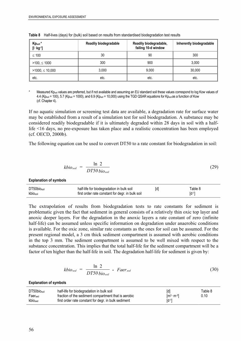
ENVIRONMENTAL EXPOSURE ASSESSMENT
56
Table 8 Half-lives (days) for (bulk) soil based on results from standardised biodegradation test results
Kpsoil *[l.kg-1]
Readily biodegradable Readily biodegradable,failing 10-d window
Inherently biodegradable
≤ 100 30 90 300
>100, ≤ 1000 300 900 3,000
>1000, ≤ 10,000 3,000 9,000 30,000
etc. etc. etc. etc.
* Measured Kpsoil values are preferred, but if not available and assuming an EU standard soil these values correspond to log Kow values of4.4 (Kpsoil = 100), 5.7 (Kpsoil = 1000), and 6.9 (Kpsoil = 10,000) using the TGD QSAR equations for Kpsoil as a function of Kow(cf. Chapter 4).
If no aquatic simulation or screening test data are available, a degradation rate for surface watermay be established from a result of a simulation test for soil biodegradation. A substance may beconsidered readily biodegradable if it is ultimately degraded within 28 days in soil with a half-life <16 days, no pre-exposure has taken place and a realistic concentration has been employed(cf. OECD, 2000b).
The following equation can be used to convert DT50 to a rate constant for biodegradation in soil:
soilsoil
kbio = DT50 bio
ln 2 (29)
Explanation of symbols
DT50biosoil half-life for biodegradation in bulk soil [d] Table 8kbiosoil first order rate constant for degr. in bulk soil [d-1]
The extrapolation of results from biodegradation tests to rate constants for sediment isproblematic given the fact that sediment in general consists of a relatively thin oxic top layer andanoxic deeper layers. For the degradation in the anoxic layers a rate constant of zero (infinitehalf-life) can be assumed unless specific information on degradation under anaerobic conditionsis available. For the oxic zone, similar rate constants as the ones for soil can be assumed. For thepresent regional model, a 3 cm thick sediment compartment is assumed with aerobic conditionsin the top 3 mm. The sediment compartment is assumed to be well mixed with respect to thesubstance concentration. This implies that the total half-life for the sediment compartment will be afactor of ten higher than the half-life in soil. The degradation half-life for sediment is given by:
sedsoil
sedkbio = DT50 bio
Faerln 2
• (30)
Explanation of symbols
DT50biosoil half-life for biodegradation in bulk soil [d] Table 8Faersed fraction of the sediment compartment that is aerobic [m3.m-3] 0.10kbiosed first order rate constant for degr. in bulk sediment [d-1]
ENVIRONMENTAL EXPOSURE ASSESSMENT
57
The remarks in the section on soil biodegradation regarding use of half-lives derived in surfacewater simulation tests may also apply for sediments.
2.3.6.6 Overall rate constant for degradation in surface water
In surface water, the substance may be transformed through photolysis, hydrolysis, andbiodegradation. For calculation of the PECregional, the rate constants for these processes can besummed into one, overall degradation rate constant. It should be noted that different types ofdegradation (primary and ultimate) are added. This is done for modelling purposes only. Itshould also be noted that measurements on one degradation process might in fact already includethe effects of other processes. For example, hydrolysis can occur under the conditions of abiodegradation test or a test of photodegradation, and so may already be comprised by themeasured rate from these tests. In order to add the rates of different processes, it should bedetermined that the processes occur in parallel and that their effects are not already included inthe rates for other processes. If exclusion of hydrolysis from the other degradation rates cannotbe confirmed its rate constant should be set to zero. The equation below relates to primarydegradation. If the primary degradation is not the rate-limiting step in the total degradationsequence and degradation products accumulate, then also the degradation product(s) formed inthe particular process (e.g. hydrolysis) should be assessed. If this cannot be done or is notpractical, the rate constant for the process should be set to zero.
kdegwater = khydrwater + kphotowater + kbiowater (31)
Explanation of symbols
khydrwater first order rate constant for hydrolysis in surface water [d-1] eq. (26)kphotowater first order rate constant for photolysis in surface water [d-1] eq. (27)kbiowater first order rate constant for biodegradation in surface water [d-1] Table 7kdegwater total first order rate constant for degradation in surface water [d-1]
2.3.7 Elimination processes prior to the release to the environment
2.3.7.1 Wastewater treatment
In this section, the following parameters are derived:
• emission from a sewage treatmentplant to air;• concentration in sewage sludge;• concentration in effluent of a sewage treatment plant;• PEC for microorganisms in a sewage treatment plant.
Elimination refers to the reduction in the concentration of substances in gaseous or aqueousdischarges prior to their release to the environment. Elimination from the water phase may occurby physical as well as chemical or biochemical processes. In a sewage treatment plant (STP),one of the main physical processes is settling of suspended matter which will also removeadsorbed material. Physical processes do not degrade a substance but transfer it from one phaseto another e.g. from liquid to solid. In the case of volatile substances, the aeration process will
ENVIRONMENTAL EXPOSURE ASSESSMENT
58
enhance their removal from the water phase by “stripping” them from the solid/liquid phases tothe atmosphere. Substances may be removed from exhaust gaseous streams by scrubbing e.g. byadsorption on a suitable material or by passing through a trapping solution.
Wastewater treatment
One of the critical questions to answer in determining the PEC for the aquatic environment iswhether or not the substance will pass through a wastewater treatment plant and if yes, throughwhich kind of treatment plant before being discharged into the environment. The situation in theMember States concerning percentage connection to sewage works is quite diverse (seeAppendix XII). The percentage connection rate across the Community is subject to improvementdue to the implementation of the Urban Waste Water Treatment Directive (UWWTD,91/271/EEC). This directive requires Member States (via transposition into national legislation)to ensure that wastewater from all agglomerations of > 2,000 population equivalents is collectedand treated minimally by secondary treatment. The time limit for implementation of the directiveis 31/12/98, 31/12/2000 or 31/12/2005 dependent on the size of the agglomeration and thesensitivity of the receiving water body. An interim figure of 80% connection to wastewatertreatment is proposed for the regional standard environment. This value is thought to berepresentative for the actual situation in large urban areas at the time of revision of the TGD.Article 6 of the UWWTD allows Member States to declare non sensitive areas for whichdischarged wastewater from agglomerations between 10,000 and 150,000 populationequivalents, which are located at the sea and from agglomerations between 2,000 and 10,000population equivalents located at estuaries does not have to be treated biologically but onlymechanically (primary treatment). It is notable that 4 Member States have applied this article,corresponding to < 9% of the organic load (in terms of population equivalents).
The situation with respect to wastewater treatment at industrial installations is less clear. It maybe assumed that many of the larger industrial installations are either connected to a municipalwastewater treatment plant or have treatment facilities on site. In many cases, these treatmentplants are not biological treatment plants but often physico-chemical treatment plants in whichorganic matter is flocculated by auxiliary agents e.g. by iron salts followed by a sedimentationprocess resulting in a reduction of organic matter measured as COD of about 25-50%.
In the present document, the above-described situation is taken into account as follows:
• on a local scale, it is assumed that wastewater will pass through a STP before beingdischarged into the environment. Nevertheless, for the largest PEClocal in surface water, itis necessary to determine an aquatic PEClocal assuming that no sewage treatment will takeplace. This value should be determined in addition to the normal PEC that assumes sewagetreatment to flag for possible local problems (this PEC/PNEC ratio will not normally beused in risk characterisation). The alternative/additional PEC can be used to explore thepossibility of environmental impact in regions or industrial sectors where percentageconnection to sewage works is currently low, so as to give indications to local authorities forneeds of possible local risk reductions. The PEC without considering a STP-treatment willnot be used in the exposure assessment, unless the substance considered has a specific usecategory where direct discharge to water is widely practised;
• for a standard regional scale environment (definition see Section 2.3.8.1) it is assumed that80% of the wastewater is treated in a biological STP and the remaining 20% releaseddirectly into surface waters (although mechanical treatment has some effect on eliminatingorganic matter, this is neglected because on the other hand stormwater overflows usuallyresult in direct discharges to surface water even in the case of biological treatment. It is

ENVIRONMENTAL EXPOSURE ASSESSMENT
59
assumed that these two adverse effects compensate each other more or less with regard tothe pollution of the environment).
The degree of removal in a wastewater treatment plant is determined by the physico-chemicaland biological properties of the substance (biodegradation, adsorption onto sludge,sedimentation of insoluble material, volatilisation) and the operating conditions of the plant. Asthe type and amount of data available on degree of removal may vary, the following order ofpreference should be considered:
Measured data in full scale STP
The percentage removal should preferably be based upon measured influent and effluentconcentrations. As with measured data from the environment, the measured data from STPsshould be assessed with respect to their adequacy and representativeness.
Consideration must be given to the fact that the effectiveness of elimination in treatment plants isquite variable and depends on operational conditions, such as retention time in the aeration tank,aeration intensity, influent concentration, age and adaptation of sludge, extent of utilisation,rainwater retention capacity, etc. The data may be used provided that certain minimum criteriahave been met, e.g. the measurements have been carried out over a longer period of time.Furthermore, consideration should be given to the fact that removal may be due to stripping oradsorption (not degradation). In case no mass balance study has been performed, the percentageof transport to air or sludge should be estimated, e.g. by scaling the fractions to air and sludgefrom the tables in Appendix II to the measured removal.
Data from dedicated STPs should be used with caution. For example, when measured data areavailable for highly adapted STPs on sites producing high volume site-limited intermediates,these data should only be used for the assessment of this specific use category of the substance.
Simulation test data
Simulation testing is the examination of the potential of a substance to biodegrade in a laboratorysystem designated to represent either the activated sludge-based aerobic treatment stage of awastewater treatment plant or other environmental situations, for example a river. Thewastewater treatment process can be studied in the laboratory by, e.g., the updated OECDguideline on simulation testing of aerobic sewage treatment (OECD, 2001b) or the olderCoupled Units Test (OECD, 1981b). Removability is determined by monitoring the changes inDOC (Dissolved Organic Carbon) and/or COD (Chemical Oxygen Demand). A number ofguidelines have recently been prepared, e.g. ISO/DIS 14952-1, draft OECD (2001d), OECD 307(soil, 2000b), draft EU Annex V C.23, OECD 308 (sediment, 2000c), draft EU Annex V C.24.
The Coupled Units Test is not suitable for adsorptive, poorly water-soluble and volatilesubstances because it is an open test and is only based on DOC analysis. Since, in addition, it ispossible that adsorptive or volatile metabolites may be formed during biological degradation,this test cannot differentiate between biological degradation and other elimination processes.Investigations with a closed vessel version of the Coupled Units Test using radioactivelylabelled substances have been performed which would allow a determination of the completemass balance and would also be suitable for volatile or adsorptive substances. However, there isno international standard method available for this modified test.
There is insufficient information available on the applicability of elimination data from thelaboratory test to the processes of a real sewage plant. The results can be extrapolated to

ENVIRONMENTAL EXPOSURE ASSESSMENT
60
degradation in the real environment only if the concentrations that were used in the test are in thesame order of magnitude as the concentrations that are to be expected in the real environment. Ifthis is not the case, extrapolation can seriously overestimate the degradation rates especiallywhen the extrapolation goes from high to low concentrations. If concentrations are in the sameorder of magnitude then the results of these tests can be used quantitatively to estimate thedegree of removal of substances in a mechanical-biological STP.
If a complete mass balance is determined, the fraction removed by adsorption and strippingshould be used for the calculation of sludge and air concentrations. In case no mass balancestudy has been performed, the percentage of transport to air or sludge should be estimated forexample by using the tables in Appendix II.
Modelling STP
If there are no measured data available, the degree of removal can be estimated by means of awastewater treatment plant model using log Kow (Koc or more specific partition coefficients canalso be used; see Section 2.3.5), Henry's Law constant and the results of biodegradation tests asinput parameters. However, it should be remembered that the distribution behaviour oftransformation products is not considered by this approach. It is proposed to use in the screeningphase of exposure assessment a revised version of the sewage treatment plant model SimpleTreat(Struijs et al., 1991). This model is a multi-compartment box model, calculating steady-stateconcentrations in a sewage treatment plant, consisting of a primary settler, an aeration tank and aliquid-solid separator. With SimpleTreat, the sewage treatment plant is modelled for an averagesize treatment plant based on aerobic degradation by active sludge, and consisting of 9compartments (see Figure 6). Depending on the test results for ready and/or inherentbiodegradability of a substance, specific first order biodegradation rate constants are assigned tothe compound. An improved process formulation for volatilisation from the aeration tank, whichis also applicable to semi-volatile substances (Mikkelsen, 1995), has been incorporated in therevised version.
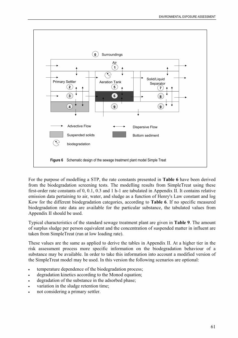
ENVIRONMENTAL EXPOSURE ASSESSMENT
61
For the purpose of modelling a STP, the rate constants presented in Table 6 have been derivedfrom the biodegradation screening tests. The modelling results from SimpleTreat using thesefirst-order rate constants of 0, 0.1, 0.3 and 1 h-1 are tabulated in Appendix II. It contains relativeemission data pertaining to air, water, and sludge as a function of Henry's Law constant and logKow for the different biodegradation categories, according to Table 6. If no specific measuredbiodegradation rate data are available for the particular substance, the tabulated values fromAppendix II should be used.
Typical characteristics of the standard sewage treatment plant are given in Table 9. The amountof surplus sludge per person equivalent and the concentration of suspended matter in influent aretaken from SimpleTreat (run at low loading rate).
These values are the same as applied to derive the tables in Appendix II. At a higher tier in therisk assessment process more specific information on the biodegradation behaviour of asubstance may be available. In order to take this information into account a modified version ofthe SimpleTreat model may be used. In this version the following scenarios are optional:
• temperature dependence of the biodegradation process;• degradation kinetics according to the Monod equation;• degradation of the substance in the adsorbed phase;• variation in the sludge retention time;• not considering a primary settler.
Primary Settler Aeration TankSolid/Liquid
Separator2
3
5
6
7
8
1Air
Surroundings0
Advective Flow Dispersive Flow
Suspended solids Bottom sediment
biodegradation
4 9 9
Figure 6 Schematic design of the sewage treatment plant model Simple Treat
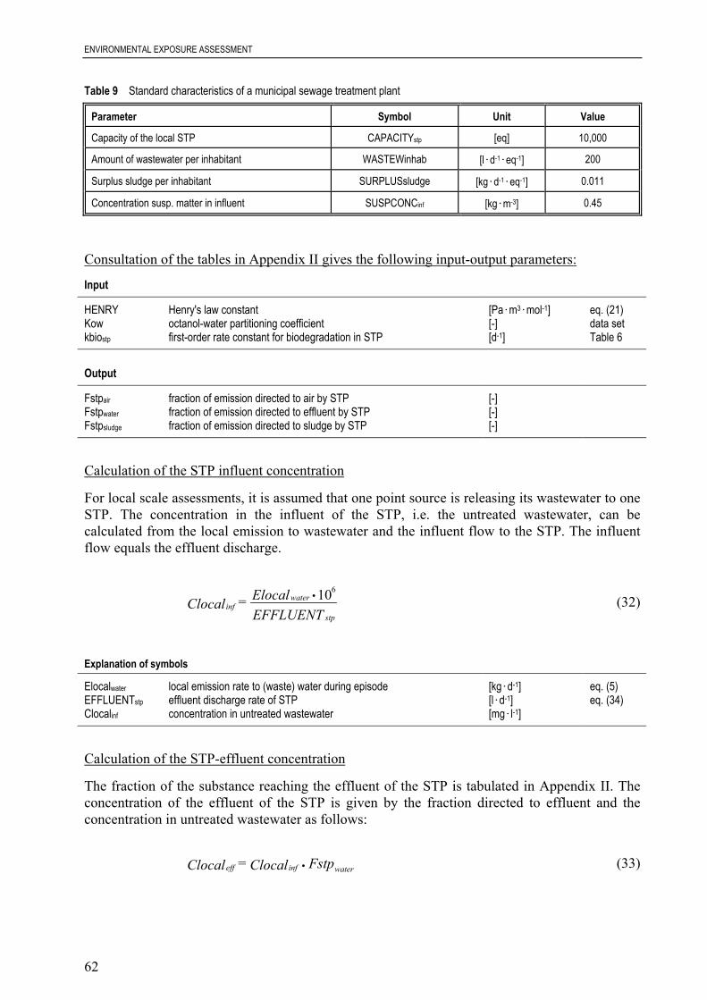
ENVIRONMENTAL EXPOSURE ASSESSMENT
62
Table 9 Standard characteristics of a municipal sewage treatment plant
Parameter Symbol Unit Value
Capacity of the local STP CAPACITYstp [eq] 10,000
Amount of wastewater per inhabitant WASTEWinhab [l.d-1.eq-1] 200
Surplus sludge per inhabitant SURPLUSsludge [kg.d-1.eq-1] 0.011
Concentration susp. matter in influent SUSPCONCinf [kg.m-3] 0.45
Consultation of the tables in Appendix II gives the following input-output parameters:
Input
HENRY Henry's law constant [Pa.m3.mol-1] eq. (21)Kow octanol-water partitioning coefficient [-] data setkbiostp first-order rate constant for biodegradation in STP [d-1] Table 6
Output
Fstpair fraction of emission directed to air by STP [-]Fstpwater fraction of emission directed to effluent by STP [-]Fstpsludge fraction of emission directed to sludge by STP [-]
Calculation of the STP influent concentration
For local scale assessments, it is assumed that one point source is releasing its wastewater to oneSTP. The concentration in the influent of the STP, i.e. the untreated wastewater, can becalculated from the local emission to wastewater and the influent flow to the STP. The influentflow equals the effluent discharge.
EFFLUENT Elocal = Clocal
stp
waterinf
106• (32)
Explanation of symbols
Elocalwater local emission rate to (waste) water during episode [kg.d-1] eq. (5) EFFLUENTstp effluent discharge rate of STP [l.d-1] eq. (34)Clocalinf concentration in untreated wastewater [mg.l-1]
Calculation of the STP-effluent concentration
The fraction of the substance reaching the effluent of the STP is tabulated in Appendix II. Theconcentration of the effluent of the STP is given by the fraction directed to effluent and theconcentration in untreated wastewater as follows:
Fstp Clocal = Clocal waterinfeff • (33)

ENVIRONMENTAL EXPOSURE ASSESSMENT
63
Explanation of symbols
Clocalinf concentration in untreated wastewater [mg.l-1] eq. (32)Fstpwater fraction of emission directed to water by STP [-] App. IIClocaleff concentration of substance in the STP effluent [mg.l-1]
If no specific data are known, EFFLUENTstp should be based on an averaged wastewater flow of200 l per capita per day for a population of 10,000 inhabitants (see Table 9):
stp stpEFFLUENT = CAPACITY WASTEWinhab• (34)
Explanation of symbols
CAPACITYstp capacity of the STP [eq] Table 9WASTEWinhab sewage flow per inhabitant [l.d-1.eq-1] Table 9EFFLUENTstp effluent discharge rate of STP [l.d-1]
For calculating the PEC in surface water without sewage treatment, the fraction of the emissionto wastewater, directed to effluent (Fstpwater) should be set to 1. The fractions to air and sludge(Fstpair and Fstpsludge resp.) should be set to zero.
Calculation of the emission to air from the STP
The indirect emission from the STP to air is given by the fraction of the emission to wastewater,which is directed to air:
air air waterEstp = Fstp Elocal• (35)
Explanation of symbols
Fstpair fraction of the emission to air from STP [-] App. IIElocalwater local emission rate to water during emission episode [kg.d-1] eq. (5) Estpair local emission to air from STP during emission episode [kg.d-1]
Calculation of the STP sludge concentration
The concentration in dry sewage sludge is calculated from the emission rate to water, thefraction of the emission sorbed to sludge and the rate of sewage sludge production:
sludgesludge water
C = Fstp Elocal
SLUDGERATE• •
610(36)
ENVIRONMENTAL EXPOSURE ASSESSMENT
64
Explanation of symbols
Elocalwater local emission rate to water during episode [kg.d-1] eq. (5) Fstpsludge fraction of emission directed to sludge by STP [-] App. IISLUDGERATE rate of sewage sludge production [kg.d-1] eq. (37)Csludge concentration in dry sewage sludge [mg.kg-1]
The rate of sewage sludge production can be estimated from the outflows of primary andsecondary sludge as follows:
CAPACITY udge SURPLUSsl+EFFLUENT SUSPCONC = SLUDGERATE stpstpinf •••
32 (37)
Explanation of symbols
SUSPCONCinf concentration of suspended matter in STP influent [kg.m-3] Table 9EFFLUENTstp effluent discharge rate of STP [m3.d-1] eq. (34)SURPLUSsludge surplus sludge per inhabitant equivalent [kg.d-1.eq-1] Table 9CAPACITYstp capacity of the STP [eq] Table 9SLUDGERATE rate of sewage sludge production [kg.d-1]
Anaerobic degradation may lead to a reduction of the substance concentration in sewage sludgeduring digestion. This is not yet taken into account.
Calculation of the STP concentration for evaluation of inhibition to microorganisms
As explained above in the section on STP modeling, the removal of a chemical in the STP iscomputed from a simple mass balance. For the aeration tank this implies that the inflow ofsewage (raw or settled, depending on the equipment with a primary sedimentation tank) isbalanced by the following removal processes: degradation, volatilization and outflow ofactivated sludge into the secondary settler. Activated sludge flowing out of the aeration tankcontains the chemical at a concentration similar to the aeration tank, which is the consequence ofcomplete mixing. It consists of two phases: water, which is virtually equal to effluent flowingout of the solids-liquid separator (this is called the effluent of the STP), and suspended particles,which largely settle to be recycled into the aeration tank. Assuming steady state and completemixing in all tanks (also the aeration tank), the effluent concentration approximates the reallydissolved concentration in activated sludge. It is assumed that only the dissolved concentration isbioavailable, i.e. the actual concentration to which the microorganisms in activated sludge areexposed. For the risk characterisation of a substance upon microorganisms in the STP, it cantherefore be assumed that homogeneous mixing in the aeration tank occurs which implies thatthe dissolved concentration of a substance is equal to the effluent concentration:
PECstp = Clocaleff (38)
Explanation of symbols
Clocaleff total concentration of substance in STP effluent [mg.l-1] eq. (33)PECstp PEC for microorganisms in the STP [mg.l-1]

ENVIRONMENTAL EXPOSURE ASSESSMENT
65
In the case of intermittent release the situation is much more complex. During an interval shorterthan several sludge retention times (SRT), presumably a small portion of the competentmicroorganisms will remain in the system. If the interval between two releases is shorter thanone month (three times an average SRT), adaptation of the activated sludge is maintainedresulting in rapid biodegradation when a next discharge enters the STP. In line withSection 2.3.3.4. such a situation is not considered as an intermittent release and the PECSTP canstill be considered equal to Clocaleff. After longer intervals the specific bacteria that are capableto biodegrade the compound, may be completely lost.
If the activated sludge is de-adaptated, the concentration in the aeration tank may increase duringthe discharge period. In that case the concentration in influent of the STP is more representativefor the PEC for microorganisms:
PECstp = Clocalinf (39)
Explanation of symbols
Clocalinf total concentration of substance in STP influent [mg.l-1] eq. (32)PECstp PEC for microorganisms in the STP [mg.l-1]
However, it needs to be noted that when the discharge period is shorter than the hydraulicretention time of the aeration tank (7-8 h), the maximum concentration in the effluent will belower than the initial concentration at the discharge, due to peak dispersion, dilution and sorptionin the sewer system, the primary settler and the activated sludge process. It is estimated that thismaximum concentration will be at least a factor of three lower than the initial concentration.Whether or not this correction factor must be applied needs to be decided on a case-by-casebasis. For such short emission periods care must be taken that the emission rates are in factcalculated over the actual emission period (as kg.h-1) and not averaged out over one day.
The choice of using the effluent concentration is also reflected in the choice of the assessmentfactors used for deriving a PNEC for the STP microorganisms. In modern wastewater treatmentplants with a denitrification stage, an additional tank is normally placed at the inlet of thebiological stage. As the main biological degradation processes are taking place in the secondstage, the microbial population in the denitrification tank is clearly exposed to higherconcentrations of the substance as compared to the effluent concentration. As the technicalstandard of the STPs improves, this will have to be addressed in this assessment scheme in thenear future.
2.3.7.2 Waste disposal, including waste treatment and recovery
This section contains preliminary guidance on how to identify specific concerns related to thewaste life-cycle stage of a substance. Since representative data on waste disposal operations inEurope are not available at this stage, qualitative aspects are addressed rather than quantitativeemission modelling.
Elimination refers to degradation (organic substances), transformation and reduced mobility oforganic and inorganic substances in waste. Elimination can result from physical processes anddegradation (biotic and abiotic). Waste incineration is targeted at the thermal-oxidativedestruction of organic substances. Controlled landfill aims to slow down or even prevent the
ENVIRONMENTAL EXPOSURE ASSESSMENT
66
release of substances from waste to the environment. Substances under assessment may occur invarious types of waste streams at the end of their service life, depending on the product type ofwhich they are a component e.g.:
• components in consumer products and articles may end up in municipal waste;• components in construction and building material including paints and sealants may end up
in construction waste;• spent processing fluids (solvents, lubricants, dyestuffs, cleaners) from industry may be
disposed of as hazardous waste;• discarded electric/electronic equipment, vehicles and machinery at the end of their service
life may undergo mechanical separation of metals from plastic and other components. Thenon-metal compounds may be disposed off as manufacturing waste, e.g. shredder material.
To assess the waste-related risk of a substance, a translation from substance to use category(Appendix I) and further to product category (no European system yet existing) is needed, aswell as a translation from product category to waste category (Draft European Commissionproposal 2001, or European Waste Catalogue) and further to waste management/treatmentcategory (see Directive 75/442/EEC, Appendix IIA and IIB).
In estimating the volume of a substance that enters a certain waste management system it isimportant to use the knowledge on the products in which the substance occur as far as possible.In many cases a certain waste management is directly related to the product and product use.Only in cases and for the fraction of the total substance volume where such information cannotbe made available the more generic translation from use category to product to waste categoryand to waste management should be performed (see e.g. Danish EPA, 2001).
Waste management practise varies considerably among different countries and regions in theEU, so in determining the realistic worst case, due considerations should be given whetherincineration, direct landfilling (e.g. for organic substances) or recovery should be considered asthe realistic worst case. Unless more detailed information is available on waste management ofspecific product types containing the substance of concern, two alternative scenarios may beexplored as a first approach assuming either 100% incineration or 100% landfilling. Both theseconditions are relevant for different parts of the EU. As a consequence of this sensitivity analysisany risk indication may refer to a certain waste management practice rather than to an averagewaste management in a generic EU region.
Certain groups of products may be separately collected or removed from municipal wastestreams prior to final disposal (e.g. packaging material, batteries, paper, electronic waste) orusually do not occur in waste streams from households (e.g. paints and varnishes in constructionwaste and industrial waste from shredder installations). However, the extent of waste separationand specific waste management schemes may largely differ among member states and regions.Thus, the realistic worst case needs to be defined on a case by case basis, taking into account i)which type of waste management (specialised or mixed disposal) would lead to higher emissionsand ii) what fraction of the substance enters into this type of waste management.
Municipal waste incineration
Waste incineration aims at the thermal-oxidative destruction of organic substances. It is assumedthat waste incinerators operated at ‘best available technology’ level achieve a high level ofdestruction and that residual releases of the organic substance under risk assessment arenegligible. Nevertheless, products of incomplete combustion or substances formed by catalytic

ENVIRONMENTAL EXPOSURE ASSESSMENT
67
de novo synthesis may occur. Both types of releases are a result of the technical conditions(temperature, turbulence and time) of the waste incineration rather than caused by specific typesof chemical substances and they are as such not covered by the risk assessment. An exceptionfrom this general rule may be waste streams, containing organobromine substances or otherhalogenated hydrocarbons.
It is assumed that waste incineration processes operated in compliance with EU Directive89/429/EC and 94/67/EC (or with Directive 2000/76/EC) would lead to sufficient destruction oforganic substances in the waste stream. In special cases it may be known that incinerationconditions differ from ‘best available technology’ conditions and in that case information onmelting and boiling point as well as on thermal stability may be used to assess whether completedestruction of the substance of concern can be expected. Even though waste incinerators may beregarded as a major source of PCDD/PCDFs in Europe, the potential risk is related to theinstallation rather than the substance under assessment.
While organic substances are destroyed in the municipal incinerator, inorganic substancessuch as metals will be distributed among various incineration residues or emitted to theatmosphere. Typical range of concentration in incineration residues from incineration ofmunicipal waste can be determined, based on modelling or measurements (e.g. Danish EPA,2001). The distribution pattern is different for each inorganic substance, depending on itsphysico-chemical properties, the gas cleaning technology and the operation conditions. Formetals emissions to the atmosphere with the flue gas may vary from less than 0.1 % to 15%of the input depending on the substance properties and the employed flue gas treatmenttechnology (Danish EPA, 2001).
The main emissions source related to waste incinerator residues is leaching from landfilled orfrom recovered residues. The high content of salts and metals in bottom ashes and in flue gascleaning products suggest that these residues could potentially sustain leaching of salts andmetals for a prolonged period of time (compared to the general time frame within riskassessment) at elevated concentrations compared to background concentrations in surface andgroundwater. However, the magnitude of the long-term releases depends on processes bothgoverning and limiting the leaching potential and is therefore uncertain. As a first cautiousapproach leaching tests may be used (c.f. Danish EPA, 2001) whereas monitoring data regardedas representative may be used to modify such an estimation. Concerns related to leaching fromincineration residues are dependent on the present and future intended use of the residues i.e.concerns are related to a general waste management issue rather than to a substance specific riskassessment.
Releases from municipal landfills
Modern landfills aim to prevent uncontrolled emissions and reduce emissions of wastecompounds and degradation products into the environment for a number of decades. Theprincipal means for emission control are:
• a top layer to prevent inflow of rain water;• a bottom liner to prevent leaching to groundwater;• leachate treatment;• active collection of landfill gas (in case of organic landfills).

ENVIRONMENTAL EXPOSURE ASSESSMENT
68
The operation and construction of landfills varies throughout the EU. Even within individualMember States different types of landfills exist. Representative data on EU level are not yetavailable.
Emission control measures and emission rates change over the three principal life stages of alandfill: filling (e.g. 2 years), active metabolism (e.g. 25 years), passive stage but stillfunctioning emission control (e.g. 30 years). Organic landfills and inorganic landfills (e.g. forconstruction waste) largely differ from each other, with regard to the relevance of gas as atransport medium and the adsorptive capacity of the landfilled material.
After the technical lifetime of the landfill (e.g. about 60 years) a low but long lasting flow ofnon-degraded substances into the environment will take place.
The main routes of emissions of substances from landfills are identified as leaching with water,transport with landfill gas, and diffusion to the atmosphere. The most important route ofemission depends on the properties of the substance. Most metals will for example almostexclusively leave the landfill with the leachate whereas transport with landfill gas may beimportant for some organic substances.
For organic substances the emissions will be highly influenced by the degree of degradation ofthe substance in the landfill and information on the anaerobic degradability is needed. Suchinformation may in many cases be obtained from simple screening or laboratory tests. Inutilising such data, however, it is important to note that environmental conditions in landfillsmay very well differ from conditions in these simple tests. If results from tests at more realisticconditions are available they should be used.
Landfill leachates may be treated in a sewage treatment plant and the risk from the substance tothe STP microorganisms may need to be assessed on a case-by-case basis.
In general measured long-term emission data of sufficient analytical quality and knowledgeof chemical composition of the landfilled waste are lacking. Therefore, the expected fate of asubstance going into a landfill is largely based on modelling. Examples of such models canbe found in Van der Poel (1999) and Danish EPA (2001).
Sensitivity analysis of such models provides useful insight in landfill emission patternsdepending on substance properties and assumptions on landfill management practices.Substances with different properties may reach their maximum emission rates at different time ofthe landfill lifecycle. An example of a sensitivity analysis with respect to substance properties isdescribed in Danish EPA (2001) for the landfill chemical fate model MOCLA. This analysis onnon-degradable substances indicates:
• at which point in time the maximum emission (flux) may occur (e.g. at the end of activephase);
• what fraction of the input that may be emitted with gas or leachate (e.g. less that 0.1% tomore than 10% of annual input);
• how the emission rate may be influenced by a low carbon content in the landfill, the absenceof a bottom liner or absence of active gas collection.
Separation of waste components and recovery
Pre-treatment is often carried out after collection of articles or chemical products at the end oftheir service life, to separate valuable waste compounds from compounds to be finally disposedof. If such treatment steps are carried out as an integrated element in processing and use, the

ENVIRONMENTAL EXPOSURE ASSESSMENT
69
emission should be assessed in life-cycle stage 3 (industrial/professional use, e.g. paperproduction or photographic processing, metal production in secondary smelters).
If, however, separation and recovery is carried out in specific types of installations it may benecessary to characterise the emission from this stage of the life-cycle. Certain types of suchinstallations have a wide-spread occurrence in Europe and may contribute with a relevant shareof emission, e.g.: i) mechanical extraction of metal scrap from old vehicles or electric householdequipment, ii) chemical-physical treatment of spent processing fluids from metal processing (e.g.cutting fluids, electroplating fluids) and iii) thermal treatment to remove organic componentsfrom metals or mineral fractions (e.g. cement kilns).
Whether or not the emission from such recovery operations (including pre-treatment) wouldcontribute with relevant emissions must be evaluated on a case-by-case basis.
2.3.8 Calculation of PECs
In this section, the following parameters are derived:
• local PECs for all environmental compartments;• regional PECs for all environmental compartments.
2.3.8.1 Introduction
In the following sections guidance is given for the calculation of the PEClocal for eachcompartment. In Section 2.3.8.7, the calculation of regional steady-state concentrations(PECregional) in each compartment is presented. Table 10 presents an overview of the PECsthat need to be estimated.
In defining the standard environments a number of assumptions have to be made with respect toscale and time. These are summarised briefly here. More detail is given in the relevant sections.
• the concentration in surface water (PEClocalwater) is in principle calculated after completemixing of the effluent outfall. Because of the short time between effluent discharge andexposure location, dilution will usually be the dominant “removal” process. Therefore,degradation in surface waters, volatilisation from the water body, and sedimentation are notnormally taken into account as removal processes. A standard dilution factor is used. To allowfor sorption, a correction is made to take account of the fraction of substance that is adsorbed tosuspended matter. The resulting dissolved concentration is used for comparison with PNECwater(Section 2.3.8.3). The concentration in sediment is calculated at the same location. For exposureof aquatic organisms, having a relatively short lifespan, the concentration during an emissionepisode is calculated. For indirect exposure of humans and predatory birds and mammals,annual averages are used, being more appropriate with respect to chronic exposure;
• the concentration in soil (PEClocalsoil) is calculated as an average concentration over a certaintime-period in agricultural soil, fertilised with sludge from a STP and receiving continuousaerial deposition from a nearby point source (Section 2.3.8.5) (production/processing site andSTP aeration tank). Two different soil types are distinguished: arable land and grassland, whichdiffer in the amount of sludge applied, and the mixing depth. For the terrestrial ecosystem, theconcentration is averaged over 30 days, for human indirect exposure a period of 180 days isused. The concentration in groundwater is calculated below this agricultural area;

ENVIRONMENTAL EXPOSURE ASSESSMENT
70
• the concentration in air (PEClocalair) is calculated as an average concentration at100 meters from the source. This distance is assumed to be representative for the averagesize of an industrial site. The concentration in air is used for exposure of humans,therefore, an annual average concentration is calculated. Deposition is calculated as anaverage for a circle around the source with a radius of 1000 m, which is supposed torepresent the local agricultural area (Section 2.3.8.2). Deposition is used as input for thesoil module, annual average deposition fluxes are used;
• the regional standard environment is assumed to be highly industrialised, relatively smallbut densely populated; the size is 200.200 km with 20 million inhabitants. It is assumedthat 10% of the European production takes place within this area (Section 2.3.8.7).Emissions are assumed to be a continuous and diffuse flux into the environment.
Further guidance on the estimation of releases during the service life of articles and the wastelife stage is described in Sections 2.3.3.5 and 2.3.3.6/2.3.7.2 respectively. Other pathways thanthose described, like deposition from air to surface waters, could be of relevance. No guidancefor those pathways is currently available. Guidance on risk assessment of the marineenvironment is presented in Chapter 4.
Figure 7 shows the relationship between the local emission routes and the subsequentdistribution processes, which may be relevant for the different environmental compartments. Foreach compartment, specific fate and distribution models are applied.
On the regional scale the region under consideration is viewed as a box, consisting of several,homogeneous compartments. All flows of the substance between the different compartments(and with the outside world) are quantified. More specific information can be found inSection 2.3.8.7.
AIR2.3.8.2
AGRICULTURAL SOIL2.3.8.5
sludge application
SURFACE WATER2.3.8.3
GROUNDWATER2.3.8.6
Local Emissions2.3.3
volat
ilizat
ion
leaching
deposition
GRASSLAND2.3.8.5
Sewage Treatment Plant
2.3.7
SEDIMENT2.3.8.4
sedimentation
dilution
Figure 7 Local relevant emission and distribution routes

ENVIRONMENTAL EXPOSURE ASSESSMENT
71
Table 10 Overview of different exposure scenarios and the respective PECs
Sect
ion
2.3.8.
3
2.3.8.
4
2.3.8.
5
2.3.8.
6
2.3.8.
2
2.3.7
loca
l
conc
entra
tion d
uring
emiss
ion pe
riod
taking
into
acco
unt d
ilutio
n, so
rptio
n, an
d, if r
eleva
nt,se
dimen
tation
, vola
tilisa
tion a
nd de
grad
ation
equil
ibrium
conc
entra
tion i
n fre
shly
depo
sited
sedim
ent, r
elated
to th
e loc
al su
rface
wate
rco
ncen
tratio
n
conc
entra
tion i
n agr
icultu
ral s
oil av
erag
ed ov
er 3
0da
ys, fe
rtilise
d with
STP
slud
ge ov
er 10
year
s and
rece
iving
inpu
t thro
ugh c
ontin
uous
aeria
lde
posit
ion
conc
entra
tion i
n gro
undw
ater u
nder
agric
ultur
also
il.
conc
entra
tion i
n air,
at 10
0 m fr
om po
int s
ource
orST
P
conc
entra
tion d
uring
emiss
ion pe
riod
Sect
ion
2.3.8.
7
-Expo
sure
scen
ario
regi
onal
stead
y-stat
e con
centr
ation
insu
rface
wate
r
stead
y-stat
e con
centr
ation
inse
dimen
t
stead
y-stat
e con
centr
ation
inag
ricult
ural
soil
stead
y-stat
e con
centr
ation
ingr
ound
water
unde
r agr
icul-tu
ral
soil
stead
y-stat
e con
centr
ation
in ai
r
-
Medi
um o
fex
posu
re
surfa
ce w
ater
sedim
ent
agric
ultur
al so
il
grou
nd w
ater
air STP
aera
tion
tank
Targ
et
Aqua
tic co
m-
partm
ent
Terre
strial
com
partm
ent
Air c
ompa
rtmen
t
Micr
oorg
anism
s
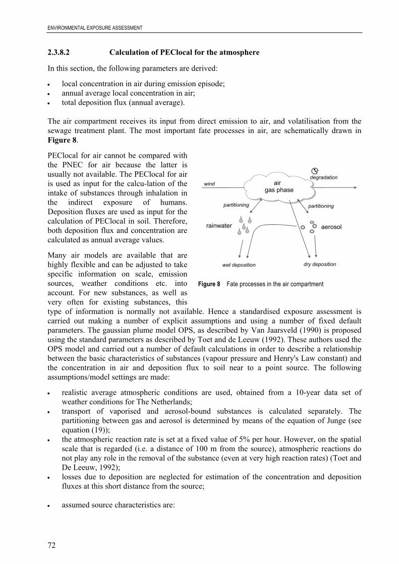
ENVIRONMENTAL EXPOSURE ASSESSMENT
72
2.3.8.2 Calculation of PEClocal for the atmosphere
In this section, the following parameters are derived:
• local concentration in air during emission episode;• annual average local concentration in air;• total deposition flux (annual average).
The air compartment receives its input from direct emission to air, and volatilisation from thesewage treatment plant. The most important fate processes in air, are schematically drawn inFigure 8.
PEClocal for air cannot be compared withthe PNEC for air because the latter isusually not available. The PEClocal for airis used as input for the calcu-lation of theintake of substances through inhalation inthe indirect exposure of humans.Deposition fluxes are used as input for thecalculation of PEClocal in soil. Therefore,both deposition flux and concentration arecalculated as annual average values.
Many air models are available that arehighly flexible and can be adjusted to takespecific information on scale, emissionsources, weather conditions etc. intoaccount. For new substances, as well asvery often for existing substances, thistype of information is normally not available. Hence a standardised exposure assessment iscarried out making a number of explicit assumptions and using a number of fixed defaultparameters. The gaussian plume model OPS, as described by Van Jaarsveld (1990) is proposedusing the standard parameters as described by Toet and de Leeuw (1992). These authors used theOPS model and carried out a number of default calculations in order to describe a relationshipbetween the basic characteristics of substances (vapour pressure and Henry's Law constant) andthe concentration in air and deposition flux to soil near to a point source. The followingassumptions/model settings are made:
• realistic average atmospheric conditions are used, obtained from a 10-year data set ofweather conditions for The Netherlands;
• transport of vaporised and aerosol-bound substances is calculated separately. Thepartitioning between gas and aerosol is determined by means of the equation of Junge (seeequation (19));
• the atmospheric reaction rate is set at a fixed value of 5% per hour. However, on the spatialscale that is regarded (i.e. a distance of 100 m from the source), atmospheric reactions donot play any role in the removal of the substance (even at very high reaction rates) (Toet andDe Leeuw, 1992);
• losses due to deposition are neglected for estimation of the concentration and depositionfluxes at this short distance from the source;
• assumed source characteristics are:
air
aerosolrainwater
gas phase
partitioning
wind
wet deposition
partitioning
dry deposition
degradation
Figure 8 Fate processes in the air compartment
ENVIRONMENTAL EXPOSURE ASSESSMENT
73
- source height: 10 meters, representing the height of buildings in which production,processing or use take place;
- heat content of emitted gases: 0; this assumes there is no extra plume rise caused by excessheat of vapours compared to the outdoor temperature;
- source area: 0 meter; representing an ideal point source which is obviously not alwayscorrect but which is an acceptable choice;
• calculated concentrations are long-term averages.
The concentration in air at a distance of 100 meters from the point source is estimated. Thisdistance is chosen to represent the average distance between the emission source and the borderof the industrial site. The deposition flux of gaseous and aerosol-bound substances is estimatedanalogous to the estimation of atmospheric concentrations by means of an estimation schemeand with help of the OPS model. The deposition flux to soil is averaged over a circular areaaround the source, with a radius of 1000 m to represent the local agricultural area. Depositionvelocities are used for three different categories:
• dry deposition of gas/vapour: estimated at 0.01 cm/s;• wet deposition of gas/vapour: determined with the OPS model;• dry and wet deposition of aerosol particles; determined within the OPS model using an
average particle size distribution.
Based on the assumptions and model settings as listed above, calculations with the original OPS-model were performed for both gaseous and aerosol substances (Toet and de Leeuw, 1992).These calculations were only carried out for a source strength of 1 g/s, as it was proven thatconcentrations and deposition fluxes are proportional to the source strength. From thesecalculations it was concluded that local atmospheric concentrations are largely independent ofthe physical-chemical properties of the compounds. Hence, once the emission from a pointsource is known, the concentration at 100 meter from the source can be estimated from a simplelinear relationship.
In the calculation of PEClocal for air both emission from a point source as well as the emissionfrom a STP is taken into account. The concentration on the regional scale (PECregional) is usedas background concentration and therefore, summed to the local concentration. The STP isassumed as a point source and the concentration of the chemical is calculated at a 100 m distancefrom it. The maximum from the two concentrations (direct and via STP) is used as the PEClocal:
( )air air air airClocal = Elocal , Estp Cstdmax • (40)
air,ann airClocal = Clocal Temission•
365(41)

ENVIRONMENTAL EXPOSURE ASSESSMENT
74
Explanation of symbols
Elocalair local direct emission rate to air during episode [kg.d-1] eq. (5)Estpair local indirect emission to air from STP during episode [kg.d-1] eq. (35)Cstdair concentration in air at source strength of 1 kg.d-1 [mg.m-3] 2.78.10-4
Temission number of days per year that the emission takes place [d.year-1] App. IBClocalair local concentration in air during emission episode [mg.m-3]Clocalair,ann annual average concentration in air, 100 m from point source [mg.m-3]
air,ann air,ann airPEClocal = Clocal + PECregional (42)
Explanation of symbols
Clocalair,ann annual average local concentration in air [mg.m-3] eq. (40)PECregionalair regional concentration in air [mg.m-3] 2.3.8.7PEClocalair,ann annual average predicted environmental conc. in air [mg.m-3]
The calculation of deposition flux is slightly more complex because of the dependence of thedeposition flux on the fraction of the substance that is associated with the aerosols. In calculatingthe deposition flux, the emissions from the two sources (direct and STP) are summed:
( ) ( ) DEPstd Fass- + DEPstd Fass Estp + Elocal = DEPtotal gasaeraeraerairair ••• )(1 (43)
annDEPtotal = DEPtotal Temission•
365 (44)
Explanation of symbols
Elocalair local direct emission rate to air during emission episode [kg.d-1] eq. (5)Estpair local indirect emission to air from STP during episode [kg.d-1] eq. (35)Fassaer fraction of the substance bound to aerosol [-] eq. (19)DEPstdaer standard deposition flux of aerosol-bound compounds at a
source strength of 1 kg.d-1 [mg.m-2.d-1] 1.10-2 DEPstdgas deposition flux of gaseous compounds as a function
of Henry's Law constant, at a source strength of 1 kg.d-1 [mg.m-2.d-1]10logHENRY ≤ -2: 5.10-4
-2 < 10logHENRY ≤ 2: 4.10-4
10logHENRY > 2: 3.10-4
Temission number of days per year that the emission takes place [d.yr-1] App. IBDEPtotal total deposition flux during emission episode [mg.m-2.d-1]DEPtotalann annual average total deposition flux [mg.m-2.d-1]

ENVIRONMENTAL EXPOSURE ASSESSMENT
75
2.3.8.3 Calculation of PEClocal for the aquatic compartment
In this section, the following parameters are derived:
• local concentration in surface water during emission episode;• annual average local concentration in surface water.
The effluent of the sewage treatment plant is diluted into the surface water. Figure 9 shows themost important fate processes of the aquatic compartment. For the calculations, the followingassumptions are made:
• complete mixing of the effluentin surface water is assumed as arepresentative exposure situationfor the aquatic eco-system;
• for the first approach in the localassessments, volatilisation,degradation, and sedimentationare ignored because of the shortdistance between the point ofeffluent discharge and theexposure location.
The calculation of the PEClocal for theaquatic compartment involves severalsequential steps (see also Figure 9). Itincludes the calculation of thedischarge concentration of a STP to awater body, dilution effects andremoval from the aqueous medium byadsorption to suspended matter.
Dilution in the receiving surface water and adsorption to suspended matter
The distance from the point of discharge where complete mixing may be assumed will varybetween different locations. A fixed dilution factor may be applied. Dilution factors aredependent on flow rates and the industry specific discharge flow. Due to the different seasonal,climatic and geographical conditions in the Member States, those dilution factors may vary overwide ranges. They have been reported in a range from 1 (e.g. dry riverbeds in summer) up to100,000 (de Greef and de Nijs, 1990). The dilution factor is generally linked to the releasescenario of the use category. For example, for consumer products an average dilution factor forsewage from municipal treatment plants of 10 is recommended. This is also regarded as a defaultdilution value for other types of substances if no specific data are available.
When a substance is released to surface water predominately as particles (e.g. as precipitates orincorporated in small material pieces – see Section 2.3.3.5) this may lead to overestimation ofPECsurface water and underestimation of PECsediment. If this is expected to occur it should beconsidered in the further evaluation (e.g. when comparing PEC with monitoring data and in therisk characterisation).
In certain circumstances, it may be possible to identify specific emission points which wouldallow the use of more precise information regarding the available distribution and fate processes.
STP
dilut
ion
partitioningsuspended
matter
volatilisation
degradationsedimentation/resuspension
Figure 9 Fate processes in surface water
ENVIRONMENTAL EXPOSURE ASSESSMENT
76
Such site-specific assessments should only be used when it is known that all the emissionsemanating from the particular point in the life-cycle e.g. manufacture, arise from a limitednumber of specific and identifiable sites. In these circumstances each specific point of releasewill need to be assessed individually. If it is not possible to make this judgement, then the defaultassumptions should be applied. In site-specific assessments, due account can be taken of the truedilution available to the given emission as well as the impact of degradation, volatilisation, etc.in the derivation of the PEC. Normally, only dilution and adsorption to suspended sediment needto be considered but site-specific conditions may indicate that local distribution models can beused.
It must be noted that with the assumption of complete mixing of the effluent in the surface waterno account is taken of the fact that in reality in the mixing zone higher concentrations will occur.For situations with relatively low dilution factors this mixing-zone effect can be accepted. Forsituations with very high dilution factors, however, the mixing zones may be very long and theoverall area that is impacted by the effluent before it is completely mixed can be verysubstantial. Therefore, in case of site-specific assessments the dilution factor that is applied forcalculation of the local concentration in surface water should not be greater than 1000.
If no measured data are available on the partition coefficient between suspended matter andwater, Kpsusp, it can be estimated from the Koc of the substance, determined for other sorbentslike soil or sediments (Section 2.3.5) by taking into account different organic carbon contents ofthe media.
For some substances it may be possible that PECs are calculated in water which are in excess ofthe water solubility. These results need to be interpreted carefully on a case-by-case basis. Theconcentration in surface water will not be corrected, but the result needs to be flagged. The PEChas to be interpreted based on the effects found in the aquatic toxicity tests.
In a situation where a substance is released through several point sources into the same river, theresulting cumulative concentration may in a first approach be estimated by assuming it to bereleased from one point source. If this PEC leads to “concern” then refined approaches may beused, such as river flow models, e.g. OECD (1992a) which address the specific emission patternas well as river parameters.
The local concentration in surface water is calculated as follows.
DILUTION SUSP Kp + Clocal = Clocal
watersusp
effwater
••• )101( 6-(45)
Explanation of symbols
Clocaleff concentration of the substance in the STP effluent [mg.l-1] eq. (33)Kpsusp solids-water partitioning coefficient of suspended matter [l.kg-1] eq. (23)SUSPwater concentration of suspended matter in the river [mg.l-1] 15DILUTION dilution factor [-] 10Clocalwater local concentration in surface water during emission episode [mg.l-1]

ENVIRONMENTAL EXPOSURE ASSESSMENT
77
When considering the available dilution, account should be taken of the fluctuating flow-rates oftypical receiving waters. The low-flow rate (or 10th percentile) should always be used. Whereonly average flows are available, the flow for dilution purposes should be estimated as one thirdof this average. When a site-specific assessment is appropriate, the actual dilution factor aftercomplete mixing can be calculated from the flow rate of the river and the effluent discharge rate(this approach should only be used for rivers, not for estuaries or lakes):
DILUTION = EFFLUENT + FLOWEFFLUENT
stp
stp(46)
Explanation of symbols
EFFLUENTstp effluent discharge rate of stp [l.d-1] eq. (34)FLOW flow rate of the river [l.d-1] data setDILUTION dilution factor at the point of complete mixing [-] (max. = 1000)
For indirect human exposure and secondary poisoning, an annual average concentration insurface water is calculated:
water,ann waterClocal = Clocal Temission•
365(47)
Explanation of symbols
Clocalwater local concentration in surface water during emission episode [mg.l-1] eq. (45)Temission number of days per year that the emission takes place [d.yr-1] App. IBClocalwater,ann annual average local concentration in surface water [mg.l-1]
The concentration at the regional scale (PECregionalwater) is used as background concentrationfor the local scale. Therefore, these concentrations are summed:
water water waterPEClocal = Clocal + PECregional (48)
water,ann water,ann waterPEClocal = Clocal + PECregional (49)
Explanation of symbols
Clocalwater local concentration in surface water during episode [mg.l-1] eq. (45)Clocalwater,ann annual average concentration in surface water [mg.l-1] eq. (47)PECregionalwater regional concentration in surface water [mg.l-1] 2.3.8.7PEClocalwater predicted environmental concentration during episode [mg.l-1]PEClocalwater,ann annual average predicted environmental concentration [mg.l-1]

ENVIRONMENTAL EXPOSURE ASSESSMENT
78
2.3.8.4 Calculation of PEClocal for sediment
In this section, the following parameter is derived:
• local concentration in sediment during the emission episode.
PEClocal for sediment can be compared to the PNEC for sediment dwelling organisms. Theconcentration in freshly deposited sediment is taken as the PEC for sediment, therefore, theproperties of suspended matter are used. The concentration in bulk sediment can be derived fromthe corresponding water body concentration, assuming a thermodynamic partitioning equilibrium(see also Di Toro et al., 1991):
sedsusp-water
suspwaterPEClocal = K
RHO PEClocal • • 1000 (50)
Explanation of symbols
PEClocalwater concentration in surface water during emission episode [mg.l-1] eq. (48)Ksusp-water suspended matter-water partitioning coefficient [m3.m-3] eq. (24)RHOsusp bulk density of suspended matter [kg.m-3] eq. (18)PEClocalsed predicted environmental concentration in sediment [mg.kg-1]
Highly adsorptive substances may not be considered adequately with the approach describedabove, as they are often not in equilibrium distribution between water and suspended matterbecause of their cohesion to the suspended matter; however they may be desorbed after ingestionby benthic or soil organisms.
In the case when release to the surface water predominately occurs as particles (see Section2.3.8.3) this calculation may underestimate the sediment concentration. If this is expected tooccur it should be considered in the further evaluation (e.g. when comparing PEC withmonitoring data and in the risk characterisation).
2.3.8.5 Calculation of PEClocal for the soil compartment
In this section, the following parameters are derived:
• local concentration in agricultural soil (averaged over a certain time period);• local concentration in grassland (averaged over a certain time period);• percentage of steady-state situation (to indicate persistency).
Exposure assessment for the soil compartment is important with respect to exposure of terrestrialorganisms. Furthermore, crops are grown on agricultural soils for human consumption, andcattle, producing meat and milk, are grazing on grasslands. Figure 10 shows the most importantfate processes in the soil compartment.
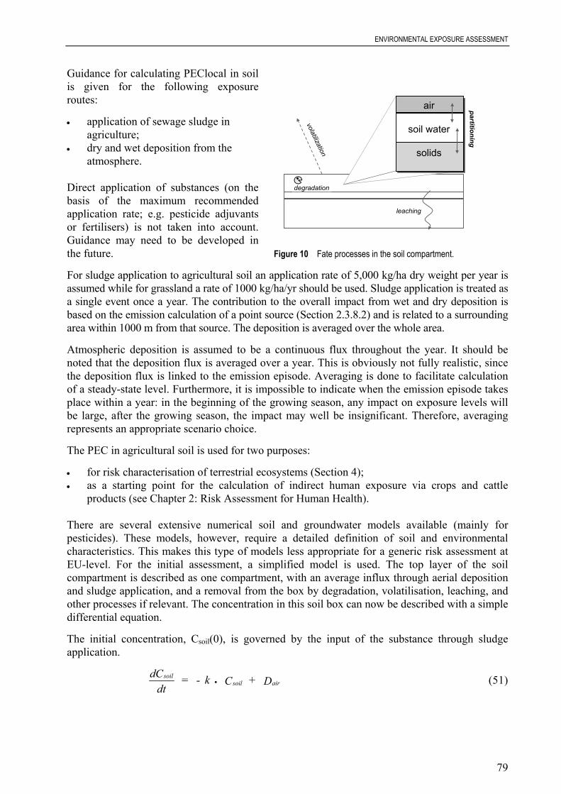
ENVIRONMENTAL EXPOSURE ASSESSMENT
Guidance for calculating PEClocal in soilis given for the following exposureroutes:
• application of sewage sludge inagriculture;
• dry and wet deposition from theatmosphere.
Direct application of substances (on thebasis of the maximum recommendedapplication rate; e.g. pesticide adjuvantsor fertilisers) is not taken into account.Guidance may need to be developed inthe future.
For sludge application to agricultural soil an application rate of 5,000 kg/ha dry weight per year isassumed while for grassland a rate of 1000 kg/ha/yr should be used. Sludge application is treated asa single event once a year. The contribution to the overall impact from wet and dry deposition isbased on the emission calculation of a point source (Section 2.3.8.2) and is related to a surroundingarea within 1000 m from that source. The deposition is averaged over the whole area.
Atmospheric deposition is assumed to be a continuous flux throughout the year. It should benoted that the deposition flux is averaged over a year. This is obviously not fully realistic, sincethe deposition flux is linked to the emission episode. Averaging is done to facilitate calculationof a steady-state level. Furthermore, it is impossible to indicate when the emission episode takesplace within a year: in the beginning of the growing season, any impact on exposure levels willbe large, after the growing season, the impact may well be insignificant. Therefore, averagingrepresents an appropriate scenario choice.
The PEC in agricultural soil is used for two purp
• for risk characterisation of terrestrial ecosys• as a starting point for the calculation of and cattle
products (see Chapter 2: Risk Assessment f
There are several extensive numerical soil a mainly forpesticides). These models, however, require ironmentalcharacteristics. This makes this type of models essment atEU-level. For the initial assessment, a simpl of the soilcompartment is described as one compartment, depositionand sludge application, and a removal from the ching, andother processes if relevant. The concentration in th a simpledifferential equation.
The initial concentration, Csoil(0), is governed gh sludgeapplication.
soilsoil air
dCdt
= - k C + D•
air
soil water
solids
leaching
degradation
volatilization
partitioning
Figure 10 Fate processes in the soil compartment.
oses:
tems (Section 4); indirect human exposure via crops or Human Health).
nd groundwater models available (a detailed definition of soil and env less appropriate for a generic risk assified model is used. The top layer with an average influx through aerial box by degradation, volatilisation, lea this soil box can now be described wi
by the input of the substance throu
79
(51)

ENVIRONMENTAL EXPOSURE ASSESSMENT
80
Explanation of symbols
Dair aerial deposition flux per kg of soil [mg.kg-1.d-1] eq. (52)t time [d]k first order rate constant for removal from top soil [d-1] eq. (56)Csoil concentration in soil [mg.kg-1]
In the formula above, the aerial deposition flux is used in mg substance per kg of soil per day.Dair can be derived by converting the total deposition flux (DEPtotalann) as follows:
airann
soil soilD = DEPtotal
DEPTH RHO•
(52)
Explanation of symbols
DEPtotalann annual average total deposition flux [mg.m-2.d-1] eq. (44)DEPTHsoil mixing depth of soil [m] Table 11RHOsoil bulk density of soil [kg.m-3] eq. (18)Dair aerial deposition flux per kg of soil [mg.kg-1.d-1]
The differential equation (51) has an analytical solution, given by:
e C - kD -
kD = t C t k -
soilairair
soil •
(0))( (53)
With this equation, the concentration can becalculated at each moment in time, when theinitial concentration in that year is known.
Accumulation of the substance may occurwhen sludge is applied over consecutiveyears. This is illustrated in Figure 11. As arealistic worst-case exposure scenario, it isassumed that sludge is applied for 10consecutive years. To indicate for potentialpersistency of the substance, the percentageof the steady-state situation is calculated. Asshown in Figure 11, the concentration in soilis not constant in time.
The concentration will be high just aftersludge application (in the beginning of thegrowth season), and lower at the end of theyear due to removal processes. Therefore, forexposure of the endpoints, the concentrationneeds to be averaged over a certain time period. Different averaging times should be consideredfor these endpoints: for the ecosystem a period of 30 days after application of sludge is used. In
Con
cent
ratio
n (%
of i
nitia
l)
time (year)0
0
40
20
60
80
100
120
140
160
1 2 3 4
Figure 11 Accumulation in soil due to several years of sludge application
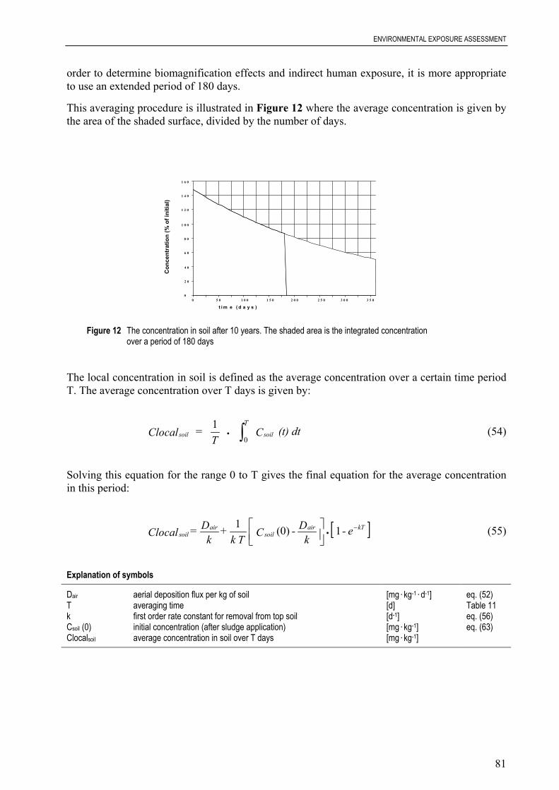
ENVIRONMENTAL EXPOSURE ASSESSMENT
81
0 5 0 1 0 0 1 5 0 2 0 0 2 5 0 3 0 0 3 5 0
t i m e ( d a y s )
1 6 0
1 4 0
1 2 0
1 0 0
8 0
6 0
4 0
2 0
0
Con
cent
ratio
n (%
of i
nitia
l)
Figure 12 The concentration in soil after 10 years. The shaded area is the integrated concentrationover a period of 180 days
order to determine biomagnification effects and indirect human exposure, it is more appropriateto use an extended period of 180 days.
This averaging procedure is illustrated in Figure 12 where the average concentration is given bythe area of the shaded surface, divided by the number of days.
The local concentration in soil is defined as the average concentration over a certain time periodT. The average concentration over T days is given by:
soil soilClocal = T
C (t) dtT10
• ∫ (54)
Solving this equation for the range 0 to T gives the final equation for the average concentrationin this period:
[ ]kTairsoil
airsoil e-
kD - C
T k +
kD = Clocal −
•
1(0)1 (55)
Explanation of symbols
Dair aerial deposition flux per kg of soil [mg.kg-1.d-1] eq. (52)T averaging time [d] Table 11k first order rate constant for removal from top soil [d-1] eq. (56)Csoil (0) initial concentration (after sludge application) [mg.kg-1] eq. (63)Clocalsoil average concentration in soil over T days [mg.kg-1]
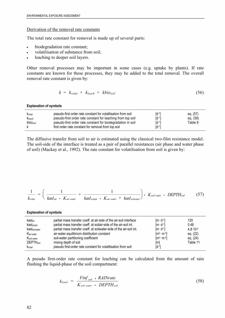
ENVIRONMENTAL EXPOSURE ASSESSMENT
82
Derivation of the removal rate constants
The total rate constant for removal is made up of several parts:
• biodegradation rate constant;• volatilisation of substance from soil;• leaching to deeper soil layers.
Other removal processes may be important in some cases (e.g. uptake by plants). If rateconstants are known for these processes, they may be added to the total removal. The overallremoval rate constant is given by:
k = kvolat + kleach + kbiosoil (56)
Explanation of symbols
kvolat pseudo-first order rate constant for volatilisation from soil [d-1] eq. (57)kleach pseudo-first order rate constant for leaching from top soil [d-1] eq. (58)kbiosoil pseudo-first order rate constant for biodegradation in soil [d-1] Table 8k first order rate constant for removal from top soil [d-1]
The diffusive transfer from soil to air is estimated using the classical two-film resistance model.The soil-side of the interface is treated as a pair of parallel resistances (air phase and water phaseof soil) (Mackay et al., 1992). The rate constant for volatilisation from soil is given by:
1 1 1volat air air-water soilair air-water soilwater
soil-water soilk
= kasl K
+ kasl K + kasl
K DEPTH• •
• •
(57)
Explanation of symbols
kaslair partial mass transfer coeff. at air-side of the air-soil interface [m.d-1] 120kaslsoilair partial mass transfer coeff. at soilair-side of the air-soil int. [m.d-1] 0.48kaslsoilwater partial mass transfer coeff. at soilwater-side of the air-soil int. [m.d-1] 4.8⋅10-5
Kair-water air-water equilibrium distribution constant [m3.m-3] eq. (22)Ksoil-water soil-water partitioning coefficient [m3.m-3] eq. (24)DEPTHsoil mixing depth of soil [m] Table 11kvolat pseudo first-order rate constant for volatilisation from soil [d-1]
A pseudo first-order rate constant for leaching can be calculated from the amount of rainflushing the liquid-phase of the soil compartment:
leachsoil
soil-water soilk =
Finf RAINrateK DEPTH
•
•
(58)

ENVIRONMENTAL EXPOSURE ASSESSMENT
83
Explanation of symbols
Finfsoil fraction of rain water that infiltrates into soil [-] 0.25RAINrate rate of wet precipitation (700 mm/year) [m.d-1] 1.92⋅10-3
Ksoil-water soil-water partitioning coefficient [m3.m-3] eq. (24)DEPTHsoil mixing depth of soil [m] Table 11kleach pseudo first-order rate constant for leaching from soil layer [d-1]
Derivation of the initial concentration after 10 years of sludge application
As a realistic worst-case assumption for exposure, it is assumed that sludge application takesplace for 10 consecutive years. To be able to calculate the concentration in this year averagedover the time period T (equation (55)), an initial concentration in this year needs to be derived.For this purpose, the contributions of deposition and sludge applications are consideredseparately.
The concentration due to 10 years of continuous deposition only, is given by applying equation(53) with an initial concentration of zero and 10 years of input:
e k
D - k
D = Cdep k -airair soil
•••
10 36510 (0) (59)
For sludge application, the situation is more complicated as this is not a continuous process. Theconcentration just after the first year of sludge application is given by:
soil sludge sludge
soil soilCsludge = C APPL
DEPTH RHO1 (0)•
•
(60)
Explanation of symbols
Csludge concentration in dry sewage sludge [mg.kg-1] eq. (36)APPLsludge dry sludge application rate [kg.m-2.yr-1] Table 11DEPTHsoil mixing depth of soil [m] Table 11RHOsoil bulk density of soil [kg.m-3] eq. (18)Csludgesoil 1 (0) concentration in soil due to sludge in first year at t=0 [mg.kg-1]
The fraction of the substance that remains in the top soil layer at the end of a year is given by:
Facc = e- k365 (61)
Explanation of symbols
k first order rate constant for removal from top soil [d-1] eq. (56)Facc fraction accumulation in one year [-]

ENVIRONMENTAL EXPOSURE ASSESSMENT
84
At the end of each year, a fraction Facc of the initial concentration remains in the top-soil layer.The initial concentration after 10 applications of sludge is given by:
[ ]soil soil n = nCsludge = Csludge + Facc 10 1 1
9(0) (0) 1• ∑ (62)
The sum of both the concentration due to deposition and sludge is the initial concentration inyear 10:
soil soil soil C = Cdep + Csludge 10 10 10(0) (0) (0) (63)
This initial concentration can be used in equation (54) to calculate the average concentration insoil over a certain time period.
Indicating persistency of the substance in soil
Ten consecutive years of accumulation may not be sufficient for some substances to reach asteady-state situation. These substances may accumulate for hundreds of years. To indicatepotential problems of persistency in soil, the fraction of the steady-state concentration can bederived:
Fst - st = C C
soil
soil
10 (0)(0)∞
(64)
Explanation of symbols
Csoil 10 (0) initial concentration after 10 years [mg.kg-1] eq. (63)Csoil ∞ (0) initial concentration in steady-state situation [mg.kg-1] eq. (65)Fst-st fraction of steady-state in soil achieved [-]
The initial concentration in the steady-state year is given by:
soil air
soil C = Dk
+ Csludge - Facc∞ •(0) (0) 1
11 (65)
Explanation of symbols
Dair aerial deposition flux per kg of soil [mg.kg-1.d-1] eq. (52)k first order rate constant for removal from top soil [d-1] eq. (56)Facc fraction accumulation in one year [-] eq. (61)Csludgesoil 1 (0) concentration in soil due to sludge in first year at t=0 [mg.kg-1] eq. (60)Csoil∞(0) initial concentration in steady-state situation [mg.kg-1]

ENVIRONMENTAL EXPOSURE ASSESSMENT
85
Calculation of PEClocalsoil
For soil, three different PECs are calculated, for different endpoints (Table 11).
Table 11 Characteristics of soil and soil-use for the three different endpoints
Depth of soilcompartment
Averaging time Rate of sludge application Endpoint
[m] [days] [kgdwt.m-2.year-1]
PEClocalsoil 0.20 30 0.5 terrestrial ecosystem
PEClocalagr. soil 0.20 180 0.5 crops for human consumption
PEClocalgrassland 0.10 180 0.1 grass for cattle
The “depth of soil” represents the depth range for the top soil layer which is of interest. Thedepth of 20 cm is taken because this range usually has a high root density of crops, andrepresents the ploughing depth. For grassland, the depth is less since grasslands are notploughed. The averaging period of 180 days for crops is chosen as a representative growingperiod for crops. For grassland this period represents a reasonable assumption for the period thatcattle is grazing on the field. For the ecosystem a period of 30 days is taken as a relevant timeperiod with respect to chronic exposure of soil organisms.
The concentration at the regional scale is used as background concentration for the local scale.For this purpose, the concentration in unpolluted soil needs to be applied (“natural soil”, onlyinput through deposition). Otherwise, sludge application is taken into account twice.
soil soil natural soilPEClocal = Clocal + PECregional (66)
Explanation of symbols
Clocalsoil local concentration in soil [mg.kg-1] eq. (54)PECregionalnatural soil regional concentration in natural soil [mg.kg-1] 2.3.8.7PEClocalsoil predicted environmental conc. in soil [mg.kg-1]
The equation for deriving the concentration in the pore water is:
soil, porewsoil soil
soil-waterPEClocal = PEClocal RHO
K •
• 1000(67)
Explanation of symbols
PEClocalsoil predicted environmental conc. in soil [mg.kg-1] eq. (66)Ksoil-water soil-water partitioning coefficient [m3.m-3] eq. (24)RHOsoil bulk density of wet soil [kg.m-3] eq. (18)PEClocalsoil,porew predicted environmental conc. in porewater [mg.l-1]
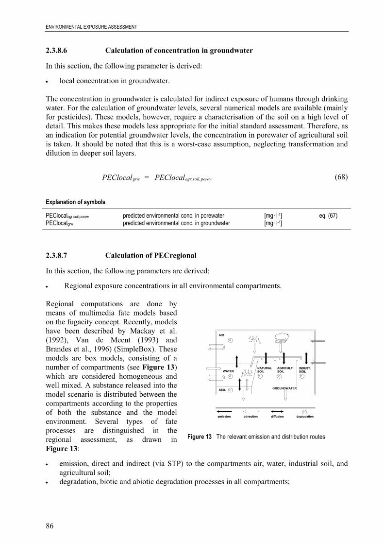
ENVIRONMENTAL EXPOSURE ASSESSMENT
86
2.3.8.6 Calculation of concentration in groundwater
In this section, the following parameter is derived:
• local concentration in groundwater.
The concentration in groundwater is calculated for indirect exposure of humans through drinkingwater. For the calculation of groundwater levels, several numerical models are available (mainlyfor pesticides). These models, however, require a characterisation of the soil on a high level ofdetail. This makes these models less appropriate for the initial standard assessment. Therefore, asan indication for potential groundwater levels, the concentration in porewater of agricultural soilis taken. It should be noted that this is a worst-case assumption, neglecting transformation anddilution in deeper soil layers.
grw agr.soil, porewPEClocal = PEClocal (68)
Explanation of symbols
PEClocalagr.soil,porew predicted environmental conc. in porewater [mg.l-1] eq. (67)PEClocalgrw predicted environmental conc. in groundwater [mg.l-1]
2.3.8.7 Calculation of PECregional
In this section, the following parameters are derived:
• Regional exposure concentrations in all environmental compartments.
Regional computations are done bymeans of multimedia fate models basedon the fugacity concept. Recently, modelshave been described by Mackay et al.(1992), Van de Meent (1993) andBrandes et al., 1996) (SimpleBox). Thesemodels are box models, consisting of anumber of compartments (see Figure 13)which are considered homogeneous andwell mixed. A substance released into themodel scenario is distributed between thecompartments according to the propertiesof both the substance and the modelenvironment. Several types of fateprocesses are distinguished in theregional assessment, as drawn inFigure 13:
• emission, direct and indirect (via STP) to the compartments air, water, industrial soil, andagricultural soil;
• degradation, biotic and abiotic degradation processes in all compartments;
emission advection diffusion degradation
AIR
WATER
SED.
SOILNATURAL
SOILAGRICULT.
SOILINDUST.
GROUNDWATER
AIR
Figure 13 The relevant emission and distribution routes
ENVIRONMENTAL EXPOSURE ASSESSMENT
87
• diffusive transport, as e.g. gas absorption and volatilisation. Diffusive mass transfer betweentwo compartments goes both ways, the net flow may be either way, depending on theconcentration in both compartments;
• advective transport, as e.g. deposition, run-off, erosion. In the case of advective transport, asubstance is carried from one compartment into another by a carrier that physically flowsfrom one compartment into the other. Therefore, advective transport is strictly one-way.
Substance input to the model is regarded as continuous and equivalent to continuous diffuseemission. The results from the model are steady-state concentrations, which can be regarded asestimates of long-term average exposure levels. The fact that a steady state between thecompartments is calculated, does not imply that the compartment to which the emission takesplace is of no importance.
In a Mackay-type level III model, the distribution and absolute concentrations may highlydepend upon the compartment of entry.
Advective import and export (defined as inflow from outside the model or outflow from themodel environment) can be very important for the outcome of both regional and local modelcalculations. Therefore, the concentration of a substance at the “border” of the region must betaken into account. This is defined as the background concentration of a substance. Thebackground concentration in a local model can be obtained from the outcome of the regionalmodel. For substances with many relatively small point sources, this background concentrationmay represent a significant addition to the concentration from a local source. The backgroundconcentration in the regional model has to be calculated using a similar box model of a largerscale, e.g. with the size of the European continent. In this continental model, however, it isassumed that no inflow of air and water across the boundaries occurs. Furthermore it is assumedthat all substance releases enter into this continental environment. The resulting steady-stateconcentrations are then used as transboundary or background concentrations in the regionalmodel. The continental and regional computations should thus be done in sequence. Figure 1visualises the relationship between the concentrations calculated for the different model scales.For both the regional and continental scale, the total emission amounts (through diffuse andpoint sources, summed over all stages of the life-cycle) are used.
For the PECregional calculation, in contrast to PEClocal, an average percentage connection rateto STPs should be included in the calculation. This leads to a more realistic estimation of thelikely background concentration on a regional scale. For the purposes of the generic regionalmodel, a STP connection rate of 80% (the EU average according to Appendix XII) will beassumed.
The results from the regional model should be interpreted with caution. The environmentalconcentrations are averages for the entire regional compartments (which were assumed wellmixed). Locally, concentrations may be much higher than these average values. Furthermore,there is a considerable degree of uncertainty due to the uncertainty in the determination of inputparameters (e.g. degradation rates, partitioning coefficients).
Model parameters for PECregional
When calculating the PECregional it is important which modelling parameters are chosen andwhat fraction of the total emissions is used as emission for the region. There are two differentpossibilities:

ENVIRONMENTAL EXPOSURE ASSESSMENT
88
• calculation of a PECregional on the basis of a standardised regional environment withagreed model parameters;
• calculation of a PECregional on the basis of country specific model parameters.
A standardised regional environment should be used for the first approach in the calculation ofPECregional. When more specific information is available on the location of production/emission sites, this information can be applied to refine the regional assessment. The secondapproach may sometimes result in a better estimation of the concentrations for a specificcountry. However, depending on the information on production site location, it will lead to anumber of different PEC values which makes a risk characterisation at EU level morecomplicated.
Calculations are performed for a densely populated area of 200.200 km with 20 millioninhabitants. Unless specific information on use or emission per capita is available, it is assumedthat 10% of the European production and use takes place within this area, i.e. 10% of theestimated emission is used as input for the region. The model parameters proposed for thisstandard region are given in Table 12. It should be noted that it is extremely difficult to selecttypical or representative values for a standard European region. Therefore, the rationale behindthe values of Table 12 is limited. Nevertheless, these values present a starting point for theregional scale assessments. Characterisation of the environmental compartments for theregional model should be done according to the values in Table 5.
Table 12 Proposed model parameters for regional model
Parameter Value in regional model
area of the regional system 4.104 km2
area fraction of water 0.03
area fraction of natural soil 0.60
area fraction of agricultural soil 0.27
area fraction of industrial/urban soil 0.10
mixing depth of natural soil 0.05 m
mixing depth of agricultural soil 0.2 m
mixing depth of industrial/urban soil 0.05 m
atmospheric mixing height 1000 m
depth of water 3 m
depth of sediment 0.03 m
fraction of the sediment compartment that is aerobic 0.10
average annual precipitation 700 mm.yr-1
wind speed 3 m.s-1
residence time of air 0.7 d
residence time of water 40 d
fraction of rain water infiltrating soil 0.25
fraction of rain water running off soil 0.25
EU average connection percentage to STP 80%
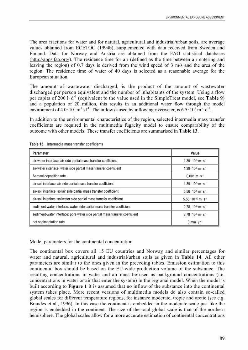
ENVIRONMENTAL EXPOSURE ASSESSMENT
89
The area fractions for water and for natural, agricultural and industrial/urban soils, are averagevalues obtained from ECETOC (1994b), supplemented with data received from Sweden andFinland. Data for Norway and Austria are obtained from the FAO statistical databases(http://apps.fao.org/). The residence time for air (defined as the time between air entering andleaving the region) of 0.7 days is derived from the wind speed of 3 m/s and the area of theregion. The residence time of water of 40 days is selected as a reasonable average for theEuropean situation.
The amount of wastewater discharged, is the product of the amount of wastewaterdischarged per person equivalent and the number of inhabitants of the system. Using a flowper capita of 200 l.d-1 (equivalent to the value used in the SimpleTreat model, see Table 9)and a population of 20 million, this results in an additional water flow through the modelenvironment of 4.0.106 m3.d-1. The inflow caused by inflowing riverwater, is 6.5.107 m3.d-1.
In addition to the environmental characteristics of the region, selected intermedia mass transfercoefficients are required in the multimedia fugacity model to ensure comparability of theoutcome with other models. These transfer coefficients are summarised in Table 13.
Table 13 Intermedia mass transfer coefficients
Parameter Value
air-water interface: air side partial mass transfer coefficient 1.39.10-3 m.s-1
air-water interface: water side partial mass transfer coefficient 1.39.10-5 m.s-1
Aerosol deposition rate 0.001 m.s-1
air-soil interface: air side partial mass transfer coefficient 1.39.10-3 m.s-1
air-soil interface: soilair side partial mass transfer coefficient 5.56.10-6 m.s-1
air-soil interface: soilwater side partial mass transfer coefficient 5.56.10-10 m.s-1
sediment-water interface: water side partial mass transfer coefficient 2.78.10-6 m.s-1
sediment-water interface: pore water side partial mass transfer coefficient 2.78.10-8 m.s-1
net sedimentation rate 3 mm.yr-1
Model parameters for the continental concentration
The continental box covers all 15 EU countries and Norway and similar percentages forwater and natural, agricultural and industrial/urban soils as given in Table 14. All otherparameters are similar to the ones given in the preceding tables. Emission estimation to thiscontinental box should be based on the EU-wide production volume of the substance. Theresulting concentrations in water and air must be used as background concentrations (i.e.concentrations in water or air that enter the system) in the regional model. When the model isbuilt according to Figure 1 it is assumed that no inflow of the substance into the continentalsystem takes place. More recent versions of multimedia models do also contain so-calledglobal scales for different temperature regions, for instance moderate, tropic and arctic (see e.g.Brandes et al., 1996). In this case the continent is embedded in the moderate scale just like theregion is embedded in the continent. The size of the total global scale is that of the northernhemisphere. The global scales allow for a more accurate estimation of continental concentrations
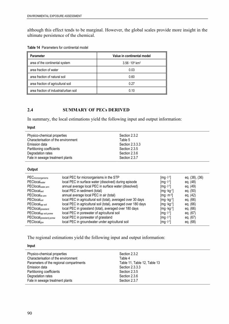
ENVIRONMENTAL EXPOSURE ASSESSMENT
90
although this effect tends to be marginal. However, the global scales provide more insight in theultimate persistence of the chemical.
Table 14 Parameters for continental model
Parameter Value in continental model
area of the continental system 3.56.106 km2
area fraction of water 0.03
area fraction of natural soil 0.60
area fraction of agricultural soil 0.27
area fraction of industrial/urban soil 0.10
2.4 SUMMARY OF PECs DERIVED
In summary, the local estimations yield the following input and output information:
Input
Physico-chemical properties Section 2.3.2Characterisation of the environment Table 5Emission data Section 2.3.3.3Partitioning coefficients Section 2.3.5Degradation rates Section 2.3.6Fate in sewage treatment plants Section 2.3.7
Output
PECmicroorganisms local PEC for microorganisms in the STP [mg.l-1] eq. (38), (36)PEClocalwater local PEC in surface water (dissolved) during episode [mg.l-1] eq. (48)PEClocalwater,ann annual average local PEC in surface water (dissolved) [mg.l-1] eq. (49)PEClocalsed local PEC in sediment (total) [mg.kg-1] eq. (50)PEClocalair,ann annual average local PEC in air (total) [mg.m-3] eq. (42)PEClocalsoil local PEC in agricultural soil (total), averaged over 30 days [mg.kg-1] eq. (66)PEClocalagr.soil local PEC in agricultural soil (total), averaged over 180 days [mg.kg-1] eq. (66)PEClocalgrassland local PEC in grassland (total), averaged over 180 days [mg.kg-1] eq. (66)PEClocalagr.soil,porew local PEC in porewater of agricultural soil [mg.l-1] eq. (67)PEClocalgrassland,porew local PEC in porewater of grassland [mg.l-1] eq. (67)PEClocalgrw local PEC in groundwater under agricultural soil [mg.l-1] eq. (68)
The regional estimations yield the following input and output information:
Input
Physico-chemical properties Section 2.3.2Characterisation of the environment Table 4Parameters of the regional compartments Table 11, Table 12, Table 13Emission data Section 2.3.3.3Partitioning coefficients Section 2.3.5Degradation rates Section 2.3.6Fate in sewage treatment plants Section 2.3.7
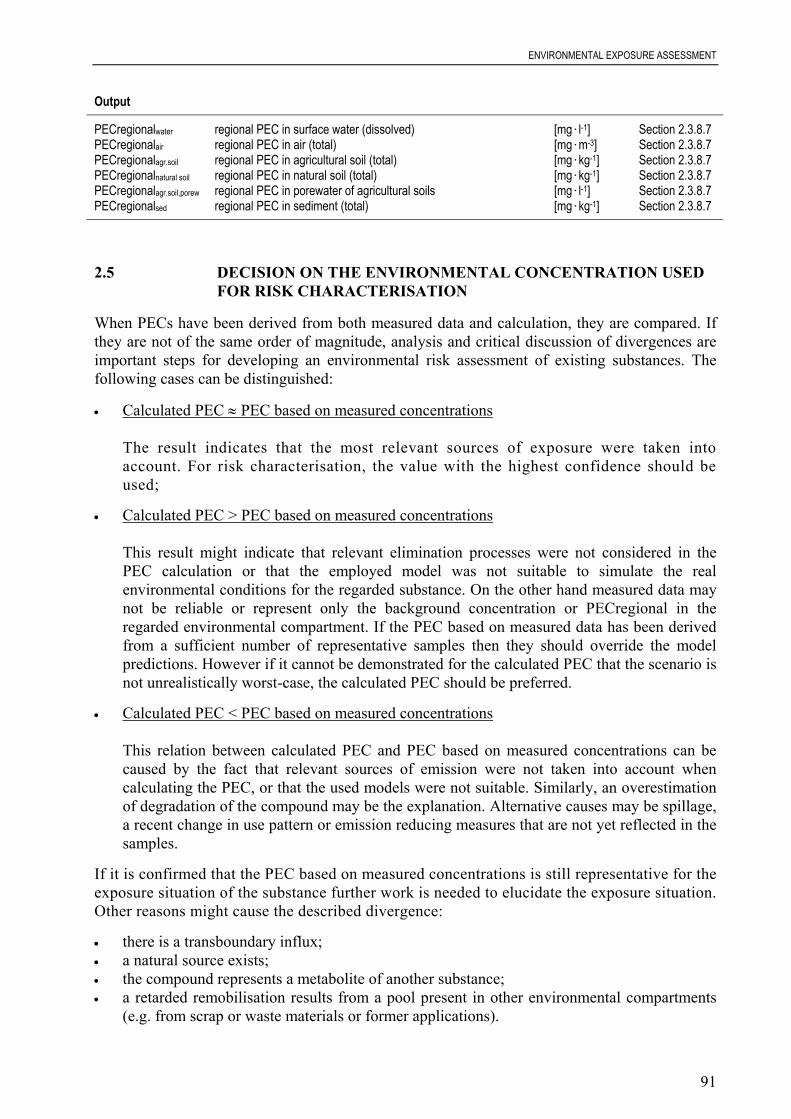
ENVIRONMENTAL EXPOSURE ASSESSMENT
91
Output
PECregionalwater regional PEC in surface water (dissolved) [mg.l-1] Section 2.3.8.7PECregionalair regional PEC in air (total) [mg.m-3] Section 2.3.8.7PECregionalagr.soil regional PEC in agricultural soil (total) [mg.kg-1] Section 2.3.8.7PECregionalnatural soil regional PEC in natural soil (total) [mg.kg-1] Section 2.3.8.7PECregionalagr.soil,porew regional PEC in porewater of agricultural soils [mg.l-1] Section 2.3.8.7PECregionalsed regional PEC in sediment (total) [mg.kg-1] Section 2.3.8.7
2.5 DECISION ON THE ENVIRONMENTAL CONCENTRATION USEDFOR RISK CHARACTERISATION
When PECs have been derived from both measured data and calculation, they are compared. Ifthey are not of the same order of magnitude, analysis and critical discussion of divergences areimportant steps for developing an environmental risk assessment of existing substances. Thefollowing cases can be distinguished:
• Calculated PEC ≈ PEC based on measured concentrations
The result indicates that the most relevant sources of exposure were taken intoaccount. For risk characterisation, the value with the highest confidence should beused;
• Calculated PEC > PEC based on measured concentrations
This result might indicate that relevant elimination processes were not considered in thePEC calculation or that the employed model was not suitable to simulate the realenvironmental conditions for the regarded substance. On the other hand measured data maynot be reliable or represent only the background concentration or PECregional in theregarded environmental compartment. If the PEC based on measured data has been derivedfrom a sufficient number of representative samples then they should override the modelpredictions. However if it cannot be demonstrated for the calculated PEC that the scenario isnot unrealistically worst-case, the calculated PEC should be preferred.
• Calculated PEC < PEC based on measured concentrations
This relation between calculated PEC and PEC based on measured concentrations can becaused by the fact that relevant sources of emission were not taken into account whencalculating the PEC, or that the used models were not suitable. Similarly, an overestimationof degradation of the compound may be the explanation. Alternative causes may be spillage,a recent change in use pattern or emission reducing measures that are not yet reflected in thesamples.
If it is confirmed that the PEC based on measured concentrations is still representative for theexposure situation of the substance further work is needed to elucidate the exposure situation.Other reasons might cause the described divergence:
• there is a transboundary influx;• a natural source exists;• the compound represents a metabolite of another substance;• a retarded remobilisation results from a pool present in other environmental compartments
(e.g. from scrap or waste materials or former applications).

ENVIRONMENTAL EXPOSURE ASSESSMENT
92
If the measured values have passed the procedure of critical statistical and geographicalevaluation, a high degree of confidence can be attributed to those data and they shall overwritethe calculated PECs. It is necessary to consider all environmental compartments when themeasurements and predictions are made otherwise the possibility of chance agreement may beoverlooked.

EFFECTS ASSESSMENT
93
3 EFFECTS ASSESSMENT
3.1 INTRODUCTION
The effects assessment comprises the following steps of the risk assessment procedure:
• hazard identification: The aim of the hazard identification is to identify the effects ofconcern. For existing substances and biocidal active substances and substances of concern inbiocidal products, the aim is also to review the classification of the substance while for newsubstances a proposal on classification is done;
• dose (concentration) - response (effect) assessment: At this step the predicted no effectconcentration (PNEC), shall, where possible, be determined.
For both steps of the effects assessment it is of high importance to evaluate the data with regardto their adequacy and completeness. The evaluation of adequacy shall address the quality andrelevance of data (see Section 3.2). The evaluation of data is of particular importance for existingsubstances as tests will often be available with non-standard organisms and/or non-standardisedmethods. It is suitable to start the effects assessment process with the evaluation of the availableecotoxicological data.
As stated in Section 1.2, the environmental compartments considered for the inland environmentare the aquatic and terrestrial ecosystem, top predators, microbial activity in a STP, and theatmosphere. This means that for each of these compartments a PNEC has to be derived. A PNECis regarded as a concentration below which an unacceptable effect will most likely not occur. Inprinciple, the PNEC is calculated by dividing the lowest short-term L(E)C50 or long-term NOECvalue by an appropriate assessment factor. The assessment factors reflect the degree ofuncertainty in extrapolation from laboratory toxicity test data for a limited number of species tothe 'real' environment. Assessment factors applied for long-term tests are smaller as theuncertainty of the extrapolation from laboratory data to the natural environment is reduced. Forthis reason long-term data are preferred to short-term data.
A detailed assessment of the environmental risk is often only feasible for the water compartment:for new substances the base-set consists of effect data for aquatic organisms only, while forexisting substances most of the available data will be for aquatic organisms. For biocides, thecore data set comprises effect data on aquatic organisms as well. Therefore, a more detaileddescription on deriving a PNECwater is described in Section 3.3. For an intermittent release ofsubstances, aquatic organisms may be exposed for only a short period. In these cases, short-termL(E)C50 values are used to derive a PNECwater, intermittent. This is described in Section 3.3.2.
The microbial activity in domestic and industrial STPs may be affected. Assessment factors toderive a PNECmicroorganisms are given in Section 3.4.
Probably for most compounds no data will be present for sediment-dwelling organisms.Appropriate test systems and standardised guidelines are still under development. Theequilibrium partitioning method is proposed as a screening method for derivation of a PNECsedto compensate for this lack of toxicity data. If sediment test results are available, the PNECsed isderived from these data by applying assessment factors (see Section 3.5).
Few toxicity data are also available for the soil compartment. Where such data are present, theywill normally include only test results from short-term studies. If test data are lacking, the
EFFECTS ASSESSMENT
94
equilibrium partitioning method can be used to derive a PNECsoil. Otherwise, assessment factorsare applied (see Section 3.6).
Biotic and abiotic effects, such as acidification, are addressed for the atmosphere. In view of thelack of suitable data and the fact that no adequate methods are available yet to assess both typesof effects, a provisional strategy is described in Section 3.7.
Standard assays of ecotoxicological effects usually provide information about the direct toxiceffects of a substance. Chemicals showing bioaccumulation and biomagnification may pose anadditional threat due to exposure of organisms higher in the food chain, e.g. top predators. Thisphenomenon is called 'secondary poisoning' and has to be addressed if a chemical fulfils severalcriteria, e.g. indication of a bioaccumulation potential. If this is the case, the oral intake of achemical via fish or worms (PECoralfish and PECoralworm) is compared to a PNEC for fish- orworm-eating mammals or birds. This approach is described in Section 3.8.
Knowledge on endocrine disrupting effects of some substances is presently under development.When substantial evidence on such effects is available, this should be taken into account on acase-by-case basis in the derivation of the PNEC for each compartment of relevance. Existingknowledge does not allow a more standardised approach for risk assessment of such substances.
It is recognised that experience with several of the described effects assessment methods islacking. Thus, assessments by use of these types of methods can be uncertain. However, themethods presented make it possible to identify if the compartment under consideration ispossibly “of concern” and whether further data, e.g. testing on relevant organisms for thatcompartment, should be obtained.
The environmental part of the risk assessment should contain some general reflection on themode of action of the chemical. Cross-reference to relevant sections in the human health partmay be important. For example when a chemical is found to have effects on gonad developmentin fish and similar effects have been observed in laboratory mammals. Identification ofsimilarities in the nature, intensity and time scale of effects between species, as well as in thesusceptibilities of different receptors, will allow a better understanding of the actual risk to theseorganisms to be obtained and help in the identification of issues of concern (IPCS, 2000).
3.2 EVALUATION OF DATA
3.2.1 Ecotoxicity data
During both steps of the effects assessment it is very important to evaluate data with regard totheir adequacy and completeness. This is particularly important for existing substances that havebeen extensively studied where there may be a number of test results available beyond the base-set. This section puts forward general guidelines on the evaluation of ecotoxicity data. The termadequacy is used here to cover the reliability of the available data and the relevance of that datafor environmental hazard and risk assessment.
EFFECTS ASSESSMENT
95
3.2.1.1 Completeness of data
New substances
For new substances data equivalent to those identified in Annex VII A to Directive 67/548 willbe available: the base-set. The base-set comprises short- term toxicity data for algae, Daphniaand fish for the aquatic compartment. Data for bacteria (respiration inhibition test) are also partof the base-set. These data are used for assessing the effects on microbial activity in a STP (seeSection 3.4). The base-set testing package contains relatively little data that are of relevance tothe terrestrial and atmospheric compartments: additional but nevertheless still limited data areobtained at level 1 and 2.
Existing substances
Availability of data for existing substances varies considerably. Regulation 793/93 requires thatfor priority substances at least the base-set data according to Annex VII A to Directive 67/548are provided before the risk assessment process begins. However, for many substances moreinformation will be available which can be used in the assessment.
The base-set ensures that short-term effects data are available for fish, Daphnia, algae andbacteria. Within a trophic level, a number of short-term investigations may also be available forseveral non-standard organisms. In addition, long-term toxicity investigations may be availablewith several species, standard organisms as well as non-standard organisms. These organismsshould be assigned to appropriate trophic levels for the derivation of the PNEC (see AppendixIV and Section 3.3.1). Multi-species tests, investigations with model ecosystems and semi-fieldtests, are rarely available for substances although in recent years more work has been done inthis area (Hill et al., 1994; Knacker and Morgan, 1994).
Active biocidal substances
The data requirements for active biocidal substances are laid down in Annex IIA and Annex IIIAof Directive 98/8. The core data requirements for biocides correspond to the base-set for newsubstances. However, depending on Product Type and intended use of the biocidal product,additional toxicity data may be required as described in the Technical Notes for Guidance insupport of Directive 98/8 on the placing of biocidal products on the market (TNsG on DataRequirements, 2000; http://ecb.jrc.it/biocides/).
3.2.1.2 Adequacy of data
The adequacy of a test data can be defined by two basic elements:
• reliability: covering the inherent quality of a test relating to test methodology and the waythat the performance and results of the test are described;
• relevance: covering the extent to which a test is appropriate for a particular hazard or riskassessment.
Only reliable, relevant data can be considered valid for use in the risk assessment.

EFFECTS ASSESSMENT
96
The assessment of data adequacy therefore involves:
• A review of individual data elements with respect to how the study is conducted and howthe results are interpreted; and,
• A critical selection (and rejection) of data in its proper context and in accordance with thepurpose of the assessment.
New substances and biocidal substances
The tests for new substances and biocidal substances must be carried out in accordance with theEU testing methods as laid down in Annex V to Directive 67/5483, or if no EU methods areavailable or they are not applicable, in accordance with internationally recognised guidelines,preferably those of the OECD (1993b). They must also be conducted in accordance with theprinciples of good laboratory practice as set out in Council Directive 87/18.
Existing substances
The risk assessment for existing substances starts with the collecting of all available informationby the manufacturers, importers, and the rapporteur. Any new tests carried out for riskassessments under Regulation 793/93 should be conducted according to the testing methods laiddown in Annex V to Directive 67/548, or if no EU methods are available or they are notapplicable, in accordance with internationally recognised guidelines, preferably those of theOECD (1993b). They must also be conducted following good laboratory practice according toDirective 87/18.
This information will probably contain data that have been generated prior to the requirements ofGLP being specified and prior to the standardisation of testing methods. However, these datamay be used for the risk assessment, if valid conclusions can be drawn from them. This meansthat the data, and the test methods used to generate them, must be evaluated in order todetermine whether they are of sufficient quality for use in risk assessment. Such an evaluationwill require the use of expert judgement, but the determination of data as being valid or not validmust be both justified and transparent. The requirements of the standardised test methods andGLP principles should be regarded as a reference when evaluating the available tests. Sufficientinformation must be available in order to allow a judgement on the reliability of a study to bemade.
Greater weight should normally be attached to studies carried out according to current methods(e.g. EU, OECD, or US EPA) (cf. Ahlers et al., 1992; OECD, 1998a). Criteria for data reliabilityrefer to accepted standards:
• a complete test report is available or the test has been described in sufficient detail and thetest procedure is in accordance with generally accepted standards. These data are consideredvalid and can be used for risk assessment;
• the validity of the data cannot be fully established or the test method differs in some respectsfrom the guidelines and the generally accepted scientific standards. Experts must decide ineach case whether the test result can be taken into consideration in the risk assessment or isregarded as not valid;
3 A complete listing of the EC Testing Methods as well as references to the relevant Directives and Official Journals
where they can be found are available in the ECB web page <http://ecb.jrc.it/testing-methods>. Some methods canbe downloaded from this site as well.
EFFECTS ASSESSMENT
97
• it is clearly evident that the data are not valid because critical pieces of information are notavailable and cannot be sourced retrospectively (e.g. it is not possible to establish theidentity of the test substance). These data are not considered to be valid for the riskassessment. However, they may be used as an aid in the design of an appropriate test.
In principle, the same criteria apply for tests reported in published literature. The amount ofinformation presented will provide the basis for deciding on the validity of a test result. Ingeneral, test results that have been reported in peer reviewed journals are preferred. High qualityreviews may be used as supporting information. Summaries or abstract publications may alsoprovide supporting data.
In cases where differing results from similar studies were obtained or an extensive data set isavailable for an individual species or a taxonomic group, it may be possible to use thedistribution of these data to draw general conclusions regarding the toxicity to that species ortaxon.
Results from field studies may also be available. These studies can vary widely in the nature ofthe experimental system: from indoor microcosms to outdoor macrocosms such as experimentalstreams (Hill et al., 1994). Field studies may provide a better insight into the toxic effects(including indirect effects) of chemicals, as well as factors affecting their routes of exposure (e.g.bioavailability, biodegradation). At present, there are no internationally accepted guidelines forfieldstudies. However, some general guidance has been laid down for the conduction of fieldstudies in aquatic ecosystems (SETAC, 1991; SETAC, 1992; Campbell et al., 1999; Posthuma etal., 2001).
Relevance of data
In order to evaluate the relevance of the available data, it is necessary to judge, inter alia, if theappropriate endpoints are studied under relevant conditions and if the substance tested isrepresentative of the substance being assessed. To be able to assess the latter it is essential thatthe substance is properly described and any significant impurities are identified.
Interpretation of data
In some cases the dose (concentration) - response (effect) relationship is not known, the durationof a test may be different from that of standard tests or the test parameters may not becomparable to those used in standard tests, for example investigations of photosynthesis, ofbehaviour, investigations on a cellular or a subcellular level. Expert judgement must therefore beused to determine whether such data can be interpreted for use in the assessment.
Short-term L(E)C50 and long-term NOEC values are used in the effects assessment. Guidance isgiven in Table 15 with respect to the derivation of L(E)C50 and NOEC values. However, resultsfrom ecotoxicological studies may also be reported using other conventions and expressions ofeffect. QSARs may be helpful in assessing long-term aquatic toxicity data from veryhydrophobic organic chemicals such as PCBs. Long-term tests with such chemicals are difficultto perform because of their low water solubility and the difficulty of maintaining stable testconcentrations. Also, it may take a very long time to reach steady state in the test organisms dueto their low elimination rate. By comparing the test result with the “minimum toxicity” obtainedfrom a QSAR based on the log Kow of the compound, insight can be gained into the validity ofthe test result (see Chapter 4 on the “Use of QSARs”).

EFFECTS ASSESSMENT
98
Further details on the evaluation of the adequacy of data are to be found in Appendix III. Specialguidance for metals and metal compounds, petroleum substances and ionisable substances isgiven in Appendix VIII, IX and XI, respectively.
3.2.2 Quantitative Structure-Activity Relationships
Reliable QSAR estimates for fish, Daphnia and algal toxicity are available for chemicals with anon-specific mode of action. These estimates can be used to assist in data evaluation and/or tocontribute to the process of deciding whether further testing is necessary to clarify an endpoint ofconcern and if so, to optimise the testing strategy, where appropriate. Chapter 4 (Use of QSARs)gives full details on the use of QSAR estimates within the testing strategy for:
• predicting the toxicity of chemicals with a non-specific mode of action; and • predicting long-term fish toxicity.
Table 15 Overview of toxicity test endpoints
Short-term studies:− If a test report does not indicate the L(E)C50 values but the raw data are presented, the L(E)C50 should be calculated, for
example by Probit analysis. If only one toxicity value lies between the L(E)C0 and the L(E)C100, the L(E)C50 cannot becalculated by Probit analysis. Instead, the L(E)C50 may be estimated by, e.g., linear regression.
− If results are presented as >L(E)C10 and <L(E)C50 , they can be rated as L(E)C50 while results clearly above a L(E)C50 canonly be used as an indication of the short-term toxicity of the chemical considered.
Long-term studies:− The NOEC (no observed effect concentration) is defined as “the highest concentration tested at which the measured parameter
shows no significant inhibition” (OECD 201, 1984a) or the test concentration immediately below the LOEC (OECD 210, 1984g).There has to be a concentration-effect relationship. In the past, the NOEC was determined directly from the concentration-effectcurve by consideration of the deviation of the control (e.g. 10%) or it was derived on the basis of ANOVA (analysis of variance)and a subordinate test (e.g. Dunett's). The preconditions for the use of ANOVA have to be fulfilled (normal distribution,homogeneous variances). This method to derive the NOEC with the ANOVA is criticised (Pack, 1993, prepared for OECD). TheOECD report recommends the calculation of the ECX point as a preferable alternative (see footnote *). In older investigations, itmay be difficult to find out how the NOEC was generated unless test reports or raw data are available.
− A LOEC (lowest observed effect concentration) stands for the lowest concentration where an effect has been observed. It maytherefore not be used as a NOEC. In case only a LOEC is given in the report, it can be used to derive a NOEC with thefollowing procedures:
- LOEC > 10 and < 20% effect: NOEC can be calculated as LOEC/2.- LOEC ≥ 20% effect and a distinct effect relationship: the EC10 is calculated or extrapolated and regarded as the NOEC.
If the effect percentage of the LOEC is unknown no NOEC can be derived.− MATC (maximal acceptable toxicant concentration): In aquatic toxicity the MATC is often calculated. This is the geometric mean
of the NOEC and the LOEC. If in the test report only the MATC is presented, the MATC can be divided by √2 to derive a NOEC.− An EC10 for a long-term test which is obtained by extrapolation using appropriate statistics (e.g. Probit analysis) can be
considered as a NOEC. This procedure is used if no NOEC is available.− It should be noted that in the case of algae studies, which are actually multigeneration studies, it is generally accepted that a
72-hour (or longer) EC50 value may be considered as equivalent to a short-term result and that a 72-hour (or longer) NOECvalue can be considered as a long-term result.
* “If the reliability in an experiment is relatively high, the corresponding sensitivity of the statistical analysis will be relatively low. Only largedifferences from the control can then be detected. Consequently, the resulting NOECs can themselves correspond to large and potentiallybiologically important magnitudes of effect.” (Pack, 1993). A concentration where there is a clear effect cannot be regarded as a NOEC.Additionally, the level of the NOEC value depends on the number of test concentrations, range of concentrations and dilution factors. Atpresent, alternatives for the NOEC have been proposed (Pack, 1993; Hoekstra et al., 1993). The advantage of these methods is thatinformation from the whole concentration-effect relationship is taken into account. These methods result in an ECx, where x is a low effectpercentile (e.g. 5-20%). It makes results from different experiments more comparable than NOECs. Currently, the use of the NOEC or theECx point estimates are being discussed (Pack, 1993).

EFFECTS ASSESSMENT
99
3.3 EFFECTS ASSESSMENT FOR THE AQUATIC COMPARTMENT
3.3.1 Calculation of PNEC
For the aquatic environment, a PNEC is derived that, if not exceeded, ensures an overallprotection of the environment. Certain assumptions are made concerning the aquaticenvironment which allow, however uncertain, an extrapolation to be made from single-speciesshort-term toxicity data to ecosystem effects. It is assumed that:
• ecosystem sensitivity depends on the most sensitive species, and;• protecting ecosystem structure protects community function.
These two assumptions have important consequences. By establishing which species is the mostsensitive to the toxic effects of a chemical in the laboratory, extrapolation can subsequently bebased on the data from that species. Furthermore, the functioning of any ecosystem in which thatspecies exists is protected provided the structure is not sufficiently distorted as to cause animbalance. It is generally accepted that protection of the most sensitive species should protectstructure, and hence function.
For most substances, the pool of data from which to predict ecosystem effects is very limited as,in general, only short-term toxicity data are available. In these circumstances, it is recognisedthat, while not having a strong scientific validity, empirically derived assessment factors must beused. Assessment factors have also been proposed by the US EPA and OECD (1992d). Inapplying such factors, the intention is to predict a concentration below which an unacceptableeffect will most likely not occur. It is not intended to be a level below which the chemical isconsidered to be safe. However, again, it is likely that an unacceptable effect will not occur.
In establishing the size of these assessment factors, a number of uncertainties must be addressedto extrapolate from single-species laboratory data to a multi-species ecosystem. These areas havebeen adequately discussed in other papers, and may best be summarised under the followingheadings:
• intra- and inter-laboratory variation of toxicity data;• intra- and inter-species variations (biological variance);• short-term to long-term toxicity extrapolation;• laboratory data to field impact extrapolation (additive, synergistic and antagonistic effects
from the presence of other substances may also play a role here).
The size of the assessment factor depends on the confidence with which a PNECwater can bederived from the available data. This confidence increases if data are available on the toxicity toorganisms at a number of trophic levels, taxonomic groups and with lifestyles representingvarious feeding strategies. Thus lower assessment factors can be used with larger and morerelevant datasets than the base-set data. Calculation of a PNEC using assessment factors isdescribed in Section 3.3.1.1.
If a large data set from long-term tests for different taxonomic groups is available statisticalextrapolation methods may be used to derive a PNEC (Section 3.3.1.2.). In general, it is assumedthat sufficient test data for use of statistical extrapolation methods will only be available forrelatively few substances and that these data will be primarily fresh water and terrestrial toxicitydata. Therefore, the use of statistical extrapolation methods is only described for these two
EFFECTS ASSESSMENT
100
environments but in case enough data are available, they may be used also for otherenvironments.
3.3.1.1 Calculation of PNEC using assessment factors
The proposed assessment factors are presented in Table 16.
When only short-term toxicity data are available, an assessment factor of 1000 will be applied onthe lowest L(E)C50 of the relevant available toxicity data, irrespective of whether or not thespecies tested is a standard test organism (see notes to Table 16). A lower assessment factor willbe applied on the lowest NOEC derived in long-term tests with a relevant test organism.
For some compounds, a large number of validated short-term L(E)C50 values may be available.Therefore, it is proposed to calculate the geometric mean if more than one L(E)C50 value isavailable for the same species and end-point. Prior to calculating the geometric mean an analysisof test conditions must be carried out in order to find out why differences in response werepresent.
The algal growth inhibition test of the base-set is, in principle, a multigeneration test. However,for the purposes of applying the appropriate assessment factors, the EC50 is treated as a short-term toxicity value. The NOEC from this test may be used as an additional NOEC when otherlong-term data are available. In general, an algal NOEC should not be used unsupported by long-term NOECs of species of other trophic levels. However, if the short-term algal toxicity test isthe most sensitive of the short-term tests, the NOEC from this test should be supported by theresult of a test on a second species of algae.
Microorganisms representing a further trophic level may only be used if non-adapted purecultures were tested. The investigations with bacteria (e.g. growth tests) are regarded as short-term tests. Additionally, blue-green algae should be counted among the primary producers due totheir autotrophic nutrition.
The assessment factors presented in Table 16 below should be considered as general factors thatunder certain circumstances may be changed. In general, justification for changing the assess-ment factor could include one or more of the following:
• evidence from structurally similar compounds (Evidence from a closely related compoundmay demonstrate that a higher or lower factor may be appropriate);
• knowledge of the mode of action including endocrine disrupting effects (Some substances,by virtue of their structure, may be known to act in a non-specific manner);
• the availability of test data from a wide selection of species covering additional taxonomicgroups other than those represented by the base-set species;
• the availability of test data from a variety of species covering the taxonomic groups of thebase-set species across at least three trophic levels. In such a case the assessment factorsmay only be lowered if these multiple data points are available for the most sensitivetaxonomic group.
Specific comments on the use of assessment factors in relation to the available data set are givenin the notes below Table 16.
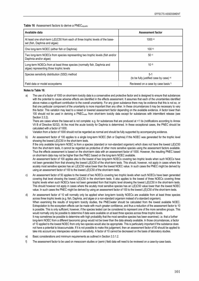
EFFECTS ASSESSMENT
101
Table 16 Assessment factors to derive a PNECaquatic
Available data Assessment factor
At least one short-term L(E)C50 from each of three trophic levels of the base-set (fish, Daphnia and algae)
1000 a)
One long-term NOEC (either fish or Daphnia) 100 b)
Two long-term NOECs from species representing two trophic levels (fish and/orDaphnia and/or algae)
50 c)
Long-term NOECs from at least three species (normally fish, Daphnia andalgae) representing three trophic levels
10 d)
Species sensitivity distribution (SSD) method 5-1 (to be fully justified case by case) e)
Field data or model ecosystems Reviewed on a case by case basis f)
Notes to Table 16:a) The use of a factor of 1000 on short-term toxicity data is a conservative and protective factor and is designed to ensure that substances
with the potential to cause adverse effects are identified in the effects assessment. It assumes that each of the uncertainties identifiedabove makes a significant contribution to the overall uncertainty. For any given substance there may be evidence that this is not so, orthat one particular component of the uncertainty is more important than any other. In these circumstances it may be necessary to varythis factor. This variation may lead to a raised or lowered assessment factor depending on the available evidence. A factor lower than100 should not be used in deriving a PNECwater from short-term toxicity data except for substances with intermittent release (seeSection 3.3.2).There are cases where the base-set is not complete: e.g. for substances that are produced at <1 t/a (notifications according to AnnexVII B of Directive 92/32). At the most the acute toxicity for Daphnia is determined. In these exceptional cases, the PNEC should becalculated with a factor of 1000.Variation from a factor of 1000 should not be regarded as normal and should be fully supported by accompanying evidence.
b) An assessment factor of 100 applies to a single long-term NOEC (fish or Daphnia) if this NOEC was generated for the trophic levelshowing the lowest L(E)C50 in the short-term tests.If the only available long-term NOEC is from a species (standard or non-standard organism) which does not have the lowest L(E)C50from the short-term tests, it cannot be regarded as protective of other more sensitive species using the assessment factors available.Thus the effects assessment is based on the short-term data with an assessment factor of 1000. However, the resulting PNEC basedon short-term data may not be higher than the PNEC based on the long-term NOEC available.An assessment factor of 100 applies also to the lowest of two long-term NOECs covering two trophic levels when such NOECs havenot been generated from that showing the lowest L(E)C50 of the short-term tests. This should, however, not apply in cases where theacutely most sensitive species has an L(E)C50 value lower than the lowest NOEC value. In such cases the PNEC might be derived byusing an assessment factor of 100 to the lowest L(E)C50 of the short-term tests.
c) An assessment factor of 50 applies to the lowest of two NOECs covering two trophic levels when such NOECs have been generatedcovering that level showing the lowest L(E)C50 in the short-term tests. It also applies to the lowest of three NOECs covering threetrophic levels when such NOECs have not been generated from that trophic level showing the lowest L(E)C50 in the short-term tests.This should however not apply in cases where the acutely most sensitive species has an L(E)C50 value lower than the lowest NOECvalue. In such cases the PNEC might be derived by using an assessment factor of 100 to the lowest L(E)C50 of the short-term tests.
d) An assessment factor of 10 will normally only be applied when long-term toxicity NOECs are available from at least three speciesacross three trophic levels (e.g. fish, Daphnia, and algae or a non-standard organism instead of a standard organism).When examining the results of long-term toxicity studies, the PNECwater should be calculated from the lowest available NOEC.Extrapolation to the ecosystem effects can be made with much greater confidence, and thus a reduction of the assessment factor to 10is possible. This is only sufficient, however, if the species tested can be considered to represent one of the more sensitive groups. Thiswould normally only be possible to determine if data were available on at least three species across three trophic levels.It may sometimes be possible to determine with high probability that the most sensitive species has been examined, i.e. that a furtherlong-term NOEC from a different taxonomic group would not be lower than the data already available. In those circumstances, a factorof 10 applied to the lowest NOEC from only two species would also be appropriate. This is particularly important if the substance doesnot have a potential to bioaccumulate. If it is not possible to make this judgement, then an assessment factor of 50 should be applied totake into account any interspecies variation in sensitivity. A factor of 10 cannot be decreased on the basis of laboratory studies.
e) Basic considerations and minimum requirements as outlined in Section 3.3.1.2.f) The assessment factor to be used on mesocosm studies or (semi-) field data will need to be reviewed on a case-by-case basis.

EFFECTS ASSESSMENT
102
For compounds with a high log Kow no short-term toxicity may be found. Also, even in long-term tests this may be the case or steady state may still not have been reached. In fish tests fornon-polar narcotics, the latter can be substantiated by the use of long-term QSARs (see Section3.2.1.2 and Chapter 4 on the Use of QSARs). Use of a higher assessment factor can beconsidered in such cases where steady state does not seem to have been reached.
A long-term test has to be carried out for substances showing no toxicity in short-term tests if thelog Kow > 3 (or BCF > 100) and if the PEClocal/regional is > 1/100th of the water solubility(see Section 4.6). The long-term toxicity test should normally be a Daphnia test to avoidunnecessary vertebrate testing. The NOEC from this test can then be used with an assessmentfactor of 100. If in addition to the required long-term test a NOEC is determined from an algaltest of the base-set, an assessment factor of 50 is applied.
3.3.1.2 Calculation of PNEC using statistical extrapolation techniques
The effect assessment performed with assessment factors can be supported by a statisticalextrapolation method if the database on Species Sensitivity Distributions (SSDs) is sufficient forits application. If a large data set from long-term tests for different taxonomic groups is available(OECD, 1992d), statistical extrapolation methods may be used to derive a PNEC. The mainunderlying assumptions of the statistical extrapolation methods are as follows (OECD, 1992d):
• the distribution of species sensitivities follows a theoretical distribution function;• the group of species tested in the laboratory is a random sample of this distribution.
In general, the methods work as follows: long-term toxicity data are log transformed and fittedaccording to the distribution function and a prescribed percentile of that distribution is used ascriterion. Several distribution functions have been proposed. The US EPA (1985) assumes a log-triangular function, Kooijman (1987) and Van Straalen and Denneman (1989) a log-logisticfunction, and Wagner and Løkke (1991) a log-normal function. Aldenberg and Slob (1993)refined the way to estimate the uncertainty of the 95th percentile by introducing confidencelevels.
The approach of statistical extrapolation is still under debate and needs further validation. Anadvantage of these methods is that they use the whole sensitivity distribution of species in anecosystem to derive a PNEC instead of taking always the lowest long-term NOEC. However,such methods could also be criticised. Among the most common drawbacks, the reasons putforward are: the lack of transparency by using this method compared to the standard approach,the question of representativity of the selected test species, the comparability of differentendpoints, the arbitrary choice of a specific percentile and a statistical confidence level etc.
In response to these concerns it has been seen as necessary to provide some guidance on whenand how to use such methods. What is proposed below has been discussed during an ExpertConsultation Workshop on Statistical Extrapolation Techniques for Environmental EffectsAssessments, in London on 17-18th January 2001 (EC, 2001). Although the primary objective ofthis workshop was focused on how statistical extrapolation techniques might be used to derivePNECs in the assessments of metals and their compounds, the general principles outlined hereshould be also applicable for other substances.
EFFECTS ASSESSMENT
103
Input data
The methods should be applied on all reliable available NOECs from chronic/long-term studies,preferably on full life-cycle or multi-generation studies. NOECs are derived according toprevious considerations (Table 15).
Which taxonomic groups
It is important to include all available information on the mode of action of the chemical, inorder to evaluate the need to include possible other (sensitive) taxonomic groups or excludepossible over-representation of certain taxonomic groups, realising that the mode of action maydiffer between short-term effects and long-term effects and between taxonomic groups. Theminimum species requirements when using the Species Sensitivity Distribution method are:
• fish (species frequently tested include salmonids, minnows, bluegill sunfish, channel catfish,etc.);
• a second family in the phylum Chordata (fish, amphibian, etc.);• a crustacean (e.g. cladoceran, copepod, ostracod, isopod, amphipod, crayfish etc.);• an insect (e.g. mayfly, dragonfly, damselfly, stonefly, caddisfly, mosquito, midge, etc.);• a family in a phylum other than Arthropoda or Chordata (e.g. Rotifera, Annelida, Mollusca,
etc.);• a family in any order of insect or any phylum not already represented; • algae;• higher plants.
It is recognised that for some of the taxa mentioned above, no internationally standardised testguidelines for long-term tests are currently available. The applicability of existing test data andthe fulfilment of the above requirements thus need to be assessed on a case-by-case basis. Thereis a need to evaluate additional information in order to assess how relevant and representative thelist of taxonomic groups is to the risk assessment scenario being investigated.
Minimal sample size (number of data)
Confidence can be associated with a PNEC derived by statistical extrapolation if the databasecontains at least 10 NOECs (preferably more than 15) for different species covering at least8 taxonomic groups.
Deviations from these recommendations can be made, on a case-by-case basis, throughconsideration of sensitive endpoints, sensitive species, mode of toxic action and/or knowledgefrom structure-activity considerations.
How to deal with multiple data for one species?
Where appropriate and possible, a pre-selection of the data should be performed in relation torealistic environmental parameters for Europe (e.g. hardness of water, pH, organic matter and/ortemperature). The full database should be carefully evaluated to extract information (e.g., onsensitive endpoints), which may be lost when “averaging” the data to a single value.
The test data applicable to the most sensitive endpoint should be taken as representative for thespecies. In this context, demographic parameters can be used as endpoints, as can bio-markers ifthey are toxicologically relevant in terms of population dynamics.

EFFECTS ASSESSMENT
104
Multiple values for the same endpoint with the same species should be investigated on a case-by-case basis, looking for reasons for differences between the results. For equivalent data on thesame end-point and species, the geometric mean should be used as the input value for thecalculation. If this is not possible, perhaps because valid results are considered to be too variable,then grouping and combining the values, e.g. by pH ranges, and using reduced numbers ofvalues should be considered. The effects that these different treatments have on the derived value(and on the resulting risk characterisation) should be investigated and discussed.
Where it is considered that the results are limited to certain conditions (e.g. not appropriate forlow pH conditions) then these limitations should be explained. The values derived from differenttreatments of the data may be useful to indicate sensitive regions.
Fit to a distribution
Different distributions like e.g. log-logistic, log-normal or others may be used (Aldenberg andJaworska, 2000, Aldenberg and Slob, 1993). The log-normal distribution is a pragmatic choicefrom the possible families of distributions because of the available description of itsmathematical properties (methods exist that allow for most in depth analyses of variousuncertainties).
The Anderson–Darling goodness of fit test can be used in addition to the Kolmogorov-Smirnov-test, as a criterion for the choice of a parametric distribution for comprehensive data sets,because it gives more weight to the tails of the distribution. A lack of fit may be caused by verydifferent factors. One common factor seems to be the inclusion of several NOECs for speciestested in a single laboratory, where the same test concentrations were used for all species. Thestatistical determination of the NOEC can lead to the same value being obtained for severalspecies, showing up as a vertical row of NOECs in the cumulative distribution plots. Anotherreason for lack of fit is a possible bimodality of the SSD, due to a specific mode of action of thetested substance towards only some taxonomic groups of species.
Whatever the fit to a distribution, results should be discussed in regards to the graphicalrepresentation of the species distribution and the different p values that were obtained with eachtest. Finally, any choice of a specific distribution function should be clearly explained.
If the data do not fit any distribution, the left tail of the distribution (the lowest effectconcentrations) should be analysed more carefully. If a subgroup of species can be identified asparticularly sensitive and if the number of data on this subgroup is sufficient, the distribution canbe fit to this subgroup. In case of lack of fit, the SSD method should not be used.
Estimated parameter
For pragmatic reasons it has been decided that the concentration corresponding with the point inthe SSD profile below which 5% of the species occur should be derived as an intermediate valuein the determination of a PNEC. A 50% confidence interval (c.i.) associated with thisconcentration should also be derived.

EFFECTS ASSESSMENT
105
Estimation of the PNEC
The PNEC is calculated as:
AFicSSDPNEC .).%50(%5
=(69)
AF is an appropriate assessment factor between 5 and 1, reflecting the further uncertaintiesidentified. Lowering the AF below 5 on the basis of increased confidence needs to be fullyjustified. The exact value of the AF must depend on an evaluation of the uncertainties around thederivation of the 5th percentile. As a minimum, the following points have to be considered whendetermining the size of the assessment factor:
• the overall quality of the database and the endpoints covered, e.g., if all the data aregenerated from “true” chronic studies (e.g., covering all sensitive life stages);
• the diversity and representativity of the taxonomic groups covered by the database, and theextent to which differences in the life forms, feeding strategies and trophic levels of theorganisms are represented;
• knowledge on presumed mode of action of the chemical (covering also long-term exposure);• statistical uncertainties around the 5th percentile estimate, e.g., reflected in the goodness of
fit or the size of confidence interval around the 5th percentile, and consideration of differentlevels of confidence (e.g. by a comparison between the 5% of the SSD (50%) with the 5% ofthe SSD (95%));
• comparisons between field and mesocosm studies, where available, and the 5th percentileand mesocosm/field studies to evaluate the laboratory to field extrapolation.
A full justification should be given for the method used to determine the PNEC.
Further recommendations
NOEC values below the 5% of the SSD need to be discussed in the risk assessment report. Forexample if all such NOECs are from one trophic level, then this could be an indication that aparticular sensitive group exists, implying that some of the underlying assumptions for applyingthe statistical extrapolation method may not be met;
The deterministic PNEC should be derived by applying the “standard” Assessment FactorApproach on the same database;
If mesocosm studies are available, they should also be evaluated and a PNEC derived followingthe TGD according to the standard method (deterministic approach).
The various estimates of PNEC should be compared and discussed and the final choice of aPNEC be based on this comparison.

EFFECTS ASSESSMENT
106
3.3.2 Effects assessment for substances with intermittent release
For substances subject to intermittent release (see Section 2.3.3.4 for the definition ofintermittent release), a single exposure event may be of only short duration. At least for dynamicsystems such as rivers, the likelihood of long-term effects arising from such exposure is low, theprincipal risk being that of short-term toxic effects. Thus, the risk assessment should be based ona no-effect-concentration for intermittent release. In extrapolating to such a PNECwater,intermittent, therefore, generally only short-term effects need to be considered. It is thereforeproposed that, to derive a PNECwater, intermittent for such situations, an assessment factor of100 be normally applied to the lowest L(E)C50 of at least three short-term tests from threetrophic levels. The assessment factor is designed to take account of the uncertainty that exists inextrapolating from the results of short-term laboratory toxicity tests to short-term effects that canbe anticipated in the ecosystems.
In undertaking such an extrapolation, due account is taken of the biological variables of intra-and inter-species toxicity, as well as the general uncertainties in predicting ecosystem effectsfrom laboratory data. This extrapolation should be carried out with care. Some substances maybe taken up rapidly by aquatic organisms and this can lead to delayed effects even after exposurehas ceased. This will generally be taken into account by the assessment factor of 100 but theremay be occasions when a higher or lower factor would be appropriate. For substances with apotential to bioaccumulate the lowered assessment factor of 100 may not always be sufficient toprovide adequate protection. For substances with a known non-specific mode of action, inter-species variations may be low. In such cases, a lower factor may be appropriate. In no caseshould a factor lower than 10 be applied to a short-term L(E)C50 value.
3.4 EFFECTS ASSESSMENT FOR MICROORGANISMS IN SEWAGETREATMENT PLANTS (STP)
Since chemicals may cause adverse effects on microbial activity in STPs it is necessary to derivea PNECmicroorganisms (see Section 2.3.7). The PNECmicroorganisms will be used for the calculation ofthe PEC/PNEC ratio concerning microbial activity in STPs. Current test systems for measuringthe effect of chemicals on microbial activity have different endpoints and different levels ofsensitivity. A number of internationally accepted test systems exist (cf. table below). Availabledata (e.g. UBA, 1993; Reynolds et al., 1987) suggest the following order of increasingsensitivities among particular test systems: respiration inhibition test (EU Annex V C.11; OECD209, 1984f) < inhibition control in base-set tests < growth inhibition test with P. putida <inhibition of nitrification.
In general, short-term measurements in the order of hours (e.g. 10 h) are preferred, in accordancewith the retention time in a STP. Information available on the toxicity for microorganisms hasalso to be relevant for the endpoint considered, i.e. microbial degradation activity in a STP. Testsystems such as the respiration inhibition test and the nitrification inhibition test can be used.Respiration tests using a mixed inoculum are considered more relevant than respirationinhibition tests using a single-species inoculum.
The assumption that the substance under investigation is not inhibitory to the microorganismswhen dosed in the test system is implicit in ready biodegradability testing (i.e., EU Annex VC.4A-F, OECD 301A-F, 1992f). Reynolds et al. (1987) report that microbial EC50 valuesdetermined for test substances using a variety of tests (Annex V C.11, OECD 209, 1984f, AnnexV C.4F, Closed Bottle Test, Growth Inhibition) were found to be inhibitory in ready

EFFECTS ASSESSMENT
107
biodegradability tests (Annex V C.4C,F,E,B; OECD 301B,C,D,E, 1992f). No-effect or EC0values were 1.5 to 10 times lower than the corresponding EC50 values. The authors recommendas a provisional rule that biodegradation testing should therefore be conducted at one-tenth of theEC50 concentration to ensure that a “probable non-inhibitory level” is employed inbiodegradation testing. It would, therefore, seem appropriate to consider the test concentrationfrom a positive ready biodegradability test to be an acceptable alternative to a NOEC obtainedfrom a microbial toxicity test for the purposes of determining a PNECmicroorganisms. This isparticularly the case if domestic sludge is used as the source of microorganisms and if there is noindication of toxicity for the test concentration, e.g. due to other available test results. Similarly,data from inherent biodegradability testing may also prove useful. However, some additionalissues have to be considered:
Only Ready Biodegradability Tests (RBT) relying on continuous monitoring, i.e. the MITI I test(EU Annex V C.4F; OECD 301C, 1992f) and the Manometric Respirometry test (EU Annex VC.4D; OECD 301F, 1992f), are considered reliable for observing the effects of a chemical on theinoculum, i.e. activated sludge diluted by factors ranging from ca. 100 to 1000. In parallel to thetest itself, a toxicity control is run in extra bottles containing both the test chemical and areference chemical that is easily degraded in the system. If for that purpose sodium acetate isused, the toxic effect is most often manifest as a delayed mineralisation of the substance.However, even if the vast majority of microorganisms are initially killed in the test system, sucha delay may only be in the order of a few hours or days before rapid mineralisation of sodiumacetate takes place. If measurements are carried out only weekly, which is the case in mostRBT's, a delay in mineralisation of sodium acetate of only a few days may not be detected,leading erroneously to the conclusion that the test chemical is not inhibitory. Sodium benzoatemay provide an acceptable alternative to sodium acetate when an inhibitory control test (i.e. theofficial term, not 'toxicity test') is performed with an RBT method that is not based oncontinuous monitoring, because mineralisation of benzoate occurs at a much slower rate.
Subject to expert judgement, consideration of data from biodegradation/removal studies usingthe laboratory/pilot scale Activated Sludge Simulation, Continuous Activated Sludge or AerobicSewage Treatment Coupled-Units tests (OECD 303A, 2001b; ISO-11733) may also prove usefulin any consideration of PNECmicroorganisms. These tests are laboratory scale models for simulationof activated sludge, representing realistic approximation to actual conditions within full scaleSTPs. A NOEC from well-conducted simulation studies using domestic activated sludge wouldcorrespond to the concentration of the chemical substance that does not perturb the properfunctioning of the Continuous Activated Sludge unit with regard to performance parameters suchas:
• test substance elimination;• COD removal;• nitrification;• denitrification;• phosphorus removal; • effluent quality etc.
when compared to a parallel non-dosed control.
Additionally, the results from tests with ciliated protozoa can be used for deriving aPNECmicroorganisms. In this case protozoa have to be regarded as additional species, not as anadditional trophic layer. Ciliated protozoa, constituting the most important class of protozoa inSTPs, are, except for certain industrial plants, important for their functioning. The toxicity data

EFFECTS ASSESSMENT
108
for ciliates are considered to be supplementary to the data for activated sludge or specificbacteria, i.e. no correlation exists between activated sludge and ciliate test results, neither areciliates consistently more sensitive. The data from one ciliate species are representative for otherciliates, i.e. test data from species not dominant or not present in STPs can serve as basis for thePNEC-derivation. The function of the protozoa in STP is correlated to their growth. Therefore,values from ciliate growth inhibition tests, preferably with Tetrahymena (cf. OECD, 1998a), arerelevant for the risk assessment for STPs. Tests using other characteristics (e.g. ciliary motion,cell movement, etc.) should not serve as a basis for the PNEC-derivation.
Often information may also be present on individual bacterial species such as from tests withVibrio fischeri (used in the MICROTOX test), Pseudomonas putida, Pseudomonas fluorescensand even Escherichia coli. These tests must be considered as less relevant. The tests with P.fluorescence and E. coli (Bringmann and Kühn, 1960) cannot be used for determination of thePNECmicroorganisms as they use glucose as a substrate. Likewise, the MICROTOX test cannot beused as it uses a saltwater species. Results of the cell multiplication inhibition test with P. putida(Bringmann and Kühn, 1980) should only be used for calculation of the PNECmicroorganisms incases where no other test results employing mixed inocula are available.
In general, the aim of the assessment is the protection of the degradation and nitrificationfunctions and process performance and efficiency of domestic and industrial STPs – as alsoinfluenced by protozoan populations. The toxicity of a substance to microorganisms in a STP isassessed by comparing the concentration of a substance in STP aeration tank with the microbialeffect concentration data for that substance (see also Section 2.3.7.1). If the substance underconsideration is relevant for industrial and municipal STPs the toxicity assessment should beconducted for both kinds of STPs separately. A PNECmicroorganisms should be obtained as a firststep in the effects assessment for microorganisms in both domestic and industrial sewagetreatment plants. The PNECmicroorganisms is usually derived from results obtained in the mostsensitive test system available, regardless of whether this is a test with activated sludge, relevantbacteria or ciliated protozoa:
• the PNECmicroorganisms is set equal to a NOEC from a test performed with ‘specific bacterialpopulations’ like nitrifying bacteria or P. putida or from a growth inhibition test performedwith ciliated protozoa. An EC50 from this test is divided by an assessment factor of 10;
• a NOEC or EC10 from other test systems like the respiration inhibition test (EU Annex VC.11; OECD 209, 1984f) is divided by an assessment factor of 10. An EC50 from this test isdivided by an assessment factor of 100;
• the lowest value is selected as the PNECmicroorganisms.
There may be cases in which the lowest PNECmicroorganisms does not correspond to the effect valueof the most sensitive test system because different AF (100 or 10) are applied to the different testsystems. In these cases expert judgement should be used to decide which effect value isappropriate for the calculation of the PNECmicroorganisms. Usually the effect value of the mostsensitive test system should be used as a basis for the calculation of PNECmicroorganisms employingthe appropriate AF.
Table 17 provides a complete listing of the test systems mentioned above, effect concentrationsthat are determined using them and the corresponding assessment factors.

EFFECTS ASSESSMENT
109
Table 17 Test systems for derivation of PNECmicroorganisms
Test Available value Assessment factor
Respiration inhibition tests NOEC or EC10 10
EU Annex V C.11; OECD 209 (1984f)ISO 8192 (1986)
EC50 100
Inhibition control in standardised biodegradation tests
- Ready biodegradability tests EU Annex V C.4 A-F; OECD 301A-F (1992f) 92/69/EEC C4 (1992) ISO-7827 (1994), -9439 (1999), -10707 (1994), -9408 (1999)
- Inherent biodegradability tests EU Annex V C.9; OECD 302 B-C (1981d-1992g) 88/302/EEC (1988) ISO-9888 (1999)
The tested concentration at which toxicityto the inoculum can be ruled out withsufficient reliability (cf. corresponding textsection above) could be considered as aNOEC for the toxicity to microorganisms ofa STP
10
Inhibition of nitrification NOEC or EC10 1
ISO-9509 (1989) EC50 10
Ciliate growth inhibition tests NOEC or EC10 1
(preferably with Tetrahymena, cf. OECD, 1998a) 1) EC50 10
Activated sludge growth inhibition tests NOEC or EC10 10
ISO-15522 EC50 100
Pilot scale activated sludge simulation tests
OECD 303A (2001b)ISO-11733
Based on case-by-case expert judgement,the tested concentration not impairingproper functioning of the CAS 2) unit couldbe considered as NOEC formicroorganisms in STPs
Case-by-casedown to
1
Growth inhibition test with Pseudomonas putida NOEC or EC10 1
NF EN ISO 10712 (1995) EC50 10
(Bringmann and Kühn, 1980) to be used if no other tests are available
Pseudomonas fluorescens(Bringmann and Kühn, 1960)
Not usable as it uses glucose as substrate
Escherichia coli(Bringmann and Kühn, 1960)
Not usable as it uses glucose as substrate
Vibrio fischeri (MICROTOX)NF EN ISO 11348-1, -2, -3 (1999)
Not relevant for STP as the bacterium is a saltwater species
Notes to Table 17:1) Ciliate testing would be required as the guideline becomes available2) CAS: Continuous Activated Sludge
EFFECTS ASSESSMENT
110
If on the basis of the PNECmicroorganisms derived using the procedures described above thePEC/PNEC ratio for industrial / domestic sewage treatment plants is above 1, the followingprocedure is proposed for refining the PNECmicroorganisms:
• If on the basis of a test with nitrifying bacteria, a PEC/PNEC ratio above 1 is derived for aspecific industrial STP, a revised PNECmicroorganisms for this specific site can be derived froma nitrification inhibition test using sludge from this site's STP. The revised PNECmicroorganismsfor a specific industrial STP is derived from this test using the assessment factors describedfor nitrifying bacteria. For domestic STPs a revision of the PNEC is not possible in this way- sludge from one STP can not be regarded as being representative (in comparison with thesingle species test) of all domestic STPs with respect to the nitrifying activity;
• If on the basis of a respiration inhibition test, a PEC/PNEC ratio above 1 is derived for aspecific industrial STP, a revised PNECmicroorganisms for this specific STP can be derived froma respiration inhibition test using sludge from this site's STP (the result from such a test issometimes already available). A revised PNECmicroorganisms for a specific industrial STP isderived from these tests using the assessment factors described above for respirationinhibition tests. A PNECmicroorganisms for domestic STPs can not be derived on the basis ofresults from respiration tests that use industrial sludge as the source of inoculum;
• If on the basis of a respiration inhibition test, a standardised biodegradation test or anactivated sludge growth inhibition or simulation test, a PEC/PNEC ratio above 1 is derivedfor a specific industrial sewage treatment plant, a revised PNECmicroorganisms for this site canbe derived from an appropriate pilot scale simulation test using activated sludge from thesite's STP as a source of inoculum;
• If on the basis of a single species test with ciliated protozoa a PEC/PNEC ratio above 1 isderived for municipal or industrial sewage treatment plants, a test reflecting the integrity ofthe native ciliate population in (industrial or domestic) sewage sludge is necessary. Theexception to this is where it can be shown that for the industrial STP under considerationprotozoa are not relevant. The ability of the protozoan community to eliminate externalbacterial food supply should be considered as a possible endpoint in this test. At present astandard protocol for a test based on ciliated protozoa which can be used to provide data forrevising a PNECmicroorganisms is not available.
3.5 EFFECTS ASSESSMENT FOR THE SEDIMENT
3.5.1 Introduction
Sediments may act as both a sink for chemicals through sorption of contaminants to particulatematter, and a source of chemicals through resuspension. Sediments integrate the effects ofsurface water contamination over time and space, and may thus present a hazard to aquaticcommunities (both pelagic and benthic) which is not directly predictable from concentrations inthe water column. Effects on benthic organisms are of concern because they constitute animportant link in aquatic food chain and play an important role in the recycling of detritusmaterial. Due to the lack of standardised test methods on, e.g., the role of microorganisms inrecycling of detritus material and nutrients, further tests needs to be developed and to be addedfor guidance in future.
It is unlikely that data for sediment dwelling organisms will be available for new substances. Todate, only a few tests with sediment organisms have been conducted in Europe with existingsubstances. However, research is in progress in this field in various countries. The selection of
EFFECTS ASSESSMENT
111
representative organisms and the selection of standardised sediments are still being discussed.Various approaches (e.g. equilibrium partitioning, interstitial water quality, spiked sedimenttoxicity, tissue residue, derived sediment quality criteria and standards) are being developed toinvestigate the effects that chemicals have on sediment and sediment organisms (OECD, 1992b).Only whole-sediment tests using benthic organisms are suitable for a realistic risk assessment ofthe sediment compartment. It is only by using such tests that it is possible to adequately addressall routes of exposure. A PNECsed can be derived from these tests that can be compared with thepredicted concentration in the sediment (PECsed) (based on measured or estimated values). Testprocedures are described in ASTM (1990 a–e), ASTM (1991, 1993 & 1994) and Burton (1991 &1992). No finalised international guidelines for whole-sediment tests are available. However, adraft OECD guideline for a chironomid toxicity test using spiked sediment exists (OECD,2001e). In addition OECD has prepared a detailed review paper on aquatic ecotoxicity testsincluding sediment test methods (OECD, 1998a). Examples of sediment toxicity tests for whichprotocols are available are listed in Appendix VI.
Statistical extrapolation methods for calculation of PNEC for sediment organisms could be usedwhen sufficient data are available (cf. Section 3.3.1.2.). Further guidance needs to be developedin future.
3.5.2 Strategy for effects assessment for sediment organisms
Substances that are potentially capable of depositing on or sorbing to sediments to a significantextent have to be assessed for toxicity to sediment-dwelling organisms. In addition, marinesediment effects assessment is necessary for substances that are known to be persistent in marinewaters, and may accumulate in sediments over time. In general, substances with a Koc < 500 –1000 L/kg are not likely sorbed to sediment (SETAC, 1993). To avoid extensive testing ofchemicals a log Koc or log Kow of ≥ 3 can be used as a trigger value for sediment effectsassessment.
For most chemicals the number of toxicity data on sediment organisms will be limited. For theinitial risk assessment, normally no effect data from tests with sediment organisms will beavailable. Therefore, the equilibrium partitioning method is proposed as a screening approach tocompensate for this lack of toxicity data. Results from this screening can be used as a trigger fordetermining whether whole-sediment tests with benthic organisms should be conducted. Testswith benthic organisms using spiked sediment are likely to be necessary if, using the equilibriumpartitioning method, a PEC/PNEC ratio > 1 is derived. The test results will enable a morerealistic risk assessment of the sediment compartment to be carried out.
Three situations can be distinguished for deriving a PNECsed:
• when no toxicity test results are available for sediment organisms, the equilibriumpartitioning method is applied to identify a potential risk to sediment organisms. Thismethod is regarded as “screening approach” and is explained in Section 3.5.3;
• when only acute toxicity test results for benthic organisms are available (at least one) therisk assessment is performed both on the basis of the test result of the most sensitive speciesusing an assessment factor of 1000 and on the basis of the equilibrium partitioning method.The lowest PNECsed is then used for the risk characterisation;
• when long-term toxicity test data are available for benthic organisms the PNECsed iscalculated using assessment factors for long-term tests and this result should prevail in therisk assessment. This approach is explained in Section 3.5.4.

EFFECTS ASSESSMENT
112
If no measured data are available, either for the determination of a PECsed or for the calculationof a PNECsed, no quantitative risk characterisation for sediment can be performed. In this casethe assessment conducted for the aquatic compartment will also cover the sediment compartmentfor chemicals with a log Kow up to 5. For substances with a log Kow > 5, or with a correspondingadsorption or binding behaviour, the PEC/PNEC ratio for the aquatic compartment is increasedby a factor of 10. This factor is justified by the fact that the equilibrium partitioning methodconsiders only the exposure via the water phase. The additional factor of 10 on the PEC/PNECratio takes into account the possible additional uptake via sediment ingestion (see Section 3.5.3).It has to be borne in mind that even this factor may be insufficient to achieve an appropriatelevel of protection in case of, for example, ionisable substances.
Table 18 presents an overview of different data configurations and explains how to use them forthe risk characterisation for sediment.
Table 18 Requirements for performing a risk characterisation for sediment
Available measured data:PECsed
Available measured data:PNECsed
Risk characterisation
Cpore water none Cpore water
PNECwater
Cbulk none Cbulk RHOsusp
Ksusp-water PNECwater.1000
none PNECsed Ksusp-water PECwater .1000
PNECsed RHOsusp
Cpore water PNECsed Ksusp-water Cpore water.1000
PNECsed RHOsusp
Cbulk PNECsed Cbulk
PNECsed
where:Cpore water concentration in sediment pore water [mg.l-1]Cbulk concentration in whole sediment [mg.kgsed-1]Ksusp water suspended matter-water partitioning coefficient [m3.m-3] eq. (10)RHOsusp bulk density of suspended matter [kg.m-3] eq. (4)
3.5.3 Calculation of PNEC using the equilibrium method
In the absence of any ecotoxicological data for sediment-dwelling organisms, the PNECsed maybe provisionally calculated using the equilibrium partitioning method. This method uses thePNECwater for aquatic organisms and the sediment/water partitioning coefficient as inputs(OECD, 1992b; Di Toro et al., 1991).
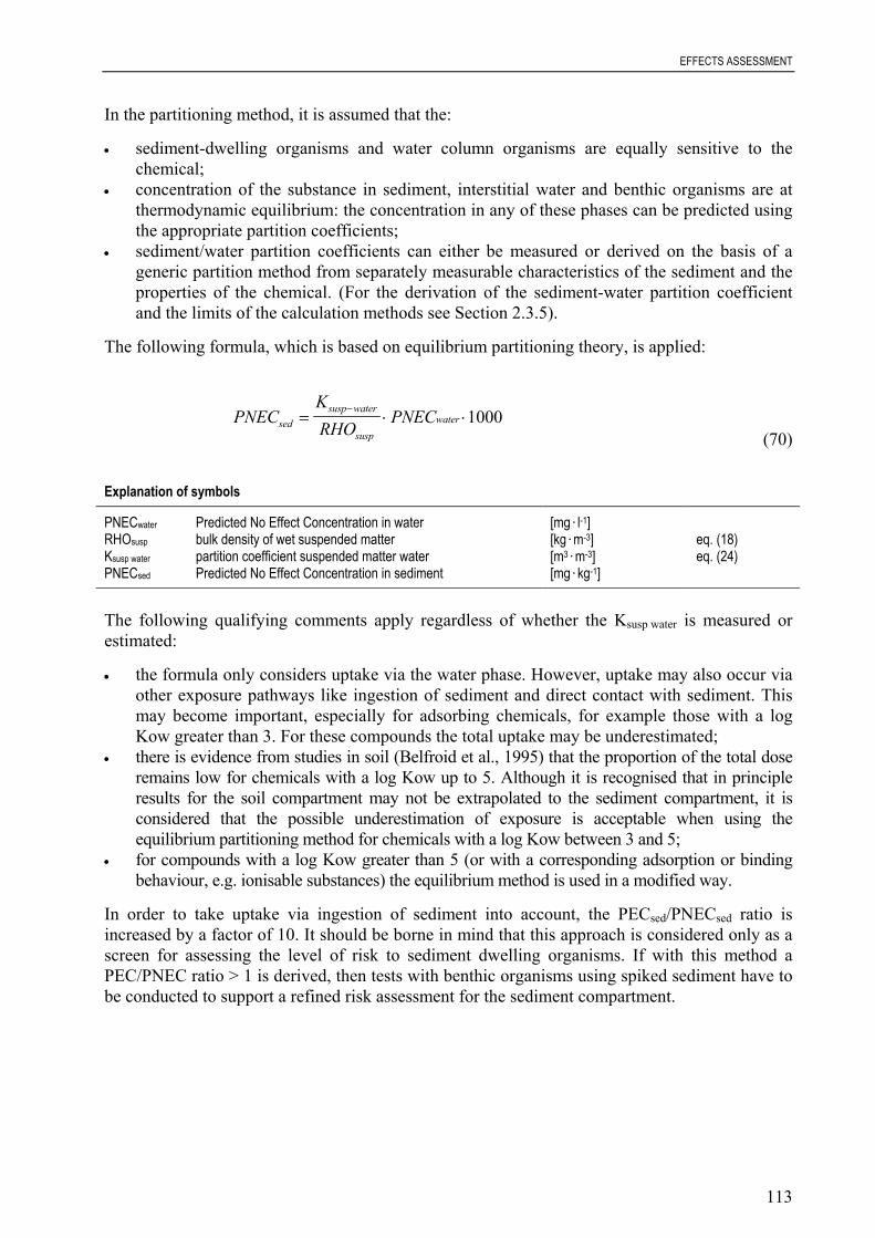
EFFECTS ASSESSMENT
113
In the partitioning method, it is assumed that the:
• sediment-dwelling organisms and water column organisms are equally sensitive to thechemical;
• concentration of the substance in sediment, interstitial water and benthic organisms are atthermodynamic equilibrium: the concentration in any of these phases can be predicted usingthe appropriate partition coefficients;
• sediment/water partition coefficients can either be measured or derived on the basis of ageneric partition method from separately measurable characteristics of the sediment and theproperties of the chemical. (For the derivation of the sediment-water partition coefficientand the limits of the calculation methods see Section 2.3.5).
The following formula, which is based on equilibrium partitioning theory, is applied:
PNECKRHO
PNECsedsusp water
suspwater= ⋅ ⋅− 1000
(70)
Explanation of symbols
PNECwater Predicted No Effect Concentration in water [mg.l-1]RHOsusp bulk density of wet suspended matter [kg.m-3] eq. (18)Ksusp water partition coefficient suspended matter water [m3.m-3] eq. (24)PNECsed Predicted No Effect Concentration in sediment [mg.kg-1]
The following qualifying comments apply regardless of whether the Ksusp water is measured orestimated:
• the formula only considers uptake via the water phase. However, uptake may also occur viaother exposure pathways like ingestion of sediment and direct contact with sediment. Thismay become important, especially for adsorbing chemicals, for example those with a logKow greater than 3. For these compounds the total uptake may be underestimated;
• there is evidence from studies in soil (Belfroid et al., 1995) that the proportion of the total doseremains low for chemicals with a log Kow up to 5. Although it is recognised that in principleresults for the soil compartment may not be extrapolated to the sediment compartment, it isconsidered that the possible underestimation of exposure is acceptable when using theequilibrium partitioning method for chemicals with a log Kow between 3 and 5;
• for compounds with a log Kow greater than 5 (or with a corresponding adsorption or bindingbehaviour, e.g. ionisable substances) the equilibrium method is used in a modified way.
In order to take uptake via ingestion of sediment into account, the PECsed/PNECsed ratio isincreased by a factor of 10. It should be borne in mind that this approach is considered only as ascreen for assessing the level of risk to sediment dwelling organisms. If with this method aPEC/PNEC ratio > 1 is derived, then tests with benthic organisms using spiked sediment have tobe conducted to support a refined risk assessment for the sediment compartment.

EFFECTS ASSESSMENT
114
3.5.4 Calculation of PNEC using assessment factors
If results from whole-sediment tests with benthic organisms are available the PNECsed has to bederived from these tests using assessment factors. However, the available sediment tests shouldbe carefully evaluated. Special attention should be given to the pathways through which the testorganisms are exposed to the chemical and the test protocol should carefully be checked,whether feeding with unspiked food has possibly reduced exposure via sediment ingestion. Forassessing the toxicity of spiked sediment it is necessary to address adequately all possible routesof exposure. Sediment organisms can be exposed via their body surfaces to substances insolution in the overlying water and in the pore water and to bound substances by direct contactor via ingestion of contaminated sediment particles. The route that is most important is stronglyinfluenced by species-specific feeding mechanisms and the behaviour of the organism in, or on,the sediment. Test design parameters can have a bearing on the route of uptake of a substance.
A number of uncertainties have to be addressed (cf. Chapter 3.3.1) in establishing the size of theassessment factors. In contrast to the principle adopted for the aquatic compartment, it is notnecessary to have 3 acute sediment tests for the assessment factor of 1000 to be applicable.Results from long-term tests with sub-lethal endpoints such as reproduction, growth, emergence,sediment avoidance and burrowing activity are regarded as most relevant due to the generallylong-term exposure of benthic organisms to sediment-bound substances. Consequently, if resultsfrom short-term tests with sediment-dwelling organisms are only available (at least one) anassessment factor of 1000 is applied to the lowest value. In addition, the PNECsed should also becalculated from the PNECwater using the equilibrium-partitioning method. A reduction in the sizeof the assessment factor should only be accepted if results form long-term tests with sediment-dwelling organisms are available.
The PNECsediment is derived from the lowest available NOEC/EC10 obtained in long-term testsby application of the following assessment factors (Table 19):
Table 19 Assessment factors for derivation of PNECsed
Available test result Assessment factor
One long-term test (NOEC or EC10) 100
Two long-term tests (NOEC or EC10) with species representing different living and feeding conditions 50
Three long-term tests (NOEC or EC10) with species representing different living and feeding conditions 10
3.6 EFFECTS ASSESSMENT FOR THE TERRESTRIALCOMPARTMENT
3.6.1 Introduction
Chemicals can reach the soil via several routes: application of sewage sludge in agriculture,direct application of chemicals and deposition from the atmosphere. Consequently the possibilityof adverse effects has to be assessed. The proposed strategy in this section is based on assessingthe effects of chemicals on soil organisms. At the moment no strategy is available to assesspossible effects on soil functions such as filtration, buffering capacity and metabolic capacity.

EFFECTS ASSESSMENT
115
As mentioned in the introduction, the substances discharged into the soil can not only affect thesoil organisms but also can influence soil functions. Substances that are hydrophilic and that arereadily eluted with the rainwater into the ground water as well as those that geo-accumulate andthose that are poorly degradable in soil should be considered with special care. If the substance isa biocide directly applied/emitted to soil, then the methodology referred in the Technical Notesfor Guidance in support of Directive 98/8 concerning the placing of biocidal products on themarket is recommended (http://ecb.jrc.it/biocides/).
The terrestrial ecosystem comprises of an above-ground community, a soil community and agroundwater community. In this section only effects on soil organisms exposed directly via porewater and/or soil are addressed. It is recognised that the strategy described here must thereforebe regarded as provisional. However, reference is made to the strategy for the air compartment(Section 3.7) and for bioaccumulation and secondary poisoning of birds and mammals(Section 3.8). It is currently not possible to carry out effect assessment for the groundwatercommunity because no toxicity data are available. However, ecotoxicity tests with groundwaterfauna and microflora have been proposed by Notenboom and Boessenkool (1992) and VanBeelen et al. (1990).
The strategy described below is based on several documents relating to terrestrial effectsassessment: OECD (1989), Stavola (1990), Samsøe-Petersen and Pedersen (1994), UBA (1993)and Römbke et al. (1993).
3.6.2 Strategy for effects assessment for soil organisms
Standardised methods exist for the soil compartment but toxicity tests with terrestrial organismsare not yet included in a base set. For new substances toxicity tests with plants and earthwormscan be requested at level 1. At level 2 there are, as yet, no specific additional requirements toexamine effects on soil organisms. For existing substances data will probably be scarce: for mostchemicals the data set will consist of results from short-term tests with for example earthwormsand plants. Long-term tests methods are available (e.g. springtails and earthworms) but resultsfrom these tests are seldom available for existing substances. For biocides, toxicity tests withterrestrial organisms may be required depending on product type and expected use.
The equilibrium partitioning method can be applied to aquatic data to identify a PNEC for soilorganisms. However, this method cannot replace toxicity data for soil organisms and should onlybe considered as a screen for identifying substances requiring further testing.
In common with the aquatic compartment, the objective of the assessment is to identifysubstances that present an immediate or delayed danger to the soil communities.
Soil is a complex and heterogeneous medium in which biological processes are occurring.Microorganisms play an important role in degradation processes and the mineralisation oforganic matter, allowing nutrients to be re-cycled in the ecosystem. Soil invertebrates arecontributing to the recycling of elements and play a significant part in creating and maintaining agood soil structure. Finally, plants are primary producers and provide food for all otherheterotrophic organisms. Consequently, the protection of the soil community requires protectionof all organisms playing a leading role in establishing and maintaining the structure and thefunctioning of the ecosystem. The use of results from tests that represent different and significantecological functions in the soil ecosystem is therefore suggested.
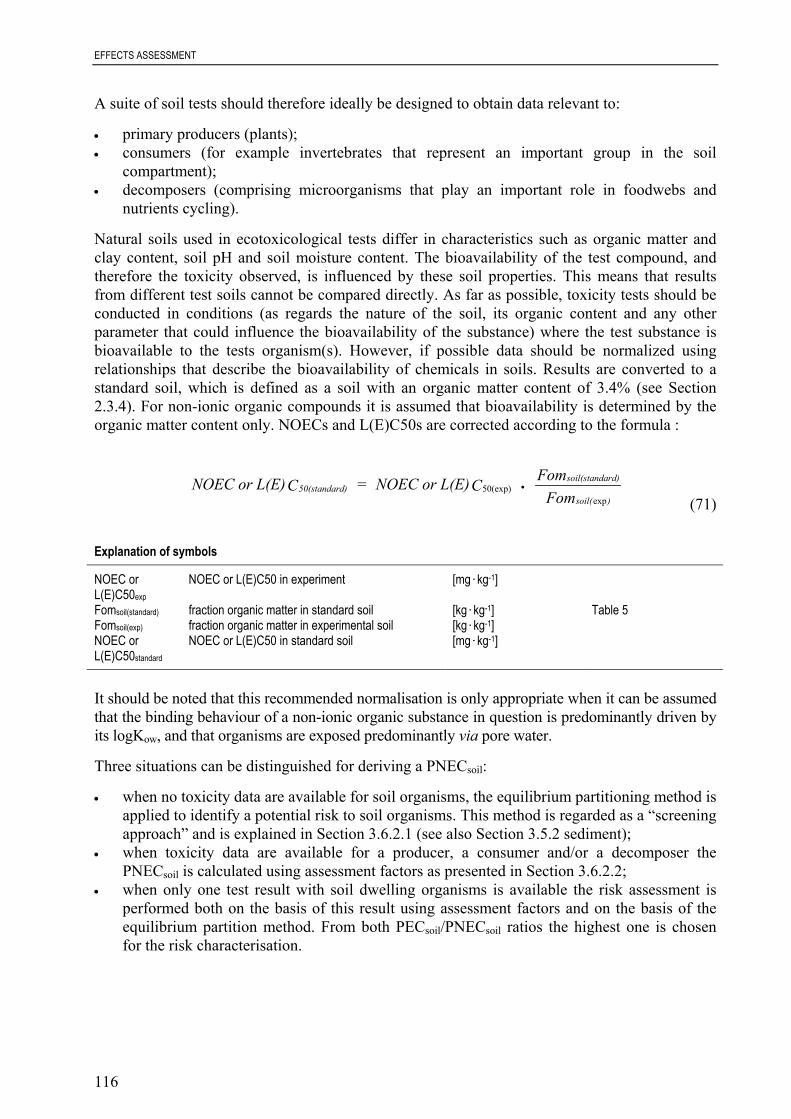
EFFECTS ASSESSMENT
116
A suite of soil tests should therefore ideally be designed to obtain data relevant to:
• primary producers (plants);• consumers (for example invertebrates that represent an important group in the soil
compartment);• decomposers (comprising microorganisms that play an important role in foodwebs and
nutrients cycling).
Natural soils used in ecotoxicological tests differ in characteristics such as organic matter andclay content, soil pH and soil moisture content. The bioavailability of the test compound, andtherefore the toxicity observed, is influenced by these soil properties. This means that resultsfrom different test soils cannot be compared directly. As far as possible, toxicity tests should beconducted in conditions (as regards the nature of the soil, its organic content and any otherparameter that could influence the bioavailability of the substance) where the test substance isbioavailable to the tests organism(s). However, if possible data should be normalized usingrelationships that describe the bioavailability of chemicals in soils. Results are converted to astandard soil, which is defined as a soil with an organic matter content of 3.4% (see Section2.3.4). For non-ionic organic compounds it is assumed that bioavailability is determined by theorganic matter content only. NOECs and L(E)C50s are corrected according to the formula :
NOEC or L(E)C = NOEC or L(E)C FomFom
50(standard)soil(standard)
soil( )50(exp)
exp•
(71)
Explanation of symbols
NOEC or NOEC or L(E)C50 in experiment [mg.kg-1]L(E)C50expFomsoil(standard) fraction organic matter in standard soil [kg.kg-1] Table 5Fomsoil(exp) fraction organic matter in experimental soil [kg.kg-1]NOEC or NOEC or L(E)C50 in standard soil [mg.kg-1]L(E)C50standard
It should be noted that this recommended normalisation is only appropriate when it can be assumedthat the binding behaviour of a non-ionic organic substance in question is predominantly driven byits logKow, and that organisms are exposed predominantly via pore water.
Three situations can be distinguished for deriving a PNECsoil:
• when no toxicity data are available for soil organisms, the equilibrium partitioning method isapplied to identify a potential risk to soil organisms. This method is regarded as a “screeningapproach” and is explained in Section 3.6.2.1 (see also Section 3.5.2 sediment);
• when toxicity data are available for a producer, a consumer and/or a decomposer thePNECsoil is calculated using assessment factors as presented in Section 3.6.2.2;
• when only one test result with soil dwelling organisms is available the risk assessment isperformed both on the basis of this result using assessment factors and on the basis of theequilibrium partition method. From both PECsoil/PNECsoil ratios the highest one is chosenfor the risk characterisation.

EFFECTS ASSESSMENT
117
3.6.2.1 Calculation of PNEC using the equilibrium partitioning method
The equilibrium partitioning method may not be suitable for lipophilic compounds or substanceswith a specific mode of action nor for species that are exposed primarily through food (VanGestel, 1992). Furthermore, this approach does not consider the effects on soil organisms ofchemicals that are adsorbed to soil particles and taken up by ingestion.
The PNECsoil is calculated as follows:
1000 PNEC RHOK =PNEC water
soilsoil
soil water
••
−
(72)
Explanation of symbols
PNECwater Predicted No Effect Concentration in water [mg.l-1]RHOsoil bulk density of wet soil [kg.m-3] eq. (18)Ksoil-water partition coefficient soil water [m3.m-3] eq. (24)PNECsoil Predicted No Effect Concentration in soil [mg.kg-1]
The applicability of the equilibrium partitioning method has been evaluated less for soil than forsediment-dwelling organisms. Van Gestel and Ma (1993) have shown the model to be valid forshort-term toxicity of several chlorophenols, chlorobenzenes and chloroanilines to earthworms.In order to take uptake by soil ingestion into account the same approach is used as for thederivation of the PNECsediment. Thus, the PECsoil/PNECsoil ratio is increased by a factor of 10 forcompounds with a log Kow > 5 (or for compounds with a corresponding adsorption or bindingbehaviour, e.g. ionisable substances).
In principle, toxicity data for aquatic organisms cannot replace data for soil dwelling organisms.This is because the effects on aquatic species can only be considered as effects on soil organismsthat are exposed exclusively to the soil pore water of the soil (Samsøe-Petersen and Pedersen,1994). Therefore, if the PECsoil/PNECsoil ratio that is calculated using the equilibriumpartitioning method is greater than 1, tests with soil organisms should be considered as anessential requirement for a refined effects assessment.
3.6.2.2 Calculation of PNEC using assessment factors
The same assessment factors used for the aquatic compartment (see Table 16) are applied to theterrestrial compartment (see Table 20). The size of the assessment factor therefore againdepends on the type of data that are available i.e. short-term or long-term toxicity test, thenumber of trophic levels tested and the general uncertainties in predicting ecosystem effectsfrom laboratory data. The assessment factors suggested for the soil compartment are not basedon comprehensive experience. As already stated information from tests with soil organisms willonly be available for some compounds. Furthermore, in most cases this information will be fromshort-term tests with earthworms. This means that a deeper understanding of the differencebetween short- and long-term toxicity for several taxonomic groups and the difference betweenlaboratory and field tests is needed. The choice of taxonomic groups for which toxicity data arenecessary (conform the base-set of algae, Daphnia and fish for the aquatic environment), is alsoa point of discussion. A dataset comprising of toxicity data for primary producers, consumersand decomposers is preferred. However, an internationally accepted set of standardised

EFFECTS ASSESSMENT
118
ecotoxicological tests for hazard assessment of chemicals for the soil compartment is notcurrently available.
Reference can be made to Section 6.3.4 and an OECD project in which a testing strategy forterrestrial ecosystems is being developed (Léon and Van Gestel, 1994). In summary, theassessment factors proposed in Table 20 must be regarded as indicative. As more information onthe sensitivity of soil organisms becomes available these factors may have to be revised.
Table 20 Assessment factors for derivation of PNECsoil
Information available Assessment factor
L(E)C50 short-term toxicity test(s) (e.g. plants, earthworms, or microorganisms) 1000
NOEC for one long-term toxicity test (e.g. plants) 100
NOEC for additional long-term toxicity tests of two trophic levels 50
NOEC for additional long-term toxicity tests for three species of three trophic levels 10
Species sensitivity distribution (SSD method) 5 – 1, to be fully justified on a case-by-casebasis (cf. main text)
Field data/data of model ecosystems case-by-case
A PNECsoil is calculated on the basis of the lowest determined effect concentration. If resultsfrom short-term tests with a producer, a consumer and/or a decomposer are available, the resultis divided by a factor of 1000 to calculate the PNECsoil. If only one terrestrial test result isavailable (earthworms or plants), the risk assessment should be performed both of this test resultand on the basis of the outcome of the aquatic toxicity data to provide an indication of the risk.As a matter of precaution, the larger PECsoil/PNECsoil ratio determines which further actionsshould be taken in the framework of the further testing strategy. If additional soil test results areavailable the assessment factors given in Table 20 should be applied.
3.6.2.3 Calculation of PNEC using statistical extrapolation techniques
Calculation of a PNECsoil using statistical extrapolation techniques can be considered whensufficient data are available (see Section 3.3.1.2. for minumum requirements). For comparabledata on the same end-point and species, by default the geometric mean should be used as theinput value for the calculation of the species sensitivity distribution. When results are availablefrom tests using different soils and it is likely that the soil characteristics have influence on theresults, the effect data should be normalised before further processing. If not possible, the lowestNOEC per end-point and species should be used. Data on microbial mediated processes andsingle species tests should be considered separately due to fundamental differences betweenthese tests (functional vs. structural test, multi-species vs. single species, adapted indigenousmicrobe community vs. laboratory test species, variability of test design and different endpoints,etc.). The results should be compared and evaluated on a case-by-case basis in deciding on afinal PNEC for the soil compartment.
The approach of statistical extrapolation is still under debate and needs further validation.
EFFECTS ASSESSMENT
119
3.7 EFFECTS ASSESSMENT FOR THE AIR COMPARTMENT
For the risk assessment of the air compartment biotic and abiotic effects are considered.
3.7.1 Biotic effects
The methodology used for effects assessment (and therefore the risk characterisation) ofchemicals in water and soil cannot be applied yet in the same manner to the atmosphere.Methods for the determination of effects of chemicals on species arising from atmosphericcontamination have not yet been fully developed, except for inhalation studies with mammals.
It is evident that the quantitative characterisation of risk by comparison of the PECair to PNECairis not possible at the moment: only a qualitative assessment for air is feasible.
For the air compartment toxicological data on animal species other than mammals are usuallynot or only scarcely available. For volatile compounds acute or short-term inhalation tests maybe present. On the basis of these data there may be indications of adverse effects. Short-termLC50 data can be used for a coarse estimation of the risk a chemical poses for animals.However, in most cases, it is unlikely that the atmospheric concentration of a chemical will behigh enough to cause short-term toxic effects in the environment, so data on long-term or chronictoxicity should be considered. For example, a chemical may be dangerous for the atmosphericenvironment at a low concentration, if it is classified as R 48 (“Danger of serious damage tohealth by prolonged exposure”). Also mutagenic effects and toxic effects on reproduction by achemical indicate a toxic potential for terrestrial vertebrates.
Fumigation tests on invertebrates are usually not available. For some existing substances andbiocides investigations on the toxicity to honey bees (Apis mellifera), which are conductedaccording to guidelines for the testing of plant protection agents, may be available. In these tests,it is sometimes difficult to determine the effective concentration and therefore a PNECair cannotbe derived.
Concerning the toxicity for plants, data from tests where a chemical is applied directly via air(gaseous or deposited) are normally scarce. When toxicity data are available or information isavailable that plants might be affected this information must be carefully screened and ifnecessary further plant toxicity testing can be requested. When no specific information ontoxicity to plants is available for the substance and considerable air emissions and exposure areexpected the information on related compounds (e.g. toxicity, phys.chem. properties) should bescreened and a decision should be made whether there is reason for concern and whether actualplant testing should be considered.
Some experience has been obtained over the last years on existing substances for which actualplant testing has been requested and performed (e.g. Risk assessment reports ontetrachloroethylene and dibutylphthalate, ECB, 2001). The test protocols have been developedon a case-by-case basis and varied from relatively simple laboratory test designs that can beconsidered as screening tests, to very extensive long-term open-top chambers with a largevariety of species. Further discussion is needed before these test designs can be standardised andinserted in a more rigid testing strategy for plants.
How the results of the available toxicity test should be used in the actual setting of a PNEC forplants has yet to be decided on a case-by-case basis. Like with the effects assessments for the

EFFECTS ASSESSMENT
120
other compartments it is expected that an assessment factor be applied to the available effectsdata. The selection of this factor should take into account factors such as:
• the type of tests that have been performed;• the duration of these tests; • the variety of species tested;• the type and severity of the effects observed.
3.7.2 Abiotic effects
For the evaluation of an atmospheric risk, the following abiotic effects of a chemical on theatmosphere have to be considered:
• global warming;• ozone depletion in the stratosphere;• ozone formation in the troposphere;• acidification.
If for a chemical there are indications that one or several of these effects occur, expertknowledge should be consulted. A first quantitative approach is described in De Leeuw (1993):
Global warming
The impact of a substance on global warming depends on its IR absorption characteristics and itsatmospheric lifetime. A potential greenhouse gas shows absorption bands in the so-calledatmospheric window (800-1,200 nm).
Stratospheric ozone
A substance may have an effect on stratospheric ozone if;
• the atmospheric lifetime is long enough to allow for transport to the stratosphere, and;• it contains one or more Cl, Br or F substituents.
In general, ozone depletion potential values approach zero for molecules with atmosphericlifetimes less than one year.
Tropospheric ozone
The generation of tropospheric ozone depends on a number of factors:
• the reactivity of the substance and the degradation pathway;• the meteorological conditions. The highest ozone concentrations are expected at high
temperatures, high levels of solar radiation and low wind speeds;• the concentration of other air pollutants. The concentration of nitrogen oxides has to exceed
several ppb.
Highly reactive compounds (e.g. xylene, olefins or aldehydes) contribute significantly to theozone peak values. Species with a low reactivity (e.g. CO, methane) are important for ozoneformation in the free troposphere and therefore for the long-term ozone concentrations.However, all studies showed significant variability in the tropospheric ozone building potentialvalues assigned to each organic component. It has to be concluded that at present there is no

EFFECTS ASSESSMENT
121
procedure available to estimate the effect on tropospheric ozone if only the basic characteristicsof a substance are known.
Acidification
During the oxidation of substances containing Cl, F, N or S substituents, acidifying components(e.g. HCl, HF, NO2 and HNO3, SO2 and H2SO4) may be formed. After deposition, theseoxidation products will lead to acidification of the receiving soil or surface water.
3.8 ASSESSMENT OF SECONDARY POISONING
3.8.1 Introduction
Bioconcentration and bioaccumulation may be of concern for lipophilic organic chemicals andsome metal compounds as both direct and indirect toxic effects may be observed upon long-termexposure. For metals guidance is given in Appendix VIII. Bioconcentration is defined as the netresult of the uptake, distribution and elimination of a substance in an organism due to water-borne exposure, whereas bioaccumulation includes all routes, i.e. air, water, soil and food.Biomagnification is defined as accumulation and transfer of chemicals via the food chain,resulting in an increase of the internal concentration in organisms at higher levels in the trophicchain. Secondary poisoning is concerned with toxic effects in the higher members of the foodchain, either living in the aquatic or terrestrial environment, which result from ingestion oforganisms from lower trophic levels that contain accumulated substances.
For many hydrophobic chemicals, accumulation through the food chain follows many differentpathways along different trophic levels. A good risk estimation of this complex process ishampered when only limited data from laboratory studies are available. One way to assess achemicals risk for bioaccumulation in aquatic species is to measure the Bioconcentration Factor(BCF). The static bioconcentration factor is the ratio between the concentration in the organismand the concentration in water in a steady-state (sometimes also called equilibrium) situation.When uptake and depuration kinetics are measured, the dynamic bioconcentration factor can becalculated from the quotient of the uptake and depuration rate constants:
fishfish
waterBCF = C
C or k
k1
2 (73)
Explanation of symbols
Cfish concentration in fish [mg.kg-1]Cwater concentration in water [mg.l-1]k1 uptake rate constant from water [l.kg-1.d-1]k2 elimination rate constant [d-1]BCFfish bioconcentration factor [l.kg-1]
For new and existing substances, the assessment of these processes is revised as moreinformation becomes available on toxicological and ecotoxicological effects and exposure. Atthe base-set level the available physico-chemical and (eco)toxicological information can be usedto decide whether or not there are indications for a potential for bioaccumulation and/or indirect

EFFECTS ASSESSMENT
122
effects. This estimation is used as a first step in the testing strategy for bioaccumulation andsecondary poisoning as will be explained in Section 3.8.3. For the terrestrial ecosystem a similarstrategy is used which is described in Section 3.8.3.7.
3.8.2 Indication of bioaccumulation potential
The simplest way to estimate the potential of a substance to bioaccumulate in aquatic species isby experimental measurement of the BCF. Determination of the BCF alone, however, only givesa partial picture of the potential of bioaccumulation, and additional data on uptake anddepuration kinetics, metabolism, organ specific accumulation and the level of bound residuesmay also be required. Such data will rarely be available and the potential for bioaccumulationwill usually need to be determined using simple physico-chemical and structural evidence(OECD, 2001c).
The most important and widely accepted indication of bioaccumulation potential is a high valueof the n-octanol/water partition coefficient. In addition, if a substance belongs to a class ofchemicals, which are known to accumulate in living organisms, it may have a potential tobioaccumulate. However, some properties of a substance may preclude high accumulation levelseven though the substance has a high log Kow or has a structural similarity to other substanceslikely to bioaccumulate. Alternatively there are properties, which may indicate a higherbioaccumulation potential than that suggested by a substance's low log Kow value. A survey ofthese factors is given below.
n-Octanol/water partition coefficient
At the base-set level, the potential for bioaccumulation can be estimated from the value of the n-octanol/water partition coefficient, log Kow. If this value cannot be determined experimentally,it may be calculated from the chemical structure.
It is accepted that values of log Kow greater than or equal to 3 indicate that the substance maybioaccumulate. For certain types of chemicals, e.g. surface-active agents and those which ionisein water, log Kow values may not be suitable for calculation of a BCF value. There are,however, a number of factors that are not taken into consideration when BCF is estimated onlyon the basis of log Kow values. These are:
• phenomena of active transport;• metabolism in organisms and the accumulation potential of any metabolites;• affinity due to specific interactions with tissue components;• special structural properties (e.g. amphiphilic substances or dissociating substances that may
lead to multiple equilibrium processes);• uptake and depuration kinetics (leading for instance to a remaining concentration plateau in
the organism after depuration).
n-Octanol only simulates the lipid fraction in organisms and therefore does not simulate otherpossibilities for storage and accumulation of substances and their metabolites in livingorganisms.
Adsorption
Adsorption onto biological surfaces, such as gills or skin, may also lead to bioaccumulation andan uptake via the food chain. Hence, high adsorptive properties may indicate a potential for both

EFFECTS ASSESSMENT
123
bioaccumulation and biomagnification. For certain chemicals, for which the octanol/waterpartition coefficient cannot be measured properly, a high adsorptive capacity (of whichlog Kp > 3 may be an indication) can be additional evidence of bioaccumulation potential.
Hydrolysis
The effect of hydrolysis may be a significant factor for substances discharged mainly to theaquatic environment: the concentration of a substance in water is reduced by hydrolysis so theextent of bioconcentration in aquatic organisms would also be reduced. Where the half-life, atenvironmentally relevant pH values (4-9) and temperature, is less than 12 hours, it can beassumed that the rate of hydrolysis is greater than that for uptake by the exposed organisms.Hence, the likelihood of bioaccumulation is greatly reduced. In these cases, it may sometimes beappropriate to perform a BCF test on the hydrolysis products, if identified, instead of the parentsubstance. However, it should be noted that, in most cases hydrolysis products are morehydrophilic and as a consequence will have a lower potential for bioaccumulation.
Degradation
Both biotic and abiotic degradation may lead to relatively low concentrations of a substance inthe aquatic environment and thus to low concentrations in aquatic organisms. However, theuptake rate may still be greater than the rate of the degradation processes, leading to high BCFvalues even for readily biodegradable substances. Therefore ready biodegradability does notpreclude a bioaccumulation potential, but for most substances concentrations will be low inaquatic organisms.
At the base-set level, only scarce information on the kinetics of degradation is available. For newsubstances even at higher tonnages, a request for such information would need to be justified; itcan be requested only on a case-by-case basis at level 2. For existing substances information ondegradation kinetics may be available.
If persistent metabolites are formed in substantial amounts the bioaccumulation potential of thesesubstances should also be assessed. However, for most substances information will be scarce.From experiments with mammals information may be obtained on the formation of possiblemetabolites, although extrapolation of results should be treated with care.
Molecular mass
Certain classes of substances with a molecular mass greater than 700 are not readily taken up byfish, because of possible steric hindrance at passage of gill membranes or cell membranes ofrespiratory organs. These substances are unlikely to bioaccumulate significantly (regardless ofthe log Kow-value).
Summary of indications of bioaccumulation potential
Taking the factors mentioned above into account will indicate whether or not there is potentialfor bioaccumulation. In summary: if, at base-set level, a substance:

EFFECTS ASSESSMENT
124
• has a log Kow ≥ 3; or;• is highly adsorptive; or;• belongs to a class of substances known to have a potential to accumulate in living
organisms; or;• there are indications from structural features;• and there is no mitigating property such as hydrolysis (half-life less than 12 hours);
there is an indication of bioaccumulation potential.
Reference is made to the OECD guidelines and to the guidance document on environmentalhazard classification (OECD, 2001c) in relation to interpretation of bioaccumulation studies andmeasurements of logKow. The test guidelines also contain information on the suitability of thevarious log Kow determination methods depending on the type of substance concerned.
3.8.3 Effects assessment for bioaccumulation and secondary poisoning
3.8.3.1 General approach
The assessment of the potential impact of substances on top predators is based on theaccumulation of hydrophobic chemicals through the food chains which may follow manydifferent pathways along different trophic levels. This accumulation may result in toxicconcentrations in predatory birds or mammals ingesting biota containing the chemical. Thiseffect is called secondary poisoning and should in principle be assessed by comparing themeasured or estimated concentrations in the tissues and organs of the top predators with the no-effect concentrations for these predators expressed as the internal dose. In practice, however,data on internal concentrations in wildlife animals are hardly ever available and most no-effectlevels are expressed in term of concentrations of the food that the organisms consume (i.e. inmg.kg-1 food). Therefore, the actual assessment (see below) is normally based on a comparisonof the (predicted) concentration in the food of the top predator and the (predicted) no-effectconcentration which is based on studies with laboratory animals. A distinction is made betweenthe methodology used to assess the effects of substances whose effects can be related directly tobioconcentration (direct uptake via water) and those where also indirect uptake via the food maycontribute significantly to the bioaccumulation. Bioaccumulation of metallic species is notconsidered explicitly in this section.
For substances with a log Kow < 4.5 the primary uptake route is direct uptake from the waterphase. In the absence of data on other uptake routes, it is assumed that the direct uptake accountsfor 100% of the intake. For substances with a log Kow ≥ 4.5, other uptake routes such as intakeof contaminated food or sediment may become increasingly important. Especially the uptakethrough the food chains eventually leading to secondary poisoning should be considered and astrategy for the assessment of secondary poisoning has been developed. This strategy takesaccount of the PECaquatic, the direct uptake and resulting concentration in food of aquaticorganisms and the mammalian and avian toxicity of the chemical. On this basis, possible effectsare estimated on birds and mammals in the environment via uptake through the food-chain water→ aquatic organisms → fish → fish-eating mammal or fish-eating bird (Romijn et al., 1993).Due to the lack of experience with this approach the assessment is considered as provisional.

EFFECTS ASSESSMENT
125
For some chemicals results from field measurements are available. Although interpretation isoften difficult, these results can be used to support the assessment of risks due to secondarypoisoning (Ma, 1994).
The first step in the assessment strategy is to consider whether there are indications forbioaccumulation potential. These indications have been discussed in the previous section.Subsequently, it is necessary to consider whether the substance has a potential to cause toxiceffects if accumulated in higher organisms. This assessment is based on classifications on thebasis of mammalian toxicity data, i.e. the classification Very Toxic (T+) or Toxic (T) or harmful(Xn) with at least one of the risk phrases R48 “Danger of serious damage to health by prolongedexposure”, R60 “May impair fertility”, R61 “May cause harm to the unborn child”, R62 “Possiblerisk of impaired fertility”, R63 “Possible risk of harm to the unborn child”, R64 “May cause harm tobreastfed babies”. Here it is assumed that the available mammalian toxicity data can give anindication on the possible risks of the chemical to higher organisms in the environment.
The current, either qualitative or quantitative, approach in the human health risk assessment forgenotoxic carcinogens is not practicable in the environmental part. Tumor incidence rates for agenotoxic carcinogen and subsequent cancer risks are related to individual risks in man and it isin most cases difficult to link those effects to populations. Endangoured species might be anexception, particularly those characterized by long-life-cycles where individuals may need to beprotected to support survival of the species. It is not unlikely, however, that the conservativeapproach followed in the risk assessment for man indirectly exposed via the environment forgenotoxic substances, will also be protective for individual top predators.
If a substance is classified accordingly or if there are other indications (e.g. endocrinedisruption), an assessment of secondary poisoning is performed.
A schematic view of the assessment scheme for the exposure route water → aquatic organisms→ fish → fish-eating mammal or fish-eating bird described above is given in Figure 14.
Figure 14. Assessment of secondary poisoning
No specific assessment of the risk to fish as a result of the combined intake of contaminants fromwater and contaminated food (aquatic organism) is considered necessary as this is assumed to becovered by the aquatic risk assessment and the risk assessment for secondary poisoning of fish-eating predators.
The risk to the fish-eating predators (mammals and/or birds) is calculated as the ratio betweenthe concentration in their food (PECoralpredator) and the no-effect-concentration for oral intake(PNECoral). The concentration in fish is a result of uptake from the aqueous phase and intake ofcontaminated food (aquatic organisms). Thus, PECoralpredator is calculated from thebioconcentration factor (BCF) and a biomagnification factor (BMF). Note that PECoralpredatorcould also be calculated for other relevant species that are part of the food of predators.
The details of the individual assessment steps are described in the following sections.
Water
Aquatic organism
FishPECoral,predator
fromBCF & BMF
Fish-eatingpredator

EFFECTS ASSESSMENT
126
3.8.3.2 Calculation of BCF from log Kow
If measured BCF values are not available, the BCF for fish can be predicted from therelationship between Kow and BCF. Various methods are available to calculate Kow. Often alarge variation is found in the Kow values of a chemical by using different methods. Thereforethe Kow-value must have been evaluated by an expert (see also Chapter 4 on the use of QSARs).For substances with a log Kow of 2-6 the following linear relationship can be used as developedby Veith et al. (1979).
log 0.85 log 0.70fish BCF = Kow • − (74)
Explanation of symbols
Kow octanol-water partition coefficient [-]BCFfish bioconcentration factor for fish on wet weight basis [l.kgwet fish]
For substances with a log Kow higher than 6 a parabolic equation can be used.
log .20 2.74 log 4.72fish2
BCF = logKow + Kow − −• •0 (75)
Explanation of symbols
Kow octanol-water partition coefficient [-]BCFfish bioconcentration factor for fish on wet weight basis [l.kgwet fish]
It should be noted that due to experimental difficulties in determining BCF values for suchsubstances this mathematical relationship has a higher degree of uncertainty than the linear one.Both relationships apply to compounds with a MW less than 700. For a discussion on bothrelationships see Chapter 4 (Use of QSARs).
3.8.3.3 Experimentally derived BCF
For existing substances an experimentally derived BCF may be present. For new substances aBCF test is mandatory at level 1. In most cases preference should be given to experimentallydetermined BCF values, especially if the test is conducted according to EU Annex V C.13 andOECD guideline 305 (OECD, 1996). The following parameters may be of importance whenconsidering the results of testing:
• BCF (bioconcentration factor);• CT50 (clearance time, elimination or depuration expressed as half-life);• metabolism/ transformation;• organ-specific accumulation (reversible/ irreversible);• incomplete elimination (bound residues);• substance bioavailability.
Recent work has shown that tests with substances with a high log Kow value result in highbioaccumulation factors if the chemical is carefully tested within the limit of its water solubility,

EFFECTS ASSESSMENT
127
i.e. without enhancement of solubility by the use of solubilisers. Also, the test duration is veryimportant because for highly hydrophobic chemicals it may take a very long time before a truesteady-state situation between water and organism has been reached. In addition, such lipophilicsubstances may be adsorbed onto biological surfaces such as gills, skin etc. which may lead totoxic effects in higher organisms after biomagnification.
For a more detailed guidance on interpretation of bioaccumulation test data, the OECD guidancedocument on environmental hazard classification (OECD, 2001c) may be consulted.
3.8.3.4 Calculation of a predicted environmental concentration in food
The concentration of contaminant in food (fish) of fish-eating predators (PECoralpredator) iscalculated from the PEC for surface water, the measured or estimated BCF for fish and thebiomagnification factor (BMF):
BMFBCFPECPEC fishwaterpredatororal ⋅⋅=, (76)
Explanation of symbols
PECoralpredator Predicted Environmental Concentration in food [mg.kgwet fish-1]PECwater Predicted Environmental Concentration in water [mg.l-1]BCFfish bioconcentration factor for fish on wet weight basis [l.kgwet fish-1]BMF biomagnification factor in fish [-]Table 21
The BMF is defined as the relative concentration in a predatory animal compared to theconcentration in its prey (BMF = Cpredator/Cprey). The concentrations used to derive and reportBMF values should, where possible, be lipid normalised.
An appropriate PECwater reflecting the foraging area of fish-eating mammals and birds should beused for the estimate. The foraging area will of course differ between different predators, whichmakes it difficult to decide on an appropriate scale. For example use of PEClocal may lead to anoverestimation of the risk as fish-eating birds or mammals do also forage on fish from other sitesthan the area around the point of discharge. Also, biodegradation in surface water is not takeninto account using PEClocal. However, using PECregional may have the opposite effect, as theremay be large areas in the 200.200 km region with higher concentrations. It has therefore beendecided that a scenario where 50% of the diet comes from a local area (represented by the annualaverage PEClocal) and 50% of the diet comes from a regional area (represented by the annualaverage PECregional) is the most appropriate for the assessment.
The biomagnification factor (BMF) should ideally be based on measured data. However, theavailability of such data is at present very limited and therefore, the default values given inTable 21 should be used. By establishing these factors it is assumed that a relationship existsbetween the BMF, the BCF and the log Kow (for further explanation, see Section 4.3.3 onmarine risk assessment). When measured BCF values are available, these should form the basisfor deciding on the size of the BMF.

EFFECTS ASSESSMENT
128
Table 21 Default BMF values for organic substances
log Kow of substance BCF (fish) BMF
<4.5 < 2,000 1
4.5 - <5 2,000-5,000 2
5 – 8 > 5,000 10
>8 – 9 2,000-5,000 3
>9 < 2,000 1
3.8.3.5 Calculation of the predicted no-effect concentration (PNECoral)
Only toxicity studies reporting on dietary and oral exposure are relevant as the pathway forsecondary poisoning is referring exclusively to the uptake through the food chain. Secondarypoisoning effects on bird and mammal populations rarely become manifest in short-term studies.Therefore, results from long-term studies are strongly preferred, such as NOECs for mortality,reproduction or growth. If no adequate toxicity data for mammals or birds are available, anassessment of secondary poisoning cannot be made.
For new substances, the results of mammalian repeated-dose toxicity tests are used to assesssecondary poisoning effects. For existing substances and biocides, toxicity data for birds (e.g.OECD test 205 (1984h) (LC50, 5-day acute avian dietary study) or OECD test 206 (1984i)(chronic)) may also be present. Extrapolation from such test results gives a predicted no-effectconcentration in food (PNECoral) that should be protective to other mammalian and avianspecies.
Acute lethal doses LD50 (rat, bird) are not acceptable for extrapolation to chronic toxicity, asthese are not dietary tests. Acute effect concentrations (e.g. OECD 205 (1984h)) for birds areacceptable for extrapolation. The results of the available mammalian or avian tests may beexpressed as a concentration in the food (mg.kgfood
-1) or a dose (mg.kg body weight.day-1)causing no effect. For the assessment of secondary poisoning, the results always have to beexpressed as the concentration in food. In case toxicity data are given as NOAEL only, theseNOAELs can be converted to NOECs with the following two formulae:
birdbirdbird CONVNOAELNOEC ⋅= (77)
mammalchroralmammalchrfoodmammal CONVNOAELNOEC ⋅= _,_, (78)
Explanation of symbols
NOECbird NOEC for birds (kg.kgfood–1) NOECmammal, food chr NOEC for mammals (kg.kgfood–1) NOAELbird NOAEL for birds (kg.kg bw.d-1) NOAELmammal, oral chr NOAEL for mammals (kg.kg bw.d-1) CONVbird conversion factor from NOAEL to NOEC (kg bw.d.kgfood –1) Table 22CONVmammal conversion factor from NOAEL to NOEC (kg bw.d.kgfood –1) Table 22

EFFECTS ASSESSMENT
129
Conversion factors for laboratory animals are presented in Table 22.
Table 22 Conversion factors from NOAEL to NOEC for several mammalian and one bird species
Species Conversion factor (bw/dfi)
Canis domesticus 40
Macaca sp. 20
Microtus spp. 8.3
Mus musculus 8.3
Oryctolagus cuniculus 33.3
Rattus norvegicus (> 6 weeks) 20
Rattus norvegicus (≤ 6 weeks) 10
Gallus domesticus 8
* bw = body weight (g); dfi: daily food intake (g/day)
NOECs converted from NOAELs have the same priority as direct NOECs.
The PNECoral is ultimately derived from the toxicity data (food basis) applying an assessmentfactor. In formula:
oral
oraloral AF
TOXPNEC = (79)
Explanation of symbols
PNECoral PNEC for secondary poisoning of birds and mammals [in kg.kgfood-1] AForal assessment factor applied in extrapolation of PNEC [-] Table 23TOXoral either LC50 bird, NOECbird or NOECmammal, food, chr [in kg.kgfood-1]
The assessment factor (AForal) takes into account interspecies variation, acute/subchronic tochronic extrapolation and laboratory data to field impact extrapolation. Some specificconsiderations need to be made for the use of the assessment factor for predators.
CCME (1998) contains wildlife data on body weight and daily food ingestion rates for 27 birdand 10 mammalian species. In addition, Schudoma et al. (1999) derived the mean body weightand daily food intake for the otter. The currently available set on wildlife bw/dfi ratios rangesfrom 1.1 to 9 for birds and from 3.9 to 10 for mammalian species. Comparison of these wildlifeconversion factors with the values given in Table 22 for laboratory species (8.3 – 40) shows thatthe wildlife species often have a lower bw/dfi ratio than laboratory animals. The difference canbe up to a factor 8 for birds and 10 for mammals. This difference is in theory accounted for in theuse of the interspecies variation factor that is part of the standard assessment factor. Theinterspecies variation, however, should comprise more than just the bw/dfi differences betweenspecies, e.g. the differences in intrinsic sensitivity. The protective value of the “normal”interspecies variation factor may therefore be questionable in case of predators. On top of that,many predator species are characterised by typical metabolic stages in their life-cycle that couldmake them extra sensitive to contaminants in comparison with laboratory animals (e.g.

EFFECTS ASSESSMENT
130
hibernation or migration). Similar to the bw/dfi differences, also this aspect goes beyond the“normal” interspecies variation.
The AForal should compensate for the above-mentioned specific aspects in the effectsassessment of predators. A factor of 30, accounting for both interspecies variation and lab-to-field extrapolation, is considered to be appropriate for this purpose. Aditionally,acute/subchronic to chronic extrapolation needs to be taken into account. The resultingassessment factors are given in Table 23.
Table 23 Assessment factors for extrapolation of mammalian and bird toxicity data
TOXoral Duration of test AForal
LC50 bird 5 days 3,000
NOECbird chronic 30
NOECmammal, food,chr 28 days90 dayschronic
3009030
If a NOEC for both birds and mammals is given, the lower of the resulting PNECs is used in therisk assessment.
3.8.3.6 Assessment of secondary poisoning via the aquatic food chain
It should be recognised that the schematic aquatic food chain water → aquatic organism → fish→ fish-eating bird or mammal is a very simplistic scenario as well as the assessment of risks forsecondary poisoning based on it. Any other information that may improve the input data or theassessment should therefore be considered as well. For substances where this assessment leads tothe conclusion that there is a risk of secondary poisoning, it may be considered to conductadditional laboratory tests (e.g. tests of bioaccumulation in fish or feeding studies withlaboratory mammals or birds) in order to obtain better data.
The simplified food chain is only one example of a secondary poisoning pathway. Safe levels forfish-eating animals do not exclude risks for other birds or mammals feeding on other aquaticorganisms (e.g. mussels and worms). Therefore it is emphasised that the proposed methodologygives only an indication that secondary poisoning is a critical process in the aquatic riskcharacterisation of a chemical.
For a more detailed analysis of secondary poisoning, several factors have to be taken intoaccount (US EPA, 1993; Jongbloed et al., 1994):
• differences in metabolic rates between animals in the laboratory and animals in the field;• normal versus extreme environmental conditions: differences in metabolic rate under normal
field conditions and more extreme ones, e.g. breeding period, migration, winter;• differences in caloric content of different types of food: cereals versus fish, worms or
mussels. As the caloric content of fish is lower than cereals birds or mammals in the fieldmust consume more fish compared to cereals for the same amount of energy needed leadingto a higher body burden of the pollutant;
• pollutant assimilation efficiency: differences in bioavailability in test animals (surfaceapplication of a test compound) and in the field (compound incorporated in food) and/or;
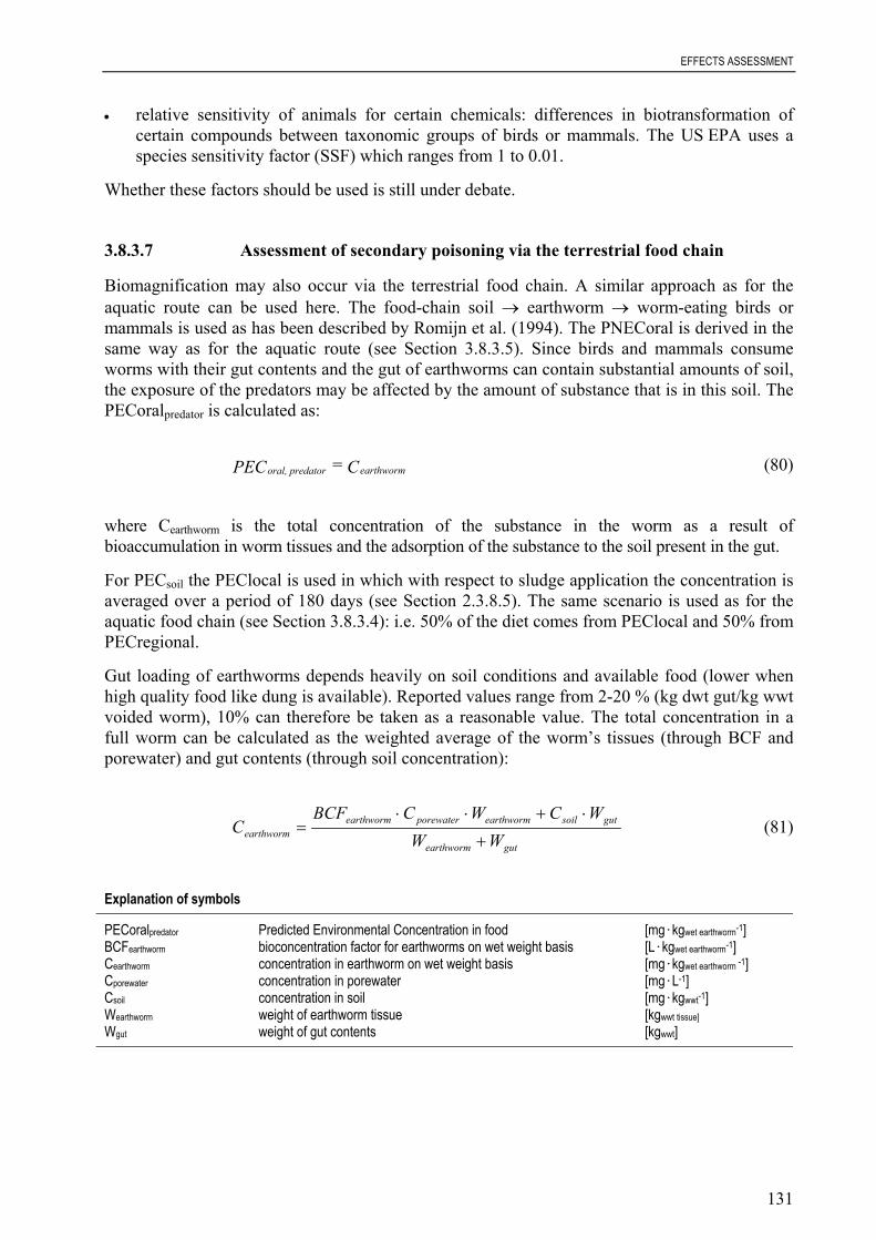
EFFECTS ASSESSMENT
131
• relative sensitivity of animals for certain chemicals: differences in biotransformation ofcertain compounds between taxonomic groups of birds or mammals. The US EPA uses aspecies sensitivity factor (SSF) which ranges from 1 to 0.01.
Whether these factors should be used is still under debate.
3.8.3.7 Assessment of secondary poisoning via the terrestrial food chain
Biomagnification may also occur via the terrestrial food chain. A similar approach as for theaquatic route can be used here. The food-chain soil → earthworm → worm-eating birds ormammals is used as has been described by Romijn et al. (1994). The PNECoral is derived in thesame way as for the aquatic route (see Section 3.8.3.5). Since birds and mammals consumeworms with their gut contents and the gut of earthworms can contain substantial amounts of soil,the exposure of the predators may be affected by the amount of substance that is in this soil. ThePECoralpredator is calculated as:
C =PEC earthwormpredator oral, (80)
where Cearthworm is the total concentration of the substance in the worm as a result ofbioaccumulation in worm tissues and the adsorption of the substance to the soil present in the gut.
For PECsoil the PEClocal is used in which with respect to sludge application the concentration isaveraged over a period of 180 days (see Section 2.3.8.5). The same scenario is used as for theaquatic food chain (see Section 3.8.3.4): i.e. 50% of the diet comes from PEClocal and 50% fromPECregional.
Gut loading of earthworms depends heavily on soil conditions and available food (lower whenhigh quality food like dung is available). Reported values range from 2-20 % (kg dwt gut/kg wwtvoided worm), 10% can therefore be taken as a reasonable value. The total concentration in afull worm can be calculated as the weighted average of the worm’s tissues (through BCF andporewater) and gut contents (through soil concentration):
gutearthworm
gutsoilearthwormporewaterearthwormearthworm WW
WCWCBCFC
+
⋅+⋅⋅= (81)
Explanation of symbols
PECoralpredator Predicted Environmental Concentration in food [mg.kgwet earthworm-1]BCFearthworm bioconcentration factor for earthworms on wet weight basis [L.kgwet earthworm-1]Cearthworm concentration in earthworm on wet weight basis [mg.kgwet earthworm -1] Cporewater concentration in porewater [mg.L-1]Csoil concentration in soil [mg.kgwwt-1]Wearthworm weight of earthworm tissue [kgwwt tissue]Wgut weight of gut contents [kgwwt]

EFFECTS ASSESSMENT
132
The weight of the gut contents can be rewritten using the fraction of gut contents in the total worm:
soilgutearthwormgut CONVFWW ⋅⋅= (82a)
where:
solidsolid
soilsoil RHOF
RHOCONV⋅
= (82b)
Explanation of symbolsCONVsoil conversion factor for soil concentration wet-dry weight soil [kgwwt.kgdwt-1] Fsolid volume fraction of solids in soil [m3.m-3] Table 5Fgut fraction of gut loading in worm kgdwt.kgwwt-1 0.1RHOsoil bulk density of wet soil [kgwwt.m-3] eq. (18)RHOsolid density of solid phase [kgdwt.m-3] Table 5
Using this equation, the concentration in a full worm can be written as:
soilgut
soilgutsoilporewaterearthwormearthworm CONVF
CONVFCCBCFC
⋅+
⋅⋅+⋅=
1(82c)
When measured data on bioconcentration in worms is available the BCF factors can be insertedin the above equation. For most substances, however, these data will not be present and BCF willhave to be estimated. For organic chemicals, the main route of uptake into earthworms will bevia the interstitial water. Bioconcentration can be described as a hydrophobic partitioningbetween the pore water and the phases inside the organism and can be modelled according to thefollowing equation as described by Jager (1998):
( ) earthwormowearthworm RHOKBCF 012.084.0 += (82d)
where for RHOearthworm by default a value of 1 (kgwwt.L-1) can be assumed.
Jager (1998) has demonstrated that this approach performed very well in describing uptake inexperiment with earthworms kept in water. For soil exposure, the scatter is larger and theexperimental BCFs are generally somewhat lower than the predictions by the model. The reasonsfor this discrepancy are unclear but may include experimental difficulties (a lack of equilibriumor purging method) or an underestimated sorption.4
4 According to certain studies some soil ingesting organisms may accumulate chemical substances not only from
the soil pore water but also directly (possibly by extraction in the digestive tract) from the fraction of thesubstance adsorbed onto soil particles. This may become important for strongly adsorbing chemicals, e.g. thosewith a logKow > 3. For these compounds the total uptake may be underestimated. In other studies however ithas been shown that soil digesters virtually only bioaccumulate the substance via the pore water, i.e.bioconcentrate chemical substances from the soil pore water. At present the latter process can be modelled byuse of the equilibrium partitioning theory (cf. also Section 3.5).

EFFECTS ASSESSMENT
133
Earthworms are also able to take up chemicals from food and it has been hypothesized that thisprocess may affect accumulation at log Kow>5 (Belfroid et al., 1995). The data collected byJager (1998), however, do not indicate that this exposure route actually leads to higher bodyresidues than expected on the basis of simple partitioning. Care must be taken in situationswhere the food of earthworms is specifically contaminated (e.g. in case of high concentrations inleaf litter) although reliable models to estimate this route are currently lacking.
The model was supported by data with neutral organic chemicals in soil within the range logKow 3-8 and in water-only experiments from 1-6. An application range of 1-8 is advised and it isreasonable to assume that extrapolation to lower Kow values is possible. The model could alsobe used for chlorophenols when the fraction in the neutral form was at least 5% and when bothsorption and BCF are derived from the Kow of the neutral species. The underlying data arehowever too limited to propose this approach in general for ionised chemicals.

MARINE RISK ASSESSMENT
134
4 ENVIRONMENTAL RISK ASSESSMENT – MARINE
4.1 INTRODUCTION
The extension of the existing risk assessment approaches to cover risks to the marineenvironment is a logical and important development in the establishment of a comprehensiverisk assessment methodology. Both the Commission report on the operation of several pieces oflegislation in the area of chemicals (COMMISSION, SEC (1998) 1986 final) as well as theOSPAR Hazardous Substances Strategy (OSPAR, 1998) recognise the need to extend the riskassessment framework and methodology as developed under Directive 93/67 and Regulation EC1488/94. This section, therefore, seeks to lay down the principles and concepts that should drivean assessment of the impacts on the marine environment. In doing so, it also identifies the areaswhere a similar approach can be adopted to that described elsewhere within the TGD, as well aselaborating different methodologies where they are considered more appropriate.
The assessment approaches detailed within the TGD have been developed principally to addressrisks, which might arise from emissions to the terrestrial and/or limnic aquatic environment.These schemes can and must nevertheless act as a starting point for the development of acomprehensive approach to risk assessment of substances in the marine environment, althoughdue recognition is given to the many differences both in technical detail and general approacheswhich may be necessary. It is not the intention of this section, therefore, to repeat technicaldescriptions or equations described elsewhere where the basic methodology for marineassessment do not differ significantly to that applied to the freshwater environment. Suchtechnical detail will be appropriately referenced to ensure that clarity is maintained. Rather, thesection will focus on new approaches, which are considered necessary to cover the uniquefeatures of the marine environment.
While the approaches to the assessment must conform to EC requirements for assessment underDirective 67/548, Regulation 793/93 and Directive 98/8, they must also recognise the objectivesestablished by OSPAR policy. The approaches will be guided and implemented, therefore, inaccordance with the EU policy under the above legislation as well as taking into account theOSPAR Strategy on Hazardous Substances. With respect to the OSPAR strategy the assessmentshould specifically contribute to the identification of the sources of release for a chemical andtheir relative significance in order to facilitate the eventual preparation of measures thatsubstantially, effectively and proportionately reduce the exposure.
The basic principles of the assessment have been derived in accordance with the experiencegathered by the procedure for chemicals in the frame of the original TGD (EC, 1996). Inattempting to extend current risk assessment methodology to cover the marine environment, it isnecessary to closely investigate the common concepts and protection goals of the availablemethods. Where common protection goals were identified, an examination of theappropriateness of the current methodologies to achieve them has been carried out.Modifications have been made where necessary to enhance relevance to the marine environment.Where environmental compartments were not adequately covered by the existing methodologies,new approaches have been elaborated based on a sound scientific understanding of the problemsand taking account, where appropriate, of the precautionary principle.
The approaches of the original TGD for the inland environment and that required for assessmentof the marine environment share a number of common principles and objectives. Each mustattempt to address the concern for the potential impact of individual substances on the

MARINE RISK ASSESSMENT
135
environment by examining both the exposures resulting from discharges/releases of chemicalsand the effects of such emissions on the structure and function of the ecosystem. In the TGD forthe inland environment this is practically done by considering five environmental compartments,namely the aquatic ecosystem, the terrestrial ecosystem, top predators, the functioning ofSewage Treatment Plants (STP) and the atmosphere. The environmental compartments areassessed at the local and the regional spatial scale by comparing the Predicted EnvironmentalConcentration (PEC) with the Predicted No Effect Concentration (PNEC) for the ecosystemusing data from representative species at different trophic levels for the particular environmentalcompartment. Top predators are assessed by assuming an exposure through the food chain. Theassessment addresses the functioning of the ecosystem as determined by the survival and well-being of all the species in the specific ecosystem. It is assumed that the protection of speciesprotects ecosystem structure and hence the ecosystem function. It addresses the survival andwell-being of species populations rather than an individual organism.
While this approach must clearly also apply to the marine environment, it must be recognisedthat the concepts and methodologies for the inland environment have largely been developedwith the local and regional spatial scales in mind, rather than the potential for global impact.There are, therefore, additional concerns for the risk assessment of the marine environment,which may not be adequately addressed by the methodologies used for the inland environmentalrisk assessment. These are:
a. the concern that hazardous substances may accumulate in parts of the marine environmentand that:(i) the effects of such accumulation are unpredictable in the long-term;(ii) that such accumulation would be practically difficult to reverse;
b. the concern that remote areas of the oceans should remain untouched by hazardoussubstances resulting from human activity, and that the intrinsic value of pristineenvironments should be protected.
Of these additional concerns (a) above may be seen as the main concern. This is characterised bya spatial and temporal scale not covered by the inland risk assessment approach. It is a concernthat chemical substances which can be shown both to persist for long periods and bioaccumulatein biota, can give rise to toxic effects after a greater time and at a greater distance than chemicalswithout these properties. While this is also true for the freshwater environment, the additionalconcern in the marine environment is that once the chemical has entered the open seas, anycessation of emission will not necessarily result in a reduction in chemical concentration andhence any effects become difficult to reverse. Equally, because of the long-term exposures andlong-life-cycle of many important marine species, effects may be difficult to detect at an earlystage.
To meet these concerns, which principally relate to substances that are considered as Persistent,Bioaccumulative and Toxic (referred to as PBTs), or have other properties which give rise to asimilar level of concern, an assessment approach will be detailed that will give specialconsideration to this new protection goal. In this context, the assessment of risk fulfilsspecifically the purpose of determining what are the sources, routes and pathways to the marineenvironment. This assessment will facilitate in the subsequent risk management decisions onwhich measures are the most effective in order to reduce the levels.
The structure of this section on marine risk assessment basically follows the structure of theinland environmental assessment. It starts with a section of exposure assessment where specificissues are highlighted relating to marine partitioning processes and marine degradation and

MARINE RISK ASSESSMENT
136
where a description is given on how the predicted environmental concentration (PEC) for thelocal and regional situation should be derived. In the next section on marine effects assessmentthe specific procedures for the derivation of predicted no-effect concentrations (PNECs) for theaquatic compartment and for sediment are described. This section also deals with the assessmentof possible effects through secondary poisoning via the foodchain in the marine environment.The section ends with the section on PBT assessment that describes criteria for identification ofpersistent, bioaccumulative and toxic substances and includes testing strategies to obtain thenecessary data for this identification. For the risk characterisation the reader is referred to Section 5.
4.2 MARINE EXPOSURE ASSESSMENT
4.2.1 Measured data
Guidance on the use of measured data in the environmental exposure assessment can be found inSection 2.2 of the TGD for the inland environment. This section covers the selection of adequatedata, the allocation of these data to the regional or local scale and deals with the questionwhether measured or estimated data (or both) should be used in the risk characterisation phase.
4.2.2 Partition coefficients
The distribution of a substance in the environment can be predicted from partition coefficients,which describe the relative concentrations between environmental compartments at equilibrium.Specific information on the derivation of the partitioning processes between air-aerosol, air-water, and solids-water in the various compartments can be found in Section 2.3.5. This sectiononly highlights some specific issues related to the marine environmental conditions.
Measured partition coefficients between water and a second compartment, if available, areusually derived from studies using non-saline water (freshwater or distilled/deionised water). Inthe absence of measured data, the relevant partition coefficients must be extrapolated from theprimary data listed in Section 2.3.2. However, the techniques that allow such an extrapolationare also largely based on freshwater data sets. Therefore, to assess the distribution of chemicalsin the marine environment, it is necessary to consider the extent to which partition coefficientsmay differ between seawater and freshwater.
The ionic strength, composition, and pH of seawater, compared with freshwater, have potentialeffects on the partitioning of a chemical with other compartments. To a large extent, these effectsare associated with differences in water solubility and/or speciation of the chemical, comparedwith freshwater. The relatively high levels of dissolved inorganic salts in seawater generallydecrease the solubility of a chemical (referred to as ‘salting-out’), by about 10-50% for non-polarorganic compounds but by a smaller fraction for more polar compounds (Schwarzenbach et al.,1993). A recent review found a typical reduction factor of 1.36 (Xie et al., 1997).
For non-ionisable organic substances, the decreased solubility in seawater, compared withfreshwater, is expected to result in proportional increases in the partition coefficients betweenwater and octanol, organic carbon and air. However, considering the uncertainty in measuredpartition values and the uncertainty associated with the frequent need to predict some or all ofthe partition coefficients, the differences attributable to the seawater environment (less than afactor of 2) are unlikely to be significant in risk assessment. Thus, unless measured seawater data
MARINE RISK ASSESSMENT
137
of equal reliability are available, freshwater data can be used for non-ionisable organiccompounds without adjustment for the marine environment.
For ionisable organic compounds, as for freshwater, the pH of the environment will affect thewater solubility and partitioning of the substance. There is some evidence that the degree ofdissociation may also be directly affected by the ionic strength of seawater (Esser and Moser,1982). However, the resulting shift in the dissociation curve is relatively small compared withthat which can occur due to pH for substances with dissociation constants close to the marinewater pH. It may, therefore, be preferable to obtain realistic measurements by use of seawaterinstead of deionised water. Another option is to measure the log Kow dependency of the pHdirectly (cf. the new draft OECD guideline 122 “Log Kow pH-metric method for ionisablesubstances” (OECD, 2000g). Because the pH of seawater (approximately 8) tends to be moreconstant than that of freshwater, the procedure to correct partition coefficients for ionisablesubstances, as described in Appendix XI, may however be considered sufficiently reliable formarine conditions.
For inorganic chemicals such as metals, the form or speciation of the substance can be directlyaffected by the ionic composition of seawater, which may have a considerable influence on bothsolubility and partitioning. On a case-by-case basis, there may be sufficient informationavailable to allow the relevant partition coefficient in seawater to be calculated from thefreshwater data; otherwise, measurements under marine conditions may be necessary.
4.2.3 Marine degradation
4.2.3.1 Abiotic degradation
Abiotic degradation (i.e. hydrolysis and photolysis) in marine environments should be assessedin a similar manner to abiotic degradation in freshwater environments except that the differentphysico-chemical conditions in marine environments should be taken into account. In particularthe stable pH of about 8 and the generally lower temperature of in average 9°C (282 K) shouldbe considered.
4.2.3.2 Biotic degradation
The rate of biodegradation in the various marine environments depends primarily on thepresence of competent degraders, the concentration and the intrinsic properties of the chemicalin question, the concentration of nutrients and organic matter and the presence of molecularoxygen. These factors vary significantly between various marine environments.
In estuarine environments, the supply of xenobiotics, nutrients and organic matter is much higherthan in more distant marine environments. These factors enhance the probability thatbiodegradation of xenobiotics occurs with a greater rate in estuaries than is the case in moredistant marine environments. Furthermore, estuarine and coastal environments are oftenturbulent and characterised by a constant sedimentation and re-suspension of sediment particlesincluding microorganisms and nutrients, which increase the biodegradation potential in theseenvironments compared to marine environments with a greater water depth. The presence ofsuspended particles and surfaces for attachment may favour the degradation of xenobiotics inestuarine environments.

MARINE RISK ASSESSMENT
138
ECETOC (1993) reviewed existing biodegradation data for the marine environments. Theyshowed that the biodegradation in estuaries was approximately a factor 4 lower than infreshwater environments for a variety of substances: Linear Alkylbenzene-Sulfonates, LinearAlkyl-Ethoxylates, m-cresol, chlorobenzenes, p-nitrophenol glutamate, hexadecane, andmethylparathion. However, for substances known to be very rapidly biodegradable (such assodium acetate, sodium benzoate and sodium dodecylsulphate), the rates were similar inestuarine and freshwater environments. In this section the average degradation potential inestuarine environments is assumed to be similar to the degradation potential in freshwaterenvironments.
Further away from the land-based sources of xenobiotics and allochthonous material theconditions for microorganisms are less favourable than close to land. The adaptation pressure islow due to much lower concentrations of xenobiotics as a result of degradation and dilution.Moreover, the environment can in general be characterised as oligotrophic, and theconcentrations of nutrients and organic matter are lower than in marine environments closer toland. Because of their low concentrations, the xenobiotics are hardly degraded as primarysubstrates, and due to the relatively low microbial activity the degradation of xenobiotics assecondary substrates is assumed to be limited. This implies that the degradation potential indistant marine environments is anticipated to be much lower than the degradation potential inestuaries.
A special case is areas with offshore-based sources as, e.g., oil platforms. It may be assumed thatthe microorganisms associated with the sediment may be more or less adapted to degradation ofchemicals that are continuously emitted from these sources. However, several factors, like e.g.nutrient limitation, may limit the biodegradation potential compared to the situation close toland. Furthermore, microorganisms in the water column will to a large extent drift with thecurrents and, therefore, a development of stable communities of competent degraders isimpeded.
Most marine sediments are anaerobic below the upper 0-5 mm. The assessment of thebiodegradation in marine sediments should ideally be based on results from investigationssimulating these conditions. If not available, other approaches may be used, e.g.:
• an approach similar to the one used for freshwater sediments could be used, i.e. to use ascenario consisting of a 30 mm thick sediment layer of which the upper 3 mm areconsidered aerobic and the remaining part anaerobic. If separate degradation rates areavailable for aerobic and anaerobic sediment, these could be used for estimating the half-life. If only data on aerobic degradation in sediment (or soil) is available, no degradation inthe anaerobic compartment should be assumed and consequently, a 10 times longer half-lifethan the half-life in aerobic sediment (or soil) should be used.
• anaerobic screening tests may be performed using a sediment inoculum (Horowitz et al.,1982; Madsen et al., 1995), and the observed biodegradability may then be used as anindication of the potential biodegradability of the substance in anaerobic sediment.Degradation rates should be derived by expert judgement.
• if no degradation data from studies with sediment or soil are available, the use of data ondegradation in water could be considered. The degradation potential in the upper aerobicsediment layer is generally assumed to be similar to the degradation potential in theoverlying water. However, the possible very low bioavailability in the sediment of highlyhydrophobic and/or poorly water-soluble substances should be taken into consideration as isdone also for freshwater sediments.

MARINE RISK ASSESSMENT
139
4.2.3.3 Marine biodegradation simulation tests
As a general rule, degradation rates or half-lives determined in tests simulating the conditions inthe actual aquatic environment should be considered for use whenever available. Expertjudgement of the validity and quality of the test data is necessary. The origin (e.g. relevance ofsampling site) of the seawater/sediment inoculum shall always be evaluated in connection withassessment and use of simulation test results. Biotransformation (identification of metabolisationpathways and major metabolites) and mineralisation data may be derived from one of thestandardised simulation tests by using samples from the particular environment as inoculum.Standardised simulation test methods for various marine compartments are:
• Aquatic (pelagic) compartment: ISO/DIS 14592-1 “Evaluation of the aerobicbiodegradability of organic compounds at low concentrations – Part 1” (draft method 2001)The ISO method has been the basis for a proposal for a new OECD guideline “Simulationtest - Aerobic transformation in surface water” (OECD, 2001d);
• Turbid aquatic/sediment dispersed compartment: ISO/DIS 14592-2 “Evaluation of theaerobic biodegradability of organic compounds at low concentrations – Part 2” (draftmethod, 2001b) and OECD 308: “Aerobic and anaerobic transformation in aquatic sedimentsystems” (aerobic test) (draft guideline, OECD, 2000c; draft Annex V C.24);
• Anaerobic sediment compartment: OECD 308 “Aerobic and anaerobic transformation inaquatic sediment systems” (strictly anaerobic test) (draft guideline, OECD, 2000c; draftAnnex V C.24). Data from anaerobic screening tests conducted with digested sewage sludge(e.g. ISO 11734, 1994) cannot be used for predicting the degradation potential in sediments.
4.2.3.4 Use of biodegradation screening test data
For most chemicals, however, no test data from such simulation tests are yet available. For manychemicals only data from screening tests are available. This may be data from marinebiodegradation screening tests or freshwater biodegradation screening tests. Marine screeningtests may be:
• the OECD 306 “Biodegradability in Seawater” test (OECD, 1992e) comprises two methods,the Shake Flask Method and the Closed Bottle Method. These tests are seawater variants ofthe Modified OECD Screening Test (EU Annex V C.4-B and OECD 301E, 1992f) andClosed Bottle Test (EU Annex V C.4-E and OECD 301D, 1992f), respectively, the maindifference being the use of a marine inoculum.
• three additional screening tests were subjected for a ring test initiated by the OSPARCommission in 1995-96. The tests are the “Marine CO2 Evolution Test”, the “MarineBODIS Test” and the “Marine CO2 Headspace Test”. The results of the ring test werereported by Elf & IARE (1996).
When only results from marine or freshwater biodegradation screening tests are available, it isrecommended to use the default mineralisation half-lives for the pelagic compartment asspecified in Table 24.
Table 24 Recommended mineralisation half-lives (days) for use in marine risk assessment when only screening test data areavailable
Freshwater 1) Estuaries 4) Other marineenvironments 5)
Degradable in marine screening test N.a. 15 50

MARINE RISK ASSESSMENT
140
Readily degradable 2) 15 15 50
Readily degradable, but failing 10-d window 50 50 150
Inherently degradable 3) 150 150 ∞
Persistent ∞ ∞ ∞
Notes to Table 24:1) Half-lives from Table 7.2) Pass level >70% DOC removal or > 60% ThOD in 28 days. Not applicable for freshwater.3) A half-life of 150 days may be used only for those inherently degradable substances that are quickly mineralised in the MITI II or the
Zahn Wellens Test (cf. TGD Chapter 2.3.6). The half-life of 150 days is not fully scientifically justifiable (cf. TGD Chapter 2.3.6), butreflects a “guesstimate consensus” between a number of experts.
4) Also including shallow marine water closest to the coastline5) The half-lives mentioned under this heading are normally to be used in the regional assessment (coastal model) as described in
Section 4.2.5.
The half-lives for the marine environments that are described in Table 24 are provisionalrecommendations, which should be reconsidered, when sufficient data for degradation ofdifferent substances in screening tests and simulation tests have been evaluated. The basis for therecommendation is the assumption that the degradation of xenobiotics in freshwater andestuarine waters in general can be described by similar degradation rates, whereas thedegradation rates are lower in other marine environments more distant from the coastline (Herethe half-life is suggested to be increased by a factor of three relative to estuaries for readilybiodegradable substances and even more for more slowly degradable substances, see Table 24).
4.2.4 Local Assessment
4.2.4.1 Introduction
Usually releases to the environment stem from a point source leading to a locally highenvironmental concentration of the substance. The highest risk resulting from discharges,emissions and losses of a chemical into the environment is expected to be at this local scale closeto the point of emission. It should be recognised that this might not always be the case and thatother local high concentrations can arise some distance from the point of an emission due tomarine currents, transport and deposition of sediments etc. Where this is considered possible fora local emission, specific modelling or measurements may be necessary. Since the aquaticconcentrations are highest at the point of emission, risks may be adequately assessed, at thislocal scale, using the existing methodologies.
MARINE RISK ASSESSMENT
141
In addition to the inland sources of emission, there may also be direct discharges to the marineenvironment. Thus, releases can occur from point sources:
• to estuaries, either by direct discharges or from inland sources via riverine inputs (or both);• to coastal areas;• to harbour areas from port activity and shipping;• to open sea e.g. from offshore oil and gas installations and from ships;• atmospheric deposition.
4.2.4.2 Calculation of PEClocal for the aquatic compartment
In the current procedure of inland environmental risk assessment, the use of marine exposurescenarios had become necessary whenever site-specific assessments were performed for a largenumber of industrial sites, of which some actually discharge directly to the sea. A riskassessment for the marine environment on a local scale was therefore only performed for specificsites identified as releasing directly into the sea. In the context of a dedicated methodology formarine risk assessment, a more generic exposure assessment for any given use is necessary.
While in some countries with long coastlines, the number of industrial sites dischargingwastewater to the sea is low compared with the overall number of sites (e.g. 5 – 10% in France;IFEN, 1997), it can be very high in others (e.g. 58 % in Sweden; SCB, 2000). It is thereforeassumed that for all uses of a given chemical substance, potential local releases to the marineenvironment can occur and, hence, it is necessary to perform a generic local exposure assessmentfor the local marine environment.
As for inland risk assessment, the calculation of the PEClocal depends mainly on twoparameters: dilution and the presence (or absence) of a STP. Both of these parameters have largeinfluences on the local concentration (Clocalseawater).
Regarding the presence or absence of a STP, conflicting information is available. Experiencewith the risk assessment of existing substances has shown that for chemical processing siteslocated on the coast, the probability that the effluents are treated in a biological treatment plant ismuch lower than for sites situated in land (see e.g., risk assessment reports for acrylonitrile,cyclohexane or methylene dianiline). This is confirmed by a survey performed by HELCOM(1998). While most industrial effluents from sites located on the Baltic Sea coast were treated(up to 98 %), the report did not contain detailed information on the treatment used from allcontracting parties of HELCOM. However, from the data compiled in Sweden it appears thatless than 50% of the industrial wastewater discharged passes a biological treatment step. On theother hand, statistics regarding treatment of municipal wastewater show that the treatment rate ofmunicipal wastewater from coastal municipalities is not different from overall treatment rates(e.g. IFEN, 1997; HELCOM, 1998). On the other hand, four EU Member States have appliedArticle 6 of Directive 91/271 allowing them to declare marine areas non sensitive to urbanwastewater meaning that they don’t have to treat the wastewater biologically but onlymechanically.
It is therefore proposed, for a default assessment, that in a local setting, industrial effluents(which may have been subject to some treatment on-site) are not treated in a municipalbiological STP. It is recognised though that the situation regarding the treatment of industrialeffluents is evolving rapidly and the present scenario could be revised in the near future. Whenthere is specific information available for a certain site that specific treatment facilities areavailable this information needs to be assessed and can be used to override the default

MARINE RISK ASSESSMENT
142
assumption. In practice this information is often available for production and/or large processingsites. It may also be possible to assume the presence of connection to an STP for certain industryand/or use categories if appropriate justification about the general connection frequency to theSTP for that specific industry is provided. For releases to municipal wastewater of substancesthat are used for private or public use (substances belonging to IC5 and IC6, Appendix I),however, it can be assumed that the degree of treatment in a biological STP corresponds to theinland scenario (see Section 2.3.7.1).
For discharges to a coastal zone, local dilution will be greater than in a freshwater river. First,initial dilution may occur if the density between the effluent and the saline receiving mediumdiffers (Lewis, 1997). The initial dilution factor is usually around 10. Further dilution due tocurrents can also be assumed, particularly if the point of release is subject to tidal influences. Inthe Baltic or the Mediterranean sea, where there are almost no tidal influences compared to theAtlantic Ocean or the North Sea, only initial dilution may occur on calm days, but normally,further dilution due to currents is probable. Dilution factors of more than 500 have beendetermined from model simulations (based on current measurements) in the North Sea, 200 maway from the discharge point (e.g. Pedersen et al., 1994).
A dilution factor for discharges to a coastal zone of 100 may then tentatively be assumed, whichseems to be representative of a realistic worst case. The same estimation method as for inlandexposure assessment can then be used to obtain the local concentration in seawater (Clocalseawater,see Section 2.3.8.3, equations 45-49).
In certain circumstances, it may be possible to identify specific emission points which wouldallow the use of more precise information regarding the available distribution and fate processes.Such “site-specific” assessments should only be used when it is known that all the emissionsemanating from the particular point in the life-cycle, e.g. manufacture, arise from a limitednumber of specific and identifiable points. In these circumstances each specific point of releasewill need to be assessed individually. If it is not possible to make this judgement, then the defaultassumptions should be applied. In “site-specific” assessments, due account can be taken of thetrue dilution available to the given emission as well as the impact of degradation, volatilisation,etc. in the derivation of the PEC. Normally, only dilution and adsorption to suspended sedimentneed be considered but site-specific conditions may indicate that valid local distribution modelscan be used.
For estuaries, which are influenced by currents and tidal movements, it is assumed as a firstapproach that they are covered by either the inland or the marine risk assessment. Thus, nospecific assessment is proposed.
Then, the local concentration in seawater can be obtained with:
DILUTION SUSP Kp + Clocal = Clocal
watersusp
effseawater
••• )101( 6-
(83)

MARINE RISK ASSESSMENT
143
Explanation of symbols
Clocaleff concentration of the substance in the STP effluent [mg.l-1] eq. (33)Kpsusp solids-water partitioning coefficient of suspended matter [l.kg-1] eq. (24)SUSPwater concentration of suspended matter in the seawater [mg.l-1] 15DILUTION dilution factor [-] 100Clocalseawater local concentration in seawater during emission episode [mg.l-1]
Kpsusp is derived as for inland risk assessment. For a specific estimation of the partitioningbehaviour of substances in saltwater environments see Section 4.2.2.
It is recognised that the dilution available to a discharge will also be related to the actual volumeof that discharge. In the freshwater scenario, this discharge volume is standardised to a volumeof 2,000 m3/day ie. the outflow from a standard STP. It is therefore proposed that the dischargevolume to the marine environment is also normalised at 2,000 m3/day such that the quantity ofthe substance discharged (in kg/day) is assumed, for modelling purposes, to be diluted into thisvolume prior to discharge.
For indirect human exposure and secondary poisoning, an annual average concentration insurface water is calculated:
365Temission Clocal = Clocal seawaterannseawater, •
(84)
Explanation of symbols
Clocalseawater local concentration in seawater during emission episode [mg.l-1] eq. (83)Temission number of days per year that the emission takes place [d.yr-1] App. IBClocalseawater,ann annual average local concentration in seawater [mg.l-1]
The concentration at the regional scale (PECregionalseawater) is used as background concentrationfor the local scale. Therefore, these concentrations are summed:
lPECregiona + Clocal = PEClocal seawaterseawaterseawater (85)
lPECregiona + Clocal = PEClocal seawaterannseawater,annseawater, (86)
Explanation of symbols
Clocalseawater local concentration in seawater during episode [mg.l-1] eq. (83)Clocalseawater,ann annual average concentration in seawater [mg.l-1] eq. (84)PECregionalseawater regional concentration in seawater [mg.l-1] 4.2.5PEClocalseawater predicted environmental concentration during episode [mg.l-1]PEClocalseawater,ann annual average predicted environmental concentration [mg.l-1]
If relevant site-specific information is available, it can be used to improve the assessment. Somesignificantly different exposure situations need to be reviewed though:

MARINE RISK ASSESSMENT
144
• substances released from offshore platforms. A harmonised mandatory control system forthe use and reduction of the discharge of offshore chemicals is already agreed withinOSPAR (OSPAR, 2000a;2000b). For this specific exposure situation within the EUlegislation, the methodology proposed by OSPAR can be taken into consideration5;
• substances released from harbours, marinas, fish farms and dry-docks. Specific scenarioswill have to be developed for these situations, which are most relevant for biocides.
4.2.4.3 Calculation of PEClocal for the sediment compartment.
The concentration in freshly deposited sediment is taken as the PEC for sediment; therefore theproperties of suspended matter are used. The concentration in bulk sediment can be derived fromthe corresponding water body concentration, assuming a thermo-dynamic partitioningequilibrium (Di Toro et al., 1991):
1000⋅⋅= −seawater
susp
watersuspsed PEClocal
RHOK
PEClocal(87)
Explanation of symbols
PEClocalseawater concentration in seawater during emission episode [mg.l-1]Ksusp-water suspended matter-water partitioning coefficient [m3.m-3] eq. (24)RHOsusp bulk density of suspended matter [kg.m-3] eq. (18)PEClocalsed predicted environmental concentration in sediment [mg.kg-1]
Highly adsorptive substances may not be considered adequately with the approach describedabove, as they are often not in equilibrium distribution between water and suspended matterbecause of their cohesion to suspended matter; however they may be desorbed after ingestion bybenthic organisms.
Suspended matter exposed to local releases can subsequently be transported over long distancesand deposited to sediment in distant areas. Therefore, it is possible that areas unrelated to localsettings are exposed to the same sediment concentrations as would be expected only in theimmediate vicinity of the releases. This has especially to be taken into account when comparingmeasured concentrations to estimated concentrations.
4.2.5 Regional assessment
For the release estimation of substances, a distinction is usually made between substances thatare emitted through point sources to which specific locations can be assigned, and substancesthat enter the environment through diffuse releases.
Point source releases may have a major impact on the environmental concentration on a localscale (PEClocal) and contribute to the environmental concentrations on a larger scale(PECregional). Like with the freshwater environment for the marine situation it is necessary to
5 The methodology for assessing releases from platforms (e.g. CHARM-model) that has been developed in the
context of these OSPAR decisions was not re-discussed in the context of the development of the presentguidance document for marine risk assessment.

MARINE RISK ASSESSMENT
145
evaluate the impact of substances that are released from point and diffuse sources over a widerarea. The PECregional is supposed to take into account the further distribution and fate of achemical upon release. The resulting PECregional is assumed to be a steady-state concentrationof the substance.
The regional system for the freshwater environment is a relatively large area of 200 by 200 kmwhich consists of 97% of soil and 3% of water. This system is surrounded by a larger area of thesize of Europe, called the continent (see Sections 2.1.2 and 2.3.8.7). If for the marine region anarea of similar size would be chosen where the water of the freshwater region would enter into,the resulting concentrations would be around 0.1% of the freshwater concentrations, mainly dueto the dilution of the freshwater in the much larger seawater region.
To assess the potential impacts of multiple point and diffuse sources of substances on the marineenvironment a river plume in coastal sea water is considered as a marine regional genericenvironment as follows:
An area of coastal sea that receives allthe water from the rivers from theregional system. This seawatercompartment is exchanging chemicalwith the continental seawatercompartment by dispersion andadvection (a current of seawaterflowing in a certain direction). Thesize of the coastal compartment is40 km long, 10 km wide and 10 mdeep. In addition to the input from theregional river water it receives 1% ofthe direct emissions from the inlandsources which is supposed torepresent a relevant fraction of thesources that are located near the seaand also have direct emissions intothe sea compartment. Most of therelevant characteristics of the coastalcompartment are similar to thefreshwater compartment apart fromthe suspended matter concentration that is set to 5 mg/l. In the absence of specific information(e.g. from marine simulation tests) it is assumed that the biodegradation rate in the water columnis approximately three times lower than in freshwater as described in Section 7.3. This scenariois shown in Figure 15.
This scenario can be modelled with the multi-media fate model that is used for the freshwaterPEC calculations, modified to allow dispersive exchange between the coastal zone to thecontinental sea water. By default, mixing of river water into the coastal sea gives a dilutionfactor of approximately 10. As a result concentrations in coastal seawater are expected to be afactor of 10 (for conservative chemicals) or more (for chemicals that react, volatilize orsediment) lower than in river water. The extent of degradation, volatilization, etc. in this coastalsea scenario is adequately modeled using the multi-media model.
continent
region
dispersion
advection cont . rivers
reg . rivers
exchange with global scales
Figure 15 Coastal sea scenario.
continent
region
dispersion
advection cont . rivers
reg . rivers
exchange with global scales
continent
region
dispersion
advection cont . rivers
reg . rivers
exchange with global scales

MARINE RISK ASSESSMENT
146
More details on the features of these models can be found in the section on calculation ofPECregional for the freshwater environment (Section 2.3.8.7.)6.
The calculation of PECregional according to this scenario provides the results for the genericrisk assessment that is necessary for the risk evaluation for new and existing substances andbiocides. Sufficient information on sources and emissions and site-specific information on thesuspended matter concentration, the flow rate and the dispersion velocity may be available so thegeneric assessment can be made more site-specific by overriding some of the default parametersor even can be replaced by site-specific models. The dispersion velocity greatly affects allcalculated concentrations, while in addition the suspended matter content further affects thedissolved concentration in seawater for chemicals with high log Kow. For the marineenvironment, models are available that can be used to assess the concentrations in certainspecific compartments (bays, estuaries, regions) of the marine environment to which specificindustrial sites discharge wastewater.
4.3 MARINE EFFECTS ASSESSMENT
4.3.1 Effects Assessment for the aquatic compartment
4.3.1.1 Introduction
Historically, the patterns of chemical production and usage resulting from urban and industrialdevelopment have led to the freshwater environment being considered to be the hydrospheremost at risk from these substances. Consequently, most regulatory schemes for evaluating thehazards and risks posed by new and existing substances have focussed primarily on theprotection of freshwater communities. As a result there is a considerable body of data on theecotoxicity of chemical substances to freshwater organisms (ECETOC, 1994a)7.
Where there is a need to assess the potential impact of substances entering estuarine and marinewaters, any hazard or risk assessment should ideally be based upon data generated using a rangeof ecologically relevant saltwater species (for example algae, invertebrates and fish). This isparticularly important given the greater diversity of species (particularly invertebrates) present in 6 A default length:width ratio of the coastal marine compartment has been set at 4:1. Assuming that this reflects the
plume shape in the generic assessment situation, this implies a ratio between the advective sea current along thecoast and the dispersive transport velocity perpendicular to that. If, in addition to the compartment dimensions, avalue is chosen for the sea current, the value of the lateral dispersion coefficient follows, or vice versa. If then avalue for the freshwater discharge into the coastal marine compartment is set too, mixing of freshwater withcoastal seawater is determined completely. In the generic regional model the river discharges approximately1000 m3/s into the continental model. With the dimensions of the sea compartment set to 40,000 m.10,000 m.10 m,and a suggested default value for the sea current of 0.03 m/s, taking into account the necessary dispersion coefficientof 50 m2/s, the freshwater content of the sea water inside the selected box would become approximately 10%.It should be noted that river water plumes in coastal waters vary greatly with local conditions (river flow, seacurrent, tide, depth, etc.). Prediction of site-specific dilution of river water into coastal seawater requires site-specific knowledge of flows and salinity distributions. Rhine and Meuse water (2,000 m3/s) are known to mix witha sea current of 0.035 m/s in the southern North Sea, yielding a very long-streched plume with approximately 20%river water in the first 10 km of the coast. A dispersion coefficient of 20 m2/s adequately describes this situation.The Amazon river is known for its great plume.
7 The ECETOC database consists of 2,203 entries on 361 chemicals, covering 121 species. Data on freshwaterspecies accounted for 1862 entries (84.5%) while data for saltwater (estuarine/marine) species accounted for341 entries (15.5%).

MARINE RISK ASSESSMENT
147
marine waters, relative to freshwaters (cf. Appendix XIV). There are also circumstances,however, where the special conditions existing in a particular environment such as that existingin the Baltic Sea, give rise to a reduced or limited species diversity and/or specific stresses suchas low or variable salinity. In such circumstances of low species diversity, adverse impacts inindividual species can have devastating impacts on the specialised ecosystem. Thus, while highspecies diversity may lead to a wide sensitivity distribution, but also considerable functionaloverlap, low species diversity may result in a lower sensitivity distribution but increase theecosystem function dependency on individual keystone species.
In both cases, the effects assessment must use, where possible, data relevant to theenvironmental compartment that is considered. However, compared to the situation forfreshwaters, there are relatively few data on the effects of chemical substances on estuarine andmarine organisms. Therefore, in practice there will be situations where saltwater toxicity data areneeded for hazard/risk assessments, but may not be available. In these situations it may benecessary to use freshwater data in lieu of data for estuarine/marine species (Schobben et al., 1994;Karman et al., 1998). In using data on freshwater species to characterise the risk in the marinewaters, a clear understanding of the comparability of effects data generated on both types of speciesis necessary. Furthermore, there is some evidence, e.g. for some metals, that species living inbrackish water are more susceptible because of the salinity (osmotic) stress they have to endure incontrast to those of the same species living in truly marine conditions. Under these circumstancesthe applicability of the toxicity data needs to be considered on a case-by-case basis.
4.3.1.2 Evaluation of data
It has been recognised for many years that there is a wider diversity of taxonomic groups(particularly invertebrates) in saltwaters compared to freshwaters and that many groups are onlyfound in marine waters (see Russell and Yonge, 1928; Tait, 1978). Moss (1988) stated that56 phyla were present in marine waters compared to 41 in freshwaters. No phyla are confined tofreshwaters only while 15 phyla are found only in marine waters. These differences are partlydue to the fact that multicellular animals originated in the seas and they have been wellpopulated since the earliest fossil records.
Nevertheless, an important part of any evaluation of data must involve an assessment of theusefulness of the main body of freshwater ecotoxicity data in predicting effects in the marineenvironment. Where such data can be used, the focus of further investigation can concentrate onadditional factors which specifically characterise the marine conditions. Studies conducted onthe comparability of sensitivity of freshwater and marine species have been hampered by the lowlevel of substances for which a comparable dataset has been available. Nevertheless where suchdata are available, it has tended to show that there is no systematic bias in sensitivity wherecomparable tests and endpoints are paired. A recent report which collated much of the availabledata confirmed these findings (ECETOC, 2000). Based on the currently available data, it can beconcluded that:
• overall, the data reviewed and current marine risk assessment practice suggest a reasonablecorrelation between the ecotoxicological responses of freshwater and saltwater biota - atleast for the usual aquatic taxa (i.e., fish, crustacea, algae). No marked difference insensitivity between freshwater and saltwater biota appears that systematically applies acrossall three trophic levels considered;
MARINE RISK ASSESSMENT
148
• where evaluated, differences between trophic levels within each medium were generally assignificant or even more marked than between media. Such variation is implicitly assumedin the use of assessment factors in current risk assessment practice;
• where differences in the apparent sensitivity of freshwater and marine biota were observedfor individual compounds, such differences were consistently within a factor of 10 (<1 logunit) and usually somewhat less;
• average differences in sensitivity for such paired species comparisons were typically withina factor of ~2;
• however, within trophic levels differences larger than a factor of 10 were shown for severalmetals and pesticides indicating that for these substances fresh water and saltwater datashould not be pooled for effects assessment and PNEC derivation.
The use of freshwater acute effects data in lieu of or in addition to saltwater effects data for riskassessment purposes is not contra-indicated by the empirical data reviewed. Use of pooled datais therefore recommended. Under such circumstances, PNEC values should be derived from themost sensitive endpoint regardless of the medium.
No comparison of long-term effects data has been made due to the lack of suitable data but againthere are no reasons to believe that a systematic bias to freshwater or marine species would exist.Therefore it is proposed that data on freshwater or marine fish, crustacea and algae be usedinterchangeably for evaluation of the risks to either compartment.
4.3.1.3 Derivation of PNEC
The greater species diversity in the marine environment, compared to freshwaters (seeAppendix XIV), including the presence of a number of taxa that occur only in that environment,may mean that the distribution of sensitivities of species is broader. It is necessary to consider,therefore, whether the three-taxa model offers sufficient certainty that sensitive species will becovered using the assessment factors developed for the freshwater systems. Since it is notpossible to make a clear judgement on the basis of available data, it is considered prudent toassume that this greater diversity of taxa will produce a broader distribution of speciessensitivity. Thus, where only data for freshwater or saltwater algae, crustaceans and fish isavailable a higher assessment factor than that for the derivation of PNECwater for freshwatersshould be applied, to reflect the greater uncertainty in the extrapolation. Where data is availablefor additional taxonomic groups, for example rotifers, echinoderms or molluscs the uncertaintiesin the extrapolation are reduced and the magnitude of the assessment factor applied to a datasetcan be lowered. Test protocols for these groups are available from organisations such as theAmerican Society for Testing and Materials, the International Council for the Exploration of theSeas and the United States Environmental Protection Agency (OECD, 1998a). The assessmentfactors given are based on current scientific understanding on the species comparability of toxicitybetween freshwater and saltwater species and the issue of differences in diversity in freshwatersand saltwaters. These may need to be revisited as additional information becomes available.
It is recognised that the assumption of a greater species sensitivity distribution covering theadditional marine taxa is based on limited data and is precautionary. The generation of additionaltoxicity data on marine species may allow this assumption to be further refined such that loweror higher assessment factors may be considered following a systematic review of accumulatingevidence.
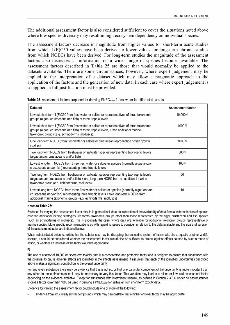
MARINE RISK ASSESSMENT
149
The additional assessment factor is also considered sufficient to cover the situations noted abovewhere low species diversity may result in high ecosystem dependency on individual species.
The assessment factors decrease in magnitude from higher values for short-term acute studiesfrom which L(E)C50 values have been derived to lower values for long-term chronic studiesfrom which NOECs have been derived. For long-term studies the magnitude of the assessmentfactors also decreases as information on a wider range of species becomes available. Theassessment factors described in Table 25 are those that would normally be applied to thedatasets available. There are some circumstances, however, where expert judgement may beapplied to the interpretation of a dataset which may allow a pragmatic approach to theapplication of the factors and the generation of new data. In each case where expert judgement isso applied, a full justification must be provided.
Table 25 Assessment factors proposed for deriving PNECwater for saltwater for different data sets
Data set Assessment factor
Lowest short-term L(E)C50 from freshwater or saltwater representatives of three taxonomicgroups (algae, crustaceans and fish) of three trophic levels
10,000 a)
Lowest short-term L(E)C50 from freshwater or saltwater representatives of three taxonomicgroups (algae, crustaceans and fish) of three trophic levels, + two additional marinetaxonomic groups (e.g. echinoderms, molluscs)
1000 b)
One long-term NOEC (from freshwater or saltwater crustacean reproduction or fish growthstudies)
1000 b)
Two long-term NOECs from freshwater or saltwater species representing two trophic levels(algae and/or crustaceans and/or fish)
500 c)
Lowest long-term NOECs from three freshwater or saltwater species (normally algae and/orcrustaceans and/or fish) representing three trophic levels
100 d)
Two long-term NOECs from freshwater or saltwater species representing two trophic levels(algae and/or crustaceans and/or fish) + one long-term NOEC from an additional marinetaxonomic group (e.g. echinoderms, molluscs)
50
Lowest long-term NOECs from three freshwater or saltwater species (normally algae and/orcrustaceans and/or fish) representing three trophic levels + two long-term NOECs fromadditional marine taxonomic groups (e.g. echinoderms, molluscs)
10
Notes to Table 25:Evidence for varying the assessment factor should in general include a consideration of the availability of data from a wider selection of speciescovering additional feeding strategies/ life forms/ taxonomic groups other than those represented by the algal, crustacean and fish species(such as echinoderms or molluscs). This is especially the case, where data are available for additional taxonomic groups representative ofmarine species. More specific recommendations as with regard to issues to consider in relation to the data available and the size and variationof the assessment factor are indicated below.When substantiated evidence exists that the substances may be disrupting the endocrine system of mammals, birds, aquatic or other wildlifespecies, it should be considered whether the assessment factor would also be sufficient to protect against effects caused by such a mode ofaction, or whether an increase of the factor would be appropriate.a)The use of a factor of 10,000 on short-term toxicity data is a conservative and protective factor and is designed to ensure that substances withthe potential to cause adverse effects are identified in the effects assessment. It assumes that each of the identified uncertainties describedabove makes a significant contribution to the overall uncertainty.For any given substance there may be evidence that this is not so, or that one particular component of the uncertainty is more important thanany other. In these circumstances it may be necessary to vary this factor. This variation may lead to a raised or lowered assessment factordepending on the evidence available. Except for substances with intermittent release, as defined in Section 2.3.3.4, under no circumstancesshould a factor lower than 1000 be used in deriving a PNECwater for saltwater from short-term toxicity data.Evidence for varying the assessment factor could include one or more of the following:− evidence from structurally similar compounds which may demonstrate that a higher or lower factor may be appropriate.

MARINE RISK ASSESSMENT
150
− knowledge of the mode of action as some substances by virtue of their structure may be known to act in a non-specific manner. A lowerfactor may therefore be considered. Equally a known specific mode of action may lead to a higher factor.
− the availability of data from a variety of species covering the taxonomic groups of the base set species across at least three trophiclevels. In such a case the assessment factors may only be lowered if multiple data points are available for the most sensitive taxonomicgroup (i.e. the group showing acute toxicity more than 10 times lower than for the other groups).
There are cases where a complete short-term dataset even for freshwater algal, crustacean and fish species will not be available, for examplefor substances which are produced at < 1 t/a (notifications according to Annex VII B of Directive 92/32). In these situations, the only data maybe short-term L(E)C50 data for Daphnia. In these exceptional cases, the PNEC should be calculated with a factor of 10,000.Variation from an assessment factor of 10000 should be fully reported with accompanying evidence.b)An assessment factor of 1000 applies where data from a wider selection of species are available covering additional taxonomic groups (suchas echinoderms or molluscs) other than those represented by algal, crustacean and fish species; if at least data are available for two additionaltaxonomic groups representative of marine species.An assessment factor of 1000 applies to a single long-term NOEC (freshwater or saltwater crustacean or fish) if this NOEC was generated forthe taxonomic group showing the lowest L(E)C50 in the short-term algal, crustacean or fish tests.If the only available long-term NOEC is from a species which does not have the lowest L(E)C50 in the short-term tests, it cannot be regardedas protective of other more sensitive species using the assessment factors available. Thus, the effects assessment is based on the short-termdata with an assessment factor of 10,000. However, normally the lowest PNEC should prevail. An assessment factor of 1000 applies also to the lowest of the two long-term NOECs covering two trophic levels (freshwater or saltwater algaeand/or crustacean and/or fish) when such NOECs have not been generated for the species showing the lowest L(E)C50 of the short-term tests.This should not apply in cases where the acutely most sensitive species has an L(E)C50-value lower than the lowest NOEC value. In suchcases the PNEC might be derived by applying an assessment factor of 1000 to the lowest L(E)C50 of the short-term tests. c)An assessment factor of 500 applies to the lowest of two NOECs covering two trophic levels (freshwater or saltwater algae and/or crustaceanand/or fish) when such NOECs have been generated covering those trophic levels showing the lowest L(E)C50 in the short-term tests withthese species. Consideration can be given to lowering this factor in the following circumstances:− It may sometimes be possible to determine with a high probability that the most sensitive species covering fish, crustacea and algae has
been examined, that is that a further longer-term NOEC from a third taxonomic group would not be lower than the data already available.In such circumstances an assessment factor of 100 would be justified;
− a reduced assessment factor (to 100 if only one short-term test, to 50 if two short-term tests on marine species are available) applied tothe lowest NOEC from only two species may be appropriate where:− short-term tests for additional species representing marine taxonomic groups (for example echinoderms or molluscs) have been
carried out and indicate that these are not the most sensitive group, and;− it has been determined with a high probability that long-term NOECs generated for these marine groups would not be lower than
that already obtained. This is particularly important if the substance does not have the potential to bioaccumulate.An assessment factor of 500 also applies to the lowest of three NOECs covering three trophic levels, when such NOECs have not beengenerated from the taxonomic group showing the lowest L(E)C50 in short-term tests. This should, however, not apply in the case where theacutely most sensitive species has an L(E)C50 value lower than the lowest NOEC value. In such cases the PNEC might be derived byapplying an assessment factor of 1000 to the lowest L(E)C50 in the short-term tests.d)An assessment factor of 100 will be applied when longer-term toxicity NOECs are available from three freshwater or saltwater species (algae,crustaceans and fish) across three trophic levels.The assessment factor may be reduced to a minimum of 10 in the following situations:− where short-term tests for additional species representing marine taxonomic groups (for example echinoderms or molluscs) have been
carried out and indicate that these are not the most sensitive group, and it has been determined with a high probability that long-termNOECs generated for these species would not be lower than that already obtained;
− where short-term tests for additional taxonomic groups (for example echinoderms or molluscs) have indicated that one of these is themost sensitive group acutely and a long-term test has been carried out for that species. This will only apply when it has been determinedwith a high probability that additional NOECs generated from other taxa will not be lower than the NOECs already available.
A factor of 10 cannot be decreased on the basis of laboratory studies only.
MARINE RISK ASSESSMENT
151
Statistical extrapolation methods for calculation of PNEC for marine organisms could be usedwhen sufficient data are available. More information on these methods and the prerequisites toapply them for risk assessment purposes can be found in Section 3.3.1.2.
4.3.2 Effects assessment for the sediment compartment
4.3.2.1 Introduction
Substances that are highly hydrophobic may be assessed as of low risk for pelagic fauna but canaccumulate in sediments to concentrations at which they might exert significant toxic effects(SETAC, 1993). This may be of concern particular in the marine environment, where thesediment may act as a permanent sink for highly hydrophobic substances that can beaccumulated to a large extent. Because marine sediment constitutes an important compartment ofmarine ecosystems it may be important to perform an effects assessment for the marine sedimentcompartment for those substances.
In principle the same strategy as applied to freshwater sediment is recommended (seeSection 3.5) for the effects assessment of marine sediment). Several test methods on sedimentare developed and used in Member States of the European Union. Most of the tests are used forsediment management purposes; only a few tests are conducted for risk assessment ofsubstances. An inventory of tests with marine organisms for the evaluation of dredged materialand sediments has been compiled by the Federal Environment Agency of Germany, UBA(Herbst and Nendza, 2000). It comprises of biotests with various species of marine organisms ofdifferent trophic levels on whole sediment, pore water or sediment extracts. In addition OECDhas prepared a detailed review paper on aquatic ecotoxicity tests including marine sediment testmethods (OECD, 1998a). Only whole sediment tests with infaunal and epibentic organisms areconsidered suitable for being used in a risk assessment of the marine sediment compartment.From examination of the UBA and OECD inventories it is clear that no fully internationallyaccepted, standardised test methods for whole sediment are currently available.
Most of the existing whole sediment tests measure acute toxicity; only a few measure long-term,sub-lethal endpoints. Only the latter tests are considered applicable to marine risk assessmentbecause of the long-term exposure of benthic organisms to sediment-bound substances that occurunder field conditions.
In Section 4.3.1 freshwater toxicity data are compared to marine and estuarine data. It isconcluded that the use of freshwater acute effects data in lieu or together with saltwater effectsdata is acceptable for risk assessment purposes. Although it is not sure that this also applies tomarine and freshwater sediment data, it is nevertheless recommended to use pooled marine andfreshwater sediment toxicity data for effect assessment for the sediment compartment. However,when sufficient data for ecologically relevant saltwater species are available lower assessmentfactors can be applied.
4.3.2.2 Strategy for effects assessment for sediment organisms
Substances that are potentially capable of depositing on or sorbing to sediments to a significantextent have to be assessed for toxicity to sediment-dwelling organisms. In addition, marinesediment effects assessment is necessary for substances that are known to be persistent in marine
MARINE RISK ASSESSMENT
152
waters, and may accumulate in sediments over time. In general substances with a Koc < 500 –1000 L/kg are not likely sorbed to sediment (SETAC, 1993). To avoid extensive testing ofchemicals a log Koc or log Kow of ≥ 3 can be used as a trigger value for sediment effectsassessment.
For most existing chemicals the number of toxicity data on infaunal and epibenthic organismswill be limited. As a screening approach the equilibrium method can be used to compensate forthe lack of toxicity data if a PECmarine sediment can be determined on the basis of a measuredconcentration of the substance in water that is independent of the value of the Koc. If thePEC/PNEC determined using this method is > 1 then the need for testing with benthic organismsusing spiked sediment should be considered.
It is not necessary to apply the equilibrium partitioning method to predicted environmentalconcentrations obtained from application of an exposure model when such a model will haveused the same Koc or log Kow value as that used to predict the PNECsediment. The reason is thatthe resulting PEC/PNEC ratio for sediment will have the same value as for the watercompartment. In this case no quantitative risk characterisation for marine sediment should beperformed. Under these circumstances the assessment conducted for the aquatic compartmentwill also cover the sediment compartment for chemicals with a log Kow up to 5. For substanceswith a log Kow > 5 (or with a corresponding Koc), however, the PEC/PNEC ratio for the aquaticcompartment is increased by a factor of 10. The increased factor is justified by the fact that theequilibrium partitioning method considers mainly the exposure via the water phase and does notinclude that potential additional accumulation via sediment ingestion may occur for certain typesof sediment dwelling invertebrates (see Section 8.2.3).
Four situations can be distinguished for deriving a PNECsediment:
1. where only results from acute tests with benthic freshwater organisms are available (at leastone) the risk assessment is performed both on basis of the tests and on the basis of theequilibrium partitioning method. The lowest PNECmarine sediment is then used for the riskcharacterisation.
2. where, in addition to the tests with freshwater benthic organisms, an acute toxicity test isperformed with a marine benthic organism that is preferably representative of the sametaxon that is judged to be the most sensitive in the freshwater tests. Under thesecircumstances an assessment factor of 1000 is applicable. A reduction of the assessmentfactor is only justified if sufficient long-term tests with sediment-dwelling organisms areavailable, and, if possible, where other evidence indicates that these tests include sensitivetaxonomic groups. Also in this case a comparison with the screening approach has to bemade and the lowest PNECsediment should be used for the risk characterisation.
3. where long-term toxicity data are available for benthic freshwater organisms. Under thiscircumstance the PNECmarine sediment is calculated using assessment factors for long-term tests.This approach is explained in Section 4.3.2.4.
4. where long-term toxicity data are available for benthic freshwater and a minimum of twomarine organisms. Under these circumstances a PNECmarine sediment is calculated using thelower assessment factors that are associated with data obtained from long-term tests. APNECmarine sediment obtained from such data is preferred for risk assessment. This approach isexplained in Section 4.3.2.4.
Table 18 in Section 3.5.2 presents an overview of different data configurations and explains howto use them for the risk characterisation for sediment. Attention should be paid to the fact thatvery often contaminants are not analysed in whole sediment but in a certain fraction of the

MARINE RISK ASSESSMENT
153
sediment, for example in the sediment fraction of particles < 63 µm. The organic carbon contentof this fraction is typically 15-30% for marine sediment while for whole marine sediments it isgenerally less than 2%. It is important, for reasons of comparability of PEC and PNEC values,that the organic carbon content of sediment used for toxicity tests are comparable with those ofactual marine sediments. If not there are likely to be concerns regarding the relativebioavailability of a substance in the different sediments.
4.3.2.3 Calculations of PNEC for marine sediment using the equilibrium method
In the absence of any ecotoxicological data for sediment-dwelling organisms, but with measureddata to predict the PECmarine sediment, the PNECmarine sediment may provisionally be calculated usingthe equilibrium partitioning method. This method uses the PNECsaltwater for aquatic organismsand the marine suspended matter/water partitioning coefficient. The assumptions that are madein this method are described in Section 3.5.3. Based on the equilibrium partitioning the followingequation is applied:
1000dim ⋅⋅= −− saltwater
susp
watersuspentsemarine PNEC
RHOK
PNEC (88)
Explanation of symbols
PNECsaltwater Predicted No Effect Concentration in saltwater [mg.l-1] RHOsusp bulk density of suspended matter [kg.m-3] eq. (18)Ksusp water partition coefficient suspended matter water [m3.m-3] eq. (24)PNECmarine sediment Predicted No Effect Concentration in marine sediment [mg.kg-1]
In Section 3.5.2 a remark is made with respect to the calculation of PNECmarine sediment using theequilibrium partitioning method. The equilibrium partitioning method considers uptake via thewater phase, while uptake may also occur via other exposure pathways such as ingestion ofsediment or direct contact with sediment. This may be important, especially for chemicals thathave a tendency to adsorb to sediment organic matter, for example those with a log Kow greaterthan 3. Direct uptake from marine sediment is also observed in studies with marine benthicorganisms and may significantly contribute to the uptake of organic contaminants such as PAHs(Kaag, 1998). There is also however evidence from studies in soil and in marine sediment thatthe proportion of the total dose taken up through intake of sediment particles remains low forchemicals with a log Kow up to 5. From other studies it is obvious that feeding mode alsoinfluences uptake of substances (via water or ingestion of sediment). Furthermore the absorptionof contaminants in the gastrointestinal tract has been found to be increased compared withabsorption from the surrounding water (Mayer et al., 1996; Voparil and Mayer, 2000). However,no quantitative conclusions can be drawn from these studies regarding uptake of substances fromsediment.
For substances with a log Kow greater than 5 (or with a corresponding Kpsed) the equilibriumpartitioning method is used in a modified way in order to take account of possible uptake viaingestion of sediment. Thus the resulting PEC/PNEC ratio is increased by a factor of 10 for thesecompounds. It should be borne in mind that this approach is considered as a screening levelassessment of the risk to sediment dwelling organisms. If with this method a PEC/PNEC ratio >1 is derived then tests, preferably long-term, with benthic organisms using spiked sediment have
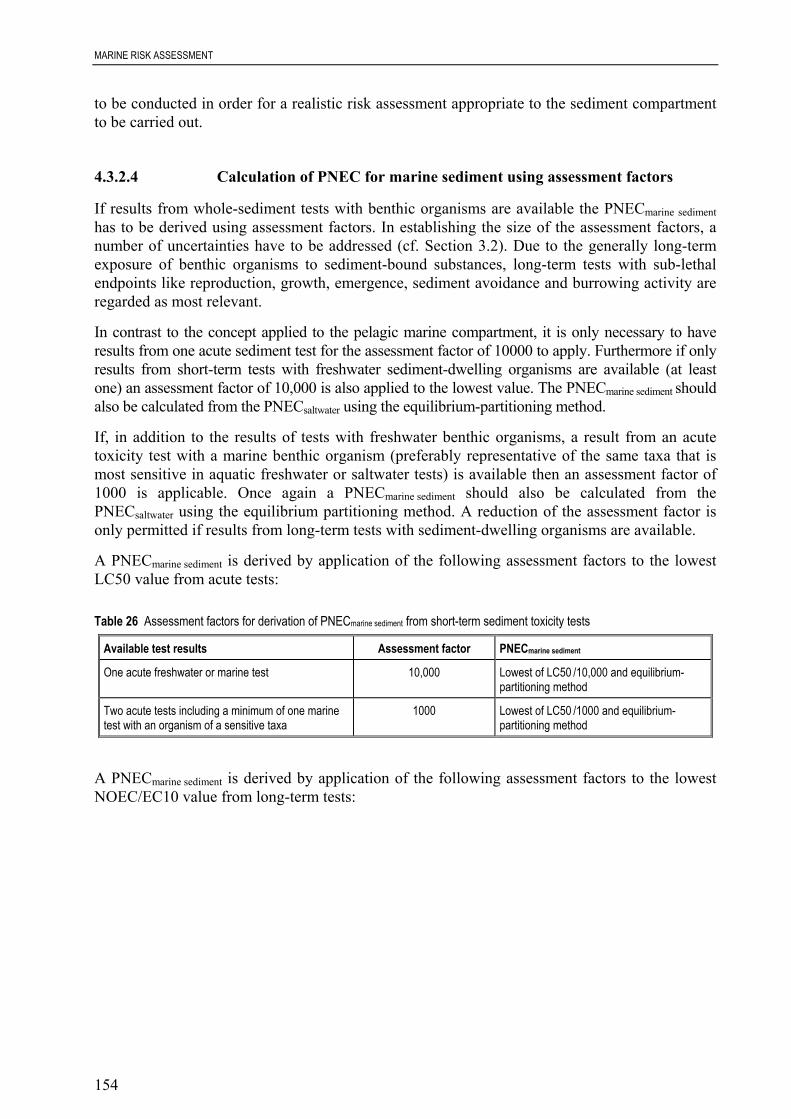
MARINE RISK ASSESSMENT
154
to be conducted in order for a realistic risk assessment appropriate to the sediment compartmentto be carried out.
4.3.2.4 Calculation of PNEC for marine sediment using assessment factors
If results from whole-sediment tests with benthic organisms are available the PNECmarine sedimenthas to be derived using assessment factors. In establishing the size of the assessment factors, anumber of uncertainties have to be addressed (cf. Section 3.2). Due to the generally long-termexposure of benthic organisms to sediment-bound substances, long-term tests with sub-lethalendpoints like reproduction, growth, emergence, sediment avoidance and burrowing activity areregarded as most relevant.
In contrast to the concept applied to the pelagic marine compartment, it is only necessary to haveresults from one acute sediment test for the assessment factor of 10000 to apply. Furthermore if onlyresults from short-term tests with freshwater sediment-dwelling organisms are available (at leastone) an assessment factor of 10,000 is also applied to the lowest value. The PNECmarine sediment shouldalso be calculated from the PNECsaltwater using the equilibrium-partitioning method.
If, in addition to the results of tests with freshwater benthic organisms, a result from an acutetoxicity test with a marine benthic organism (preferably representative of the same taxa that ismost sensitive in aquatic freshwater or saltwater tests) is available then an assessment factor of1000 is applicable. Once again a PNECmarine sediment should also be calculated from thePNECsaltwater using the equilibrium partitioning method. A reduction of the assessment factor isonly permitted if results from long-term tests with sediment-dwelling organisms are available.
A PNECmarine sediment is derived by application of the following assessment factors to the lowestLC50 value from acute tests:
Table 26 Assessment factors for derivation of PNECmarine sediment from short-term sediment toxicity tests
Available test results Assessment factor PNECmarine sediment
One acute freshwater or marine test 10,000 Lowest of LC50 /10,000 and equilibrium-partitioning method
Two acute tests including a minimum of one marinetest with an organism of a sensitive taxa
1000 Lowest of LC50 /1000 and equilibrium-partitioning method
A PNECmarine sediment is derived by application of the following assessment factors to the lowestNOEC/EC10 value from long-term tests:

MARINE RISK ASSESSMENT
155
Table 27 Assessment factors for derivation of PNECmarine sediment from long-term sediment toxicity tests
Available test results Assessment factor a)
One long-term freshwater sediment test 1000
Two long-term freshwater sediment tests with species representing different living and feeding conditions 500
One long-term freshwater and one saltwater sediment test representing different living and feedingconditions
100
Three long-term sediment tests with species representing different living and feeding conditions 50
Three long-term tests with species representing different living and feeding conditions including a minimumof two tests with marine species
10
a) The general principles of notes (c) and (d) as applied to data on aquatic organisms (Section 4.3.1.3) shall also apply to sediment data.Additionally, where there is convincing evidence that the sensitivity of marine organisms is adequately covered by that available fromfreshwater species, the assessment factors used for freshwater sediment data may be applied. Such evidence may include data from long-term testing of freshwater and marine aquatic organisms, and must include data on specific marine taxa.
If no results from long-term tests with sediment organisms are available and the PEC/PNEC ratioderived from the results of short-term sediment tests or via the equilibrium partitioning methodis a cause for concern then the need for long-term testing with sediment organisms should beconsidered.
Since there are no chronic marine sediment test methods that are internationally accepted theresults from any tests should always be carefully evaluated. Several factors can contribute tovariability in test results. Of major importance to sediment tests are the effects of grain size andorganic carbon content of the sediment on the bioavailability of a substance. Sediment grain sizecan also be an important factor in tests for other reasons. For example, the extent to whichbacteria can be adsorbed onto the sediment varies with particle size. Likewise, different speciesof amphipods prefer sediments with different particle size distributions. No satisfactory solutionto the question which reference sediment should be considered appropriate is therefore currentlyavailable. One should thus consider the tolerance of a given species with regard to the grain sizedistribution of the sediments in question. Also spiking techniques have to be optimised becauseoften water is spiked after spiking the sediment. In addition, more insight is needed in the uptakeroute of sediment bound contaminants in the organisms (exposure assessment).
Next to standardisation and test guidelines, it is necessary to further investigate the sensitivity,reproducibility and inter-laboratory variability of the tests. It must be mentioned that mostavailable data on these facts concern the tests applied on field sediments, and not on spikedsediments.
Examples of sub-chronic and chronic toxicity tests with whole sediment are given in Table 28.Most of the tests have been developed for amphipods and polychaetes and some of them arerecommended by the OECD (1998a). There is a need for chronic tests to be developed forMollusca. Early life-stage tests with mussels and oysters are available for testing aqueous phasesbut no standardised test is available for testing whole marine sediment samples. Chronic teststhat measure effects on community structure are also available but these tests seem to be veryinsensitive. Functional endpoints tests, e.g. nutrient release rates, have been used to assess theeffects of contaminated sediments (Dahllöff et al., 1999).
A final point that should be borne in mind is that single-species toxicity tests do not take accountof the interactions between the sediment inhabiting fauna and the fate or behaviour of chemicalsubstances, caused by e.g. bioturbation (Ciarelli et al., 1999; 2000). No procedures are currently

MARINE RISK ASSESSMENT
156
available for assessing the significance of such interactions but it is clear that they could be ofpotential significance, particularly in respect of the bioavailability of a sediment contaminant.
Table 28 Acute and chronic whole sediment toxicity tests
Test organism Acute orchronic test
Duration Endpoints Reference
AMPHIPODS
Corophium sp. (C.volutator or C.arenarium)
Chronic 28d survival,growth andreproduction
ASTM (1993),Environment Canada(Burton, 1992),
(OECD, 1998arecommended)
Degrader. Organisms can be fieldcollected. Cultivation causesintermediate to high expenses
Organism does not like coarsesediment.
Low concern with regard to animalwelfare
Ecologically important organismsrelevance for exposed ecosystemshigh.
SOP 1) available with field-collectedorganisms.
Ringtested
Leptocheirusplumulosus
chronic 28 d survival,
growth andreproduction
ASTM (1993),Environment Canada(Burton, 1992),US EPA (1996)
Degrader
grain size has a significant effect onsurvival, growth and reproduction.Survival is highest between 25%clay and 75% sand.
Low concern with regard to animalwelfare Ecologically importantorganisms relevance for exposedecosystems very high
SOP 1) available with field-collectedorganisms.
Ringtested
POLYCHAETES
Nereis/Neanthes spNeanthesarenaceodentatakancultivated
subacute/chronic
12 d - 28 d survival -survival/growth
ASTM (1994) Distributed widely throughout theworld.
Can be cultivated on the laboratorydegrader Low concern with regardto animal welfare relevance forexposed ecosystems very high.
SOP 1) available, equipment and testspecies commercially available.
Ringtested.
Table 28 continued overleaf

MARINE RISK ASSESSMENT
157
Table 28 continued Acute and chronic whole sediment toxicity tests
Test organism Acute orchronic test
Duration Endpoints Reference
POLYCHAETES (continued)
Arenicola marina chronic 28 d Survival ASTM (1994)
(OECD, 1998arecommended)
Degrader, wide tolerance ofsediment grain size. Organism isfound extensively over the OSPARand Helsinki conventions area;cultivation is difficult Low concernwith regard to animal welfarerelevance for exposed ecosystemsvery high.
SOP 1) available, equipment and testspecies commercially available.
Ringtested.
Arenicola marina subacute 10 Casting rate Thain and Bifield (2001) see above row .
Changes in feeding rate haveconsequences for sedimentcommunities.
SOP 1) available, equipment and testspecies commercially available.
OSPAR ringtested
ECHINODERMES
Echinocardiumcordatum
acute/subchronic
14 d Survival Stronkhorst, in press
(OECD, 1998arecommended)
Degrader, SOP 1) available withfield-collected organisms
Ringtested
MICROCOSM
Nematodes chronic 60 d communitystructure
(Austen andSomerfield, 1997)
1) Standard operating procedure
4.3.3 Assessment of secondary poisoning
4.3.3.1 Introduction
The assessment of the potential impact of substances on top predators in the marine environmentcan be based, in principle, on the same methodology as that used for a freshwater scenario. Aswith freshwater ecosystems the accumulation of hydrophobic chemicals through the marine foodchains may follow many different pathways along different trophic levels. This accumulationmay result in toxic concentrations in predatory birds or mammals ingesting aquatic biotacontaining the chemical. This effect is called secondary poisoning and should in principle beassessed by comparing the measured or estimated concentrations in the tissues and organs of thetop predators with the no-effect concentrations for these predators expressed as the internal dose.In practice, however, data on internal concentrations in wildlife animals are hardly ever available

MARINE RISK ASSESSMENT
158
and most no-effect levels are expressed in term of concentrations of the food that the organismsconsume (i.e. in mg.kg-1 food). Therefore, the actual assessment is normally based on acomparison of the (predicted) concentration in the food of the top predator and the (predicted)no-effect concentration which is based on studies with laboratory animals. A distinction is madebetween the methodology used to assess the effects of substances whose effects can be relateddirectly to bioconcentration (direct uptake via water) and those where also indirect uptake via thefood may contribute significantly to the bioaccumulation.
Highly bioaccumulative substances have both a very high bioconcentration potential (log Kowtypically >4.5 or BCF > 500) and are also resistant to biotransformation in animals.Biomagnification of such chemicals (increased food chain accumulation) is a major risk to thetop predators of food webs, as the consumption of contaminated food is a major source ofcontaminants in predatory marine birds and mammals. In contrast the direct uptake of substancesfrom the environment (that is from water and sediment) is only of minor relevance (Biddingerand Gloss, 1984; Opperhuizen, 1991). Factors that make these very hydrophobic substances ofparticular concern to the marine environment include longer food chains, migratory andreproductive aspects that may cause especially high exposure of progeny of marine specieslikely, long-life of many marine predators, and a higher fat content. However, whilst steady statelevels in birds may be reached within weeks depending on the biological half-life of thechemical (Pearce et al., 1989), contamination levels in mammals may continually increase withage, with a plateau only being evident after several years (Thompson, 1990; Teigen et al., 1993).
No distinction can effectively be made between the spatial scales in the approach to theassessment since the predators will take food from sources spread across local and regionalmarine scenarios, as well as from the open sea. In the assessment it is therefore proposed to use aPECsaltwater based on the mean of the local and regional concentrations for the assessment of thelocal situation, and for the regional situation to apply a spatially broader scale. Given that marinepredators may have a wider range of foraging and that the regional sea concentrations willnormally be lower, this is considered as a reasonable worst-case assumption.
Bioaccumulation of metallic species is not considered explicitly in this section.
4.3.3.2 Assessment of bioaccumulation and secondary poisoning
The assessment scheme
The principal endpoints for the secondary poisoning assessment are the predators and toppredators that prey on organisms that are in direct contact with the marine aqueous phase andreceive the substances from this source. A relatively simple food chain is modelled whichconsists of the marine water phase, marine food, marine fish and two separate levels ofpredators. This food chain is visualised in Figure 16. As can be seen from this scheme risks forthree different trophic levels need to be assessed:
1. risks to marine fish: No specific calculation needs to be performed for estimating the risk tomarine fish as this is covered by the risk assessment for aquatic organisms.
2. risks to marine predators: The risk to marine predators is calculated as the ratio between theconcentration in their food (marine fish) and the no-effect concentration for oral intake(PNECoralpredator). The concentration in the marine fish (Cfish) is obtained frombioconcentration of the substance from the aqueous phase and (for very hydrophobicsubstances) as a result of bioaccumulation from the food the fish consumes (which consists
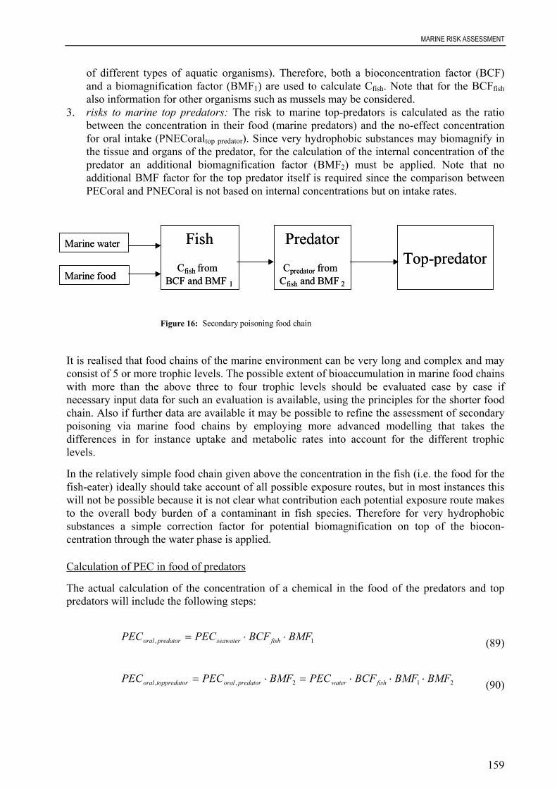
MARINE RISK ASSESSMENT
159
of different types of aquatic organisms). Therefore, both a bioconcentration factor (BCF)and a biomagnification factor (BMF1) are used to calculate Cfish. Note that for the BCFfishalso information for other organisms such as mussels may be considered.
3. risks to marine top predators: The risk to marine top-predators is calculated as the ratiobetween the concentration in their food (marine predators) and the no-effect concentrationfor oral intake (PNECoraltop predator). Since very hydrophobic substances may biomagnify inthe tissue and organs of the predator, for the calculation of the internal concentration of thepredator an additional biomagnification factor (BMF2) must be applied. Note that noadditional BMF factor for the top predator itself is required since the comparison betweenPECoral and PNECoral is not based on internal concentrations but on intake rates.
It is realised that food chains of the marine environment can be very long and complex and mayconsist of 5 or more trophic levels. The possible extent of bioaccumulation in marine food chainswith more than the above three to four trophic levels should be evaluated case by case ifnecessary input data for such an evaluation is available, using the principles for the shorter foodchain. Also if further data are available it may be possible to refine the assessment of secondarypoisoning via marine food chains by employing more advanced modelling that takes thedifferences in for instance uptake and metabolic rates into account for the different trophiclevels.
In the relatively simple food chain given above the concentration in the fish (i.e. the food for thefish-eater) ideally should take account of all possible exposure routes, but in most instances thiswill not be possible because it is not clear what contribution each potential exposure route makesto the overall body burden of a contaminant in fish species. Therefore for very hydrophobicsubstances a simple correction factor for potential biomagnification on top of the biocon-centration through the water phase is applied.
Calculation of PEC in food of predators
The actual calculation of the concentration of a chemical in the food of the predators and toppredators will include the following steps:
1, BMFBCFPECPEC fishseawaterpredatororal ⋅⋅= (89)
212,, BMFBMFBCFPECBMFPECPEC fishwaterpredatororalrtoppredatooral ⋅⋅⋅=⋅= (90)
Fish
C fish from BCF and BMF 1
Predator
Cpredator from Cfish and BMF 2
Top - predator Marine water
Marine food
Figure 16: Secondary poisoning food chain
Fish
C fish from BCF and BMF 1
Predator
Cpredator from Cfish and BMF 2
Top - predator Marine water
Marine food
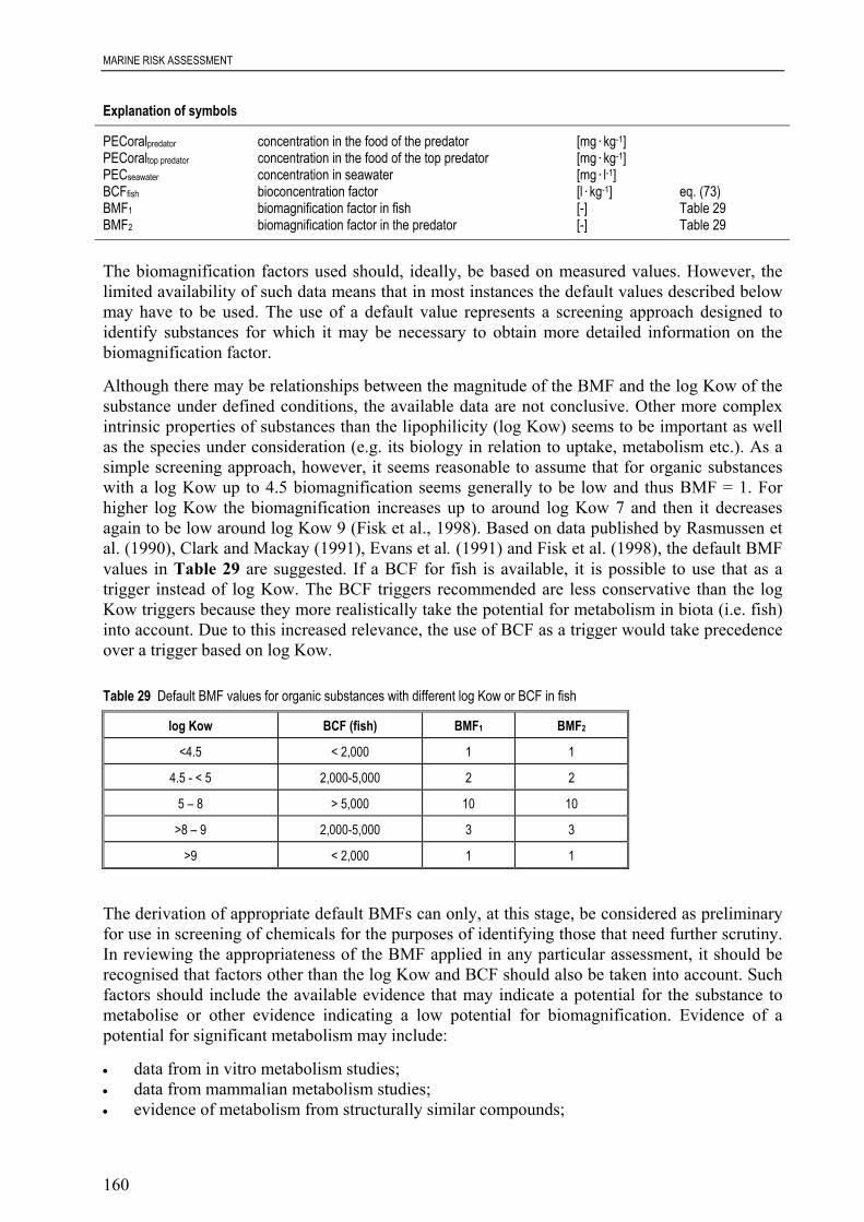
MARINE RISK ASSESSMENT
160
Explanation of symbols
PECoralpredator concentration in the food of the predator [mg.kg-1]PECoraltop predator concentration in the food of the top predator [mg.kg-1]PECseawater concentration in seawater [mg.l-1]BCFfish bioconcentration factor [l.kg-1] eq. (73)BMF1 biomagnification factor in fish [-] Table 29BMF2 biomagnification factor in the predator [-] Table 29
The biomagnification factors used should, ideally, be based on measured values. However, thelimited availability of such data means that in most instances the default values described belowmay have to be used. The use of a default value represents a screening approach designed toidentify substances for which it may be necessary to obtain more detailed information on thebiomagnification factor.
Although there may be relationships between the magnitude of the BMF and the log Kow of thesubstance under defined conditions, the available data are not conclusive. Other more complexintrinsic properties of substances than the lipophilicity (log Kow) seems to be important as wellas the species under consideration (e.g. its biology in relation to uptake, metabolism etc.). As asimple screening approach, however, it seems reasonable to assume that for organic substanceswith a log Kow up to 4.5 biomagnification seems generally to be low and thus BMF = 1. Forhigher log Kow the biomagnification increases up to around log Kow 7 and then it decreasesagain to be low around log Kow 9 (Fisk et al., 1998). Based on data published by Rasmussen etal. (1990), Clark and Mackay (1991), Evans et al. (1991) and Fisk et al. (1998), the default BMFvalues in Table 29 are suggested. If a BCF for fish is available, it is possible to use that as atrigger instead of log Kow. The BCF triggers recommended are less conservative than the logKow triggers because they more realistically take the potential for metabolism in biota (i.e. fish)into account. Due to this increased relevance, the use of BCF as a trigger would take precedenceover a trigger based on log Kow.
Table 29 Default BMF values for organic substances with different log Kow or BCF in fish
log Kow BCF (fish) BMF1 BMF2
<4.5 < 2,000 1 1
4.5 - < 5 2,000-5,000 2 2
5 – 8 > 5,000 10 10
>8 – 9 2,000-5,000 3 3
>9 < 2,000 1 1
The derivation of appropriate default BMFs can only, at this stage, be considered as preliminaryfor use in screening of chemicals for the purposes of identifying those that need further scrutiny.In reviewing the appropriateness of the BMF applied in any particular assessment, it should berecognised that factors other than the log Kow and BCF should also be taken into account. Suchfactors should include the available evidence that may indicate a potential for the substance tometabolise or other evidence indicating a low potential for biomagnification. Evidence of apotential for significant metabolism may include:
• data from in vitro metabolism studies;• data from mammalian metabolism studies;• evidence of metabolism from structurally similar compounds;

MARINE RISK ASSESSMENT
161
• a measured BCF significantly lower than predicted from the log Kow, indicating possiblemetabolism.
Where evidence exists suggesting that such metabolism may occur, the BMF detailed above maybe reduced. Where such reductions are proposed, a detailed justification must be provided.
Application of different spatial scales
Apart from the fact that for the assessment of the risks to the top predator an additionalbiomagnification factor is used the assessment also differs in terms of the input values that areused for the seawater concentrations that lead to the concentrations in the food of the differentpredators. For the first tier (or trophic level) of predators a worst-case assumption is that theyobtain their prey equally from the local and regional area, respectively. This is in line with theassessment for freshwater and terrestrial organisms where a similar choice is made. For thecalculation of the PECoral for the predators this implies the following:
( )seawaterannseawaterseawater lPECregionaPEClocalPEC +⋅= ,5.0 (91)
When PECseawater is substituted in equation 89 this results in the following equation:
( ) 1,, 5.0 BMFBCFlPECregionaPEClocalPEC fishseawaterannseawaterpredatororal ⋅⋅⋅+= (92)
Explanation of symbols
PECoralpredator concentration in the food of the predator [mg.kg-1]PECseawater concentration in seawater [mg.l-1]BCFfish bioconcentration factor [l.kg-1] eq. (73)BMF1 biomagnification factor in fish [-] Table 29PECregionalseawater predicted environmental concentration in the region [mg.l-1]PEClocalseawater,ann annual average predicted environmental concentration [mg.l-1]
For the second tier of organisms, the top predators, it can be assumed that they obtain their preymainly from the larger-scale regional marine environment which is to a lesser extent influencedby point source discharges. However, since it cannot be ruled out that certain top predators preyon organisms that receive their food from relatively small areas it is proposed to assume, as arealistic worst case, a 90/10 ratio between regional and local food intake. For the calculation ofthe oral intake rate for the top predator (PECoraltop predator) this implies:
seawaterannseawaterwater lPECregionaPEClocalPEC ⋅+⋅= 9.01.0 , (93)
When PECwater is substituted in equation 90 this results in the following equation:
( ) 21,, 9.01.0 BMFBMFBCFlPECregionaPEClocalPEC fishseawaterannseawaterpredatortoporal ⋅⋅⋅⋅+⋅=− (94)
MARINE RISK ASSESSMENT
162
Derivation of the PNECoral values
In the derivation of the PNECoral values only toxicity studies reporting on dietary and oralexposure are relevant as the pathway for secondary poisoning refers exclusively to the uptake ofchemicals through the food chain. However, reliable toxicity data for predatory marine birds(such as gulls and penguins) and mammals (such as seals, dolphins, whales and polar bears) areextremely limited (Nendza et al., 1997). Furthermore, testing of such species would be ethicallyunsound and contrary to animal welfare concerns. Therefore, it is necessary to extrapolatethreshold levels for marine species from terrestrial species assuming there are interspeciescorrelations between laboratory bird species and marine predatory bird species, and betweenlaboratory mammals (e.g. rats) and the considerably larger marine predatory mammals. Thisprocedure is identical to that applicable for other media (see Section 3.8.3.5).
4.3.3.3 Testing strategy
If the PEC/PNEC ratio based on use of default BMF values indicates potential problems at anytrophic level it should first be considered whether a refinement of the PEC-assessment ispossible, i.e. the release and exposure assessment, including the fate related parameters such asdetermination of log Kow or BCF. In special cases it may even be considered to start withbioaccumulation studies in fish to determine the assimilation coefficient and the biological half-life of the substance (i.e. to determine BMF1) prior to estimating or determining thebioconcentration factor (BCF). Also a refinement of the PNECoral could be considered, i.e. torequire a long-term feeding study with laboratory mammals or birds to derive a more realisticNOECoral value. In conducting such a study according to current test methods, it may in specialcases be considered whether to extend such studies to include satellite groups for determinationof the concentration of the substance in the animals during exposure (i.e. to measureBMF2 values). Alternatively or supplementary to actual testing can be monitoring of biota forwhich it is clear that they have lived in the environment that is covered in the assessment. Ofcourse no active sampling of (top)predators should be performed, but for instance animals thatare found dead can be used to get an indication about possible biomagnification factors inwildlife. Useful information might also be obtained from eggs or from biopsies of skin orblubber of marine birds or mammals.
4.4 PBT ASSESSMENT
4.4.1 Introduction
The PBT assessment is considered to be different from the local and regional assessmentapproaches, as it seeks to protect ecosystems where the risks are more difficult to estimate.These additional concerns for the marine environment, which may not be adequately addressedby the traditional risk assessment methodologies, can be summarised as:
a. the concern that hazardous substances may accumulate in parts of the marine environmentand that:
(i) the effects of such accumulation are unpredictable in the long-term;(ii) that such accumulation would be practically difficult to reverse;

MARINE RISK ASSESSMENT
163
b. the concern that remote areas of the oceans should remain untouched by hazardoussubstances resulting from human activity, and that the intrinsic value of pristineenvironments should be protected.
These concerns particularly occur with substances that can be shown both to persist for longperiods and bioaccumulate in biota, and can give rise to toxic effects after a greater time and at agreater distance than chemicals without these properties. While this is also true for thefreshwater environment, the additional concern in the marine environment is that once thechemical has entered the open seas, any cessation of emission will not necessarily result in areduction in chemical concentration and hence any effects become difficult to reverse. Equally,because of the long-term exposures and long-life-cycle of many important marine species,effects may be difficult to detect at an early stage.
For PBT substances a “safe” concentration in the environment cannot be established with sufficientreliability. The PBT assessment is particularly developed to take into account the unacceptable highuncertainty in predicting reliable exposure and/or effect concentrations hampering quantitative riskassessment. The PBT assessment basically consists of two different steps:
• identification of PBT substances using specific criteria for the inherent properties; and • an evaluation of the sources, major emissions and pathways to the marine environment to
sufficiently establish the most appropriate and effective measures to reduce the releases tothe marine environment.
The urgency and stringency of possible measures may, however, be dependent on the potentialof the substance to be transported to the open sea. This can be assessed qualitatively byconsidering the use pattern, volumes and emissions or by using measured data. Openapplications and wide dispersive uses of the substance are regarded particularly relevant as wellas non-minimised direct discharges from production, formulation and industrial use.
4.4.2 PBT criteria
The criteria to be used to decide if a substance must be regarded as a PBT substance aresummarised in Table 30 below. The testing strategies to obtain the data that are necessary todecide whether a substance fulfils these criteria are given in separate sections on persistence,bioaccumulation and toxicity. The table contains two sets of criteria, one for PBT substances anda second category for so-called very persistent and very bioaccumulating substances (vPvB).This second category is developed under the recognition that for substances that are verypersistent and bioaccumulate significantly in the food chain, high but unpredictable levels maybe reached in wildlife or man over extended time periods. For such substances it is not necessaryto demonstrate toxicity in laboratory testing as long-term effects can be anticipated anyway.
For most substances the available data will not allow to come to a definitive answer to thequestion if the substance must be considered under the PBT assessment. Hence screening datathat identify whether the substance has a potential to be a PBT have to be made use of. Thetesting strategies in the following paragraphs should be followed and further information shouldbe asked for accordingly. In deciding which information is requested (on P, B or T) care must betaken to avoid animal testing where possible. This implies that when for several propertiesfurther information is needed the assessment should be focussed on clarifying the potential forpersistence first. When it is clear that the P criterion is fulfilled a stepwise approach should befollowed to elucidate the B criterion, eventually followed by toxicity testing to clarify the Tcriterion.

MARINE RISK ASSESSMENT
164
Table 30 Criteria for identification of PBT and vPvB substances
Criterion PBT criteria vPvB-criteria
P Half-life > 60 d in marine water or > 40 d in freshwater*or half-life > 180 d in marine sediment or > 120 d infreshwater sediment*
Half-life > 60 d in marine- or freshwater or >180 d inmarine or freshwater sediment
B BCF > 2,000 BCF > 5,000
T Chronic NOEC < 0.01 mg/l or CMR or endocrinedisrupting effects
Not applicable
* For the purpose of marine environmental risk assessment half-life data in freshwater and freshwater sediment can be overruled by dataobtained under marine conditions.
In principle, substances are selected when they fulfil the criteria for all three inherent propertiesP, B and T. However, certain flexibility is required in their application for instance in caseswhere one criterion is marginally not fulfilled but the others are exceeded considerably. Thismay include for example substances that do not fulfil the persistence criteria but bioaccumulatesignificantly and are measured in marine biota distant from anthropogenic sources.
It is realized that the individual trigger values may be scientifically disputable when consideredin isolation. However, by applying the combined set of criteria it is expected that substances willbe selected for which quantification of the risk by using the PEC/PNEC approach is consideredtoo uncertain.
The PBT assessment has links to similar concepts discussed in other fora (e.g. the UNEPStockholm Convention on Persistent Organic Pollutants, the OSPAR Hazardous SubstancesStrategy (OSPAR, 1998)). The discussions from the other fora have been carefully considered.
4.4.3 Testing strategy for the P criterion
4.4.3.1 Introduction
The persistence of a substance reflects the potential for long-term exposure of organisms but alsothe potential for the substance to reach the marine environment and to be transported to remoteareas. The assessment of the (potential for) persistency in the marine environment should inprinciple be based on actual half-life data determined under marine environmental conditions.Depending on whether a substance has a half-life smaller or greater than the cut-off criterion it isdecided if a substance fulfils the P criterion. When these key data are not available other types ofavailable information on the degradability of a substance can be used to decide if further testingis needed to assess the potential persistence. In this approach three different levels of informationare defined according to their perceived relevance to the criteria:
• experimental data on persistence in the marine environment;• other experimental data;• data from biodegradation estimation models.
An explanation on what type of information is relevant within these levels and the relevant cut-off values is given below. It must be noted that this approach reflects existing knowledge onbiodegradation and should be considered as a pragmatic approach to make optimal use of theavailable data and methods. Clearly, more research is needed to better estimate the persistence inthe marine environment from existing biodegradation tests. Moreover, other degradation
MARINE RISK ASSESSMENT
165
mechanisms such as hydrolysis and photolysis should be taken into account where they can beshown to be relevant.
4.4.3.2 Experimental data on persistence in the marine environment
In principle the persistence in the marine environment should be assessed in simulation testsystems that determine the half-life under relevant environmental conditions. The determinationof the half-life should include assessment of metabolites with PBT-characteristics. The half-lifeshould be used as the first and main criterion in order to determine whether substances should beregarded as persistent. Hence appropriate half-life data from valid simulation tests override datafrom the other levels of information. Substances with a half-life in marine water of > 60 days ora half-life of >180 days in marine sediment are considered as being persistent. Substances areconsidered very persistent (vP) when the half-life in marine or freshwater is > 60 days or thehalf-life in marine or freshwater sediments is > 180 days.
Recommended simulation test methods for water and sediment are described in Section 4.2.3.3.
Tests performed under marine conditions should use media from marine areas not directlyinfluenced by freshwater outlets or runoffs. This means that samples taken for inoculation andconduction of marine biodegradation simulation tests must not contain significant amounts offreshwater microorganisms as these to a larger extent could already have been pre-exposed oradapted to the substance. It is not possible to establish specific criteria and each test must beevaluated case-by-case. However, the content of freshwater in the sample should be low (i.e. alarge dilution as e.g. determined by salinity), the sample should be taken from the water column(and not the surface), the content of microorganisms should be low (compared to freshwater) andcross-contamination during handling, transport and testing should be avoided.
4.4.3.3 Other experimental data
In case no half-life data are available for marine water or sediment the decision whether asubstance is potentially persistent needs to be based on other experimental data. If available, usecan be made of the half-life values from simulation tests of degradation in freshwater. Since thedegradation in marine waters other than estuaries is expected to be slower than in freshwater acriterion of >40 days for freshwater and >120 days for freshwater sediments has to be used.
Where no data are available which allow the assignment of a degradation half-life in theenvironment based on simulation test data, other experimental data may be considered. Theavailable information relating to biodegradability is dominated by test results on ReadyBiodegradability (EU Annex V C.4 A, C, E and F; OECD guidelines 301A-D, 1992f, 306, 1992eor equivalent) and to a lesser extent by data on the Inherent Biodegradability (EU Annex V C.12and C.9; OECD TG A-C, 1981d or equivalent). The conditions for degradation in the marineenvironment are far from the conditions applied in these standard tests (cf. Section 4.2.3). Hence,extrapolation of the existing biodegradation information (either measured data from ready andinherent tests or results from QSAR modelling) to degradation rates in the marine environment isvery difficult and care should be taken not to over-interpret the outcome of such tests. However,in order to use the available information to select potentially persistent substances, thisinformation should be used in the following way:
• readily biodegradable substances (fulfilling or not fulfilling the 10-day window criterion)are considered as not persistent in the PBT assessment;
MARINE RISK ASSESSMENT
166
• when a substance does not fulfil the criteria for ready biodegradability as defined in sectionson biodegradation and for the marine ready test (see Sections 2.3.6 and 4.2.3.4), it isconsidered as being potentially persistent. The 10-day window criterion should not be usedhere as an additional criterion. If the substance fulfils the criteria for B and T, further testingis needed. It must be noted that in this case it is not considered appropriate to performinherent biodegradability tests but rather to go directly to simulation testing;
• when results are available showing that a substance does not fulfil the criteria for inherentbiodegradability as defined within the Annex V method or the OECD guideline this is aclear indication that the substance will not biodegrade in the marine environment either. Thesubstance will be regarded as potentially persistent. When the (screening) criteria for B andT are also fulfilled, further testing is needed in order to determine the half-life in theenvironment.
• when a substance passes the criteria for inherent biodegradability tests this does notnecessarily indicate that it will not be persistent under environmental conditions. However,in order to make the best use of available information it is accepted to use the results of twospecific tests when they fulfil certain criteria as an indication that the substance is notpersistent. These test are:- Zahn-Wellens Test (EU Annex V C.9, OECD 302B, 1992g): Pass level (70%
mineralisation) must be reached within 7 days, log-phase should be no longer than 3days, percentage removal in the test before degradation occurs should be below 15%,not tested with pre-adapted microorganisms;
- MITI II -test (OECD 302C, 1981d): Pass level must be reached within 14 days; log-phase should be no longer than 3 days, not tested with pre-adapted microorganisms.
In case a range of biodegradation data, including conflicting data, is available, a case-by-caseassessment is needed, using a weight of evidence approach, in order to decide whether asubstance has the potential to be persistent (see also Section 2.3.6).
4.4.3.4 Data from biodegradation estimation models
For new substances, priority existing substances and biocides, information from a readybiodegradability test is normally available and therefore an initial decision whether the substanceis potentially persistent can be taken. However, for many other substances no data will beavailable or the available information is difficult to interpret. For these substances it can behelpful to apply models that estimate the potential for biodegradation in the environment.
In a preliminary assessment whether a substance has a potential for persistence in the marineenvironment and hence for asking for actual test data it is proposed to consider use of theBIOWIN program. This program estimates aerobic biodegradability of organic chemicals using6 different models:
1. linear model,2. non-linear model,3. ultimate biodegradability timeframe model,4. primary biodegradability timeframe model,5. MITI linear model,6. MITI non-linear model;

MARINE RISK ASSESSMENT
167
The use of the results of these programs in a conservative way may fulfil the needs forevaluating the potential for persistency. The use of three out of the six models is suggested asfollows:
• non-linear model prediction: does not biodegrade fast (<0.5) or• MITI non-linear model prediction: not readily degradable (<0.5) and• ultimate biodegradation timeframe prediction: > months (<2.2)
When predictions of these three models are combined relatively few not readily biodegradablesubstances will not be identified, without in the same time causing a significant increase in thenumber of falsely included readily biodegradable substances.
The preliminary character of this method to identify potentially persistent substances in themarine environment is emphasised, and further possible development of a suitable methodologyis recommended. The BIOWIN program is available from the US EPA's internet site(http://www.epa.gov/oppt/exposure/docs/episuitedl.htm).
4.4.3.5 Summary of the P assessment
A summary of the assessment of biodegradation data in the context of the P criterion is given inTable 31 below.
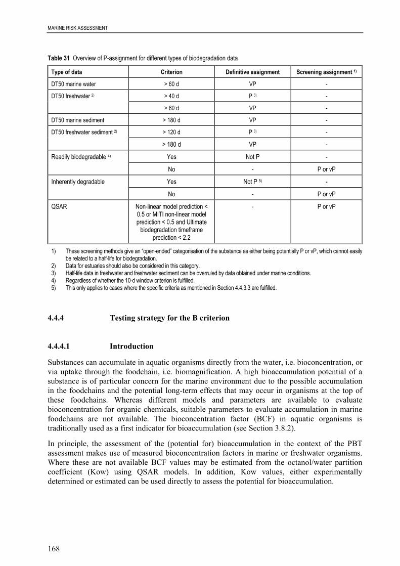
MARINE RISK ASSESSMENT
168
Table 31 Overview of P-assignment for different types of biodegradation data
Type of data Criterion Definitive assignment Screening assignment 1)
DT50 marine water > 60 d VP -
> 40 d P 3) -DT50 freshwater 2)
> 60 d VP -
DT50 marine sediment > 180 d VP -
> 120 d P 3) -DT50 freshwater sediment 2)
> 180 d VP -
Yes Not P -Readily biodegradable 4)
No - P or vP
Yes Not P 5) -Inherently degradable
No - P or vP
QSAR Non-linear model prediction <0.5 or MITI non-linear modelprediction < 0.5 and Ultimate
biodegradation timeframeprediction < 2.2
- P or vP
1) These screening methods give an “open-ended” categorisation of the substance as either being potentially P or vP, which cannot easilybe related to a half-life for biodegradation.
2) Data for estuaries should also be considered in this category.3) Half-life data in freshwater and freshwater sediment can be overruled by data obtained under marine conditions.4) Regardless of whether the 10-d window criterion is fulfilled.5) This only applies to cases where the specific criteria as mentioned in Section 4.4.3.3 are fulfilled.
4.4.4 Testing strategy for the B criterion
4.4.4.1 Introduction
Substances can accumulate in aquatic organisms directly from the water, i.e. bioconcentration, orvia uptake through the foodchain, i.e. biomagnification. A high bioaccumulation potential of asubstance is of particular concern for the marine environment due to the possible accumulationin the foodchains and the potential long-term effects that may occur in organisms at the top ofthese foodchains. Whereas different models and parameters are available to evaluatebioconcentration for organic chemicals, suitable parameters to evaluate accumulation in marinefoodchains are not available. The bioconcentration factor (BCF) in aquatic organisms istraditionally used as a first indicator for bioaccumulation (see Section 3.8.2).
In principle, the assessment of the (potential for) bioaccumulation in the context of the PBTassessment makes use of measured bioconcentration factors in marine or freshwater organisms.Where these are not available BCF values may be estimated from the octanol/water partitioncoefficient (Kow) using QSAR models. In addition, Kow values, either experimentallydetermined or estimated can be used directly to assess the potential for bioaccumulation.
MARINE RISK ASSESSMENT
169
4.4.4.2 Assessment of measured BCF data
The decision whether or not a substance fulfils the B criterion should in principle be based onmeasured data on bioconcentration in aquatic species. Data from freshwater as well as marinespecies can be used. Extensive guidance on the quality assessment of such data can be foundelsewhere (e.g. OECD, 2001c). A substance is considered to fulfil the B criterion when themeasured BCF on a wet weight basis exceeds a value of 2,000. A substance is considered verybioaccumulative (vB) when the BCF exceeds a value of 5,000.
4.4.4.3 Assessment of the potential for bioaccumulation
When measured BCF values are not available the Kow or the BCF based on modelling can beused to indicate the liability to bioaccumulate from water. For substances with log Kow < 6assessment on the basis of Kow or estimated BCF does not make a real difference since allavailable BCF models are linear (see Section 3.8.3.2). The B criterion for log Kow is thereforedirectly derived from this linear relationship. A substance is considered to potentially fulfil the Bcriterion when log Kow exceeds a value of 4.5.
For highly hydrophobic substances, e.g. with log Kow > 6, experimentally derived BCF valuestend to decrease with increasing log Kow. Several conceptual explanations as well asexplanations referring to experimental artefacts can be given for this decline. For thesesubstances the available BCF models can lead to very different results. As a consequence thepotential for bioaccumulation is assessed by expert judgement on the basis of the log Kow valueand the estimated BCF using the available BCF models. Such an assessment must be done on acase-by-case basis taking into account what is known about the BCF QSAR-models and thespecific properties of the substance, in particular what is known to affect uptake and the potentialfor metabolism in aquatic organisms. Care must be taken that substances with high log Kowvalues are not deleted from selection processes without applying expert judgement to them.
It must be noted that for priority existing substances, new substances and biocides a measuredoctanol/water partition coefficient is usually available. Additionally a range of QSAR modelscan be used to estimate this parameter (see e.g. Chapter 4, Meylan et al., 1999; OECD, 2001c).
4.4.4.4 Other information relevant for assessment of the B criterion
In addition to the above-mentioned data on bioconcentration or bioaccumulation in aquaticspecies evidence that a substance shows high bioaccumulation in other species may also be usedto decide whether the B criterion is fulfilled. Such evidence may be based on information fromspecific laboratory tests or from field studies. Specific attention needs to be paid to measureddata in biota. Measured data in biota are a clear indicator that a substance is taken up by anorganism. However, they are not an indicator that significant bioconcentration orbioaccumulation has occurred. The interpretation of such data in terms of actual bioaccumulationor biomagnification factors can especially be difficult when the sources and levels of theexposure (through water as well as through food) are not known or cannot be estimatedreasonably.

MARINE RISK ASSESSMENT
170
4.4.5 Testing strategy for the T criterion
4.4.5.1 Introduction
For persistent and bioaccumulative substances long-term exposure can be anticipated andexpected to cover the whole life-time of an organism and even multiple generations. Thereforechronic or long-term ecotoxicity data, ideally covering the reproductive stages should inprinciple be used for the assessment of the T criterion. In practice, however, the principal dataavailable for most chemicals will be for short-term effects, and this must, in the first instance, beused to drive initial selection. Mammalian toxicity data must also be considered in the selectiondue to the fact that toxic effects on top predators, including man may occur through long-termexposure via the food-chain. The selection criteria should therefore consider two types of effectdata, either of which will trigger selection.
4.4.5.2 Chronic effects data
A substance is considered to fulfil the toxicity criterion when:
• the long-term NOEC for marine or freshwater organisms is less than 0.01 mg/l. When otherinformation is available such as data on sediment toxicity or data from feeding studies thisneeds to be assessed on case-by-case basis. For biocides and pesticides results from sub-chronic, chronic or reproduction avian toxicity tests may be available. A chronic NOEC ofless than 30 mg/kg/food can be used as a criterion.
or• when the substance is classified as Carcinogenic, (category 1 & 2), Mutagenic (category 1 &
2) or Toxic for Reproduction (category 1, 2 & 3) or when there is evidence of chronictoxicity, as identified by the classifications T, R45, R46, R48, R60 and R61 or Xn, R48,R62, R63 and R64 8.
• when a substance is classified as Carcinogenic category 3 or Mutagenic category 3 a case-by-case assessment must be carried out to decide whether the evidence is sufficient for thesubstance to be considered as toxic, in the context of this PBT assessment, or whetherfurther information is needed to clarify this potential concern.
or • when there is substantiated evidence of long-term toxicity (e.g. endocrine disrupting
effects). Such evidence needs to be considered on a case-by-case basis.
4.4.5.3 Acute effects data (screening level)
Where data on chronic effects are not available short-term toxicity data for marine or freshwaterorganisms can be used to determine whether a substance is a potential PBT provided thescreening criteria for P and B are fulfilled. In the context of the PBT assessment a substance isconsidered to be potentially toxic when the L(E)C50 to aquatic organisms is less than 0.1 mg/l.If a substance is confirmed to fulfil the ultimate P and B criteria chronic toxicity data are
8 In relation to the use of R64 in the context of the PBT assessment care should be taken that the actual assignment
of the R-phrase is a result of results of one or two generation studies in animals which indicate the presence ofadverse effects on the offspring due to transfer in the milk (see Annex VI to Directive 67/548).
MARINE RISK ASSESSMENT
171
required to deselect this substance from being considered as a PBT. In principle chronic toxicitydata, when obtained for the same species, should override the results from the acute tests.
In the context of the PBT assessment acute mammalian toxicity tests are normally not considered toprovide an appropriate indication of chronic effects. However, it should be noted that when asubstance is classified as Very Toxic or Toxic after oral dosing (LD50 < 200 mg/kg bw/d) and thetoxicity is expected to be the result of systemic effects, the probability that the chronic NOAELafter repeated dosing (e.g. 28 d or 90 d) will be less than the trigger value for R48 (± 150 or50 mg/kg bw/d, respectively) will be high. The substance would therefore be classified andconsidered as fulfilling the T criterion. In that case verification of the actual chronic toxicity byperforming animal testing is not recommended. When the P and B screening criteria are alsofulfilled the substance can be considered as a PBT unless additional information indicatesotherwise.
4.4.5.4 Estimated effects data
In case where no acute or chronic toxicity data are available the assessment of the T criterion at ascreening level can be performed using data obtained from quantitative structure activityrelationships (QSARs). Guidance on the use of QSARs for specific groups of substances can befound in Chapter 4.
It must be noted that since long-term effects can be anticipated for very bioaccumulativesubstances (vPvB), further animal testing for such substances is deemed unnecessary.
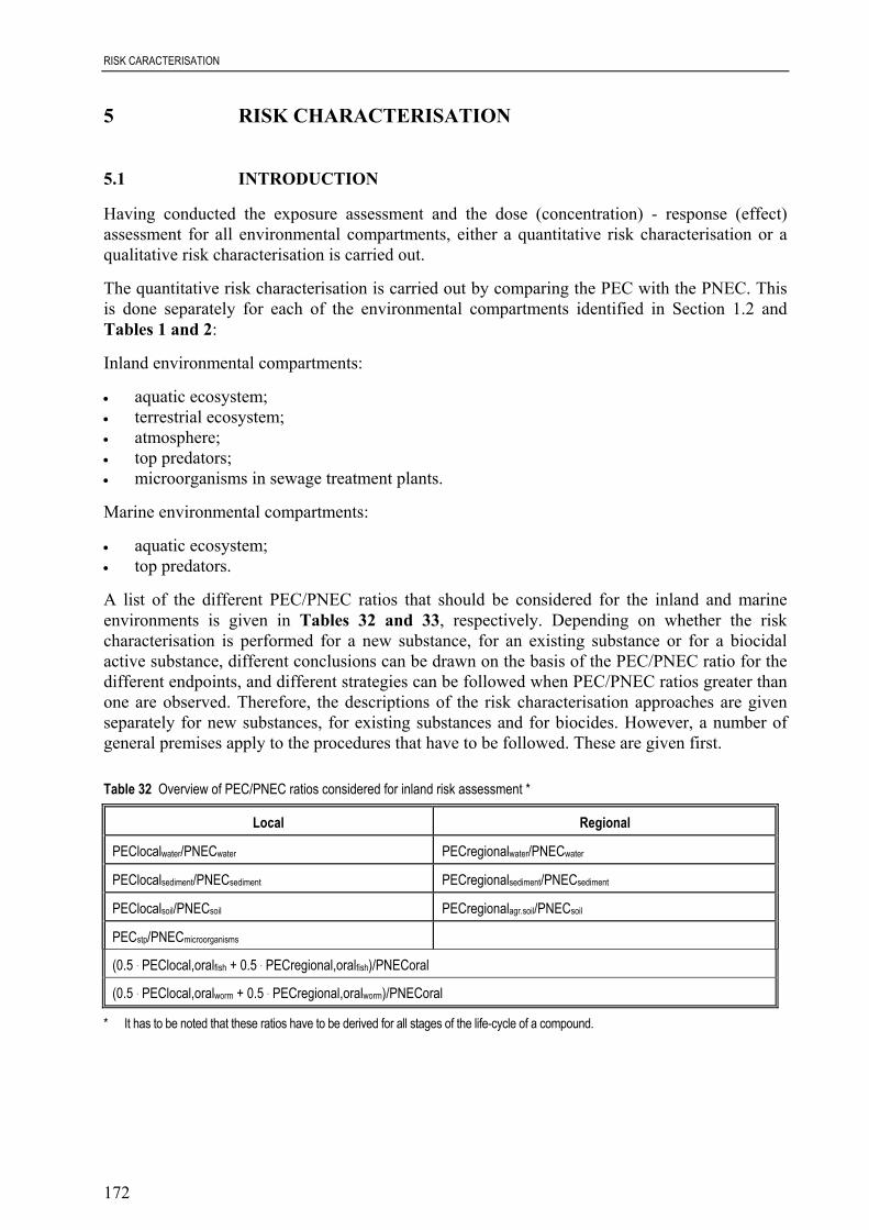
RISK CARACTERISATION
172
5 RISK CHARACTERISATION
5.1 INTRODUCTION
Having conducted the exposure assessment and the dose (concentration) - response (effect)assessment for all environmental compartments, either a quantitative risk characterisation or aqualitative risk characterisation is carried out.
The quantitative risk characterisation is carried out by comparing the PEC with the PNEC. Thisis done separately for each of the environmental compartments identified in Section 1.2 andTables 1 and 2:
Inland environmental compartments:
• aquatic ecosystem;• terrestrial ecosystem;• atmosphere;• top predators;• microorganisms in sewage treatment plants.
Marine environmental compartments:
• aquatic ecosystem;• top predators.
A list of the different PEC/PNEC ratios that should be considered for the inland and marineenvironments is given in Tables 32 and 33, respectively. Depending on whether the riskcharacterisation is performed for a new substance, for an existing substance or for a biocidalactive substance, different conclusions can be drawn on the basis of the PEC/PNEC ratio for thedifferent endpoints, and different strategies can be followed when PEC/PNEC ratios greater thanone are observed. Therefore, the descriptions of the risk characterisation approaches are givenseparately for new substances, for existing substances and for biocides. However, a number ofgeneral premises apply to the procedures that have to be followed. These are given first.
Table 32 Overview of PEC/PNEC ratios considered for inland risk assessment *
Local Regional
PEClocalwater/PNECwater PECregionalwater/PNECwater
PEClocalsediment/PNECsediment PECregionalsediment/PNECsediment
PEClocalsoil/PNECsoil PECregionalagr.soil/PNECsoil
PECstp/PNECmicroorganisms
(0.5 . PEClocal,oralfish + 0.5 . PECregional,oralfish)/PNECoral
(0.5 . PEClocal,oralworm + 0.5 . PECregional,oralworm)/PNECoral
* It has to be noted that these ratios have to be derived for all stages of the life-cycle of a compound.

RISK CHARACTERISATION
173
Table 33 Overview of PEC/PNEC ratios considered for marine risk assessment *
Local Regional
PEClocalseawater/PNECsaltwater PECregionalseawater/PNECsaltwater
PEClocalsediment/PNECmarine sediment PECregionalsediment/PNECmarine sediment
[(PEClocalseawater,ann + PECregionalseawater) · 0.5 · BCFfish · BMF1]/PNECoralpredator
[(0.1 · PEClocalseawater,ann + 0.9 · PECregionalseawater) · BCFfish · BMF1 · BMF2]/PNECoraltop predator
* It has to be noted that these ratios have to be derived for all stages of the life-cycle of a compound.
When no quantitative risk characterisation can be carried out, for example for remote marineareas or when either PEC or PNEC cannot be properly derived, a qualitative risk characterisationshould be conducted. This is described in Section 5.6.
5.2 GENERAL PREMISES FOR RISK CHARACTERISATION
In general, the risk characterisation phase is carried out along the following steps (seeFigure 17):
• determine the PEC/PNEC ratios for the different environmental compartments considered.
Dependent on these PEC/PNEC ratios:
• determine whether further information/testing may lead to a revision of these ratios;• ask for further information/testing when appropriate;• refine the PEC/PNEC ratio.
This iterative process should be continued until a final conclusion regarding the environmentalrisks can be reached.
For the risk characterisation for the aquatic and terrestrial ecosystems, including secondarypoisoning, a direct comparison of the PEC and PNEC values is carried out, presuming that therelevant data are available. If the PEC/PNEC ratio is greater than one the substance is “ofconcern” and further action has to be taken.
For the air compartment usually only a qualitative assessment of abiotic effects is carried out. Ifthere are indications that one or more of these effects occur for a given substance, expertknowledge should be consulted or the substance be handed over to the relevant internationalgroup, e.g. to the responsible body in the United Nations Environment Programme (UNEP) forozone depleting substances. In some cases also an assessment of the biotic effects to plants canbe carried out.
The risk characterisation for top predators is made by comparing the PECoral with the PNECoralin accordance with the procedure described in Sections 3.8 and 4.3.3. If the ratioPECoral / PNECoral is greater than one and a refinement of the PECoral or the PNECoral is notpossible or reasonable, risk reduction measures should be considered.
The risk characterisation for microorganisms in sewage treatment systems is done by comparingthe PECstp with the PNECmicroorganisms. If the ratio of these two values is greater than one, thisindicates that the substance may have a detrimental effect on the function of the STP andtherefore is “of concern”.
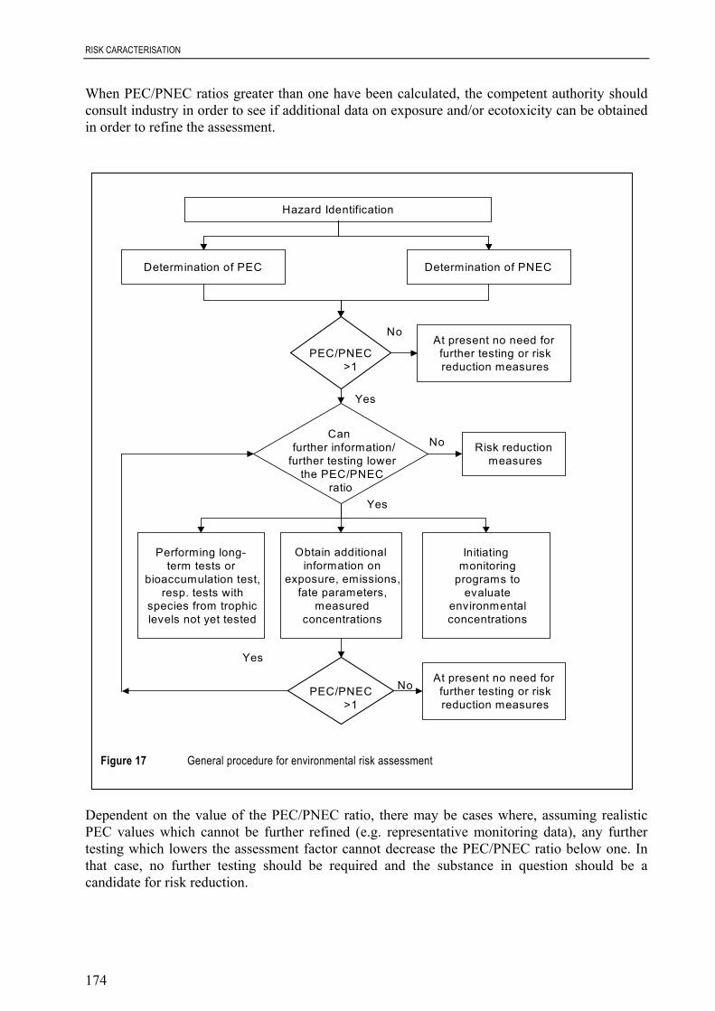
RISK CARACTERISATION
174
When PEC/PNEC ratios greater than one have been calculated, the competent authority shouldconsult industry in order to see if additional data on exposure and/or ecotoxicity can be obtainedin order to refine the assessment.
Dependent on the value of the PEC/PNEC ratio, there may be cases where, assuming realisticPEC values which cannot be further refined (e.g. representative monitoring data), any furthertesting which lowers the assessment factor cannot decrease the PEC/PNEC ratio below one. Inthat case, no further testing should be required and the substance in question should be acandidate for risk reduction.
Hazard Identification
Determination of PEC Determination of PNEC
PEC/PNEC>1
At present no need forfurther testing or riskreduction measures
Can further information/
further testing lowerthe PEC/PNEC
ratio
Risk reductionmeasures
Performing long-term tests or
bioaccumulation test,resp. tests with
species from trophiclevels not yet tested
Obtain additionalinformation on
exposure, emissions,fate parameters,
measuredconcentrations
Initiatingmonitoring
programs toevaluate
environmentalconcentrations
PEC/PNEC>1
At present no need forfurther testing or riskreduction measures
No
No
No
Yes
Yes
Yes
Figure 17 General procedure for environmental risk assessment
RISK CHARACTERISATION
175
If a refinement of the risk characterisation is possible but the necessary data are not available,further information and/or testing needs to be requested. On a case-by-case basis, a decisionmust be taken as to whether both the PEC and PNEC will be revised or only one of them.Consideration should be given to which of the parameters that will be most sensitive to revisionas a result of further testing. The decision by the competent authority to request additional datashould be transparent and justified and should be based on the principles of lowest cost andeffort, highest gain of information and the avoidance of unnecessary testing on animals. Thisiterative approach has precautionary aspects as data gaps are filled by worst-case assumptions orhigh assessment factors. Guidance on which tests to conduct and how the results of such testscan be used to revise the PEC and/or the PNEC is given in Sections 6.2 and 6.3 of this document.Detailed guidance on how to use (Q)SARs in order to clarify whether further testing isnecessary, and how these (Q)SARs can assist in deciding on the testing strategy, is given inChapter 4 (Use of QSARs).
5.3 RISK CHARACTERISATION FOR EXISTING SUBSTANCES
The environmental risk assessment in the context of article 5 and Annex 3 of Regulation 1488/94involves the comparison of the PEC and PNEC values for the different endpoints mentionedabove. Regulation 793/93 mentions three different conclusions that may apply on the basis of therisk characterisation:
Conclusion (i) There is need for further information and/or testing;Conclusion (ii) There is at present no need for further information and/or testing and no need
for risk reduction measures beyond those which are being applied already;Conclusion (iii) There is a need for limiting the risks; risk reduction measures which are
already being applied shall be taken into account.
The general scheme given in Figure 17 applies for the risk characterisation of existingsubstances. At the first comparison of the PEC and PNEC values it is assumed that industry iscontacted and that all available information is used to derive these. If the PEC/PNEC ratio isfound to be less than or equal to one for each compartment, conclusion (ii) shall apply. If thePEC/PNEC ratio for any compartment is greater than one, the rapporteur shall judge whetherfurther information and/or testing are required to clarify the concern (conclusion (i)) or if(further) risk reduction measures are necessary (conclusion (iii)). The judgement shall be carriedout on the basis of the size of the PEC/PNEC ratio and some additional indicators such as:
1. indications of bioaccumulation potential;2. the shape of the toxicity/time curve in ecotoxicity testing;3. indications of other adverse effects on the basis of toxicity studies, e.g. classification as a
mutagen, toxic or very toxic or as harmful with a risk phrase R40 (“Possible risk ofirreversible effects”) or R48 (“Danger of serious damage to health by prolonged exposure”);
4. data on structurally analogous substances.
Furthermore indications of other adverse effects, e.g. classification with the risk phrases R45(“May cause cancer”), R46 (“May cause heritable genetic damage”), R47 (“May cause birthdefects”) and R60 (“May impair fertility”) may be considered as well.
These factors especially pertain to substances for which a “standard” risk assessment cannot beperformed, for instance because the models that are applied are not suitable, or for substances forwhich the standard data set does not give suitable information on the properties of the substance(for instance highly hydrophobic substances that do not show any toxicity in short-term tests).
RISK CARACTERISATION
176
A specific risk characterisation is made for secondary poisoning. PECoral and PNECoral arecalculated according to the procedures described in Section 3.8, either by using the availableBCF values or by calculation of BCF from the octanol/water partition coefficient. Both the localand the regional PECwater are used to calculate PECoral.
5.4 RISK CHARACTERISATION FOR NEW SUBSTANCES
The risk characterisation in the context of article 5 of and Annex III to Directive 93/67 alsoinvolves the iterative revision of the PEC/PNEC ratio as a function of the degree of riskpredicted. In addition, a link is made with the tonnage triggers for further testing as laid down inArticle 7.2 of Directive 67/548. If the PEC/PNEC ratio is found to be less than or equal to one,the conclusion laid down in Article 3(4)(i) of the Directive shall apply:
• the substance is of no immediate concern and need not to be considered again until furtherinformation is made available in accordance with Articles 7(2), 8(3), 8(4) or 14(1) of theparent Directive 67/548.
If the PEC/PNEC ratio is greater than one, the authority should judge which of the conclusionsset out in Article 3.4(ii), 3.4(iii) or 3.4(iv) that shall apply:
• the substance is of concern and the competent authorities shall decide what furtherinformation is required for revision of the assessment but shall defer a request for thatinformation until the quantity placed on the market reaches the next tonnage threshold asindicated in Article 7(2), 8(3) or 8(4) of Directive 67/548;
• the substance is of concern and further information shall be requested immediately;• the substance is of concern and the competent authority shall immediately make
recommendations for risk reduction.
In the light of rather extensive experience of testing and evaluation procedures linked with theaquatic environment, it has been possible to develop a relatively structured decision scheme inrelation to the aquatic compartment. This scheme is given in Figure 18.
It is assumed that for substances entering the scheme, data equivalent to those foreseen in AnnexVII A (the base set) to Directive 67/548 will be available. Information contained in the base setis used to estimate the PEC and the PNEC for the aquatic environment. Furthermore, theassumption is made in the decision scheme that where the PEC/PNEC ratio exceeds one, theauthority has discussed this situation with the notifier and that the values, in particular the PEC,have already been amended in the light of further information provided by the notifier. The firstPEC/PNEC ratio referred to in Figure 18 is therefore the value as amended after furtherdiscussions with the notifier.
Depending on the value of the PEC/PNEC ratio, one of the options available under article 3.4 ofDirective 93/67 is chosen. Where the PEC/PNEC ratio is between 10 and 100, the decisionwhether to request further testing immediately or at the 10 tonnes per annum production levelwill be made on the basis of a number of factors including:
1. indications of bioaccumulation potential;2. the shape of the toxicity/time curve in ecotoxicity testing;3. data on structurally analogous substances.

RISK CHARACTERISATION
177
The factor “indications of other adverse effects on the basis of toxicity studies, e.g. classificationas a mutagen, as toxic or very toxic or as harmful with risk phrase R40 (“Possible risk ofirreversible effects”) or R48 (“Danger of serious damage to health by prolonged exposure”)” canbe used to decide whether a substance will enter the scheme; so whether a risk assessmentshould be performed. This factor cannot be used to decide whether further testing is needed.
Classified dangerous tothe Environment Additional
Indicactors (Annex3, 93/67/EEC)
Determination of PEC Determination of PNEC
PEC/PNEC>1
Risk reductionmeasures
PEC/PNEC>1
No immediate concern Testing at 100 tonnes
No
No
Yes
Yes
Immediate further testing
Further testing at 10 tonnes
1-10 10-100 100-1000 >1000
Further testing to revise PEC or PNECand subsequent revision of PEC/PNEC
ratio, or risk reduction measures
Figure 18 Decision scheme for aquatic risk characterisation of new chemicals

RISK CARACTERISATION
178
The base set testing package (Annex VII A) of the Directive generates relatively little data whichare of relevance to the terrestrial and atmospheric compartments: further but nevertheless stilllimited data are foreseen at level 1 and level 2 (Annex VIII). Where consideration of either ofthese two compartments is of relevance to the environmental risk assessment of a particularsubstance, further testing and progressive revision of the PEC/PNEC should be carried out on acase-by-case basis in the light of the guidance set out in Section 6.
For the risk characterisation for top predators a specific assessment scheme applies. This schemeis given in Figure 19. In this case the yearly average PEClocal for water is used to calculatePECoral. Based on the results of the provisional assessment of secondary poisoning where acalculated BCF value is used (see Section 3.8), it is decided whether or not a bioaccumulationtest should be requested, either immediately or at the 10 tonnes per annum production level. Itshould be noted that a bioaccumulation test is a level 1 test. The result of the bioaccumulationtest is used to refine the risk characterisation for top predators. If the ratio of PECoral andPNECoral is still greater than one, secondary poisoning could be a critical pathway for fish-
P rov is iona l assessm ent o f seconda ry po ison ing
R e finem ent o f the assessm en t o f secondary po ison ing
P E C ora l/P N E C ora l>1
N o im m ed iate concern
Im m ed iate testing o f B C F
T esting o f B C F a t 10 tonnes
Y es
Y es
P E C ora l/P N E C ora l> 10
N o
N o
Figure 19 Decision scheme for risk characterisation for secondary poisoning for new chemicals

RISK CHARACTERISATION
179
eaters. This may lead to a request for more specific tests, for instance long-term dietary studieson birds, that can be used to facilitate a better calculation.
5.5 RISK CHARACTERISATION FOR BIOCIDES
The environmental risk characterisation for biocidal active substances in the context of Article 5and Annex VI of Directive 98/8 involves i.a. the comparison of PEC and PNEC values forrelevant environmental compartments as well as for non-target organisms. According to Articles10 and 11 of the Directive, the possible results of the risk assessment are:
• there is a need for further information and/or testing;• the substance has unacceptable effects on the environment and consequently, it cannot be
included in Annex I, IA or IB;• the substance may be considered for inclusion in Annex I, IA or IB of the Directive.
The decision on inclusion in Annex I, IA or IB of the Directive also depends on other criteriaregarding, e.g., other unacceptable effects and efficacy (cf. Directive 98/8 and the TechnicalNotes for Guidance on Annex I inclusion). The inclusion may, where appropriate, be subject tocertain requirements and conditions for use. When it is concluded that the active biocidalsubstance can be included in Annex I, IA or IB, the inclusion may be granted for an initial periodnot exceeding 10 years (Article 10 of Directive 98/8). The inclusion of an active substance maybe renewed on one or more occasions for periods not exceeding 10 years.
Additional to these main conclusions, some substances included in Annex I, IA or IB may becandidates for a future comparative assessment (Article 10 of Directive 98/8). This may be thecase when the PEC/PNEC ratio is > 0.1 and ≤ 1 (cf. the Technical Notes for Guidance (TNsG)on Annex I inclusion, 2001).
It is considered an unacceptable effect if PEC/PNEC > 1 for non-target organisms and aquaticorganisms, or if the bioconcentration factor (BCF) > 1 related to fat tissues in non-target vertebrates,if BCF for aquatic organisms > 1000 for readily biodegradable substances or if BCF for aquaticorganisms > 100 for not readily biodegradable substances (cf. Annex VI to Directive 98/8).
If the PEC/PNEC ratio is > 1 the Member State shall judge, on the basis of the size of that ratioand on other relevant factors, if further information and/or testing are required to clarify theconcern, if risk reduction measures are necessary or if the substance cannot be included inAnnex I, IA or IB at all.
Finally, if a quantitative risk characterisation cannot be conducted, a qualitative riskcharacterisation should be conducted, cf. below.
5.6 QUALITATIVE RISK CHARACTERISATION
Although the use of quantitative PEC/PNEC ratios is the preferred procedure for carrying out anenvironmental risk assessment, there may be cases where a quantitative risk characterisationcannot be carried out. This is, e.g., the case for assessment of risks for remote marine areas andfor substances where either PEC or PNEC cannot be properly calculated. In these cases, the riskcharacterisation shall entail a qualitative evaluation of the likelihood that an effect will occurunder the expected conditions of exposure (see Annex III, par. 4.2 of Directive 93/67).

RISK CARACTERISATION
180
For a qualitative assessment of risks for remote marine areas, the PBT approach should be used.Substances fulfilling the PBT criteria regarding Persistence, Bioaccumulation and Toxicity (cf.Section 4.4) are of priority for further risk management consideration. For such substances, anevaluation of the sources, major emissions and pathways to the marine environment should takeplace in order to sufficiently establish the most appropriate and effective measures to reduce thereleases to the marine environment.
If no PEC can be properly calculated and a qualitative exposure assessment indicates that noenvironmental compartment is likely to be polluted, the substance should be automatically setaside as of no immediate concern. However, if a qualitative exposure assessment indicates thatenvironmental exposure is likely, the risk characterisation will entail consideration of the specialfactors mentioned in Sections 5.3 and 5.4. Depending on which and how many of those factorsthat apply, a decision should be made on which of the options set out in Article 3.4 of Directive93/67 or Article 5 of Regulation 1488/94 that is applicable.
For some substances it may not be possible to undertake a full quantitative risk assessment,using a PECwater/PNECwater ratio because of the inability to calculate a PNECwater. This can occurwhen no effects are observed in short-term tests. However, an absence of short-term toxicitydoes not necessarily mean that a substance has no long-term toxicity, particularly when it haslow water solubility and/or high hydrophobicity. For such substances, the concentration in water(at the solubility limit) may not be sufficient to cause short-term effects because the time to reacha steady-state between the organism and the water is longer than the test duration.
For these substances, therefore, it is recommended to conduct a qualitative risk assessment inorder to decide if further long-term testing is required. Such an assessment should take fullaccount of the level of exposure (PEClocal or PECregional, as appropriate) as well as of theprobability that long-term effects may occur despite the absence of short-term effects. Thus,especially for non-polar organic substances with a potential to bioaccumulate (log Kow > 3), theneed for long-term testing is more compelling. For ionised substances or surfactants thedetermination of a trigger value on the basis of other physico-chemical properties, e.g. Kd shouldbe sufficient to ask for long-term tests. Taking all this into account, long-term toxicity testsshould be asked for immediately for substances with log Kow > 3 (or BCF > 100) and aPEClocal or PECregional > 1/100th of the water solubility.
The water solubility should, where possible, be based on the solubility in the aquatic toxicity testwater rather than distilled water (presuming that this solubility is measured after filtration (0.45µm) of the test solution or after centrifugation). When the logKow is not a good indicator ofbioconcentration, or where there are other indications of a potential to bioconcentrate (seeSection 3.8), a case-by-case assessment of the presumable long-term effects will be necessary.
TESTING STRATEGIES
181
6 TESTING STRATEGIES
6.1 INTRODUCTION
In this chapter testing strategies for PEC and PNEC are given that are in principle to be followedwhen the conclusion of the risk characterisation phase is that there is concern and there is a needto ask for further information to refine the risk assessment. As has been mentioned in theprevious chapter a decision has to be made as to whether PEC, PNEC or both need to be revised.This decision by the competent authority must be transparent and justified and should be basedon the principles of lowest cost and effort, highest gain of information and the avoidance ofunnecessary testing of animals.
Separate from the testing strategies that need to be followed when risks are identified, the PBTassessment as described in Section 4.4 may identify the need for further information to clarifythe potential PBT (Persistent, Bioaccumulative, Toxic) or vPvB (very Persistent, veryBioaccumulative) properties of a substance. When such testing is requested, and the substanceturns out not to fulfil the PBT or vPvB criteria, the test results should be used in the subsequentPEC/PNEC calculations.
6.2 REFINEMENT OF PEC
In order to refine the PEC, in addition to comprehensive information on production andapplication, additional tests may lead to a better quantification of the elimination processes of asubstance in the individual environmental compartments or in the sewage treatment plant. Theexact degree of elimination may be determined by measurements in the influent and effluent ofsewage treatment plants or by conducting appropriate tests on the degradation behaviour.
The testing strategy for biocides can be found in the Technical Notes for Guidance forDirective 98/8” (TNsG on Data Requirements, 2000, Chapter 3, Section 7.0.2, available onhttp://ecb.jrc.it/biocides/). This strategy could also be employed on substances, which potentiallymay meet the persistency criteria for PBTs. The kind of simulation test asked for should dependon the compartment of highest concern. If the sediment compartment turns out to be thecompartment of highest concern, it could be decided to continue with a sediment simulation testdepending on the physico-chemical properties of the substance as defined in the biocides testingstrategy.
Furthermore it should be noted that a guidance document on how to assess and test relevantmetabolites and transformation products is under preparation for plant protection products underDirective 91/414. This document could be modified later for use for biocides, and whereappropriate for new and existing substances.
Guidance in relation to further degradation studies when refining the PEC for STP or one ormore of the environmental compartments is given below. In general simulation tests should beconsidered based on the likelihood for such test data to actually refine the PEC(s) in a way thatmay influence the ultimate result of the risk assessment (see Section 2.3.1, sensitivity analysis).
Similarly, the experimental determination of the BCF can be requested in order to refine thePECoral for secondary poisoning (see Section 3.8).

TESTING STRATEGIES
182
Another possible option for the refinement of the PEC is the performance of simple monitoring(for example at point of release or in predicted worst-case environments). Long-term monitoringprogrammes should only be initiated:
• in the case of borderline risk assessments, where immediate risk reduction action cannot bejustified;
• as a means of checking the effectiveness of risk reduction action;
taking into account monitoring programmes established under other EU legislation.
6.2.1 Aquatic compartment
In the following, a biodegradation testing strategy for the aquatic environment is presented inrelation to standardised testing methods available (see also Sections 2.3.6 and 4.2.3).
However, it should also be considered at each stage whether further abiotic testing, e.g. direct orindirect aquatic photolysis or a, full adsorption/desorption test, could refine the PEC (local orregional). In that respect it has to be considered whether the photolytic or hydrolytic degradationproducts themselves may constitute a risk, and it should be considered to determine the ultimatedegradation half-life of these degradation products.
Two cases can be distinguished:
PEC/PNEC > 1 and the substance is readily biodegradable
Further biotic testing is unlikely to affect the PEC, unless the producer/importer believes it isworth conducting a simulation test, which may generate a removal percentage greater than thatassumed for readily biodegradable substances.
PEC/PNEC > 1 and the substance is not readily biodegradable
If the substance is inhibitory at a level below that used in the ready test, an STP simulation testthat measures ultimate degradation should be performed at a non-inhibitory concentration. Thiswill only help refine PEClocal if the concentration predicted in the sewage treatment plant isbelow the inhibition threshold.
Simulation tests for surface water and/or aquatic sediments may be needed to refine the PECs forsurface water and/or sediment for the regional assessment. Internationally standardised methodshave recently been developed and should be used for this purpose (see Section 2.3.6). The resultsfrom such testing can be used directly in the calculation of PEC for the system being simulated.Care will need to be taken, however, that the conditions of the test substance concentrationreflect those likely to be found in the relevant compartment (STP, surface water, sediment and/orsoil) so that the degradation half-life for full mineralisation can be established. For slowlydegrading substances it is in general recommended that any metabolites/degradation products areidentified and that their mineralisation half-lives are also established.
In deciding whether there is a need for further simulation degradation studies in one or more ofthe environmental compartments surface water (freshwater, marine water) and/or sediment itshould be considered how a more precisely determined half-life for that compartment mightinfluence the overall risk assessment of the substances. This should be done by taking intoaccount the current production, use and environmental release and distribution of the substance.
TESTING STRATEGIES
183
Performance of an inherent test is generally not justified and consideration should be given toconduct a simulation test giving relevant information on the degradation kinetics.
A testing strategy on biodegradation of biocidal active substances has been developed, details ofwhich can be found in the Technical Notes for Guidance on data requirements for Directive 98/88on the placing of biocidal products on the market (TNsG on Data Requirements, 2000;http://ecb.jrc.it/biocides/).
6.2.2 Soil compartment
If the PEC/PNEC ratio for the soil compartment is greater than one, further degradation testingwill refine the assessment in several ways:
• the estimation of the amount of substance entering the soil compartment via land-spreadingof sludge can be refined by more sophisticated degradation or adsorption/desorption testingregarding sewage treatment plants;
• it can also be refined by investigating the potential for anaerobic degradation in the sludge,which is otherwise assumed to have no effect on the concentration of the substance. Fortesting of anaerobic biodegradation a standard test method is available (ISO 11734, 1995).This screening test method is designed to investigate the potential for anaerobic degradationin STP digesters, and may thus be relevant for a rough estimation of degradation inanaerobic STP sludge, which is deposed on agricultural soil. Tests for anaerobic degradationand inhibition of anaerobic STP bacteria could therefore possibly be considered on a case-by-case basis in the risk characterisation of certain substances.
A refined estimation of the fate of the substance once it has reached the soil compartment mayalso be possible using a simulation degradation test performed in soil (Draft EU Annex V C.23,OECD guideline 307, 2000b). Also in relation to the need for such a simulation test, it has to beconsidered how the results may influence or have an impact on the overall risk assessment of thesubstance. Also here account should be taken of the current production, use and environmentalrelease and distribution of the substance.
A testing strategy on degradation of biocidal active substances has been developed, details ofwhich can be found in the Technical Notes for Guidance on data requirements for Directive 98/88on the placing of biocidal products on the market (TNsG on Data Requirements, 2000;http://ecb.jrc.it/biocides/).
• abiotic testing should also be considered. Tests include (direct) photolysis, and more refinedadsorption/desorption in soil (see however the general remarks above).
6.2.3 Air compartment
For the air compartment experimental testing of direct photodegradation and chemical reactionsoriginating in atmospheric photochemistry is complicated and should only be required if there isa serious indication of possible adverse effects related to the PEC in the atmosphere. Instead it ispreferable to use QSARs where they are available.
TESTING STRATEGIES
184
6.3 REFINEMENT OF PNEC: STRATEGY FOR FURTHER TESTING
6.3.1 Introduction
A detailed strategy for further testing in order to refine the PNEC has been developed for theaquatic compartment. Guidance for deciding on further testing requirements although lessspecific than for the aquatic environment, is also provided for the sediment and terrestrialcompartments and for secondary poisoning. Long-term tests are considered most applicablesince a PNEC based on long-term ecotoxicity data is more reliable than a PNEC based on short-term data. The additional tests lead to lower assessment factors due to the lower uncertainty.These strategies are described in detail within the discussion on the effects assessment(Section 3) under the relevant compartment.
Refinement of the PNECwater for the aquatic compartment can be carried out by performing long-term tests with the most sensitive species or, if one or two NOEC(s) is/are already available,with a long-term test on species of trophic levels for which no NOEC was determined so far. Thedecision taking process can be supported by the use of (Q)SARs. The testing strategy isdescribed in Section 6.3.2. The testing strategy proposed for the sediment compartment isdescribed in Section 6.3.3.
The risk assessment concept for the terrestrial compartment includes also a strategy for decidingwhen to carry out short-term toxicity tests on terrestrial organisms. Short-term tests are notincluded in the base-set but should be conducted, if a potential risk to soil has been identified onthe basis of a risk characterisation using the equilibrium partitioning method. Expert judgementis required to decide on the most appropriate long-term test(s) if it is considered necessary torefine the PNECsoil (see Section 6.3.4).
While any possible refinement of the PECoral/PNECoral ratio for secondary poisoning targetsmore the refinement of the PECoral rather than of the PNECoral, it may in some cases be moreappropriate to refine the latter and conduct long-term or chronic toxicity tests. The decision onwhich test to conduct has to be taken on a case-by-case basis.
No internationally accepted standardised test guidelines and/or no adequate effects assessmentmethods are available at present for the air compartment. Consequently no testing strategy isproposed. If it is concluded that this compartment is at risk a decision will have to be taken on acase-by-case basis.
6.3.2 Aquatic compartment
6.3.2.1 Introduction
In the event that the PECwater/PNECwater ratio is greater than one, either exposure data have to berefined or further testing specified. One or more additional tests may have to be performed inaccordance with methods specified in Annex V to Directive 67/548 or in OECD guidelines (orequivalent test guidelines). The methods used must be appropriate to a refined risk assessment.Only those tests yielding results that may lead to a revision of the PNECwater should beperformed. Under some circumstances it might be appropriate to consider a mesocosm or (semi)field test that assesses sensitive and ecosystem-specific endpoints that are different from thoseassessed in single-species tests.
TESTING STRATEGIES
185
Care must be taken, when attempting to revise the effects assessment by conducting additionalaquatic toxicity testing, to ensure that species sensitivity is fully taken into account. Although thechoice of tests is necessarily limited, it must reflect the anticipated exposure conditions and thechemical properties of the substance.
In determining whether additional testing is required, the following guidelines should befollowed:
• additional testing should lead to a revision of the estimated PNECwater which, when based onlong-term ecotoxicity data, is more reliable than the PNECwater when based on short-termdata;
• the species with the lowest L(E)C50 in short-term studies should normally be examined firstfor the purposes of long-term testing. Differences in L(E)C50s can be determined bycomparing their values: one value is considered to be significantly lower than another if it ismore than ten times lower. However, these definitions can only provide a guide to therelative sensitivities of taxonomic groups. Expert judgement must therefore be used todetermine whether they are sufficient in any given case;
• further testing would not normally be required on a species for which no short-term toxicityhas been demonstrated (L(E)C50 > 100 mg/l). This may not apply to poorly water-solublesubstances (water solubility < 1 mg/l) for which no short-term toxicity may have beendemonstrated (see Section 5.6). In other cases, expert judgement should be used todetermine whether further testing of a species is necessary.
For substances that have a potential to bioaccumulate, it should be recognised that long-term ordelayed effects are possible. These effects might not have been apparent or predicted from theresults of short-term studies or long-term tests appropriate for non-bioaccumulating substances.This is considered to be of particular importance when considering long-term fish and Daphniatoxicity since several sensitive stages of their development can be affected because of their highlipid content in the early stages of their life-cycles. Care needs to be taken, therefore, to ensurethat the appropriate long-term test is selected and that steady state concentrations are achieved inthe organisms for a period that is sufficient to allow the potential effects of bioaccumulation tobe investigated. Normally a Fish Early Life Stage test (OECD 210, 1984g) would be consideredappropriate for examining fish toxicity. However, the fish, juvenile growth test (EU Annex VC.14) (for substances with log Kow < 5) or egg and sac-fry stage test (EU Annex V C.15) (forsubstances with log Kow < 4) may also be considered.
The results from these long-term toxicity tests cannot exclude the possibility of delayed effects.When such effects are suspected, it may be appropriate to consider full life-cycle tests for fishaccording to the US EPA guidelines 670/4-73-001 (US EPA, 1973) or 600/9-78-010 (US EPA,1978) and/or Daphnia (A guideline for a full life-cycle test for Daphnia is not available yet).Such testing would not be regarded as normal and should be necessary only in exceptionalcircumstances.
Not all endpoints (such as multi-generation effects or behavioural disturbances) are assessedusing these tests and biomagnification processes can hardly be reproduced in laboratory scaleexperiments. Consequently, even with this information, delayed effects in the ecosystems cannotbe ruled out.

TESTING STRATEGIES
186
6.3.2.2 Available long-term tests
The long-term tests available when seeking to refine the PNEC are limited. It is neverthelessimportant that the correct test is chosen to maximise the usable information and avoidunnecessary repeat testing.
Long-term fish testing
Fish early-life stage(FELS) toxicity test (OECD 210, 1992h)
A full life-cycle fish test is not currently available as standardised test method. In its absence theFELS toxicity test is considered as the most sensitive of the fish tests, covering several lifestages of the fish from the newly fertilised egg, through hatch to early stages of growth. This isconsidered to cover most, but not all, of the sensitive points in the life-cycle and is also the onlysuitable test currently available for examining the potential toxic effects of bioaccumulation. Itis, however, a long test, typically 60 days post-hatch for rainbow trout (Oncorhynchus mykiss),or approximately 30 days post-hatch for warm water fish, and is consequently the mostexpensive of those available. It should therefore only be requested where long-term fish toxicitydata are required and the substance has the potential to bioaccumulate.
Fish, short-term toxicity test on embryo and sac-fry stages (EU Annex V C.15, OECD 212, 1998c)
This test measures the sensitive early life stages from the newly fertilised egg to the end of thesac-fry stage. It is considerably shorter, and hence less expensive, than the FELS toxicity test butis also considered less sensitive. The method offers an alternative to the FELS toxicity test forsubstances with log Kow less than 4.
Fish, juvenile growth test (EU Annex V C.14, OECD 215, 2000d)
This test measures the growth of juvenile fish over a fixed period, and is considered a sensitiveindicator of toxicity. Although it is considered to be of insufficient duration to examine all thesensitive points in the fish life-cycle, it provides a shorter and less expensive option to the FELStest for substances of log Kow < 5.
Fish, prolonged toxicity test, 14-day study (OECD 204, 1984c)
This test cannot be considered a suitable long-term toxicity study since it does not examine asensitive stage in the fish life-cycle. It is, in effect, a prolonged acute study with fish mortality asthe major end-point examined. However, sub-lethal effects are monitored and the NOEC shouldbe based on the absence of these effects. It should not be requested where a long-term fish studyis required. It should only be requested where provision of further information on possible short-term effects is considered necessary.
Long-term Daphnia testing
Daphnia magna reproduction test (EU Annex V C.20, OECD 211, 1998b)
This test measures effects on juvenile production as well as parental immobility and mortality. Itis frequently (and preferably) conducted over 21 days. Although it does not cover the fullDaphnia life-cycle, it does cover the sensitive reproduction stage and is therefore considered asensitive long-term study.
TESTING STRATEGIES
187
Algal testing
Algae toxicity test (EU Annex V C3, OECD 201, 1984a)
The algal growth inhibition test measures the inhibition of growth during the exponential phaseunder optimum standard conditions of light, temperature and nutrient concentrations. The testproduces an EC50 that can be considered equivalent to a short-term L(E)C50. Often both ErC50(estimated from specific growth rate) and EbC50 (estimated from biomass growth) are available,however the latter should not be used. The reason is that direct use of the biomass concentrationwithout logarithmic transformation cannot be applied to an analysis of results from a system inexponential growth. Where only the EbC50 is reported, but primary data are available, a re-analysis of the data should therefore be carried out to determine the ErC50.
It is sometimes seen also when test was done according to standard test guidelines, that theexponential growth ceased in the control before the end of the test period. Likewise it may beseen that the validity criteria of the test were not fulfilled (pH increase etc.) or growth of thealgae in the exposed concentrations was increased (due to e.g. loss of test substance from the testsystem) at the end of the test. In such cases only data from the part of the test where exponentialgrowth and the validity criteria for the controls as well as for the exposed groups occurredshould be used. In many such cases this may be achieved by excluding data from the last test dayfrom the calculation of ErC50 and NOEC or ErC10. (Nyholm, 1985; Nyholm and Källqvist,1989; Ratte, 1998; Weyers & Vollmer, 2000; Källquist; 1999, 2000; Weyers et al., 2000). If onlyEbC50 is reported and no primary data are available, it should be considered to perform a newalgae study to obtain a valid ErC50 and NOEC or ErC10.
The algal growth inhibition test is not only a multi-generation test but also provides a measure ofsub-lethal effect - reduction in population growth. It can therefore be considered a true chronictest, albeit of short duration. The NOEC may therefore be used in the assessment strategy, butwith some modification compared to NOECs from long-term chronic tests with fish or Daphnia(i.e. availability of a NOEC for algae alone is not used as a justification deviating from using thelowest L(E)C50-value from short-term studies).
6.3.2.3 Decision table for further testing
The decisions to be made in respect of further testing requirements are detailed in Table 34.Although the basic criteria outlined above must always be taken into account, common sensemust also be applied when considering individual situations. Decisions taken in respect offurther testing will be different depending on species sensitivity. In all cases, the algal studyfrom the base set is first considered as a short-term study and the EC50 used for calculation ofthe PNECwater. However, the algal study is technically a multi-generation test and thus, if thereare other long-term NOEC data, the algal NOEC can be considered as a long-term NOEC in therevised assessment. Generally, this algal NOEC would not be used unsupported by other long-term data.
Chapter 4 (Use of (Q)SARs) gives full details on the use within the testing strategy of the QSARestimates for substances with a non-specific mode of action and for estimating long-term fishand Daphnia toxicity.

TESTING STRATEGIES
188
Table 34 Decision table for aquatic toxicity testing when results from a full base-set (FBS a)) using an assessment factor on thelowest L(E)C50, show that PEC/PNEC>1
Variation in base-set data Further testing Data available forassessment
Assessment factor b)
No significant differencebetween the L(E)C50 valuesof fish, Daphnia or algae
Long-term fish test + long-term Daphnia test +determination of NOEC algae
FBS + algae +Daphnia + fish
10
Fish LC50 more than 10 timeslower than L(E)C50 ofDaphnia and algae
Long-term fish test + determination of NOECalgaeIf S/L c) ratio for fish > 20: long-term Daphniatest d)
FBS + algae + fish
FBS + algae + fish+ Daphnia
50
10
Daphnia L(E)C50 more than10 times lower than L(E)C50of fish and algae
Long-term Daphnia test + determination ofNOEC algaeIf S/L c) ratio for Daphnia > 20: long-term fishtest d)
FBS + algae +Daphnia
FBS + algae + fish +Daphnia
50
10
Algae L(E)C50 more than 10times lower than L(E)C50 offish and Daphnia
Test on other algae species + long-termfish/Daphnia test e)
FBS + two algae e) +fish/Daphnia
10 e)
Fish LC50 more than 10 timeshigher than L(E)C50 ofDaphnia and algae
Long-term Daphnia test + determi-nation ofNOEC algaeIf S/L c) ratio for Daphnia >20; long-term fishtest d)
FBS + algae + Daphnia
FBS + algae + fish +Daphnia
50
10
Daphnia L(E)C50 more than10 times higher than L(E)C50of fish and algae
Long-term fish test + determinati-on of NOECalgaeIf S/L c) ratio for fish >20: long-term Daphniatest d)
FBS + algae + fish
FBS + algae + fish+ Daphnia
50
10
Algae L(E)C50 more than 10times higher than L(E)C50 offish and Daphnia
Long-term Daphnia test + long-term fish test +determination of NOEC algae
FBS + algae + fish +Daphnia
10
Notes to Table 34:a) FBS = full base set which includes L(E)C50 values for fish, Daphnia and algae.b) AF = the assessment factor must be applied to the lowest NOEC available at this stage, including the NOEC from the algae test.c) S/L refers to the short-term to long-term ratio, i.e. the ratio between the L(E)C50 from a short-term test and the NOEC from a long-term
test.d) Generally testing of a third species will be unnecessary since the toxicity results from the first species should be protective. However,
this cannot be a fixed rule given the toxicity variations within taxonomic groups as well as between them. Thus if a short-term L(E)C50:long-term NOEC ratio > 20 is found for the species tested, or from the algal study, then further testing of a third species might benecessary. The use of long-term fish or Daphnia QSARs could help in deciding which species need to be tested (see Chapter 4 “Useof QSARs”). It is considered that such a ratio may be indicative of an abnormal level of toxicity or a specific mode of action, and thusthe acquisition of additional evidence is justified in order to improve the confidence in the calculated PNECwater. Other factors such asthe shape of the toxicity time curve and the presence of sub-lethal effects in the short-term toxicity study for the second species mayalso be considered. An assessment factor of 10 may be applied to the lowest of the three NOECs. Due consideration should be givento whether the resultant NOEC will lead to a further revision of the PNECwater before a toxicity study on a third species is requested.
e) This table is based on the presumption that an algal NOEC is available at the base-set. If this is not the case an assessment factor of50 should be used.
6.3.3 Sediment compartment
If no long-term test with sediment organisms is available and the PEC/PNEC ratio establishedvia the equilibrium partitioning method or from short-term tests shows concern for the sedimentcompartment, further testing is necessary. When selecting test species, the behaviour of thesubstance together with the feeding strategy of the test species should be considered. Thefollowing species are recommended:
TESTING STRATEGIES
189
• long-term test with Lumbriculus variegatus using spiked sediment;• long-term test with Chironomus riparius or Chironomus tentans using spiked sediment;• long-term test with a further benthic species using spiked sediment.
The selection of the test species should depend on the properties of the test substance.
The species mentioned represent different habitats and feeding strategies and are thereforeexposed to sediment-bound substances by different exposure pathways. Lumbriculus variegatusis a true sediment feeder, while Chironomus sp. is a collector-gatherer that feeds mainly onmaterial deposited on submerged substrate. The two species belong to different benthic taxa andthe tests involve different life stages. Selection of the third test species should supplement thefirst two species in these aspects. Other test methods are quoted in Appendix VI.
In addition to the described tests with benthic invertebrates, consideration can be given tosediment tests with other benthic species that are important for the sediment compartment, e.g.microorganisms and plants. A prerequisite would be that the tests are true sediment tests and thatall relevant exposure pathways are covered. Especially the tests with microorganisms mustessentially cover endpoints / degradation processes relevant for the sediment compartment (e.g.respiration, nitrification, denitrification, nitrogen fixation, methane formation). In general, testswith microorganisms and plants should be used only as the third sediment test, i.e. to lower theassessment factor to 10. As standardized sediment tests for microorganisms and plants are notyet available, further research and development is needed in this field.
An alternative to the testing of a third species could be a test with a second sediment performedwith the most sensitive of the species already tested, provided that the characteristics of thesecond sediment, which determine bioavailability for the substance in question (e.g. organiccarbon content, composition, grain size, …), are very different from the first one.
Supplementary feeding of the organisms during the test should be avoided otherwise it mayreduce the ingestion of contaminated sediment particles. Tests with species that needsupplementary feeding should be designed in such a way that food taken up via the sediment bythe test organisms is also spiked or contaminated with the test substance. To solve this probleme.g. an artificial sediment with pulverized leaves as carbon source as proposed by Oetken et al.(2000) could be used.
The composition of the sediment used for the tests should depend on the requirements of the testspecies and should therefore be gathered as described in the respective test methods. The use ofartificial sediment is recommended. However, if there is experience with a special naturalsediment, this can also be used for the test. Then the properties of this sediment have to bedescribed in detail.
The organic carbon content of the sediment may influence the bioavailability and therefore thetoxicity of the test substance. Therefore, for comparison of sediment tests, the organic carboncontent of the test sediment should be within a certain range. The draft OECD guideline 218(2001e) for the test with Chironomus using spiked sediment recommends an organic carboncontent of the test sediment of 2 % (+/- 0.5 %). In Table 5 the organic carbon content of astandard sediment is set to 5 %. It is recommended that the organic carbon content of the testsediments is between these two values.
Various techniques can be used to spike sediments, e.g. wet spiking and dry spiking. A flexibleapproach should be adopted due to variations in physico-chemical properties of test substances.However, it has to be guaranteed that the substance will not desorb from the sediment particles

TESTING STRATEGIES
190
during the test as this would lead to an underestimation of the toxicity. To limit such desorptionan adequate equilibration period before the start of the test is recommended. In addition theactual concentration of the test substance in the sediment should be monitored at least at thebeginning and at the end of the test to check the efficiency of the contamination technique andthe stability of the test substance concentration.
6.3.4 Soil compartment
At an initial stage and in respect to the current proceedings in the aquatic compartment, aminimum data set for risk assessment for soil organisms could be based on short-term toxiceffects data. PECsoil/PNECsoil ratios are derived from either ecotoxicological data or theequilibrium partitioning method (see Section 3.6.2.).
Two cases can be identified where it might be considered necessary to revise the PNECsoil,:
(1) short-term tests on primary producers, consumers and decomposers should be performed ifthe equilibrium partitioning method is applied because of the absence of toxicity data forsoil organisms and the PECsoil/PNECsoil is > 1. In some cases long-term tests might bepreferred immediately when, for example, soil organisms or part of the life-cycle of a plantor microbial processes are suspected to be particularly sensitive to the test compound. Thisis especially true, if the substance in question exhibits a log Kow greater than 5 (equivalentto a log Koc > 4) or exhibits a corresponding binding behaviour;
(2) further testing may be necessary if the PNECsoil is based on toxicity data for soil organismsusing assessment factors and the PEC/PNECsoil > 1. Long-term tests should be considered inparticular if the available PNECsoil is based on short-term effects. Depending on the effectthat a substance has on vascular plants, earthworms or processes mediated bymicroorganisms, the information about the effect on the most sensitive organisms has to beimproved by conducting appropriate tests for the respective endpoints. The choice of the testspecies will be made on a case-by-case basis taking into account the availability of a suitabletest method, the sensitivity of aquatic and/or sediment living organisms that may bepredictable for the sensitivity of equivalent groups of soil organisms, the indicative nature ofthe assessment factors and the uncertainty in the proposed approach.
Internationally accepted methods (OECD and ISO) should preferably be used but results fromother methods that are in the process of being standardised might also be appropriate. Severalresearch programmes have been initiated that are aimed at the development of soil tests: theNetherlands Integrated Soil Research Programme (NISRP; Eijsackers, 1989) and the SwedishMark Test System (MATS; Rundgren et al., 1989). More recently, ten European laboratorieshave formed a network (SECOFASE, Løkke and van Gestel, 1993) funded by the EuropeanUnion to develop, improve and standardize tests systems for assessing sublethal effects ofchemicals on fauna in soil ecosystems. As a result of this European research project, testprotocols, indications on species sensitivities, reproducibility of the tests and also advice for thechoice of test species has been published in the “Handbook of soil invertebrate toxicity tests”(Løkke and van Gestel, 1998).

TESTING STRATEGIES
191
Microbial assays
Microbial processes are considered as short-term tests. A NOEC from these tests could beconsidered as long-term results for microbial populations.
Protozoans live mainly in the soil pore water and results from ciliate growth inhibition tests arerelevant for the risk assessment for STPs (see Section 3.4.). Ecotoxicity tests with/on Protozoanswill not be used for the risk assessment in the soil compartment unless specific assay have beendeveloped for soil Protozoans.
Determination of nitrogen mineralization and nitrification in soils and the influence of chemicalson these processes (draft EU Annex V C.21; OECD 216, 2000e; ISO 14238, 1997)
Microorganisms use the soil organic matter to satisfy their own energy and nutrientrequirements. Organic N is then mineralised to ammonia and oxidised to nitrate. The test isdesigned to determine the influence of a substance on the mineralization rate of a soil with a loworganic carbon content that is representative of a worst case for the bioavailability of thesubstance. Nitrate concentration is measured in soils treated with the test substance after a 28days incubation period. The result is compared to the nitrate concentration in a control and thedegree of inhibition is calculated.
Determination of carbon transformation activity (draft EU Annex V C.22; OECD 217, 2000f;ISO 14239, 1997)
Under aerobic conditions ultimate degradation of organic matter by decomposer organisms leadsto carbon dioxide formation. Respiration measurement is used to assess the activity of microbialpopulations. Carbon dioxide or oxygen uptake can be measured on soils that are incubated undercontrolled environmental conditions. Inhibition of mineralization is then determined.
Determination of potential nitrification, a rapid test by ammonium oxidation (ISO/CD 5685, 2000)
Ammonium oxidation is the first step in autotrophic nitrification in soil. The method is based onmeasurement of the potential activity of the nitrifying population as assessed by theaccumulation of nitrite over a short incubation period. The method does not assess growth of thenitrifying population. Inhibitory doses are calculated.
Determination of abundance and activity of the soil micro-flora using respiration curves(ISO/CD 17155, 2000)
This method is used to assess the effect of chemicals on the soil microbial activity by measuringthe respiration rate (CO2 production or O2 consumption). The chemicals may kill the micro-flora,reduce their activity, enhance their vitality or have no effect (either because the toxicity of thesubstances is low or some species are replaced by more resistant ones). EC10 and EC50 aredetermined when toxicity is observed.
Invertebrate assays
Ecotoxicity tests (but not necessarily standardised tests) exist for Nematodes, Annelids,Molluscs and Arthropods. Other invertebrate tests based on, for example, Annelids, Arthropodsor other phyla could equally be used. Standardised tests that are currently available are describedbelow.
TESTING STRATEGIES
192
Earthworm acute toxicity test (EU Annex V C.8; OECD 207, 1984d; ISO 11268-1, December 1993)
The test is designed to assess the effect of chemicals on the survival of the earthworms Eiseniaspp. Adult worms are exposed to a range of concentrations of the test substance mixed into thesoil. Mortality and effects on biomass are determined after 2 weeks exposure. Where possible,LC50 and EC50 values are determined. Eisenia spp. is considered to be representative of soilfauna and earthworm species. The organism was however selected more for pragmatic reasons(easily cultured in laboratory conditions) than for its sensitivity or it being representative of soildwelling organisms.
Insect larvae acute toxicity test (NF X 31-260 accepted as a new work itemISO/TC/90/SC4/WG2)
Oxythyrea funesta is widely distributed in Europe. With a phytophage feeding habit, thisorganism plays an important role in determining the physical characteristics of soils (structure,texture, aeration,…). Survival of insect larvae (Oxythyrea funesta) exposed to contaminated soilsis assessed in a test lasting 10 days. A LC50 is then determined by comparing survival in treatedsoils with that of the control.
Earthworm reproduction test (ISO 11268-2, July 1998, draft OECD, 2000i)
The effect of chemicals on the reproduction of adult compost worms (Eisenia fetida or E. andrei)is assessed over a period of 8 weeks. Adult worms are exposed to a range of concentrations ofthe test substance mixed into the compost. Mortality and growth effects are determined after4 weeks exposure. The adults are then removed and the number of offspring determinedfollowing a further 4 weeks exposure period. The NOEC is determined by comparing thereproductive output of the worms exposed to the test substance to that of the control.
Inhibition of reproduction of Collembola (Folsomia candida) (ISO 11267, 1999)
Collembola is an important group of arthropods in temperate soils. Several species have beenused in toxicity experiments including Folsomia candida for which a standard reproduction testhas been developed. A treated artificial soil is used as the exposure medium and a NOEC isdetermined.
Enchytraeidae reproduction test (draft OECD 220, 2000h), ISO/CD 16387, 2001)
Enchytraeids are soil dwelling organisms that colonise a wide range of soils. They are easy tohandle and breed in laboratory conditions and their generation time is shorter than that of theearthworms. The effect of chemicals on the reproduction of adult enchytraeid worms is assessedover a period of 6 weeks. The principle of the test is the same as for the earthworm reproductiontest: adult worms are exposed to a range of concentrations of the test substance mixed into thesoil. Mortality and morphological changes are determined after 3 weeks exposure. The adults arethen removed and the number of offspring, hatched from the cocoons in the soil is counted afteran additional 3 weeks exposure. The NOEC is determined by comparing the reproductive outputof the worms exposed to the test substance to that of the control.
Effects of pollutants on juvenile land snails (Helix aspersa) (NF X 31255/1, Draft April 2001)
Inhibition of growth of the snails is observed through food contamination (1) or soil contamination(2). The French standard protocol will be proposed within ISO as a new work item.

TESTING STRATEGIES
193
A soil bioassay for the nematode species Caenorhabditis elegans has been developed withmortality or sublethal endpoints (Løkke and Van Gestel, 1993).
Plant assays
Inhibition of root growth of higher plants (ISO 11269-1, November 1993)
Pre-germinated seeds are planted in control or contaminated soils in laboratory conditions.Growth rates of the roots are determined after an appropriate incubation period (depending onthe species: 5 days for Hordeum). Results obtained in contaminated soils are compared to that ofthe control to determine IC50 or NOEC parameters.
Inhibition of emergence and growth of higher plants (ISO 11269-2, December 1995, draftOECD 208 A and B, 2000i)
Inhibition of seedling emergence and early growth of higher plants is determined by comparingseedling emergence, biomass and visual detrimental effects on seeds placed on treated soils withseeds placed on control soil. Exposure through soil that has been previously spiked is the generalrule. However, foliar application might be more relevant in some cases, depending on the mainuses of the substance. In these cases, the effects on plants following deposition of test substanceon the leaves and above ground portions of plants could be assessed using other standardisedprotocols. For example, inhibition of vegetative vigour of higher plants can be determined bycomparing biomass and visual detrimental effects in controls plants with those in plants that hadbeen sprayed with the test substance (OECD 208B).
REFERENCES
194
7 REFERENCESAhlers J, Koch W, Lange A, Marschner A, Welter G (1992). Bewertung der Umweltgefährlichkeit von AltenStoffen nach dem Chemikaliengesetz (ChemG). Chemikaliengesetz-Heft 10, Texte 19/92, Umweltbundesamt,Berlin.
Aldenberg T and Slob W (1993). Confidence limits for hazardous concentrations based on logistically distributedNOEC toxicity data. Ecotoxicology and Environmental Safety 25, 48-63.
Aldenberg T and Jaworska JS (2000). Uncertainty of the hazardous concentration and fraction affected for normalspecies sensitivity distributions. Ecotoxicology and Environmental Safety 46(1), 1-18.
ASTM (1990a). Standard Guide for Conducting 10-Day Static Sediment Toxicity Tests with Marine and EstuarineAmphipods. American Society for Testing and Materials (ASTM), ASTM Standard E 1367-90, Philadelphia, PA, 1-24.
ASTM (1990b). Guide for Designing Biological Tests with Sediments. American Society for Testing and Materials(ASTM), Subcommittee Ballot, Draft #1 dated 10/19/90, Jim Dwyer, 314/875-5399, Philadelphia, PA.
ASTM (1990c). Guide for Determination of the Bioaccumulation of Sediment-Associated Contaminants by Fish.American Society for Testing and Materials (ASTM), Concurrent Subcommittee and Main Committee Ballot, Draft#2 dated 04/17/90, Mike Mac, 314/994-3331, Philadelphia, PA.
ASTM (1990d). Guide for Determination of the Bioaccumulation of Sediment-Associated Contaminants by BenthicInvertebrates. American Society for Testing and Materials (ASTM), Subcommittee Ballot, Draft #3 datedSeptember 1990, Henry Lee, 503/867-4042, Philadelphia, PA.
ASTM (1990e). Sediment Testing Methods. American Society for Testing and Materials (ASTM), Draft #1, dated11/06/90, Philadelphia, PA.
ASTM (1991). Standard Guide for Conducting Sediment Toxicity Tests with Freshwater Invertebrates. AmericanSociety for Testing and Materials (ASTM), ASTM Standard E 1383-90, Marcia Nelson, 314/875-5399,Philadelphia, PA, 1-20.
ASTM (1993). Standard Guide for Conducting 10-Day Static Sediment Toxicity Tests with Marine and EstuarineAmphipods. American Society for Testing and Materials (ASTM), Annual Book of Standard, Vol. 11(04), E1367-92.
ASTM (1994). Standard Guide for Conducting Sediment Toxicity Tests with Marine and Estuarine PolychaetousAnnelids. American Society for Testing and Materials (ASTM), E1611-94.
Austen MC and Somerfield PJ (1997). A community level sediment bioassay applied to an estuarine heavy metalgradient. Mar. Environ. Res. 43, 315-328.
BBA (1986). Fate of Plant Protection Agents in Soil-Degradation, Conversion and Metabolism for Simulation ofthe Compartment Soil. Biologische Bundesanstalt für Land- und Forstwirtschaft (BBA), Richtlinien für die Prüfungvon Pflanzenschutzmitteln in Zulassungsverfahren, Test Guideline Part IV, 4-1, Saphir Verlag, Ribbesbüttel,Germany.
BBA (1990a). Degradability and Fate of Plant Protection Agents in the Water/Sediment System for Simulation ofSmaller Surface Waters. Biologische Bundesanstalt für Land- und Forstwirtschaft (BBA), Richtlinien für diePrüfung von Pflanzenschutzmitteln in Zulassungsverfahren, Test Guideline Part IV, 5-1, Saphir Verlag,Ribbesbüttel, Germany.
BBA (1990b). Auswirkungen auf die Aktivität der Bodenmikroflora. Biologische Bundesanstalt für Land- undForstwirtschaft (BBA), Richtlinien für die Prüfung von Pflanzenschutzmitteln in Zulassungsverfahren, TestGuideline Part VI, 1-1, Saphir Verlag, Ribbesbüttel, Germany.
BBA (1990c). Bestimmung der Reproduktionsleistung von Folsomia candida (Willem) in künstlichem Boden(Draft). Biologische Bundesanstalt für Land- und Forstwirtschaft (BBA), Berlin.
Belfroid A, Seinen W, van Gestel K, Hermens J and van Leeuwen K (1995). Modelling the accumulation ofhydrophobic organic chemicals in earthworms. Application of the equilibrium partitioning theory. Environ. Sci.Pollut. Res. 2, 5-15.
Biddinger GR and Gloss SP (1984). The importance of trophic transfer in the bioaccumulation of chemicalcontaminants in aquatic ecosystems. Residue Review 91, 103-145.

REFERENCES
195
Brandes LJ, den Hollander H, van de Meent D (1996). SimpleBox 2.0: a Nested Multimedia Fate Model forEvaluating the Environmental Fate of Chemicals. National Institute of Public Health and Environmental Protection(RIVM), RIVM Report 719101 029, Bilthoven, The Netherlands.
Bringmann G and Kühn R (1960). Vergleichende toxikologische Befunde an Wasser-Bakterien. Gesundheits-Ingenieur 11, 337-340.
Bringmann G and Kühn R (1980). Comparison of the toxicity tresholds of water pollutants to bacteria, algae andprotozoa in the cell multiplication inhibition test. Wat. Res. 14, 231-241.
BUA (1992). OH Radicals in the Troposphere. GDCh-Advisory Committee on Existing Chemicals ofEnvironmental Relevance, BUA Report 100, April 1992.
Burton GA Jr (1991). Assessing the toxicity of fresh water sediments. Environ. Toxicol. Chem. 10(2), 1585-1627.
Burton GA Jr (1992). Biological Test Method: Acute Test for Sediment Toxicity using Marine or EstuarineAmphipods. Environment Canada, Report EPS 1/RM/26, Ottawa, Ontario, Canada.
Campbell PJ, Arnold DJS, Brock TCM, Grandy NJ, Heger W, Heimbach F, Maund SJ and Streloke M (1999).Guidance Document on Higher-tier Aquatic Risk Assessment for Pesticides (HARAP). SETAC-Europe Publication,Brussels.
CCME (1998). Protocol for the Derivation of Tissue Residue Guidelines for the Protection of Wildlife thatConsume Aquatic Biota. Canadian Council of Ministers of the Environment (CCME), Winnipeg, Manitoba,Canada.
Ciareli S, van Straalen NM, Klap VA and van Wezel AP (1999). Effects of sediment bioturbation by the estuarineamphipod corophium volutator on fluoranthene resuspension and transfer into mussel (Mytilus edulis). Environ.Toxicol. Chem. 18, 318-328.
Ciareli S, Kater BJ, van Straalen NM (2000). Influence of bioturbation by the amphipod corophium volutator onfluoranthene uptake in the marine polychaete nereis virens. Environ. Toxicol. Chem. 19, 1575-1581.
Clark KE and Mackay D (1991). Dietary uptake and biomagnification of four chlorinated hydrocarbons by guppies.Environ. Toxicol. Chem. 10, 1205-1217.
Connell DW and Markwell RD (1990). Bioaccumulation in the soil to earthworm system. Chemosphere 20, 91-100.
Dahllöff I, Blanck H and Hall P (1999). Short-term effects of tri-n-butyl-tin on marine sediment samples usingnutrient fluxes as effect indicators. Environ. Toxicol. Chem. 18, 850-857.
Danish EPA (2001). Waste Related Emission Scenarios for Risk Assessment of Chemicals. Baun A (ed). DanishEPA, Copenhagen, Denmark, (in prep.).
De Greef J and de Nijs ACM (1990). Risk Assessment of New Chemical Substances. Dilution of effluents in theNetherlands. National Institute of Public Health and Environmental Protection (RIVM), RIVM Report 670208001,Bilthoven, The Netherlands.
De Leeuw FAAM (1993). Assessment of the atmospheric hazards and risks of new chemicals: procedures toestimate “hazard potentials”. Chemosphere 27(8), 1313-1328.
Di Toro DM, Zarba CS, Hansen DJ, Berry WJ, Schwarz RC, Cowan CE, Pavlou SP, Allen HE, Thomas NA,Paquin PR (1991). Technical basis of establishing sediment quality criteria for nonionic organic chemicals usingequilibrium partitioning. Environ. Toxicol. Chem. 10, 1541-1583.
EC (1996). Technical Guidance Document in support of the Commission Directive 93/67/EEC on Risk Assessmentfor New Notified Substances and Commission Regulation (EC) No 1488/94 on Risk Assessment for ExistingSubstances. Parts 1-4. Office for Official Publications of the EC, Luxembourg.
EC (1999). Study on the Prioritisation of Substances Dangerous to the Aquatic Environment: II Assessment ofOptions of the Statistical Treatment and Evaluation of Monitoring Data within the COMMPS Procedure. Office forOfficial Publications of the EC, Luxembourg.
EC (2001). Expert Consultation Workshop on Statistical Extrapolation Techniques for Environmental EffectsAssessments. Report of the London Workshop, 17-18th January, 2001. European Commission, Joint ResearchCenter, Institute for Health and Consumer Protection, European Chemicals Bureau, Ispra (VA), Italy, 9 p.
REFERENCES
196
ECETOC (1993). Assessment of the Biodegradation of Chemicals in the Marine Environments. European Centrefor Ecotoxicology and Toxicology of Chemicals (ECETOC), Technical Report No. 54, Brussels.
ECETOC (1994a). Aquatic Toxicity Data Evaluation. European Centre for Ecotoxicology and Toxicology ofChemicals (ECETOC), Technical Report No. 56, Brussels.
ECETOC (1994b). Environmental Exposure Assessment. European Centre for Ecotoxicology and Toxicology ofChemicals (ECETOC), Technical Report No. 61, Brussels.
ECETOC (2000). Comparative Ecotoxicity of Chemicals to Freshwater and Saltwater Organisms. Backgroundpaper provided to the TGD working group on Marine Risk Assessment. European Centre for Ecotoxicology andToxicology of Chemicals (ECETOC), Brussels.
ECETOC (in press). The Role of Bioaccumulation in Environmental Risk Assessment: The Aquatic Environmentand the Related Food Web. European Centre for Ecotoxicology and Toxicology of Chemicals (ECETOC),Technical Report No. 68, Brussels.
Eijsackers HJP (1989). The Netherlands Integrated Soil Research Programme: Plan and Realization of the ResearchProgramme. Programme Office for Integrated Soil Research, Wageningen, The Netherlands.
Finizio A, Mackay D, Bidleman T and Hamer T (1997). Octanol-air partition coefficient as a predictor ofpartitioning of semi-volatile organic chemicals to aerosol. Atmospheric Environment 30, 2289-2296.
Elf & IARE (1996). Biodegradability of chemical substances in seawater. Results of the OSPARCOM ring test.Prepared by Elf Akvamiljo & Institut des Aménagements Régionaux et de l’Environnement (IARE).
Emans HJB, Van De Plassche EJ, Canton JH, Okkerman PC, Sparenburg PM (1993). Validation of someextrapolation methods used for effect assessment. Environ. Toxicol. Chem. 12, 2139-2154.
Esser HO and Mosser P (1982). An appraisal of problems related to the measurement and evaluation ofbioaccumulation. Ecotox. Env. Saf. 6, 131-148.
Evans MS, Noguchi GE and Rice CP (1991). The biomagnification of polychlorinated biphenyls, toxaphene, andDDT compounds in a Lake Michigan offshore food web. Arch. Environ. Contam. Toxicol. 20, 87-93.
EU Annex V Testing Methods, relevant Directives and Official Journals; ECB web page <http://ecb.jrc.it/testing-methods>.
Fisk AT, Norstrom RJ, Cymbalisty CD and Muir DCG (1998). Dietary accumulation and depuration ofhydrophobic organochlorines: Bioaccumulation parameters and their relationship with the octanol/water partitioncoefficient. Environ. Toxicol. Chem. 17, 951-961.
Frank R and Klöppfer W (1989). A convenient model and program for the assessment of abiotic degradation ofchemicals in natural waters. Ecotox. Environ. Safety 17, 323-332.
Heijna-Merkus E and Hof M (1993). Harmonisation of Model Parameters. National Institute of Public Health andEnvironmental Protection (RIVM), RIVM Report 679102022, Bilthoven, The Netherlands.
HELCOM (1998). The Third Baltic Sea Pollution Load Compilation (PLC-3). Helsinki Commission (HELCOM),Baltic Marine Environment Protection Commission. Baltic Sea Environment Proceedings No. 70, Helsinki, Finland.
Herbst T and Nendza M (2000). UBA Inventory of Marine Biotest Methods for the Evaluation of Dredged Materialand Sediments. Umwelt BundesAmt Research Report 298 25 753.
Hill IR, Heimbach F, Leeuwangh P and Mathiessen P (eds.) (1994). Freshwater Field Tests for Hazard Assessmentof Chemicals. Lewis Publishers, London.
Hine J and Mookerjee PK (1975). The intrinsic hydrophilic character of organic compounds. Correlations in termsof structural contributions. J. Org. Chem. 40(3), 292-298.
Hoekstra JA, Van Ewijk PH (1993). Alternatives for the no-observed-effect level. Environ. Toxicol. Chem. 12, 187-194.
Horowitz A, Shelton DR, Cornell CP and Tiedje JM (1982). Anaerobic degradation of aromatic compounds insediments and digested sludge. Dev. Ind. Microbiol. 23, 435-444.
IFEN (1997). L’environnement littoral et marin. Institut français de l’environnement (IFEN), Collection Etudes etTravaux n° 16. Décembre 1997.

REFERENCES
197
IPCS (2000). Framework for the Integration of Health and Ecological Risk Assessment. World Health Organisation(WHO), International Programme on Chemical Safety (IPCS). Draft, April 2000. Geneva.
ISO (1993). Soil Quality - Effects of Pollutants on Earthworms (Eisenia fetida) - Part 2: Method for theDetermination of Effects on Reproduction. International Organisation for Standardisation (ISO), Draft InternationalStandard.
ISO (1989). Water Quality - Method for Assessing the Inhibition of Nitrification of Activated SludgeMicroorganisms by Chemicals and Waste Waters. International Organisation for Standardisation (ISO), No. 9509.
ISO (1995). Water Quality – Evaluation of the “Ultimate” Anaerobic Biodegradability of Organic Compounds inDigested Sludge – Method by Measurement of the Biogas Production. International Organisation forStandardisation, No. 11734.
ISO/DIS (2001). Evaluation of the Aerobic Biodegradability of Organic Compounds at Low Concentrations – Part1. International Organisation for Standardisation (ISO), Draft guideline No. 14592-1.
ISO/DIS (2001). Evaluation of the Aerobic Biodegradability of Organic Compounds at Low Concentrations – Part2. International Organisation for Standardisation (ISO), Draft guideline No. 14592-2.
Jager T (1998). Mechanistic approach for estimating bioconcentration of organic chemicals in earthworms(Oligochaeta). Environmental Toxicology and Chemistry 17(10), 2080-2090.
Jongbloed RH, Pijnenburg J, Mensink BJWG, Traas TIP and Luttik R (1994). A Model for Environmental RiskAssessment and Standard Setting Based on Biomagnification. Top Predators in Terrestrial Ecosystems. NationalInstitute of Public Health and Environmental Protection (RIVM). RIVM Report 71901012, Bilthoven, TheNetherlands.
Junge CE (1977). In: Fate of Pollutants in the Air and Water Environment. Suffet IH (ed), Wiley Interscience, NewYork, NY, 7-25.
Kaag NHBM (1998). The Role of Feeding in the Bioavailability of Sediment Bound Contaminants to MarineBenthic Invertebrates. Thesis Free University, Amsterdam.
Knacker T and Morgan E (1994). UBA Workshop on Terrestrial Model Ecosystems. Umwelt BundesAmt, UBA-FB94-117.
Kooijman SALM (1987). A safety factor for LC50 values allowing for differences in sensitivity among species.Wat. Res. 21, 269-276.
Källquist T (2000). Minutes from 2nd Expert Meeting on the Revision of OECD Test Guideline 201, Algae GrowthInhibition Test, Oslo, 29-30 Nov. 1999; Revision of OECD Test Guideline 201, Algae Growth Inhibition test,Progress Report May 2000 and Draft Proposal for an Update of OECD Test Guideline 201 (Dec. 2000).
Karman CC, Vik EA, Schobben HPM, Ojford GD and van Dokkum HP (1998). Charm III Main Report.Organisation for Applied Scientific Research (TNO), TNO Report TNO-MEP – R 96/355, Zeist, The Netherlands.
Léon CD and Van Gestel CAM (1994). Selection of a Set of Standardized Laboratory Toxicity Tests for the HazardAssessment of Chemical Substances in Terrestrial Ecosystems. Vrije Universiteit, Department of Ecology andEcotoxicology, Report No. D94004, Amsterdam.
Lewis R (1997). Dispersion in Estuaries and Coastal Waters. John Wiley & Sons Publishers, Chichester, UK, p. 312.
Løkke H and Van Gestel CAM (1993). Manual for SECOFASE, Development, Improvement and Standardizationof Test Systems for Assessing Sublethal Effects of Chemicals on Fauna in the Soil Ecosystem. Report from aWorkshop held in Silkeborg, Denmark, January 18-19, 1993, National Environmental Research Institute, 41 pp.
Lǿkke H. and Van Gestel CAM (eds) (1998). Handbook of Soil Invertebrate Toxicity Tests. Ecological andEnvironmental Toxicology Series, John Wiley & Sons Publishers, Chichester, UK.
Ma WC (1994). Methodological principles of using small mammals for ecological hazard assessment of a chemicalsoil pollution, with examples on cadmium and lead. In: Ecotoxicology of soil organisms. Donker MH, Eijsackers H,Heimbach F (eds), SETAC Special Publication Series, Lewis Publishers, Boca Raton, FL, USA.
Mackay D (1991). Multimedia Environmental Models. Lewis Publishers, Chelsea, MI, USA.
REFERENCES
198
Mackay D, Paterson S, Shiu WY (1992). Generic models for evaluating the regional fate of chemicals;Chemosphere 24(6), 695-717.
Madsen T, Rasmussen HB and L Nilsson (1995). Anaerobic biodegradation potentials in digested sludge, afreshwater swamp and a marine sediment. Chemosphere 31, 4243-4258.
Mayer et al. (1996). Bioavailability of sedimentary contaminants subject to deposit feeder and digestion. Environ.Sci. Technol. 30, 2641-2645.
Meylan WM and Howard PH (1991). Bond contribution method for estimating Henry's law constants. Environ.Toxicol. Chem. 10, 1283 - 1293.
Meylan WM, Howard PH, Boethling RS and Aronson A (1999). Improved method for estimatingbioconcentration/bioaccumulation factor from octanol/water partition coefficient. Environ. Toxicol. Chem 18, 664-672.
Mikkelsen J (1995). Fate Model for Organic Chemicals in an Activated Sludge Wastewater Treatment Plant -Modification of SimpleTreat. National Environmental Research Institute, Denmark. Prepared for the Danish EPA.
Moss B (1988). Ecology of Fresh Waters. 2nd Edition, Blackwell Scientific Publications, Oxford.
Naton E (1989). Die Prüfung der Nebenwirkung von Pflanzenschutzmitteln auf Aleochara bilineata Gyll. (Col.,Staphylinidae). Anzeiger für Schädlingskunde Pflanzenschutz Umweltschutz 62.
NEN (1988). Soil - Determination of the Influence of Chemicals on Soil Nitrification. Nederlandse Norm No. 5795,Nederlands Normalisatie-Instituut, Delft.
Nendza M, Herbst T, Kussatz C and Gies A (1997). Potential for secondary poisoning and biomagnification inmarine organisms. Chemosphere 35(9), 1875-1885.
Notenboom J and Boessenkool JJ (1992). Acute toxicity testing with the groundwater copecod Parastenocarsisgermanica (Crustecea). In: Proceedings of the 1st International Conference on Groundwater Ecology. Stanford JAand Simons JJ (eds). American Water Resources Association, Bethesda, MD, USA, pp. 301-309.
Nyholm N (1985). Response variable in algal growth inhibition tests - Biomass or growth rate? Water Res. 19(3),273-279.
Nyholm N amd Källquist T (1989). Methods for growth inhibition tests with freshwater algae. Environ. Toxicol.Chem. 8, 689-703.
OECD (1981a). Bioaccumulation: Flow-through Fish Test. Organisation for Economic Cooperation andDevelopment (OECD), OECD Guideline for the Testing of Chemicals No. 305E, Paris.
OECD (1981b). Simulation test - Aerobic Sewage Treatment, Coupled Unit Test. Organisation for EconomicCooperation and Development (OECD), OECD Guideline for the Testing of Chemicals No. 303A, Paris.
OECD (1981c). Guidelines for Testing of Chemicals. Organisation for Economic Cooperation and Development(OECD), (including 1984 and 1987 updates), Paris.
OECD (1981d). Inherent Biodegradability (A: Modified SCAS Test, C: Zahn-Wellens/Modified MITI Test (II)).Organisation for Economic Cooperation and Development (OECD), OECD Guideline for the Testing of ChemicalsNo. 302A-C, Paris.
OECD (1984a). Alga, Growth Inhibition Test. Organisation for Economic Cooperation and Development (OECD),OECD Guideline for the Testing of Chemicals No. 201, Paris.
OECD (1984b). Daphnia sp., Acute Immobilisation Test and Reproduction Test. Organisation for EconomicCooperation and Development (OECD), OECD Guideline for the Testing of Chemicals No. 202, Paris.
OECD (1984c). Fish, Prolonged Toxicity: 14-day Study. Organisation for Economic Cooperation and Development(OECD), Guideline for the Testing of Chemicals No. 204, Paris.
OECD (1984d). Earthworm Acute Toxicity Test. Organisation for Economic Cooperation and Development(OECD), Guideline for the Testing of Chemicals No. 207, Paris.
OECD (1984e). Terrestrial Plants, Growth Test. Organisation for Economic Cooperation and Development(OECD), Guideline for the Testing of Chemicals No. 208 (update proposal: July 2000), Paris.

REFERENCES
199
OECD (1984f). Activated Sludge, Respiration Inhibition Test. Organisation for Economic Cooperation andDevelopment (OECD), Guideline for the Testing of Chemicals No. 209, Paris.
OECD (1984g). Fish, Early-life Stage Toxicity Test. Organisation for Economic Cooperation and Development(OECD), Guideline for the Testing of Chemicals No. 210, Paris.
OECD (1984h). Avian Dietary Toxicity Test. Organisation for Economic Cooperation and Development (OECD),Guideline for the Testing of Chemicals No. 205, Paris.
OECD (1984i). Avian Reproduction Test. Organisation for Economic Cooperation and Development (OECD),Guideline for the Testing of Chemicals No. 206, Paris.
OECD (1989). Report of the OECD Workshop on Ecological Effects Assessment. Organisation for EconomicCooperation and Development (OECD), OECD Environment Monographs No. 26, Paris.
OECD (1992a). Screening Assessment Model System (SAMS), Version 1.1. Organisation for EconomicCooperation and Development (OECD), Paris.
OECD (1992b). Report of the OECD Workshop on Effects Assessment of Chemicals in Sediment. Organisation forEconomic Cooperation and Development (OECD), OECD Environment Monographs No. 60, Paris.
OECD (1992c). The Rate of Photochemical Transformation of Gaseous Organic Compounds in Air UnderTropospheric Conditions. Organisation for Economic Cooperation and Development (OECD), OECD EnvironmentMonographs No. 61, Paris.
OECD (1992d). Report of the OECD Workshop on the extrapolation of laboratory aquatic toxicity data on the realenvironment. Organisation for Economic Cooperation and Development (OECD), OECD Environment MonographsNo 59, Paris.
OECD (1992e). Biodegradability in Seawater. Organisation for Economic Cooperation and Development (OECD),OECD Guideline for the Testing of Chemicals No. 306, Paris.
OECD (1992f). Ready Biodegradability. Organisation for Economic Cooperation and Development (OECD),OECD Guideline for the Testing of Chemicals No. 301A-F, Paris.
OECD (1992g). Inherent Biodegradability: Zahn-Wellens/EMPA Test. Organisation for Economic Cooperation andDevelopment (OECD), OECD Guideline for the Testing of Chemicals No. 302B, Paris.
OECD (1993a). Application of Structure-Activity Relationships to the Estimation of Properties Important inExposure Assessment. Organisation for Economic Cooperation and Development (OECD), OECD EnvironmentMonographs No. 67, Paris.
OECD (1993b). OECD Guidelines for Testing of Chemicals. Organisation for Economic Cooperation andDevelopment (OECD), Paris.
OECD (1996). Bioaccumulation: Flow-through Fish Test. Organisation for Economic Cooperation andDevelopment (OECD), OECD Guideline for the Testing of Chemicals No. 305, Paris.
OECD (1995). Terrestrial Effects Working Group Meeting, Paris 18-19 June 1995. Draft summary of discussions.Organisation for Economic Cooperation and Development (OECD), Paris.
OECD (1998a). Detailed Review Paper on Aquatic Testing Methods for Pesticides and Industrial Chemicals.Organisation for Economic Cooperation and Development (OECD), OECD Environmental Health and SafetyPublications. Series on Testing and Assessment No. 11, Paris.
OECD (1998b). Daphnia magna Reproduction Test. Organisation for Economic Cooperation and Development(OECD), OECD Guideline for the Testing of Chemicals No. 211, Paris.
OECD (1998c). Fish, Short-term Toxicity Test on Embryo and Sac-fry Stages. Organisation for EconomicCooperation and Development (OECD), OECD Guideline for the Testing of Chemicals No. 212, Paris.
OECD (2000a). Adsorption – Desorption using a Batch Equilibrium Method, updated Guideline. Organisation forEconomic Cooperation and Development (OECD), OECD Guideline for the Testing of Chemicals No. 106, Paris.
OECD (2000b). Aerobic and Anaerobic Transformation in Soil, draft Guideline. Organisation for EconomicCooperation and Development (OECD), OECD Guideline for the Testing of Chemicals No. 307, Paris.

REFERENCES
200
OECD (2000c). Aerobic and Anaerobic Transformation in Aquatic Sediment Systems. Organisation for EconomicCooperation and Development (OECD), OECD Guideline for the Testing of Chemicals No. 308 (draft), Paris.
OECD (2000d). Fish, Juvenile Growth Test. Organisation for Economic Cooperation and Development (OECD),OECD Guideline for the Testing of Chemicals No. 215, Paris.
OECD (2000e). Soil Microorganisms: Nitrogen Transformation Test. Organisation for Economic Cooperation andDevelopment (OECD), OECD Guideline for the Testing of Chemicals No. 216, Paris.
OECD (2000f). Soil Microorganisms: Carbon Transformation Test. Organisation for Economic Cooperation andDevelopment (OECD), OECD Guideline for the Testing of Chemicals No. 217, Paris.
OECD (2000g). Log Kow pH-metric Method for Ionisable Substances. Organisation for Economic Cooperation andDevelopment (OECD), OECD Guideline for the Testing of Chemicals, Proposal for a new Test Guideline 122 (draftNovember 2000), Paris.
OECD (2000h). Long-term test on Enchytraeidae. Organisation for Economic Cooperation and Development(OECD), OECD Guideline for the Testing of Chemicals, Proposal for a new Test Guideline 220 (draft March2000), Paris.
OECD (2000i). Earthworm reproduction test. Organisation for Economic Cooperation and Development (OECD),OECD Guideline for the Testing of Chemicals (draft January 2000), Paris.
OECD (2000j). Terrestrial (Non-Target) Plant Test: 208 A: Seedling Emergence and Seedling Growth Test; 208 B:Vegetative Vigour Test. Organisation for Economic Cooperation and Development (OECD), OECD Guideline forthe Testing of Chemicals, Proposal for updating Guideline 208 (draft July 2000), Paris.
OECD (2000k). Report of the OECD Workshop on Improving the Use of Monitoring Data in the ExposureAssessment of Industrial Chemicals. Organisation for Economic Cooperation and Development (OECD), OECDEnvironmental Health and Safety Publications, Series on Testing and Assessment No. 18, Paris.
OECD (2001a). Estimation of Adsorption Coefficient (Koc) on Soil and Sewage Sludge using HPLC, originalGuideline, Organisation for Economic Cooperation and Development (OECD), OECD Guideline for the Testing ofChemicals No. 121, Paris.
OECD (2001b). Simulation test - Aerobic Sewage Treatment, Activated Sludge Units. Organisation for EconomicCooperation and Development (OECD), OECD Guideline for the Testing of Chemicals No. 303A (updatedGuideline), Paris.
OECD (2001c). Guidance Document on the Use of the Harmonized System for the Classification of Chemicalswhich are Hazardous for the Aquatic Environment. Organisation for Economic Cooperation and Development(OECD), OECD Environmental Health and Safety Publications, Series on Testing and Assessment, No. 27.
OECD (2001d). Aerobic Mineralisation in surface water – simulation biodegradation test. Organisation forEconomic Cooperation and Development (OECD), OECD Guideline for the Testing of Chemicals No. 309 (draftSeptember 2001), Paris.
OECD (2001e). Chironomid Toxicity Test using Spiked Sediment. Organisation for Economic Cooperation andDevelopment (OECD), OECD Guideline for the Testing of Chemicals No. 218 (draft), Paris.
Oetken M, Ludwichowski KU, Nagel R (2000). Sediment Tests with Lumbriculus Variegatus and ChironomusRiparius and 3,4-Dichloroaniline (3,4-DCA) within the Scope of EG-Altstoff-V. By order of the FederalEnvironmental Agency, FKZ 360 12 001, March 2000.
Opperhuizen A (1991). Bioconcentration and biomagnification: Is a distinction necessary? In: Bioaccumulation inaquatic systems. Nagel R and Loskill R (eds). VCH Publishers, Weinheim, Germany.
OSPAR (1998). OSPAR Strategy with Regard to Hazardous Substances. OSPAR Convention for the Protection ofthe Marine Environment of the North-East Atlantic, Summary Record OSPAR 98/14/1, Annex 34.
OSPAR (2000a). Decision 2000/2 on a Harmonised Mandatory Control System for the Use and Reduction of theDischarge of Offshore Chemicals, OSPAR Convention for the Protection of the Marine Environment of the North-East Atlantic.
OSPAR (2000b). Decision 2000/3 on the Use of Organic Phase Drilling Fluids and the Discharge of OPF-ContaminatedCuttings. OSPAR Convention for the Protection of the Marine Environment of the North-East Atlantic.

REFERENCES
201
Pack S. (1993). A review of statistical data analysis and experimental design in OECD aquatic toxicology testguidelines. Shell Research, Sittingbourne, UK, prepared for OECD.
Pearce PA, Elliott JE, Peakall DB, Norstrom RJ (1989). Organochlorine contaminants in eggs of seabirds in theNorthwest Atlantic, 1968-1984. Environmental Pollution 56, 217-235.
Pedersen F, Kristensen P, Damborg A and Christensen HW (1994). Ecotoxicological Evaluation of IndustrialWastewater. Ministry of the Environment, Danish Environmental Protection Agency, Miljøprojekt Nr. 254, pp. 80-81.
Posthuma L, Suter GW and Traas TP (2001). Species Sensitivity Distributions in Ecotoxicology. CRC Press, BocaRaton, FL, USA.
Rasmussen JB, Rowan DJ, Lean DRS and Carey JH (1990). Food chain structure in Ontario lakes determine PCBlevels in lake trout (Salvelinus namaycush) and other pelagic fish. Canadian Journal of Fisheries and AquacultureScience 47, 2030-2038.
Ratte HT (1998). Influence of the Growth Pattern on the EC50 of Cell Number, Biomass Integral and Growth ratesin the Algal Growth Inhibition Test, Vol. I (Anonymised version). UBA Project 360 030 10, Aachen, Germany,October 1998.
Reynolds L, Blok J, de Morsier A, Gerike P, Wellens H and Bonontinck WJ (1987). Evaluation of the toxicity ofsubstances to be assessed for biodegradability. Chemosphere 16, 2259-2277.
Römbke J, Bauer C, Brodesser J, Brodsky J, Danneberg G, Dietze C, Härle M, Heimann D, Klunker H, Kohl EG,Renner I, Ruzicka J, Schallnass HJ, Schäfer H, Vickus P (1993). Grundlagen für die Beurteilung des ökologischenGefährdungspotentials von Altstoffen im Medium Boden, Entwicklung einer Teststrategie, Bericht im Auftrag desUmweltbundesamtes, F + E - Vorhaben Nr. 106 04 103, Batelle Europe, Frankfurt am Main.
Romijn CAFM. Luttik R, Van De Meent D, Slooff W, Canton JH (1993). Presentation of a general algorithm toinclude effect assessment on secondary poisoning in the derivation of environmental quality criteria. Part 1: aquaticfood chains. Ecotox. Environ. Saf. 26, 61-85.
Romijn CFAM, Luttik R, Canton JH (1994). Presentation of a general algorithm to include effect assessment onsecondary poisoning in the derivation of environmental quality criteria. Part 2. Terrestrial food chains. Ecotox.Environ. Saf. 27, 107-127.
Rundgren S, Andersson R, Bringmark L, Byman J, Gustafsson K, Johansson I and Tortensson L (1989). SoilBiological Variables in Environmental Hazard Assessment: Organisation and Research Programme. NationalSwedish Environmental Protection Board, NSEPD Report No. 3603, Solna, Sweden.
Russell FS and Yonge CM (1928). The Seas. Frederick Warne and Co. Ltd, London.
Samsøe-Petersen L (1987). Laboratory method for Ttesting side-effects of pesticides on the rove beetle Aleocharabilineata - adults (Col., Staphylinidae). Entomophaga 32, 73-81.
Samsøe-Petersen L, Pedersen F (1994). Discussion paper regarding Guidance for Terrestrial Effects Assessment.VKI, prepared for the Organisation for Economic Cooperation and Development (OECD). 63 pp.
SCB (2000). Vattenräkenspaper – en pilotstudie om uttag, användning samt utsläpp, fysika och monetära data.Statistiska centralbyrån (SCB), Rapport 2000: 6. Stockholm, (Water accounts – a pilot study on physical andmonetary data on withdrawal, use and emissions. Stockholm, Statistics Sweden. Report in Swedish).
Schobben HPM, Karman CC and Scholten MCTh (1994). Charm 2.1: Chemical Hazard Assessment and RiskManagment of Offshore Exploration and Production Chemicals. Organisation for Applied Scientific Research(TNO), TNO Report TNO-MW-R94/315, Delft, The Netherlands.
Schudoma D, Gies A, Kussatz C (1999). Ableitung von Qualitätskriterien zum Schutz von fisch- undmuschelfressenden Tierarten. In: Ökotoxikologie: ökosystemare Ansätze und Methoden. Oehlamnn J, Markert B(eds). Ecomed Verlag, Landsberg.
Schwarzenbach RP, Gschwend PM and Imboden DM (1993). Environmental Organic Chemistry. Wiley-Interscience, New York, NY.
SETAC (1991). Guidance Document on Testing procedures for Pesticides in Freshwater Mesocosms. Society ofEnvironmental Toxicology and Chemistry (SETAC), (Publication available at http://www.setac.org).
REFERENCES
202
SETAC (1992). Workshop on Aquatic Microcosms for Ecological Assessment of Pesticides, Wintergreen, Virginia,6 - 12 October 1991. Society of Environmental Toxicology and Chemistry (SETAC), Workshop Report.
SETAC (1993). Guidance Document on Sediment Toxicity Tests and Bioassays for Freshwater and MarineEnvironments. From the Workshop on Sediment Toxicity Assessment at Renesse, Netherlands on 8-10 November 1993.Hill I, Mathiessen P, Heimbach F (eds). Society of Envionmental Toxicology and Chemistry – Europe, Brussels.
SETAC (1995). Guidance Document on Regulatory Testing Procedures for Pesticides with non-target Arthropods.Stavola A (1990). Detailed Review Paper on Terrestrial Ecotoxicology Test Guidelines. OECD UpdatingProgramme, periodical review.
SRC (2000). EPIWIN Suite 3.05. Syracuse Research Corporation (http://esc.syrres.com/interkow/Softwareupdate.htm).
Stavola A (1990). Detailed Review Paper on Terrestrial Ecotoxicology Test Guidelines, OECD UpdatingProgramme, periodical review.
Stronkhorst J, Ciarelli S, Schipper CA, Postma JF, Dubbeldam M, Vangheluwe M, Brils JM, Hooftman R and KaterBJ (in press). Interlaboratory comparison of five marine bioassays for the toxicity evaluation of dredged material inthe Netherlands.
Struijs J, Stoltenkamp J, Van De Meent D (1991). A Spreadsheet-based Model to Predict the Fate of Xenobiotics ina Municipal Wastewater Treatment Plant. Wat. Res. 25(7), 91-900.
Tait RV (1978). Elements of Marine Ecology. Butterworths, London.
Teigen WS, Skaare JU, Bjorge A, Degre E and Sand G (1993). Mercury and selenium in harbor porpoise(Phocoena phocoena) in Norwegian waters. Environ. Toxicol.Chem. 12, 1251-1259.
Thain J and Bifield S (2001). Biological effects of contaminants: A Sediment Bioassay using the PolychaeteArenicola marina. International Council for the Exploration of the Sea (ICES), ICES Techniques in MarineEnvironmental Sciences No. 29, Copenhagen, 16 pp.
Thompson DR (1990). Metal levels in marine vertebrates. In: Heavy Metals in the Marine Environment. FurnessRW and Rainbow PS (eds). CRC Press, Boca Raton, FL, USA.
TNsG on Annex I Inclusion (2001). Technical Notes for Guidance in Support of the Directive 98/8/EC of theEuropean Parliament and the Council Concerning the Placing of Biocidal Products on the Market. Principles andPractical Procedures for the Inclusion of Active Substances in Annexes I, IA and IB. European Commission (EC)(Internet publication at http://ecb.jrc.it).
TNsG on Data Requirements (2000). Technical Guidance Document in Support of the Directive 98/8/ECConcerning the Placing of Biocidal Products on the Market. Guidance on Data Requirements for Active Substancesand Biocidal Products. European Commission (EC) (Internet publication at http://ecb.jrc.it).
Toet C, de Nijs ACM, Vermeire TG, van der Poel P and Tuinstra J (1991). Risk Assessment of New ChemicalSubstances; System Realisation and Validation II. National Institute of Public Health and the Environment (RIVM),RIVM Report No. 679201 004, Bilthoven, The Netherlands.
Toet C and de Leeuw FAAM (1992). Risk Assessment System for New Chemical Substances: Implementation ofatmospheric transport of organic compounds. National Institute of Public Health and Environmental Protection(RIVM), RIVM Report No. 679102 008, Bilthoven, The Netherlands.
UBA (1993). Entwurf zur Bewertung von Bodenbelastungen, Fachgebiet I 3.7. Umweltbundesamt (UBA), Berlin.
US EPA (1973). Biological Field and Laboratory Methods for Measuring the Quality of Surface Waters andEffluents. US Environmental Protection Agency (US EPA), Office and Research and Development, EPA 670/4-73-001,Cincinnati, OH, USA.
US EPA (1978). Bioassay Procedures for the Ocean Disposal Permit Program. US Environmental ProtectionAgency (US EPA), Office and Research and Development, EPA 600/9-78-010, Cincinnati, OH, USA.
US EPA (1980). Chemical Use Standard Encoding System (ChemUSES), Volume 2: Function List and FunctionList Index. US Environmental Protection Agency (US EPA), Office of Toxic Substances, Doc. EPA 560/13-80-034b, Washington, DC.
US EPA (1985). Water quality criteria. US Environmental Protection Agency (US EPA), Fed. Regist. 50, 30784-30796.

REFERENCES
203
US EPA (1996). Whole Sediment Acute Toxicity Invertebrates, Marine. US Environmental Protection Agency (USEPA), Office of Prevention, Pesticides and Toxic Substances (OPPTS), Ecological Effects Test Guidelines OPPTS850.1740, EPA 712-C-96-355, Washington, DC.
US EPA (2002). US Environmental Protection Agency (US EPA). Available from the US EPA website:http://www.epa.gov/oppt/exposure/docs/episuitedl.htm.
Van Beelen P, Fleuren-Kemilä AK, Huys MPA, Van Mil ACM and Van Vlaardingen PLA (1990). Toxic effects ofpollutants on the mineralization of substrates at low experimental concentrations in soil, subsoils and sediments. In:Contaminated Soil. Arendt F, Hinseveld M and Van den Brink WJ (eds). Kluwer Academic Publishers, TheNetherlands, pp. 431-438.
Van de Meent D and Toet C (eds.) (1992). Dutch Priority Setting System for Existing Chemicals: a SystematicApproach for Ranking Chemicals according to Increasing Estimated Hazards. National Institute of Public Healthand the Environment (RIVM), RIVM Report No. 679120 001, Bilthoven, The Netherlands.
Van de Meent D (1993). Simplebox: a Generic Multimedia Fate Evaluation Model. National Institute of PublicHealth and the Environment (RIVM), RIVM Report No. 672720 001, Bilthoven, The Netherlands.
Van der Poel P (1999). Supplement to the Uniform System for the Evaluation of Substances (USES) - EmissionScenarios for Waste Treatment (elaborated for biocides). National Institute of Public Health and the Environment(RIVM), RIVM Report No. 601450 003, Bilthoven, The Netherlands.
Van Gestel CAM (1992). The influence of soil characteristics on the toxicity of chemicals for earthworms: a review.In: Ecotoxicology of Earthworms. Becker H et al. (eds), Intercept, Andover, UK, pp. 44-54.
Van Gestel CAM, and Ma W (1993). Development of QSARs in soil ecotoxicology: earthworm toxicity and soilsorption of chlorophenols, chlorobenzenes and chloroanilines. Water, Air and Soil Pollution 69, 265-276.
Van Jaarsveld JA (1990). An operational atmospheric transport model for Priority Substances; specifications andinstructions for use. National Institute of Public Health and the Environment (RIVM), RIVM Report No.222501002, Bilthoven, The Netherlands.
Van Straalen NM and Denneman CAJ (1989). Ecotoxicological evaluation of soil quality criteria. Ecotoxicol. &Environ. Saf. 18, 241-251.
Van Straalen NM and Van Gestel CAM (1992). Ecotoxicological Test Methods Using Terrestrial Arthropods.Detailed Review Paper for the OECD Test Guidelines Programme, Amsterdam.
Veith GD, Defoe DL and Bergstedt BV (1979). Measuring and estimating the bioconcentration factor of chemicalsin fish. J. Fish Board Can. 36, 1040-1048.
Vermeire TG, van Iersel AAJ, de Leeuw FAAM, Peijnenburg WJGM, van der Poel P, Taalman RDFM and Toet C(1992). Initial assessment of the hazards and risks of new chemicals to man and the environment. National Instituteof Public Health and the Environment (RIVM), RIVM Report No. 679201 006, Bilthoven, The Netherlands.
Voparil IM and Mayer LM (2000). Dissolution of sedimentary polycyclic aromatic hydrocarbons into thelugworm’s (Arenicola marina) digestive fluids. Environ. Sci. Technol. 34(7), 1221-1228.
Wagner C and Løkke H (1991). Estimation of ecotoxicological protection levels from NOEC toxicity data. WaterRes. 25, 1237-1242.
Weyers A and Vollmer G. (2000). Algal growth inhibition: Effect of choice of growth rate for biomass as endpointon the classification and labelling of new substances notified in the EU. Chemosphere 41, 109-112.
Weyers A, Sokull-Klüttgen B, Baraibar-Fentanes J and Vollmer G (2000). Acute toxicity data: A comprehensivecomparison of results of fish, Daphnia and algae tests with new substances notified in the EU. EnvironmentalToxicology and Chemistry 19, 1931-33.
Xie WH, Shiu WY and Mackay D (1997). A review of the effects of salts on the solubility of organic compounds inseawater. Marine Env. Res. 44, 429-444.
Zepp GR and Cline DM (1977). Rates of direct photolysis in aquatic environment. Environ. Sci. Techn. 11(4), 359-366.

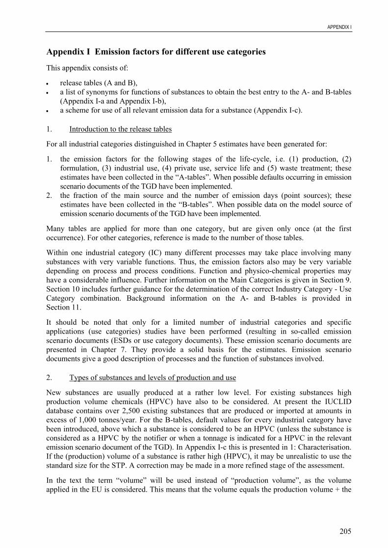
APPENDIX I
205
Appendix I Emission factors for different use categories
This appendix consists of:
• release tables (A and B),• a list of synonyms for functions of substances to obtain the best entry to the A- and B-tables
(Appendix I-a and Appendix I-b),• a scheme for use of all relevant emission data for a substance (Appendix I-c).
1. Introduction to the release tables
For all industrial categories distinguished in Chapter 5 estimates have been generated for:
1. the emission factors for the following stages of the life-cycle, i.e. (1) production, (2)formulation, (3) industrial use, (4) private use, service life and (5) waste treatment; theseestimates have been collected in the “A-tables”. When possible defaults occurring in emissionscenario documents of the TGD have been implemented.
2. the fraction of the main source and the number of emission days (point sources); theseestimates have been collected in the “B-tables”. When possible data on the model source ofemission scenario documents of the TGD have been implemented.
Many tables are applied for more than one category, but are given only once (at the firstoccurrence). For other categories, reference is made to the number of those tables.
Within one industrial category (IC) many different processes may take place involving manysubstances with very variable functions. Thus, the emission factors also may be very variabledepending on process and process conditions. Function and physico-chemical properties mayhave a considerable influence. Further information on the Main Categories is given in Section 9.Section 10 includes further guidance for the determination of the correct Industry Category - UseCategory combination. Background information on the A- and B-tables is provided inSection 11.
It should be noted that only for a limited number of industrial categories and specificapplications (use categories) studies have been performed (resulting in so-called emissionscenario documents (ESDs or use category documents). These emission scenario documents arepresented in Chapter 7. They provide a solid basis for the estimates. Emission scenariodocuments give a good description of processes and the function of substances involved.
2. Types of substances and levels of production and use
New substances are usually produced at a rather low level. For existing substances highproduction volume chemicals (HPVC) have also to be considered. At present the IUCLIDdatabase contains over 2,500 existing substances that are produced or imported at amounts inexcess of 1,000 tonnes/year. For the B-tables, default values for every industrial category havebeen introduced, above which a substance is considered to be an HPVC (unless the substance isconsidered as a HPVC by the notifier or when a tonnage is indicated for a HPVC in the relevantemission scenario document of the TGD). In Appendix I-c this is presented in 1: Characterisation.If the (production) volume of a substance is rather high (HPVC), it may be unrealistic to use thestandard size for the STP. A correction may be made in a more refined stage of the assessment.
In the text the term “volume” will be used instead of “production volume”, as the volumeapplied in the EU is considered. This means that the volume equals the production volume + the

APPENDIX I
206
volume imported in the EU - the volume exported from the EU (the substance as such, not thequantities imported in products). This is presented in Appendix I-c in 2: Tonnage.
A substance can have applications in more than one industrial category (IC) and/or use category(UC). As an assessment has to be made for all relevant applications of the substance, the input offractions for different industrial and use category combinations must be realised according to 3:Use and stages of the life-cycle in Appendix I-c.
3. Aspects of production
If specific data on emissions at production are known, these can be used instead of the tables(see Appendix I-c under 4: Production characteristics at “Specific emission information”). Alsofor the fraction of the main source specific data may be entered, either as the capacity(tonnes/day) or as the period (days/year) in which the substance is produced (see Appendix I-cunder 4: Production characteristics at “Production capacity”).
4. Aspects of formulation
For this stage of the life-cycle specific data may be entered on the fraction of the main sourceand the emissions/emission factors, see Appendix I-c under 5: Formulation characteristics. Forthe emissions, a refinement may be achieved by discriminating between cleaning with/withoutwater and soap. This has not been done yet.
In case a substance is applied in a formulation at a rather low level, unrealistic values for thefraction of the main source and the number of days will be derived from the tables using thetonnage as such. Therefore a correction should be made; a suggestion is to correct the tonnage asinput for the B-table in the following way. For example if the percentage of substance in theformulation is 0.1, the volume (tonnes/year) is multiplied by 100/0.1. This tonnage may then beused to estimate the fraction of the main source and the number of days using the tables. It ispossible to calculate an average in the case where a range of contents has been specified. Thishas been worked out in Appendix I-c in 5: Formulation characteristics at “Content in formulatedproduct”.
5. Aspects of industrial use
Industrial/professional use is referred to as “processing” in the A- and B-tables. Specific data onthe fraction of the main source and the emissions may be used as input (see Appendix I-c in 6:Processing characteristics). This will be repeated for every specified IC-UC combination. In casea specific scenario for an IC-UC combination exists, specific data will be asked.
6. Aspects of service life
The life cycle stage service life is only considered for articles produced in textile industry.
7. Aspects of private use
Specific data on the fraction of the main source and the emissions may be used (see Appendix I-c in 6: Private use characteristics). This will be possible for every specified IC-UC combinationfor which the stage of private use is relevant.

APPENDIX I
207
8. Aspects of waste treatment
Specific data on the fraction of the main source and the emissions may be used (see AppendixI-c in 6: Recovery characteristics). This will be possible for every specified IC-UC combinationfor which the stage of waste treatment is relevant. For waste treatment only situations where amaterial – which contains the chemical of interest – is recovered and processes to make it suitablefor re-use in its original application (recycling) or another application are taken into account.
9. Interpretation and use of the classification in “Main categories”
The main categories (MCs) were intended originally to provide a general impression of therelevance of the exposure during the whole life-cycle. The categorisation procedure outlined inChapter 5 allows for one entry of the Main category (MC) only, for all stages of the life-cycle.
In the context of environmental risk assessment Main Categories are often used to characteriserelease scenarios for the estimation of emissions to the environment at individual stages of thelife-cycle, i.e. at production, formulation and use. They can therefore be allocated to releasefractions, which are used as default values where specific information is lacking.
MC I “Use in closed systems”
This MC refers to the stage of production and industrial/professional use. At the stage ofproduction a substance should be assigned only to this category if it remains within a reactor oris transferred from vessel to vessel through closed pipework. The HEDSET distinguishesbetween three subcategories for intermediates.
For the stage of industrial/professional use this MC refers to substances that are used in closedsystems, e.g. the application of a substance in a transformer or the circulation circuit ofrefrigerators.
MC II “Use resulting in inclusion into or onto a matrix”
Use consisting of inclusion into or onto matrices means all processes where chemicals areincorporated into products or articles from which they (normally) will not be released into theenvironment. This is applicable to the stage of formulation, e.g., when a substance is included inthe emulsion layer of a photographic film. It also may refer to the stage of processing, e.g., whena paint additive ends up in the finished coating layer.
MC III “Non-dispersive use”
Non-dispersive use refers to chemicals which are used in such a way that only certain groups ofworkers, with knowledge of the process, come into contact with these chemicals. This meansthat the use of these chemicals is related to the number (and size) of the emission sources. So,this MC indicates industrial use at a limited number of sites (where emission reduction measuresmay be common practice).
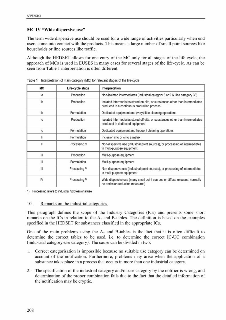
APPENDIX I
208
MC IV “Wide dispersive use”
The term wide dispersive use should be used for a wide range of activities particularly when endusers come into contact with the products. This means a large number of small point sources likehouseholds or line sources like traffic.
Although the HEDSET allows for one entry of the MC only for all stages of the life-cycle, theapproach of MCs is used in EUSES in many cases for several stages of the life-cycle. As can beseen from Table 1 interpretation is often different.
Table 1 Interpretation of main category (MC) for relevant stages of the life-cycle
MC Life-cycle stage Interpretation
Ia Production Non-isolated intermediates (Industrial category 3 or 9 & Use category 33)
Ib Production Isolated intermediates stored on-site, or substances other than intermediatesproduced in a continuous production process
Ib Formulation Dedicated equipment and (very) little cleaning operations
Ic Production Isolated intermediates stored off-site, or substances other than intermediatesproduced in dedicated equipment
Ic Formulation Dedicated equipment and frequent cleaning operations
II Formulation Inclusion into or onto a matrix
II Processing 1) Non-dispersive use (industrial point sources), or processing of intermediatesin multi-purpose equipment
III Production Multi-purpose equipment
III Formulation Multi-purpose equipment
III Processing 1) Non-dispersive use (industrial point sources), or processing of intermediatesin multi-purpose equipment
IV Processing 1) Wide dispersive use (many small point sources or diffuse releases; normallyno emission reduction measures)
1) Processing refers to industrial / professional use
10. Remarks on the industrial categories
This paragraph defines the scope of the Industry Categories (ICs) and presents some shortremarks on the ICs in relation to the A- and B-tables. The definition is based on the examplesspecified in the HEDSET for substances classified in the appropriate ICs.
One of the main problems using the A- and B-tables is the fact that it is often difficult todetermine the correct tables to be used, i.e. to determine the correct IC-UC combination(industrial category-use category). The cause can be divided in two:
1. Correct categorisation is impossible because no suitable use category can be determined onaccount of the notification. Furthermore, problems may arise when the application of asubstance takes place in a process that occurs in more than one industrial category.
2. The specification of the industrial category and/or use category by the notifier is wrong, anddetermination of the proper combination fails due to the fact that the detailed information ofthe notification may be cryptic.
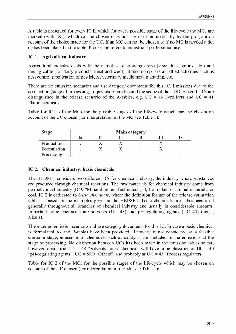
APPENDIX I
209
A table is presented for every IC in which for every possible stage of the life-cycle the MCs aremarked (with ‘X’), which can be chosen or which are used automatically by the program onaccount of the choice made for the UC. If an MC can not be chosen or if no MC is needed a dot(.) has been placed in the table. Processing refers to industrial / professional use.
IC 1. Agricultural industry
Agricultural industry deals with the activities of growing crops (vegetables, grains, etc.) andraising cattle (for dairy products, meat and wool). It also comprises all allied activities such aspest control (application of pesticides, veterinary medicines), manuring, etc.
There are no emission scenarios and use category documents for this IC. Emissions due to theapplication (stage of processing) of pesticides are beyond the scope of the TGD. Several UCs aredistinguished in the release scenario of the A-tables, e.g. UC = 19 Fertilisers and UC = 41Pharmaceuticals.
Table for IC 1 of the MCs for the possible stages of the life-cycle which may be chosen onaccount of the UC chosen (for interpretation of the MC see Table 1):
Stage Main categoryIa Ib Ic II III IV
Production . X X . X .Formulation . X X . X .Processing . . . . . .
IC 2. Chemical industry: basic chemicals
The HEDSET considers two different ICs for chemical industry, the industry where substancesare produced through chemical reactions. The raw materials for chemical industry come frompetrochemical industry (IC 9 “Mineral oil and fuel industry”), from plant or animal materials, orcoal. IC 2 is dedicated to basic chemicals, where the definition for use of the release estimationtables is based on the examples given in the HEDSET: basic chemicals are substances usedgenerally throughout all branches of chemical industry and usually in considerable amounts.Important basic chemicals are solvents (UC 48) and pH-regulating agents (UC 40) (acids,alkalis).
There are no emission scenario and use category documents for this IC. In case a basic chemicalis formulated A- and B-tables have been provided. Recovery is not considered as a feasibleemission stage; emissions of chemicals such as catalysts are included in the emissions at thestage of processing. No distinction between UCs has been made in the emission tables so far;however, apart from UC = 48 “Solvents” most chemicals will have to be classified as UC = 40“pH-regulating agents”, UC = 55/0 “Others”, and probably as UC = 43 “Process regulators”.
Table for IC 2 of the MCs for the possible stages of the life-cycle which may be chosen onaccount of the UC chosen (for interpretation of the MC see Table 1):

APPENDIX I
210
Stage Main categoryIa Ib Ic II III IV
Production . X X . X .Formulation . X X . X .Processing . . . . . .
IC 3. Chemical industry: chemicals used in synthesis
The definition for chemicals used in synthesis based on the examples given in the HEDSET is:chemicals used in synthesis are substances either regulating the chemical reaction process (e.g.catalysts) or being used as an intermediate (i.e. chemicals that are formed and can be isolated atan intermediate step between starting material and the final product in a sequence of chemicalprocesses). The HEDSET includes monomers in intermediates, which is only valid in the releaseestimation tables for the stage of production. For the processing stage the tables of IC 11“Polymers industry” are used (see also subparagraph 4.2.5).
Apart from UC = 33 “Intermediates” most chemicals in this IC will have to be classified as UC =43 “Process regulators” or UC = 55/0 “Others”. Formulation may be applicable for somechemicals, whilst recovery is unlikely.
Table for IC 3 of the MCs for the possible stages of the life-cycle which may be chosen onaccount of the UC chosen (for interpretation of the MC see Table 1):
Stage Main categoryIa Ib Ic II III IV
Production (UC ≠ 33)Production (UC = 33)
.X
XX
XX
.
.X.
.
.Formulation (UC ≠ 33) . X X . X .Processing . X X . X .
IC 4. Electrical/electronic industry
In electrical/electronic industry a wide range of products is manufactured. It comprises both themanufacture of components like resistors, transistors, capacitors, diodes, lamps, etc. and theproduction of televisions, radios, computers (PC’s as well as mainframes), radar installations,complete telephone exchanges, etc. In the manufacturing processes constituent processes maytake place. The main constituent processes are electroplating, polymer processing, and paintapplication. The emissions of substances used in these separate processes are not covered in IC4, but in the following ICs:
• IC 8. “Metal extraction, refining and processing industry”: electroplating and other metalprocessing (e.g. use of metalworking fluids);
• IC 11. “Polymers industry”: polymer processing (shaping of thermoplastics and curing ofprepolymers e.g. for the embedding of electronic components);
• IC 14. “Paints, lacquers and varnishes industry”: application of coating products by allmeans of methods like spraying, curtain coating, etc.
There are no emission scenario and use category documents for IC 4. There are many differentapplications, however, in this IC, which may be characteristic and specific for it, e.g., the
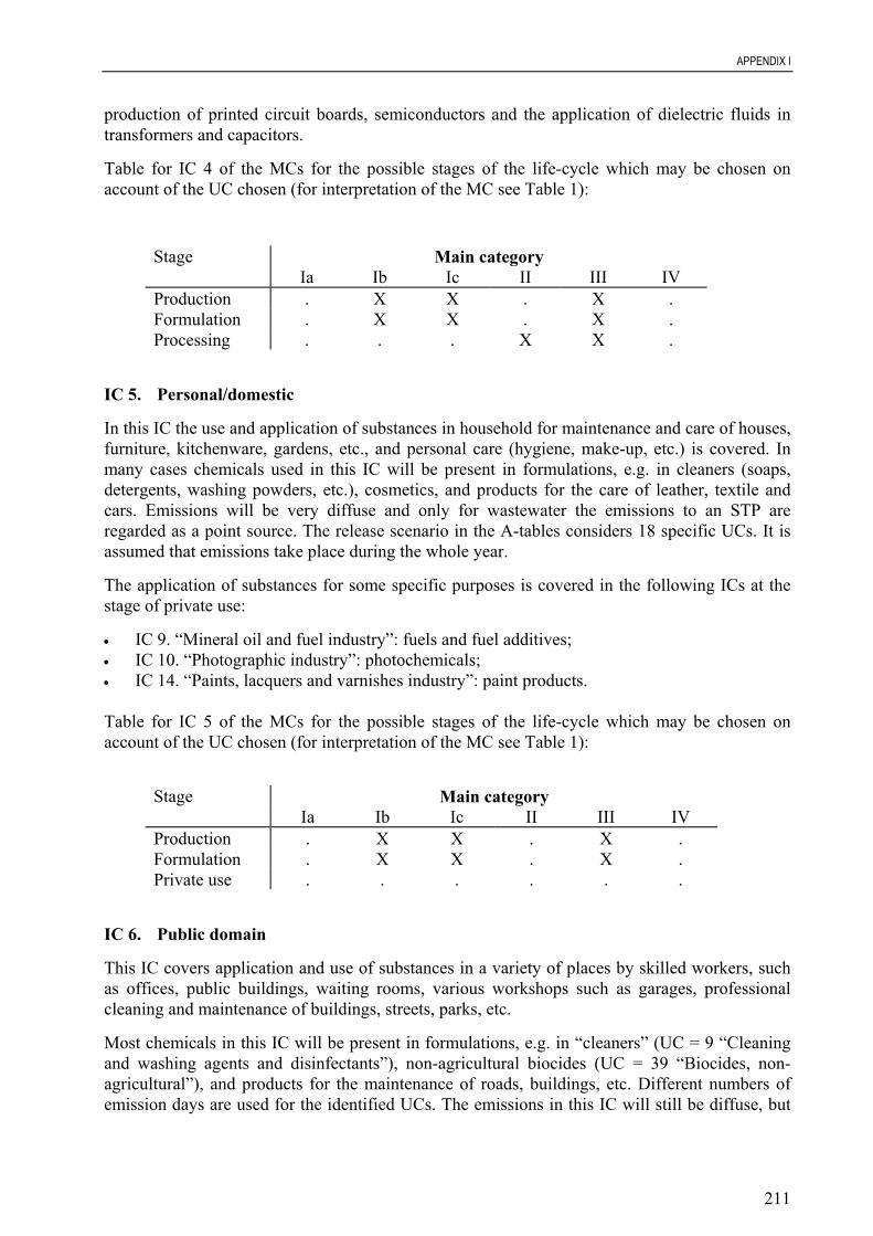
APPENDIX I
211
production of printed circuit boards, semiconductors and the application of dielectric fluids intransformers and capacitors.
Table for IC 4 of the MCs for the possible stages of the life-cycle which may be chosen onaccount of the UC chosen (for interpretation of the MC see Table 1):
Stage Main categoryIa Ib Ic II III IV
Production . X X . X .Formulation . X X . X .Processing . . . X X .
IC 5. Personal/domestic
In this IC the use and application of substances in household for maintenance and care of houses,furniture, kitchenware, gardens, etc., and personal care (hygiene, make-up, etc.) is covered. Inmany cases chemicals used in this IC will be present in formulations, e.g. in cleaners (soaps,detergents, washing powders, etc.), cosmetics, and products for the care of leather, textile andcars. Emissions will be very diffuse and only for wastewater the emissions to an STP areregarded as a point source. The release scenario in the A-tables considers 18 specific UCs. It isassumed that emissions take place during the whole year.
The application of substances for some specific purposes is covered in the following ICs at thestage of private use:
• IC 9. “Mineral oil and fuel industry”: fuels and fuel additives;• IC 10. “Photographic industry”: photochemicals;• IC 14. “Paints, lacquers and varnishes industry”: paint products.
Table for IC 5 of the MCs for the possible stages of the life-cycle which may be chosen onaccount of the UC chosen (for interpretation of the MC see Table 1):
Stage Main categoryIa Ib Ic II III IV
Production . X X . X .Formulation . X X . X .Private use . . . . . .
IC 6. Public domain
This IC covers application and use of substances in a variety of places by skilled workers, suchas offices, public buildings, waiting rooms, various workshops such as garages, professionalcleaning and maintenance of buildings, streets, parks, etc.
Most chemicals in this IC will be present in formulations, e.g. in “cleaners” (UC = 9 “Cleaningand washing agents and disinfectants”), non-agricultural biocides (UC = 39 “Biocides, non-agricultural”), and products for the maintenance of roads, buildings, etc. Different numbers ofemission days are used for the identified UCs. The emissions in this IC will still be diffuse, but
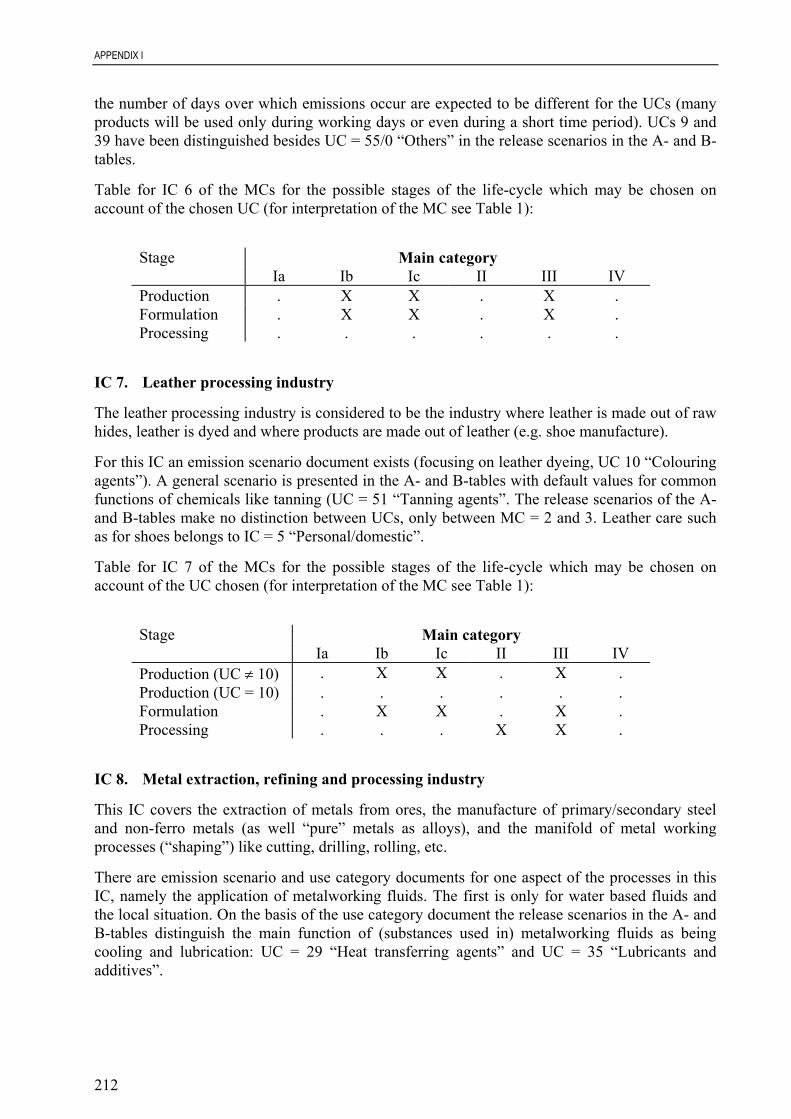
APPENDIX I
212
the number of days over which emissions occur are expected to be different for the UCs (manyproducts will be used only during working days or even during a short time period). UCs 9 and39 have been distinguished besides UC = 55/0 “Others” in the release scenarios in the A- and B-tables.
Table for IC 6 of the MCs for the possible stages of the life-cycle which may be chosen onaccount of the chosen UC (for interpretation of the MC see Table 1):
Stage Main categoryIa Ib Ic II III IV
Production . X X . X .Formulation . X X . X .Processing . . . . . .
IC 7. Leather processing industry
The leather processing industry is considered to be the industry where leather is made out of rawhides, leather is dyed and where products are made out of leather (e.g. shoe manufacture).
For this IC an emission scenario document exists (focusing on leather dyeing, UC 10 “Colouringagents”). A general scenario is presented in the A- and B-tables with default values for commonfunctions of chemicals like tanning (UC = 51 “Tanning agents”. The release scenarios of the A-and B-tables make no distinction between UCs, only between MC = 2 and 3. Leather care suchas for shoes belongs to IC = 5 “Personal/domestic”.
Table for IC 7 of the MCs for the possible stages of the life-cycle which may be chosen onaccount of the UC chosen (for interpretation of the MC see Table 1):
Stage Main categoryIa Ib Ic II III IV
Production (UC ≠ 10) . X X . X .Production (UC = 10) . . . . . .Formulation . X X . X .Processing . . . X X .
IC 8. Metal extraction, refining and processing industry
This IC covers the extraction of metals from ores, the manufacture of primary/secondary steeland non-ferro metals (as well “pure” metals as alloys), and the manifold of metal workingprocesses (“shaping”) like cutting, drilling, rolling, etc.
There are emission scenario and use category documents for one aspect of the processes in thisIC, namely the application of metalworking fluids. The first is only for water based fluids andthe local situation. On the basis of the use category document the release scenarios in the A- andB-tables distinguish the main function of (substances used in) metalworking fluids as beingcooling and lubrication: UC = 29 “Heat transferring agents” and UC = 35 “Lubricants andadditives”.
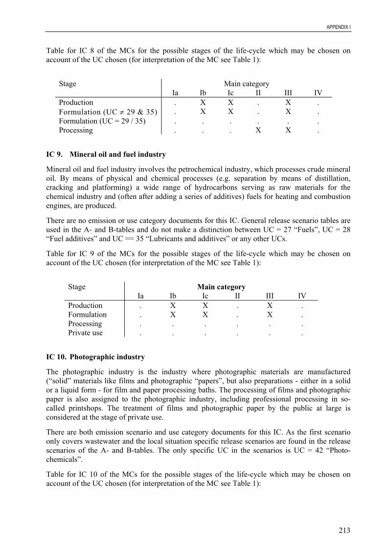
APPENDIX I
213
Table for IC 8 of the MCs for the possible stages of the life-cycle which may be chosen onaccount of the UC chosen (for interpretation of the MC see Table 1):
Stage Main categoryIa Ib Ic II III IV
Production . X X . X .Formulation (UC ≠ 29 & 35) . X X . X .Formulation (UC = 29 / 35) . . . . . .Processing . . . X X .
IC 9. Mineral oil and fuel industry
Mineral oil and fuel industry involves the petrochemical industry, which processes crude mineraloil. By means of physical and chemical processes (e.g. separation by means of distillation,cracking and platforming) a wide range of hydrocarbons serving as raw materials for thechemical industry and (often after adding a series of additives) fuels for heating and combustionengines, are produced.
There are no emission or use category documents for this IC. General release scenario tables areused in the A- and B-tables and do not make a distinction between UC = 27 “Fuels”, UC = 28“Fuel additives” and UC == 35 “Lubricants and additives” or any other UCs.
Table for IC 9 of the MCs for the possible stages of the life-cycle which may be chosen onaccount of the UC chosen (for interpretation of the MC see Table 1):
Stage Main categoryIa Ib Ic II III IV
Production . X X . X .Formulation . X X . X .Processing . . . . . .Private use . . . . . .
IC 10. Photographic industry
The photographic industry is the industry where photographic materials are manufactured(“solid” materials like films and photographic “papers”, but also preparations - either in a solidor a liquid form - for film and paper processing baths. The processing of films and photographicpaper is also assigned to the photographic industry, including professional processing in so-called printshops. The treatment of films and photographic paper by the public at large isconsidered at the stage of private use.
There are both emission scenario and use category documents for this IC. As the first scenarioonly covers wastewater and the local situation specific release scenarios are found in the releasescenarios of the A- and B-tables. The only specific UC in the scenarios is UC = 42 “Photo-chemicals”.
Table for IC 10 of the MCs for the possible stages of the life-cycle which may be chosen onaccount of the UC chosen (for interpretation of the MC see Table 1):
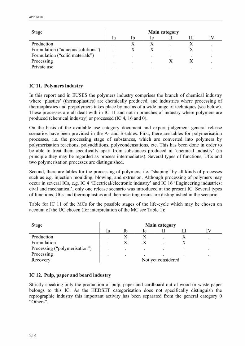
APPENDIX I
214
Stage Main categoryIa Ib Ic II III IV
Production . X X . X .Formulation (“aqueous solutions”) . X X . X .Formulation (“solid materials”) . . . . . .Processing . . . X X .Private use . . . . . .
IC 11. Polymers industry
In this report and in EUSES the polymers industry comprises the branch of chemical industrywhere ‘plastics’ (thermoplastics) are chemically produced, and industries where processing ofthermoplastics and prepolymers takes place by means of a wide range of techniques (see below).These processes are all dealt with in IC 11 and not in branches of industry where polymers areproduced (chemical industry) or processed (IC 4, 16 and 0).
On the basis of the available use category document and expert judgement general releasescenarios have been provided in the A- and B-tables. First, there are tables for polymerisationprocesses, i.e. the processing stage of substances, which are converted into polymers bypolymerisation reactions, polyadditions, polycondensations, etc. This has been done in order tobe able to treat them specifically apart from substances produced in ‘chemical industry’ (inprinciple they may be regarded as process intermediates). Several types of functions, UCs andtwo polymerisation processes are distinguished.
Second, there are tables for the processing of polymers, i.e. “shaping” by all kinds of processessuch as e.g. injection moulding, blowing, and extrusion. Although processing of polymers mayoccur in several ICs, e.g. IC 4 ‘Electrical/electronic industry’ and IC 16 ‘Engineering industries:civil and mechanical’, only one release scenario was introduced at the present IC. Several typesof functions, UCs and thermoplastics and thermosetting resins are distinguished in the scenario.
Table for IC 11 of the MCs for the possible stages of the life-cycle which may be chosen onaccount of the UC chosen (for interpretation of the MC see Table 1):
Stage Main categoryIa Ib Ic II III IV
Production . X X . X .Formulation . X X . X .Processing (“polymerisation”) . . . . . .Processing . . . . . .Recovery Not yet considered
IC 12. Pulp, paper and board industry
Strictly speaking only the production of pulp, paper and cardboard out of wood or waste paperbelongs to this IC. As the HEDSET categorisation does not specifically distinguish thereprographic industry this important activity has been separated from the general category 0“Others”.

APPENDIX I
215
For this IC both emission scenario and use category documents are available. The emissionscenario document deals with wastewater and the local situation. The release scenarios in the A-and B-tables are applicable to the stage of processing printing and allied processes, and theproduction of pulp, paper and board (including paper dyeing). The stage of recovery (paperrecycling) is also considered in the tables.
Two UCs are specifically considered, i.e. UC 10 “Colouring agents” used as pigments in inksand as dyes for paper mass colouring, UC 20 and 31 (“Fillers” and “Impregnation agents”) bothused in paper production and UC 45 “Reprographic agents” which is a “collection” of all kindsof uses and functions of substances in printing and allied processes.
Table for IC 12 of the MCs for the possible stages of the life-cycle which may be chosen onaccount of the UC chosen (for interpretation of the MC see Table 1):
Stage Main categoryIa Ib Ic II III IV
Production (UC ≠ 10) . X X . X .Production (UC = 10) . . . . . .Formulation . X X . X .Recovery . . . . . .
IC 13. Textile processing industry
This IC covers treatment of fibres (“cleaning”, spinning, dyeing, etc.), weaving, and finishing(e.g. impregnation, coating, etc.).
For this IC both emission scenario and use category documents are available. The releasescenarios in the A- and B-tables are specific for IC 10 “Colouring agents” and general for otherrelevant UCs.
Table for IC 13 of the MCs for the possible stages of the life-cycle which may be chosen onaccount of the UC chosen (for interpretation of the MC see Table 1):
Stage Main categoryIa Ib Ic II III IV
Production (UC ≠ 10) . X X . X .Production (UC = 10) . . . . . .Formulation . X X . X .Processing . . . . . .Private use (only UC = 10) . . . . . .
IC 14. Paints, lacquers and varnishes industry
Apart from the manufacture of coating products (stage of formulation) such as paints this reportand EUSES also consider application of these products as belonging to this IC. This has beendone because otherwise many release scenarios would have to be introduced in many other ICs.These could include for example IC 5 “Personal/domestic” for private use, IC 6 “Public domain”for professional application by house painters and in (small) workshops, and many industrialapplications. The latter could include IC 16 “Engineering industries: civil and mechanical” in the

APPENDIX I
216
manufacturing of motor cars, constructions, etc. and IC 8 “Metal extraction, refining andprocessing industry”.
There is an emission scenario on paint manufacture and application (stages of formulation andprocessing respectively) and a use category document for paint manufacture. The A- and B-tables have release scenarios for both water-based and solvent-based coatings systems anddistinguish 8 specific UCs; both industrial use (stage of processing) and private use. The stage offormulation concerns the manufacture of the coating products.
Table for IC 14 of the MCs for the possible stages of the life-cycle which may be chosen onaccount of the UC chosen (for interpretation of the MC see Table 1):
Stage Main categoryIa Ib Ic II III IV
Production . X X . X .Formulation . X X . X .Processing . . . . . .Private use . . . . . .
IC 15. Engineering industries: civil and mechanical
Industrial activities belonging to this IC include wood processing industries (e.g. woodenfurniture), motor car manufacture, building industry, etc. There are no emission or use categorydocuments for this IC. Processes such as coating application take place in many of theseactivities; these processes are dealt with in the IC where the specific process belongs (coatingapplication: IC 14 “Paints, lacquers and varnishes industry”). For the present IC the samegeneral release scenarios as for IC 15 “Others” are used in the A- and B-tables.
Table for IC 15 of the MCs for the possible stages of the life-cycle which may be chosen onaccount of the UC chosen (for interpretation of the MC see Table 1):
Stage Main categoryIa Ib Ic II III IV
Production . X X . X .Formulation . X X . X .Processing . . . X X X
IC 16. Others
All processes and activities, which can not be placed in one of the previous ICs, belong to this IC.An example is the food processing industry. General release scenarios are used in the A- and B-tables.
Table for IC 16 of the MCs for the possible stages of the life-cycle which may be chosen onaccount of the UC chosen (for interpretation of the MC see Table 1):

APPENDIX I
217
Stage Main categoryIa Ib Ic II III IV
Production . X X . X .Formulation . X X . X .Processing . . . X X X
11. Relationship between industrial categories
In practice all chemicals originate from IC 2 & 3 “Chemical industry” and go from there to oneof the other ICs (or remain in chemical industry). Substances such as monomers, cross-linkingagents, and curing agents take a special position. These substances are basic chemicals (rawmaterials) for IC 11 “Polymers industry” for the production of polymers by polymerisationreactions and other reactions like polyaddition and polycondensation. Despite the fact that thismay be seen as the stage of production in IC 3 (UC 33 “Intermediates”) they have beenintroduced in the emission tables of IC 11 “Polymers industry” as UC 43 “Process regulators”.Besides the production of polymers this IC also deals with the processing of the polymers(thermoplastics) and prepolymers (prepolymers are macromolecular substances such as polyesterand epoxy resins which are transformed in thermosetting resins with the aid of curing agents,such as initiators - mainly organic peroxides - and cross-linking agents - mainly the monomerstyrene - for polyesters, and curing agents like amines for epoxy resins). The processing stage of(pre) polymers involves the manufacture of all kind of articles and parts of objects from the basicmaterials.
The releases in both IC 5 “Personal/domestic” and IC 6 “Public domain” have a diffuse character.In IC 5 the use of chemicals in households is covered and in IC 6 the use in offices, publicbuildings, parks, railway stations, in the street, etc. The main differences will be found in theamounts (e.g. because of the size of the building) and the number of days that emissions occur.
12. History of the A- and B-tables
In the development of the quantitative risk assessment system for new substances DRANC(Dutch Risk Assessment System for New Chemicals) (Toet et al., 1991; Vermeire et al., 1992)emission tables were developed for a limited number of applications. The applications consideredwere textile dyes, photo-chemicals, metalworking fluids, hydraulic fluids, paper-chemicals, andintermediates. For these applications so-called use category documents were available. Nearly atthe same time PRISEC (PRIority Setting system for Existing Chemicals) was developed (Van deMeent and Toet, 1992). For this system emission tables were developed for the 15 industrialcategories distinguished at that time in the HEDSET (EC/OECD Harmonised Electronic DataSet). The emission factors were established by means of expert judgement and tended to theworst-case situation. For the local release estimation tables were supplied containing expertjudgement for the order of magnitude of the daily amount of the substances for every relevantstage of the life-cycle on the basis of the tonnage. The ranges of the tonnages were typical forsubstances produced in limited amounts. When the TGD and EUSES were developed thesetables were transformed into what are now referred to as the A- and B-tables (A-tables withemission factors and B-tables with size of the operation information) and extended in thefollowing way:

APPENDIX I
218
1. extension of the tables with emission factors for several industrial categories. This may befor example for the introduction of main categories or specific use categories. This was alsoachieved by expert judgement trying to obtain realistic worst-case estimates;
2. insertion of the emission factors of the use category documents mentioned before in theappropriate industrial categories;
3. introduction of B-tables in order to cover higher tonnages for HPVCs (High ProductionVolume Chemicals). This was also done by expert judgement;
4. new A- and B-tables were developed for the new industrial category 16 ‘Engineeringindustries’.
The final tables were discussed and endorsed in a special EU Expert Meeting on Releaseestimation (Sept. 1995) that was held in the context of the development of the TGD.Subsequently, the tables were introduced in the TGD and EUSES.
13. Calculating releases per stage of the life-cycle
Using the fractions released from the A-tables, the total amount released (per stage of thelife-cycle and for each environmental compartment) can be calculated with the followingequations. For each stage (except for production) the losses in the previous stage are takeninto account.
The fractions released in each stage of the life-cycle and to every compartment are denotedby Fi,j where i is the stage in the life-cycle and j is the compartment:
i stage of the life-cycle j compartment
1 production a air2 formulation w water3 processing s soil4 private use5 recovery
Industrial/professional use is indicated as “processing” in the A- and B-tables. Service life is notincluded as a separate stage of the life-cycle. With respect to waste disposal, only recovery isaddressed in the A- and B-tables.
The release per stage of the life-cycle (in tonnes per year) can be calculated by:
1.
Production RELEASE1,j air F1, a • PRODVOLwater F1, w • PRODVOLsoil F1, s • PRODVOLtotal ΣF1, j • PRODVOL
amount used: TONNAGE
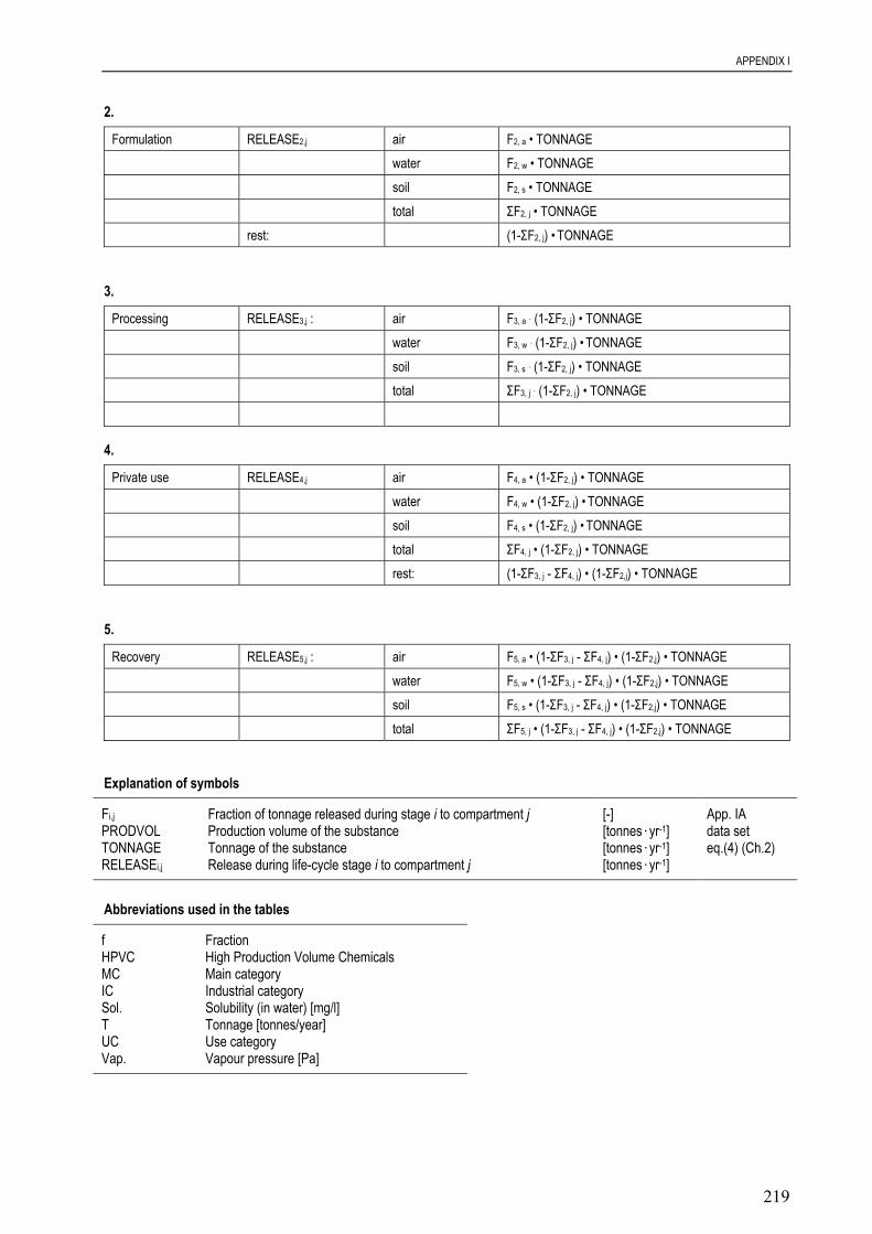
APPENDIX I
219
2.
Formulation RELEASE2,j air F2, a • TONNAGEwater F2, w • TONNAGEsoil F2, s • TONNAGEtotal ΣF2, j • TONNAGE
rest: (1-ΣF2, j) • TONNAGE
3.
Processing RELEASE3,j : air F3, a . (1-ΣF2, j) • TONNAGEwater F3, w . (1-ΣF2, j) • TONNAGEsoil F3, s . (1-ΣF2, j) • TONNAGEtotal ΣF3, j . (1-ΣF2, j) • TONNAGE
4.
Private use RELEASE4,j air F4, a • (1-ΣF2, j) • TONNAGEwater F4, w • (1-ΣF2, j) • TONNAGEsoil F4, s • (1-ΣF2, j) • TONNAGEtotal ΣF4, j • (1-ΣF2, j) • TONNAGErest: (1-ΣF3, j - ΣF4, j) • (1-ΣF2,j) • TONNAGE
5.
Recovery RELEASE5,j : air F5, a • (1-ΣF3, j - ΣF4, j) • (1-ΣF2,j) • TONNAGEwater F5, w • (1-ΣF3, j - ΣF4, j) • (1-ΣF2,j) • TONNAGEsoil F5, s • (1-ΣF3, j - ΣF4, j) • (1-ΣF2,j) • TONNAGEtotal ΣF5, j • (1-ΣF3, j - ΣF4, j) • (1-ΣF2,j) • TONNAGE
Explanation of symbols
Fi,j Fraction of tonnage released during stage i to compartment j [-] App. IAPRODVOL Production volume of the substance [tonnes.yr-1] data set TONNAGE Tonnage of the substance [tonnes.yr-1] eq.(4) (Ch.2)RELEASEi,j Release during life-cycle stage i to compartment j [tonnes.yr-1]
Abbreviations used in the tables
f FractionHPVC High Production Volume ChemicalsMC Main categoryIC Industrial categorySol. Solubility (in water) [mg/l]T Tonnage [tonnes/year]UC Use categoryVap. Vapour pressure [Pa]

APPENDIX I
220
A-tables
Estimates for the emission factors (fractions released)

APPENDIX I
221
IC = 1: AGRICULTURAL INDUSTRY
PRODUCTION Table A1.1
Compartment Conditions Emission factorsSol. (mg/l) Vap. (Pa) All MC's MC=1b MC=1c MC=3 1)
Air <1 0 0 0.000011-10 0 0.00001 0.000110-100 0.00001 0.0001 0.001100-1000 0.0001 0.001 0.01000-10,000 0.001 0.005 0.05≥10,000 0.005 0.01 0.05
T (tonnes/year)
Wastewater <1000 0.02≥1,000 0.003
Soil 0.0001
1) Default
FORMULATION Table A2.1
Compartment Conditions Emission factorsSol. (mg/l) Vap. (Pa) All MC's MC=1b MC=1c MC=3 1)
Air <10 0.0005 0.001 0.002510-100 0.001 0.0025 0.005100-1,000 0.0025 0.005 0.01≥1,000 0.005 0.01 0.025
T (tonnes/year)
Wastewater <1,000 0.02≥1,000 0.003
Soil 0.0001
1) Default
INDUSTRIAL USE Table A3.1 *
UC's Description Emission factors to: Air Surface water SoilDefault 0.1 0.1 0.83 areosol propellants 1 0 09, 10, 36 cleaning/washing agents and additives 0 0.1 0.4
+ colorants + odour agents19 fertilisers 0 0.05 0.9526 food/feedstuff additives 0 0 0.0538, 50 pesticides + surfactants 0.05 0.1 0.8541 pharmaceuticals (external application) 0 0 0.141 pharmaceuticals (internal application) 0 0 048 solvents 1 0 0
* Fertilisers and pesticides + surfactants go to agricultural soil on the regional and continental scale, the others go to industrial soil

APPENDIX I
222
PRIVATE USE Not applicable
WASTE TREATMENT Not applicable
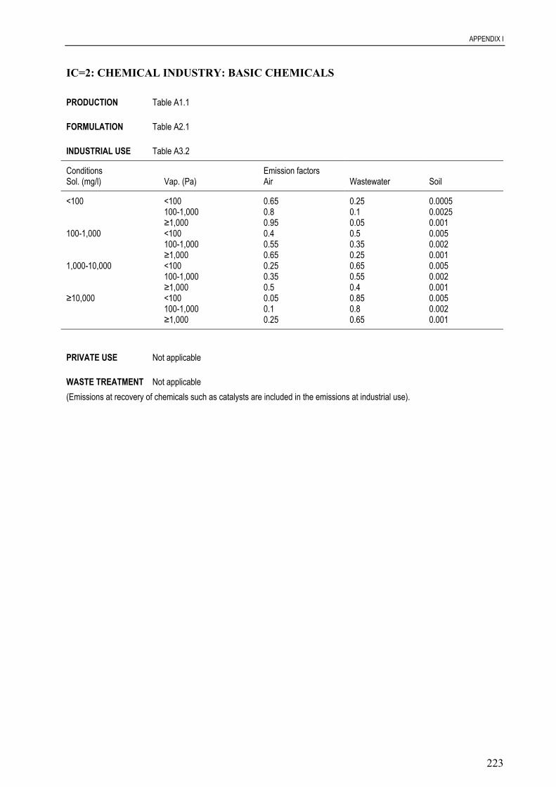
APPENDIX I
223
IC=2: CHEMICAL INDUSTRY: BASIC CHEMICALS
PRODUCTION Table A1.1
FORMULATION Table A2.1
INDUSTRIAL USE Table A3.2
Conditions Emission factorsSol. (mg/l) Vap. (Pa) Air Wastewater Soil
<100 <100 0.65 0.25 0.0005100-1,000 0.8 0.1 0.0025≥1,000 0.95 0.05 0.001
100-1,000 <100 0.4 0.5 0.005100-1,000 0.55 0.35 0.002≥1,000 0.65 0.25 0.001
1,000-10,000 <100 0.25 0.65 0.005100-1,000 0.35 0.55 0.002≥1,000 0.5 0.4 0.001
≥10,000 <100 0.05 0.85 0.005100-1,000 0.1 0.8 0.002≥1,000 0.25 0.65 0.001
PRIVATE USE Not applicable
WASTE TREATMENT Not applicable(Emissions at recovery of chemicals such as catalysts are included in the emissions at industrial use).

APPENDIX I
224
IC = 3: CHEMICAL INDUSTRY: CHEMICALS USED IN SYNTHESIS
PRODUCTION Table A1.1 for UC ≠ 33 (intermediates)Table A1.2 for UC = 33 (intermediates)
Compartment Conditions Emission factorsSol. (mg/l) Vap. (Pa) All MC's MC=1a MC=1b MC=1c
Air <1 0 0 01-10 0 0 0.0000110-100 0 0.00001 0.0001100-1,000 0.00001 0.0001 0.0011,000-10,000 0.0001 0.001 0.01≥10,000 0.001 0.01 0.025
Process T (tonnes/year)Wastewater Wet <1,000 0.02
≥1,000 0.003Dry 0
Soil 0 0.00001 0.0001
FORMULATION Table A2.1
INDUSTRIAL USE Table A3.3
Compartment Conditions Emission factorsSol. (mg/l) Vap. (Pa) All MC's MC = 1b MC = 1c MC = 3 (1)
Air <1 0 0 0.000011-10 0 0 0.000110-100 0 0.00001 0.001100-1,000 0.00001 0.0001 0.011,000-10,000 0.0001 0.001 0.025≥10,000 0.001 0.005 0.05
Process T (tonnes/year)Wastewater Wet <1,000 0.02
≥1,000 0.007 0.0005Dry 0
Soil 0.0001
1) DefaultRemark: The releases at industrial use for use category 33 (intermediates) should be added to the releases at production unless the notifierstates that the substance is processed elsewhere.
PRIVATE USE Not applicable
WASTE TREATMENT Not applicable
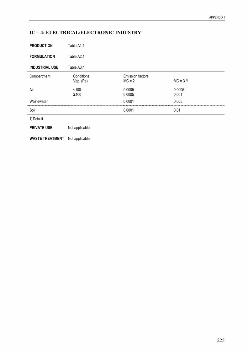
APPENDIX I
225
IC = 4: ELECTRICAL/ELECTRONIC INDUSTRY
PRODUCTION Table A1.1
FORMULATION Table A2.1
INDUSTRIAL USE Table A3.4
Compartment Conditions Emission factorsVap. (Pa) MC = 2 MC = 3 1)
Air <100 0.0005 0.0005≥100 0.0005 0.001
Wastewater 0.0001 0.005
Soil 0.0001 0.01
1) Default
PRIVATE USE Not applicable
WASTE TREATMENT Not applicable

APPENDIX I
226
IC = 5: PERSONAL /DOMESTIC
PRODUCTION Table A1.1 for UC ≠ 9 (cleaning/washing agents) and 15 (cosmetics)A1# for UC = 9 and 15 (if production volume < 1,000 tonnes/year Table A1.1 applies)
Compartment Conditions Emission factorsSol. (mg/l) Vap. (Pa) Batch process 1) Continuous process 2)
Air 0.000 001 0.000 001Wastewater 3) 4)
Solid waste 0 0
1) e.g., ethoxilation to nonionic surfactants and production of amphoteric and cationic surfactants2) e.g., sulphonation and sulphation to anionic surfactants3) According to the emission scenario document < 0.3 % (worst case = 0.003)4) According to the emission scenario document < 0.1 % (worst case = 0.001)
FORMULATION Table A2.1 for UC ≠ 9 (cleaning/washing agents) and 15 (cosmetics)Table A2# for UC = 9 (cleaning/washing agents) and UC15 (cosmetics)
Compartment Conditions Emission factorsSol. (mg/l) Vap. (Pa) Regular powder Compact powder Liquid Unknown
Air 0.000 2 0.000 2 0.000 02 0.000 2Wastewater 0.000 1 0.000 01 0.000 9 0.000 9Solid waste 0.007 3 0.008 1 0.003 2 0.008 1
INDUSTRIAL USE Not applicable
PRIVATE USE Table A4.1
Compartment Conditions Emission factorsUse category Sol. (mg/l) Vap. (Pa)
Air 2, 7, 8, 9, 10, 11, 15,41, 47, 50 03 15 0.000526 <5,000 0
≥5,000 0.01
35 <5,000 0≥5,000 0.05
36 <100 0.05100-2,500 0.22,500-10,000 0.5≥10,000 0.9
38 (herbicides) 0.01(pesticides, garden) 0.05(pesticides, pets) <100 0.05
100-5,000 0.1≥5,000 0.8
Table A4.1 continued overleaf
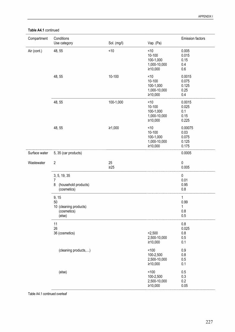
APPENDIX I
227
Table A4.1 continued
Compartment Conditions Emission factorsUse category Sol. (mg/l) Vap. (Pa)
Air (cont.) 48, 55 <10 <10 0.00510-100 0.015100-1,000 0.151,000-10,000 0.4≥10,000 0.6
48, 55 10-100 <10 0.001510-100 0.075100-1,000 0.1251,000-10,000 0.25≥10,000 0.4
48, 55 100-1,000 <10 0.001510-100 0.025100-1,000 0.11,000-10,000 0.15≥10,000 0.225
48, 55 ≥1,000 <10 0.0007510-100 0.03100-1,000 0.0751,000-10,000 0.125≥10,000 0.175
Surface water 5, 35 (car products) 0.0005
Wastewater 2 25 0≥25 0.005
3, 5, 19, 35 07 0.018 (household products) 0.95
(cosmetics) 0.8
9, 15 150 0.9910 (cleaning products) 1
(cosmetics) 0.8(else) 0.5
11 0.826 0.02536 (cosmetics) <2,500 0.8
2,500-10,000 0.5≥10,000 0.1
(cleaning products,…) <100 0.9100-2,500 0.82,500-10,000 0.5≥10,000 0.1
(else) <100 0.5100-2,500 0.32,500-10,000 0.2≥10,000 0.05
Table A4.1 continued overleaf
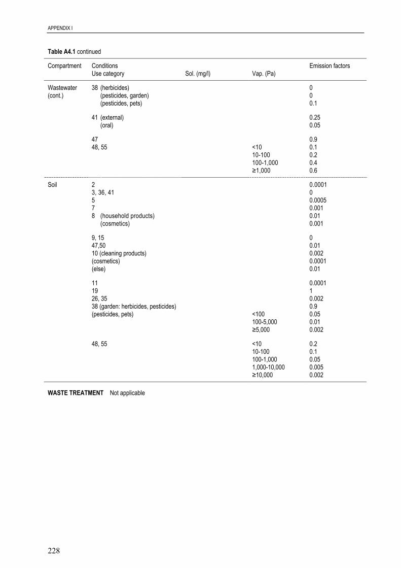
APPENDIX I
228
Table A4.1 continued
Compartment Conditions Emission factorsUse category Sol. (mg/l) Vap. (Pa)
Wastewater 38 (herbicides) 0(cont.) (pesticides, garden) 0
(pesticides, pets) 0.1
41 (external) 0.25(oral) 0.05
47 0.948, 55 <10 0.1
10-100 0.2100-1,000 0.4≥1,000 0.6
Soil 2 0.00013, 36, 41 05 0.00057 0.0018 (household products) 0.01
(cosmetics) 0.001
9, 15 047,50 0.0110 (cleaning products) 0.002(cosmetics) 0.0001(else) 0.01
11 0.000119 126, 35 0.00238 (garden: herbicides, pesticides) 0.9(pesticides, pets) <100 0.05
100-5,000 0.01≥5,000 0.002
48, 55 <10 0.210-100 0.1100-1,000 0.051,000-10,000 0.005≥10,000 0.002
WASTE TREATMENT Not applicable
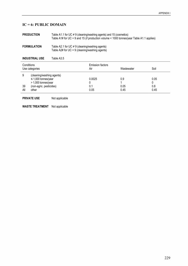
APPENDIX I
229
IC = 6: PUBLIC DOMAIN
PRODUCTION Table A1.1 for UC ≠ 9 (cleaning/washing agents) and 15 (cosmetics)Table A1# for UC = 9 and 15 (if production volume < 1000 tonnes/year Table A1.1 applies)
FORMULATION Table A2.1 for UC ≠ 9 (cleaning/washing agents)Table A2# for UC = 9 (cleaning/washing agents)
INDUSTRIAL USE Table A3.5
Conditions Emission factorsUse categories Air Wastewater Soil
9 (cleaning/washing agents)≤ 1,000 tonnes/year 0.0025 0.9 0.05> 1,000 tonnes/year 0 1 0
39 (non-agric. pesticides) 0.1 0.05 0.8All other 0.05 0.45 0.45
PRIVATE USE Not applicable
WASTE TREATMENT Not applicable

APPENDIX I
230
IC = 7: LEATHER PROCESSING INDUSTRY
PRODUCTION Table A1.1 for UC ≠10 (colorants)Table A1.3 for UC = 10 (colorants)
UC = 10 (Colorants)Compartment Conditions Emission factors
Sol. (mg/l)Air 0.0008Wastewater <2,000 0.015
2,000-10,000 0.0210,000-100,000 0.03100,000-500,000 0.05≥500,000 0.06
Soil 0.0001
FORMULATION Table A2.1
INDUSTRIAL USE Table A3.6
Compartment Conditions Emission factorsSol. (mg/l) Vap. (Pa) All MC's MC = 2 MC = 3 1)
Air <100 <100 0.001<100 ≥100 0.01≥100 0
Wastewater <100 0.05 0.9100-1,000 0.15 0.99≥1,000 0.25 0.99
Soil 0.01
1) Default
PRIVATE USE Not applicable
WASTE TREATMENT Not applicable

APPENDIX I
231
IC = 8: METAL EXTRACTION, REFINING AND PROCESSING INDUSTRY
PRODUCTION Table A1.1
FORMULATION Table A2.1 for UC ≠ 29 & 35Table A2.2 for UC = 29 & 35
Compartment Conditions Emission factorsVap. (Pa)
Air <1 0.000051-10 0.0000110-100 0.0005100-1,000 0.0025≥1,000 0.025
Wastewater 0.002Soil 0.00001
INDUSTRIAL USE Table A3.7
Compartment Conditions Emission factorsUC≠29&35Sol. (mg/l) MC = 2 MC = 3 1)
Air 0 0.25Wastewater <100 0.05 0.5
100-1,000 0.1 0.5≥1,000 0.25 0.5
Soil 0 0.05
Compartment Conditions Emission factorsUC=29&35log Henry
Air <2 0.0002≥2 0.002
Wastewater Pure oils 0.185Water based + unknown 0.316
Soil 0.0001
1) DefaultUC 29 = heat transferring agents, UC 35 = lubricants and additives; both are used in metalworking fluids
PRIVATE USE Not applicable
WASTE TREATMENT Not applicable

APPENDIX I
232
IC = 9: MINERAL OIL AND FUEL INDUSTRY
PRODUCTION Table A1.1
FORMULATION Table A2.1
INDUSTRIAL USE Table A3.8
CompartmenT Conditions Emission factorsVap. (Pa)
Air <1 0.00011-10 0.000510-100 0.001100-1,000 0.005≥1,000 0.01
Wastewater 0.0005
Soil 0.001
PRIVATE USE Table A4.2
Compartment Conditions Emission factorsVap. (Pa)
Air <10 0.00510-100 0.015100-1,000 0.151,000-10,000 0.4≥10,000 0.6
Wastewater 0.0005
Surface water 0.0001
Soil 0.0001
WASTE TREATMENT Not applicable

APPENDIX I
233
IC = 10: PHOTOGRAPHIC INDUSTRY
PRODUCTION Table A1.1
FORMULATION Table A2.1 default for formulations to be used in photographic baths (aqueous solutions)Table A2.3 for UC=42, and other UC's in the manufacture of solid materials
Compartment Conditions Emission factorsVap. (Pa)
Air <1 0.00011-10 0.00110-100 0.3100-1,000 0.7≥1,000 1
Wastewater Control of crystal growth 0.99Other functions 0.002
Soil 0.00025
INDUSTRIAL USE Table A3.9
Compartment Conditions Emission factorsVap. (Pa) MC=2 MC=3 1)
Air Solid materials (e.g. films) 0Else <1 0.000035
1-10 0.0002510-100 0.0075100-1,000 0.025≥1,000 0.075
Wastewater Solid materials (e.g. films) 0Aqueous solutions:- coupler of dye 0.15- else 0.8
Soil Solid materials (e.g. films) 0Else 0.00025
1) Default
PRIVATE USE Table A4.3
Compartment Conditions Emission factorsUC=42 (photochemicals)for aqueous solutions only!
Air 0Wastewater 0.4
Soil 0

APPENDIX I
234
WASTE TREATMENT Table A5.1
Compartment Conditions Emission factorsUC=42 (photochemicals)for aqueous solutions only!Vap. (Pa)
Air <10.0000051-10 0.00002510-100 0.00075100-1,000 0.0025≥1,000 0.01
Wastewater 0.2
Soil 0

APPENDIX I
235
IC = 11: POLYMERS INDUSTRY
PRODUCTION Table A1.1
FORMULATION Table A2.1
INDUSTRIAL USE Table A3.10 for polymerisation processesIn the polymers industry polymers are produced by:
A) Polymerisation reactions: A.1) “Wet” (e.g. emulsion polymerisation)A.2) “Dry” (e.g. gas phase polymerisation)
B) Other (e.g. polyadditions, polycondensations)
The Use category (HEDSET) for all types of chemicals is: 43 Process regulators, which can be subdivided into:
Type Type of functionI Monomers (UC 43 Process regulators)II Catalysts (UC 43 Process regulators)III Initiators, Inhibitors, Retarders, Chain transfer agents (UC 43 Process regulators),
Vulcanising agents (UC 53 Vulcanising agents), etc.
N.B. 1. In principle this might be considered as stage 1. Production!2. As no good information is available Process types “A” and “B” have been considered to have the same emission factors
Compartment Conditions Emission factorsType I Type II Type III
Vap. (Pa) “Wet” “Dry” “Wet” “Dry” “Wet” “Dry”
Air <1 0.00001 0.00001 0 0 0 01-10 0.0001 0.0001 0 0 0 010-100 0.001 0.001 0 0 0 0100-1,000 0.01 0.01 0.0005 0.0005 0 01,000-10,000 0.05 0.05 0.001 0.001 0.0005 0.0005≥10,000 0.05 0.05 0.01 0.01 0.001 0.001
Sol (mg/l)Wastewater <10 0.00001 0 0.005 0 0.0005 0
10-100 0.0001 0 0.01 0 0.001 0100-1,000 0.001 0 0.025 0 0.0025 0≥1,000 0.01 0 0.05 0 0.005 0Vap. (Pa)
Soil <5,000 0 0 0.0005 0.0005 0.00025 0.00025≥5,000 0 0 0 0 0 0
INDUSTRIAL USE Table A3.11 for polymer processingProcessing of polymers (“shaping” by all kind of techniques) occurs in many Industrial categories
Two categories of polymer processing are distinguished:A Processing of thermoplasticsB Processing of thermosetting resins (prepolymers)

APPENDIX I
236
For the emission factors the following types of chemicals used are considered:I (A, B) Additives UC 7 (Anti-static agents), 22 (Flame retardants), 49 (Stabilisers) & 55
Others (e.g. antioxidants)Pigments UC 10 (Colorants)Fillers UC 20
II (A) Plasticisers UC 47 (softeners)III (A, B) Solvents UC 48IV (A, B) Processing aids UC 6 (Anti-set off and anti-adhesive agents) & 35 (lubricants and
additives)V (B) Curing agents UC 43 (Process regulators, e.g. initiators)
Cross-linking agents UC 43 (Process regulators: monomers)
Compartment Conditions Emission factors Type ofVap. (Pa) Boiling point (°C) A B chemicals
Air <1 <300/unknown 0.001 0 I≥300 0.0005 0
1-100 <300/unknown 0.0025 0≥300 0.001 0
≥100 <300/unknown 0.01 0≥300 0.005 0<400/unknown 0.01 II≥400 0.005
<100 0.1 0.1 III100-1,000 0.25 0.251,000-10,000 0.5 0.5≥10,000 0.75 0.75<1 <300/unknown 0.01 0 IV
≥300 0.005 01-100 <300/unknown 0.025 0
≥300 0.01 0≥100 <300/unknown 0.1 0
≥300 0.05 0<100 0.075 V100-1,000 0.151,000-10,000 0.25≥10,000 0.35
Wastewater 0.0005 0.0005 I0.001 0 II0 0 III0.0005 0.0005 IV
0.00005 V
Soil 0.0001 0.0001 I0.0005 0 II0.00001 0.00001 III0.001 0.001 IV
0.00001 V
PRIVATE USE Not applicable
WASTE TREATMENT Not considered yet
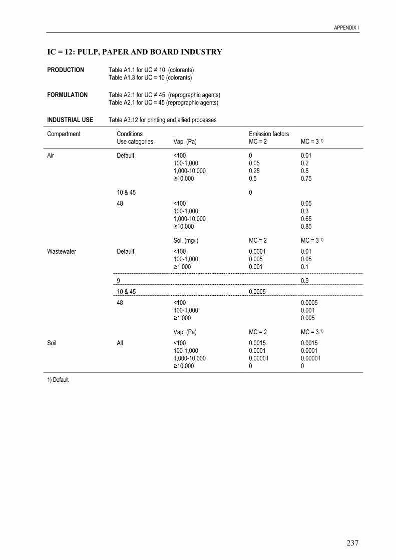
APPENDIX I
237
IC = 12: PULP, PAPER AND BOARD INDUSTRY
PRODUCTION Table A1.1 for UC ≠ 10 (colorants)Table A1.3 for UC = 10 (colorants)
FORMULATION Table A2.1 for UC ≠ 45 (reprographic agents)Table A2.1 for UC = 45 (reprographic agents)
INDUSTRIAL USE Table A3.12 for printing and allied processes
Compartment Conditions Emission factorsUse categories Vap. (Pa) MC = 2 MC = 3 1)
Air Default <100 0 0.01100-1,000 0.05 0.21,000-10,000 0.25 0.5≥10,000 0.5 0.75
10 & 45 048 <100 0.05
100-1,000 0.31,000-10,000 0.65≥10,000 0.85
Sol. (mg/l) MC = 2 MC = 3 1)
Wastewater Default <100 0.0001 0.01100-1,000 0.005 0.05≥1,000 0.001 0.1
9 0.910 & 45 0.000548 <100 0.0005
100-1,000 0.001≥1,000 0.005
Vap. (Pa) MC = 2 MC = 3 1)
Soil All <100 0.0015 0.0015100-1,000 0.0001 0.00011,000-10,000 0.00001 0.00001≥10,000 0 0
1) Default
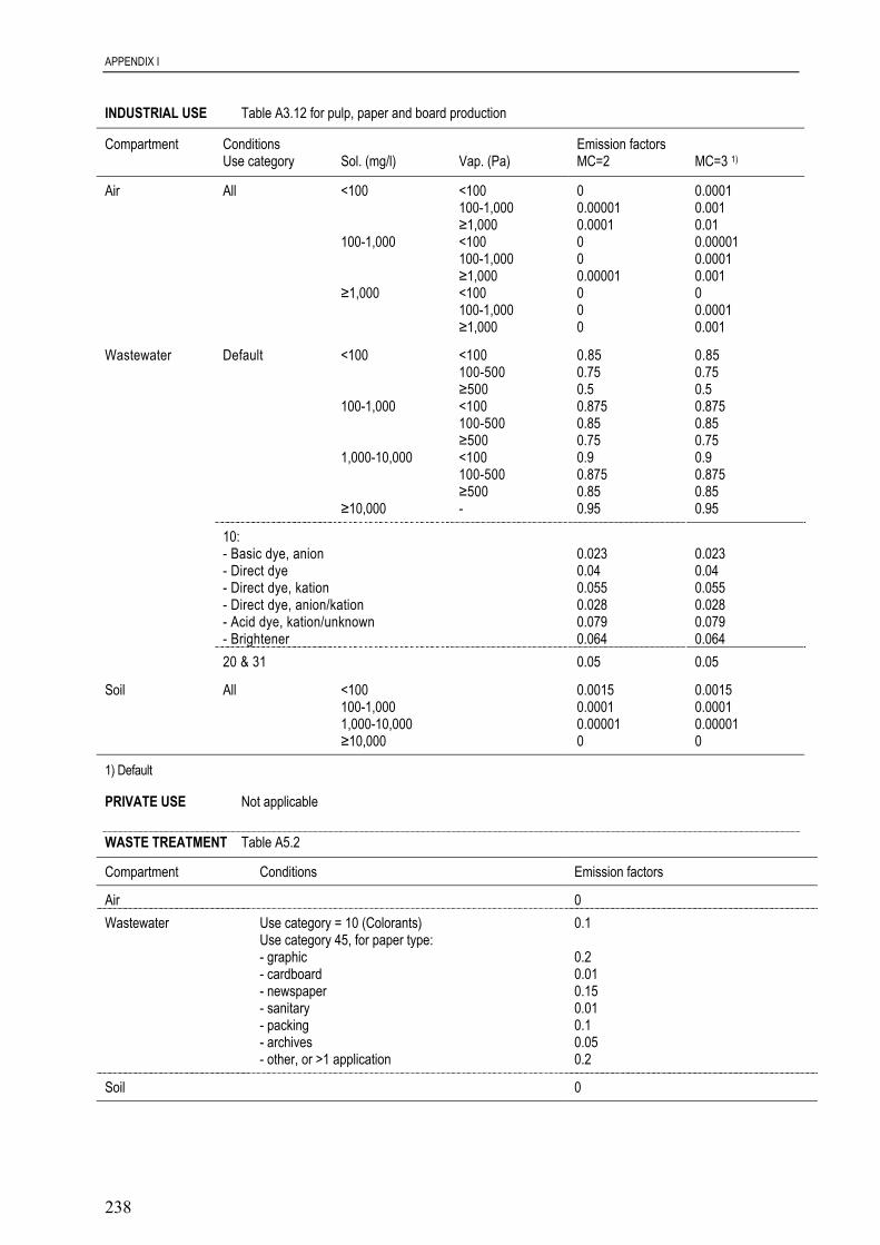
APPENDIX I
238
INDUSTRIAL USE Table A3.12 for pulp, paper and board production
Compartment Conditions Emission factorsUse category Sol. (mg/l) Vap. (Pa) MC=2 MC=3 1)
Air All <100 <100 0 0.0001100-1,000 0.00001 0.001≥1,000 0.0001 0.01
100-1,000 <100 0 0.00001100-1,000 0 0.0001≥1,000 0.00001 0.001
≥1,000 <100 0 0100-1,000 0 0.0001≥1,000 0 0.001
Wastewater Default <100 <100 0.85 0.85100-500 0.75 0.75≥500 0.5 0.5
100-1,000 <100 0.875 0.875100-500 0.85 0.85≥500 0.75 0.75
1,000-10,000 <100 0.9 0.9100-500 0.875 0.875≥500 0.85 0.85
≥10,000 - 0.95 0.95
10:- Basic dye, anion 0.023 0.023- Direct dye 0.04 0.04- Direct dye, kation 0.055 0.055- Direct dye, anion/kation 0.028 0.028- Acid dye, kation/unknown 0.079 0.079- Brightener 0.064 0.06420 & 31 0.05 0.05
Soil All <100 0.0015 0.0015100-1,000 0.0001 0.00011,000-10,000 0.00001 0.00001≥10,000 0 0
1) Default
PRIVATE USE Not applicable
WASTE TREATMENT Table A5.2
Compartment Conditions Emission factors
Air 0Wastewater Use category = 10 (Colorants) 0.1
Use category 45, for paper type:- graphic 0.2- cardboard 0.01- newspaper 0.15- sanitary 0.01- packing 0.1- archives 0.05- other, or >1 application 0.2
Soil 0

APPENDIX I
239
IC = 13: TEXTILE PROCESSING INDUSTRY
PRODUCTION Table A1.1 for UC ≠ 10 (colorants)Table A1.3 for UC = 10 (colorants)
FORMULATION Table A2.1
INDUSTRIAL USE Table A3.14
Compartment Conditions Emission factorsSol. (mg/l) Vap. (Pa) UC<>10 UC = 10
Air <100 <100 0.05100-1,000 0.15≥1,000 0.4
100-1,000 <100 0.025100-1,000 0.05≥1,000 0.15
1,000-10,000 <100 0.01100-1,000 0.025≥1,000 0.05
≥10,000 <100 0.005100-1,000 0.01≥1,000 0.025
Batch dyeing 0.0007Continuous dyeing- thermosol/unknown 0.05- other 0.0025- printing 0.0025
Wastewater <100 <100 0.85100-1,000 0.75≥1,000 0.5
100-1,000 <100 0.875100-1,000 0.85≥1,000 0.75
1,000-10,000 <100 0.9100-1,000 0.875≥1,000 0.85
≥10,000 - 0.95
Table A3.14 continued overleaf
WASTEWATER for UC = 10 (colorants):Emission factor (EF) = Emission factor dyeing process (E.1) + Emission factor “handling, washing out and cleaning” (E.2)
E.1 = A / (1 + K . B) B = 1 / liquor ratio (liquor ratio: default = 10 kg fibres / 1 l solution)A = constantK = equilibrium constant

APPENDIX I
240
INDUSTRIAL USE Table A3.14 Continued
Conditions (UC = 10)Type of dye Type of dyeing K A B E.2
Disperse Continuous 115 5 1 0.055 " Printing 115 2 0.5 0.12Direct Batch 73 1 0.1 1) 0.01Reactive - wool Batch 190 1 0.1 1) 0.01Reactive - cotton Batch 23 1 0.1 1) 0.01Reactive - general Batch 57 1 0.1 1) 0.01Vat Continuous 190 5 1 0.055
Printing 190 2 0.5 0.12Sulphur Continuous 40 5 1 0.055
Printing 40 2 0.5 0.12Acid - one SO3 Batch 90 1 0.1 1) 0.01Acid - > 1 SO3 Batch 190 1 0.1 1) 0.01Basic Batch 990 1 0.1 1) 0.01Azoic (naphtole) Continuous 30 5 1 0.055
Printing 30 2 0.5 0.12Metal complex Batch 150 1 0.1 1) 0.01Pigment Continuous 5000 5 1 0.055
Printing 5000 2 0.5 0.12Unknown, low solubility Continuous 190 5 1 0.055
Printing 190 2 0.5 0.12Unknown, acid groups Batch 90 1 0.1 1) 0.01
1) Default
Compartment Conditions Emission factorsSol. (mg/l) Vap. (Pa) UC<>10 UC = 10
Soil 0.005<100 <100 0.05
100-500 0.15≥500 0.4
≥100 <100 0.025100-500 0.05≥500 0.15
PRIVATE USE Table A4.4
Compartment Conditions Emission factorsSol. (mg/l) UC<>10 UC=10 1)
Air 0Wastewater <250 0.1
250-1,000 0.151,000-5,000 0.2≥5,000 0.3
Soil 0
1) For UC = 10 (Colorants) only, i.e. types used normally by industry for batch dyeing
WASTE TREATMENT Not applicable

APPENDIX I
241
IC = 14: PAINTS, LACQUERS AND VARNISHES INDUSTRY
PRODUCTION Table A1.1
FORMULATION Table A2.1
INDUSTRIAL USE Table A3.15
Compartment Conditions Emission factorsUse category Vap. (Pa) Water based Solvent based
Air 3 110, 14, 20 0 050 047, 52, 55 <10 0 0
10-500 0 0.001500-5,000 0.01 0.05≥5,000 0.05 0.15
48 0.8 0.9
Sol. (mg/l)
Wastewater 3 010, 14, 20 0.005 0.00150 <10 0.005
10-100 0.01≥100 0.05
47, 52, 55 <10 0.005 0.00110-100 0.01 0.005≥100 0.05 0.01
48 0.1 0.02
Soil 3 010, 14, 20 0.005 0.00550 0.00547, 52, 55 0.005 0.00548 0.001 0.001

APPENDIX I
242
PRIVATE USE Table A4.5
Compartment Conditions Emission factorsUse category Vap. (Pa) Water based Solvent based
Air 3 110, 14, 20 0 050 047, 52, 55 <10 0 0
10-500 0 0.001500-5,000 0.01 0.05≥5,000 0.05 0.15
48 0.8 0.95
Sol. (mg/l)
Wastewater 3 010, 14, 20 0.005 0.00150 <10 0.005
10-100 0.01≥100 0.05
47, 52, 55 <10 0.005 0.00110-100 0.01 0.005≥100 0.05 0.01
48 0.15 0.04
Soil 3 010, 14, 20 0.005 0.00550 0.00547, 52, 55 0.005 0.00548 0.01 0.01
WASTE TREATMENT Not applicable

APPENDIX I
243
IC = 16: ENGINEERING INDUSTRY: CIVIL AND MECHANICAL
PRODUCTION Table A1.1
FORMULATION Table A2.1
INDUSTRIAL USE Table A3.16
Compartment Conditions Emission factorsSol. (mg/l) Vap. (Pa) MC=2 MC=3 1) MC =4
Air <100 <10 0.0001 0.001 0.0110-100 0.001 0.01 0.1100-1,000 0.01 0.1 0.251,000-10,000 0.1 0.5 0.7≥10,000 0.5 0.75 0.9
100-1000 <10 0.00001 0.0001 0.00110-100 0.0001 0.001 0.05100-1,000 0.001 0.05 0.11,000-10,000 0.05 0.1 0.5≥10,000 0.25 0.5 0.75
≥1,000 <10 0 0.00001 0.000110-100 0.00001 0.0001 0.001100-1,000 0.0001 0.001 0.011,000-10,000 0.001 0.01 0.1≥10,000 0.01 0.1 0.5
Wastewater <100 <10 0.01 0.1 0.510-100 0.001 0.01 0.1100-1,000 0.0001 0.001 0.011,000-10,000 0.00001 0.0001 0.001≥10,000 0 0.00001 0.0001
100-1000 <10 0.25 0.5 0.7510-100 0.05 0.1 0.5100-1,000 0.001 0.01 0.11,000-10,000 0.0001 0.001 0.05≥10,000 0.00001 0.0001 0.001
≥1,000 <10 0.5 0.75 0.910-100 0.1 0.5 0.7100-1,000 0.01 0.1 0.251,000-10,000 0.001 0.01 0.1≥10,000 0.0001 0.001 0.01
Soil <100 <10 0.005 0.01 0.0510-100 0.001 0.005 0.01100-1,000 0.0005 0.001 0.0051,000-10,000 0 0.0005 0.001≥10,000 0 0 0.0005
100-1000 <10 0.001 0.005 0.0110-100 0.0005 0.001 0.005100-1,000 0 0.0005 0.0011,000-10,000 0 0 0.0005≥10,000 0 0 0.0001
≥1,000 <10 0.0005 0.001 0.00510-100 0 0.0005 0.001100-1,000 0 0 0.00051,000-10,000 0 0 0.0001≥10,000 0 0 0
1) Default

APPENDIX I
244
PRIVATE USE Table A3.16
WASTE TREATMENT Not applicable

APPENDIX I
245
IC = 0: OTHERS
PRODUCTION Table A1.1
FORMULATION Table A2.1
INDUSTRIAL USE Table A3.16

APPENDIX I
246
B-tables
Estimates for the fraction of the main source and the number of days for emissions

APPENDIX I
247
IC = 1: AGRICULTURAL INDUSTRY
PRODUCTION Table B1.1 for new substances and existing substances other than HPVC for UC ≠ 38 & 41
T (tonnes/year) f main source No. of days
<1,000 1 0.1f.T1,000-2,000 0.9 0.1f.T2,000-4.000 0.75 0.1f.T≥4,000 0.7 300
PRODUCTION Table B1.2 for new substances and existing substances other than HPVC For UC = 38 & 41
T (tonnes/year) f main source No. of days
<10 1 f.T10-50 0.9 f.T50-100 0.8 0.6667f.T100-1,000 0.75 0.4f.T1,000-2,500 0.6 0.2f.T≥2,500 0.6 300
PRODUCTION Table B1.3 for HPVC (default ≥10,000)for UC ≠ 38 & 41
T (tonnes/year) f main source No. of days
<25,000 1 30025,000-100,000 0.75 300>100,000 0.6 300
PRODUCTION Table B1.4 for HPVC (default ≥3,500)for UC = 38 & 41
T (tonnes/year) f main source No. of days
<5,000 1 3005,000-25,000 0.8 30025,000-100,000 0.6 300≥100,000 0.4 300
FORMULATION Table B2.1 for new substances and existing substances other than HPVC
T (tonnes/year) F main source No. of days
<100 1 2f.T100-500 0.6 f.T500-1,000 0.6 0.5f.T≥1,000 0.4 300

APPENDIX I
248
FORMULATION Table B2.2 for HPVC for UC ≠ 38 & 41
T (tonnes/year) f main source No. of days
<15,000 1 30015,000-50,000 0.75 300≥50,000 0.6 300
FORMULATION Table B2.3 for HPVC for UC = 38 & 41
T (tonnes/year) f main source No. of days
<3,500 1 3003,500-10,000 0.8 30010,000-25,000 0.7 30025,000-50,000 0.6 300≥50,000 0.4 300
INDUSTRIAL USE Table B3.1
T (tonnes/year) f main source No. of days for use categories:3,19,39,48,50 41 9,10,36 26
<10 0.05 2 10 50 30010-100 0.01 2 10 50 300100-1,000 0.005 2 10 50 3001,000-10,000 0.001 2 10 50 30010,000-50,000 0.0005 2 10 50 300≥50,000 0.00001 2 10 50 300
PRIVATE USE Not applicable
WASTE TREATMENT Not applicable

APPENDIX I
249
IC = 2: CHEMICAL INDUSTRY: BASIC CHEMICALS
PRODUCTION Table B1.1 for non-HPVCTable B1.5 for HPVC (default ≥10,000)
T (tonnes/year) f main source No. of days
<25,000 1 30025,000-100,000 0.75 300100,000-500,000 0.6 300≥500,000 0.5 300
FORMULATION Table B2.4 for non-HPVCIf applicable! T (tonnes/year) f main source No. of days
<10 1 2f.T10-50 0.9 f.T50-500 0.8 0.4f.T500-2,000 0.75 0.2f.T≥2,000 0.65 300
FORMULATION Table B2.5 for HPVCIf applicable!T (tonnes/year) f main source No. of days
<25,000 1 30025,000-50,000 0.75 300≥50,000 0.4 300
INDUSTRIAL USE Table B3.2
T (tonnes/year) F MAIN SOURCE NO. OF DAYS
<10 0.8 2f.T10-50 0.65 f.T50-500 0.5 0.4f.T500-2,000 0.4 0.25f.T2,000-5,000 0.3 0.2f.T5,000-25,000 0.25 30025,000-75,000 0.2 300≥75,000 0.15 300
PRIVATE USE Not applicable
WASTE TREATMENT Not applicable

APPENDIX I
250
IC = 3: CHEMICAL INDUSTRY: CHEMICALS USED IN SYNTHESIS
PRODUCTION Table B1.2 for non-HPVCTable B1.6 for HPVC (default ≥7,000)
T (tonnes/year) f main source No. of days
<10,000 1 30010,000-50,000 0.75 30050,000-250,000 0.6 300≥250,000 0.5 300
FORMULATION Table B2.4 for non-HPVCTable B2.3 for HPVC
If applicable!
INDUSTRIAL USE Table B3.2
PRIVATE USE Not applicable
WASTE TREATMENT Not applicable

APPENDIX I
251
IC = 4: ELECTRICAL/ELECTRONIC INDUSTRY
PRODUCTION Table B1.7 for non-HPVC
T (tonnes/year) f main source No. of days
<100 1 0.1f.T100-1,000 0.9 0.1f.T1,000-2,500 0.8 0.1f.T≥2,500 0.75 300
PRODUCTION Table B1.6 for HPVC (default ≥7,000)
FORMULATION Table B2.4 for non-HPVCTable B2.3 for HPVC
INDUSTRIAL USE Table B3.2
PRIVATE USE Not applicable
WASTE TREATMENT Not applicable
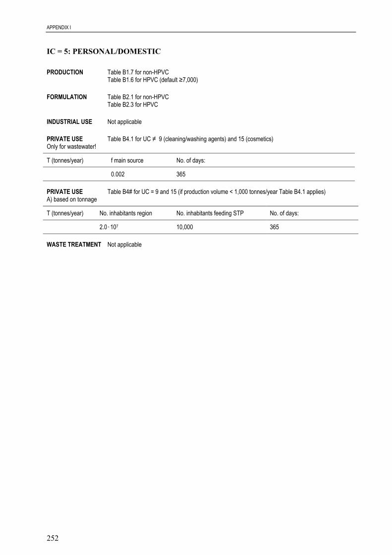
APPENDIX I
252
IC = 5: PERSONAL/DOMESTIC
PRODUCTION Table B1.7 for non-HPVCTable B1.6 for HPVC (default ≥7,000)
FORMULATION Table B2.1 for non-HPVCTable B2.3 for HPVC
INDUSTRIAL USE Not applicable
PRIVATE USE Table B4.1 for UC ≠ 9 (cleaning/washing agents) and 15 (cosmetics)Only for wastewater!
T (tonnes/year) f main source No. of days:
0.002 365
PRIVATE USE Table B4# for UC = 9 and 15 (if production volume < 1,000 tonnes/year Table B4.1 applies)A) based on tonnage
T (tonnes/year) No. inhabitants region No. inhabitants feeding STP No. of days:
2.0.107 10,000 365
WASTE TREATMENT Not applicable
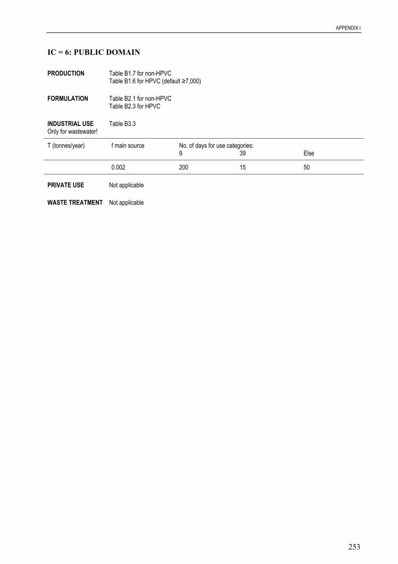
APPENDIX I
253
IC = 6: PUBLIC DOMAIN
PRODUCTION Table B1.7 for non-HPVCTable B1.6 for HPVC (default ≥7,000)
FORMULATION Table B2.1 for non-HPVCTable B2.3 for HPVC
INDUSTRIAL USE Table B3.3Only for wastewater!
T (tonnes/year) f main source No. of days for use categories:9 39 Else
0.002 200 15 50
PRIVATE USE Not applicable
WASTE TREATMENT Not applicable

APPENDIX I
254
IC = 7: LEATHER PROCESSING INDUSTRY
PRODUCTION Table B1.8 for non-HPVC for UC ≠ 6, 9 10 & 31
T (tonnes/year) f main source No. of days
<1,000 1 0.1f.T1,000-4,000 0.9 0.1f.T≥4,000 0.75 300
PRODUCTION Table B1.9 for non-HPVC for UC = 6, 9 10 & 31
T (tonnes/year) f main source No. of days
<10 1 f.T10-50 0.9 f.T50-500 0.5 f.T500-1,500 0.2 f.T≥1,500 0.2 300
PRODUCTION Table B1.4 for HPVC (default ≥5,000) for UC ≠ 6, 9 10 & 31Table B1.4 for HPVC (default ≥2,500) for UC = 6, 9 10 & 31
FORMULATION Table B2.4 for non-HPVCTable B2.3 for HPVC for UC ≠ 6, 9, 10 & 31Table B2.6 for HPVC for UC = 6, 9, 10 & 31
T (tonnes/year) f main source No. of days
<100,000 1 300100,000-250,000 0.7 300≥250,000 0.4 300
INDUSTRIAL USE Table B3.4
T (tonnes/year) f main source No. of days
<10 0.8 2f.T10-50 0.75 2f.T50-500 0.6 f.T500-1,500 0.5 0.4f.T1,500-5,000 0.35 3005,000-25,000 0.2 300≥25,000 0.1 300
PRIVATE USE Not applicable
WASTE TREATMENT Not applicable

APPENDIX I
255
IC = 8: METAL EXTRACTION, REFINING AND PROCESSING INDUSTRY
PRODUCTION Table B1.2 for non-HPVC for UC ≠ 29 & 35Table B1.10 for non-HPVC for UC = 29 & 35
T (tonnes/year) f main source No. of days
<10 1 f.T10-50 0.9 f.T50-500 0.8 0.6667f.T500-1,500 0.5 0.4f.T≥1,500 0.5 300
PRODUCTION Table B1.6 for HPVC (default ≥7,000) for UC ≠ 29 & 35Table B1.4 for HPVC (default ≥2,500) for UC = 29 & 35
FORMULATION Table B2.4 for non-HPVCTable B2.3 for HPVC
INDUSTRIAL USE Table B3.5 for UC = 29 & 35
T (tonnes/year) No. of days f main Field of applicationsource: Primary steelworks Else
<1,000 300 1 0.81,000-5,000 300 0.9 0.55,000-50,000 300 0.75 0.3≥50,000 300 0.6 0.2
INDUSTRIAL USE Table B3.6 for UC ≠ 29 & 35
T (tonnes/year) f main source No. of days
<10 1 2f.T10-50 1 0.5f.T50-500 0.9 0.4f.T500-2,000 0.8 0.1875f.T2,000-10,000 0.7 30010,000-50,000 0.6 300≥50,000 0.5 300
PRIVATE USE Not applicable
WASTE TREATMENT Not applicable

APPENDIX I
256
IC = 9: MINERAL OIL AND FUEL INDUSTRY
PRODUCTION Table B1.1 for non-HPVC for UC = 27Table B1.2 for non-HPVC for UC = 28+othersTable B1.4 for HPVC (default ≥3,000) for UC = 28+othersTable B1.11 for HPVC (default ≥25,000) for UC = 27
T (tonnes/year) f main source No. of days
<100,000 1 300100,000-500,000 0.75 300≥500,000 0.5 300
FORMULATION Table B2.7 for non-HPVC for UC = 27
T (tonnes/year) f main source No. of days
<1,000 1 1001,000-2,000 0.8 200≥2,000 0.6 300
FORMULATION Table B2.8 for non-HPVC for UC = 28+others
T (tonnes/year) f main source No. of days
<5 1 205-50 1 6050-100 1 2f.T100-500 0.8 f.T500-1,000 0.6 0.5f.T≥1,000 0.4 300
FORMULATION Table B2.6 for HPVC for UC = 27Table B2.6 for HPVC for UC = 28+others
INDUSTRIAL USE Table B3.7
T (tonnes/year) f main source No. of days
<50 0.5 35050-500 0.4 350500-5,000 0.3 3505,000-25,000 0.2 35025000-100,000 0.05 350≥100,000 0.02 350
PRIVATE USE Table 4.1Only for wastewater!
WASTE TREATMENT Not applicable

APPENDIX I
257
IC = 10: PHOTOGRAPHIC INDUSTRY
PRODUCTION Table B1.4 for HPVC (default ≥4,000)Table B1.12 for non-HPVC
T (tonnes/year) f main source No. of days
<5 1 f.T5-50 1 0.5f.T50-250 0.75 0.4f.T250-3,000 0.5 0.2f.T≥3,000 0.5 300
FORMULATION Table B2.8 for non-HPVCTable B2.3 for HPVC
INDUSTRIAL USE Table B3.8
Company size f main source No. of days
One company 1 300 (No private use)Large companies 0.333 300 (No private use)Small companies 0.05 300
PRIVATE USE Table B4.2Only for wastewater!Only if company size at industrial use is small companies (otherwise f main source is zero)F main source = 0.002.f private use
T (tonnes/year) f private use F main source No. of days:
<10 0 0 20010-50 0.00002 4.10-8 20050-500 0.0001 2.10-7 200500-5,000 0.0005 1.10-6 200≥5,000 0.0025 5.10-6 200
WASTE TREATMENT Table B5.1
T (tonnes/year) f main source No. of days One company
<10 1 150 (No private use)≥10 1 300
T (tonnes/year) f main source No. of days Large companies
<30 0.333 150≥30 0.333 300
T (tonnes/year) f main source No. of days Small companies
<200 0.2 150≥200 0.2 300
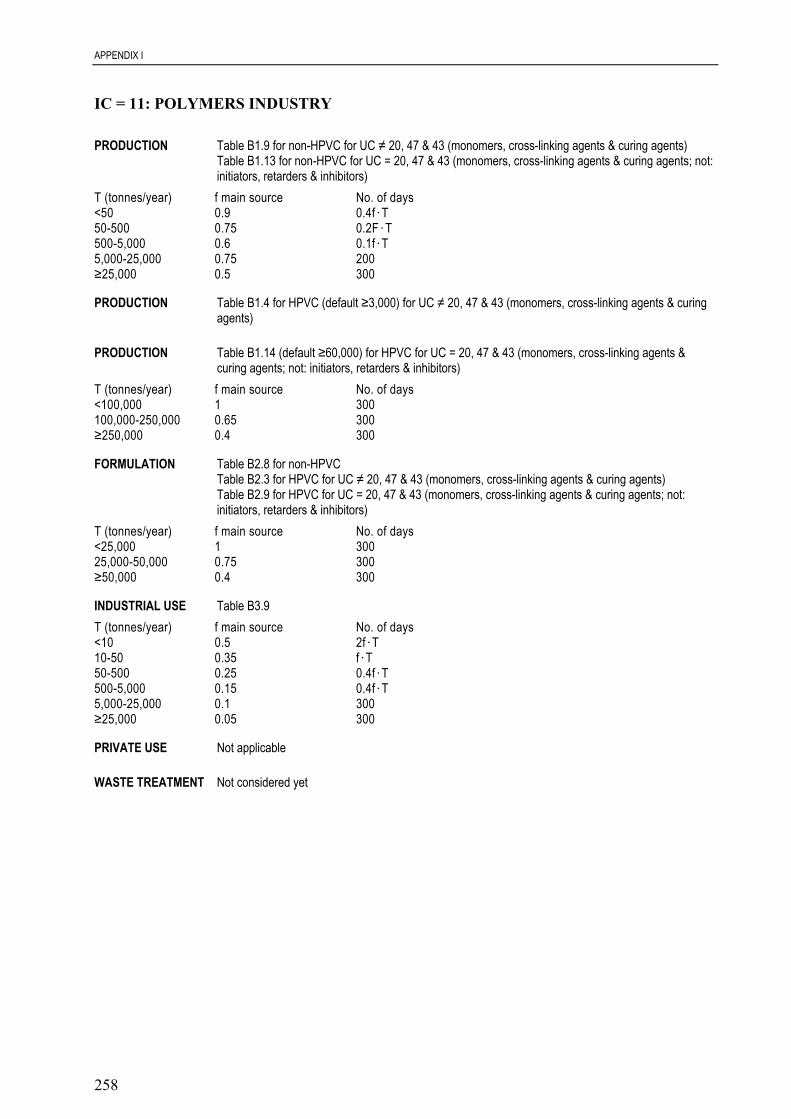
APPENDIX I
258
IC = 11: POLYMERS INDUSTRY
PRODUCTION Table B1.9 for non-HPVC for UC ≠ 20, 47 & 43 (monomers, cross-linking agents & curing agents)Table B1.13 for non-HPVC for UC = 20, 47 & 43 (monomers, cross-linking agents & curing agents; not:initiators, retarders & inhibitors)
T (tonnes/year) f main source No. of days<50 0.9 0.4f.T50-500 0.75 0.2F.T500-5,000 0.6 0.1f.T5,000-25,000 0.75 200≥25,000 0.5 300
PRODUCTION Table B1.4 for HPVC (default ≥3,000) for UC ≠ 20, 47 & 43 (monomers, cross-linking agents & curingagents)
PRODUCTION Table B1.14 (default ≥60,000) for HPVC for UC = 20, 47 & 43 (monomers, cross-linking agents &curing agents; not: initiators, retarders & inhibitors)
T (tonnes/year) f main source No. of days<100,000 1 300100,000-250,000 0.65 300≥250,000 0.4 300
FORMULATION Table B2.8 for non-HPVCTable B2.3 for HPVC for UC ≠ 20, 47 & 43 (monomers, cross-linking agents & curing agents)Table B2.9 for HPVC for UC = 20, 47 & 43 (monomers, cross-linking agents & curing agents; not:initiators, retarders & inhibitors)
T (tonnes/year) f main source No. of days<25,000 1 30025,000-50,000 0.75 300≥50,000 0.4 300
INDUSTRIAL USE Table B3.9T (tonnes/year) f main source No. of days<10 0.5 2f.T10-50 0.35 f.T50-500 0.25 0.4f.T500-5,000 0.15 0.4f.T5,000-25,000 0.1 300≥25,000 0.05 300
PRIVATE USE Not applicable
WASTE TREATMENT Not considered yet
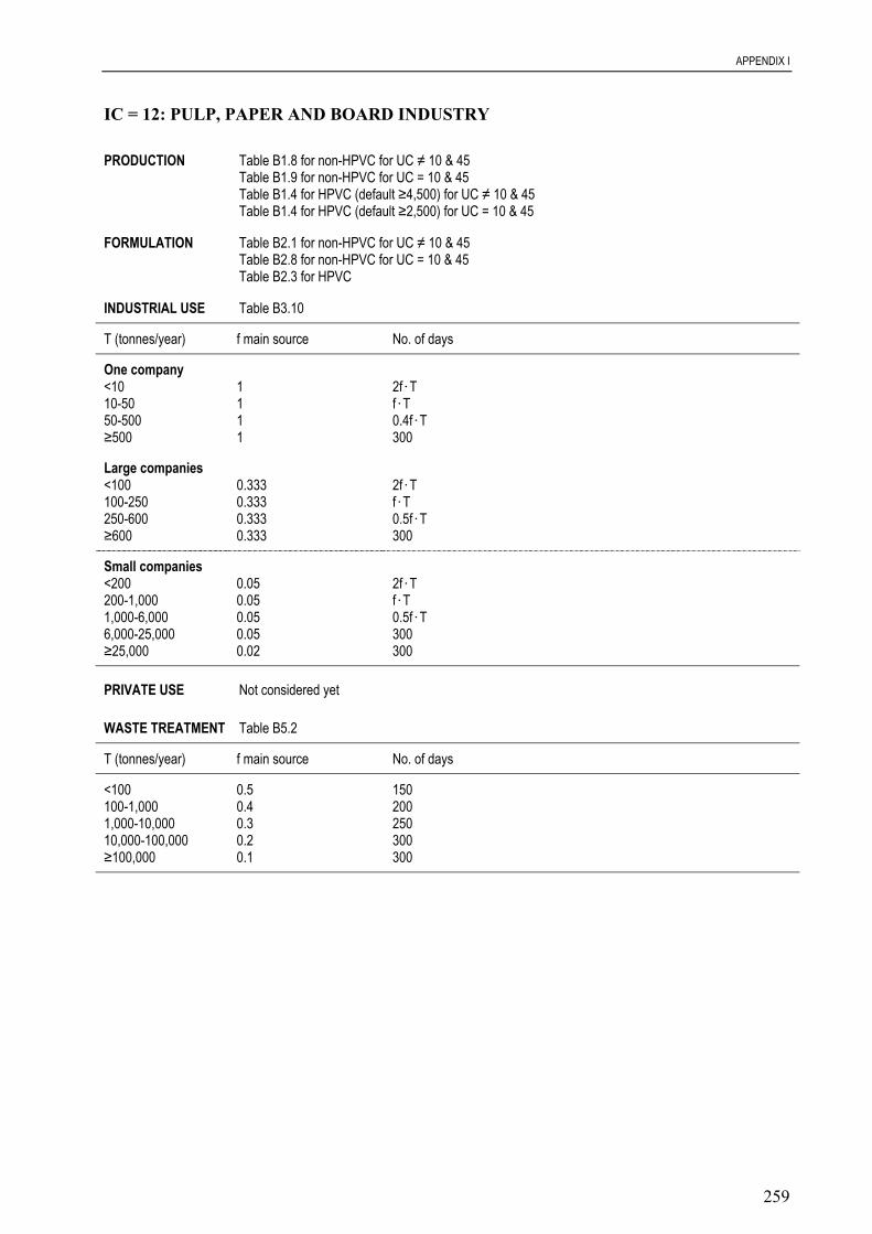
APPENDIX I
259
IC = 12: PULP, PAPER AND BOARD INDUSTRY
PRODUCTION Table B1.8 for non-HPVC for UC ≠ 10 & 45Table B1.9 for non-HPVC for UC = 10 & 45Table B1.4 for HPVC (default ≥4,500) for UC ≠ 10 & 45Table B1.4 for HPVC (default ≥2,500) for UC = 10 & 45
FORMULATION Table B2.1 for non-HPVC for UC ≠ 10 & 45Table B2.8 for non-HPVC for UC = 10 & 45Table B2.3 for HPVC
INDUSTRIAL USE Table B3.10
T (tonnes/year) f main source No. of days
One company<10 1 2f.T10-50 1 f.T50-500 1 0.4f.T≥500 1 300
Large companies<100 0.333 2f.T100-250 0.333 f.T250-600 0.333 0.5f.T≥600 0.333 300
Small companies<200 0.05 2f.T200-1,000 0.05 f.T1,000-6,000 0.05 0.5f.T6,000-25,000 0.05 300≥25,000 0.02 300
PRIVATE USE Not considered yet
WASTE TREATMENT Table B5.2
T (tonnes/year) f main source No. of days
<100 0.5 150100-1,000 0.4 2001,000-10,000 0.3 25010,000-100,000 0.2 300≥100,000 0.1 300
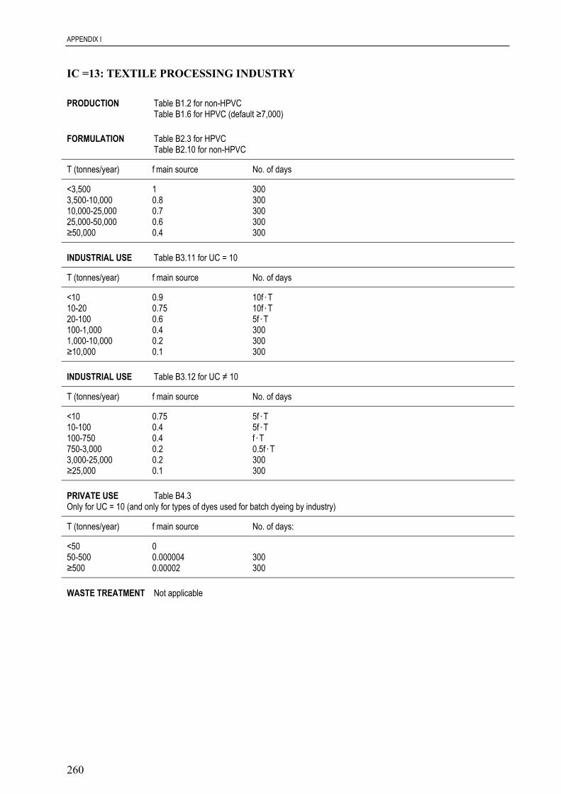
APPENDIX I
260
IC =13: TEXTILE PROCESSING INDUSTRY
PRODUCTION Table B1.2 for non-HPVCTable B1.6 for HPVC (default ≥7,000)
FORMULATION Table B2.3 for HPVCTable B2.10 for non-HPVC
T (tonnes/year) f main source No. of days
<3,500 1 3003,500-10,000 0.8 30010,000-25,000 0.7 30025,000-50,000 0.6 300≥50,000 0.4 300
INDUSTRIAL USE Table B3.11 for UC = 10
T (tonnes/year) f main source No. of days
<10 0.9 10f.T10-20 0.75 10f.T20-100 0.6 5f.T100-1,000 0.4 3001,000-10,000 0.2 300≥10,000 0.1 300
INDUSTRIAL USE Table B3.12 for UC ≠ 10
T (tonnes/year) f main source No. of days
<10 0.75 5f.T10-100 0.4 5f.T100-750 0.4 f.T750-3,000 0.2 0.5f.T3,000-25,000 0.2 300≥25,000 0.1 300
PRIVATE USE Table B4.3Only for UC = 10 (and only for types of dyes used for batch dyeing by industry)
T (tonnes/year) f main source No. of days:
<50 050-500 0.000004 300≥500 0.00002 300
WASTE TREATMENT Not applicable
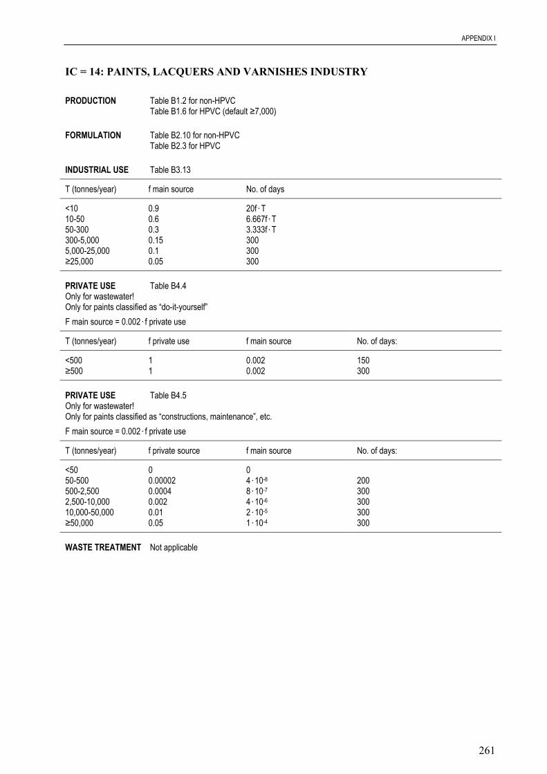
APPENDIX I
261
IC = 14: PAINTS, LACQUERS AND VARNISHES INDUSTRY
PRODUCTION Table B1.2 for non-HPVCTable B1.6 for HPVC (default ≥7,000)
FORMULATION Table B2.10 for non-HPVCTable B2.3 for HPVC
INDUSTRIAL USE Table B3.13
T (tonnes/year) f main source No. of days
<10 0.9 20f.T10-50 0.6 6.667f.T50-300 0.3 3.333f.T300-5,000 0.15 3005,000-25,000 0.1 300≥25,000 0.05 300
PRIVATE USE Table B4.4Only for wastewater!Only for paints classified as “do-it-yourself”F main source = 0.002.f private use
T (tonnes/year) f private use f main source No. of days:
<500 1 0.002 150≥500 1 0.002 300
PRIVATE USE Table B4.5Only for wastewater!Only for paints classified as “constructions, maintenance”, etc.F main source = 0.002.f private use
T (tonnes/year) f private source f main source No. of days:
<50 0 050-500 0.00002 4.10-8 200500-2,500 0.0004 8.10-7 3002,500-10,000 0.002 4.10-6 30010,000-50,000 0.01 2.10-5 300≥50,000 0.05 1.10-4 300
WASTE TREATMENT Not applicable
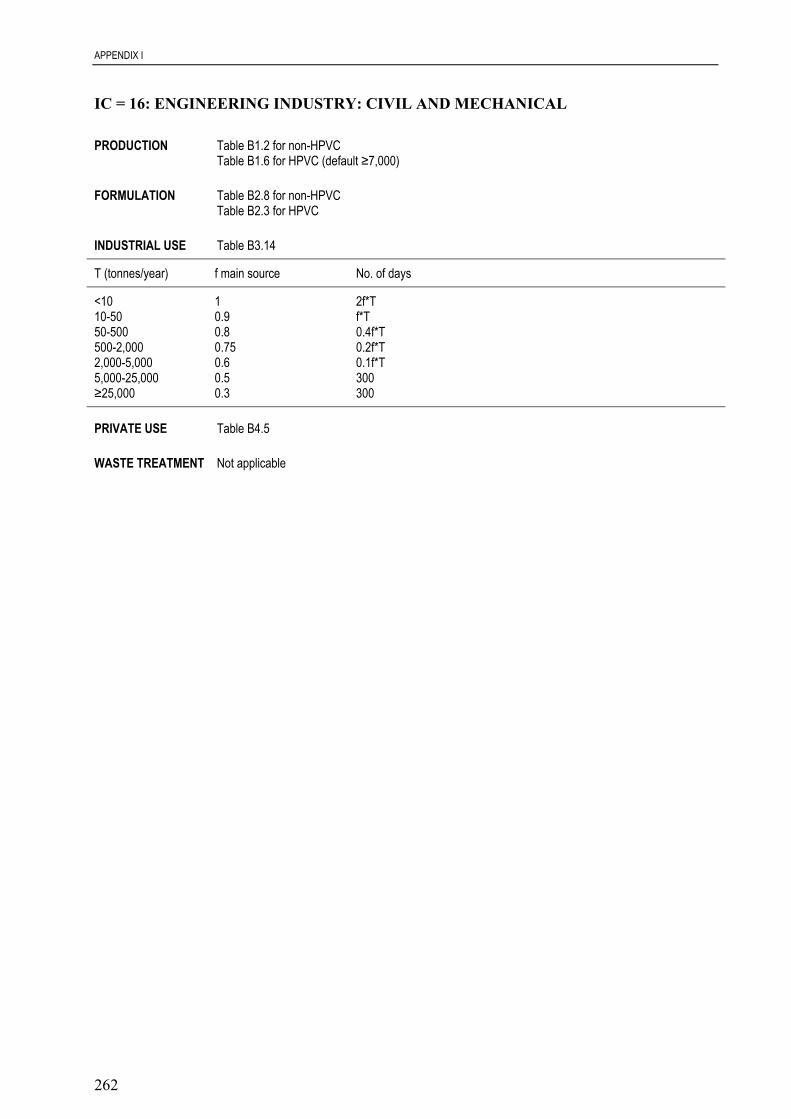
APPENDIX I
262
IC = 16: ENGINEERING INDUSTRY: CIVIL AND MECHANICAL
PRODUCTION Table B1.2 for non-HPVCTable B1.6 for HPVC (default ≥7,000)
FORMULATION Table B2.8 for non-HPVCTable B2.3 for HPVC
INDUSTRIAL USE Table B3.14
T (tonnes/year) f main source No. of days
<10 1 2f*T10-50 0.9 f*T50-500 0.8 0.4f*T500-2,000 0.75 0.2f*T2,000-5,000 0.6 0.1f*T5,000-25,000 0.5 300≥25,000 0.3 300
PRIVATE USE Table B4.5
WASTE TREATMENT Not applicable
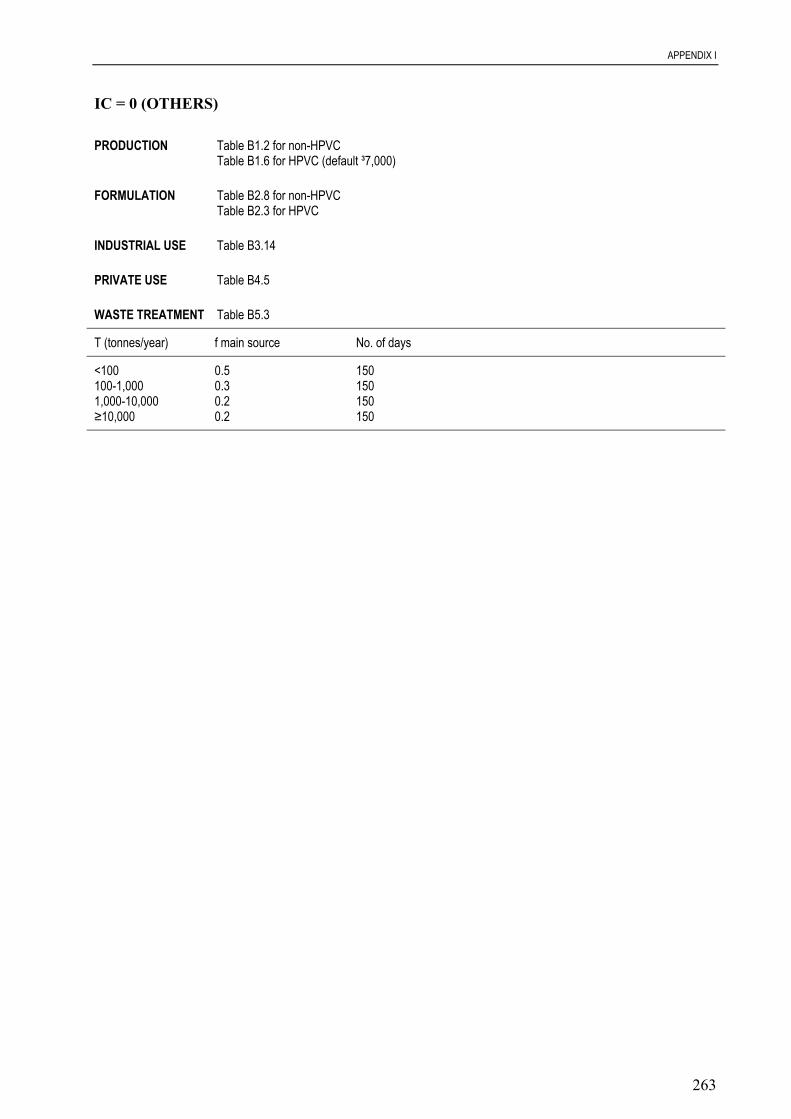
APPENDIX I
263
IC = 0 (OTHERS)
PRODUCTION Table B1.2 for non-HPVCTable B1.6 for HPVC (default ³7,000)
FORMULATION Table B2.8 for non-HPVCTable B2.3 for HPVC
INDUSTRIAL USE Table B3.14
PRIVATE USE Table B4.5
WASTE TREATMENT Table B5.3
T (tonnes/year) f main source No. of days
<100 0.5 150100-1,000 0.3 1501,000-10,000 0.2 150≥10,000 0.2 150

APPENDIX I
264
Appendix I-a: List of synonyms for functions according to ChemUSES (US EPA, 1980)
No. Use Category No. Function (ChemUSES)
1 Absorbents and adsorbents 131 Absorbents60 Adsorbents213 Dehumidifiers
2 Adhesive, binding agents 302 Adhesives143 Binders145 Food additives92 Spreaders165 Stickers280 Tackifiers
3 Aerosol propellants 178 Aerosol propellants4 Anti-condensation agents
5 Anti-freezing agents 77 Antifreezes74 De-icers52 Deodorants313 Functional fluids
6 Anti-set-off and anti-adhesive agents 104 Abherents63 Antiblocking agents188 Anticaking agents300 Detackifiers233 Dusting agents144 Parting agents7 Soil retardants
7 Anti-static agents 328 Antistatic agents89 Electroconductive coating agents318 Humectants
8 Bleaching agents 304 Bleaching assistants132 Bleaching agents
9 Cleaning/washing agents and additives 293 Antiredeposition agents180 Boil-off assistants242 Cleaners173 Detergents78 Pre-spotting agents274 Scouring agents261 Shrinkage controllers14 Soaping-off assistants294 Soil release agents
10 Colouring agents 5 Bloom agents86 Colouring agents174 Coupling agents (dyes)267 Dyes20 Fluorescent agents248 Lakes381 Luminescent agents235 Mercerising assistants128 Opacifiers139 Pearlizing agents125 Pigments83 Stains

APPENDIX I
265
No. Use Category No. Function (ChemUSES)
11 Complexing agents 177 Antiprecipitants124 Complexing agents10 Sequestering agents
12 Conductive agents 161 Electrical conductive agents383 Electrode materials245 Electrolytes313 Functional fluids
13 Construction materials and additives 324 Case-hardening agents355 Concrete additives361 Embrittlement inhibitors375 Materials for shaping250 Reinforcing agents349 Water-reducing agents
14 Corrosion inhibitors 230 Antioxidants64 Antiscaling agents323 Corrosion inhibitors
15 Cosmetics 301 Antiperspirants167 Cosmetic ingredients
16 Dust binding agents 26 Dust control agents
17 Electroplating agents 353 Brighteners32 Fume suppressants
18 Explosives 179 Detonators363 Explosion inhibitors158 Explosives27 Incendiaries
19 Fertilisers 34 Fertilisers
20 Fillers 351 Fillers (augmentation)212 Fillers (patching)371 Surface coating additives127 Swelling agents58 Weighting agents (textile technology)
21 Fixing agents 291 Anticrock agents347 Antistripping agents268 Barrier coating agents295 Fixatives134 Fixing agents (fragrances)112 Fixing agents (textile technology)227 Mordents
22 Flame retardants and fire preventing agents 25 Fire extinguishing agents332 Flame retardants
23 Flotation agents 163 Activators (ore processing)190 Flocculating agents297 Flotation agents360 Modifiers
24 Flux agents for casting
25 Foaming agents 358 Blowing agents133 Chemical blowing agents94 Frothers50 Physical blowing agents

APPENDIX I
266
No. Use Category No. Function (ChemUSES)
26 Food/feedstuff additives 214 Acidulants66 Feed additives80 Sweeteners (taste)
27 Fuels 247 Fuels
28 Fuel additives 329 Antifouling agents76 Antiknock agents183 Deposit modifiers306 Fuel additives138 Sweeteners (petroleum technology)
29 Heat transferring agents 72 Coolants313 Functional fluids199 Heat transfer agents216 Quenchers208 Refrigerants
30 Hydraulic fluids and additives 313 Functional fluids65 Hydraulic fluids256 Transmission fluids
31 Impregnation agents 102 Delustrants98 Sizes258 Water repellents23 Waterproofing agents
32 Insulating materials 254 Acoustical insulating material311 Electrical insulating material314 Heat insulating materials162 Insulating materials
33 Intermediates 146 Inorganic intermediates115 Monomers290 Organic intermediates43 Prepolymers
34 Laboratory chemicals 238 Analytical and product testing122 Chelating agents107 Deionisers373 Extraction agents69 Indicators325 Oxidation-reduction indicators374 Reagents
35 Lubricants and additives 119 Antiseize agents313 Functional fluids148 Internal lubricating agents195 Lubricant additives364 Lubricating agents346 Oiliness agents249 Penetrants312 Slip agents
36 Odour agents 79 Flavours and fragrances339 Odorants

APPENDIX I
267
No. Use Category No. Function (ChemUSES)
37 Oxidising agents 149 Oxidisers
38 Plant protection products, agricultural 166 Animal repellents333 Bactericides108 Biocides97 Decontaminats270 Fumigants362 Fungicides275 Herbicides155 Insect attractants348 Insect repellents330 Insecticides252 Nematocides253 Pesticides264 Rodenticides
39 Biocides, non-agricultural 287 Algicides1 Antifouling agents140 Disinfectants118 Preservatives116 Slime preventatives
40 PH-regulating agents 172 Laundry sours266 pH control agents191 pH indicators
41 Pharmaceuticals
42 Photochemicals 122 Chelating agents198 Desensitisers (explosives)299 Desensitisers (photography)182 Developers286 Intensifiers (photography)285 Light stabilisers344 Photosensitive agents303 Sensitisers
43 Process regulators 321 Accelerators46 Activators (chemical processes)239 Activators (enzymes)110 Adhesion promoters4 Antifelting agents352 Antislip finishing agents206 Antistaining agents194 Antiwebbing agents281 Builders222 Carbonising agents164 Carriers19 Catalyst supports170 Catalysts31 Chain extenders113 Chain terminators141 Chain transfer agents122 Chelating agents114 Coagulants278 Coalescents357 Coalescing agents
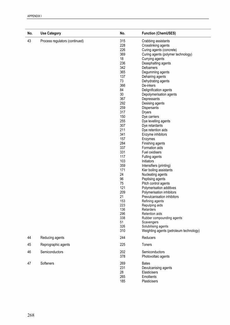
APPENDIX I
268
No. Use Category No. Function (ChemUSES)
43 Process regulators (continued) 315 Crabbing assistants228 Crosslinking agents226 Curing agents (concrete)369 Curing agents (polymer technology)18 Currying agents236 Deasphalting agents342 Defoamers365 Degumming agents137 Dehairing agents73 Dehydrating agents366 De-inkers84 Delignification agents30 Depolymerisation agents367 Depressants292 Desising agents259 Dispersants317 Dryers150 Dye carriers255 Dye levelling agents307 Dye retardants211 Dye retention aids341 Enzyme inhibitors157 Enzymes284 Finishing agents337 Formation aids331 Fuel oxidisers117 Fulling agents103 Initiators359 Intensifiers (printing)171 Kier boiling assistants24 Nucleating agents96 Peptising agents75 Pitch control agents121 Polymerisation additives209 Polymerisation inhibitors21 Prevulcanisation inhibitors153 Refining agents223 Repulping aids136 Retarders296 Retention aids338 Rubber compounding agents51 Scavengers326 Solubilising agents310 Weighting agents (petroleum technology)
44 Reducing agents 244 Reducers
45 Reprographic agents 225 Toners
46 Semiconductors 202 Semiconductors378 Photovoltaic agents
47 Softeners 269 Bates231 Devulcanising agents28 Elasticisers265 Emollients185 Plasticisers

APPENDIX I
269
No. Use Category No. Function (ChemUSES)
47 Softeners (continued) 29 Softeners147 Water softeners
48 Solvents 229 Degreasers82 Dewaxing solvents373 Extraction agents320 Paint and varnish removers16 Reaction media271 Solvents
49 Stabilisers 277 Anticracking agents12 Antifume agents129 Antihydrolysis agents168 Antiozonants230 Antioxidants120 Antilivering agents282 Antiplasticisers160 Antisagging agents68 Antisettling agents88 Bloom inhibitors123 Coupling agents (polymers)159 Emulsifiers87 Heat stabilisers54 Stabilisers36 Ultraviolet absorbers
50 Surface-active agents 41 Antifloating agents234 Antifogging agents109 Surfactants243 Wetting agents
51 Tanning agents 316 Tanning agents
52 Viscosity adjustors 152 Antiflooding agents120 Antilivering agents343 Antiskinning agents221 Gelling agents262 Pour point depressants272 Thickeners334 Thixotropic agents240 Turbulence suppressors135 Viscosity adjustors15 Viscosity index improvers
53 Vulcanising agents 288 Vulcanising agents
54 Welding and soldering agents 101 Brazing agents22 Fluxing agents
0 Other 204 Ablatives105 Abrasives196 Activators (luminescence)354 Aerating agents47 Air entraining agents376 Alloying agents90 Anticratering agents48 Anticreasing agents99 Antifogging agents

APPENDIX I
270
No. Use Category No. Function (ChemUSES)
0 Other (continued) 218 Antipilling agents350 Antiskid agents6 Blasting abrasives70 Bluing agents220 Bright dips93 Chemical raw materials298 Clarifiers260 Cloud point depressants130 Coating agents283 Collectors335 Coupling agents (solutions)215 Culture nutrients81 Deaerating agents309 Deblooming agents85 Dechlorinating agents73 Dehydrating agents107 Deionisers232 Demulsifiers200 Denaturants49 Descaling agents205 Dewatering aids356 Discharge printing agents38 Drainage aids44 Drilling mud additives322 Dry strength additives39 Dye stripping agents100 Electron emission agents340 Eluting agents372 Embalming agents186 Encapsulating agents57 Enhanced oil recovery agents308 Entraining agents319 Etching agents336 Evaporation control agents373 Extraction agents207 Fiber-forming compounds368 Filtration aids56 Flatting agents79 Flavours and fragrances142 Fluid loss additives313 Functional fluids193 Greaseproofing agents184 “Grinding, lapping, sanding and”192 Hormones246 Humidity indicators210 Hydrotropic agents181 Impact modifiers380 Incandescent agents69 Indicators2 Ion exchange agents91 Lachrymators33 Latex compounding agents53 Leaching agents156 Leather processing agents370 Liquid crystals381 Luminescent agents
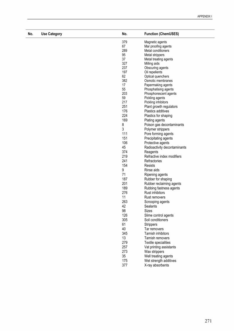
APPENDIX I
271
No. Use Category No. Function (ChemUSES)
379 Magnetic agents67 Mar proofing agents289 Metal conditioners95 Metal strippers37 Metal treating agents327 Milling aids237 Obscuring agents197 Oil repellents62 Optical quenchers382 Osmotic membranes17 Papermaking agents55 Phosphatising agents203 Phosphorescent agents59 Pickling agents217 Pickling inhibitors251 Plant growth regulators176 Plastics additives224 Plastics for shaping169 Plating agents8 Poison gas decontaminants3 Polymer strippers111 Pore forming agents151 Precipitating agents106 Protective agents45 Radioactivity decontaminants374 Reagents219 Refractive index modifiers241 Refractories154 Resists9 Rinse aids71 Ripening agents187 Rubber for shaping201 Rubber reclaiming agents189 Rubbing fastness agents276 Rust inhibitors11 Rust removers263 Scrooping agents42 Sealants98 Sizes126 Slime control agents305 Soil conditioners61 Strippers40 Tar removers345 Tarnish inhibitors13 Tarnish removers279 Textile specialities257 Vat printing assistants273 Wax strippers35 Well treating agents175 Wet strength additives377 X-ray absorbents

APPENDIX I
272
Appendix I-b: List of synonyms for functions according to ChemUSES (US EPA, 1980)
No. ChemUSES Function Use category EU(No.)
104 Abherents 6204 Ablatives 55105 Abrasives 0131 Absorbents 1321 Accelerators 43214 Acidulants 26254 Acoustical insulating material 3246 Activators (chemical
processes)43
163 Activators (ore processing) 23196 Activators (luminescence) 55239 Activators (enzymes) 43110 Adhesion promoters 43302 Adhesives 260 Adsorbents 1354 Aerating agents 0178 Aerosol propellents 347 Air entraining agents 0287 Algicides 39376 Alloying agents 0238 Analytical and product testing 34166 Animal repellents 3863 Antiblocking agents 6188 Anticaking agents 6277 Anticracking agents 4990 Anticratering agents 048 Anticreasing agents 0291 Anticrock agents 214 Antifelting agents 4341 Antifloating agents 50152 Antiflooding agents 52234 Antifogging agents 5099 Antifogging agents 01 Antifouling agents 39329 Antifouling agents 2877 Antifreezes 512 Antifume agents 49129 Antihydrolysis agents 4976 Antiknock agents 28120 Antilivering agents 49, 52230 Antioxidants 14, 49168 Antiozonants 49301 Antiperspirants 15218 Antipilling agents 55282 Antiplasticisers 49177 Antiprecipitants 11293 Antiredeposition agents 9160 Antisagging agents 4964 Antiscaling agents 14119 Antiseize agents 3568 Antisettling agents 49350 Antiskid agents 0343 Antiskinning agents 52352 Antislip finishing agents 43206 Antistaining agents 43328 Antistatic agents 7347 Antistripping agents 21194 Antiwebbing agents 43333 Bactericides 38268 Barrier coating agents 21269 Bates 47143 Binders 2108 Biocides 386 Blasting abrasives 0
132 Bleaching agents 8304 Bleaching assistants 85 Bloom agents 1088 Bloom inhibitors 49358 Blowing agents 2570 Bluing agents 0180 Boil-off assistants 9101 Brazing agents 54220 Bright dips 0353 Brighteners 17281 Builders 43222 Carbonising agents 43164 Carriers 43324 Case-hardening agents 13170 Catalysts 4319 Catalyst supports 4331 Chain extenders 43113 Chain terminators 43141 Chain transfer agents 43122 Chelating agents 34, 42, 43133 Chemical blowing agents 2593 Chemical raw materials 0298 Clarifiers 0242 Cleaners 9260 Cloud point depressants 0114 Coagulants 43278 Coalescents 43357 Coalescing agents 43130 Coating agents 0283 Collectors 086 Colouring agents 10124 Complexing agents 11355 Concrete additives 1372 Coolants 29323 Corrosion inhibitors 14167 Cosmetic ingredients 15123 Coupling agents (polymers) 49174 Coupling agents (dyes) 10335 Coupling agents (solutions) 55315 Crabbing assistants 43228 Crosslinking agents 43215 Culture nutrients 0226 Curing agents (concrete) 43369 Curing agents (polymer
technology)43
18 Currying agents 43366 De-inkers 4381 Deaerating agents 0236 Deasphalting agents 43309 Deblooming agents 085 Dechlorinating agents 5597 Decontaminats 38342 Defoamers 43229 Degreasers 48365 Degumming agents 43137 Dehairing agents 43213 Dehumidifiers 173 Dehydrating agents 0, 3474 Deicers 5107 Deionizers 0, 3484 Delignification agents 43102 Delustrants 31232 Demulsifiers 0200 Denaturants 052 Deodorants 530 Depolymerisation agents 43

APPENDIX I
273
183 Deposit modifiers 28367 Depressants 4349 Descaling agents 0198 Desensitisers (explosives) 42299 Desensitisers (photography) 42292 Desizing agents 43300 Detackifiers 6173 Detergents 9179 Detonators 18182 Developers 42231 Devulcanising agents 47205 Dewatering aids 082 Dewaxing solvents 48356 Discharge printing agents 0140 Disinfectants 39259 Dispersants 4338 Drainage aids 0317 Dryers 4344 Drilling mud additives 0322 Dry strength additives 026 Dust control agents 16233 Dusting agents 6150 Dye carriers 43255 Dye leveling agents 43307 Dye retardants 43211 Dye retention aids 4339 Dye stripping agents 0267 Dyes 1028 Elasticisers 47161 Electrical conductive agents 12311 Electrical insulating material 3289 Electroconductive coating
agents7
383 Electrode materials 12245 Electrolytes 12100 Electron emission agents 0340 Eluting agents 0372 Embalming agents 0361 Embrittlement inhibitors 13265 Emollients 47159 Emulsifiers 49186 Encapsulating agents 057 Enhanced oil recovery agents 0308 Entraining agents 0341 Enzyme inhibitors 43157 Enzymes 43319 Etching agents 0336 Evaporation control agents 0363 Explosion inhibitors 18158 Explosives 18373 Extraction agents 34, 4866 Feed additives 2634 Fertilisers 19207 Fiber-forming compounds 0212 Fillers (patching) 20351 Fillers (augmentation) 20368 Filtration aids 0284 Finishing agents 4325 Fire extinguishing agents 22295 Fixatives 21112 Fixing agents (textile
technology)21
134 Fixing agents (fragrances) 21332 Flame retardants 2256 Flatting agents 079 Flavours and fragrances 0, 36190 Flocculating agents 23297 Flotation agents 23142 Fluid loss additives 020 Fluorescent agents 10
22 Fluxing agents 54145 Food additives 2337 Formation aids 4394 Frothers 25306 Fuel additives 28331 Fuel oxidisers 43247 Fuels 27117 Fulling agents 4332 Fume suppressants 17270 Fumigants 38313 Functional fluids 0, 5, 12, 29, 30, 35362 Fungicides 38221 Gelling agents 52193 Greaseproofing agents 0184 Grinding, lapping, sanding and
polishing abrasives0
99 Heat transfer agents 29314 Heat insulating materials 3287 Heat stabilisers 49275 Herbicides 38192 Hormones 0318 Humectants 7246 Humidity indicators 065 Hydraulic fluids 30210 Hydrotropic agents 0181 Impact modifiers 0380 Incandescent agents 027 Incendiaries 1869 Indicators 0, 34103 Initiators 43146 Inorganic intermediates 33155 Insect attractants 38348 Insect repellents 38330 Insecticides 38162 Insulating materials 32286 Intensifiers (photography) 42359 Intensifiers (printing) 43148 Internal lubricating agents 352 Ion exchange agents 0171 Kier boiling assistants 4391 Lachrymators 0248 Lakes 1033 Latex compounding agents 0172 Laundry sours 4053 Leaching agents 0156 Leather processing agents 0285 Light stabilisers 42370 Liquid crystals 0195 Lubricant additives 35364 Lubricating agents 35381 Luminescent agents 0, 10379 Magnetic agents 067 Mar proofing agents 55375 Materials for shaping 1335 Mercerising assistants 10289 Metal conditioners 037 Metal treating agents 095 Metal strippers 0327 Milling aids 0360 Modifiers 23115 Monomers 33227 Mordents 21252 Nematocides 3824 Nucleating agents 43237 Obscuring agents 0339 Odorants 36197 Oil repellents 0346 Oiliness agents 35128 Opacifiers 1062 Optical quenchers 0
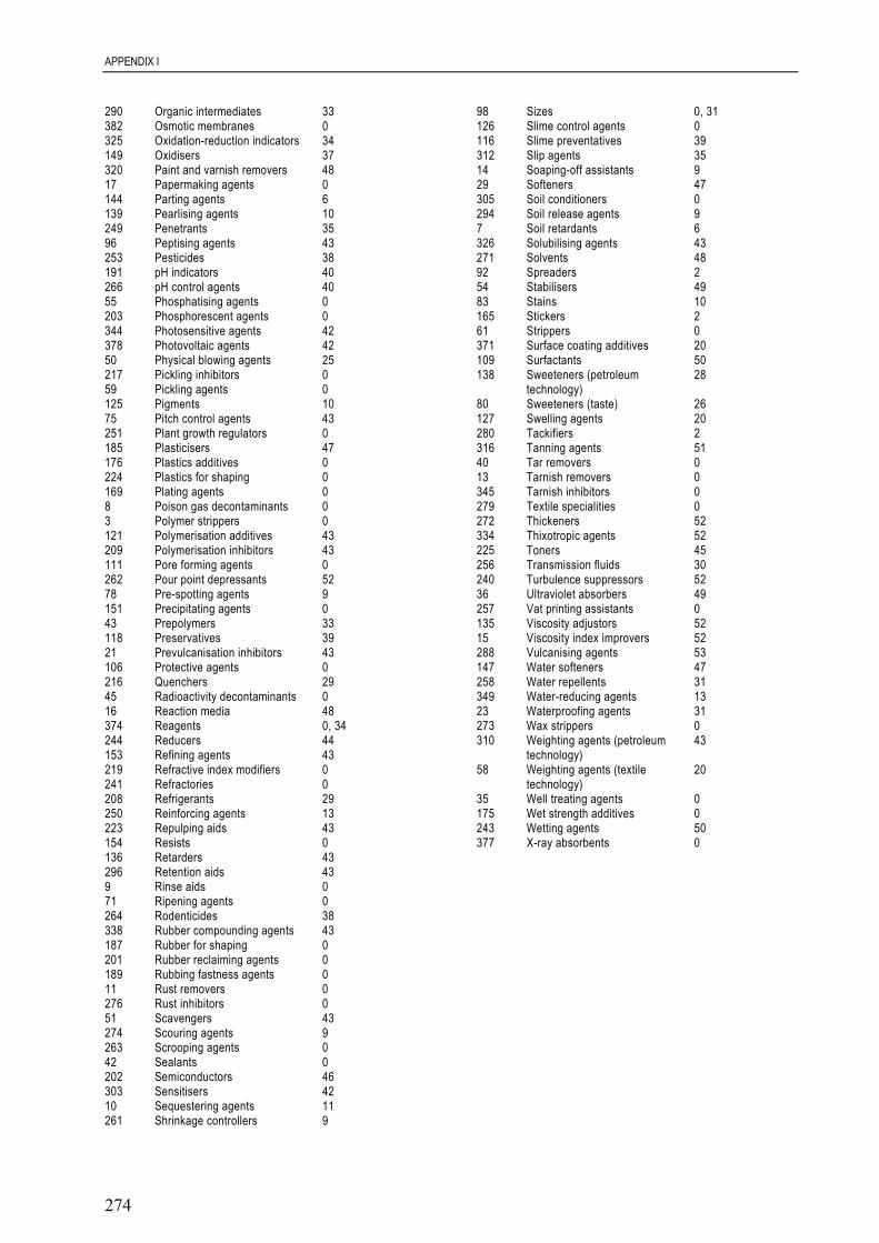
APPENDIX I
274
290 Organic intermediates 33382 Osmotic membranes 0325 Oxidation-reduction indicators 34149 Oxidisers 37320 Paint and varnish removers 4817 Papermaking agents 0144 Parting agents 6139 Pearlising agents 10249 Penetrants 3596 Peptising agents 43253 Pesticides 38191 pH indicators 40266 pH control agents 4055 Phosphatising agents 0203 Phosphorescent agents 0344 Photosensitive agents 42378 Photovoltaic agents 4250 Physical blowing agents 25217 Pickling inhibitors 059 Pickling agents 0125 Pigments 1075 Pitch control agents 43251 Plant growth regulators 0185 Plasticisers 47176 Plastics additives 0224 Plastics for shaping 0169 Plating agents 08 Poison gas decontaminants 03 Polymer strippers 0121 Polymerisation additives 43209 Polymerisation inhibitors 43111 Pore forming agents 0262 Pour point depressants 5278 Pre-spotting agents 9151 Precipitating agents 043 Prepolymers 33118 Preservatives 3921 Prevulcanisation inhibitors 43106 Protective agents 0216 Quenchers 2945 Radioactivity decontaminants 016 Reaction media 48374 Reagents 0, 34244 Reducers 44153 Refining agents 43219 Refractive index modifiers 0241 Refractories 0208 Refrigerants 29250 Reinforcing agents 13223 Repulping aids 43154 Resists 0136 Retarders 43296 Retention aids 439 Rinse aids 071 Ripening agents 0264 Rodenticides 38338 Rubber compounding agents 43187 Rubber for shaping 0201 Rubber reclaiming agents 0189 Rubbing fastness agents 011 Rust removers 0276 Rust inhibitors 051 Scavengers 43274 Scouring agents 9263 Scrooping agents 042 Sealants 0202 Semiconductors 46303 Sensitisers 4210 Sequestering agents 11261 Shrinkage controllers 9
98 Sizes 0, 31126 Slime control agents 0116 Slime preventatives 39312 Slip agents 3514 Soaping-off assistants 929 Softeners 47305 Soil conditioners 0294 Soil release agents 97 Soil retardants 6326 Solubilising agents 43271 Solvents 4892 Spreaders 254 Stabilisers 4983 Stains 10165 Stickers 261 Strippers 0371 Surface coating additives 20109 Surfactants 50138 Sweeteners (petroleum
technology)28
80 Sweeteners (taste) 26127 Swelling agents 20280 Tackifiers 2316 Tanning agents 5140 Tar removers 013 Tarnish removers 0345 Tarnish inhibitors 0279 Textile specialities 0272 Thickeners 52334 Thixotropic agents 52225 Toners 45256 Transmission fluids 30240 Turbulence suppressors 5236 Ultraviolet absorbers 49257 Vat printing assistants 0135 Viscosity adjustors 5215 Viscosity index improvers 52288 Vulcanising agents 53147 Water softeners 47258 Water repellents 31349 Water-reducing agents 1323 Waterproofing agents 31273 Wax strippers 0310 Weighting agents (petroleum
technology)43
58 Weighting agents (textiletechnology)
20
35 Well treating agents 0175 Wet strength additives 0243 Wetting agents 50377 X-ray absorbents 0

APPENDIX I
275
Appendix I-c: Input scheme for emission data on substances
1. Characterisation
Yes NoHigh production volume chemical □ □Other existing chemical □ □New chemical □ □Not specified □
2. Tonnage
A Produced (tpa): □, □ □ □, □ □ □. □ □ □B Imported (tpa): □, □ □ □, □ □ □. □ □ □C Exported (tpa): □, □ □ □, □ □ □. □ □ □
3. Use and stages of the life-cycle
Yes NoProduction □ □
Processing Production Formulation Private use RecoveryNo. Fraction IC UC No Yes No Yes No Yes No Yes No1 □ □ □ 5 □ □ □ □ □ □ □ □ □ □2 □ □ □ □ □ □ □ □ □ □ □ □ □ □ □ □3 □ □ □ □ □ □ □ □ □ □ □ □ □ □ □ □4 □.□ □ □ □ □ □ □ □ □ □ □ □ □ □ □5 □.□ □ □ □ □ □ □ □ □ □ □ □ □ □ □N.B. Private use is specified by IC 5 Personal/Domestic; This is the direct use of the substance (or a formulation containing the substance)
by the public at large.If the processing step has not to be considered at the assessment “No” is marked (not applicable for IC 5).
4. Production characteristics
D Main producer (tpa): □,□ □ □, □ □ □. □ □ □Not specified: □ IC 3, UC 33
Non-isolated intermediate (MC 1a) □Isolated intermediate, stored on site (MC 1b) □Isolated intermediate with controlled transport (MC 1c) □Not specified (MC 1c) □

APPENDIX I
276
Other IC/UC combinations
Continuous production (MC 1b) □Batch process with dedicated equipment (MC 1c) □Batch process with multi-purpose equipment (MC 3) □Not specified (MC 3) □Production capacity of the main source (producer)
E Capacity (t/day) □ □, □ □ □, □ □ □. □ □ □F Period (days/year) □ □, □ □ □, □ □ □. □ □ □Not specified □Specific emission informationEmission G: kg/tonne or Fraction (EFcomp-prod)Air □ □ □. □ □ □ 0. □ □ □Wastewater □ □ □. □ □ □ 0. □ □ □Soil □ □ □. □ □ □ 0. □ □ □Not specified □
5. Formulation characteristics
N.B. For every IC/UC-combination specified in (3) Use and stage of the life-cycle:
Specific information on the scale of formulationOne company (fraction of main source = 1) □Fraction of main source (Fms-form) 0. □ □ □specified □
No specific emission informationDedicated equipment and (very) little cleaningoperations (MC 1b) □Dedicated equipment and frequent cleaning operations (MC 1c) □Multi-purpose equipment (MC 3) □Unknown □
Specific emission informationEmission H: kg/tonne or Fraction (EFcomp-form)Air □ □ □. □ □ □ 0. □ □ □Wastewater □ □ □. □ □ □ 0. □ □ □Soil □ □ □. □ □ □ 0. □ □ □
Content in formulated product
Content: □ □ □. □ □ □ %, or fraction: 0. □ □ □In case of a given range:
Minimum: □ □ □. □ □ □ %, or fraction: 0. □ □ □Maximum: □ □ □. □ □ □ %, or fraction: 0. □ □ □
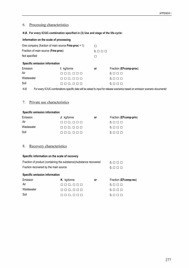
APPENDIX I
277
6. Processing characteristics
N.B. For every IC/UC-combination specified in (3) Use and stage of the life-cycle:
Information on the scale of processing
One company (fraction of main source Fms-proc = 1) □Fraction of main source (Fms-proc) 0. □ □ □Not specified □Specific emission informationEmission I: kg/tonne or Fraction (EFcomp-proc)Air □ □ □. □ □ □ 0. □ □ □Wastewater □ □ □. □ □ □ 0. □ □ □Soil □ □ □. □ □ □ 0. □ □ □N.B. For every IC/UC-combinations specific data will be asked to input for release scenarios based on emission scenario documents!
7. Private use characteristics
Specific emission informationEmission J: kg/tonne or Fraction (EFcomp-priv) Air □ □ □. □ □ □ 0. □ □ □Wastewater □ □ □. □ □ □ 0. □ □ □Soil □ □ □. □ □ □ 0. □ □ □
8. Recovery characteristics
Specific information on the scale of recovery
Fraction of product (containing the substance)/substance recovered 0. □ □ □Fraction recovered by the main source 0. □ □ □Specific emission informationEmission K: kg/tonne or Fraction (EFcomp-rec)Air □ □ □. □ □ □ 0. □ □ □Wastewater □ □ □. □ □ □ 0. □ □ □Soil □ □ □. □ □ □ 0. □ □ □
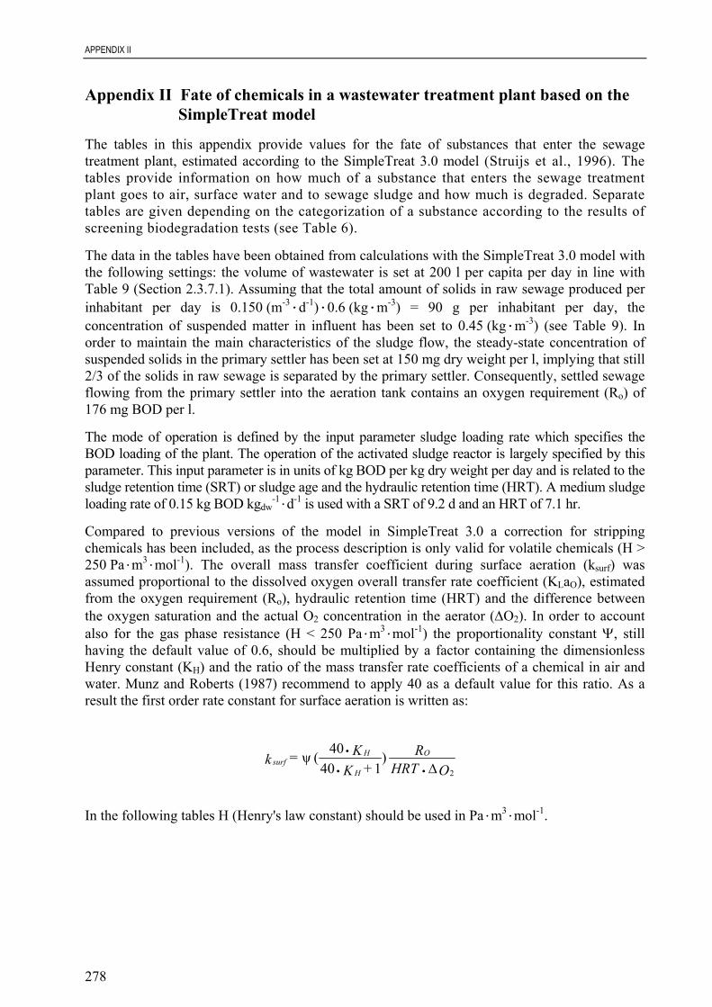
APPENDIX II
278
Appendix II Fate of chemicals in a wastewater treatment plant based on theSimpleTreat model
The tables in this appendix provide values for the fate of substances that enter the sewagetreatment plant, estimated according to the SimpleTreat 3.0 model (Struijs et al., 1996). Thetables provide information on how much of a substance that enters the sewage treatmentplant goes to air, surface water and to sewage sludge and how much is degraded. Separatetables are given depending on the categorization of a substance according to the results ofscreening biodegradation tests (see Table 6).
The data in the tables have been obtained from calculations with the SimpleTreat 3.0 model withthe following settings: the volume of wastewater is set at 200 l per capita per day in line withTable 9 (Section 2.3.7.1). Assuming that the total amount of solids in raw sewage produced perinhabitant per day is 0.150 (m-3.d-1).0.6 (kg.m-3) = 90 g per inhabitant per day, theconcentration of suspended matter in influent has been set to 0.45 (kg.m-3) (see Table 9). Inorder to maintain the main characteristics of the sludge flow, the steady-state concentration ofsuspended solids in the primary settler has been set at 150 mg dry weight per l, implying that still2/3 of the solids in raw sewage is separated by the primary settler. Consequently, settled sewageflowing from the primary settler into the aeration tank contains an oxygen requirement (Ro) of176 mg BOD per l.
The mode of operation is defined by the input parameter sludge loading rate which specifies theBOD loading of the plant. The operation of the activated sludge reactor is largely specified by thisparameter. This input parameter is in units of kg BOD per kg dry weight per day and is related to thesludge retention time (SRT) or sludge age and the hydraulic retention time (HRT). A medium sludgeloading rate of 0.15 kg BOD kgdw
-1.d-1 is used with a SRT of 9.2 d and an HRT of 7.1 hr.
Compared to previous versions of the model in SimpleTreat 3.0 a correction for strippingchemicals has been included, as the process description is only valid for volatile chemicals (H >250 Pa.m3.mol-1). The overall mass transfer coefficient during surface aeration (ksurf) wasassumed proportional to the dissolved oxygen overall transfer rate coefficient (KLaO), estimatedfrom the oxygen requirement (Ro), hydraulic retention time (HRT) and the difference betweenthe oxygen saturation and the actual O2 concentration in the aerator (∆O2). In order to accountalso for the gas phase resistance (H < 250 Pa.m3.mol-1) the proportionality constant Ψ, stillhaving the default value of 0.6, should be multiplied by a factor containing the dimensionlessHenry constant (KH) and the ratio of the mass transfer rate coefficients of a chemical in air andwater. Munz and Roberts (1987) recommend to apply 40 as a default value for this ratio. As aresult the first order rate constant for surface aeration is written as:
In the following tables H (Henry's law constant) should be used in Pa.m3.mol-1.
OHRTR
+ KK = k O
H
Hsurf
2
)140
40( ψ∆••
•

APPENDIX II
279
a) No biodegradability
Fate of chemicals that are not degradable: kbiostp = 0 hr-1 in the aqueous phase of activatedsludge.
log H% to air -4 -3 -2 -1 0 1 2 3 4 5
log Kow 0 0 0 0 0 2 15 64 91 95 951 0 0 0 0 2 15 64 91 95 952 0 0 0 0 2 15 64 91 94 953 0 0 0 0 2 14 62 89 92 924 0 0 0 0 1 12 52 77 80 805 0 0 0 0 1 5 28 48 51 516 0 0 0 0 0 1 9 23 27 27
log H% to water -4 -3 -2 -1 0 1 2 3 4 5
log Kow 0 100 100 100 100 98 85 36 9 5 51 100 100 100 100 98 85 36 9 5 52 99 99 99 99 97 84 36 9 5 53 96 96 96 96 94 82 35 8 5 54 79 79 79 79 77 68 30 8 5 45 39 39 39 39 39 35 19 6 4 46 15 15 15 15 15 14 11 6 4 4
log H% to sludge -4 -3 -2 -1 0 1 2 3 4 5
log Kow 0 0 0 0 0 0 0 0 0 0 01 0 0 0 0 0 0 0 0 0 02 1 1 1 1 1 1 1 0 0 03 4 4 4 4 4 4 3 3 3 34 21 21 21 21 21 20 18 16 15 155 61 61 61 61 60 59 53 46 45 456 85 85 85 85 85 85 80 71 69 69
log H% degraded -4 -3 -2 -1 0 1 2 3 4 5
log Kow 0 0 0 0 0 0 0 0 0 0 01 0 0 0 0 0 0 0 0 0 02 0 0 0 0 0 0 0 0 0 03 0 0 0 0 0 0 0 0 0 04 0 0 0 0 0 0 0 0 0 05 0 0 0 0 0 0 0 0 0 06 0 0 0 0 0 0 0 0 0 0
log H% removal -4 -3 -2 -1 0 1 2 3 4 5
log Kow 0 0 0 0 0 2 15 64 91 95 951 0 0 0 0 2 15 64 91 95 952 1 1 1 1 3 16 64 91 95 953 4 4 4 4 6 18 65 92 95 954 21 21 21 21 23 32 70 92 95 965 61 61 61 61 61 65 81 94 96 966 85 85 85 85 85 86 89 94 96 96

APPENDIX II
280
b) Inherent biodegradability
Fate of chemicals that are “inherently biodegradable” in an OECD/EU test: kbiostp = 0.1 hr-1 inthe aqueous phase of activated sludge.
log H% to air -4 -3 -2 -1 0 1 2 3 4 5
log Kow 0 0 0 0 0 1 10 50 85 91 911 0 0 0 0 1 10 50 85 91 912 0 0 0 0 1 10 50 85 90 913 0 0 0 0 1 9 49 83 88 894 0 0 0 0 1 8 41 72 77 775 0 0 0 0 0 4 23 45 49 496 0 0 0 0 0 1 8 22 26 26
log H% to water -4 -3 -2 -1 0 1 2 3 4 5
log Kow 0 59 59 59 59 58 52 28 8 5 51 59 59 59 59 58 52 28 8 5 52 59 59 59 59 58 52 27 8 5 53 57 57 57 57 56 50 27 8 5 54 48 48 48 48 48 43 24 7 5 45 28 28 28 28 27 25 16 5 4 36 13 13 13 13 13 13 10 6 4 4
log H% to sludge -4 -3 -2 -1 0 1 2 3 4 5
log Kow 0 0 0 0 0 0 0 0 0 0 01 0 0 0 0 0 0 0 0 0 02 1 1 1 1 1 1 1 0 0 03 4 4 4 4 4 4 3 3 3 34 19 19 19 19 19 19 17 16 15 155 56 56 56 56 56 55 51 46 45 456 83 83 83 83 82 82 78 71 69 68
log H% degraded -4 -3 -2 -1 0 1 2 3 4 5
log Kow 0 41 41 41 41 41 38 22 7 4 41 41 41 41 41 40 38 22 7 4 42 41 41 41 41 40 38 22 7 4 43 39 39 39 39 39 37 21 6 4 44 33 33 33 33 32 31 18 6 4 35 17 17 17 17 16 16 10 4 2 26 4 4 4 4 4 4 4 2 1 1
log H% removal -4 -3 -2 -1 0 1 2 3 4 5
log Kow 0 41 41 41 41 42 48 72 92 95 951 41 41 41 41 42 48 72 92 95 952 41 41 41 41 42 48 73 92 95 953 43 43 43 43 44 50 73 92 95 954 52 52 52 52 52 57 76 93 95 965 72 72 72 72 73 75 84 95 96 976 87 87 87 87 87 87 90 94 96 96

APPENDIX II
281
c) pass levels within 28 days in a test on “ready biodegradability”, 10-day window criterionis not fulfilled
Fate of chemicals that reach the biodegradation pass levels within 28 days in an OECD/EU teston “ready biodegradability but not within the 10 day time window: kbiostp = 0.3 hr-1 in theaqueous phase of activated sludge.
log H% to air -4 -3 -2 -1 0 1 2 3 4 5
log Kow 0 0 0 0 0 1 6 36 76 84 851 0 0 0 0 1 6 36 76 84 852 0 0 0 0 1 6 36 75 83 843 0 0 0 0 1 6 35 73 81 824 0 0 0 0 1 5 30 64 71 715 0 0 0 0 0 3 17 40 45 466 0 0 0 0 0 1 7 20 24 25
log H% to water -4 -3 -2 -1 0 1 2 3 4 5
log Kow 0 33 33 33 33 32 29 19 7 5 41 33 33 33 33 32 29 19 7 5 42 32 32 32 32 32 29 19 7 5 43 32 32 32 32 31 29 18 7 5 44 27 27 27 27 27 25 16 6 4 45 18 18 18 18 17 16 12 5 3 36 11 11 11 11 11 10 9 5 4 4
log H% to sludge -4 -3 -2 -1 0 1 2 3 4 5
log Kow 0 0 0 0 0 0 0 0 0 0 01 0 0 0 0 0 0 0 0 0 02 1 1 1 1 1 1 1 0 0 03 3 3 3 3 3 3 3 3 3 34 17 17 17 17 17 17 16 16 15 155 51 51 51 51 51 51 49 46 45 456 79 79 79 79 79 78 76 70 68 68
log H% degraded -4 -3 -2 -1 0 1 2 3 4 5
log Kow 0 67 67 67 67 67 64 45 17 12 111 67 67 67 67 67 64 45 17 12 112 67 67 67 67 67 64 45 17 12 113 65 65 65 65 65 62 44 17 11 114 55 55 55 55 55 53 38 15 10 95 31 31 31 31 31 30 22 9 6 66 11 11 11 11 11 10 9 5 3 3

APPENDIX II
282
log H% removal -4 -3 -2 -1 0 1 2 3 4 5
log Kow 0 67 67 67 67 68 71 81 93 95 961 67 67 67 67 68 71 81 93 95 962 68 68 68 68 68 71 81 93 95 963 68 68 68 68 69 71 82 93 95 964 73 73 73 73 73 75 84 94 96 965 82 82 82 82 83 84 88 95 97 976 89 89 89 89 89 90 91 95 96 96
d) pass levels within 28 days in a test on “ready biodegradability”, 10-day window criterionis fulfilled
Fate of chemicals that are “readily biodegradable” in an OECD/EU test: kbiostp = 1 hr-1 in theaqueous phase of activated sludge.
log H% to air -4 -3 -2 -1 0 1 2 3 4 5
log Kow 0 0 0 0 0 0 3 19 55 66 681 0 0 0 0 0 3 19 55 66 682 0 0 0 0 0 3 19 54 66 673 0 0 0 0 0 3 18 53 64 664 0 0 0 0 0 3 16 46 56 575 0 0 0 0 0 1 9 29 36 376 0 0 0 0 0 1 4 15 20 20
log H% to water -4 -3 -2 -1 0 1 2 3 4 5
log Kow 0 13 13 13 13 13 12 9 5 4 31 13 13 13 13 13 12 9 5 4 32 13 13 13 13 12 12 9 5 4 33 12 12 12 12 12 11 9 5 4 34 11 11 11 11 11 10 8 4 3 35 8 8 8 8 8 7 6 4 3 36 7 7 7 7 7 7 6 4 3 3
log H% to sludge -4 -3 -2 -1 0 1 2 3 4 5
log Kow 0 0 0 0 0 0 0 0 0 0 01 0 0 0 0 0 0 0 0 0 02 0 0 0 0 0 0 0 0 0 03 3 3 3 3 3 3 3 3 3 34 16 16 16 16 16 16 16 15 15 155 47 47 47 47 47 47 46 45 45 456 72 72 72 72 72 72 71 69 67 67

APPENDIX II
283
log H% degraded -4 -3 -2 -1 0 1 2 3 4 5
log Kow 0 87 87 87 87 87 85 72 41 30 291 87 87 87 87 87 85 72 40 30 292 87 87 87 87 87 85 72 40 30 293 85 85 85 85 84 82 70 39 29 284 73 73 73 73 73 71 61 34 26 245 45 45 45 45 45 44 38 22 17 166 21 21 21 21 21 21 19 12 9 9
log H% removal -4 -3 -2 -1 0 1 2 3 4 5
log Kow 0 87 87 87 87 87 88 91 95 96 971 87 87 87 87 87 88 91 95 96 972 87 87 87 87 88 88 91 95 96 973 88 88 88 88 88 89 91 95 96 974 89 89 89 89 89 90 92 96 97 975 92 92 92 92 92 93 94 96 97 976 93 93 93 93 93 93 94 96 97 97

APPENDIX III
284
Appendix III Evaluation of data
In determining whether or not the data to be used in the risk assessment are adequate, theirquality and representativeness needs to be evaluated. For this, a number of factors will beconsidered and the test design will be evaluated to ensure that the quality criteria demanded bystandardised tests have in part or in whole been met. Such quality criteria can be detailed ingeneral terms but expert judgement will be required for each substance and test data on a case-by-case basis. A number of papers address the issue of data quality (e.g. SIDS Manual(OECD, 1994a); AQUIRE-database-manual; Tema Nord, 1994). Care should be taken thatthe guidance given is appropriate for the use of data. The following factors should be takeninto account when evaluating the data (on aquatic toxicity):
Identity of the test substance
It is important that the substance tested be properly identified and any significant impuritiesdescribed. Ideally, this should be through the quoting of a CAS No. or other substance specificmeans but the substance name may often be sufficient. However, tests conducted on“dichloro......” when the substance being evaluated is “1,3-dichloro.....” may thus be insufficientto determine exactly what substance was tested. Equally, the presence or absence of a significanttoxic impurity may affect the measured toxicity. Where such an impurity is identified in thesubstance under evaluation, due care should be taken to ensure that its effects are fully taken intoaccount.
Test organisms
Detailed information of the taxonomic identity of aquatic organisms tested should be supplied, toinclude the genus and species. While tests on “non-standard” organisms can be accepted, careshould be taken to ensure that they are properly characterised and the test system appropriate.The animals should be of relatively uniform age, weight and size and should be healthy at thestart of test as shown by low mortality/effects in controls.
Test design
The test system should be adequately described and be considered appropriate for the substanceof concern and organisms tested. The delivery of the test substance should be ensure a controlledand known exposure and the supply of oxygen, food and light be suitable to reduce unnecessarystress in the test organisms. The temperature, pH and water hardness should be recorded and beappropriate for the organisms tested. The number of organisms exposed and number of exposureconcentrations chosen should be sufficient for a valid statistical calculation of the appropriateeffects concentrations to be made.
• the delivery of the test substance represents a critical stage in ensuring adequate exposure ofthe test organisms. When considering the delivery system, due account should be taken ofthe relevant phys. chem. properties of the test substance and their potential effects on thedelivery and exposure systems. For Daphnia and algae static tests are normally used but forfish static, semi-static or flow-through tests may be appropriate. The precise mechanismused to deliver the test substance must therefore be described;
• the exposure concentration should be known and maintained under control (>80% of initialconcentrations) throughout the test. Ideally, the concentrations should be directly measuredat appropriate stages over the course of the test. In many cases, measured concentrations will

APPENDIX III
285
not be available and expert judgement will be necessary to decide whether the exposure ofthe aquatic organisms is adequately described. Such non-measured concentrations arenormally described as 'nominal' concentrations and refer to the level at which it wasintended that exposure would occur. Such concentrations may be acceptable if the testsubstance:
- is sufficient soluble in test water, i.e. the test concentrations are below the watersolubility;
- is relatively stable in test water;- has a low absorbance to the system delivery and exposure apparatus;- is non-volatile.
For the interpretation of data that were generated by using solubilisers the alteredbioavailability (enhancement/reduction) has to be considered. For many substances,including poorly water soluble substances, volatile substances and substances that hydrolyseor adsorb on surfaces, nominal concentrations are often not appropriate and additionalinformation may be necessary in order to verify the actual exposure concentrations. In somecases, the choice of a semi-static or flow-through system (fish test) may allow a presumptionof a stable exposure concentration. In general, the more likely it is that the physical chemicalproperties of the substance would lead to a loss of concentration over the course of the test,the more important it becomes to verify the concentration by direct analysis of the test waterat suitable points throughout the test. Where the exposure concentration can not bedetermined with confidence, the test should be regarded as ' not-valid' for the purposes orrisk assessment;
• The environmental conditions which exist during the test should be recorded and be bothstable and appropriate. Significant variations in the environmental conditions such as pH,temperature, water hardness, oxygen levels and light regime can induce undue stress withinthe test organisms and hence false levels of toxicity. Absence of information on theseparameters would suggest that the test system was not well described although would notnecessary invalidate the data if other quality criteria are met;
• The L(E)C50 would normally be determined on a statistical basis from the effects observedover a range of concentrations. It is important, therefore, that sufficient organisms are testedat each concentration level and sufficient concentration levels are chosen so as to allow astatistically valid derivation to be made of the appropriate effect concentration. In theabsence of this details, a clear indication of the method used to calculate the effect (or noeffect) concentration may be sufficient. Limit tests would not normally be acceptable expectas a means of demonstrating no toxic effects;
• At issue is whether the duration of a standard toxicity test(s) is long enough for thecompound to reach steady state and elicit a toxic response (Hawker and Connell, 1985;Connell, 1990; Kristensen and Tyle 1990). For many organic non-metabolizablecompounds, the time to reach respectively 80% and 95% of the steady state concentration isdepending on lipophilicity of the compound (OECD, 1994b).
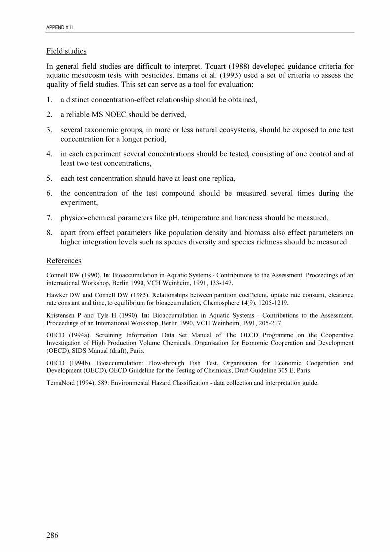
APPENDIX III
286
Field studies
In general field studies are difficult to interpret. Touart (1988) developed guidance criteria foraquatic mesocosm tests with pesticides. Emans et al. (1993) used a set of criteria to assess thequality of field studies. This set can serve as a tool for evaluation:
1. a distinct concentration-effect relationship should be obtained,
2. a reliable MS NOEC should be derived,
3. several taxonomic groups, in more or less natural ecosystems, should be exposed to one testconcentration for a longer period,
4. in each experiment several concentrations should be tested, consisting of one control and atleast two test concentrations,
5. each test concentration should have at least one replica,
6. the concentration of the test compound should be measured several times during theexperiment,
7. physico-chemical parameters like pH, temperature and hardness should be measured,
8. apart from effect parameters like population density and biomass also effect parameters onhigher integration levels such as species diversity and species richness should be measured.
References
Connell DW (1990). In: Bioaccumulation in Aquatic Systems - Contributions to the Assessment. Proceedings of aninternational Workshop, Berlin 1990, VCH Weinheim, 1991, 133-147.
Hawker DW and Connell DW (1985). Relationships between partition coefficient, uptake rate constant, clearancerate constant and time, to equilibrium for bioaccumulation, Chemosphere 14(9), 1205-1219.
Kristensen P and Tyle H (1990). In: Bioaccumulation in Aquatic Systems - Contributions to the Assessment.Proceedings of an International Workshop, Berlin 1990, VCH Weinheim, 1991, 205-217.
OECD (1994a). Screening Information Data Set Manual of The OECD Programme on the CooperativeInvestigation of High Production Volume Chemicals. Organisation for Economic Cooperation and Development(OECD), SIDS Manual (draft), Paris.
OECD (1994b). Bioaccumulation: Flow-through Fish Test. Organisation for Economic Cooperation andDevelopment (OECD), OECD Guideline for the Testing of Chemicals, Draft Guideline 305 E, Paris.
TemaNord (1994). 589: Environmental Hazard Classification - data collection and interpretation guide.

APPENDIX IV
287
Appendix IV Assignment of organisms to trophic levels
Organisms used in ecotoxicological tests can be assigned to different trophic levels, taxonomicgroups, life forms (e.g. sessil, planktonic or swimming), and feeding strategies (e.g. autotrophic,carnivorous, herbivorous, detritivorous, scavengers, omnivorous, deposit or filter feeders.) Theseassignments are related to differences in morphology, behaviour, and physiology, including theirability to take up, metabolise and excrete chemicals. Furthermore, these assignments may also tosome extent determine the likelihood, extent and way the organisms may be exposed. Taken
Primary producers Primary producers photo-/chemo-autotrophically synthesise organic compounds using inorganic precursors. They include: - chlorophyll-containing species of vascular plants - algae, (e.g. green algae: Selenastrum, Scenedesmus, Chlorella; blue-green algae:
Microcystis) - purple sulphur bacteria, chlorobacteria - chemoautotrophic bacteria (nitrifying bacteria, sulphur bacteria). Primary consumers They live mainly on living or dead autotrophic organisms or on microorganisms. Representatives of this trophic level are especially plant-eating animals (i.e. species that are not carnivorous of the following taxonomic groups): - protozoa (e.g. Uronema, Entosiphon, Tetrahymena) - annelida (e.g. Tubifex, Enchytraeus) - crustacea (e.g. Artemia, Daphnia spec., Copepoda, Gammarus, Asellus) - molluscs (e.g. Dreissena, Mytilus, Ostrea; several gastropods: Patella, Viviparus) - insects (some insect larvae that are not carnivorous) - nematoda (those species which are living in water) Secondary consumers They live mainly on primary consumers. Among them are: - predatory insects and larvae of insects (e.g. Chaoborus) - carnivorous protozoa - rotatoria - coelenterata (e.g. Hydra) - predatory copepods - fish (Teleostei: e.g. Cyprinus carpio, Brachydanio rerio, Poecilia reticulata, Oryzias
latipes, Pimephales promelas, Lepomis macrochirus, Oncorhynchus mykiss (previously: Salmo gairdneri, Leuciscus idus melanotus, Cyprinodon, Carassius)
- amphibians (e.g. Rana, Xenopus) Decomposers Organisms of this trophic level break down dead organic material to inorganic constitu-ents. Standard organisms are underlined

APPENDIX IV
288
together the mentioned differences may explain the observed variability among organismsregarding their sensitivity to the toxicity of chemicals, even though it may be difficult orimpossible to attribute which differences between two organisms are the actual reason for theirsensitivity to a certain toxic chemical.
The standard organisms which are usually used in standard tests (plankton micro-algae, Daphniaand fish) represent three trophic levels (primary producers, primary consumers and secondaryconsumers), three taxonomic groups (green algae, crustaceans and bone fish), two life forms(plankton or nekton) and three feeding strategies (photosynthetic, herbivorous filter feeder andcarnivorous).
Accordingly, non-standard organisms can be assigned to equivalent trophic levels, taxonomicgroups etc.
The assignment of an organism to a trophic level is based on the energy balance of theecosystem concerned and is not primarily dependent on the species. Therefore, a givenpopulation may represent more than one trophic level depending on the spectrum and amount ofnutrition for the species. In addition, earlier life stages may live on completely different nutritioncompared to adults of the same species.

APPENDIX V
289
Appendix V Examples of assays suitable for further testing for soil organisms
Soil organisms
A few suitable test species belonging to additional taxonomic groups were identified in theSERAS-Workshop in 1992 (Soil Ecotoxicological Risk Assessment System). Van Straalen andVan Gestel (1992), Stavola (1990) and Samsøe-Petersen and Pedersen (1994) discuss a numberof terrestrial species and test methods with various degrees of standardisation. Léon and VanGestel (1994) give possible criteria for the evaluation of individual tests and for the selection ofstandardised laboratory toxicity tests with terrestrial organisms.
Results obtained in tests carried out in accordance with guidelines for pesticides may pose aproblem. Only tests where the test substance is applied to the soil in a comparable way to theexposure of existing chemicals can be used for the concentration-effect assessment. Followingrecognition of the lack of standardised soil tests, research programmes have been initiated inSweden (MATS = MArk Test System), in the Netherlands (NISRP = Netherlands Integrated SoilResearch Programme) and in Denmark.
A co-ordinated programme for the development and standardisation of a number of soil testspecies and test systems has also been initiated. This project SECOFASE (Sub-lethal Effects ofChemicals On FAuna Soil Ecosystem) is described by Løkke and Van Gestel (1993, cited inSamsøe-Petersen and Pedersen (1994)). It should be noted that the guideline for a long-term testwith vascular plants has still to be finalised (e.g. with Arabidopsis thaliana or Brassica rapa,Stavola (1990)). Long-term tests for the earth- and compost worms (ISO draft, 1993; DutchDraft Guideline; German Draft Guideline), and the test on Enchytraeids, OECD new guideline220, draft March 2000), and the spring-tail (Dutch Draft Guideline; German Draft; BBA 1990b)are available. These tests analyse effects on reproduction. In addition, the standardisation of thelong-term test on Staphylinids (Coleoptera), where degree of parasitism, hatching rate andreproduction are assessed, is close to completion (Samsøe-Petersen, 1987; Naton, 1989; SETAC,1995).
For biocidal active substances, the Technical Notes for Guidance on data requirements insupport to Directive 98/8/EC proposes guidance to the additional data requirements in casefurther testing are necessary after the results of the ecotoxicological studies submitted in thecommon core data set and the intended use(s) of the active substance, as well as further testingstrategies for evaluating the fate and behaviour in the environment of the active substancetogether with its transformation products and their ecotoxicological effects (TNsG on DataRequirements, 2000).

APPENDIX V
290
Table 1 Selected soil test methodologies
Test Organism Duration Endpoints Reference/Source Comments
Microbial Processes
Microbial Processes
N-Transformation≥28 d M (i) EU draft C.21: Soil Microorganisms. Nitrification
Transformation Test.(ii) OECD 216 Soil Microorganisms, Nitrogen TransformationTest (2000).(iii) ISO 14238 Soil quality – Biological methods:Determination of nitrogen mineralisation and nitrification insoils and the influence of chemicals on these processes(1997).
− Addresses short-term adverse effects.− Based on soil microflora nitrate production.− Bacteria are present at up to 10 million per cm2 in soils. This
corresponds to several tonnes per hectare.
Microbial Processes
C-Transformation≥28 d M (i) EU draft C.22: Soil Microorganisms. Carbon Transformation
Test.(ii) OECD 217 Soil Microorganisms, Carbon TransformationTest (2000).(iii) ISO 14238 Soil quality – Laboratory incubations systemsfor measuring the mineralisation of organic chemicals in soilunder aerobic conditions (1997).
− Addresses short-term adverse effects.− Based on soil microflora respiration rate.− Bacteria are present at up to 10 million per cm2 in soils. This
corresponds to several tonnes per hectare.
Invertebrate Fauna
Eisenia fetida/andrei
(Oligochaeta)
7 – 14 d S (i) EU C.8: Earthworm acute toxicity test.(ii) OECD 207 Earthworm acute toxicity tests (1984).(iii) ISO 11268-1 Soil Quality – Effects of pollutants onearthworms (Eisenia fetida). Part 1: Determination of acutetoxicity using artificial soil substrate (1993).(iv) ASTM E1676-97 Standard guide for conducting laboratorysoil toxicity or bioaccumulation tests with the Lumbricidearthworm Eisenia fetida (1997).
− Adult survival assessed after 1 – 2 weeks.− Important ecological function (enhance decomposition and
mineralisation via incorporation of matter into soil).− Important food source and potential route of bioaccumulation by
higher organisms.− Large size/ease of handling.− Readily cultured/maintained in the laboratory.− Litter-dwelling epigeic species.− Standard test organism for terrestrial ecotoxicology.− The Lumbricidae account for 12% of the edaphon (soil biota) by
biomass and are therefore important prey species.
Table 1 continued overleaf

APPENDIX V
291
Table 1 continued Selected soil test methodologies
Test Organism Duration Endpoints Reference/Source Comments
Invertebrate Fauna (continued)
Eisenia fetida/andrei
(Oligochaeta)
28d + 28d S/G/R (i) OECD (2000). Earthworm Reproduction Test (Draft).(ii) ISO 11268-2 Soil Quality – Effects of Pollutants onEarthworms (Eisenia fetida). Part 2: Determination of Effectson Reproduction (1998).(iii) US EPA (1996). Ecological Effects Test Guidelines.OPPTS 850.6200 Earthworm Subchronic Toxicity Test.US EPA, Prevention, Pesticides and Toxic Substances (7104).EPA712-C-96-167, April 1996.(iv) Kula & Larink (1998). Tests on the earthworms Eiseniafetida and Aporrectodea caliginosa. In Handbook of SoilInvertebrates (Eds. Hans Løkke & Cornelis A.M. Van Gestel).John Wiley & Sons: Chichester, UK.
− Adult growth and survival assessed after 4 weeks.− Reproduction (juvenile number) assessed after a further 4 weeks (8
weeks total).− Relatively long generation time (8 weeks).− Important ecological function (enhance decomposition and
mineralisation via incorporation of matter into soil).
− Important food source and potential route of bioaccumulation byhigher organisms.
− Large size/ease of handling.− Readily cultured/maintained in the laboratory.− Litter-dwelling epigeic species.− Standard test organism for terrestrial ecotoxicology.− The Lumbricidae account for 12% of the edaphon (soil biota) by
biomass and are therefore important prey species.
Aporrectodeacaliginosa(Oligochaeta)
S/G/R Kula & Larink (1998). Tests on the earthworms Eisenia fetidaand Aporrectodea caliginosa. In Handbook of SoilInvertebrates (Eds. Hans Løkke & Cornelis A.M. Van Gestel).John Wiley & Sons: Chichester, UK.
− Mortality, growth and cocoon number assessed after 4 weeks.− Relatively slow reproductive cycle.− Cultures difficult to maintain.− Horizontal burrowing (endogeic) mineral soil species.− Selective feeders digesting fungi, bacteria and algae.− Dominant in agro-ecosystems. Present at 10 – 250 per m2.
Table 1 continued overleaf

APPENDIX V
292 Table 1 continued Selected soil test methodologies
Test Organism Duration Endpoints Reference/Source Comments
Invertebrate Fauna (continued)
Enchytraeus albidus(Oligochaeta)
21 - 42d S/R (i) OECD (2000). OECD 220 Enchytraeidae Reproduction Test(Draft).(ii) ISO/CD 16387 Soil quality - Effects of soil pollutants onenchytraeids: Determination of effects on reproduction (draft).
− Adult mortality is assessed after 3 weeks.− Reproduction (juvenile number) is assessed after a further 3 weeks
(6 weeks total).− Shorter generation time than earthworms.− Ease of handling/culture.− Enchytraeidae feed on decomposing plant material and associated
microorganisms i.e., fungi, bacteria & algae.− Enchytraeids are abundant in many soil types including those from
which earthworms are often absent. They account for approximately0.5% of the edaphon (soil biota) by mass (up to 50 g per m2). Thiscorresponds to approximately 100,000 per m2.
Cognettiasphagnetorum(Oligochaeta)
70 d G/R Rundgren & Augustsson (1998). Test on the EnchytraeidCognettia sphagnetorum. In Handbook of Soil Invertebrates(Eds. Hans Løkke & Cornelis A.M. Van Gestel). John Wiley &Sons: Chichester, UK.
− Mortality and asexual reproduction (fragmentation rate of adults)determined weekly over 10 weeks.
− Easy to culture.
− Enchytraeidae feed on decomposing plant material and associatedmicroorganisms i.e., fungi, bacteria & algae.
− C. spagnetorum is common in bogs, forests and other highly organichabitats. They are present at 10,000 – 25,000 per m2.
Folsomia candida(Collembola)
28d S/R ISO 11267 Soil Quality – Inhibition of reproduction ofCollembola (Folsomia candida) (1999).
− Survival and reproduction after 4 weeks.− Short generation time.− Ease of culture.− Springtails are important soil litter arthropods playing a role in soil
organic matter breakdown and nutrients recycling.− Feed on bacteria and fungi.− Collembola are the most abundant soil fauna present at 40,000 to
70,000 per m2. Prey for epigeic invertebrates such as mites,centipedes, spiders and carabid beetles.
Table 1 continued overleaf
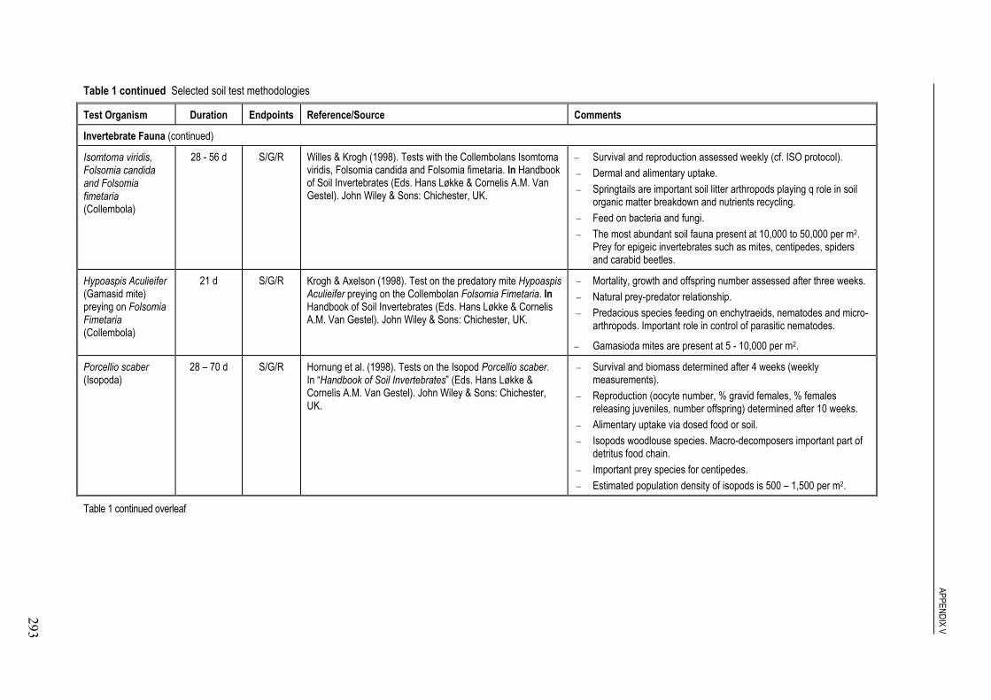
APPENDIX V
293
Table 1 continued Selected soil test methodologies
Test Organism Duration Endpoints Reference/Source Comments
Invertebrate Fauna (continued)
Isomtoma viridis,Folsomia candidaand Folsomiafimetaria(Collembola)
28 - 56 d S/G/R Willes & Krogh (1998). Tests with the Collembolans Isomtomaviridis, Folsomia candida and Folsomia fimetaria. In Handbookof Soil Invertebrates (Eds. Hans Løkke & Cornelis A.M. VanGestel). John Wiley & Sons: Chichester, UK.
− Survival and reproduction assessed weekly (cf. ISO protocol).− Dermal and alimentary uptake.− Springtails are important soil litter arthropods playing q role in soil
organic matter breakdown and nutrients recycling.− Feed on bacteria and fungi.− The most abundant soil fauna present at 10,000 to 50,000 per m2.
Prey for epigeic invertebrates such as mites, centipedes, spidersand carabid beetles.
Hypoaspis Aculieifer(Gamasid mite)preying on FolsomiaFimetaria(Collembola)
21 d S/G/R Krogh & Axelson (1998). Test on the predatory mite HypoaspisAculieifer preying on the Collembolan Folsomia Fimetaria. InHandbook of Soil Invertebrates (Eds. Hans Løkke & CornelisA.M. Van Gestel). John Wiley & Sons: Chichester, UK.
− Mortality, growth and offspring number assessed after three weeks.− Natural prey-predator relationship.− Predacious species feeding on enchytraeids, nematodes and micro-
arthropods. Important role in control of parasitic nematodes.
− Gamasioda mites are present at 5 - 10,000 per m2.
Porcellio scaber(Isopoda)
28 – 70 d S/G/R Hornung et al. (1998). Tests on the Isopod Porcellio scaber.In “Handbook of Soil Invertebrates” (Eds. Hans Løkke &Cornelis A.M. Van Gestel). John Wiley & Sons: Chichester,UK.
− Survival and biomass determined after 4 weeks (weeklymeasurements).
− Reproduction (oocyte number, % gravid females, % femalesreleasing juveniles, number offspring) determined after 10 weeks.
− Alimentary uptake via dosed food or soil.− Isopods woodlouse species. Macro-decomposers important part of
detritus food chain.− Important prey species for centipedes.− Estimated population density of isopods is 500 – 1,500 per m2.
Table 1 continued overleaf

APPENDIX V
294 Table 1 continued Selected soil test methodologies
Test Organism Duration Endpoints Reference/Source Comments
Invertebrate Fauna (continued)
Brachydesmussuperus (Diplopoda)
70 d S/R Tajovsky (1998). Test on the Millipede Brachydesmussuperus. In “Handbook of Soil Invertebrates” (Eds. HansLøkke & Cornelis A.M. Van Gestel). John Wiley & Sons:Chichester, UK.
− Animal number, nest number, egg number and offspring numberdetermined weekly.
− Difficult to maintain culture throughout year.− Alimentary uptake via dosed food or soil.− Millipedes are important primary decomposers of leaf litter and
organic detritus.− Their faecal pellets provide a micro-environment for microorganisms
such as fungi and micro-arthropods.− Important prey for carabid beetles, centipedes and spiders and
insectivorous birds and mammals. Diplopoda are present at 10 –100 per m2.
Lithobius mutabilis(Chilopoda)
28 – 84 d S/G/L/M Laskowski et al. (1998). Test on the Centipede Lithobiusmutabilis. In “Handbook of Soil Invertebrates” (Eds. HansLøkke & Cornelis A.M. Van Gestel). John Wiley & Sons:Chichester, UK.
− Mortality, biomass, respiration rate and locomotor activitydetermined after 4 weeks (degradable compounds) to 12 weeks(persistent compounds).
− Food chain effect measured via use of dosed prey (fly larvae).− Centipedes are important carnivorous arthropods feeding on small
earthworms, millipedes, woodlice and springtails. They are in turnprey for birds and mammals. Chilopoda are present up to 100 perm2.
Philonthus cognatus(Coleoptera)
42 – 70 d S/R Metge & Heimbach (1998). Test on the Staphylinid Philonthuscognatus. In “Handbook of Soil Invertebrates” (Eds. HansLøkke & Cornelis A.M. Van Gestel). John Wiley & Sons:Chichester, UK.
− Beetles exposed for one week to determine subsequent effect onegg production and hatching rate over 6 – 10 weeks. Mortality mayalso be assessed.
− Predators of springtails, aphids, dipterans & coleopteran larvae.Prey to birds, mice and large arthropods.
− Estimated densities of 1 adult per 2 – 5 m2.
Table 1 continued overleaf
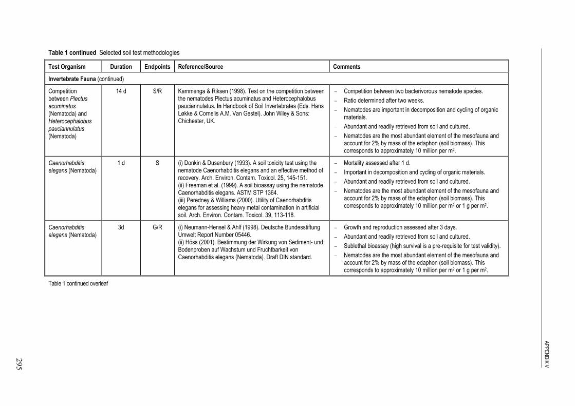
APPENDIX V
295
Table 1 continued Selected soil test methodologies
Test Organism Duration Endpoints Reference/Source Comments
Invertebrate Fauna (continued)
Competitionbetween Plectusacuminatus(Nematoda) andHeterocephalobuspauciannulatus(Nematoda)
14 d S/R Kammenga & Riksen (1998). Test on the competition betweenthe nematodes Plectus acuminatus and Heterocephalobuspauciannulatus. In Handbook of Soil Invertebrates (Eds. HansLøkke & Cornelis A.M. Van Gestel). John Wiley & Sons:Chichester, UK.
− Competition between two bacterivorous nematode species.− Ratio determined after two weeks.− Nematodes are important in decomposition and cycling of organic
materials.− Abundant and readily retrieved from soil and cultured.− Nematodes are the most abundant element of the mesofauna and
account for 2% by mass of the edaphon (soil biomass). Thiscorresponds to approximately 10 million per m2.
Caenorhabditiselegans (Nematoda)
1 d S (i) Donkin & Dusenbury (1993). A soil toxicity test using thenematode Caenorhabditis elegans and an effective method ofrecovery. Arch. Environ. Contam. Toxicol. 25, 145-151.(ii) Freeman et al. (1999). A soil bioassay using the nematodeCaenorhabditis elegans. ASTM STP 1364.(iii) Peredney & Williams (2000). Utility of Caenorhabditiselegans for assessing heavy metal contamination in artificialsoil. Arch. Environ. Contam. Toxicol. 39, 113-118.
− Mortality assessed after 1 d.− Important in decomposition and cycling of organic materials.− Abundant and readily retrieved from soil and cultured.− Nematodes are the most abundant element of the mesofauna and
account for 2% by mass of the edaphon (soil biomass). Thiscorresponds to approximately 10 million per m2 or 1 g per m2.
Caenorhabditiselegans (Nematoda)
3d G/R (i) Neumann-Hensel & Ahlf (1998). Deutsche BundesstiftungUmwelt Report Number 05446.(ii) Höss (2001). Bestimmung der Wirkung von Sediment- undBodenproben auf Wachstum und Fruchtbarkeit vonCaenorhabditis elegans (Nematoda). Draft DIN standard.
− Growth and reproduction assessed after 3 days.− Abundant and readily retrieved from soil and cultured.− Sublethal bioassay (high survival is a pre-requisite for test validity).− Nematodes are the most abundant element of the mesofauna and
account for 2% by mass of the edaphon (soil biomass). Thiscorresponds to approximately 10 million per m2 or 1 g per m2.
Table 1 continued overleaf

APPENDIX V
296 Table 1 continued Selected soil test methodologies
Test Organism Duration Endpoints Reference/Source Comments
Primary Producers
Many test speciesincluding grass
crops(monocotyledonae -
Gramineae),Brassica spp.
(Dicotyledonae –Cruciferae) and
bean crops(Dicotyledonae –
Leguminosae)
5d or 14 – 21d
E/G (i) OECD (2000). OECD 208A Seedling emergence andseedling growth test & OECD 208B: Vegetative vigour test(draft).(ii) ISO 11269-1: Soil quality – Determination of the effects ofpollutants on soil flora – Part 1: Method for the measurementof inhibition of root growth (1993).(iii) ISO 11269-2 Soil quality – Determination of the effects ofpollutants on soil flora – Part 2: Effects of chemicals on theemergence and growth of higher plants (1995).(iv) ASTM E1963-98 Standard guide for conducting terrestrialplant toxicity tests (1998).
− Seed emergence (E) & early life stages of growth (G) in treated soils(208A)
− Vegetative vigour (G) following foliar application (208B).− Root growth of pre-germinated seeds (ISO 11269-1).− Minimum of three test species: one monocotyledon and two
dicotyledon (OECD 208, )
Key: S = survival; E = emergence; G = growth; R = reproduction; M = metabolism; L = locomotory activity

APPENDIX VI
297
Appendix VI Examples of assays suitable for futher testing for sedimentorganisms
In the table selected freshwater sediment toxicity test methods are presented (adapted fromSETAC, 1993). Further sediment tests, e.g. for marine species, can be found in OECD (1998a).
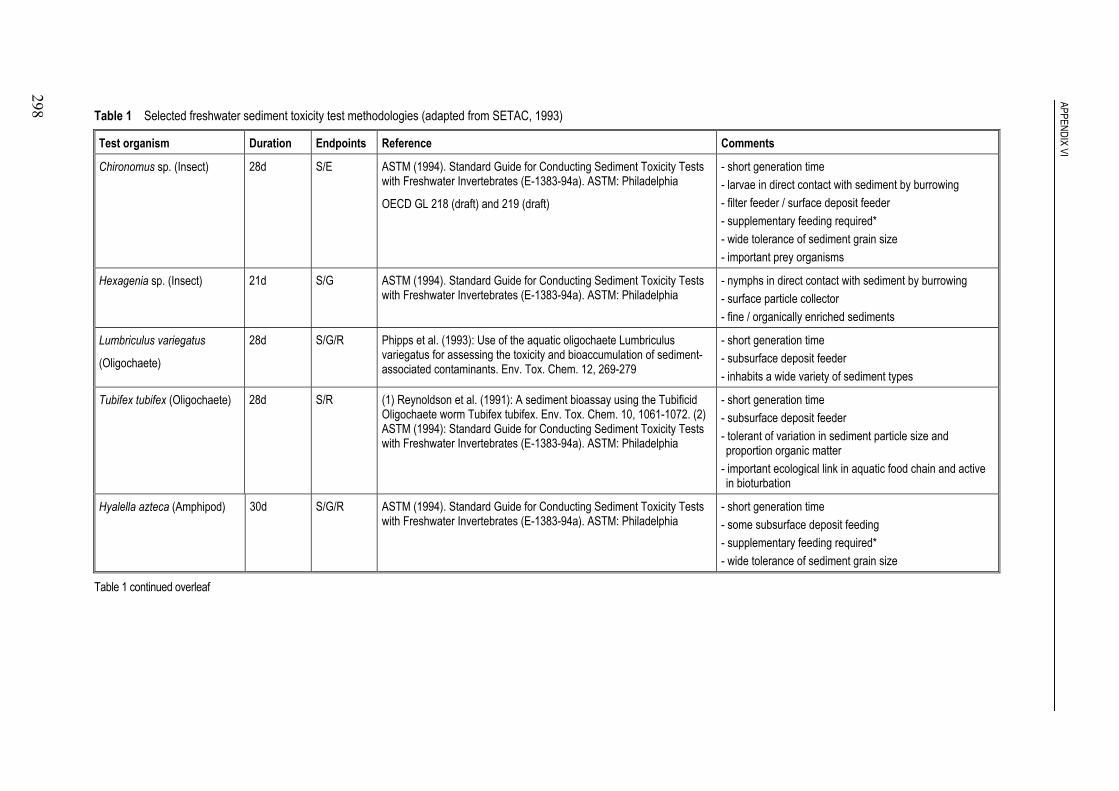
APPENDIX VI
298
Table 1 Selected freshwater sediment toxicity test methodologies (adapted from SETAC, 1993)
Test organism Duration Endpoints Reference Comments
Chironomus sp. (Insect) 28d S/E ASTM (1994). Standard Guide for Conducting Sediment Toxicity Testswith Freshwater Invertebrates (E-1383-94a). ASTM: Philadelphia
OECD GL 218 (draft) and 219 (draft)
- short generation time- larvae in direct contact with sediment by burrowing- filter feeder / surface deposit feeder- supplementary feeding required*- wide tolerance of sediment grain size- important prey organisms
Hexagenia sp. (Insect) 21d S/G ASTM (1994). Standard Guide for Conducting Sediment Toxicity Testswith Freshwater Invertebrates (E-1383-94a). ASTM: Philadelphia
- nymphs in direct contact with sediment by burrowing- surface particle collector- fine / organically enriched sediments
Lumbriculus variegatus
(Oligochaete)
28d S/G/R Phipps et al. (1993): Use of the aquatic oligochaete Lumbriculusvariegatus for assessing the toxicity and bioaccumulation of sediment-associated contaminants. Env. Tox. Chem. 12, 269-279
- short generation time- subsurface deposit feeder- inhabits a wide variety of sediment types
Tubifex tubifex (Oligochaete) 28d S/R (1) Reynoldson et al. (1991): A sediment bioassay using the TubificidOligochaete worm Tubifex tubifex. Env. Tox. Chem. 10, 1061-1072. (2)ASTM (1994): Standard Guide for Conducting Sediment Toxicity Testswith Freshwater Invertebrates (E-1383-94a). ASTM: Philadelphia
- short generation time- subsurface deposit feeder- tolerant of variation in sediment particle size andproportion organic matter
- important ecological link in aquatic food chain and activein bioturbation
Hyalella azteca (Amphipod) 30d S/G/R ASTM (1994). Standard Guide for Conducting Sediment Toxicity Testswith Freshwater Invertebrates (E-1383-94a). ASTM: Philadelphia
- short generation time- some subsurface deposit feeding- supplementary feeding required*- wide tolerance of sediment grain size
Table 1 continued overleaf
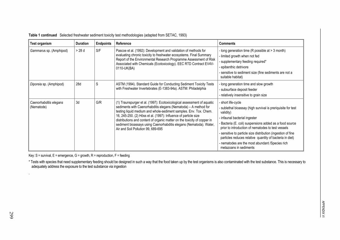
APPENDIX VI
299
Table 1 continued Selected freshwater sediment toxicity test methodologies (adapted from SETAC, 1993)
Test organism Duration Endpoints Reference Comments
Gammarus sp. (Amphipod) > 28 d S/F Pascoe et al. (1992): Development and validation of methods forevaluating chronic toxicity to freshwater ecosystems. Final SummaryReport of the Environmental Research Programme Assessment of RiskAssociated with Chemicals (Ecotoxicology). EEC RTD Contract EV4V-0110-UK(BA)
- long generation time (R possible at > 3 month)- limited growth when not fed- supplementary feeding required*- epibenthic detrivore- sensitive to sediment size (fine sediments are not asuitable habitat)
Diporeia sp. (Amphipod) 28d S ASTM (1994). Standard Guide for Conducting Sediment Toxicity Testswith Freshwater Invertebrates (E-1383-94a). ASTM: Philadelphia
- long generation time and slow growth- subsurface deposit feeder- relatively insensitive to grain size
Caenorhabditis elegans(Nematode)
3d G/R (1) Traunspurger et al. (1997): Ecotoxicological assessment of aquaticsediments with Caenorhabditis elegans (Nematoda) – A method fortesting liquid medium and whole-sediment samples. Env. Tox. Chem.16, 245-250. (2) Höss et al. (1997): Influence of particle sizedistributions and content of organic matter on the toxicity of copper insediment bioassays using Caenorhabditis elegans (Nematoda). Water,Air and Soil Pollution 99, 689-695
- short life-cycle- sublethal bioassay (high survival is preriquisite for testvalidity)
- infaunal bacterial ingester- Bacteria (E. coli) suspensions added as a food sourceprior to introduction of nematodes to test vessels
- sensitive to particle size distribution (ingestion of fineparticles reduces relative quantity of bacteria in diet)
- nematodes are the most abundant /Species richmetazoans in sediments
Key: S = survival, E = emergence, G = growth, R = reproduction, F = feeding* Tests with species that need supplementary feeding should be designed in such a way that the food taken up by the test organisms is also contaminated with the test substance. This is necessary to
adequately address the exposure to the test substance via ingestion.
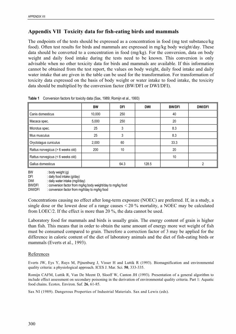
APPENDIX VII
300
Appendix VII Toxicity data for fish-eating birds and mammals
The endpoints of the tests should be expressed as a concentration in food (mg test substance/kgfood). Often test results for birds and mammals are expressed in mg/kg body weight/day. Thesedata should be converted to a concentration in food (mg/kg). For the conversion, data on bodyweight and daily food intake during the tests need to be known. This conversion is onlyadvisable when no other toxicity data for birds and mammals are available. If this informationcannot be obtained from the test report, the values on body weight, daily food intake and dailywater intake that are given in the table can be used for the transformation. For transformation oftoxicity data expressed on the basis of body weight or water intake to food intake, the toxicitydata should be multiplied by the conversion factor (BW/DFI or DWI/DFI).
Table 1 Conversion factors for toxicity data (Sax, 1989; Romijn et al., 1993)
BW DFI DWI BW/DFI DWI/DFI
Canis domesticus 10,000 250 40
Macaca spec. 5,000 250 20
Microtus spec. 25 3 8.3
Mus musculus 25 3 8.3
Oryctolagus cuniculus 2,000 60 33.3
Rattus norvegicus (> 6 weeks old) 200 10 20
Rattus norvegicus (< 6 weeks old) 10
Gallus domesticus 64.3 128.5 2
BW : body weight (g)DFI : daily food intake (g/day)DWI : daily water intake (mg/l/day)BW/DFI : conversion factor from mg/kg body weight/day to mg/kg foodDWI/DFI : conversion factor from mg/l/day to mg/kg food
Concentrations causing no effect after long-term exposure (NOEC) are preferred. If, in a study, asingle dose or the lowest dose of a range causes < 20 % mortality, a NOEC may be calculatedfrom LOEC/2. If the effect is more than 20 %, the data cannot be used.
Laboratory food for mammals and birds is usually grain. The energy content of grain is higherthan fish. This means that in order to obtain the same amount of energy more wet weight of fishmust be consumed compared to grain. Therefore a correction factor of 3 may be applied for thedifference in caloric content of the diet of laboratory animals and the diet of fish-eating birds ormammals (Everts et al., 1993).
References
Everts JW, Eys Y, Ruys M, Pijnenburg J, Visser H and Luttik R (1993). Biomagnification and environmentalquality criteria: a physiological approach. ICES J. Mar. Sci. 50, 333-335.
Romijn CAFM, Luttik R, Van De Meent D, Slooff W, Canton JH (1993). Presentation of a general algorithm toinclude effect assessment on secondary poisoning in the derivation of environmental quality criteria. Part 1: Aquaticfood chains. Ecotox. Environ. Saf. 26, 61-85.
Sax NI (1989). Dangerous Properties of Industrial Materials. Sax and Lewis (eds).

APPENDIX VIII
301
Appendix VIII Environmental risk assessment for metals and metalcompounds
Introduction
This document gives a general outline on how to perform risk assessments for metals using themethods that are available for risk assessment of new and existing organic chemicals as a startingpoint. There are a number of fundamental differences between metals and organic chemicals thatmust be taken into account when assessing the risks to man and the environment, e.g.:
• unlike most organic chemicals, metals, and a limited number of organometallo compoundslike methylmercury and methyltin, are a class of chemicals of natural origin. Consequentlynatural background concentrations and the exposure due to these background concentrationsshould be taken into account during risk assessment;
• the availability of metals for uptake by organisms under field conditions is limited, will varyfrom site to site and is highly dependent on the speciation of the metal. Hence, it is of utmostimportance that both PEC and PNEC are based on similar levels of availability in bothexposure and effect assessment, taking the speciation into account;
• the same toxic form can originate from a variety of different substances, e.g. Zn2+ fromZnSO4, ZnCl2 etc. Therefore it is in general necessary to take into account all metal speciesthat are emitted to the environment which in the end lead to concentrations of the toxicform.
Substantial levels of information are available regarding the fate and toxicity of metal ionsand this information will be examined to improve the assessment process. However, it isrecognised that many of the specific fate and toxicity extrapolations are either not appropriateor need modification. The interaction of metal ions with the media in both the aquatic andsoil compartments may result in a high level of uncertainty regarding the true level ofbioavailablity of the toxic species necessary for a practical assessment.
Organo-metallic compounds are not explicitly covered by this procedure unless they act, throughtheir degradation products, as significant sources of the toxic metal ion. It is considered that theseorgano-metallic compounds can generally be assessed as individual substances in accordance withthe procedures laid down in the main text (Chapter 3). When the emissions of these substances aremajor contributors to the toxic metal ion concentration in either a local or regional environment,they will be further assessed according to the procedures laid down in this document.
When describing the topics that need to be taken into consideration for the risk assessment ofmetals, there is often a misunderstanding with regard to definitions of some of the key terms. Inthis appendix the following definitions will be used for these key terms:
General
• total concentration of a metal: for terrestrial systems, the concentration of a metal that isdetermined after complete destruction of the mineral matrix. For aqueous systems: the totalamount of metal present, including the fraction sorbed to particles and to dissolved organicmatter and the fraction in the mineral matrix;
• available fraction: the fraction of the metal that is extractable from the substrate withchemical (e.g.: neutral salt, water extraction) or physical means (shaking, pore water

APPENDIX VIII
302
collection), and that is generally considered to be a better estimate for the fraction that ispotentially available for organisms than the total concentration;
• bioavailable fraction: the fraction that is available for uptake by a specific organism. Asingle substrate has only one 'availability' for each of the possible physico-chemicalextraction procedures. The bioavailability differs, however, per biological species. Thus,taking soil as an example, for instance for worms in a certain soil the bioavailability may behigh (it is in this case the concentration in the pore water that determines uptake), while forarthropods in the same soil the bioavailability may be low (uptake by the food is for theseorganisms the dominant uptake route);
• natural background concentration: the concentration that is present due to natural causesonly;
• ambient background concentration: the concentration that is present due to naturalbackground plus the immission of metals from diffuse sources of human origin9.
For soils or sediments
• water extractable fraction or concentration: the fraction or the concentration of the metalthat is extracted after shaking the substrate in aqueous solution (usually distilled water);
• neutral-salt solution extractable fraction or concentration: the fraction or theconcentration of the metal that is extracted after shaking the substrate in neutral saltsolution;
• pore water concentration: the concentration of the metal that is present in the pore watercollected from the substrate;
• pore water activity: the concentration of a metal in the aqueous fraction that is potentiallybiologically active (usually considered to be the concentration of metal ions that can betaken up by organisms).
Exposure assessment
For the assessment of metals it is in general necessary to take into account all metal species thatare emitted to the environment which in the end lead to concentrations of the bioavailablespecies that may cause effects. In practice, a limited number of major emissions or usespredominate and these must initially be identified. The assessment will normally concentrate onthe impact of these emissions since they will be the major contributors to the regional burden,but due care must be paid to the impact of local emissions of specific substances. An inventoryof all relevant emission sources must be prepared and specific industry and use categoriesidentified for assessment of both local and regional impact.
Two types of emission can be identified: diffuse emissions and point source emissions. For somemetal compounds, diffuse sources such as emissions from agriculture, transport, corrosion etc
9 In case of soil, for all metals so-called reference lines were derived by correlating measured ambient background
concentrations (total concen-trations in the soil-matrix) at a series of remote rural sites in the Netherlands to thepercentage lutum (%L) and the organic matter content (%H) of these soils (Ministry of VROM, 1994). The sameapproach has been followed in Flanders, Belgium (Ontwerp uitvoeringsbesluit, 1995). To this end the 90-percentiles of the ambient background concentrations measured were used. The metal-specific parameters of theregression equations represent the strength of binding of the different metals to soils of different clay and humuscontents. The reference lines are not only used to calculate ambient background concentrations at given sites, butalso to enable the extrapolation of laboratory toxicity data to standard-soil conditions.Some typical examples of reference lines derived in The Netherlands ([ ] = ambient background concentration inmg/kg soil, L = % lutum, H = % organic matter): [Cu] = 15 + 0.6 . (L + H) ; [Zn] = 50 + 1.5 . (2L + H) or [Ni] = 10+ L.

APPENDIX VIII
303
can make a significant contribution to the overall levels. For many substances, however, localemissions from point sources will need to be considered as well as the wider contribution to theregional burden. New substances, for example, must be assessed for their impact following localemissions. In general their contribution to the larger environmental burden will be small untilhigh annual tonnages are reached.
Local exposure assessment
As with organic compounds, the precise emissions will need to be identified and quantified forthe whole life-cycle of the substance. Emission factors should initially be based on the substancebeing considered. It is important to know whether the substance is soluble in water, or can betransformed into a soluble form. Thus some knowledge of the chemistry of the particularsubstance and its interaction with the receiving media is important. Where the metal compoundis soluble or can be transformed to a soluble form, the prediction of the environmentalconcentration, PEClocal, can be based on the relevant soluble metal ion. The behaviour of thesubstance in a wastewater treatment plant can be modelled using SimpleTreat, althoughmeasured Kp values will have to be used (Section 2.3.7 of main text). Since the actualbioavailability of the metal ion will be determined by the properties of the receiving media, suchas the pH and water hardness, the precise physico-chemical characteristics of this receivingmedia must be defined. In general, it will be defined in a way which optimises the bioavailabilityof the toxic species. Speciation models exist which may be used to determine the solublefraction. The partitioning behaviour of the substance to sludge/sediment/soil can be based on theappropriate Kp values for the soluble ion.
In some cases, the metal compound will be only poorly soluble and sufficiently stable to notrapidly transform to a water soluble form. In these circumstances, the substance itself should beassessed taking into account its specific partitioning characteristics. For the aquatic environment,it can be assumed as a first estimate that the substance will dissolve up to its water solubilitylimit, and that this fraction will be the bioavailable form. Refinement of the assessment may takeinto account kinetics of the dissolution.
Regional exposure assessment
As for organic substances, all emissions from both point and diffuse sources are assumed tocontribute to the regional concentration, PECregional. Because of the wide range oftransformation processes and longer timescales involved, it is assumed that all the individualmetal compounds are changed to the ionic species. Where possible, information on kinetics oftransformation processes should be taken into account.
As bioavailability is influenced by various physico-chemical characteristics of the environment itis important to define a 'standard environment', especially for a regional assessment. It isproposed that a regional assessment is carried out under conditions that optimise the bioavailabilitywith respect to ranges for pH, water hardness etc that are found in the natural environment. Thisenvironment will probably differ for each metal assessed. Multimedia fate models can be used toassess exposure of man and ecosystems to metals on a regional scale. In applying multimedia fatemodels all emissions, including point sources, are assumed to be diffuse.
Transport of metals between the aqueous phase and soil/sediment/suspended matter should bedescribed on the basis of measured soil/water, sediment/water and suspended matter/waterequilibrium partition coefficients (Kp), instead of using common mathematical relationshipsbased on, for example, octanol-water partition coefficients, as is usually done for organic

APPENDIX VIII
304
chemicals (see Section 2.3.4 of the main text). The same applies to the bioconcentration factorsrequired: only experimentally determined values should be used (see Section 3.8 of the main textand Section 3.3 of this appendix). For soils, the Kp values to be used should, as far as possible,be derived for the soil type of interest. The soil usage should also be taken into account (forinstance cultivated versus non-cultivated soils) since this may be of importance for the mostappropriate Kp values. Often volatilisation is to be ignored. In such cases, most of the metalpresent in the atmosphere is predominantly bound to aerosols which means that rates of dry andwet deposition (in combination with the scavenging ratio) of atmospheric aerosols will suffice toquantify transport from the atmosphere. If biotransformation occurs this must be taken intoaccount.
More specific guidance on the use of regional fate models is given in Figure 1.
In general, the mathematical descriptions of fate processes used in multimedia fate models arealso applicable to local models.
Background concentrations
When assessing the exposure of man and ecosystems to metals previous releases into theenvironment need to be considered. In view of differences in bioavailability (see below) it isimportant to distinguish between ambient background concentrations and natural backgroundconcentrations. One should be aware that natural background concentrations within anenvironmental compartment may vary from site to site by several orders of magnitude. Also, dueto natural dynamic processes like weathering, natural background concentrations may changeover time. This means that it is impossible to attribute single values to natural backgroundconcentrations of specific metals within a certain compartment. It should be noted that undernatural conditions in certain regions, clearly elevated natural background concentrations can beencountered. When assessing the natural background concentration within a certain area, these“outliers” should not be used or included in the calculation of the standard backgroundconcentrations as they would give a non-representative picture thereof.
Several methods are available for determining background concentrations. Apart from theobvious method of measuring metal levels at selected sites considered to be undisturbed byhuman activities, additional methods include:
Geochemical modelling: estimation methods on the basis of the contribution of weatheringprocesses (erosion). This method is shown to be well applicable for assessing naturalbackground concentration in aqueous systems (rivers).
Assessment of metal concentrations in the deeper sediment layers, taking into accountanthropogenic contributions and leaching to these layers.
For surface water having ground water as its origin: assessment of the metal concentrations inthe deeper ground water.
For soils, ambient background concentrations can be calculated as described above (referencelines). Through this procedure the natural binding capacity of soils, making the metal more orless inert in the solid phase, is approximated. Application of this procedure to both laboratorytoxicity data and to field soils is possible.
For surface water extensive national monitoring programs exist for the follow-up of metals in theaquatic environment since most metals are considered in the EC Regulation 76/464 as list I(“black list”) or list II (“grey list”) substances. Extraction of representative natural background

APPENDIX VIII
305
concentrations may be possible from these data. However, these monitoring programs oftenmeasure total instead of dissolved metal concentrations.
Equilibrium partitioning/bioavailability
One should be aware that Kp values are both environment (site) and compound specific, anddepend on the speciation of the metal in both the solid and the liquid (pore water) phase. Thespeciation of metals is strongly influenced by environmental factors like for instancetemperature, redox conditions, pH, and composition of both the liquid and solid phase.

APPENDIX VIII
306
Multimedia fate models can be used to estimate exposure to metals. However, there are severaldifferences compared to the use of these models for organic compounds. Below, differences aredescribed for applying regional models. Reference is made to the sections in the main text.
1. Physico-chemical properties (section 2.3.2)In general water solubility, boiling point and vapour pressure cannot be used. The octanol-waterpartitioning coefficient is not appropriate and measured partition coefficients Kp should be usedinstead.
2. Partition coefficients (section 2.3.5)Adsorption to aerosol particlesMost of the metal present in the atmosphere will be bound to aerosols. Therefore, an extremelylow value for the vapour pressure should be used in formula 5 on page 31, e.g. 10-20 Pa. Thisleads to a value for Fassaer almost equal to one. If a valid measured value is available, this valuecan be used.
VolatilisationVolatilisation can be ignored for metals, except for mercury-compounds and severalorganometallo compounds. Therefore the Henry-coefficient should be set to a very low value(formula 6).
Adsorption/desorptionFormula 8 and 9 cannot be used. As stated in this appendix, measured Kp values must be usedfor water-soil, water-sediment and water-suspended matter.
3. Biotic and abiotic degradation rates (Section 2.3.6)Not important for regional models.
4. Elimation processes prior to the release in the environment (Section 2.3.7)For applying models like SimpleTreat a partition coefficient is used for water-sludge. Formetals a measured Kp value must be used. However, it should be noted that Kp values aredifferent for the different metal species.
5. Calculation of PECregional (Section 2.3.8.7)The values applied for model parameters for the regional model (Table 10), intermedia masstransfer coefficients (Table 11) and model parameters for the continental concentration (Table12) can be used.
Figure 1: Use of multimedia fate models for metals
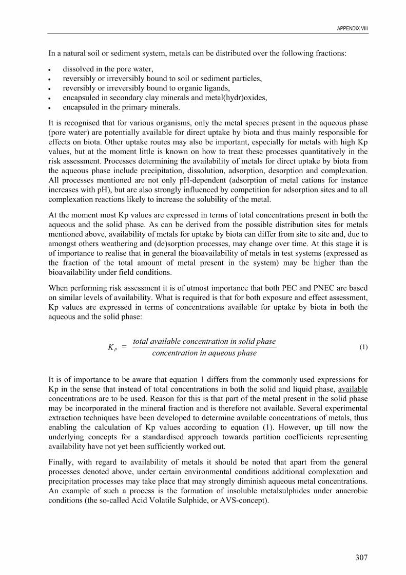
APPENDIX VIII
307
In a natural soil or sediment system, metals can be distributed over the following fractions:
• dissolved in the pore water,• reversibly or irreversibly bound to soil or sediment particles,• reversibly or irreversibly bound to organic ligands,• encapsuled in secondary clay minerals and metal(hydr)oxides,• encapsuled in the primary minerals.
It is recognised that for various organisms, only the metal species present in the aqueous phase(pore water) are potentially available for direct uptake by biota and thus mainly responsible foreffects on biota. Other uptake routes may also be important, especially for metals with high Kpvalues, but at the moment little is known on how to treat these processes quantitatively in therisk assessment. Processes determining the availability of metals for direct uptake by biota fromthe aqueous phase include precipitation, dissolution, adsorption, desorption and complexation.All processes mentioned are not only pH-dependent (adsorption of metal cations for instanceincreases with pH), but are also strongly influenced by competition for adsorption sites and to allcomplexation reactions likely to increase the solubility of the metal.
At the moment most Kp values are expressed in terms of total concentrations present in both theaqueous and the solid phase. As can be derived from the possible distribution sites for metalsmentioned above, availability of metals for uptake by biota can differ from site to site and, due toamongst others weathering and (de)sorption processes, may change over time. At this stage it isof importance to realise that in general the bioavailability of metals in test systems (expressed asthe fraction of the total amount of metal present in the system) may be higher than thebioavailability under field conditions.
When performing risk assessment it is of utmost importance that both PEC and PNEC are basedon similar levels of availability. What is required is that for both exposure and effect assessment,Kp values are expressed in terms of concentrations available for uptake by biota in both theaqueous and the solid phase:
pK = total available concentration in solid phaseconcentration in aqueous phase
(1)
It is of importance to be aware that equation 1 differs from the commonly used expressions forKp in the sense that instead of total concentrations in both the solid and liquid phase, availableconcentrations are to be used. Reason for this is that part of the metal present in the solid phasemay be incorporated in the mineral fraction and is therefore not available. Several experimentalextraction techniques have been developed to determine available concentrations of metals, thusenabling the calculation of Kp values according to equation (1). However, up till now theunderlying concepts for a standardised approach towards partition coefficients representingavailability have not yet been sufficiently worked out.
Finally, with regard to availability of metals it should be noted that apart from the generalprocesses denoted above, under certain environmental conditions additional complexation andprecipitation processes may take place that may strongly diminish aqueous metal concentrations.An example of such a process is the formation of insoluble metalsulphides under anaerobicconditions (the so-called Acid Volatile Sulphide, or AVS-concept).
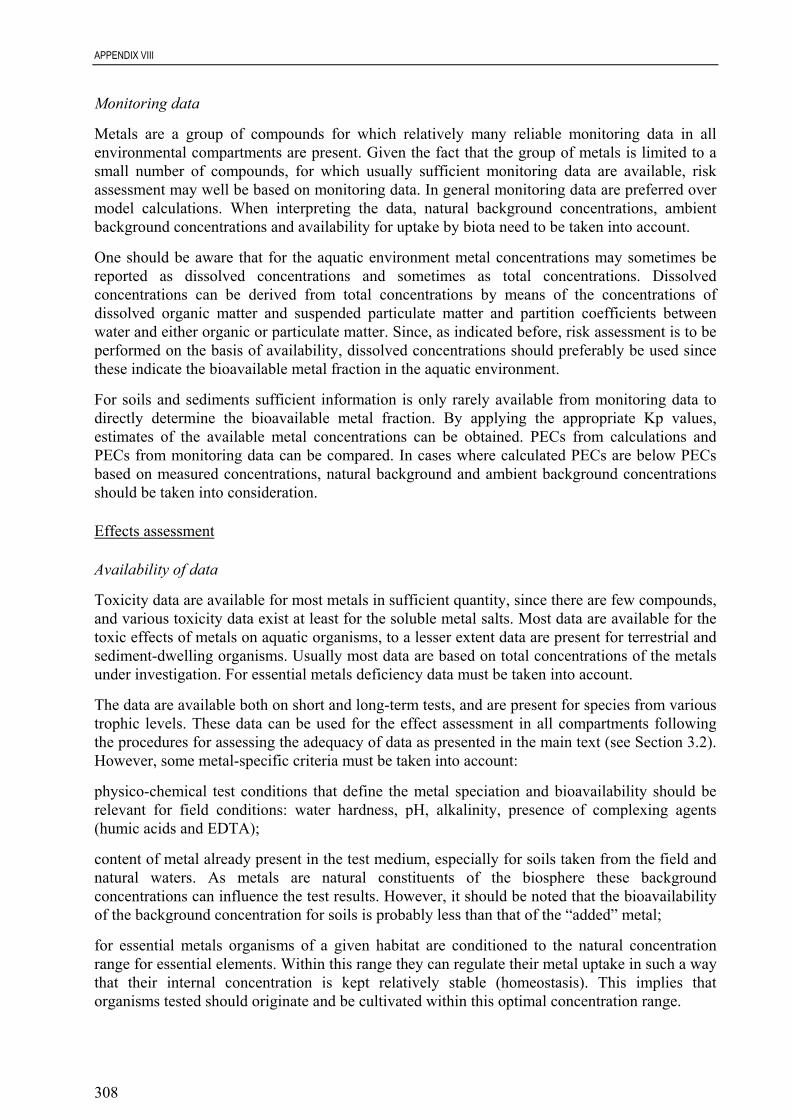
APPENDIX VIII
308
Monitoring data
Metals are a group of compounds for which relatively many reliable monitoring data in allenvironmental compartments are present. Given the fact that the group of metals is limited to asmall number of compounds, for which usually sufficient monitoring data are available, riskassessment may well be based on monitoring data. In general monitoring data are preferred overmodel calculations. When interpreting the data, natural background concentrations, ambientbackground concentrations and availability for uptake by biota need to be taken into account.
One should be aware that for the aquatic environment metal concentrations may sometimes bereported as dissolved concentrations and sometimes as total concentrations. Dissolvedconcentrations can be derived from total concentrations by means of the concentrations ofdissolved organic matter and suspended particulate matter and partition coefficients betweenwater and either organic or particulate matter. Since, as indicated before, risk assessment is to beperformed on the basis of availability, dissolved concentrations should preferably be used sincethese indicate the bioavailable metal fraction in the aquatic environment.
For soils and sediments sufficient information is only rarely available from monitoring data todirectly determine the bioavailable metal fraction. By applying the appropriate Kp values,estimates of the available metal concentrations can be obtained. PECs from calculations andPECs from monitoring data can be compared. In cases where calculated PECs are below PECsbased on measured concentrations, natural background and ambient background concentrationsshould be taken into consideration.
Effects assessment
Availability of data
Toxicity data are available for most metals in sufficient quantity, since there are few compounds,and various toxicity data exist at least for the soluble metal salts. Most data are available for thetoxic effects of metals on aquatic organisms, to a lesser extent data are present for terrestrial andsediment-dwelling organisms. Usually most data are based on total concentrations of the metalsunder investigation. For essential metals deficiency data must be taken into account.
The data are available both on short and long-term tests, and are present for species from varioustrophic levels. These data can be used for the effect assessment in all compartments followingthe procedures for assessing the adequacy of data as presented in the main text (see Section 3.2).However, some metal-specific criteria must be taken into account:
physico-chemical test conditions that define the metal speciation and bioavailability should berelevant for field conditions: water hardness, pH, alkalinity, presence of complexing agents(humic acids and EDTA);
content of metal already present in the test medium, especially for soils taken from the field andnatural waters. As metals are natural constituents of the biosphere these backgroundconcentrations can influence the test results. However, it should be noted that the bioavailabilityof the background concentration for soils is probably less than that of the “added” metal;
for essential metals organisms of a given habitat are conditioned to the natural concentrationrange for essential elements. Within this range they can regulate their metal uptake in such a waythat their internal concentration is kept relatively stable (homeostasis). This implies thatorganisms tested should originate and be cultivated within this optimal concentration range.

APPENDIX VIII
309
Derivation of the PNEC
PNECs can be derived through the application of assessment factors on the basis of the availabledata assessed according to the criteria given above. Standard methods applied elsewhere (e.g. fororganic compounds) can be used for this (see Sections 3.3/3.7 of the main text). However,because of the specific mode of action that metals may have for some species, care should betaken in extrapolating short-term toxicity data to the PNEC using the standard assessment factorsin Section 3.3. For many metals sufficient long-term toxicity data for aquatic organisms may bepresent to enable statistical extrapolation, results of which can support the results of PNECscalculated using assessment factors.
Calculated PNECs derived for essential metals may not be lower than natural backgroundconcentrations.
A prerequisite for the derivation of the PNEC is that it is done on the basis of the same level ofavailability as in exposure assessment:
Results from aquatic toxicity tests are usually expressed as total concentrations. As a firstapproach total concentrations have to be recalculated to dissolved concentrations using partitioncoefficients. If this is not possible, the total concentration can be set equal to the dissolvedconcentration. Differences in test systems, e.g. (semi-)static versus continuous flow systems andnatural versus standard water, have to be considered;
For the terrestrial compartment many data exist, but most are only expressed as totalconcentration that has been added to the test media. This added amount will be partitionedamong the aqueous and the solid phase. Application of partition coefficients to calculate theavailable concentration in soil can be applied. Soil type correction, using reference lines shouldbe applied to correct for differences among soil types (see also Section 3.6.2 of the main text).
In future risk assessment for the terrestrial compartment one should be aware of the differentroutes of exposure that exist among terrestrial species: for species that are not exposed throughthe aqueous phase, the (physico-chemically) available fraction needs not be correlated to thebioavailability;
Some of the metals are essential metals, having a function in biological processes at lowconcentrations. Shortage of micronutrients may cause malfunction. This implies that in settingthe PNEC information on deficiency levels should be taken into account. It should, however, benoted that often no information on deficiency levels of various metals for various species isavailable.
Though some exceptions exist, in general ionic metal species are considered to be the dominantmetal species taken up, and are thus considered to be the metal species responsible for the toxiceffect. Data on the concentration of ionic species in aquatic and terrestrial systems are notreadily available, and cannot, as yet, be applied on a regular basis in risk assessment.
Bioaccumulation of essential metals
Metals are taken up by organisms. For essential metals, biota regulate their uptake by means ofthe general physiological mechanism of homeostasis. By this mechanism, organisms will keepwithin a certain range of varying external concentrations, their intracellular levels relativelyconstant, in order to satisfy their requirements for that essential element. Homeostasis impliesthat organisms can deliberately concentrate essential elements if concentrations in theenvironment are very low. This may lead to high BCF values. On the other hand, the
APPENDIX VIII
310
homeostatic regulation capacity will be exceeded at a given higher external concentrationbeyond which the element will accumulate and become toxic.
Risk Characterisation
The risk characterisation of metals basically follows the principles set out in Section 4 of themain text. However, it should be stated again that is very important that both PEC and PNEC arebased on similar levels of availability. In addition, when PEC/PNEC ratios greater than one arefound, it is very important to have information on the natural and/or ambient background levelsin order to decide upon further actions to be taken to reduce the risks.
Since for most metals sufficient monitoring data are obtainable, risk assessment will often bebased on measured instead of calculated environmental concentrations, especially for a regionalassessment. Usually most monitoring data deal with total concentrations. Especially in case ofaqueous systems it often is well possible to convert measured total concentrations to dissolvedconcentrations. For terrestrial systems this is possible by applying the appropriate Kp values.
References
Cleven RFMJ, Janus JA, Annema JA and Slooff W (eds.) (1993). Integrated Criteria Document Zinc. RIVM reportNo. 710401028.
Luoma SN (1983). Bioavailability of trace metals to aquatic organisms - a review. The Science of the TotalEnvironment 28, 1-22.
Ministry of VROM (1994). Environmental Quality Objectives in the Netherlands, Den Haag, The Netherlands.
Ontwerp-uitvoeringsbesluit bij het vlaamse bodemsaneringsdecreet (24-01-1995) houdende achtergrondwaarden enbodemsaneringsnormen (document on background concentrations in Flanders, Belgium).
Parametrix Inc. (draft February 1995). Aquatic Ecotoxicity Testing of Sparingly Soluble Metals and MetalCompounds. Prepared for the Mining Association of Canada, Washington.
Ure AM, Davidson CM (eds.) (1995). Chemical Speciation in the Environment. Blackie Academic & Professional,Glasgow.
Van der Kooij LA, van de Meent D, van Leeuwen CJ, Bruggeman WA (1991). Deriving quality criteria for waterand sediment from the results of aquatic toxicity test and product standards: application of the equilibriumpartitioning method. Wat. Res. 25, 697-705.
Van Tilborg WJM and van Assche F (1995). Integrated Criteria Document Zinc: Industry Addendum. ProjectgroepZink BMRO-VNO, Roozendaal.
Van Wensem J, Vegter JJ, van Straalen NM (1994). Soil quality derived from critical body concentrations of metalsin soil invertebrates. Appl. Soil Ecol. 1, 185-191.
Wood JM (1974). Biological cycles for toxic elements in the environment. Science 188, 1049-1052.
APPENDIX IX
311
Appendix IX Environmental risk assessment for petroleum substances
Introduction
In the present appendix the Hydrocarbon Block Method (HBM) is described, which is underdevelopment and may be used for environmental risk assessment of petroleum substances. Themethod was originally devised by CONCAWE (The Oil Companies' European Organisation forEnvironmental and Health Protection) and was discussed in a workshop in Ispra in December1994 (CONCAWE, 1995; EU, 1995). The approach has only recently been devised and henceexperience with its application is limited. Although there has been work to validate the generalapproach, it should be recognised that there are still uncertainties regarding some technicaldetails which should be borne in mind, when considering the outcome of the riskcharacterisation.
Outline of the method
There are many petroleum substances (e.g. refinery streams and solvents) which althoughdescribed by a single EINECS number are hydrocarbon mixtures of varying degrees ofcomplexity. The compositional complexity of many petroleum hydrocarbon substances iscompounded by the fact that their composition will vary depending on the source of crude oiland the details of the process used in their production. This compositional complexity posesparticular problems when environmental risk assessment is required.
Difficulties in carrying out a risk assessment for petroleum substances arise because individualcomponents of them have specific and different physico-chemical and ecotoxicologicalproperties, and potentials to be degraded in the environment. Each will be subjected to differentdistribution and fate processes on release. This means that on release to the environment, eachcomponent will behave independently and reach its own concentration in each environmentalcompartment. It follows from this, that a PEC for the whole petroleum substance does not exist.It would in theory, be possible to identify each individual component of a petroleum substanceand then to determine a PEC for each of them. In practice this approach demands a degree ofanalytical resolution that is not achievable for most petroleum substances and even wherepossible, handling such large quantities of data would be impractical. However, sincehydrocarbons of similar structure will have similar physico-chemical properties and potentials tobe degraded in the environment they will have similar distributions and fates within a givenenvironment. It is therefore possible to group or “block” such hydrocarbons, so that componentshaving similar properties may be considered together (it should be recognised that a “block” mayconsist of a single component or a large number of components with similar fate and distributionproperties). Once the “blocks” for a substance have been established, PEC values can becalculated for each “block” for each environmental compartment. Given that PECs can only beobtained for single components , or groups of similar components, it follows that PNECs mustalso be estimated for the same individual components or groups of components.
Therefore, ecotoxicity data obtained on the whole substance, whether obtained using wateraccommodated fractions (WAFs) or dispersions, cannot be used to estimate PNECs. PNECsmust be based on the toxicity of the individual “blocks”, be they single or multiple component“blocks”. These blocks should show similar modes of action.
From the above it is clear that the PEC/PNEC ratio of the whole substance cannot be deriveddirectly, as neither the PEC, nor the PNEC for the whole substance will be available. ThePEC/PNEC ratio is therefore derived from the PEC/PNEC ratios of the “blocks” of components,

APPENDIX IX
312
based on the proportional contribution of each of the “blocks” to the composition of the wholesubstance, and assuming that effects will be concentration additive:
PECPNEC
whole substance = PECPNEC
+ PECPNEC
+ PECPNEC
etc.A
A
B
B
C
C(2)
where:A,B,C etc. are the “blocks”.
This is referred to as the Hydrocarbon Block Method (HBM).
In relation to the above it should be noted that where the petroleum substance is of such limitedcomplexity that it can be considered to constitute a single “blocks” (e.g. some narrow-cuthydrocarbon solvents) then the risk assessment is identical to that for a simple single componentsubstance i.e. the substance is a single “blocks” and therefore, the PEC for the petroleumsubstance and the “blocks” are the same, the ecotoxicity data used to obtain the PNEC can bebased on the toxicity of the whole substance, and the PEC/PNEC ratio can be obtained directly.
Given the complexity of many of the petroleum substances and hence the number of “blocks”that will be created, allied with the need for flexibility in the assessment procedures, it isconsidered that the use of this method of risk assessment for petroleum substances will, inpractice, only be possible using computer based assessment procedures.
In view of the fact that particular “blocks” of hydrocarbons may be present in more then onepetroleum substance, there may be a need to consider the contribution to the overallenvironmental risk from more then one petroleum substance. In principle the HBM allows forcalculating the combined environmental risks of different petroleum substances in specificsituations or for the comparison of combined PEC values with monitoring data. For this, thePEC/PNECs of the different discharged petroleum substances (or the values for their specificblocks) can be combined in the same way as the blocks for a specific petroleum substance arecombined, assuming that the effects will be concentration additive.
Outline of the application of the hydrocarbon block method
The following outlines the principal steps in the application of the HBM:
• obtain compositional data for the substance that are sufficient to assign components to“blocks”;
• define “blocks” by grouping components on the basis of similar structural and/or physico-chemical properties, degradation parameters and ecotoxicological properties. If desired,“blocks”can be defined as single components;
• obtain production and use data;• establish release estimates for each “blocks”. A single release estimate for a petroleum
substance may not always be adequate: “blocks” with markedly different physico-chemicalproperties may require different release estimates;
• assign representative values for physico-chemical properties, degradation rate constants andLC/EC50s and NOECs for each “blocks”;
• determine the PEC value for each compartment for each “blocks” (local as well as regional);• determine the PNEC value for each “blocks”• calculate PEC/PNEC ratio for each “blocks”and sum proportionally.
APPENDIX IX
313
Summarising, once the “blocks” with their physico-chemical and ecotoxicological properties aredefined, there is no difference between the approach presented in the main text of the TechnicalGuidance Document and the HBM. This means that a PEClocal and PECregional can becalculated as described in Chapter 2 of the main text and a PNEC can be derived as described inChapter 3 of the main text.
Points for special consideration when using the HBM for risk assessment
The more detailed description of certain aspects of the application of the HBM which follows, islargely based on the application of the HBM to risk assessment for the aquatic environment. Thisis because it is considered that given the present state of the development of environmental riskassessment, and of the use of the HBM in particular, the use of this compartment bestexemplifies the principles, applicability and the issues associated with the use and furtherdevelopment of the HBM.
Composition of petroleum substances
The composition of many petroleum substances is complex, with a single substance oftencontaining a large number of component chemicals, varying in chemical type, molecular weightand isomeric structure.
For some petroleum substances the differences in the physico-chemical properties of thedifferent “blocks” will be such that a single release estimate for the substance may not besufficient and separate release estimates for some “blocks” or groups of “blocks” may berequired.
The complexity of some petroleum substances is further compounded by the fact that theircomposition may vary depending on the source of the crude oil from which they are producedand the method of their production. It is therefore necessary, that adequate information beavailable not only on composition but also, where relevant, on variations in composition. Thisinformation can be used to allow several calculations of the PEC/PNEC for a substance to takeaccount of likely variations in composition. For petroleum substances, adequate information oncomposition may allow risk assessment of groups of substances to be undertaken at the sametime, for example whole groups of naphthas or kerosines.
It is clear that for many petroleum substances a complete resolution of the composition is neitherachievable nor necessary to be able to carry out a risk assessment. But it is essential thatcompositional data, including information on variability, is sufficient to allow “blocks” to beproperly defined for the purpose of risk assessment.
It should be borne in mind that some petroleum substances will contain a relatively narrow rangeof components and be much more consistent in composition e.g. some narrow-cut hydrocarbonsolvents. In some cases it may be appropriate to regard such substances as a single “block”.
Many of the components of petroleum substances will be present in many of the substances. Ingeneral it is desirable to ensure, that when similar components are present in different petroleumsubstances the same approach to “blocking” is taken. This will allow the development ofPEC/PNEC ratios for “blocks” applicable to a range of petroleum substances (data on physico-chemical and degradation properties and toxicity values for these “common blocks” will onlyneed to be generated once).
APPENDIX IX
314
Definition of “blocks”
“Blocks” will primarily be defined on the basis of those physico-chemical and degradationproperties that are key in determining the distribution and fate of their components. Care shouldbe taken to ensure that “blocks” are not so wide as to encompass components that will not havebroadly similar fates and distributions on release. Similarly, “blocks” should, whenever possible,contain substances with a similar mode of action and a narrow range of toxicity. Both the fateand toxicity criteria for “blocks” definition need to be satisfied simultaneously.
Verburgh et al. (1995) carried out “trial calculations” using the HBM based on data for 500hydrocarbons with a non-specific mode of action, using non-polar narcotic toxicity QSARs andwith the Mackay level III model of the EU standard environment defined for calculating thePECregional. It appeared that for definition of the “blocks” the log Kow is the main parameter.This implies that “blocks” can be defined on equally spaced log Kow values: e.g. <3.0; 3-3.5;3.5-4.0 etc.
It is proposed to start with such a “block definition” for application of the HBM. Based on theresults of the risk assessment the “blocks” may be further refined.
“Blocks” based on, or containing, non-hydrocarbons
Certain petroleum substances contain non-hydrocarbon components. Special care should betaken when assessing these substances to ensure that “blocking” is appropriate and in particularthat the range of toxicities of components in the “block” is small and that where necessary, dueaccount is taken of differences in mode of action.
Additivity of toxicity
It is generally accepted that for chemicals with the same mode of action, acute toxicities can beconsidered as additive (EIFAC, 1987). There is increasing evidence that this is also true forchronic toxicity (Hermens, 1989).
Whether a chemical or a group of related chemicals act by non-polar narcosis can be based on acomparison of test results with QSAR estimates for base-line toxicity. Schemes exist that allowthe classification of large numbers of organic chemicals according to their mode of action(Verhaar et al., 1992).
Petroleum hydrocarbons are for the great part composed of hydrocarbons. These act via a similarmode of toxic action, non-polar narcosis. In the light of the above it can be assumed that for thehydrocarbon components of petroleum substances, effects will be simple concentration additive.
The situation is less clear with regard to chemicals with different modes of action. Componentsof petroleum hydrocarbons with specific modes of action are likely to be “blocked” together,provided they have the same specific mode of action. In the first instance the PEC/PNEC ratio ofthis “block” shall be added to the total PEC/PNEC ratio. From this it will be clear if thePEC/PNEC ratio for that “block” influences any potential for environmental risk for the specificpetroleum substance. If it does, further investigation whether or not there is additivity of themodes of action, would be required.
Chemicals which may have a specific mode of action present in petroleum substances can bemetallic constituents (e.g. vanadium and nickel in crude oil, fuel oils and asphalt) andheterocyclic compounds (e.g. carbazole compounds in cracked fuels) and mutagens/ carcinogens(e.g. PAHs such as benzo(a)pyrene, 7,12-dimethylbenzo(a)anthracene. However, they are

APPENDIX IX
315
present in low concentrations compared to the non-specific acting components. Nevertheless,these specific acting constituents should on a case-by-case basis be taken into account in theenvironmental risk assessment at least in a qualitative way.
QSARs
The identification of the blocks when applying the HBM may be dependent on the use of QSARsfor the estimation of physico-chemical properties (e.g. log Kow, water solubility, melting pointand vapour pressure) and degradation rates (e.g. photodegradation and hydrolysis rates), whenmeasured values are not available. There are reasonably well accepted methods for thegeneration of these data using readily available data bases, or QSARs. There are no widelyaccepted QSARs for biodegradation, but it is considered adequate, at least for screening, ifexperimentally determined rate constants for the “blocks” of interest are not available, to useQSAR estimates for block identification, according the principles laid down in Chapter 4 on theUse of QSARs.
The use of QSARs is well established for predicting the acute toxicity of simple hydrocarbons,and can be used to supplement the available ecotoxicity data. Whilst the accuracy of QSARs formore complex hydrocarbons and for chronic toxicity may need further consideration, theyprovide an adequate default where experimental data are not available (in particular where thevalues are found not to be key to the outcome of the risk assessment).
The minimum data-set available for each priority petroleum substances, is usually not sufficientfor risk assessment using the HBM, because it will usually comprise tests conducted with thewhole petroleum substance. Since in the HBM process individual hydrocarbons are blockedtogether on the basis of their environmental fate and ecotoxicological properties, additional dataon these hydrocarbons are also required. These may be measured data, but it is foreseen thatvalues derived from QSARs will be helpful for filling datagaps in the establishment of blocks.When the overall risk assessment for the petroleum substance is undertaken (with thePEC/PNEC ratios for the blocks calculated and summed), those blocks contributing most to theoverall PEC/PNEC ratio can be identified. It should be noted that any decision on the finaloutcome of the risk assessment when the overall PEC/PNEC ratio is close to or greater than one,will need to be based on measured (rather than QSAR) data. Hence, for each block (unless thecontribution of the particular block is found to be irrelevant to the outcome of the riskassessment), representative measured base-set data should be available. These data could be onany component of the block, since by definition, blocks are comprised of hydrocarbons withsimilar fate and ecotoxicological properties. Data on some individual hydrocarbons suitable forthis purpose, are already available as the IUCLID database shows.
For “block” identification, QSARs for short (algae, daphnids and fish) and long-term (daphnidsand fish) toxicity are given in Chapter 4 on the use of QSARs. These QSARs can be used forchemicals with a non-specific mode of action, i.e. for most petroleum substance components.Considering the assessment factors presented in the TGD (see Section 3.3.1 of the main text) afactor of 10 on the QSAR derived long-term NOEC is proposed. More guidance on the use ofQSARs in general can be found in Chapter 4.
“Blocks” which do not exhibit acute toxicity
There will be a number of “blocks” for which no acute toxicity is indicated at the limit of watersolubility. Adema (1986, 1991) found no short-term toxicity for n-decane or higher homologuesand for alkylbenzenes with a carbon number higher than 14. This does not necessarily mean that

APPENDIX IX
316
these “blocks” will not contribute to chronic toxic effects. There may be several approaches toestimate chronic toxicity for such chemicals if there are no measured long-term toxicity dataavailable:
• use the QSAR for long-term toxicity as presented in Chapter 4 of the TGD. However, theseQSARs can only be applied in a range of log Kow from approximately 2-6. For chemicalswith higher log Kow the resulting NOEC is often higher than the water solubility.
• for blocks which do not demonstrate acute toxicity at or below their water solubility,QSARs (irrespective of the fact that the result may exceed the water solubility) may be usedas a basis for the PNEC by application of a suitable assessment factor. This calculated valueis taken to represent the PNEC of the block unless, it is itself greater than the watersolubility. In this case the water solubility should be substituted as the PNEC. It should benoted that for very high log Kow values, this may lead to unrealistic PNEC values;
• as an indication above log Kow 6, a parabolic equation to derive a BCF for fish can be used(see Section 3.8.3.2 of main text and Chapter 4) in combination with the critical bodyburden concept (McCarty & Mackay, 1982) to calculate the chronic toxicity. This criticalbody burden concept indicates that the long-term critical body burden is equal to the NOECmultiplied by the BCF (CBB = BCF.NOEC) (Sijm et al., 1992; ECETOC, 1995). To be ableto perform a risk assessment, there may be a need to develop measured chronic data tosupport this QSAR prediction.
Undissolved material
Petroleum substances (or components of them) can enter the aquatic environment either insolution or as undissolved material in slicks or dispersions. Hydrocarbons in undissolved formmight have direct local effects. It is considered that undissolved hydrocarbons will not be presentat the regional level, but in any event this will have to be confirmed by calculating thePECregional.
Monitoring data
For substances consisting of only a single component sound and relevant monitoring data may beavailable for several compartments. For petroleum substances there are a number of difficultiesrelated to the use of monitoring data that need specific consideration. Frequently there will bemeasurements of total hydrocarbons or of particular hydrocarbon components that may havecome from a range of different petroleum substances.
Such release or monitoring data may be used to provide a worst-case estimate of theconcentration of a “block” for screening purposes, assuming that the whole of the release isattributable to the particular petroleum substance. However, it should be noted that the measuredconcentrations represent the sum of all sources of a block whereas the calculated concentrationsfor a specific “block” represents only the fraction of the total concentration of this “block” in theenvironment related to the specific petroleum substance under study. Therefore, monitoring dataare most suitable for the assessment of a certain “block”, as they represent the actualconcentration the organisms are exposed to in the environment, related to all relevant sources.
Compartments other than the aquatic
The description of the use of the HBM for the environmental risk assessment of petroleumsubstances given above, has focused on the aquatic environment. This is because at the presenttime it is only for this environmental compartment that sufficient data and experience are

APPENDIX IX
317
available to allow anything approaching a full risk assessment. However, the principles of theHBM are applicable to all environmental compartments and it is anticipated that as familiaritywith the approach extends, knowledge will increase and it will prove possible to apply it to thesoil and air compartments. Particular shortcomings in relation to its wider application at thepresent time are the lack of data on the toxicity of chemicals, including hydrocarbons, toterrestrial organisms and hence the absence of adequate (Q)SARs.
Contribution of computer based risk assessment to the use of the HBM
The use of computer based risk assessment provides the capability to carry out many iterationsof the risk characterisation which in turn facilitates:
• investigation of effects of compositional changes;• investigation of alternative “blocking” schemes;• identification of blocks which are the principal contributors to the PEC/PNEC ratio for the
whole substance and therefore, where most refinement of the data, through for example thegeneration of experimental values as opposed to (Q)SAR estimates would be most valuable;
• maintenance of a data base of information on “blocks” which are common to more than onepetroleum substance.
Testing strategies
Based on the identification of the blocks, the estimation of the block properties and thecompositional information in combination with exposure scenarios a PEC/PNEC is calculated. Ifthis PEC/PNEC is > 1, the general guidance concerning testing strategy as presented in Section 5of the main text will be followed. Further refinement of the PEC or PNEC may be necessary inorder to improve the data estimates for the properties of the blocks.
A form of “sensitivity analysis” may be useful in confirming the selection of blocks to representa particular petroleum substance; this approach may also be used to identify those particularparameters which are important in defining the fate and effects of the block. This approach maybe useful to identify the most relevant additional data that would influence the outcome of therisk assessment.
Further refinement of the data estimates for the block properties should be made when:
• specific blocks have PEC/PNEC values > 1 or;• the total sum of the blocks results in a PEC/PNEC ratio > 1.
For the blocks with a PEC/PNEC ratio > 1, one or some representative components should beselected. For these component(s) the testing principles from the TGD can be followed and theresults can be used as representative for the specific block. If the combination of blocks withindividual PEC/PNECs < 1 gives a PEC/PNEC > 1 it is suggested to focus on the majorcontributing blocks. For the relevant blocks again representative components can be selected andthe general testing principles applied.
Application of the method to other UVCBs
It is apparent that this method may be applicable to other UVCB substances, but this will need tobe explored on a case-by-case basis. Its broader applicability will be determined by the ability todefine acceptable “blocks” and to provide the necessary data to support the derivation of PECs

APPENDIX IX
318
and PNECs for the “blocks” and for their additivity, which is needed to be able to derive anoverall PEC/PNEC ratio.
References
Adema DMM and Bos-Bakker GH (1986). The Aquatic Toxicity of Compounds that may be carried by Ships(Marpol 1973, Annex II). Progress report for 1986 from TNO to Dutch Ministry of Housing, Physical Planning andthe Environment.
Adema DMM (1991). The Acute Aquatic Toxicity of Alkylbenzenes. Report from TNO to Dutch Ministry ofHousing, Physical Planning and the Environment.
CONCAWE Ecology Group (1995). Environmental risk assessment of petroleum products - Hydrocarbon BlockApproach. Brussel.
ECETOC (in press). The Role of Bioaccumulation in Environmental Risk Assessment: The Aquatic Environmentand the Related Food Web.
EIFAC (1987). Revised Report on Combined Effects on Freshwater Fish and other Aquatic Life of Mixtures ofToxicants in Water. European Inland Fisheries Advisory Commission (EIFAC), Working party on Water QualityCriteria for European Freshwater Fish. EIFAC Technical Paper (37), Rev. 1.
EU (1995). Workshop on Environmental Risk Assessment of Petroleum Substances. 6-7 December 1994. EuropeanCommission, Joint Research Center, Institute for Health and Consumer Protection, European Chemicals Bureau(ECB), Ispra (VA), Italy.
Hermens JLM (1989). Quantitative Structure-Activity Relationships of Environmental Pollutants. In: Handbook ofEnvironmental Chemistry, volume 2E. Hutzinger O (Ed.), Springer Verlag, Berlin, 111-162.
Sijm DTHM, Schipper M and Opperhuizen A (1992). Toxicokinetics of halogenated benzenes in fish: lethal bodyburden as a toxicological end point. Environ. Toxicol. Chem. 12, 1117-1127.
Verburgh et al. (1995). Criteria for Hydrocarbon Blocks as Input for Risk Assessment of Hydrocarbon Mixtures.European Commission, Joint Research Center, Institute for Health and Consumer Protection, European ChemicalsBureau (ECB), Report U11/JVtg1 of ECB, Ispra (VA), Italy.
Verhaar HJM, van Leeuwen CJ and Hermens JLM (1992). Classifying environmental pollutants. Structure-activityrelationships for prediction of aquatic toxicity. Chemosphere 25(4), 471-491.

APPENDIX X
319
Appendix X Transformation pathways
In the table below biodegradation and transformation pathways of some organic compounds aresummarised. The mechanisms and pathways presented here are not comprehensive and othermechanisms and pathways may therefore occur. It should also be noted that the assessment oftransformation pathways may be complicated due to the interaction between different functionalgroups within a molecule. The following references give further detail:
Neilson AH (1994). Organic Chemicals in the Aquatic Environment: Distribution, Persistence, and Toxicity. LewisPublishers, Boca Raton, FL, USA, 448 pp.
Larson RA and Weber EJ (1994). Reaction Mechanisms in Environmental Organic Chemistry. Lewis Publishers,Boca Raton, FL, USA.
GROUP METABOLIC PATHWAY TRANSFORMATION PRODUCT(S)Aldehydes Oxidation Carboxylic acidsAlkanes, branched acids Oxidation/carboxylation Alcohols/carboxylicAlkanes, unbranched beta-Oxidation Alcohols, carboxylicAlkanols Oxidation Aldehydes, ketonesAlkenes Epoxidation Epoxides, diolsAlkynes Addition of water KetonesAmides and related compounds Hydrolysis Amines, carboxylic acidsAmines, primary/secondary/tertiary Oxidative deaminiation/reductive
dealkylation/reductive dealkylationCarboxylicacids/primaryamines/secondary amines
Anilines Ring oxygenation CatecholsAromatic hydrocarbons Oxygenation CatecholsAzo compounds, aromatic Reduction AnilinesCarbamates Hydrolysis Amines, alcoholsCarboxylic acids beta-Oxidation Acetic acidCatechols Oxidation with ring cleavage Carboxylic acidsEsters (carboxylic/sulfuric/phosphoric)
Hydrolysis Alcohols and carboxylic/phosphoric/sulfuric acids
Ethers, aliphatics Reductive or oxidative dealkylation AlcoholsHalogenated aliphatics Hydrolysis/elimination/reductive
dehalogenationAlkanols/alkenes/alkanes
Halogenated aromatics Oxygenation Halogenated catecholsHeteroaromatics Oxygenation Similar to aromaticsKetones Monooxygenation EstersNitriles Hydrolysis Amides, carboxylic acidsNitro compounds Reduction AminesNitro aromatics Dioxygenation (elim. of NO2-)/ reduction Catechols/anilinesOrganomercurials (C-Hg bond) Reductive cleavage Alkanes,inorg.mercuryOrganophosphonate (C-P bond) Reductive cleavage Hydroxybenzoates/catecholsPhenols Carboxylation (anaerobic)/ Oxygenation
(aerobic)Hydroxybenzoates/catechols
Sulfoxides Reduction Thioethers, thiolsSulphonates, aromatic Elimin. of sulfite by dioxygenation CatecholsSulphates, alkyl Hydrolysis Alcohols, inorg. sulphateUreas Hydrolysis Amines
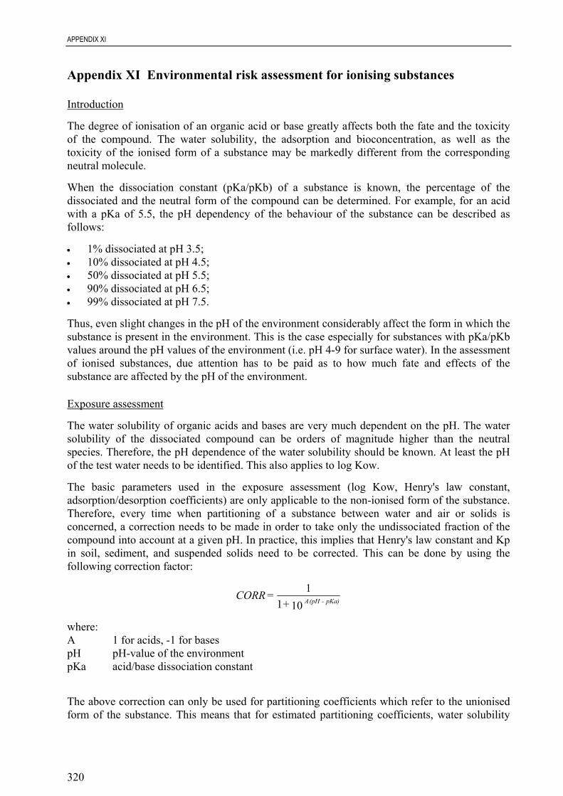
APPENDIX XI
320
Appendix XI Environmental risk assessment for ionising substances
Introduction
The degree of ionisation of an organic acid or base greatly affects both the fate and the toxicityof the compound. The water solubility, the adsorption and bioconcentration, as well as thetoxicity of the ionised form of a substance may be markedly different from the correspondingneutral molecule.
When the dissociation constant (pKa/pKb) of a substance is known, the percentage of thedissociated and the neutral form of the compound can be determined. For example, for an acidwith a pKa of 5.5, the pH dependency of the behaviour of the substance can be described asfollows:
• 1% dissociated at pH 3.5;• 10% dissociated at pH 4.5;• 50% dissociated at pH 5.5;• 90% dissociated at pH 6.5;• 99% dissociated at pH 7.5.
Thus, even slight changes in the pH of the environment considerably affect the form in which thesubstance is present in the environment. This is the case especially for substances with pKa/pKbvalues around the pH values of the environment (i.e. pH 4-9 for surface water). In the assessmentof ionised substances, due attention has to be paid as to how much fate and effects of thesubstance are affected by the pH of the environment.
Exposure assessment
The water solubility of organic acids and bases are very much dependent on the pH. The watersolubility of the dissociated compound can be orders of magnitude higher than the neutralspecies. Therefore, the pH dependence of the water solubility should be known. At least the pHof the test water needs to be identified. This also applies to log Kow.
The basic parameters used in the exposure assessment (log Kow, Henry's law constant,adsorption/desorption coefficients) are only applicable to the non-ionised form of the substance.Therefore, every time when partitioning of a substance between water and air or solids isconcerned, a correction needs to be made in order to take only the undissociated fraction of thecompound into account at a given pH. In practice, this implies that Henry's law constant and Kpin soil, sediment, and suspended solids need to be corrected. This can be done by using thefollowing correction factor:
1011
pKa) - (pH A + = CORR
where:A 1 for acids, -1 for basespH pH-value of the environmentpKa acid/base dissociation constant
The above correction can only be used for partitioning coefficients which refer to the unionisedform of the substance. This means that for estimated partitioning coefficients, water solubility

APPENDIX XI
321
and Kow need to be determined for the neutral form. The choice of relevant pH values to be usedin the calculation should be based on the pKa/pKb of the compound in concern and any relevantknowledge of the actual toxic form of the substance. For experimentally determined partitioncoefficients the need for correction should be assessed on a case by case basis, depending on thepH in the test.
These principles apply also to the fate of the substance in sewage treatment plant. However,since the STP is a well buffered environment, a default pH of 7 can be used in the calculations.The role of pH in the experimental determination of the bioconcentration should also beacknowledged.
Effects assessment
Ionisation can markedly alter the toxicity of the substance. Normally, this is caused by thedifferent bioavailability of the dissociated and neutral species. Consequently, when testingtoxicity, the tests should preferably be carried out at both sides of the pKa, to fully characterisethe possible differences in toxicity. Since this may not be possible in every case, the role of pHshould at least be discussed qualitatively in the assessment.
Risk characterisation
Care should be taken that the PEC and the PNEC in the risk characterisation represent similarconditions. PEC/PNEC comparisons should preferably be made at both sides of the pKa values,within environmentally relevant pH-range. The higher PEC/PNEC ratio should be used in therisk characterisation, following the realistic worst-case approach. If it is not possible to carry outa quantitative analysis, the assessor should take the pH effect into account qualitatively.

APPENDIX XII
322
Appendix XII Connection to Sweage Treatment Plants in Europe
Default STP Connection Rate
Marked improvements in overall EU wastewater collection (+22% relative to 1992) andtreatment (+69% relative to 1992) will follow full implementation of the Urban Waste WaterTreatment Directive (91/271/EEC) in 2005 (see Figure 1). Even before 2005, a provisionalfigure is indicated for interim use as substantial increases in wastewater collection (+12%) andtreatment (+40%) capacity have already been reported from across the EU. Projected wastewatertreatment capacity in the EU as a whole for 2000 is greater than baseline organic loadings (i.e.,106%), although this is not uniformly distributed throughout the EU. An interim figure of 80%connection to wastewater treatment is therefore proposed for the generic region. A figure of 90 -95% is also proposed for use following full implementation of the UWWTD. This coincides withthe likely ultimate degree of connection and treatment capacity for urban regions of the EU.
Figure 1. - Development in Collection and Treatment Capacity EU14 (Source: EC, 1999)10.
200,000
250,000
300,000
350,000
400,000
450,000
500,000
1992 1995 1998 2000 2005Year
1,00
0 p.
e.
Collection
Treatment
1992 Baseline Load
p.e. = person equivalent
Historical Data
Data on the proportion of the total population connected to wastewater treatment in individualMS in the period 1970-95 are presented in Table 1. The population weighted average for thewhole of the EU15 in 1995 was 73%. Although the apparent degree of connection to wastewatertreatment is low in some countries, its absence does not necessarily always imply inadequatetreatment or direct discharge. For example, the proportion of the population with individualarrangements such as septic tanks has been reported as 24% inGreece, 23% in France, 22% inFinland, 12% in Portugal, 7% in Germany, 6% in Italy, 2.5% in the UK, 1.5% in theNetherlands, 1% in Spain and 0.5% in Luxembourg (EWWG, 1997)
10 European Commission (1999). Implementation of Council Directive 91/271/EEC of 21 May 1991 concerning
urban waste water treatment as amended by Commission Directive 98/15/EC of 27 February 1998. Summary ofthe measures implemented by the member states and assessment of the information received pursuant to Article17 and 13 of the directive. Available on European Union (EU) web-site at http://www.europa.eu.int/water/water-urbanwaste/report/report.html.
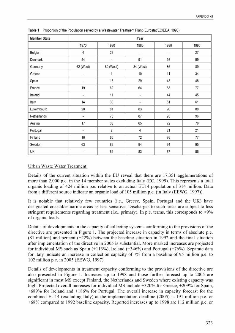
APPENDIX XII
323
Table 1 Proportion of the Population served by a Wastewater Treatment Plant (Eurostat/EC/EEA, 1998)
Member State Year
1970 1980 1985 1990 1995
Belgium 4 23 - - 27
Denmark 54 - 91 98 99
Germany 62 (West) 80 (West) 84 (West) 86 89
Greece - 1 10 11 34
Spain - 18 29 48 48
France 19 62 64 68 77
Ireland - 11 - 44 45
Italy 14 30 - 61 61
Luxembourg 28 81 83 90 88
Netherlands - 73 87 93 96
Austria 17 38 65 72 76
Portugal - 2 4 21 21
Finland 16 65 72 76 77
Sweden 63 82 94 94 95
UK - 82 83 87 86
Urban Waste Water Treatment
Details of the current situation within the EU reveal that there are 17,351 agglomerations ofmore than 2,000 p.e. in the 14 member states excluding Italy (EC, 1999). This represents a totalorganic loading of 424 million p.e. relative to an actual EU14 population of 314 million. Datafrom a different source indicate an organic load of 105 million p.e. (in Italy (EEWG, 1997)).
It is notable that relatively few countries (i.e., Greece, Spain, Portugal and the UK) havedesignated coastal/estuarine areas as less sensitive. Discharges to such areas are subject to lessstringent requirements regarding treatment (i.e., primary). In p.e. terms, this corresponds to <9%of organic loads.
Details of developments in the capacity of collecting systems conforming to the provisions of thedirective are presented in Figure 1. The projected increase in capacity in terms of absolute p.e.(81 million) and percent (+22%) between the baseline situation in 1992 and the final situationafter implementation of the directive in 2005 is substantial. More marked increases are projectedfor individual MS such as Spain (+113%), Ireland (+346%) and Portugal (+76%). Separate datafor Italy indicate an increase in collection capacity of 7% from a baseline of 95 million p.e. to102 million p.e. in 2005 (EEWG, 1997).
Details of developments in treatment capacity conforming to the provisions of the directive arealso presented in Figure 1. Increases up to 1998 and those further forecast up to 2005 aresignificant in most MS except Finland, the Netherlands and Sweden where existing capacity washigh. Projected overall increases for individual MS include +320% for Greece, +209% for Spain,+689% for Ireland and +186% for Portugal. The overall increase in capacity forecast for thecombined EU14 (excluding Italy) at the implementation deadline (2005) is 191 million p.e. or+68% compared to 1992 baseline capacity. Reported increases up to 1998 are 112 million p.e. or

APPENDIX XII
324
+40% compared to 1992. Increases to date in individual member states include +27% forGermany, +51% for France, +82% UK, +91% for Spain and +95% for Portugal. It has beenconcluded that by the implementation deadline, the capacity of the treatment plants would besufficient to treat the total projected combined organic load for agglomerations >2000 pe in allthe 14 EU MS (EC, 1999). Indeed, projected final treatment capacity (469 million p.e.) isapproximately 11% greater than the total organic load (424 million p.e.). However, distributionof treatment capacity will not necessarily be homogenous. For example, projected treatmentcapacity post-implementation exceeds 1992 baseline organic loads by +28% in the Netherlands,+35% in Germany and +74% in Sweden. Treatment capacity in Italy is forecast to increase by73% from a baseline of 59 million p.e. to 102 million p.e. in 2005 (EEWG, 1997).
APPENDIX XIII
325
Appendix XIII Risk assessment of sources not covered by the life-cycle of thesubstance
Introduction
Exposure may occur from other sources than the life-cycle of the produced or importedsubstance under assessment. Such sources have been referred to as “unintentional sources”.Examples are substances of natural origin, substances formed in combustion processes andindirect emissions of the substance, e.g. as by-product, contaminant or degradation product ofanother substance. In these cases information is necessary on emissions which are not coveredby the life-cycle of the substance being assessed.
Knowledge of the extent of the sources not covered by the life-cycle of the substance underreview is necessary for a full evaluation of the risks posed by the priority existing substance orbiocidal product. The information is needed for example for a correct interpretation of measuredenvironmental concentrations. The information is also required for an evaluation of the relativecontribution of the emissions of the substance under review to the overall risks posed by thesubstance through all possible sources. Such information might be relevant in the eventualdevelopment of a risk reduction strategy.
In this appendix some recommendations are given on how to deal with these kind of sources,based on the practical experience gained with the implementation of the ESR. There is still aneed for an EU decision on how to handle these cases at the time of revision of the TGD.
Legal background
The Existing Substances Regulation (EEC) 793/93 (ESR) requires that all information needed tocarry out the risk assessment of a priority substances is submitted to the rapporteur by theProducers and Importers of the substance. The risk assessment however is one of a selectedpriority substance, the sources of which can be from the produced and imported substance, butalso from other sources. Commission Regulation (EC) 1488/94 for example foresees that the riskassessment of a priority substance entails an exposure assessment which, in particular is toconsider the exposures resulting from the life-cycle of the produced and imported prioritysubstance, but need not do so exclusively. The Biocidal Products Directive (98/8/EC) (BPD)states that cumulation of effects from the biocidal products containing the same activesubstances shall be taken into account, where relevant, in the assessment of a biocidal activesubstance.
Recommendation for sources not covered by the life-cycle of the substance
The rapporteur should clearly list other sources, which can give rise to exposure by the substancebeing assessed. The risk assessment should include as much readily available information onthese sources as possible. Whether or not this information can be taken into account in the riskcharacterisation is dependent on the quantity and quality of the available information. If there isnot sufficient confidence in the available database to make a conclusion of concern/no concern,the risk assessment should be finalised with the conclusion “further information is needed”(Conclusion (i)).
If the emissions originate from the life-cycle of another substance that can be prioritised underthe ESR (i.e. a substance listed in EINECS), it is not required to take these sources into accountin the risk characterisation, as they can be covered by prioritising the other substance. If the
APPENDIX XIII
326
other substance is being assessed, then the risk assessment of the original substance must betaken into account in the risk assessment of the other substance.
If the emissions can not be covered by the ESR or BPD, the rapporteur is recommended to usethe available information on these emissions as far as possible to carry out a riskcharacterisation. In the case that “further information is needed” (Conclusion (i)), then, ingeneral, it can not be the obligation of the producers or importers of the substance underexamination to obtain such information.
For biocides, sources which include substances of natural origin or releases from other biocidaluses should be taken into account in the risk assessment. When it comes to cumulative effects ofa substance used also outside the scope of the BPD (e.g. in plant protection products) and mayberegulated with another Directive there is, at the time of revision of the TGD, still a need for acommon EU decision on how to handle such cases. Exclusion of other than only biocidal usesfrom the assessment causes difficulties, for example, when using monitoring data or comparingmeasured residue data with Maximum Residue Limits.

APPENDIX XIV
327
Appendix XIV Information on the difference in diversity between saltwaterand freshwater
The greater diversity of species in saltwaters11 compared to freshwaters has been recognised formany years. In the key work “The Seas”, Russell and Yonge (1928) state that “The sea is farricher in different forms of life than the land or freshwater, many groups of animals beingexclusively marine”. This view has been consolidated in other publications which have based thedifference on a number of factors including the fact that life originated in the seas and they havebeen well populated since the earliest fossil records (Tait, 1978).
The results below show recent comparative data on freshwater and saltwater species diversitygenerated for the Danish Environmental Protection Agency by the Zoological Museum and theDepartment of Evolutionary Biology at University of Copenhagen.
Taxonomic group No. of species Comments
Porifera 4,850 (150 in freshwater)
Ctenophora 50 (Exclusively marine)
Cnidaria 7,000 (Exclusively marine)
Tubellaria 2000 (1000 in freshwater)
Trematoda 6,000 (internal parasites) ------
Cestoda 3,500 (internal parasites) ------
Nemateans 900 (Predominantly marine)
Gastrotricha 150 (Marine and fresh water)
Nematoda 5,000 (15,000 described species in totalincluding parasites and terrestrial, marine
and freshwater forms)
Nematomorpha 4 (316 in freshwater)
Achantocephala 1,150 (internal parasites) -----
Kinorhyncha 150 (Exclusively marine)
Priapulida 17 (Exclusively marine)
Loricifera 100 (Exclusively marine)
Gnatostomolida 80 (Exclusively marine)
Rotifera 100 (1,400 in freshwater)
Polychata 5-10,000 (1000 in freshwater)
Oligochaeta ------ (Many species; mainly in freshwater)
Echinodermata 7,000 (Exclusively marine)
Brachiopoda 300 (Exclusively marine)
Echiura 140 (Exclusively marine)
Sipunculida 350 (Exclusively marine)
Pogonophora 120 (Exclusively marine)
Tardigrada (Taxonomic group discovered a few
11 Except those where there are extremes of environmental conditions

APPENDIX XIV
328
Taxonomic group No. of species Commentsdecades ago. A few hundred speciesknown from both terrestrial, fresh- and
marine water)
Arthropoda
Chelicerata
Merostomata 4 (Exclusively marine)
Pygnogonida 1,000 (Exclusively marine)
Insecta 400 (25-30000 in freshwater)
Crustacea (5-6000 in freshwater)
Entomostraca 10,100 (3000 in freshwater)
Malacostraca 19,000 (3000 in freshwater)
Mollusca
Gastropoda 19,000 (4000 in freshwater)
Bivalvia 5,450 (2,550 in freshwater)
Scaphopoda 350 (Exclusively marine)
Cephalopoda 600 (Exclusively marine)
Bryozoa 5,000 (70 in freshwater)
Hemichordata 100 (Exclusively marine)
Chordata
Tunicata 1,300 (Exclusively marine)
Cephalocordata 25 (Exclusively marine)
Vertebrata
Pisces 15,000 (Guestimate but believed to be anunderestimate number of freshwaterspecies less than number of marine
species)
Amphibians (Mainly freshwater)
Mammals 60 (Guestimate)
European Commission – Joint Research Centre Institute for Health and Consumer Protection European Chemicals Bureau (ECB) Technical Guidance Document on Risk Assessment in support of Commission Directive 93/67/EEC on Risk Assessment for new notified substances
Commission Regulation (EC) No 1488/94 on Risk Assessment for existing substances
Directive 98/8/EC of the European Parliament and of the Council concerning the placing of biocidal products on the market
Part II
The mission of the JRC is to provide customer-driven scientific and technical supportfor the conception, development, implementation and monitoring of EU policies. As aservice of the European Commission, the JRC functions as a reference centre ofscience and technology for the Union. Close to the policy-making process, it serves thecommon interest of the Member States, while being independent of special interests,private or national.
OFFICE FOR OFFICIAL PUBLICATIONS OF THE EUROPEAN COMMUNITIES L – 2985 Luxembourg