Part II - INCENTIVE RADIO LICENSE FEE CALCULATION MODEL
50
INTERNATIONAL TELECOMMUNICATION UNION TELECOMMUNICATION DEVELOPMENT BUREAU INCENTIVE RADIO LICENSE FEE CALCULATION MODEL by Dr. A.P. Pavliouk ITU/BDT Senior Expert on frequency management Bangkok 2000
Transcript of Part II - INCENTIVE RADIO LICENSE FEE CALCULATION MODEL
INTERNATIONAL TELECOMMUNICATION UNION TELECOMMUNICATION DEVELOPMENT BUREAU
INCENTIVE RADIO LICENSE FEE
CALCULATION MODEL
by Dr. A.P. Pavliouk
ITU/BDT Senior Expert on frequency management
Bangkok 2000
TABLE OF CONTENTS page
Introduction … ................................................................................................ 5
1 General Purpose of the Model ..................................................... 5
2 Steps in the Model Formulation ................................................... 6
3 General Principles for the Model Development............................ 7
4 Expenditures and Income of a State Concerning
Spectrum Management ............................................................... 8
5 Determination of the Used Spectral Resource Value................... 10
5.1 Determination of a Time Resource Used by an Emission............ 10
5.2 Determination of a Territorial Resource Used by an Emission..... 11
5.3 Determination of a Frequency Resource Used by an Emission... 13
5.4 Determination of Weighting Coefficients...................................... 13
5.5 Determination of the Whole Value of the Used Spectral Resource 15
6 Price for the Qualified Unit of the Used Spectral Resource ......... 15
7 Annual Fees for Particular Frequency Assignment...................... 16
ANNEX 1 Procedures and Examples of Used Spectral Resource
Calculations in Application to Different Radio Services ............... 17
A1.1 General Considerations ............................................................... 17
A1.2 Radio Broadcasting ..................................................................... 18
A1.2.1 VHF/UHF Sound and TV Radio Broadcasting ............................. 18
A1.2.1.1 Calculation Procedures................................................................ 18
A1.2.1.1.1 Service Area Radius Calculation ................................................. 18
A1.2.1.1.2 Effective Antenna Height Calculation........................................... 24
A1.2.1.1.3 Service Area Calculation ............................................................. 26
A1.2.1.2 Example of Calculations .............................................................. 29
A1.2.1.2.1 Incoming Parameters................................................................... 29
A1.2.1.2.2 Time and Frequency Resources Used ........................................ 29
A1.2.1.2.3 Territorial Resource Used............................................................ 29
A1.2.1.2.4 Spectral Resource Used.............................................................. 30
A1.2.2 LF - HF Sound Broadcasting ....................................................... 30
A1.3 Mobile Radio Services ................................................................. 32
A1.3.1 Land Mobile Radio Service.......................................................... 32
2
A1.3.1.1 Background of Calculation Procedures........................................ 32
A1.3.1.2 Calculation Procedures................................................................ 37
A1.3.1.3 Example of Calculations .............................................................. 37
A1.3.1.3.1 Incoming Parameters................................................................... 37
A1.3.1.3.2 Time and Frequency Resources Used ........................................ 37
A1.3.1.3.3 Territorial Resource Used............................................................ 37
A1.3.1.3.4 Spectral Resource Used.............................................................. 38
A1.3.2 Maritime Mobile Radio Service .................................................... 38
A1.3.2.1 Background of Calculation Procedures........................................ 38
A1.3.2.2 Calculation Procedures................................................................ 40
A1.3.2.3 Example of Calculations .............................................................. 40
A1.3.2.3.1 Incoming Parameters................................................................... 40
A1.3.2.3.2 Time and Frequency Resources Used ........................................ 41
A1.3.2.3.3 Territorial Resource Used............................................................ 41
A1.3.2.3.4 Spectral Resource Used.............................................................. 42
A1.3.3 Aeronautical Mobile, Radionavigation
and Radiolocation Services ......................................................... 42
A1.3.3.1 Calculation Procedures................................................................ 42
A1.3.3.2 Examples of Calculations............................................................. 43
A1.3.3.2.1 Aeronautical Radio Communications........................................... 43
A1.3.3.2.1.1 Incoming Parameters................................................................... 43
A1.3.3.2.1.2 Time and Frequency Resources Used ........................................ 43
A1.3.3.2.1.3 Territorial Resource Used............................................................ 43
A1.3.3.2.1.4 Spectral Resource Used.............................................................. 44
A1.3.3.2.2 Primary Radars............................................................................ 44
A1.3.3.2.2.1 Incoming Parameters................................................................... 44
A1.3.3.2.2.2 Time and Frequency Resources Used ........................................ 44
A1.3.3.2.2.3 Territorial Resource Used............................................................ 44
A1.3.3.2.2.4 Spectral Resource Used.............................................................. 45
A1.4 Fixed Radio Services................................................................... 45
A1.4.1 Calculation Procedures................................................................ 45
A1.4.2 Example of Calculations .............................................................. 46
A1.4.2.1 Incoming Parameters................................................................... 46
A1.4.2.2 Time and Frequency Resources Used ........................................ 46
3
A1.4.2.3 Territorial Resource Used............................................................ 47
A1.4.2.4 Spectral Resource Used.............................................................. 47
A1.5 Earth Stations of Satellite Communications................................. 47
A1.5.1 Calculation Procedures................................................................ 47
A1.5.2 Examples of Calculations............................................................. 48
A1.5.2.1 Transmitting Earth Station ........................................................... 48
A1.5.2.1.1 Incoming Parameters................................................................... 48
A1.5.2.1.2 Time and Frequency Resources Used ........................................ 48
A1.5.2.1.3 Territorial Resource Used............................................................ 48
A1.5.2.1.4 Spectral Resource Used.............................................................. 48
A1.5.2.2 Receiving Earth Station ............................................................... 49
A1.5.2.2.1 Incoming Parameters................................................................... 49
A1.5.2.2.2 Time and Frequency Resources Used ........................................ 49
A1.5.2.2.3 Territorial Resource Used............................................................ 49
A1.5.2.2.4 Spectral Resource Used.............................................................. 49
A1.6 Summary of Calculation Results.................................................. 50
4
Introduction
The Model was developed in the frameworks of the BDT Sub-regional (South-east Asia) Project on Spectrum Validation and Licensing, Bangkok, 2000. The study focuses on a specific method of spectrum fee calculation. The Model is derived from the conceptual base that there is a distinct need to price spectrum and that the pricing of spectrum resources should reflect more than administrative convenience. This has been reinforced by the views of administrations participating in the data collection and policy review of SE Asian countries under the above Project. The importance of the Model rests on it providing to administrations a functional tool which can be used to calculate spectrum fees on the basis of tangible criteria. In fact it falls within the category of administrative incentive pricing approaches that were documented in the ITU-R Report SM.2012-1. In the manner of most prevalent administrative incentive approaches it allows variations in not only the criteria used as inputs to the pricing but supports weighting those criteria to reflect the importance of certain spectrum utilization variables. This can also be used to vary the pricing between different spectrum uses whereby the underlying scarcity of spectrum can be considered. The Model, being rather complicated for manual calculations, is the most effective in application to atomised National Spectrum Management Systems. Relevant software can be customised in accordance with the Model and all the rest calculations will be fulfilled automatically without any involvement of the system operators. Similar experience is described by Administration of Kyrgyz Republic in Report SM.2012-1. 1 General Purpose of the Model The purpose of this Model is to increase spectrum utilisation efficiency. It is designed to introduce non-discriminatory access to the spectrum for various categories of users, stimulate the use of less congested (particularly – higher) frequency bands, stimulate harmonised development of radio communication services throughout the country, and cover the cost of spectrum management. It includes the consideration of the phased development and/or maintenance of spectrum management and monitoring facilities and reimbursement of expenditures of a national telecommunication Administration including its international activities within ITU. The Model was developed on the basis of materials (including those contributed by the authors of this Report) contained in the new version of Report ITU-R SM.2012 "Economic Aspects of Spectrum Management", which will be published soon as Report ITU-R SM.2012-1, and other available publications. The Model determines the value of annual payments to be made for the spectrum use of each transmitting radio station using a pricing formula based on the following basic elements:
5
• Three-dimensional radio frequency-spatial*-time resource, referred to as the spectral resource, used in the country and representing the common spectral value applicable to all frequency assignments, stored in the national Spectrum Management database and which is calculated on an annual basis.
• For each frequency assignment the spectral value is determined by the
frequency band occupied by the emission, multiplied by an area, occupied by the emission (which is determined by the power of transmitter, height and direction of the antenna etc.), and multiplied by the fraction of time throughout which the transmitter operates with that emission in accordance with terms of relevant license. Relevant assumptions and criteria are presented below in Section 5.
• The annual administration cost of spectrum management including the phased
development and/or maintenance of spectrum management and monitoring facilities and the reimbursement of expenditures of a national telecommunication Administration.
• The average price for the spectral resource unit determined from the above
values.
• The annual payment by a specific user determined from the actual value of used spectral resource.
A number of incentive weighting factors are entered in the formula. Thus the spectrum price or fee will depend not only on the relevant occupied bandwidth and coverage area values, but also on time-sharing conditions, geographical location of the station, economic development level or population density in the coverage area, social factors, exclusivity, type of radio service, spectrum employment, as well as some operational factors such as complexity of radio monitoring and imposing sanctions etc. The proposed Model allows the user at any moment to determine the value of his annual payment for the spectrum and also renders it to be transparent and accessible to all users. Thus, if the user employs greater bandwidth and service area, operates in more populated geographical area or the area is more economically developed and operates full time in more congested frequency bands, the larger will be the payment. The approach thus encourages more efficient spectrum use and is an incentive for the user to implement more modern equipment and operate in new higher frequency bands. It should also encourage the use if possible of time-sharing regimes with other users, avoid using redundant margins for the power of a transmitter and height of antenna etc. and support expansion of its coverage to rural and remote areas. * For reasons of simplicity and taking into account that spectrum sharing conditions are
usually provided only by territory separation of stations, for purposes of the given Model a spatial (three-dimensional) resource is represented by a territorial (two-dimensional) one.
6
2 Steps in the Model Formulation The proposed spectrum payment algorithm includes the following steps:
• Determination of annual expenditures of the state on management of actually used spectral resource and determination of the common value of the annual payments for all spectral resources.
• Determination of the value of the spectral resource used by each radio station
and, through their summation, by all stations registered in a national Spectrum Management Database.
• Determination of the price for a unit of the spectral resource.
• Determination of the annual payment for a specific user on a differential and
non-discriminatory basis, determined from the actual value of used spectral resource.
Each of these steps is described in detail below. 3 General Principles for the Model Development It is necessary to underline that the number and values of all particular coefficients below are given only as illustrative examples. They are based on available data and the experts estimations in application to South-East Asia countries. Each National Telecommunication Administration can chose other values and add other coefficients reflecting its particular needs and experiences. All coefficient values, unless indicated specifically, can be integer or fractional numbers. The Model is intended to cover those cases (and they are the great majority of frequency assignments) for which simplified calculation methods of some important parameters (mainly – service or occupied areas) can be used. This approach has been chosen also from the understanding that for purposes of fees calculation it is much more important to provide universal procedures to guarantee equal conditions for all users belonging to one group (by radio service or its particular application) rather than to obtain a high accuracy of technical parameter calculations. Different options in obtaining data necessary for calculations are presented in Annex 1 . Based on a general principal that not only a transmitter but also a receiver occupies a particular spectral resource by denying operation of other transmitters (other than a communicating one) in a particular frequency band within the limits of a particular territory (Recommendation ITU-R SM.1046-1), the Model can be used for calculating fees for receivers as well in a case when a user requires protection of a receiver from interference and it is registered in a National Frequency Assignment Database. The procedures for the calculations are presented in Annex 1.
7
Annex 1 also presents some options to Administrations on simplification of calculations procedures, followed by decreasing of calculation accuracy, or on their somewhat complication for increasing calculation accuracy. For some new radio systems for which the service area or occupied frequency band calculations are very complicated and when they have not been definitively fixed (spread-spectrum systems, satellite mobile communications using LEO, MEO etc.), calculations can be postponed and fixed license fee regimes could continued to be used. 4 Expenditures and Income of a State Concerning Spectrum Management This Section considers the basis on which the state or administrations costs for spectrum management could be considered. The total amount of the annual payments for spectral resource Can, to be collected from all users, can be presented as: Can = C1 + C2 - Ian (units of a national currency) (1) where:
C1: share of the sum that is necessary for covering expenditures of the state on all national and international spectrum management activities
C2: net income of the state, if applied
Ian: total amount of annual radio communication inspection charges, if
applied. The last term is applied if an Administration uses separate additional tariffs for inspection and examination activities (examination of frequency assignment application forms, inspection of radio stations after installations before entering to operation, systematic inspection of radio installations on conformity to license terms, etc.). This value can be assumed for each current year based on previous year data.
It is possible to subdivide the terms C1 and C2 into additional components: C1 = C11 + C12 + C13 + C14 (2) where:
C11: funds necessary for the purchase and efficient operations using spectrum management system facilities and equipment, including radio monitoring station equipment, direction finders, computers and software for monitoring stations and for a national Spectrum Management Database, equipment for inspection purposes, materials, amortisation of buildings, constructions, transport vehicles, etc.
8
C12: funds necessary for carrying out supporting scientific research, purchase of the scientific and operational literature, international standards and recommendations, carrying out electromagnetic compatibility analysis for supporting frequency assignment process, etc.
C13: funds necessary to provide efficient activities of a national
telecommunication Administration within ITU-R and to fulfil bilateral and multilateral frequency co-ordination obligations relating to terrestrial and satellite radio services etc.
C14: spectrum management staff salaries.
Taxes are not included in the amounts C11 - C14. Coefficient C2 can be presented as the following components: C2 = C21 + C22, (3) where:
C21: taxes on the incomes of a national spectrum management body and taxes included in the cost of the equipment, software, materials etc., which are bought by this body from the market
C22: additional payment for spectrum use coming directly to a state budget.
To encourage faster development of radio communication services to support economic development of a country some countries do not apply such additional charges (see Report ITU-R SM.2012-1). Formulas (1) and (3) do not take into account any indirect income of the state from the used spectral resource in the form of taxes from the incomes of the telecommunication operators whose activity is connected with spectral resource use (for example, taxes from the incomes of the cellular communication operators). This component of the income of the state usually is collected and repeatedly exceeds reasonable values of C22, if those would be collected. At the same time these taxes are also the state income from used spectral resource although an indirect one. In essence C22 is some kind of advanced payment to the state for a spectrum and many telecommunication operators, especially in the developing countries, will not be immediately be able to make such large payments and furthermore this could be an obstacle to development. A good measure of the provision of an economic incentive is to reduce to a minimum the C22 component, so that a telecommunication operator begins to provide service as quickly as possible. The loss of this C22 component can be easily compensated by a state from taxes from the telecommunication operator’s activity.
9
Thus, for the purposes of rapid development of telecommunications and information services in a country and the creation of economic incentives to the telecommunication operators, it is essential to hold spectrum payments to the minimum necessary values to cover the costs of a national spectrum management. Administrations can gain further fees from the license for applications to which the spectrum is used and furthermore the taxes on operator revenues will compensate for the revenue foregone. This will be the case particularly where spectrum fees and licensing are treated separately. 5 Determination of the Used Spectral Resource Value Proceeding from formulas (1) - (3) it is possible to determine Can. representing the cumulative annual expenditures and income payment for all spectral resources, used in the country. The second step is to determine the spectral resource value used by each user and then – by all users. These are calculated on the basis of data regarding each frequency assignment contained in a national Spectrum Management Database. The method proposed is as follows. For any i-th frequency assignment (from their total amount n incorporated in the national database) the three-dimensional value of the spectral resource, denoted as Wi, is to be determined as follows: Wi = α i ⋅ βi ⋅ (Fi ⋅ Si ⋅ Ti) (4)
where for i-th frequency assignment:
Fi: frequency resource
Si: territorial resource
Ti: time resource α I: aggregate coefficient which takes into account a number of weighting
factors, such as commercial, social and operational ones as it is given below
βI: weighting coefficient which determines exclusiveness of the frequency
assignment as it is given below. Let us consider items of formula (4) in their reverse order. 5.1 Determination of a Time Resource Used by an Emission A time resource Ti used by i -th emission is determined as: Ti ≤ 1 (year) (5)
10

and for each frequency assignment represents a fraction of time related to one year, determined in that or another way, during which the radio transmitter operates in accordance with terms set out in the relevant license. It can be a fraction of a day, which may be the case with broadcasting or PMR service, or a fraction of a year for seasonal operations such as expeditions, agricultural activities etc. For example, if particular TV transmitter in accordance with terms of its license is operating only 16 hours per a day throughout the whole year, than: Ti = 16/24 = 0.67 year. If another transmitter (for example an HF one used for geological expedition), in accordance with terms of its license can operate totally only 3 month per a year, than: Ti = 3/12 = 0.35 year. It is obvious that for a transmitter which operates permanently, for example a microwave (RRL) one (short intervals of maintenance breaks usually do not taken into account if it is not especially stated in the license), Ti = 1 year. The last situation is usually typical for the majority of frequency assignments presented in any national Spectrum Management Database. Such a regime is the most commonly requested and licensed. 5.2 Determination of a Territorial Resource Used by an Emission A territorial resource Si used by i -th emission is determined as: Si = bij ⋅ si (km2) (6) 1 m ≤≤ j where:
si: the territory actually occupied ( covered) by the emission in accordance with certain criteria, km2
bij: weighting coefficient which depends on the j -th category of the territory
actually occupied by the emission
m: number of categories.
The number of categories m and the relevant values of the weighting coefficients bj should be set out by a National Telecommunications Administration. These categories can take into account density of population and/or level of economic (industrial and/or agricultural) development of various regions of a country. It represents a measure of attractiveness for radio communication and broadcasting operators. Categories may also distinguish urban and rural areas, inland and coastal areas, mainland and island areas. Additionally settlement type and number of permanent or transitory inhabitants could also be included. Illustrative examples are presented in Table 1.
11
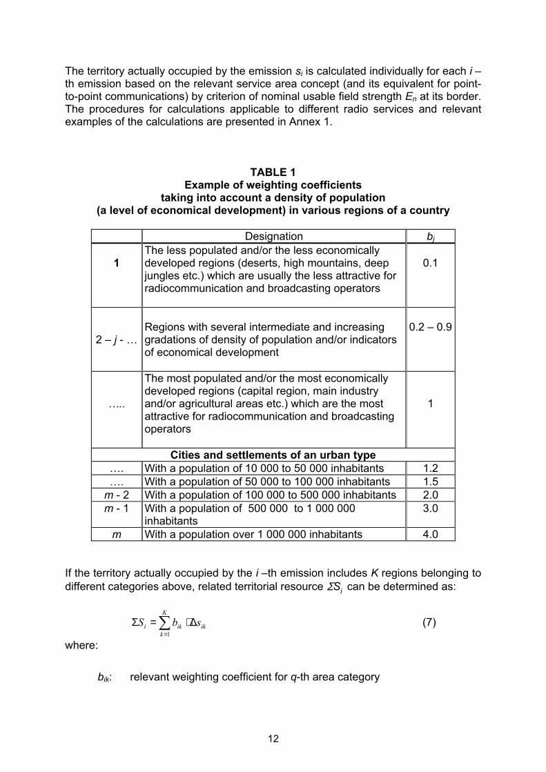
The territory actually occupied by the emission si is calculated individually for each i –th emission based on the relevant service area concept (and its equivalent for point-to-point communications) by criterion of nominal usable field strength En at its border. The procedures for calculations applicable to different radio services and relevant examples of the calculations are presented in Annex 1.
TABLE 1
Example of weighting coefficients taking into account a density of population
(a level of economical development) in various regions of a country
Designation bj 1
The less populated and/or the less economically developed regions (deserts, high mountains, deep jungles etc.) which are usually the less attractive for radiocommunication and broadcasting operators
0.1
2 – j - …
Regions with several intermediate and increasing gradations of density of population and/or indicators of economical development
0.2 – 0.9
…..
The most populated and/or the most economically developed regions (capital region, main industry and/or agricultural areas etc.) which are the most attractive for radiocommunication and broadcasting operators
1
Cities and settlements of an urban type …. With a population of 10 000 to 50 000 inhabitants 1.2 …. With a population of 50 000 to 100 000 inhabitants 1.5
m - 2 With a population of 100 000 to 500 000 inhabitants 2.0 m - 1 With a population of 500 000 to 1 000 000
inhabitants 3.0
m With a population over 1 000 000 inhabitants 4.0 If the territory actually occupied by the i –th emission includes K regions belonging to different categories above, related territorial resource ΣSi can be determined as:
∑=
∆⋅=ΣK
kikiki sbS
1 (7)
where:
bik: relevant weighting coefficient for q-th area category
12
sik: relevant proportion of the whole occupied region si, i.e.
∑=
∆=K
kiki ss
1.
Usually 1≤ 3. ≤k Examples for the calculation of proportional values sik for different cases are presented in Annex 1 (Section A1.2.1.1.3). If an Administration has a digital administrative terrain database interrelated with relevant frequency assignment software, calculations of ΣSi can be made automatically in accordance with a procedure presented in Section 5.2.6 of Report ITU-R SM. 2012-1. 5.3 Determination of a Frequency Resource Used by an Emission A frequency resource Fi used by i -th emission is determined as: Fi = χ Bni (MHz) (8) where:
Bni necessary bandwidth of the emission in MHz, calculated in accordance with Recommendation ITU-R SM.1138 (see Radio Regulations, Geneva 1998, Volume 4), taking into account that an occupied bandwidth of an emission should be equal to its necessary bandwidth (Recommendation ITU-R SM. 328-9)
χ : adjustment factor ( 0 ≤≤ χ 1) can be used in some cases, for example,
to decrease somewhat a very great difference in fees between sound and TV broadcasting, under the same powers of transmitters, due to significant difference in the necessary bandwidths. It also can be used in cases of radar applications (see example of calculations below) etc..
5.4 Determination of Weighting Coefficients General weighing coefficient α i in formula (4) can be presented as a product of the following fractional coefficients:
α i = α1⋅ α2 ⋅ α3 ⋅ α4 ⋅ α5 (9) where:
α1: takes into account commercial value of the spectrum range used α2: taking into account social factor α3: takes into account features of transmitter location
13
α4: takes into account the complexity of spectrum management functions α5: other coefficient (coefficients) which can be introduced by an
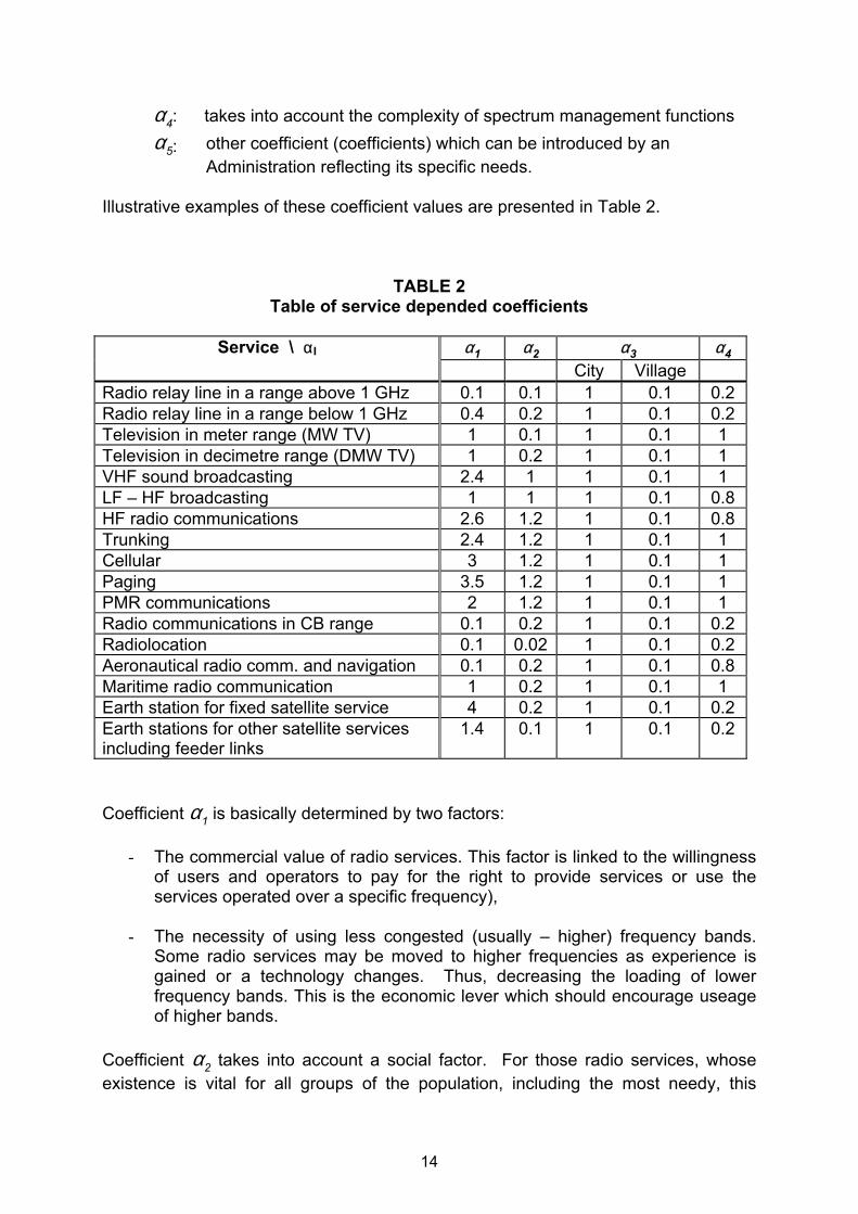
Administration reflecting its specific needs. Illustrative examples of these coefficient values are presented in Table 2.
TABLE 2 Table of service depended coefficients
Service \ αI α1 α2 α3 α4
City Village Radio relay line in a range above 1 GHz 0.1 0.1 1 0.1 0.2 Radio relay line in a range below 1 GHz 0.4 0.2 1 0.1 0.2 Television in meter range (MW TV) 1 0.1 1 0.1 1 Television in decimetre range (DMW TV) 1 0.2 1 0.1 1 VHF sound broadcasting 2.4 1 1 0.1 1 LF – HF broadcasting 1 1 1 0.1 0.8 HF radio communications 2.6 1.2 1 0.1 0.8 Trunking 2.4 1.2 1 0.1 1 Cellular 3 1.2 1 0.1 1 Paging 3.5 1.2 1 0.1 1 PMR communications 2 1.2 1 0.1 1 Radio communications in CB range 0.1 0.2 1 0.1 0.2 Radiolocation 0.1 0.02 1 0.1 0.2 Aeronautical radio comm. and navigation 0.1 0.2 1 0.1 0.8 Maritime radio communication 1 0.2 1 0.1 1 Earth station for fixed satellite service 4 0.2 1 0.1 0.2 Earth stations for other satellite services including feeder links
1.4 0.1 1 0.1 0.2
Coefficient α1 is basically determined by two factors:
- The commercial value of radio services. This factor is linked to the willingness of users and operators to pay for the right to provide services or use the services operated over a specific frequency),
- The necessity of using less congested (usually – higher) frequency bands.
Some radio services may be moved to higher frequencies as experience is gained or a technology changes. Thus, decreasing the loading of lower frequency bands. This is the economic lever which should encourage useage of higher bands.
Coefficient α2 takes into account a social factor. For those radio services, whose existence is vital for all groups of the population, including the most needy, this
14
coefficient has a low value reflecting a truly social value or obligation on behalf of the Administration. For example, for stations above 1 GHz, through which long-distance communications are provided, as well as for television broadcasting, the coefficient α2 has a low value and for cellular communication, coefficient α2 has a higher value. Coefficient α3 takes into account features of site location in urban and village conditions. In village conditions, where the density of the population is low and the level of the incomes is also low, the commercial value of communication services will also be low, at the same time technological costs for providing these services will also be high. Therefore with the purpose of support of the telecommunication operators and services as well as for encouraging development of radio communication services this can be a lower coefficient α3, while in urban districts it may be considerably higher. Coefficient α4 is determined by the complexity of spectrum management functions performed. This coefficient is usually the highest for mobile services. It is here that it is required to carry out the function of radio determination of mobile objects. Likewise for television broadcasting, it is required to determine with a high degree of accuracy a number of relevant parameters. Another weighting coefficient in formula (4) is βi. This coefficient determines exclusiveness of the frequency assignment. If, the given site of the spectrum is used on an exclusive basis, then βi = 1. With sharing βi varies within the limits from 0 up to 1 depending on conditions of sharing. Sharing may be on the basis of territorial separation that can result in reducing actual service area etc. 5.5 Determination of the Whole Value of the Used Spectral Resource Thus, with the help of weighting coefficients bj, αi and βi in accordance with formula (4), it is possible to determine (in view of the various factors) spectral resource Wi actually used for each frequency assignment. Then it is possible to determine the whole value of spectral resource W used in the country, according to the formula:
∑=
=n
jjWW
1 (MHz ⋅ km2 ⋅ 1 year) (10)
where:
Wi: spectral resource used by i-th frequency assignment n: overall number of frequency assignments registered in the national
Spectrum Management Database.
15

6 Price for the Qualified Unit of the Used Spectral Resource On the basis of the formulas (1) - (3) the total amount of annual payment can be determined which should be received from all users of all or part of the spectral resource. This could be done for all users combined or for individual services such as mobile cellular or broadcasting. On the basis of the formulas (4) – (10) the whole value of the annually used spectral resource in the country can be determined. Then it is possible to determine the price of ∆Can for a qualified unit of the spectral resource: ∆Can = L (Can / W) (units of a national currency / MHz ⋅ km2 ⋅ 1 year) (11) where:
L: adjustment factor which takes into account possible changes in prices costs in the country for the next fiscal year.
7 Annual Fees for Particular Frequency Assignment According to formula (11) the price ∆Can for the qualified unit of the spectral resource is determined. Formula (4) gives the value of the spectral resource Wi used for a particular i-th frequency assignment. Based on this, the amount of the annual payment Ci from the specific user of the spectrum for this frequency assignment will be determined as:
Ci = ∆Can ⋅ Wi (12) If the particular radio communication operator has several frequency assignments, the payment for each assignment is determined as above and then they are summated in relation to all operator's frequency assignments.
16
ANNEX 1
PROCEDURES AND EXAMPLES OF USED SPECTRAL RESOURCE
CALCULATIONS IN APPLICATION TO DIFFERENT RADIO SERVICES A1.1 General Considerations It is necessary to stress that calculation methods and procedures of service occupied areas, fixed radio link lengths etc. for exact operational purposes are usually very complicated, time consuming and require special qualification of the personnel. Their implementation for license fee calculation purposes could impose a great additional workload on a national spectrum management staff and not lead to significant increasing accuracy of such kind of calculations. Moreover, for the purposes of fee calculations it is much more important to provide universal procedures to guarantee equal conditions for all users belonging to one group (by radio service or its particular application) rather than to have a high accuracy of technical parameter calculations. Taking this into account, for purposes of the given license fees calculation Model, considerably simplified calculation methods are proposed. The main orientation is given on using pre-calculated graphs and tables rather than complicated formulas. For the most difficult cases (HF broadcasting, satellite communications etc.) particular calculations of service areas, fixed radio link lengths etc. can be replaced by values taken directly from relevant license application forms or received from operators by special requests. Another common approach is to make estimation of service or occupied areas only within the national borders of a country. For maritime services national maritime economical border concept may be used (usually 200 miles, i.e. 360 km). For cellular mobile radio communication systems, paging etc. which may contain numerous base stations including micro- and pico-cell ones for nearby and indoor operations, it may be too time-consuming to make calculations based on the determination of service areas of individual base stations. Therefore for this case the overall service area of the relevant cellular network and overall frequency bands assigned for base-mobile and mobile-base communications can be used for calculation of a spectral resource, used by the whole network. Occupied areas of Earth stations of Satellite Communication Systems are proposed to be determined on the basis of coordination distances agreed during the process of coordination and notification of frequency and orbital assignments in the ITU-R. If these are not available a universal coordination distances of 350 km for VSAT-s and 750 km for other stations are proposed to be used. In some cases values agreed between Administration and operator can also be used. It was indicated in Section 3 above that the Model is also applicable to receivers for which users especially demand protection from interference. To calculate relevant
17
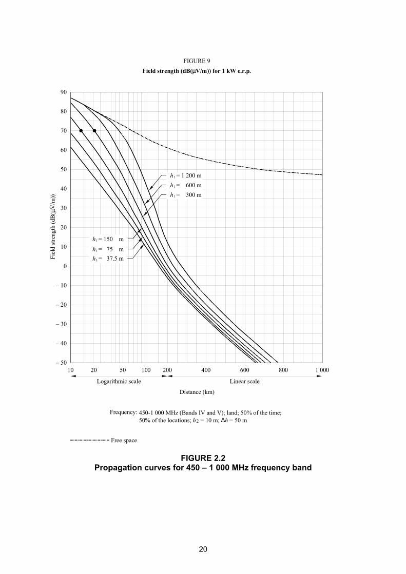
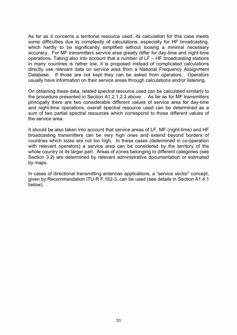
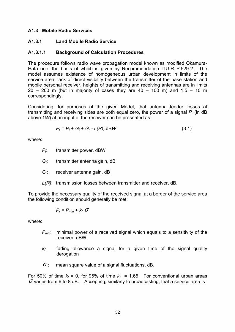
fees, in accordance with the principal of reciprocity of a receiver and transmitter, the receiver is substituted by a transmitter with a typical power (or a power agreed with the user) and antenna, which effective height, gain and direction correspond to the receiving one. For this set of parameters relevant spectral resource and then radio license fees are calculated in accordance with procedures presented below for related radio services and their applications. It is necessary to mention that an Administration, depending on particular conditions and abilities, may decide on simplification of some proposed calculation procedures. Particularly it concerns eliminating of service/occupied area subdivisions to different zones belonging to different license fees categories (see section A1.2.1.1.3) and the only one category, corresponding to the largest service/occupied area, can be used. It also concerns eliminating of the effective antenna height determinations (see section A1.2.1.1.2) etc. A1.2 Radio Broadcasting A1.2.1 VHF/UHF Sound and TV Radio Broadcasting A1.2.1.1 Calculation Procedures A1.2.1.1.1 Service Area Radius Calculation In the absence of digital terrain map facilities and computerized propagation and frequency planning models, which can provide exact automatic calculations, it is proposed to use the following simplified method of service area determination. The procedure is mainly based on provisions of Recommendation ITU-R P. 370-7 which presents propagation curves and procedures of their use for determining distances at which field strengths take specific values adopted as minimal usable by Recommendation ITU-R BT.417-4. The propagation curves presented at Figures 2.1 and 2.2 (Figures 1a and 9 of Recommendation ITU-R P. 370-7 correspondingly) represent field-strength values in VHF and UHF bands in dB( µ V/m) as a function of various parameters and refer to land paths. The propagation curves relate to transmitter power of 1 kW radiated from a half-wave dipole and represent the field-strength values exceeded at 50% of the locations (within any area of approximately 200 m by 200 m) for 50% of time. These field-strength values are usually used for service areas determination. They also correspond to different transmitting antenna heights and a receiving antenna height of 10 m. The curves are given for effective transmitting antenna heights between 37.5 m and 1 200 m, each value given of the “effective height” being twice that of the previous one. For different values of effective height, a linear interpolation between the two curves corresponding to effective heights immediately above and below the true value can be used. The curves are presented for the case when parameter, representing terrain irregularity, equals 50 m, i.e. corresponds to usual rolling terrain. For purposes of the given licence fees calculation Model it is proposed to use these curves also for other types of a terrain.
18
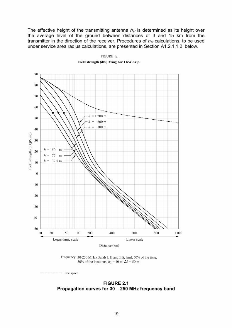
The effective height of the transmitting antenna hef is determined as its height over the average level of the ground between distances of 3 and 15 km from the transmitter in the direction of the receiver. Procedures of hef calculations, to be used under service area radius calculations, are presented in Section A1.2.1.1.2 below.
10 20 50 1 000100 200 400 600 800
90
80
70
60
50
40
30
20
10
0
– 10
– 20
– 30
– 40
– 50
h = 150 m1
h = 75 m1
h = 1 200 m1
h = 600 m1
h = 300 m1
h = 37.5 m 1
FIGURE 1aField strength (dB(µV/m)) for 1 kW e.r.p.
Fiel
d st
reng
th (d
B( µ
V/m
))
Logarithmic scale Linear scale
Distance (km)
Free space
2
30-250 MHz (Bands I, II and III); land; 50% of the time;50% of the locations; h = 10 m; ∆h = 50 m
Frequency:
FIGURE 2.1 Propagation curves for 30 – 250 MHz frequency band
19
10 20 50 200100 1 000800600400
90
80
70
60
40
30
20
10
0
– 10
– 20
– 30
– 40
– 50
50
h = 150 m1
h = 75 m1
h = 600 m1
h = 300 m1
h = 1 200 m1
h = 37.5 m1
FIGURE 9Field strength (dB(µV/m)) for 1 kW e.r.p.
Fiel
d st
reng
th (d
B( µ
V/m
))
Logarithmic scale Linear scale
Distance (km)
Free space
Frequency:2
450-1 000 MHz (Bands IV and V); land; 50% of the time;50% of the locations; h = 10 m; ∆h = 50 m
FIGURE 2.2 Propagation curves for 450 – 1 000 MHz frequency band
20
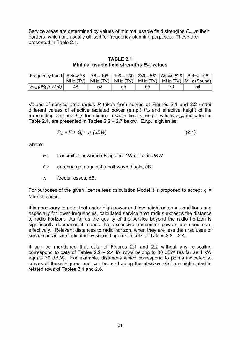
Service areas are determined by values of minimal usable field strengths Emu at their borders, which are usually utilised for frequency planning purposes. These are presented in Table 2.1.
TABLE 2.1 Minimal usable field strengths Emu values
Frequency band Below 76
MHz (TV) 76 – 108 MHz (TV)
108 – 230 MHz (TV)
230 – 582 MHz (TV)
Above 528 MHz (TV)
Below 108 MHz (Sound)
Emu (dB( µ V/m)) 48 52 55 65 70 54 Values of service area radius R taken from curves at Figures 2.1 and 2.2 under different values of effective radiated power (e.r.p.) Pef and effective height of the transmitting antenna hef, for minimal usable field strength values Emu indicated in Table 2.1, are presented in Tables 2.2 – 2.7 below. E.r.p. is given as: Pef = P + Gt + η (dBW) (2.1) where:
P: transmitter power in dB against 1Watt i.e. in dBW Gt: antenna gain against a half-wave dipole, dB η feeder losses, dB.
For purposes of the given licence fees calculation Model it is proposed to accept η = 0 for all cases. It is necessary to note, that under high power and low height antenna conditions and especially for lower frequencies, calculated service area radius exceeds the distance to radio horizon. As far as the quality of the service beyond the radio horizon is significantly decreases it means that excessive transmitter powers are used non-effectively. Relevant distances to radio horizon, when they are less than radiuses of service areas, are indicated by second figures in cells of Tables 2.2 – 2.4. It can be mentioned that data of Figures 2.1 and 2.2 without any re-scaling correspond to data of Tables 2.2 – 2.4 for rows belong to 30 dBW (as far as 1 kW equals 30 dBW). For example, distances which correspond to points indicated at curves of these Figures and can be read along the abscise axis, are highlighted in related rows of Tables 2.4 and 2.6.
21
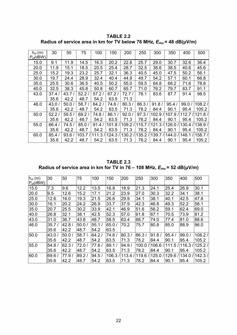
TABLE 2.2
Radius of service area in km for TV below 76 MHz, Emu = 48 dB(µV/m)
hef (m) Pef(dBW)
30 50 75 100 150 200 250 300 350 400 500
15.0 9.1 11.9 14.5 16.3 20.2 22.8 25.7 29.0 30.7 32.6 36.4 20.0 11.9 15.1 18.5 20.5 25.4 28.7 32.5 36.6 38.5 40.6 45.6 25.0 15.2 19.3 23.2 25.7 32.1 36.3 40.5 45.0 47.5 50.2 56.1 30.0 19.7 24.4 28.9 32.4 40.4 44.9 49.7 54.2 57.1 60.1 66.8 35.0 25.5 30.6 36.5 40.5 50.2 55.0 59.5 64.8 68.2 71.6 78.8 40.0 32.5 38.3 45.8 50.8 60.7 65.7 71.0 76.2 79.7 83.7 91.1 43.0 37.4 /
35.6 43.7 / 42.2
52.2 / 48.7
57.2 / 54.2
67.2 / 63.5
72.7 / 71.3
78.1 83.6 87.7 91.4 98.5
46.0 43.0 / 35.6
50.0 / 42.2
58.7 / 48.7
64.2 / 54.2
74.6 / 63.5
80.3 / 71.3
86.3 / 78.2
91.8 / 84.4
95.4 / 90.1
99.0 / 95.4
108.2 / 105.2
50.0 52.2 / 35.6
59.5 / 42.2
69.2 / 48.7
74.8 / 54.2
86.1 / 63.5
92.0 / 71.3
97.3 / 78.2
102.9 / 84.4
107.9 / 90.1
112.7 / 95.4
121.8 / 105.2
55.0 66.4 / 35.6
74.5 / 42.2
85.0 / 48.7
91.4 / 54.2
101.8 / 63.5
109.2 / 71.3
115.7 / 78.2
121.3 / 84.4
126.0 / 90.1
130.4 / 95.4
138.9 / 105.2
60.0 85.4 / 35.6
93.6 / 42.2
103.7 / 48.7
111.3 / 54.2
124.3 / 63.5
130.2 / 71.3
135.2 / 78.2
139.7 / 84.4
144.0 / 90.1
148.1 / 95.4
158.7 / 105.2
TABLE 2.3 Radius of service area in km for TV in 76 – 108 MHz, Emu = 52 dB(µV/m)
hef (m) Pef(dBW)
30 50 75 100 150 200 250 300 350 400 500
15.0 7.3 9.6 12.2 13.5 16.8 18.9 21.3 24.1 25.4 26.9 30.1 20.0 9.5 12.6 15.2 17.1 21.2 23.9 27.0 30.3 32.2 34.1 38.1 25.0 12.6 16.0 19.3 21.5 26.6 29.9 34.1 38.1 40.1 42.5 47.8 30.0 16.1 20.2 24.2 26.9 33.7 37.9 42.3 46.8 49.3 52.2 58.1 35.0 20.7 25.5 30.2 33.9 42.1 46.9 51.6 56.2 59.1 62.4 69.0 40.0 26.8 32.1 38.1 42.5 52.3 57.0 61.8 67.1 70.5 73.9 81.2 43.0 31.0 36.7 43.8 48.7 58.5 63.4 68.7 74.0 77.4 81.0 88.6 46.0 35.7 /
35.6 42.8 / 42.2
50.0 / 48.7
55.1 / 54.2
65.0 / 63.5
70.2 75.7 80.8 85.0 88.9 96.0
50.0 43.0 / 35.6
50.0 / 42.2
58.7 / 48.7
64.2 / 54.2
74.6 / 63.5
80.3 / 71.3
86.3 / 78.2
91.8 / 84.4
95.4 / 90.1
99.0 / 95.4
108.2 / 105.2
55.0 54.8 / 35.6
62.3 / 42.2
72.0 / 48.7
77.6 / 54.2
89.1 / 63.5
94.9 / 71.3
100.0 / 78.2
106.6 / 84.4
111.5 / 90.1
116.3 / 95.4
125.2 / 105.2
60.0 69.6 / 35.6
77.9 / 42.2
89.2 / 48.7
94.5 / 54.2
106.3 / 63.5
113.4 / 71.3
119.6 / 78.2
125.0 / 84.4
129.6 / 90.1
134.0 / 95.4
142.3 / 105.2
22
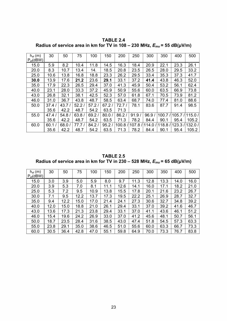
TABLE 2.4 Radius of service area in km for TV in 108 – 230 MHz, Emu = 55 dB(µV/m)
hef (m)
Pef(dBW) 30 50 75 100 150 200 250 300 350 400 500
15.0 5.9 8.2 10.4 11.8 14.5 16.3 18.4 20.9 22.1 23.3 26.1 20.0 8.3 10.7 13.4 14. 18.5 20.8 23.5 26.5 28.0 29.5 33.2 25.0 10.6 13.8 16.8 18.8 23.3 26.2 29.5 33.4 35.3 37.3 41.7 30.0 13.9 17.6 21.2 23.6 29.1 33.1 37.2 41.4 43.8 46.3 52.0 35.0 17.9 22.3 26.5 29.4 37.0 41.3 45.9 50.4 53.2 56.1 62.4 40.0 23.1 28.0 33.3 37.2 45.9 50.9 55.6 60.0 63.5 66.9 73.8 43.0 26.8 32.1 38.1 42.5 52.3 57.0 61.8 67.1 70.5 73.9 81.2 46.0 31.0 36.7 43.8 48.7 58.5 63.4 68.7 74.0 77.4 81.0 88.6 50.0 37.4 /
35.6 43.7 / 42.2
52.2 / 48.7
57.2 / 54.2
67.2 / 63.5
72.7 / 71.3
78.1 83.6 87.7 91.4 98.5
55.0 47.4 / 35.6
54.8 / 42.2
63.8 / 48.7
69.2 / 54.2
80.0 / 63.5
86.2 / 71.3
91.9 / 78.2
96.9 / 84.4
100.7 / 90.1
105.7 / 95.4
115.0 / 105.2
60.0 60.1 / 35.6
68.0 / 42.2
77.7 / 48.7
84.2 / 54.2
95.2 / 63.5
100.8 / 71.3
107.8 / 78.2
114.0 / 84.4
118.8 / 90.1
123.3 / 95.4
132.0 / 105.2
TABLE 2.5 Radius of service area in km for TV in 230 – 528 MHz, Emu = 65 dB(µV/m)
hef (m)
Pef(dBW) 30 50 75 100 150 200 250 300 350 400 500
15.0 3.0 3.9 5.0 5.9 8.0 9.7 11.3 12.8 13.3 14.0 16.0 20.0 3.9 5.3 7.0 8.1 11.1 12.6 14.1 16.0 17.1 18.2 21.0 25.0 5.3 7.2 9.5 10.9 13.8 15.5 17.8 20.1 21.6 23.2 26.7 30.0 7.1 9.5 12.2 13.7 17.3 19.5 22.2 25.1 26.9 28.7 32.7 35.0 9.4 12.2 15.0 17.0 21.4 24.1 27.3 30.6 32.7 34.8 39.2 40.0 12.0 15.0 18.8 21.0 26.1 29.4 33.1 37.0 39.2 41.6 46.7 43.0 13.6 17.3 21.3 23.8 29.4 33.1 37.0 41.1 43.6 46.1 51.2 46.0 15.4 19.6 24.2 26.9 33.0 37.0 41.2 45.6 48.1 50.7 56.1 50.0 18.7 23.5 28.4 31.6 38.5 43.0 47.4 51.8 54.5 57.3 63.3 55.0 23.8 29.1 35.0 38.6 46.5 51.0 55.6 60.0 63.3 66.7 73.3 60.0 30.5 36.4 42.8 47.0 55.1 59.8 64.9 70.0 73.3 76.7 83.8
23
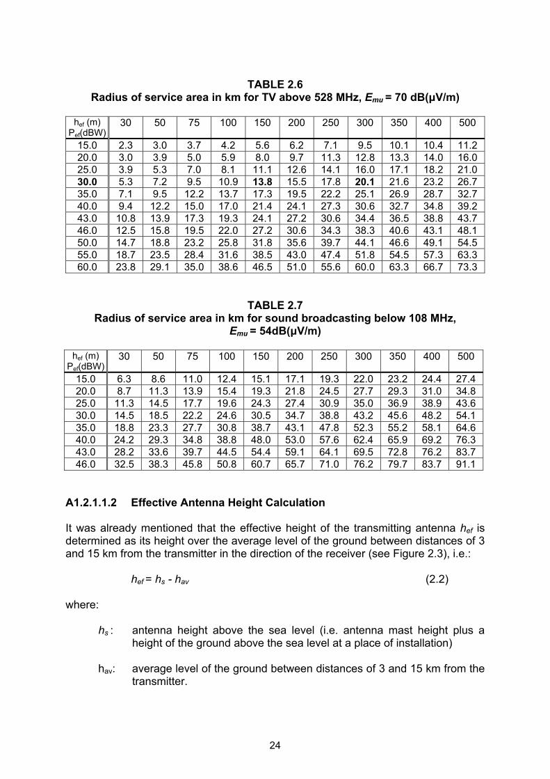
TABLE 2.6
Radius of service area in km for TV above 528 MHz, Emu = 70 dB(µV/m)
hef (m) Pef(dBW)
30 50 75 100 150 200 250 300 350 400 500
15.0 2.3 3.0 3.7 4.2 5.6 6.2 7.1 9.5 10.1 10.4 11.2 20.0 3.0 3.9 5.0 5.9 8.0 9.7 11.3 12.8 13.3 14.0 16.0 25.0 3.9 5.3 7.0 8.1 11.1 12.6 14.1 16.0 17.1 18.2 21.0 30.0 5.3 7.2 9.5 10.9 13.8 15.5 17.8 20.1 21.6 23.2 26.7 35.0 7.1 9.5 12.2 13.7 17.3 19.5 22.2 25.1 26.9 28.7 32.7 40.0 9.4 12.2 15.0 17.0 21.4 24.1 27.3 30.6 32.7 34.8 39.2 43.0 10.8 13.9 17.3 19.3 24.1 27.2 30.6 34.4 36.5 38.8 43.7 46.0 12.5 15.8 19.5 22.0 27.2 30.6 34.3 38.3 40.6 43.1 48.1 50.0 14.7 18.8 23.2 25.8 31.8 35.6 39.7 44.1 46.6 49.1 54.5 55.0 18.7 23.5 28.4 31.6 38.5 43.0 47.4 51.8 54.5 57.3 63.3 60.0 23.8 29.1 35.0 38.6 46.5 51.0 55.6 60.0 63.3 66.7 73.3
TABLE 2.7 Radius of service area in km for sound broadcasting below 108 MHz,
Emu = 54dB(µV/m)
hef (m) Pef(dBW)
30 50 75 100 150 200 250 300 350 400 500
15.0 6.3 8.6 11.0 12.4 15.1 17.1 19.3 22.0 23.2 24.4 27.4 20.0 8.7 11.3 13.9 15.4 19.3 21.8 24.5 27.7 29.3 31.0 34.8 25.0 11.3 14.5 17.7 19.6 24.3 27.4 30.9 35.0 36.9 38.9 43.6 30.0 14.5 18.5 22.2 24.6 30.5 34.7 38.8 43.2 45.6 48.2 54.1 35.0 18.8 23.3 27.7 30.8 38.7 43.1 47.8 52.3 55.2 58.1 64.6 40.0 24.2 29.3 34.8 38.8 48.0 53.0 57.6 62.4 65.9 69.2 76.3 43.0 28.2 33.6 39.7 44.5 54.4 59.1 64.1 69.5 72.8 76.2 83.7 46.0 32.5 38.3 45.8 50.8 60.7 65.7 71.0 76.2 79.7 83.7 91.1
A1.2.1.1.2 Effective Antenna Height Calculation It was already mentioned that the effective height of the transmitting antenna hef is determined as its height over the average level of the ground between distances of 3 and 15 km from the transmitter in the direction of the receiver (see Figure 2.3), i.e.: hef = hs - hav (2.2) where:
hs : antenna height above the sea level (i.e. antenna mast height plus a height of the ground above the sea level at a place of installation)
hav: average level of the ground between distances of 3 and 15 km from the
transmitter.
24

It is essential to take into account not physical (mast height) but effective antenna height because antennas are frequently installed at tops of hills which heights can be comparable or even more than a mast height (see Figure 2.3). Average level of the ground between distances of 3 and 15 km from the transmitter is calculated with relevant terrain maps (preferably having scales 1 : 200 000 of 1 : 500 000). Using the map readouts of the ground height along some direction should be taken through each 1 or 2 km between distances of 3 and 15 km from the transmitter and an average level is calculated as a sum of all readouts divided by their number.
Sea level
hav
hef
hs
3 km 15 km
FIGURE 2.3. Determination of antenna effective height
It is obvious that even for non-directional transmitting antenna used, a real service area usually will not be a circular one as far as average levels of the ground between distances of 3 and 15 km from the transmitter in various directions will be different and, therefore, relevant antenna effective heights will be also different. Nevertheless, for the purposes of the given licence fees calculation Model it is assumed to be a circular one based on antenna effective height calculation in one direction. If an Administration likes to increase accuracy of calculations in cases of a rather variable terrain profiles in different directions from antenna, an average value of antenna effective height can be calculates according to its four values in the North, East, South and West directions from the antenna. Example of calculations is presented in Table 2.8.
25
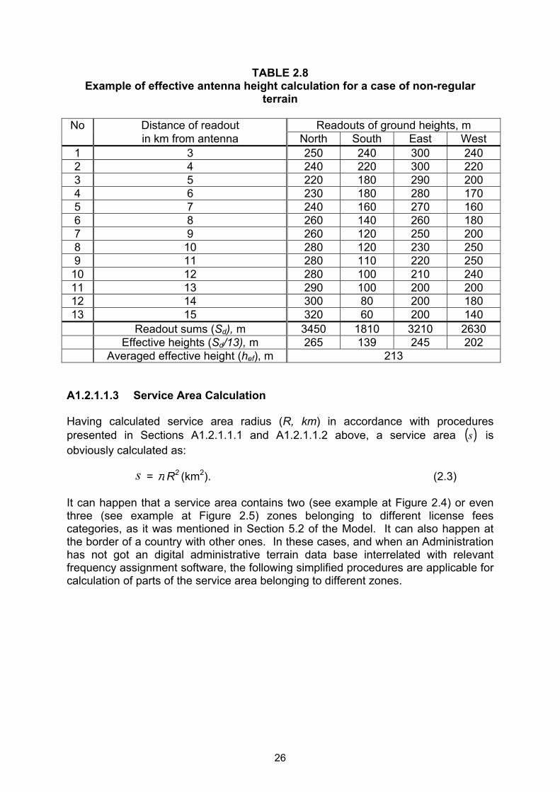
TABLE 2.8 Example of effective antenna height calculation for a case of non-regular
terrain No Distance of readout Readouts of ground heights, m
in km from antenna North South East West 1 3 250 240 300 240 2 4 240 220 300 220 3 5 220 180 290 200 4 6 230 180 280 170 5 7 240 160 270 160 6 8 260 140 260 180 7 9 260 120 250 200 8 10 280 120 230 250 9 11 280 110 220 250 10 12 280 100 210 240 11 13 290 100 200 200 12 14 300 80 200 180 13 15 320 60 200 140 Readout sums (Sd), m 3450 1810 3210 2630 Effective heights (Sd/13), m 265 139 245 202 Averaged effective height (hef), m 213
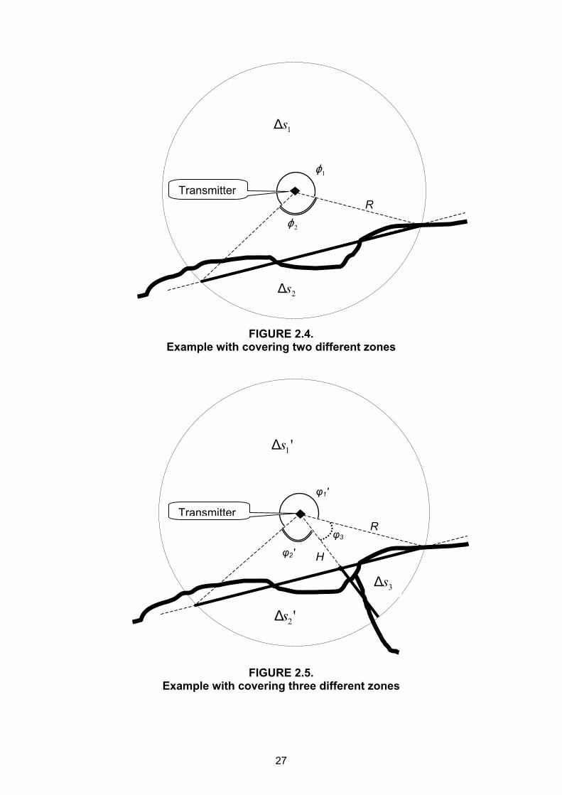
A1.2.1.1.3 Service Area Calculation Having calculated service area radius (R, km) in accordance with procedures presented in Sections A1.2.1.1.1 and A1.2.1.1.2 above, a service area is obviously calculated as:
( )s
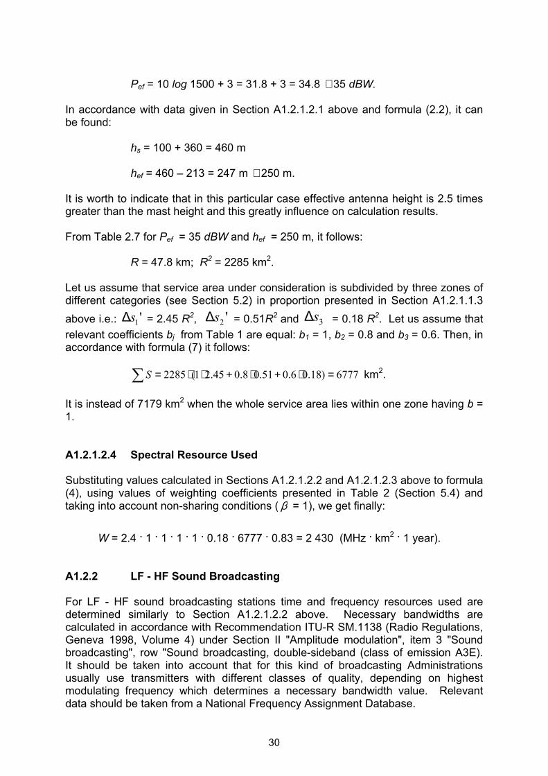
s = π R2 (km2). (2.3) It can happen that a service area contains two (see example at Figure 2.4) or even three (see example at Figure 2.5) zones belonging to different license fees categories, as it was mentioned in Section 5.2 of the Model. It can also happen at the border of a country with other ones. In these cases, and when an Administration has not got an digital administrative terrain data base interrelated with relevant frequency assignment software, the following simplified procedures are applicable for calculation of parts of the service area belonging to different zones.
26
1s∆
1ϕ
2ϕ
2s∆
R Transmitter
FIGURE 2.4. Example with covering two different zones
'1s∆
3s∆
'2s∆
φ1'
R Transmitter
H
φ3
φ2'
FIGURE 2.5. Example with covering three different zones
27
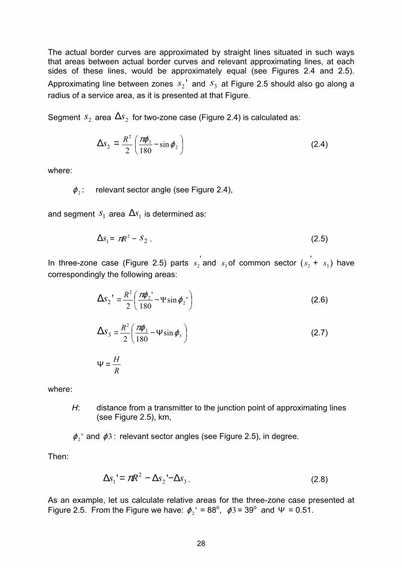
The actual border curves are approximated by straight lines situated in such ways that areas between actual border curves and relevant approximating lines, at each sides of these lines, would be approximately equal (see Figures 2.4 and 2.5). Approximating line between zones and at Figure 2.5 should also go along a radius of a service area, as it is presented at that Figure.
'2s 3s
Segment area for two-zone case (Figure 2.4) is calculated as: 2s 2s∆
=∆ 2s 2
2R
− 2
2 sin180
ϕπϕ (2.4)
where:
2ϕ : relevant sector angle (see Figure 2.4), and segment area is determined as: 1s 1s∆
= . (2.5) 1s∆ −2Rπ 2s In three-zone case (Figure 2.5) parts and of common sector ( + ) have correspondingly the following areas:
′2s 3s
′2s 3s
'2s∆
−= 'sinΨ
180'
2 22
2
ϕπϕR (2.6)
3s∆
Ψ−= 3
32
sin1802
ϕπϕR (2.7)
RH=Ψ
where:
H: distance from a transmitter to the junction point of approximating lines (see Figure 2.5), km,
'2ϕ and 3ϕ : relevant sector angles (see Figure 2.5), in degree.
Then: . (2.8) 32
21 '' ssRs ∆−∆−=∆ π
As an example, let us calculate relative areas for the three-zone case presented at Figure 2.5. From the Figure we have: '2ϕ = 88o, 3ϕ = 39o and = 0.51. Ψ
28

Then from (2.6), (2.7) and (2.8) it follows, correspondingly:
'2s∆
⋅−⋅= 999.051.0
18088
2
2 πR = 0.51R2
3s∆
⋅−⋅= 63.051.0
18039
2
2 πR = 0.18 R2
'1s∆ = (3.14 – 0.51 – 0.18) R2 = 2.45 R2.
A1.2.1.2 Example of Calculations A1.2.1.2.1 Incoming Parameters Let us calculate a spectral resource used by a FM sound broadcasting station working in an urban area 20 hours per each day with a power 1.5 kW in exclusive regime (no sharing). Antenna, having mast height 100 m, situated at the top of a hill with ground height 360 m above the sea level. Terrain situation around the transmitter corresponds to example presented in Section A1.2.1.1.2. above, i.e. average level of the ground between distances of 3 and 15 km from the transmitter (hav) in accordance with Table 2.8 equals to 213 m. Antenna gain against a half-wave dipole equals 3 dB. Modulation conditions are standard ones: peak deviation is 75 kHz, maximum modulation frequency is 15 kHz. A1.2.1.2.2 Time and Frequency Resources Used In accordance with formula (5), used time resource is: T = 20/24 (each day) = 0.83 year. According to Recommendation ITU-R SM.1138 (Radio Regulations, Geneva 1998, Volume 4) under Section III-A "Frequency modulation", item 3 "Sound broadcasting" (class of emission F3E) the necessary bandwidth is 180 kHz, i.e., accepting 1=χ , used frequency resource in accordance with formula (8) is: F = 0.18 MHz. A1.2.1.2.3 Territorial Resource Used Firstly, e.r.p. of the transmitter, effective antenna height and then service area radius should be calculated. In accordance with data presented in Section A1.2.1.2.1 above and formula (2.1), e.r.p. of the transmitter is:
29
Pef = 10 log 1500 + 3 = 31.8 + 3 = 34.8 35 dBW. ≅ In accordance with data given in Section A1.2.1.2.1 above and formula (2.2), it can be found: hs = 100 + 360 = 460 m hef = 460 – 213 = 247 m 250 m. ≅ It is worth to indicate that in this particular case effective antenna height is 2.5 times greater than the mast height and this greatly influence on calculation results. From Table 2.7 for Pef = 35 dBW and hef = 250 m, it follows: R = 47.8 km; R2 = 2285 km2. Let us assume that service area under consideration is subdivided by three zones of different categories (see Section 5.2) in proportion presented in Section A1.2.1.1.3 above i.e.: = 2.45 R'1s∆ 2, = 0.51R'2s∆ 2 and = 0.18 R3s∆ 2. Let us assume that relevant coefficients bj from Table 1 are equal: b1 = 1, b2 = 0.8 and b3 = 0.6. Then, in accordance with formula (7) it follows: km∑ =⋅+⋅+⋅⋅= 6777)18.06.051.08.045.21(2285S 2. It is instead of 7179 km2 when the whole service area lies within one zone having b = 1. A1.2.1.2.4 Spectral Resource Used Substituting values calculated in Sections A1.2.1.2.2 and A1.2.1.2.3 above to formula (4), using values of weighting coefficients presented in Table 2 (Section 5.4) and taking into account non-sharing conditions ( β = 1), we get finally: W = 2.4 . 1 . 1 . 1 . 1 . 0.18 . 6777 . 0.83 = 2 430 (MHz . km2 . 1 year). A1.2.2 LF - HF Sound Broadcasting For LF - HF sound broadcasting stations time and frequency resources used are determined similarly to Section A1.2.1.2.2 above. Necessary bandwidths are calculated in accordance with Recommendation ITU-R SM.1138 (Radio Regulations, Geneva 1998, Volume 4) under Section II "Amplitude modulation", item 3 "Sound broadcasting", row "Sound broadcasting, double-sideband (class of emission A3E). It should be taken into account that for this kind of broadcasting Administrations usually use transmitters with different classes of quality, depending on highest modulating frequency which determines a necessary bandwidth value. Relevant data should be taken from a National Frequency Assignment Database.
30
31
As far as it concerns a territorial resource used, its calculation for this case meets some difficulties due to complexity of calculations, especially for HF broadcasting, which hardly to be significantly simplified without loosing a minimal necessary accuracy. For MF transmitters service area greatly differ for day-time and night-time operations. Taking also into account that a number of LF – HF broadcasting stations in many countries is rather low, it is proposed instead of complicated calculations directly use relevant data on service area from a National Frequency Assignment Database. If those are not kept they can be asked from operators. Operators usually have information on their service areas through calculations and/or listening. On obtaining these data, related spectral resource used can be calculated similarly to the procedure presented in Section A1.2.1.2.3 above. . As far as for MF transmitters principally there are two considerable different values of service area for day-time and night-time operations, overall spectral resource used can be determined as a sum of two partial spectral resources which correspond to those different values of the service area. It should be also taken into account that service areas of LF, MF (night-time) and HF broadcasting transmitters can be very high ones and extend beyond borders of countries which sizes are not too high. In these cases (determined in co-operation with relevant operators) a service area can be considered by the territory of the whole country or its larger part. Areas of zones belonging to different categories (see Section 3.2) are determined by relevant administrative documentation or estimated by maps. In cases of directional transmitting antennas applications, a “service sector” concept, given by Recommendation ITU-R F.162-3, can be used (see details in Section A1.4.1 below).
A1.3 Mobile Radio Services A1.3.1 Land Mobile Radio Service A1.3.1.1 Background of Calculation Procedures The procedure follows radio wave propagation model known as modified Okamura-Hata one, the basis of which is given by Recommendation ITU-R P.529-2. The model assumes existence of homogeneous urban development in limits of the service area, lack of direct visibility between the transmitter of the base station and mobile personal receiver, heights of transmitting and receiving antennas are in limits 20 – 200 m (but in majority of cases they are 40 – 100 m) and 1.5 – 10 m correspondingly. Considering, for purposes of the given Model, that antenna feeder losses at transmitting and receiving sides are both equal zero, the power of a signal Pr (in dB above 1W) at an input of the receiver can be presented as:
Pr = Pt + Gt + Gr - L(R), dBW (3.1) where:
Pt: transmitter power, dBW
Gt: transmitter antenna gain, dB
Gr: receiver antenna gain, dB L(R): transmission losses between transmitter and receiver, dB. To provide the necessary quality of the received signal at a border of the service area the following condition should generally be met:
Pr = Pmin + kf σ where:
Pmin: minimal power of a received signal which equals to a sensitivity of the receiver, dBW
kf: fading allowance a signal for a given time of the signal quality
derogation
σ : mean square value of a signal fluctuations, dB. For 50% of time kf = 0, for 95% of time kf = 1.65. For conventional urban areas σ varies from 6 to 8 dB. Accepting, similarly to broadcasting, that a service area is
32
determined by the criterion of 50% time i.e. kf = 0, overall coefficient kf σ becomes equal zero and:
Pr = Pmin . (3.2) Equating right parts of formulas (3.1) and (3.2) to meet condition at the border of the service area, we get: Pt + Gt + Gr - L(R) = Pmin where: L(R) = Pt + Gt + Gr - Pmin . (3.3) In accordance with modified Okamura-Hata radio wave propagation model, accurate for a signal median value (i.e. for 50% of time):
L(R) = ξϑ + log R (3.4) where ϑ and ξ are coefficients in dB whose values depend on frequency and heights of a transmitter and receiver. For conventional urban areas: ξ = 44.9 – 6.55 log ht (3.5)
ϑ = 65.55 – 6.16 log f + 13.82 log ht + ar(hr) for f ≤ 1 GHz (3.6)
ϑ = 46.3 – 33.9 log f + 13.82 log ht + ar(hr) for f 1.5 GHz (3.7) ≥ where:
f: working frequency, MHz
ht: effective height of transmitting antenna, m hr: effective height of receiving antenna, m
ar(hr) = (1.1 log f – 0.7) hr - (1.56 log f – 0.8), dB. In accordance with Recommendation ITU-R P.529-2 effective height of transmitting antenna is to be determined as it presented in Recommendation ITU-R P.370-7 i.e. by procedure demonstrated in Sections A1.2.1.1.2 and A1.2.1.2.3. However, taking into account that recently powers of base stations are not to high and, therefore, related service areas are relatively small, for great majority of urban areas situated at a plain terrain, effective height of transmitting antenna can be approximated by its height above ground at a place of its installation. The antenna height of a mobile or portable station, in accordance with Recommendation ITU-R P.529-2, is taken as its height above the ground. These assumptions are taken for purposes of the given licence fees calculation Model.
33
Following formulas (3.3) - (3.7), a service area radius R can be calculated as:
−
= ξϑz
R 10 (3.8) where:
R: service area radius, km; z: easily determined generalised power parameter in dB, calculated as:
z = Pt + Gt + Gr - Pmin . (3.9)
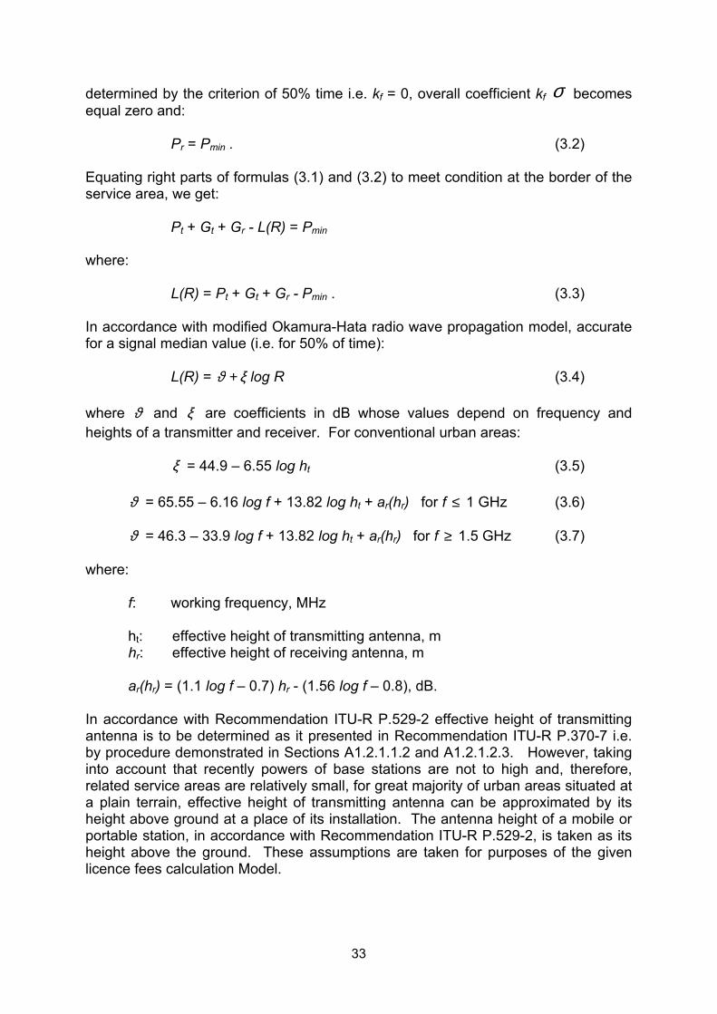
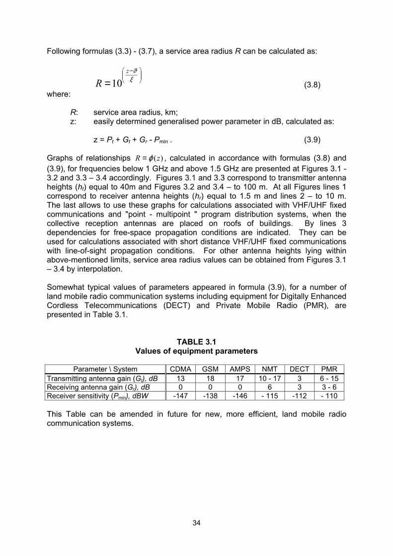
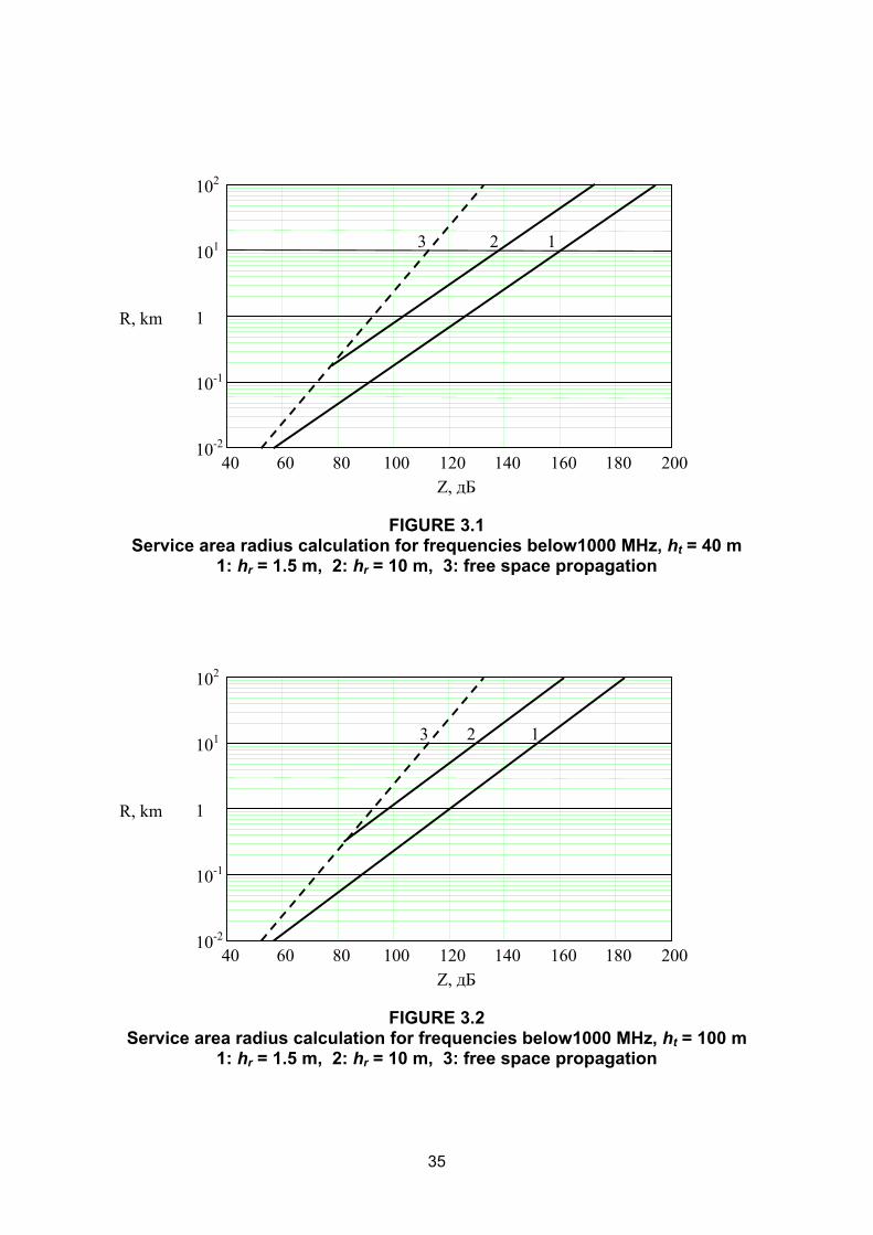
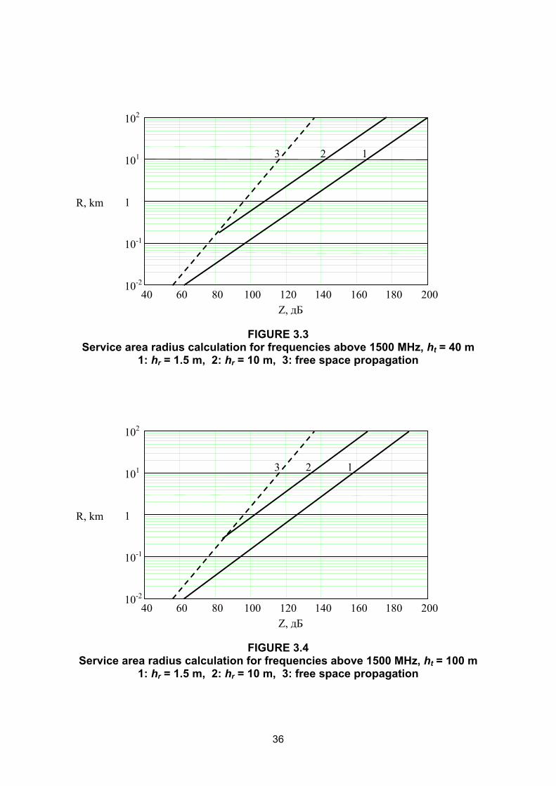
Graphs of relationships )(zR ϕ= , calculated in accordance with formulas (3.8) and (3.9), for frequencies below 1 GHz and above 1.5 GHz are presented at Figures 3.1 - 3.2 and 3.3 – 3.4 accordingly. Figures 3.1 and 3.3 correspond to transmitter antenna heights (ht) equal to 40m and Figures 3.2 and 3.4 – to 100 m. At all Figures lines 1 correspond to receiver antenna heights (hr) equal to 1.5 m and lines 2 – to 10 m. The last allows to use these graphs for calculations associated with VHF/UHF fixed communications and "point - multipoint " program distribution systems, when the collective reception antennas are placed on roofs of buildings. By lines 3 dependencies for free-space propagation conditions are indicated. They can be used for calculations associated with short distance VHF/UHF fixed communications with line-of-sight propagation conditions. For other antenna heights lying within above-mentioned limits, service area radius values can be obtained from Figures 3.1 – 3.4 by interpolation. Somewhat typical values of parameters appeared in formula (3.9), for a number of land mobile radio communication systems including equipment for Digitally Enhanced Cordless Telecommunications (DECT) and Private Mobile Radio (PMR), are presented in Table 3.1.
TABLE 3.1 Values of equipment parameters
Parameter \ System CDMA GSM AMPS NMT DECT PMR
Transmitting antenna gain (Gt), dB 13 18 17 10 - 17 3 6 - 15 Receiving antenna gain (Gr), dB 0 0 0 6 3 3 - 6 Receiver sensitivity (Pmin), dBW -147 -138 -146 - 115 -112 - 110 This Table can be amended in future for new, more efficient, land mobile radio communication systems.
34
Z, дБ40 60 80 100 120 140 160 180 200
10-2
10-1
1
101
102
R, km
123
FIGURE 3.1 Service area radius calculation for frequencies below1000 MHz, ht = 40 m
1: hr = 1.5 m, 2: hr = 10 m, 3: free space propagation
Z, дБ40 60 80 100 120 140 160 180 200
10-2
10-1
1
101
102
R, km
123
FIGURE 3.2 Service area radius calculation for frequencies below1000 MHz, ht = 100 m
1: hr = 1.5 m, 2: hr = 10 m, 3: free space propagation
35
Z, дБ40 60 80 100 120 140 160 180 200
10-2
10-1
1
101
102
R, km
123
FIGURE 3.3 Service area radius calculation for frequencies above 1500 MHz, ht = 40 m
1: hr = 1.5 m, 2: hr = 10 m, 3: free space propagation
Z, дБ40 60 80 100 120 140 160 180 200
10-2
10-1
1
101
102
R, km
123
FIGURE 3.4 Service area radius calculation for frequencies above 1500 MHz, ht = 100 m
1: hr = 1.5 m, 2: hr = 10 m, 3: free space propagation
36
A1.3.1.2 Calculation Procedures Having got graphs presented at Figures 3.1 - 3.4, calculation procedure becomes a quite simple one. It is only necessary to insert into formula (3.9) required parameters, taken from the National Frequency Assignment Database (or, in their absence, from Table 3.1), and to read related service area radius R for calculated value of parameter z directly from Figure 3.1 - 3.2, depending on working frequency and antenna heights. Due to the fact, that for land mobile service, and especially for cellular systems, service areas of individual base stations are rather small ones, they will usually lie within only one zone of license fees category. Thereby service areas usually can be calculated by simple formula (2.3). After determining service area value, procedure of used spectral resource calculation follows the same one, which is presented in Section A1.2.1.2. A1.3.1.3 Example of Calculations A1.3.1.3.1 Incoming Parameters Let us calculate a spectral resource used by a base station of GSM 900 MHz cellular system working with power 2.5 W without interruption 24 hours per each day, without sharing, in a city with population 40 000 inhabitants (i.e. according to Table 1 bj = 1.2). Overall frequency bands used for base – mobile and mobile – base transmissions are equal 0.8 MHz each. Transmitting and receiving antenna heights are 40 m and 1.5 m correspondently. Let us assume that other parameters correspond to Table 3.1. A1.3.1.3.2 Time and Frequency Resources Used In accordance with formula (5), used time resource is: T = 24/24 (each day) = 1.0 year. As far as the system within the same service area uses two sets of frequency bands, one for base – mobile and other for mobile – base transmissions, the overall used frequency resource, accepting in formula (8) 1=χ , can be found as:
F = 2 . 0.8 = 1.6 MHz. A1.3.1.3.3 Territorial Resource Used Substituting relevant data from Section A1.3.1.3.1 and Table 3.1 above to formula (3.9) we get:
z = 10 log 2.5 + 18+ 0 - (-138) = 160 dB.
37
For this z value from line 1 of Figure 3.1 and formula (2.3) it follows: R = 10 km, s = 314 km2. From formula (6), taking into account relevant data from Table 1, it follows: Si = 1.2 . 314 = 377 km2. A1.3.1.3.4 Spectral Resource Used Substituting values calculated in Sections A1.3.1.3.2 and A1.3.1.2.3 above to formula (4), using values of weighting coefficients presented in Table 2 (Section 5.4) and taking into account non-sharing conditions ( β = 1), we get finally:
W = 3 . 1.2 . 1 . 1 . 1 . 1.6 . 377 . 1 = 2 172 (MHz . km2 . 1 year). A1.3.2 Maritime Mobile Radio Service A1.3.2.1 Background of Calculation Procedures For coast and ship stations of Maritime Mobile Service working in VLF – HF frequency bands, proposed provisions for LF – HF broadcasting stations can be used (see Section A1.2.2 above) taking into account limitations by national maritime economical border (usually 200 miles, i.e. 360 km). In cases of directional transmitting antennas applications, a “service sector” concept, given by Recommendation ITU-R F.162-3, can be used (see details in Section A1.4.1 below). Service areas of VHF coast and ship stations working in 156 – 174 MHz frequency bands (Appendix S18 of the Radio Regulations), in accordance with provisions of Recommendation ITU-R P.616, are determined by propagation curves given in Annex 1 of Recommendation ITU-R P.370-7, i.e. on the same basis as for broadcasting (see Section A1.2.1 above). Technical characteristics of equipment are described in Recommendation ITU-R M.489-2. For ship stations having omnidirectional antennas service areas are calculated as:
( )s
s = π Rs
2 (km2) (3.10) where:
Rs radius of circular service area calculated from propagation curves of
Recommendation ITU-R P.370-7 for 30-250 MHz frequency band, sea, 50% of time and 50% of locations (Figure 1b of Recommendation ITU-R P.370-7).
38
It is necessary to note, that for this particular case the curves are the same for cold and warm seas. Transmitting antenna heights are actual antenna heights above the see level. For simplicity, receiving antenna heights for purposes of this particular calculation Model are accepted as to be equal 10 m in all cases. However it should be noted that in reality, to provide equal communication conditions between coast and ship stations in both directions, receiving antennas of coast stations are usually have the same heights than their transmitting antennas. Universal attenuation correction factor (Figure 8 of Recommendation ITU-R P.370-7), equals minus 5dB for all distances, is proposed to be applied. For coast stations it is accepted that one half of an occupied area, being a service one, with a radius Rs lies at a surface of see and the second half with a radius Rl - at a surface of land, i.e.: s = 0.5π (Rs
2 + Rl2) (km2) (3.11)
where;
Rl: radius of half-circular service area calculated from propagation curves of Recommendation ITU-R P.370-7 for 30-250 MHz frequency band, land, 50% of time and 50% of locations (Figure 1a of Recommendation ITU-R P.370-7, see Figure 2.1 above).
Effective antenna height calculations for land service area are provided similarly to broadcasting case (see Section A1.2.1.1.2 above). Similarly to broadcasting, for simplicity reason additional attenuation correction factor due to terrain irregularity is not applied. Taking into account that maritime mobile service belongs to safety services its reliability should be sufficiently high. Taking this into account, minimal usable field strength at the border of service area is accepted to be 30 dB above receiver reference sensitivity (2.0 µ V in accordance with Recommendation ITU-R M.489-2), i.e. Emu = 36 dB( µ V/m). Based on the above parameters and assumptions and accepting all antennas gains equal to 6 dB, relevant service/occupied areas radiuses were calculated for different transmitter powers from 10W to 50 W (maximal carrier power of coast stations in accordance with Recommendation ITU-R M.489-2) and various effective antenna heights presented in Recommendation ITU-R P.370-7. Results of calculations are presented in Table 3.2. Data for effective antenna heights 9,5 and 19 m were obtained by graphical approximation which is appropriate for purposes of this calculation Model. It is necessary to note that a land half-circle area of a coast station is only occupied but not service one because there are no ship stations there. Therefore its subdivision to different zones belonging to different license fees categories (like it is presented in section A1.2.1.1.3) can be eliminated and the only one category, corresponding to the largest occupied area, can be used. Moreover, an Administration may decide not to include this land half-circle area to territorial resource used. In this case radius Rl in formula (3.11) should be equal zero.
39
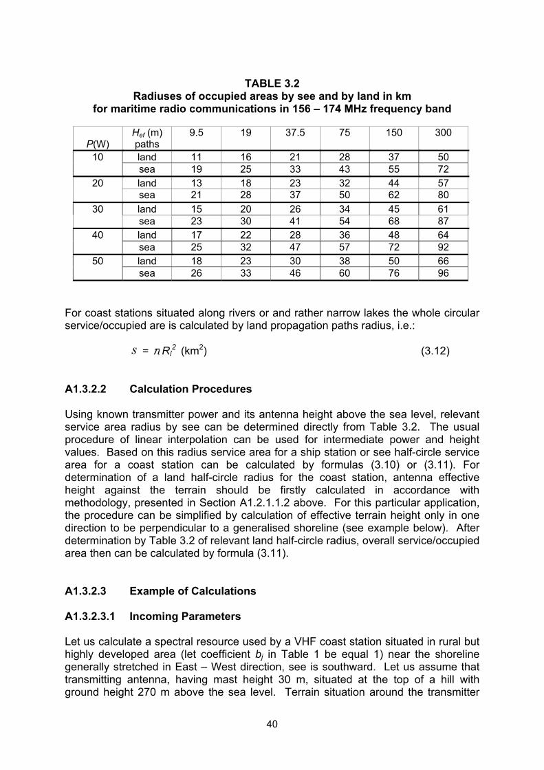
TABLE 3.2
Radiuses of occupied areas by see and by land in km for maritime radio communications in 156 – 174 MHz frequency band
P(W) Hef (m) paths
9.5 19 37.5 75 150 300
10 land 11 16 21 28 37 50 sea 19 25 33 43 55 72
20 land 13 18 23 32 44 57 sea 21 28 37 50 62 80
30 land 15 20 26 34 45 61 sea 23 30 41 54 68 87
40 land 17 22 28 36 48 64 sea 25 32 47 57 72 92
50 land 18 23 30 38 50 66 sea 26 33 46 60 76 96
For coast stations situated along rivers or and rather narrow lakes the whole circular service/occupied are is calculated by land propagation paths radius, i.e.:
s = π Rl2 (km2) (3.12)
A1.3.2.2 Calculation Procedures Using known transmitter power and its antenna height above the sea level, relevant service area radius by see can be determined directly from Table 3.2. The usual procedure of linear interpolation can be used for intermediate power and height values. Based on this radius service area for a ship station or see half-circle service area for a coast station can be calculated by formulas (3.10) or (3.11). For determination of a land half-circle radius for the coast station, antenna effective height against the terrain should be firstly calculated in accordance with methodology, presented in Section A1.2.1.1.2 above. For this particular application, the procedure can be simplified by calculation of effective terrain height only in one direction to be perpendicular to a generalised shoreline (see example below). After determination by Table 3.2 of relevant land half-circle radius, overall service/occupied area then can be calculated by formula (3.11). A1.3.2.3 Example of Calculations A1.3.2.3.1 Incoming Parameters Let us calculate a spectral resource used by a VHF coast station situated in rural but highly developed area (let coefficient bj in Table 1 be equal 1) near the shoreline generally stretched in East – West direction, see is southward. Let us assume that transmitting antenna, having mast height 30 m, situated at the top of a hill with ground height 270 m above the sea level. Terrain situation around the transmitter
40

corresponds to example presented in Section A1.2.1.1.2. above, i.e. effective height of the ground between distances of 3 and 15 km in the northern direction from the transmitter, calculated from column “North” of Table 2.8, equals to 265 m. In accordance with Section A1.3.2.2 for this application it represents average level of the ground (hav) in formula 2.2. Let us further assume that the transmitter power is 50 W and it works around the clock. Modulation conditions correspond to Recommendation ITU-R M. 489-2: class of emission F3E, deviation 5 kHz, necessary bandwidth 16 kHz. That also corresponds to Recommendation ITU-R SM.1138 (Radio Regulations, Geneva 1998, Volume 4) under Section III-A "Frequency modulation", item 2 "Telephony" (class of emission F3E).
±
A1.3.2.3.2 Time and Frequency Resources Used In accordance with formula (5), used time resource is: T = 24/24 (each day) = 1.0 year. Used frequency resource, accepting in formula (8) 1=χ , can be found as: F = 0.016 MHz. A1.3.2.3.3 Territorial Resource Used Following approach and data presented in Sections A1.3.2.1 and A1.3.2.3.1 effective antenna height for sea propagation paths equals to sum of antenna mast and site ground heights, i.e. (see also Section A1.2.1.1.2): hef = hs = 30 + 230 = 300 m. From Table 3.2 for transmitter with power 50 W and antenna height 300 m, sea propagation paths, it follows: Rs = 96 km. For land propagation paths in accordance with data of Section A1.3.2.3.1 and formula (2.2): hef = 300 m – 265 m = 35 m 37.5 m. ≈ From Table 3.2 for transmitter with power 50 W and antenna height 37.5 m, land propagation paths, it follows: Rl = 30 km.
41
Substituting calculated radiuses to formula (3.11) we get: s = 0.5π (962 + 302) = 15 890 km2 and, taking into account that bj = 1, from formula (6) it follows: S = s = 15 890 km2. A1.3.2.3.4 Spectral Resource Used Substituting values calculated in Sections A1.3.2.3.2 and A1.3.2.3.3 above to formula (4), using values of weighting coefficients presented in Table 2 (Section 5.4) and taking into account non-sharing conditions ( β = 1), we get finally:
W = 1 . 0.2 . 0.1 . 1 . 1 . 0.016 . 15 890 . 1 = 5.1 (MHz . km2 . 1 year). A1.3.3 Aeronautical Mobile, Radionavigation and Radiolocation Services A1.3.3.1 Calculation Procedures Common feature of these services is the fact that they provide radio communication (or location) operations with highly flying aircrafts. It leads to large service areas which borders are determined by distances up to radio horizon. If refraction of radio waves in the Earth’s atmosphere is taken into account,a distance up to a radio horizon (Rg) can be calculated by formula: Rg = 4.14 ( )rt hh + (km) (3.13). where:
ht: height of transmitting antenna above the averaged ground surface (at the ground or at the aircraft), m
hr: height of receiving antenna above the averaged ground surface (at the
ground or at the aircraft), m. With height of the aircraft 10 000 m and terrestrial antenna height 15 m, formula (3.12) gives radio horizon distance equals 429 km. Beyond the radio horizon the field strength sharply drops, as it is clearly demonstrated by curves of Recommendation ITU-R P.528. Therefore, in the given particular case, service area radius is accepted as to be equal to the distance up to the radio horizon irrespective to transmitter power and receiver sensitivity. The last parameters mainly determine only reliability of radio communication in the vicinity of service area borders in real influence environment that is very important for these of services as to be safety ones. Omnidirectional antennas are widely used. In cases of directional transmitting antennas applications (mainly in radionavigation and sectorial radiolocation), a
42
“service sector” concept, given by Recommendation ITU-R F.162-3, can be used (see details in Section A1.4.1 below). Taking into account that spectral resource used for these services, as to be safety ones) will not be too high, for simplicity reasons subdivision of the service area to different zones belonging to different license fees categories (like it is presented in section A1.2.1.1.3) can be eliminated and the only one category, corresponding to the largest occupied area, can be used. Given approach to the determination of service areas for aeronautical mobile, radionavigation and radiolocation services is proposed to be use for purposes of this calculation Model. The same approach can be accepted and for maritime radionavigation and radiolocation applications by using in formula (3.13) a target height equals about 10 m. A1.3.3.2 Examples of Calculations A1.3.3.2.1 Aeronautical Radio Communications A1.3.3.2.1.1 Incoming Parameters Let us calculate a spectral resource used by an aeronautical radiocommunication station working around the clock in 118 – 136 MHz band. Omnidirectional transmitting antenna height is 15 m and communications are provided with aircrafts flying at 10 000 m and higher, i.e in accordance with Section A1.3.3.1 Rg = 429 km. Let the largest occupied area lies in rural zone categorized by Table 1 as 0.8. Usual double-side AM is used (class of emission A3E), commercial quality. A1.3.3.2.1.2 Time and Frequency Resources Used In accordance with formula (5), used time resource is: T = 24/24 (each day) = 1.0 year. Following Recommendation ITU-R SM.1138 (Radio Regulations, Geneva 1998, Volume 4), Section II "Amplitude modulation", item 2 "Telephony", double-sideband (class of emission A3E), related necessary bandwidth is 6 kHz. Therefore, used frequency resource, accepting in formula (8) 1=χ , can be found as: F = 0.006 MHz. A1.3.3.2.1.3 Territorial Resource Used Substituting Rg = 429 km ito formula 2.3 we get: s = π . 4292 = 578 182 km2
43
and, taking into account that bj = 0.8, from formula (6) it follows: S = 0.8 . 578 182 = 462 546 km2. A1.3.3.2.1.4 Spectral Resource Used Substituting values calculated in Sections A1.3.3.3.1.2 and A1.3.3.3.1.3 above to formula (4), using values of weighting coefficients presented in Table 2 (Section 5.4) and taking into account non-sharing conditions ( β = 1), we get finally:
W = 0.1 . 0.2 . 0.1 . 0.8 . 1 . 0.006 . 462 546 . 1 = 4.4 (MHz . km2 . 1 year). A1.3.3.2.2 Primary Radars A1.3.3.2.2.1 Incoming Parameters Let us calculate a spectral resource used by an aeronautical primary radar working around the clock with circularly rotating antenna of 15 m height and set aside for locating aircrafts flying at 10 000 m and higher. It means that in accordance with Section A1.3.3.1 Rg = 429 km. Let the largest occupied area lies in rural zone categorized by Table 1 as 0.5. Radar uses shaped radio pulses with a half-amplitude duration equals 1 µ sec. A1.3.3.2.2.2 Time and Frequency Resources Used In accordance with formula (5), used time resource is: T = 24/24 (each day) = 1.0 year. Following Recommendation ITU-R SM.1138 (Radio Regulations, Geneva 1998, Volume 4), Section IV "Pulse modulation", item 1 "Radar", primary radar (class of emission P0N), related necessary bandwidth is 3 MHz. Therefore, used frequency resource, accepting in formula (8) 1.0=χ , can be found as: F = 0.1 . 3 = 0.3 MHz. A1.3.3.2.2.3 Territorial Resource Used Substituting Rg = 429 km to formula 2.3 we get: s = π . 4292 = 578 182 km2
44
and, taking into account that bj = 0.5, from formula (6) it follows: S = 0.5 . 578 182 = 289 091 km2. A1.3.3.2.2.4 Spectral Resource Used Substituting values calculated in Sections A1.3.3.3.2.2 and A1.3.3.3.2.3 above to formula (4), using values of weighting coefficients presented in Table 2 (Section 5.4) and taking into account non-sharing conditions ( β = 1), we get finally:
W = 0.1 . 0.02 . 0.1 . 0.2 . 1 . 0.3 . 289 091 . 1 = 3.5 (MHz . km2 . 1 year). A1.4 Fixed Radio Services A1.4.1 Calculation Procedures All fixed radio communications, HF radio links and UHF/SHF radio relay links (RRL), nowadays use directional and highly directional antennas. Taking this into account, for calculation of area occupied by an emission a "service sector" concept, given by Recommendation ITU-R F.162-3, can be used. This Recommendation states that for HF fixed links the service sector is very close to twice the angular width of the main beam measured to the half-power (- 3 dB) point. Taking into account the same physical background, for purposes of the given license fee calculation Model this concept is accepted for RRL links and for all other radio applications when directional antennas are used. Therefore, if relevant antenna beam-width is known (from the National Frequency Assignment Database or, on special request, from the operator or user) relevant emission occupied area can be determined as
so = 2
3602
cL⋅⋅πθ = 2
180 cL⋅⋅πθ (4.1)
where:
so: area occupied by an emission, km2
θ : antenna beam-width in degree
cL : length of the radio link, km. Fixed radio links, especially RRL, usually are planned very carefully, planning methods are sophisticated and significant fading allowances are usually used. Taking this into account and aiming to avoid complicated calculations, for purposes of the given Model it is proposed to use exact distance between relevant transmitter
45
and receiver as the length of the radio link . For RRL it will be one hop between two RRL stations.
cL
On determination of so , related territorial resource can be calculated in accordance with formula (6). Provisions concerning coverage of several zones belonging to different license fees categories are the same as in Section A1.2.1.1.3 although here influence of this factor is considerable smaller, especially for RRL, due to considerably smaller values of sector widths. Nevertheless, if an Administration likes to increase calculation accuracy, the following formula is applicable for the case when a service sector crosses two areas in approximately perpendicular direction at a distance Lb from the transmitter:
s1 = 2
180 bL⋅⋅πθ
s2 = )(180
22bc LL −⋅⋅πθ .
In accordance with the concept presented in Section A1.1, for overseas HF communications is determined by the distance from the transmitter to the country border in the direction of the transmission.
cL
Frequency and time resources and, then, spectral resource are calculated similarly to other cases above. As far as multi-station RRL can carry different numbers of channels at different hops due to branching and hop-lengths are different, spectral resources are calculated separately for each hop and then all values are summed. A1.4.2 Example of Calculations A1.4.2.1 Incoming Parameters Let us calculate a spectral resource used by one hop of a RRL in 2 GHz frequency band. Hop-length is 45 km, antenna beam-widths of both stations are 1.5o each (and it corresponds to G 40 dB). This hop lies within one zone categorised by Table 1 as 0.4 and carries 960 telephone channels in both directions with parameters corresponding those indicated in Recommendation ITU-R SM.1138 (Radio Regulations, Geneva 1998, Volume 4), Section III-A "Frequency modulation", subsection 5 "Composite emissions", RRL with 960 channels.
≈
A1.4.2.2 Time and Frequency Resources Used Taking into account principally continuous mode of RRL operation, from formula (5) it follows: T = 24/24 (each day) = 1.0 year.
46
In accordance with data, presented in above mentioned subsection of Recommendation ITU-R SM.1138 (Radio Regulations, Geneva 1998, Volume 4), Bn = 16.32 MHz (for both transmission directions). Therefore the overall used frequency resource, accepting in formula (8) 1=χ , can be found as:
F = 2 . 16.3 = 32.6 MHz. A1.4.2.3 Territorial Resource Used Substituting relevant data from Section A1.4.2.1 above to formula (4.1) we get: so = (1.5/180) . 3.14 . 452 = 53 km2. From formula (6), taking into account the zone category, it follows: S = 0.4 . 53 = 21 km2. A1.4.2.4 Spectral Resource Used Substituting values calculated in Sections A1.4.2.2 and A1.4.2.3 above to formula (4), using values of weighting coefficients presented in Table 2 (Section 5.4) and taking into account non-sharing conditions ( β = 1), we get finally: W = 0.1 . 0.1 . 1 . 0.2 . 1 . 32.6 . 21 . 1 = 1.4 (MHz . km2 . 1 year). A1.5 Earth Stations of Satellite Communications A1.5.1 Calculation Procedures Similarly to the case of fixed radio communication services presented in Section A1.4.1 above, for the calculation of occupied areas a "service sector" concept, given by Recommendation ITU-R F.162-3, is proposed to be used. As it was already indicated in Section A1.1 above, due to great difficulties in exact calculation of occupied areas of Earth stations of satellite communication systems, it is proposed to determine them on the basis of coordination distances agreed during the process of сoordination and notification of frequency and orbital assignments in the ITU-R. If these are not available an universal coordination distances of 350 km for VSAT-s and 750 km for other stations are proposed to be used. In some cases values agreed between Administration and operator can also be used. Occupied (necessary) bandwidth of an emission, or a bandwidth of a received signal, due to their absence in Recommendation ITU-R SM.1138, should be taken from related frequency assignment data, stored in a national Spectrum Management Database or received from an operator on a special request.
47
A1.5.2 Examples of Calculations
A1.5.2.1 Transmitting Earth Station A1.5.2.1.1 Incoming Parameters Let us calculate a spectral resource used by an earth station providing feeder link for non-GSO satellites operating in the Mobile-Satellite Service. Due to absence of more detailed data, coordination distance is accepted as to be 750 km. The station is situated in rural area and its antenna beam-widths is 0.5o. Occupied area of the emission lies within one zone categorized by Table 1 as 0.2. Let us assume that, in accordance with relevant frequency assignment recorded in the national Spectrum Management Database, the bandwidth of the emission is 200 MHz. A1.5.2.1.2 Time and Frequency Resources Used Taking into account principally continuous mode of feeder link operation, from formula (5) it follows: T = 24/24 (each day) = 1.0 year. In accordance with data presented in Section A1.5.2.1.1 above used frequency resource, accepting in formula (8) 1=χ , can be found as: F = 200 MHz. A1.5.2.1.3 Territorial Resource Used Substituting related data from Section A1.5.2.1.1 above to formula (4.1), where Lc represents coordination distance, we get: so = (0.5/180) . π . 7502 = 4 909 km2. From formula (6), taking into account the zone category, it follows: S = 0.2 . 4 909 = 982 km2. A1.5.2.1.4 Spectral Resource Used Substituting values calculated in Sections A1.5.2.1.2 and A1.5.2.1.3 above to formula (4), using values of weighting coefficients presented in Table 2 (Section 5.4) and taking into account non-sharing conditions ( β = 1), we get finally:
W = 1.4 . 0.1 . 0.1 . 0.2 . 1 . 200 . 982 . 1 = 550 (MHz . km2 . 1 year).
48
A1.5.2.2 Receiving Earth Station A1.5.2.2.1 Incoming Parameters Let us calculate a spectral resource used by a receiving VSAT earth station working around the clock. Due to absence more detailed data, coordination distance is taken as 350 km. The station is situated in rural area and its antenna beam-widths is 1o. Occupied area of the emission lies within one zone categorised by Table 1 as 0.3. Let us assume that, in accordance with relevant frequency assignment recorded in the national Spectrum Management Database, the bandwidth of the received signal is 30 MHz. A1.5.2.2.2 Time and Frequency Resources Used Assuming continuous mode of the station operation, from formula (5) it follows: T = 24/24 (each day) = 1.0 year. In accordance with data presented in Section A1.5.2.2.1 above used frequency resource, accepting in formula (8) 1=χ , can be found as: F = 30 MHz. A1.5.2.2.3 Territorial Resource Used Substituting related data from Section A1.5.2.2.1 above to formula (4.1), where Lc represents coordination distance, we get: so = (1/180) . π . 3502 = 2 138 km2. From formula (6), taking into account the zone category, it follows: S = 0.3 . 2 138 = 641 km2. A1.5.2.2.4 Spectral Resource Used Substituting values calculated in Sections A1.5.2.1.2 and A1.5.2.1.3 above to formula (4), using values of weighting coefficients presented in Table 2 (Section 5.4) and taking into account non-sharing conditions ( β = 1), we get finally:
W = 1.4 . 0.1 . 0.1 . 0.2 . 1 . 30 . 641 . 1 = 54 (MHz . km2 . 1 year).
49
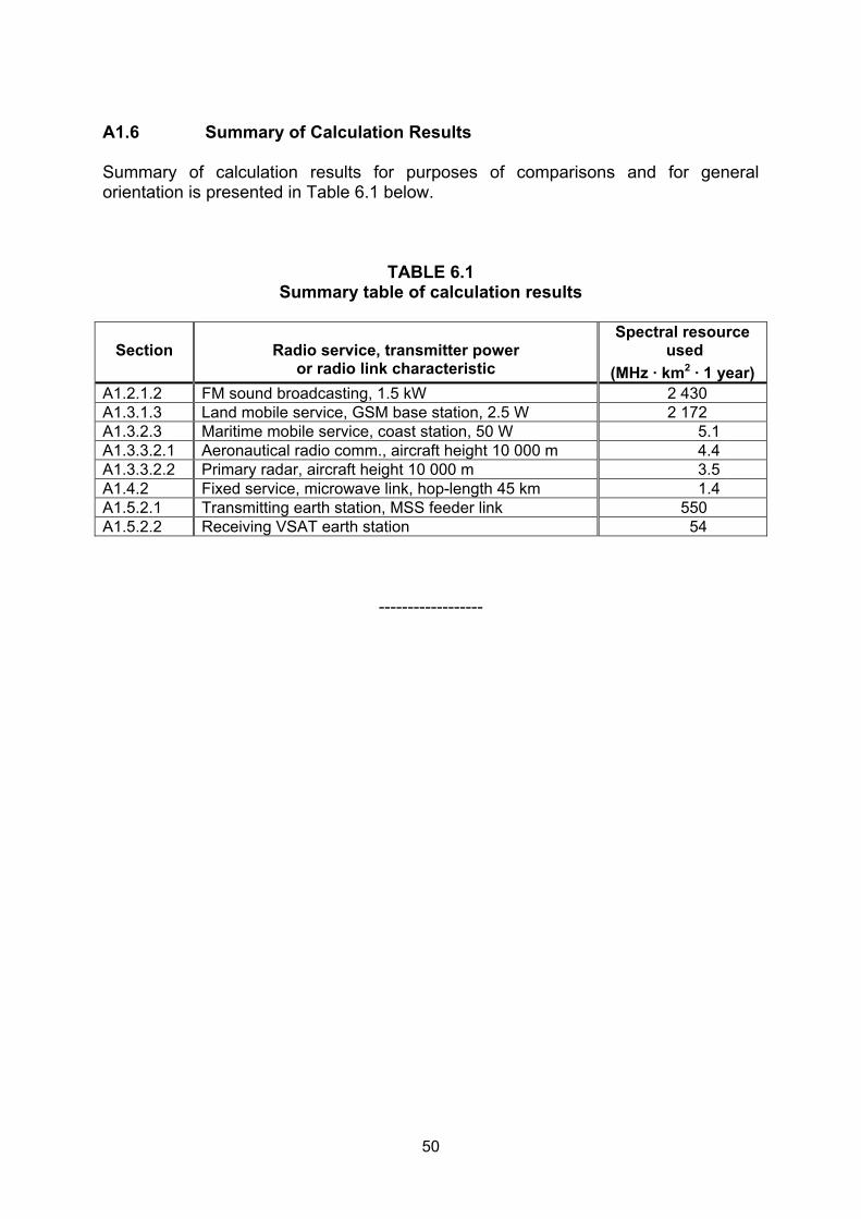
50
A1.6 Summary of Calculation Results Summary of calculation results for purposes of comparisons and for general orientation is presented in Table 6.1 below.
TABLE 6.1 Summary table of calculation results
Section
Radio service, transmitter power or radio link characteristic
Spectral resource used
(MHz . km2 . 1 year) A1.2.1.2 FM sound broadcasting, 1.5 kW 2 430 A1.3.1.3 Land mobile service, GSM base station, 2.5 W 2 172 A1.3.2.3 Maritime mobile service, coast station, 50 W 5.1 A1.3.3.2.1 Aeronautical radio comm., aircraft height 10 000 m 4.4 A1.3.3.2.2 Primary radar, aircraft height 10 000 m 3.5 A1.4.2 Fixed service, microwave link, hop-length 45 km 1.4 A1.5.2.1 Transmitting earth station, MSS feeder link 550 A1.5.2.2 Receiving VSAT earth station 54
------------------