Part II - Galois Theory - dec41.user.srcf.netdec41.user.srcf.net/notes/II_M/galois_theory.pdf ·...
71
Part II — Galois Theory Based on lectures by C. Birkar Notes taken by Dexter Chua Michaelmas 2015 These notes are not endorsed by the lecturers, and I have modified them (often significantly) after lectures. They are nowhere near accurate representations of what was actually lectured, and in particular, all errors are almost surely mine. Groups, Rings and Modules is essential Field extensions, tower law, algebraic extensions; irreducible polynomials and relation with simple algebraic extensions. Finite multiplicative subgroups of a field are cyclic. Existence and uniqueness of splitting fields. [6] Existence and uniqueness of algebraic closure. [1] Separability. Theorem of primitive element. Trace and norm. [3] Normal and Galois extensions, automorphic groups. Fundamental theorem of Galois theory. [3] Galois theory of finite fields. Reduction mod p. [2] Cyclotomic polynomials, Kummer theory, cyclic extensions. Symmetric functions. Galois theory of cubics and quartics. [4] Solubility by radicals. Insolubility of general quintic equations and other classical problems. [3] Artin’s theorem on the subfield fixed by a finite group of automorphisms. Polynomial invariants of a finite group; examples. [2] 1
-
Upload
duongquynh -
Category
Documents
-
view
213 -
download
0
Transcript of Part II - Galois Theory - dec41.user.srcf.netdec41.user.srcf.net/notes/II_M/galois_theory.pdf ·...

Part II — Galois Theory
Based on lectures by C. BirkarNotes taken by Dexter Chua
Michaelmas 2015
These notes are not endorsed by the lecturers, and I have modified them (oftensignificantly) after lectures. They are nowhere near accurate representations of what
was actually lectured, and in particular, all errors are almost surely mine.
Groups, Rings and Modules is essential
Field extensions, tower law, algebraic extensions; irreducible polynomials and relationwith simple algebraic extensions. Finite multiplicative subgroups of a field are cyclic.Existence and uniqueness of splitting fields. [6]
Existence and uniqueness of algebraic closure. [1]
Separability. Theorem of primitive element. Trace and norm. [3]
Normal and Galois extensions, automorphic groups. Fundamental theorem of Galoistheory. [3]
Galois theory of finite fields. Reduction mod p. [2]
Cyclotomic polynomials, Kummer theory, cyclic extensions. Symmetric functions.Galois theory of cubics and quartics. [4]
Solubility by radicals. Insolubility of general quintic equations and other classicalproblems. [3]
Artin’s theorem on the subfield fixed by a finite group of automorphisms. Polynomial
invariants of a finite group; examples. [2]
1
Contents II Galois Theory
Contents
0 Introduction 3
1 Solving equations 4
2 Field extensions 72.1 Field extensions . . . . . . . . . . . . . . . . . . . . . . . . . . . . 72.2 Ruler and compass constructions . . . . . . . . . . . . . . . . . . 122.3 K-homomorphisms and the Galois Group . . . . . . . . . . . . . 142.4 Splitting fields . . . . . . . . . . . . . . . . . . . . . . . . . . . . 162.5 Algebraic closures . . . . . . . . . . . . . . . . . . . . . . . . . . 192.6 Separable extensions . . . . . . . . . . . . . . . . . . . . . . . . . 222.7 Normal extensions . . . . . . . . . . . . . . . . . . . . . . . . . . 302.8 The fundamental theorem of Galois theory . . . . . . . . . . . . . 332.9 Finite fields . . . . . . . . . . . . . . . . . . . . . . . . . . . . . . 36
3 Solutions to polynomial equations 403.1 Cyclotomic extensions . . . . . . . . . . . . . . . . . . . . . . . . 403.2 Kummer extensions . . . . . . . . . . . . . . . . . . . . . . . . . 443.3 Radical extensions . . . . . . . . . . . . . . . . . . . . . . . . . . 473.4 Solubility of groups, extensions and polynomials . . . . . . . . . 503.5 Insolubility of general equations of degree 5 or more . . . . . . . 54
4 Computational techniques 594.1 Reduction mod p . . . . . . . . . . . . . . . . . . . . . . . . . . . 594.2 Trace, norm and discriminant . . . . . . . . . . . . . . . . . . . . 62
2
0 Introduction II Galois Theory
0 Introduction
The most famous result of Galois theory is that there is no general solution topolynomial equations of degree 5 or above in terms of radicals. However, thisresult was, in fact, proven before Galois theory existed, and goes under the nameof the Abel–Ruffini theorem. What Galois theory does provides is a way to decidewhether a given polynomial has a solution in terms of radicals, as well as a niceway to prove this result.
However, Galois theory is more than equation solving. In fact, the funda-mental theorem of Galois theory, which is obviously an important theorem inGalois theory, has completely nothing to do with equation solving. Instead, it isabout group theory.
In modern days, Galois theory is often said to be the study of field extensions.The idea is that we have a field K, and then add more elements to get a field L.When we want to study solutions to polynomial equations, what we add is theroots of the polynomials. We then study the properties of this field extension,and in some cases, show that this field extension cannot be obtained by justadding radicals.
For certain “nice” field extensions K ⊆ L, we can assign to it the Galois groupGal(L/K). In general, given any group G, we can find subgroups of G. On theother hand, given a field extension K ⊆ L, we can try to find some intermediatefield F that can be fitted into K ⊆ F ⊆ L. The key idea of Galois theory isthat these two processes are closely related — we can establish a one-to-onecorrespondence between the subgroups of G and the intermediate fields F .
Moreover, many properties of (intermediate) field extensions correspond toanalogous ideas in group theory. For example, we have the notion of normalsubgroups, and hence there is an analogous notion of normal extensions. Similarly,we have soluble extensions (i.e. extensions that can be obtained by addingradicals), and these correspond to “soluble groups”. In Galois theory, we willstudy how group-theoretic notions and field-theoretic notions interact.
Nowadays, Galois theory is an important field in mathematics, and finds itsapplications in number theory, algebraic geometry and even cryptography.
3
1 Solving equations II Galois Theory
1 Solving equations
Galois theory grew of of the desire to solve equations. In particular, to solvepolynomial equations. To begin with, we will come up with general solutions topolynomial equations of up to degree 4. However, this is the best we can do, aswe will later show in the course — there is no general solution to polynomialequations of degree 5 or above.
Before we start, we will define some notations that we will frequently use.If R is a ring, then R[t] is the polynomial ring over R in the variable t.
Usually, we take R = Q and consider polynomials f(t) ∈ Q[t]. The objectiveis then to find roots to the equation f(t) = 0. Often, we want to restrict oursearch domain. For example, we might ask if there is a root in Q. We will thususe Rootf (X) to denote the set of all roots of f in X.
Linear equations
Suppose that f = t+ a ∈ Q[t] (with a ∈ Q). This is easy to solve — we haveRootf (Q) = {−a}.
Quadratic equations
Consider a simple quadratic f = t2 + 1 ∈ Q[t]. Then Rootf (Q) = ∅ since thesquare of all rationals are positive. However, in the complex plane, we haveRootf (C) = {
√−1,−
√−1}.
In general, let f = t2 + at + b ∈ Q[t]. Then as we all know, the roots aregiven by
Rootf (C) =
{−a±
√a2 − 4b
2
}
Cubic equations
Let f = t3 + c ∈ Q[t]. The roots are then
Rootf (C) = { 3√−c, µ 3
√−c, µ2 3
√−c},
where µ = −1+√−3
2 is the 3rd root of unity. Note that µ is defined by theequation µ3 − 1 = 0, and satisfies µ2 + µ+ 1 = 0.
In general, let f = t3 + at2 + bt+ c ∈ Q[t], and let Rootf (C) = {α1, α2, α3},not necessarily distinct.
Our objective is to solve f = 0. Before doing so, we have to make it explicitwhat we mean by “solving” the equation. As in solving the quadratic, we wantto express the roots α1, α2 and α3 in terms of “radicals” involving a, b and c.
Unlike the quadratic case, there is no straightforward means of coming upwith a general formula. The result we currently have is the result of manymany years of hard work, and the substitutions we make seemingly come out ofnowhere. However, after a lot of magic, we will indeed come up with a generalformula for it.
We first simplify our polynomial by assuming a = 0. Given any polynomialf = t3 + at2 + bt+ c, we know a is the negative of the sum of the roots. So wecan increase each root by a
3 so that the coefficient of t2 vanishes. So we perform
4
1 Solving equations II Galois Theory
the change of variables t 7→ t− a3 , and get rid of the coefficient of t2. So we can
assume a = 0.Let µ be as above. Define
β = α1 + µα2 + µ2α3
γ = α1 + µ2α2 + µα3
These are the Lagrange resolvers. We obtain
βγ = α21 + α2
2 + α23 + (µ+ µ2)(α1α2 + α2α3 + α1α3)
Since µ2 + µ+ 1 = 0, we have µ2 + µ = −1. So we can simplify to obtain
= (α1 + α2 + α3)2 − 3(α1α2 + α2α3 + α1α3)
We have α1 + α2 + α3 = −a = 0, while b = α1α2 + α2α3 + α1α3. So
= −3b
Cubing, we obtain
β3γ3 = −27b3.
On the other hand, recalling again that α1 + α2 + α3 = 0, we have
β3 + γ3 = (α1 + µα2 + µ2α3)3 + (α1 + µ2α2 + µα3)3 + (α1 + α2 + α3)3
= 3(α21 + α3
2 + α23) + 18α1α2α3
We have α1α2α3 = −c, and since α3i + bαi + c = 0 for all i, summing gives
α31 + α3
2 + α33 + 3c = 0. So
= −27c
Hence, we obtain(t− β3)(t− γ3) = t2 + 27ct− 27b3.
We already know how to solve this equation using the quadratic formula. Weobtain
{β3, γ3} =
{−27c±
√(27c)2 + 4× 27b3
2
}We now have β3 and γ3 in terms of radicals. So we can find β and γ in terms ofradicals. Finally, we can solve for αi using
0 = α1 + α2 + α3
β = α1 + µα2 + µ2α3
γ = α1 + µ2α2 + µα3
In particular, we obtain
α1 =1
3(β + γ)
α2 =1
3(µ2β + µγ)
α3 =1
3(µβ + µ2γ)
5
1 Solving equations II Galois Theory
So we can solve a cubic in terms of radicals.This was a lot of magic involved, and indeed this was discovered through a
lot of hard work throughout many many years. This is also not a very helpfulresult since we have no idea where these substitutions came from and why theyintuitively work.
Quartic equations
Assume f = t4 + at3 + bt2 + ct + d ∈ Q[t]. Let Rootf (C) = {α1, α2, α3, α4}.Can we express all these in terms of radicals? Again the answer is yes, but theprocedure is much more complicated.
We can perform a similar change of variable to assume a = 0. So α1 + α2 +α3 + α4 = 0.
This time, define
β = α1 + α2
γ = α1 + α3
λ = α1 + α4
Doing some calculations, we see that
β2 = −(α1 + α2)(α3 + α4)
γ2 = −(α1 + α3)(α2 + α4)
λ2 = −(α1 + α4)(α2 + α3)
Now consider
g = (t− β2)(t− γ2)(t− λ2)
= t3 + 2bt2 + (b2 − 4d)t− c2
This we know how to solve, and so we are done.
Quintics and above
So far so good. But how about polynomials of higher degrees? In general, letf ∈ Q[t]. Can we write down all the roots of f in terms of radicals? We knowthat the answer is yes if deg f ≤ 4.
Unfortunately, for deg f ≥ 5, the answer is no. Of course, this “no” meansno in general. For example, f = (t− 1)(t− 2) · · · (t− 5) ∈ Q[t] has the obviousroots in terms of radicals.
There isn’t an easy proof of this result. The general idea is to first associatea field extension F ⊇ Q for our polynomial f . This field F will be obtainedby adding all roots of f . Then we associate a Galois group G to this fieldextension. We will then prove a theorem that says f has a solution in termsof radicals if and only if the Galois group is “soluble”, where “soluble” has aspecific algebraic definition in group theory we will explore later. Finally, wefind specific polynomials whose Galois group is not soluble.
6
2 Field extensions II Galois Theory
2 Field extensions
After all that (hopefully) fun introduction and motivation, we will now startGalois theory in a more abstract way. The modern approach is to describe thesein terms of field extensions.
2.1 Field extensions
Definition (Field extension). A field extension is an inclusion of a field K ⊆ L,where K inherits the algebraic operations from L. We also write this as L/K.Alternatively, we can define this by a injective homomorphism K → L. We sayL is an extension of K, and K is a subfield of L.
Example.
(i) R/Q is a field extension.
(ii) C/Q is a field extension.
(iii) Q(√
2) = {a+ b√
2 : a, b ∈ Q} ⊆ R is a field extension over Q.
Given a field extension L/K, we want to quantify how much “bigger” Lis compared to K. For example, to get from Q to R, we need to add a lot ofelements (since Q is countable and R is uncountable). On the other hand, to getfrom R to C, we just need to add a single element
√−1.
To do so, we can consider L as a vector space over K. We know that Lalready comes with an additive abelian group structure, and we can define scalarmultiplication by simply multiplying: if a ∈ K,α ∈ L, then a · α is defined asmultiplication in L.
Definition (Degree of field extension). The degree of L over K is [L : K] is thedimension of L as a vector space over K. The extension is finite if the degree isfinite.
In this course, we are mostly concerned with finite extensions.
Example.
(i) Consider C/R. This is a finite extension with degree [C : R] = 2 since wehave a basis of {1, i}.
(ii) The extension Q(√
2)/Q has degree 2 since we have a basis of {1,√
2}.
(iii) The extension R/Q is not finite.
We are going to use the following result a lot:
Theorem (Tower Law). Let F/L/K be field extensions. Then
[F : K] = [F : L][L : K]
Proof. Assume [F : L] and [L : K] are finite. Let {α1, · · · , αm} be a basis forL over K, and {β1, · · · , βn} be a basis for F over L. Pick γ ∈ F . Then we canwrite
γ =∑i
biβi, bi ∈ L.
7

2 Field extensions II Galois Theory
For each bi, we can write as
bi =∑j
aijαj , aij ∈ K.
So we can write
γ =∑i
∑j
aijαj
βi =∑i,j
aijαjβi.
So T = {αjβi}i,j spans F over K. To show that this is a basis, we have to showthat they are linearly independent. Consider the case where γ = 0. Then wemust have bi = 0 since {βi} is a basis of F over L. Hence each aij = 0 since{αj} is a basis of L over K.
This implies that T is a basis of F over K. So
[F : K] = |T | = nm = [F : L][L : K].
Finally, if [F : L] = ∞ or [L : K] = ∞, then clearly [F : K] = ∞ as well. Soequality holds as well.
Recall that in IA Numbers and Sets, we defined a real number x to bealgebraic if it is a root of some polynomial in integer (or rational) coefficients.We can do this for general field (extensions) as well.
Definition (Algebraic number). Let L/K be a field extension, α ∈ L. Wedefine
Iα = {f ∈ K[t] : f(α) = 0} ⊆ K[t]
This is the set of polynomials for which α is a root. It is easy to show that Iα isan ideal, since it is the kernel of the ring homomorphism K[t]→ L by g 7→ g(α).
We say α is algebraic over K if Iα 6= 0. Otherwise, α is transcendental overK.
We say L is algebraic over K if every element of L is algebraic.
Example.
(i) 9√
7 is algebraic over Q because f( 9√
7) = 0, where f = t9 − 7. In general,any number written with radicals is algebraic over Q.
(ii) π is not algebraic over Q.
These are rather simple examples, and the following lemma will provide us away of generating much more examples.
Lemma. Let L/K be a finite extension. Then L is algebraic over K.
Proof. Let n = [L : K], and let α ∈ L. Then 1, α, α2, · · · , αn are linearlydependent over K (since there are n+ 1 elements). So there exists some ai ∈ K(not all zero) such that
anαn + an−1α
n−1 + · · ·+ a1α+ a0 = 0.
So we have a non-trivial polynomial that vanishes at α. So α is algebraic overK.
Since α was arbitrary, L itself is algebraic.
8
2 Field extensions II Galois Theory
If L/K is a field extension and α ∈ L is algebraic, then by definition, there issome polynomial f such that f(α) = 0. It is a natural question to ask if there isa “smallest” polynomial that does this job. Obviously we can find a polynomialof smallest degree (by the well-ordering principle of the natural numbers), butwe can get something even stronger.
Since K is a field, K[t] is a PID (principal ideal domain). This, by definition,implies we can find some (monic) Pα ∈ K[t] such that Iα = 〈Pα〉. In other words,every element of Iα is just a multiple of Pα.
Definition (Minimal polynomial). Let L/K be a field extension, α ∈ L. Theminimal polynomial of α over K is a monic polynomial Pα such that Iα = 〈Pα〉.
Example.
(i) Consider R/Q, α = 3√
2. Then the minimal polynomial is Pα = t3 − 2.
(ii) Consider C/R, α = 3√
2. Then the minimal polynomial is Pα = t− 3√
2.
It should be intuitively obvious that by virtue of being “minimal”, theminimal polynomial is irreducible.
Proposition. Let L/K be a field extension, α ∈ L algebraic over K, and Pαthe minimal polynomial. Then Pα is irreducible in K[t].
Proof. Assume that Pα = QR in K[t]. So 0 = Pα(α) = Q(α)R(α). So Q(α) = 0or R(α) = 0. Say Q(α) = 0. So Q ∈ Iα. So Q is a multiple of Pα. However, wealso know that Pα is a multiple of Qα. This is possible only if R is a unit inK[t], i.e. R ∈ K. So Pα is irreducible.
It should also be clear that if f is irreducible and f(α) = 0, then f is theminimal polynomial. Often, it is the irreducibility of Pα that is important.
Apart from the minimal polynomial, we can also ask for the minimal fieldcontaining α.
Definition (Field generated by α). Let L/K be a field extension, α ∈ L. Wedefine K(α) to be the smallest subfield of L containing K and α. We call K(α)the field generated by α over K.
This definition by itself is rather abstract and not very helpful. Intuitively,K(α) is what we get when we add α to K, plus all the extra elements needed tomake K(α) a field (i.e. closed under addition, multiplication and inverse). Wecan express this idea more formally by the following result:
Theorem. Let L/K a field extension, α ∈ L algebraic. Then
(i) K(α) is the image of the (ring) homomorphism φ : K[t]→ L defined byf 7→ f(α).
(ii) [K(α) : K] = degPα, where Pα is the minimal polynomial of α over K.
Note that the kernel of the homomorphism φ is (almost) by definition theideal 〈Pα〉. So this theorem tells us
K[t]
〈Pα〉∼= K(α).
9
2 Field extensions II Galois Theory
Proof.
(i) Let F be the image of φ. The first step is to show that F is indeed a field.Since F is the image of a ring homomorphism, we know F is a subring ofL. Given β ∈ F non-zero, we have to find an inverse.
By definition, β = f(α) for some f ∈ K[t]. The idea is to use Bezout’sidentity. Since β 6= 0, f(α) 6= 0. So f 6∈ Iα = 〈Pα〉. So Pα - f in K[t]. SincePα is irreducible, Pα and f are coprime. Then there exists some g, h ∈ K[t]such that fg + hPα = 1. So f(α)g(α) = f(α)g(α) + h(α)Pα(α) = 1. Soβg(α) = 1. So β has an inverse. So F is a field.
From the definition of F , we have K ⊆ F and α ∈ F , using the constantpolynomials f = c ∈ K and the identity f = t.
Now, if K ⊆ G ⊆ L and α ∈ G, then G contains all the polynomialexpressions of α. Hence F ⊆ G. So K(α) = F .
(ii) Let n = degPα. We show that {1, α, α2, · · · , αn−1} is a basis for K(α)over K.
First note that since degPα = n, we can write
αn =
n−1∑i=0
aiαi.
So any other higher powers are also linear combinations of the αis (byinduction). This means that K(α) is spanned by 1, · · · , αn−1 as a K vectorspace.
It remains to show that {1, · · · , αn−1} is linearly independent. Assumenot. Then for some bi, we have
n−1∑i=0
biαi = 0.
Let f =∑bit
i. Then f(α) = 0. So f ∈ Iα = 〈Pα〉. However, deg f <degPα. So we must have f = 0. So all bi = 0. So {1, · · · , αn−1} is a basisfor K(α) over K. So [K(α) : K] = n.
Corollary. Let L/K be a field extension, α ∈ L. Then α is algebraic over K ifand only if K(α)/K is a finite extension.
Proof. If α is algebraic, then [K(α) : K] = degPα < ∞ by above. So theextension is finite.
If K ⊆ K(α) is a finite extension, then by previous lemma, the entire K(α)is algebraic over K. So α is algebraic over K.
We can extend this definition to allow more elements in the generating set.
Definition (Field generated by elements). Let L/K be a field extension,α1, · · · , αn ⊆ L. We define K(α1, · · · , αn) to be the smallest subfield of Lcontaining K and α1, · · · , αn.
We call K(α1, · · · , αn) the field generated by α1, · · · , αn over K.
And we can prove some similar results.
10

2 Field extensions II Galois Theory
Theorem. Suppose that L/K is a field extension.
(i) If α1, · · · , αn ∈ L are algebraic over K, then K(α1, · · · , αn)/K is a finiteextension.
(ii) If we have field extensions L/F/K and F/K is a finite extension, thenF = K(α1, · · · , αn) for some α1, · · · , αn ∈ L.
Proof.
(i) We prove this by induction. Since α1 is algebraic over K, K ⊆ K(α1) is afinite extension.
For 1 ≤ i < n, αi+1 is algebraic over K. So αi+1 is also algebraicover K(α1, · · · , αi). So K(α1, · · · , αi) ⊆ K(α1, · · · , αi)(αi+1) is a finiteextension. But K(α1, · · · , αi)(αi+1) = K(α1, · · · , αi+1). By the tower law,K ⊆ K(αi, · · · , αi+1) is a finite extension.
(ii) Since F is a finite dimensional vector space over K, we can take a basis{α1, · · · , αn} of F over K. Then it should be clear that F = K(α1, · · · , αn).
When studying polynomials, the following result from IB Groups, Rings andModules is often helpful:
Proposition (Eisenstein’s criterion). Let f = antn + · · · + a1t + a0 ∈ Z[t].
Assume that there is some prime number p such that
(i) p | ai for all i < n.
(ii) p - an
(iii) p2 - a0.
Then f is irreducible in Q[t].
Example. Consider the field extensions
Q ⊆ Q(√
2) ⊆ Q(√
2,3√
2) ⊆ R,
Q ⊆ Q(3√
2) ⊆ Q(√
2,3√
2) ⊆ R.
We have [Q(√
2) : Q] = 2 since {1,√
2} is a basis of Q(√
2) over Q.How about [Q( 3
√2) : Q]? By the Eisenstein criterion, we know that t3 − 2 is
irreducible in Q[t]. So the minimal polynomial of 3√
2 over Q is t3 − 2 which hasdegree 3. So [Q( 3
√2) : Q] = 3.
These results immediately tells that 3√
2 6∈ Q(√
2). Otherwise, this entailsthat Q( 3
√2) ⊆ Q(
√2). Then the tower law says that
[Q(√
2) : Q] = [Q(√
2) : Q(3√
2)][Q(3√
2) : Q].
In particular, plugging the numbers in entails that that 3 is a factor of 2, whichis clearly nonsense. Similarly,
√2 6∈ Q( 3
√2).
How about the inclusion Q(√
2) ⊆ Q(√
2, 3√
2)? We now show that theminimal polynomial P 3√2 of 3
√2 over Q(
√2) is t3 − 2.
11

2 Field extensions II Galois Theory
Suppose not. Then t3− 2 is reducible, with the real P 3√2 as one of its factors.
Let t3 − 2 = P 3√2 ·R for some non-unit polynomial R.
We know that P 3√2 does not have degree 3 (or else it would be t3 − 2), andnot degree 1, since a degree 1 polynomial has a root. So it has degree 2. SoR has degree 1. Then R has a root, i.e. R(β) = 0 for some β ∈ Q(
√2). So
β3 − 2 = 0. Hence [Q(β) : Q] = 3. Again, by the tower law, we have
[Q(√
2) : Q] = [Q(√
2) : Q(β)][Q(β) : Q].
Again, this is nonsense since it entails that 3 is a factor of 2. So the minimalpolynomial is indeed t3 − 2. So [Q(
√2, 3√
2) : Q] = 6 by the tower law.Alternatively, we can obtain this result by noting that the tower law on
Q ⊆ Q(√
2) ⊆ Q(√
2, 3√
2) and Q ⊆ Q( 3√
2) ⊆ Q(√
2, 3√
2) entails that 2 and 3 areboth factors of [Q(
√2, 3√
2) : Q]. So it is at least 6. Then since t3 − 2 ∈ Q(√
2)[t]has 3√
2 as a root, the degree is at most 6. So it is indeed 6.
2.2 Ruler and compass constructions
Before we develop our theory further, we first look into a rather unexpectedapplication of field extensions. We are going to look at some classic problems ingeometry, and solve them using what we’ve learnt so far. In particular, we wantto show that certain things cannot be constructed using a compass and a ruler(as usual, we assume the ruler does not have markings on it).
It is often easy to prove that certain things are constructible — just exhibitan explicit construction of it. However, it is much more difficult to show thatthings are not constructible. Two classical examples are
(i) Doubling the cube: Given a cube, can we construct the side of anothercube whose volume is double the volume of the original cube?
(ii) Trisecting an angle: Given an angle, can we divide the angle into threeequal angles?
The idea here is to associate with each possible construction a field extension,and then prove certain results about how these field extensions should behave.We then show that if we could, say, double the cube, then this constructionwould inevitable break some of the properties it should have.
Firstly, we want to formulate our problem in a more convenient way. Inparticular, we will view the plane as R2, and describe lines and circles byequations. We also want to describe “compass and ruler” constructions in amore solid way.
Definition (Constructible points). Let S ⊆ R2 be a set of (usually finite) pointsin the plane.
A “ruler” allows us to do the following: if P,Q ∈ S, then we can draw theline passing through P and Q.
A “compass” allows us to do the following: if P,Q,Q′ ∈ S, then we can drawthe circle with center at P and radius of length QQ′.
Any point R ∈ R2 is 1-step constructible from S if R belongs to the in-tersection of two distinct lines or circles constructed from S using rulers andcompasses.
A point R ∈ R2 is constructible from S if there is some R1, · · · , Rn = R ∈ R2
such that Ri+1 is 1-step constructible from S ∪ {R1, · · · , Ri} for each i.
12

2 Field extensions II Galois Theory
Example. Let S = {(0, 0), (1, 0)}. What can we construct? It should be easyto see that (n, 0) for all n ∈ Z are all constructible from S. In fact, we can showthat all points of the form (m,n) ∈ Z are constructible from S.
(0, 0) (1, 0)
Definition (Field of S). Let S ⊆ R2 be finite. Define the field of S by
Q(S) = Q({coordinates of points in S}) ⊆ R,
where we put in the x coordinate and y coordinate separately into the generatingset.
For example, if S = {(√
2,√
3)}, then Q(S) = Q(√
2,√
3).The key theorem we will use to prove our results is
Theorem. Let S ⊆ R2 be finite. Then
(i) If R is 1-step constructible from S, then [Q(S ∪ {R}) : Q(S)] = 1 or 2.
(ii) If T ⊆ R2 is finite, S ⊆ T , and the points in T are constructible from S,Then [Q(S ∪ T ) : Q(S)] = 2k for some k (where k can be 0).
Proof. By assumption, there are distinct lines or circles C,C ′ constructed fromS using ruler and compass, such that R ∈ C ∩ C ′. By elementary geometry, Cand C ′ can be given by the equations
C : a(x2 + y2) + bx+ cy + d = 0,
C ′ : a′(x2 + y2) + b′x+ c′y + d′ = 0.
where a, b, c, d, a′, b′, c′, d′ ∈ Q(S). In particular, if we have a line, then we cantake a = 0.
Let R = (r1, r2). If a = a′ = 0 (i.e. C and C ′ are lines), then solving the twolinear equations gives r1, r2 ∈ Q(S). So [Q(S ∪ {R}) : Q(S)] = 1.
So we can now assume wlog that a 6= 0. We let
p = a′b− ab′, q = a′c− ac′, ` = a′d− ad′,
which are the coefficients when we perform a′×C−a×C ′. Then by assumption,p 6= 0 or q 6= 0. Otherwise, c and c′ would be the same curve. wlog p 6= 0. Thensince (r1, r2) satisfy both equations of C and C ′, they satisfy
px+ qy + ` = 0.
In other words, pr1 + qr2 + ` = 0. This tells us that
r1 = −qr2 + `
p. (∗)
If we put r1, r2 into the equations of C and C ′ and use (∗), we get an equationof the form
αr22 + βr2 + γ = 0,
13

2 Field extensions II Galois Theory
where α, β, γ ∈ Q(S). So we can find r2 (and hence r1 using linear relations)using only a single radical of degree 2. So
[Q(S ∪ {R}) : Q(S)] = [Q(S)(r2) : Q(S)] = 1 or 2,
since the minimal polynomial of r2 over Q(S) has degree 1 or 2.Then (ii) follows directly from induction, using the tower law.
Corollary. It is impossible to “double the cube”.
Proof. Consider the cube with unit side length, i.e. we are given the set S ={(0, 0), (1, 0)}. Then doubling the cube would correspond to constructing a sideof length ` such that `3 = 2, i.e. ` = 3
√2. Thus we need to construct a point
R = ( 3√
2, 0) from S.If we can indeed construct this R, then we need
[Q(S ∪ {R}) : Q(S)] = 2k
for some k. But we know that Q(S) = Q and Q(S ∪ {R}) = Q( 3√
2), and that
[Q(3√
2) : Q] = 3.
This is a contradiction since 3 is not a power of 2.
2.3 K-homomorphisms and the Galois Group
Usually in mathematics, we not only want to study objects, but maps betweenobjects. Suppose we have two field extensions K ⊆ L and K ⊆ L′. What shoulda map between these two objects look like? Obviously, we would like this mapto be a field homomorphisms between L and L′. Moreover, since this is a mapbetween the two field extensions, and not just the fields themselves, we wouldlike this map to preserve things in K, and is just a map between the “extendedparts” of L and L′.
Definition (K-homomorphism). Let L/K and L′/K be field extensions. AK-homomorphism φ : L→ L′ is a ring homomorphism such that φ|K = id, i.e. itfixes everything in K. We write HomK(L,L′) for the set of all K-homomorphismsL→ L′.
A K-isomorphism is a K-homomorphism which is an isomorphism of rings.A K-automorphism is a K-isomorphism L→ L. We write AutK(L) for the setof all K-automorphism L→ L.
There are a couple of things to take note of
(i) Given any φ ∈ HomK(L,L′), we know that
(a) Since φ|K = id, we know that kerφ 6= L. Since we know that kerφ isan ideal, and a field only has two ideals, we must have kerφ = 0. Soφ is injective. It is, in fact, true that any homomorphisms of fields isinjective.
(b) φ gives an isomorphism L→ φ(L). So φ(L) is a field and we get thefield extensions K ⊆ φ(L) ⊆ L′.
14
2 Field extensions II Galois Theory
(ii) If [L : K] = [L′ : K] <∞, then any homomorphism in HomK(L,L′) is infact an isomorphism. So
{K-homomorphisms : L→ L′} = {K-isomorphisms : L→ L′},
This is since any K-homomorphism φ : L → L′ is an injection. So[L : K] = [φ(L) : K]. Hence we know that [L′ : K] = [φ(L) : K]. But weknow that φ(L) is a subfield of L′. This is possible only if L′ = φ(L). Soφ is a surjection, and hence an isomorphism.
In particular, AutK(L) = HomK(L,L).
Example. We want to determine AutR(C). If we pick any ψ ∈ AutR(C), then
(ψ(√−1))2 + 1 = ψ(
√−1
2+ 1) = ψ(0) = 0.
So under any automorphism ψ, the image of√−1 is a root of t2 + 1. Therefore
ψ(√−1) =
√−1 or −
√−1. In the first case, ψ is the identity. In the second
case, the automorphism is φ : a+ b√−1 7→ a− b
√−1, i.e. the complex conjugate.
So AutR(C) = {id, φ}.Similarly, we can show that AutQ(Q(
√2)) = {id, φ}, where φ swaps
√2 with
−√
2.
Example. Let µ3 = 1 but µ 6= 1 (i.e. µ is a third root of unity). We want todetermine A = HomQ(Q( 3
√2),C).
First define φ, ψ by
φ(3√
2) =3√
2µ
ψ(3√
2) =3√
2µ2,
We have φ, ψ ∈ A. Are there more?Let λ ∈ A. Then we must have
(λ(3√
2))3 − 2 = 0.
So λ( 3√
2) is a root of t3 − 2. So it is either 3√
2, 3√
2µ or 3√
2µ2. So λ is either id,φ or ψ. So A = {id, φ, ψ}.
Note that in general, if α is algebraic over Q, then Q(α) ∼= Q[t]/〈Pα〉. Henceto specify a Q-homomorphism from Q(α), it suffices to specify the image of t, orjust the image of α.
We will later see that the number of automorphisms |AutK(L)| is boundedabove by the degree of the extension [L : K]. However, we need not always have[L : K] many automorphisms. When we do have enough automorphisms, we callit a Galois extension.
Definition (Galois extension). Let L/K be a finite field extension. This is aGalois extension if |AutK(L)| = [L : K].
Definition (Galois group). The Galois group of a Galois extension L/K isdefined as Gal(L/K) = AutK(L). The group operation is defined by functioncomposition. It is easy to see that this is indeed a group.
15
2 Field extensions II Galois Theory
Example. The extension Q(√
7)/Q is Galois. The degree [Q(√
7) : Q] = 2, andthe automorphism group is AutQ(Q(
√7)) = {id, φ}, where φ swaps
√7 with
−√
7.
Example. The extension Q( 3√
2)/Q is not Galois. The degree is [Q( 3√
2) : Q] = 3,but the automorphism group is AutQ(Q( 3
√2)) = {id}.
To show that there is no other automorphism, note that the automorphismgroup can be viewed as a subset of HomQ(Q( 3
√2),C). We have just seen that
HomQ(Q( 3√
2),C) has three elements, but only the identity maps Q( 3√
2) to itself,while the others map 3
√2 to 3
√2µi 6∈ Q( 3
√2). So this is the only automorphism.
The way we should think about this is that there is something missing inQ( 3√
2), namely µ. Without the µ, we cannot get the other automorphisms weneed. In fact, in the next example, we will show that Q ⊆ Q( 3
√2, µ) is Galois.
Example. Q( 3√
2, µ)/Q is a Galois extension. Firstly, we know that [Q( 3√
2, µ) :Q( 3√
2)] = 2 because µ3 − 1 = 0 implies µ2 + µ + 1 = 0. So the minimalpolynomial has degree 2. This also means that µ 6∈ Q( 3
√2). We also know that
[Q( 3√
2) : Q] = 3. So we have
[Q(3√
2, µ) : Q] = 6
by the Tower law.Now denote α = 3
√2, β = 3
√2µ and γ = 3
√2µ2. Then Q( 3
√2, µ) = Q(α, β, γ).
Now let φ ∈ AutQ(Q( 3√
2, µ)), then φ(α), φ(β) and φ(γ) are roots of t3−2. Theseroots are exactly α, β, γ. So
{φ(α), φ(β), φ(γ)} = {α, β, γ}.
Hence φ is completely determined by a permutation of the roots of t3 − 2. SoAutQ( 3
√2, µ) ∼= S3 and |AutQ( 3
√2, µ)| = 6.
Most of the time, we will only be interested in Galois extensions. The mainreason is that Galois extensions satisfy the fundamental theorem of Galois theory,which roughly says: if L/K is a finite Galois extension, then there is a one-to-onecorrespondence of the set of subgroups H ≤ Gal(L/K) and the intermediatefields K ⊆ F ⊆ L. In particular, the normal subgroups corresponds to the“normal extensions”, which is something we will define later.
However, just as we have seen, it is not straightforward to check if an extensionis Galois, even in specific cases like the examples above. Fortunately, by thetime we reach the proper statement of the fundamental theorem, we would havedeveloped enough machinery to decide easily whether certain extensions areGalois.
2.4 Splitting fields
As mentioned in the introduction, one major motivation for Galois theory is tostudy the roots of polynomials. So far, we have just been talking about fieldextensions. The idea here is given a field K and a polynomial f ∈ K[t], wewould like to study the field extension obtained by adding all roots of f . This isknown as the splitting field of f (over K).
Notation. Let L/K be a field extension, f ∈ K[t]. We write Rootf (L) for theroots of f in L.
16
2 Field extensions II Galois Theory
First, we establish a correspondence between the roots of a polynomial andK-homomorphisms.
Lemma. Let L/K be a field extension, f ∈ K[t] irreducible, deg f > 0. Thenthere is a 1-to-1 correspondence
Rootf (L)←→ HomK(K[t]/〈f〉, L).
Proof. Since f is irreducible, 〈f〉 is a maximal ideal. So K[t]/〈f〉 is a field. Also,there is a natural inclusion K ↪→ K[t]/〈f〉. So it makes sense to talk aboutHomK(K[t]/〈f〉, L).
To any β ∈ Rootf (L), we assign φ : K[t]/〈f〉 → L where we map t 7→ β (t isthe equivalence class of t). This is well defined since if t = g, then g = t+ hf forsome h ∈ K[t]. So φ(g) = φ(t+ hf) = β + h(β)f(β) = β.
Conversely, given any K-homomorphism φ : K[t]/〈f〉 → L, we assign β =φ(t). This is a root since f(β) = f(φ(t)) = φ(f(t)) = φ(0) = 0.
This assignments are inverses to each other. So we get a one-to-one corre-spondence.
Recall that if K ⊆ F is a field extension, then for any α ∈ F with minimalpolynomial Pα, we have K[t]/〈Pα〉 ∼= K(α). Since an irreducible f is the minimalpolynomial of its roots, we can view the above lemma as telling us somethingabout HomK(K(α), L).
Corollary. Let L/K be a field extension, f ∈ K[t] irreducible, deg f > 0. Then
|HomK(K[t]/〈f〉, L)| ≤ deg f.
In particular, if E = K[t]/〈f〉, then
|AutK(E)| = |Rootf (E)| ≤ deg f = [E : K].
So E/K is a Galois extension iff |Rootf (E)| = deg f .
Proof. This follows directly from the following three facts:
– |Rootf (L)| ≤ deg f
– AutK(E) = HomK(E,E)
– deg f = [K(α) : K] = [E : K].
Definition (Splitting field). Let L/K be a field extensions, f ∈ K[t]. We say fsplits over L if we can factor f as
f = a(t− α1) · · · (t− αn)
for some a ∈ K and αj ∈ L. Alternatively, this says that L contains all roots off .
We say L is a splitting field of f if L = K(α1, · · · , αn). This is the smallestfield where f has all its roots.
Example.
– C is the splitting field of t2 + 1 ∈ R[t].
17
2 Field extensions II Galois Theory
– Q( 3√
2, µ) is a splitting field of t3 − 2 ∈ Q[t], where µ is a third root ofunity.
– By the fundamental theorem of algebra, for any K ⊆ C and f ∈ K[t],there is a splitting field L ⊆ C of f .
Note that the degree of the splitting field need not be (bounded by) thedegree of the polynomial. In the second example, we have [Q( 3
√2, µ) : Q] = 6,
but t3 − 2 only has degree 3.More generally, we can show that every polynomial has a splitting field, and
this is unique up to isomorphism. This is important, since we would like to talkabout the splitting field of a polynomial all the time.
Theorem. Let K be a field, f ∈ K[t]. Then
(i) There is a splitting field of f .
(ii) The splitting field is unique (up to K-isomorphism).
Proof.
(i) If deg f = 0, then K is a splitting field of f . Otherwise, we add the rootsof f one by one.
Pick g | f in K[t], where g is irreducible and deg g > 0. We have the fieldextension K ⊆ K[t]/〈g〉. Let α1 = t. Then g(α1) = 0 which implies thatf(α1) = 0. Hence we can write f = (t − α1)h in K(α1)[t]. Note thatdeg h < deg f . So we can repeat the process on h iteratively to get a fieldextensions K ⊆ K(α1, · · · , αn). This K(α1, · · · , αn) is a splitting field off .
(ii) Assume L and L′ are both splitting fields of f over K. We want to find aK-isomorphism from L to L′.
Pick largest F, F ′ such that K ⊆ F ⊆ L and K ⊆ F ′ ⊆ L′ are fieldextensions and there is a K-isomorphism from ψ : F → F ′. By “largest”,we mean we want to maximize [F : K].
We want to show that we must have F = L. Then we are done becausethis means that F ′ is a splitting field, and hence F ′ = L′.
So suppose F 6= L. We will try to produce a larger F with K-isomorphismF → F ′ ⊆ L′.Since F 6= L, we know that there is some α ∈ Rootf (L) such that α 6∈ F .Then there is some irreducible g ∈ K[t] with deg g > 0 such that g(α) = 0and g | f . Say f = gh.
Now we know there is an isomorphism F [t]/〈g〉 → F (α) by t 7→ α. Theisomorphism ψ : F → F ′ extends to a isomorphism µ : F [t] → F ′[t].Then since the coefficients of f are in K, we have f = µ(f) = µ(g)µ(h).So µ(g) | f in F ′[t]. Since g is irreducible in F [t], µ(g) is irreducible inF ′[t]. So there is some α′ ∈ Rootµ(g)(L
′) ⊆ Rootf (L′) and isomorphismF ′[t]/〈µ(g)〉 → F ′(α′).
Now µ induces a K-isomorphism F [t]/〈g〉 → F ′[t]/〈µ(g)〉, which in turninduces a K-isomorphism F (α)→ F ′(α′). This contradicts the maximalityof F . So we must have had F = L.
18

2 Field extensions II Galois Theory
Note that the splitting is unique just up to isomorphism. We could bequotienting by different polynomials and still get the same splitting field.
Example. Q(√
7) is a splitting field of t2 − 7 ∈ Q[t]. At the same time, Q(√
7)is also a splitting field of t2 + 3t+ 1
2 ∈ Q[t].
2.5 Algebraic closures
The splitting field gives us the field with the root of one particular polynomial.We could be greedy and ask for the roots for all polynomials, and get thealgebraic closure. The algebraic closure will not be of much use in this course,but is a nice thing to know about. The major theorems would be the existenceand uniqueness of algebraic closures.
Definition (Algebraically closed field). A field L is algebraically closed if forall f ∈ L[t], we have
f = a(t− α1)(t− α2) · · · (t− αn)
for some a, αi ∈ L. In other words, L contains all roots of its polynomials.Let L/K be a field extension. We say L is an algebraic closure of K if
– L is algebraic over K
– L is algebraically closed.
Example. L is an algebraically closed field iff (L ⊆ E is a finite extensionimplies E = L).
This is since if L ⊆ E is finite, then E is algebraic over L, and hence mustbe L.
Example. C is algebraically closed by the fundamental theorem of algebra, andis the algebraic closure of R (but not Q).
Before we prove our next theorem, we need the following technical lemma:
Lemma. If R is a commutative ring, then it has a maximal ideal. In particular,if I is an ideal of R, then there is a maximal ideal that contains I.
Proof. LetP = {I : I is an ideal of R, I 6= R}.
If I1 ⊆ I2 ⊆ · · · is any chain of Ii ∈ P , then I =⋃Ii ∈ P. By Zorn’s lemma,
there is a maximal element of P (containing I). So R has at least one maximalideal (containing I).
Theorem (Existence of algebraic closure). Any field K has an algebraic closure.
Proof. Let
A = {λ = (f, j) : f ∈ K[t] irreducible monic, 1 ≤ j ≤ deg f}.
We can think of j as labelling which root of f we want. For each λ ∈ A, weassign a variable tλ. We take
R = K[tλ : λ ∈ A]
19
2 Field extensions II Galois Theory
to be the polynomial ring over K with variables tλ. This R contains all the“roots” of the polynomials in K. However, we’ve got a bit too much. For example,(if K = Q), in R,
√3 and
√3 + 1 would be put down as separate, unrelated
variables. So we want to quotient this R by something.For every monic and irreducible f ∈ K[t], we define
f = f −deg f∏j=1
(t− t(f,j)) ∈ R[t].
If we want the t(f,j) to be roots of f , then f should vanish for all f . Denote the
coefficient of t` in f by b(f,`). Then we want b(f,`) = 0 for all f, `.To do so, let I ⊆ R be the ideal generated by all such coefficients. We now
want to quotient R by I. We first have to check that I 6= R.Suppose not. So there are b(f1,`1), · · · , b(fr,`r) with g1, · · · , gr ∈ R such that
g1b(f1,`1) + · · ·+ grb(fr,`r) = 1. (∗)
We will attempt to reach a contradiction by constructing a homomorphism φthat sends each b(fi,`i) to 0.
Let E be a splitting field of f1f2 · · · fr. So in E[t], for each i, we can write
fi =
deg fi∏j=1
(t− αi,j).
Then we define a homomorphism φ : R→ E by{φ(t(fi,j)) = αi,j
φ(tλ) = 0 otherwise
This induces a homomorphism φ : R[t]→ E[t].Now apply
φ(fi) = φ(fi)−deg fi∏j=1
φ(t− t(fi,j))
= fi −deg fi∏j=1
(t− αi,j)
= 0
So φ(b(fi,`i)) = 0 as b(fi,`i) is a coefficient of fi.Now we apply φ to (∗) to obtain
φ(g1b(f1,`1) + · · ·+ grb(fr,`r)) = φ(1).
But this is a contradiction since the left had side is 0 while the right is 1. Hencewe must have I 6= R.
We would like to quotient by I, but we have to be a bit more careful, sincethe quotient need not be a field. Instead, pick a maximal ideal M containingI, and consider L = R/M . Then L is a field. Moreover, since we couldn’t
20
2 Field extensions II Galois Theory
have quotiented out anything in K (any ideal containing anything in K wouldautomatically contain all of R), this is a field extension L/K. We want to showthat L is an algebraic closure.
Now we show that L is algebraic over K. This should all work out smoothly,since that’s how we constructed L. First we pick α ∈ L. Since L = R/M and Ris generated by the terms tλ, there is some (f1, j1), · · · , (fr, jr) such that
α ∈ K(t(fi,ji), · · · , t(fr,jr)).
So α is algebraic over K if each t(fi,ji) is algebraic over K. To show this, note
that fi = 0, since we’ve quotiented out each of its coefficients. So by definition,
0 = fi(t)−deg fi∏j=1
(t− t(fi,j)).
So fi(t(fi,ji)) = 0. So done.Finally, we have to show that L is algebraically closed. Suppose L ⊆ E is a
finite (and hence algebraic) extension. We want to show that L = E.Consider arbitrary β ∈ E. Then β is algebraic over L, say a root of
f ∈ L[t]. Since every coefficient of f can be found in some finite extensionK(t(fi,ji), · · · , t(fr,jr)), there is a finite extension F of K that contains all coeffi-cients of f . Since F (β) is a finite extension of F , we know F (β) is a finite andhence algebraic extension of K. In particular, β is algebraic in K.
Let Pβ be the minimal polynomial of β over K. Since all polynomials inK split over L by construction (f(t) =
∏(t − t(f,j))), its roots must in L. In
particular, β ∈ L. So L = E.
Theorem (Uniqueness of algebraic closure). Any field K has a unique algebraicclosure up to K-isomorphism.
This is the same proof as the proof that the splitting field is unique — giventwo algebraic closures, we take the largest subfield of the algebraic closures thatbiject with each other. However, since there could be infinitely many subfields,we have to apply Zorn’s lemma to obtain the maximal such subfield.
Proof. (sketch) Suppose L,L′ are both algebraic closures of K. Let
H = {(F,ψ) : K ⊆ F ⊆ L,ψ ∈ HomK(F,L′)}.
We define a partial order on H by (F1, ψ1) ≤ (F2, ψ2) if F1 ≤ F2 and ψ1 = ψ2|F1 .We have to show that chains have upper bounds. Given a chain {(Fα, ψα)},
we defineF =
⋃Fα, ψ(x) = ψα(x) for x ∈ Fα.
Then (F,ψ) ∈ H. Then applying Zorn’s lemma, there is a maximal element ofH, say (F,ψ).
Finally, we have to prove that F = L, and that ψ(L) = L′. Suppose F 6= L.Then we attempt to produce a larger F and a K-isomorphism F → F ′ ⊆ L′.Since F 6= L, there is some α ∈ L \ F . Since L is an algebraic extension of K,there is some irreducible g ∈ K[t] such that deg g > 0 and g(α) = 0.
Now there is an isomorphism F [t]/〈g〉 → F (α) defined by t 7→ α. Theisomorphism ψ : F → F ′ then extends to an isomorphism µ : F [t] → F ′[t]
21
2 Field extensions II Galois Theory
and thus to F[t]/〈g〉 → F ′[t]/〈µ(g)〉. Then if α′ is a root of µ(g), then we haveF ′[t]//〈µ(g)〉 ∼= F ′(α′). So this gives an isomorphism F (α) → F (α′). Thiscontradicts the maximality of φ.
By doing the argument the other way round, we must have ψ(L) = L′. Sodone.
2.6 Separable extensions
Here we will define what it means for an extension to be separable. This isdone via defining separable polynomials, and then an extension is separable ifall minimal polynomials are separable.
At first, the definition of separability might seem absurd — surely everypolynomial should be separable. Indeed, polynomials that are not separabletend to be weird, and our theories often break without separability. Hence it isimportant to figure out when polynomials are separable, and when they are not.Fortunately, we will end up with a result that tells us exactly when a polynomialis not separable, and this is just a very small, specific class. In particular, infields of characteristic zero, all polynomials are separable.
Definition (Separable polynomial). Let K be a field, f ∈ K[t] non-zero, andL a splitting field of f . For an irreducible f , we say it is separable if f has norepeated roots, i.e. |Rootf (L)| = deg f . For a general polynomial f , we say it isseparable if all its irreducible factors in K[t] are separable.
It should be obvious from definition that if P is separable and Q | P , then Qis also separable.
Note that some people instead define a separable polynomial to be one withno repeated roots, so (x−2)2 over Q would not be separable under this definition.
Example. Any linear polynomial t− a (with a ∈ K) is separable.
This is, however, not a very interesting example. To get to more interestingexamples, we need even more preparation.
Definition (Formal derivative). Let K be a field, f ∈ K[t]. (Formal) differen-tiation the K-linear map K[t]→ K[t] defined by tn 7→ ntn−1.
The image of a polynomial f is the derivative of f , written f ′.
This is similar to how we differentiate real or complex polynomials (in casethat isn’t obvious).
The following lemma summarizes the properties of the derivative we need.
Lemma. Let K be a field, f, g ∈ K[t]. Then
(i) (f + g)′ = f ′ + g′, (fg)′ = fg′ + f ′g.
(ii) Assume f 6= 0 and L is a splitting field of f . Then f has a repeated root inL if and only if f and f ′ have a common (non-constant) irreducible factorin K[t] (if and only if f and f ′ have a common root in L).
This will allow us to show when irreducible polynomials are separable.
Proof.
22
2 Field extensions II Galois Theory
(i) (f + g)′ = f ′ + g′ is true by linearity.
To show that (fg)′ = fg′ + f ′g, we use linearity to reduce to the casewhere f = tn, g = tm. Then both sides are (n+m)tn+m−1. So this holds.
(ii) First assume that f has a repeated root. So let f = (t−α)2h ∈ L[t] whereα ∈ L. Then f ′ = 2(t − α)h + (t − α)2h′ = (t − α)(2h + (t − α)h′). Sof(α) = f ′(α) = 0. So f and f ′ have common roots. However, we want acommon irreducible factor in K[t], not L[t]. So we let Pα be the minimalpolynomial of α over K. Then Pα | f and Pα | f ′. So done.
Conversely, suppose e is a common irreducible factor of f and f ′ in K[t],with deg e > 0. Pick α ∈ Roote(L). Then α ∈ Rootf (L) ∩ Rootf ′(L).
Since α is a root of f , we can write f = (t− α)q ∈ L[t] for some q. Then
f ′ = (t− α)q′ + q.
Since (t− α) | f ′, we must have (t− α) | q. So (t− α)2 | f .
Recall that the characteristic of a field charK is the minimum p such thatp · 1K = 0. If no such p exists, we say charK = 0. For example, Q hascharacteristic 0 while Zp has characteristic p.
Corollary. Let K be a field, f ∈ K[t] non-zero irreducible. Then
(i) If charK = 0, then f is separable.
(ii) If charK = p > 0, then f is not separable iff deg f > 0 and f ∈ K[tp]. Forexample, t2p + 3tp + 1 is not separable.
Proof. By definition, for irreducible f , f is not separable iff f has a repeatedroot. So by our previous lemma, f is not separable if and only if f and f ′
have a common irreducible factor of positive degree in K[t]. However, since f isirreducible, its only factors are 1 and itself. So this can happen if and only iff ′ = 0.
To make it more explicit, we can write
f = antn + · · ·+ a1t+ a0.
Then we can writef ′ = nant
n−1 + · · ·+ a1.
Now f ′ = 0 if and only if all coefficients iai = 0 for all i.
(i) Suppose charK = 0, then if deg f = 0, then f is trivially separable. Ifdeg f > 0, then f is not separable iff f ′ = 0 iff iai = 0 for all i iff ai = 0for i ≥ 1. But we cannot have a polynomial of positive degree with all itscoefficients zero (apart from the constant term). So f must be separable.
(ii) If deg f = 0, then f is trivially separable. So assume deg f > 0.
Then f is not separable ⇔ f ′ = 0 ⇔ iai = 0 for i ≥ 0 ⇔ ai = 0 for alli ≥ 1 not multiples of p ⇔ f ∈ K[tp].
Using this, it should be easy to find lots of examples of separable polynomials.
23

2 Field extensions II Galois Theory
Definition (Separable elements and extensions). Let K ⊆ L be an algebraicfield extension. We say α ∈ L is separable over K if Pα is separable, where Pαis the minimal polynomial of α over K.
We say L is separable over K (or L ⊆ L is separable) if all α ∈ L are separable.
Example.
– The extensions Q ⊆ Q(√
2) and R ⊆ C are separable because charQ =charR = 0. So we can apply our previous corollary.
– Let L = Fp(s) be the field of rational functions in s over Fp (which is thefraction field of Fp[s]), and K = Fp(sp). We have K ⊆ L, and L = K(s).Since sp ∈ K, s is a root of tp − sp ∈ K[t]. So s is algebraic over K andhence L is algebraic over K. In fact Ps = tp−sp is the minimal polynomialof s over K.
Now tp−sp = (t−s)p since the field has characteristic p. So Roottp−sp(L) ={s}. So Ps is not separable.
As mentioned in the beginning, separable extensions are nice, or at leastnon-weird. One particular nice result about separable extensions is that all finiteseparable extensions are simple, i.e. if K ⊆ L is finite separable, then L = K(α)for some α ∈ L. This is what we will be working towards for the remaining ofthe section.
Example. Consider Q ⊆ Q(√
2,√
3). This is a separable finite extension. Sowe should be able to generate Q(
√2,√
3) by just one element, not just two. Infact, we can use α =
√2 +√
3, since we have
α3 = 11√
2 + 9√
3 = 2√
2 + 9α.
So since α3 ∈ Q(α), we know that√
2 ∈ Q(α). So we also have√
3 ∈ Q(α).
In general, it is not easy to find an α that works, but we our later result willshow that such an α exists.
Before that, we will prove some results about the K-homomorphisms.
Lemma. Let L/F/K be finite extensions, and E/K be a field extension. Thenfor all α ∈ L, we have
|HomK(F (α), E)| ≤ [F (α) : F ]|HomK(F,E)|.
Note that if Pα is the minimal polynomial of α over F , then [F (α) : F ] =degPα. So we can interpret this intuitively as follows: for each ψ ∈ HomK(F,E),we can obtain a K-homomorphism in HomK(F (α), E) by sending things inF according to ψ, and then send α to any root of Pα. Then there are atmost [F (α) : F ] K-homomorphisms generated this way. Moreover, each K-homomorphism in HomK(F (α), E) can be created this way. So we get thisresult.
Proof. We show that for each ψ ∈ HomK(F,E), there are at most [F (α) : F ]K-isomorphisms in HomK(F (α), E) that restrict to ψ in F . Since each K-isomorphism in HomK(F (α), E) has to restrict to something, it follows thatthere are at most [F (α) : F ]|HomK(F,E)| K-homomorphisms from F (α) to E.
24
2 Field extensions II Galois Theory
Now let Pα be the minimal polynomial for α in F , and let ψ ∈ HomK(F,E).To extend ψ to a morphism F (α)→ E, we need to decide where to send α. Sothere should be some sort of correspondence
RootPα(E)←→ {φ ∈ HomK(F (α), E) : φ|F = ψ}.
Except that the previous sentence makes no sense, since Pα ∈ F [t] but we arenot told that F is a subfield of E. So we use our ψ to “move” our things to E.
We let M = ψ(F ) ⊆ E, and q ∈ M [t] be the image of Pα under thehomomorphism F [t]→M [t] induced by ψ. As we have previously shown, thereis a one-to-one correspondence
Rootq(E)←→ HomM (M [t]/〈q〉, E).
What we really want to show is the correspondence between Rootq(E) and theK-homomorphisms F [t]/〈Pα〉 → E that restrict to ψ on F . Let’s ignore thequotient for the moment and think: what does it mean for φ ∈ HomK(F [t], E) torestrict to ψ on F? We know that any φ ∈ HomL(F [t], E) is uniquely determinedby the values it takes on F and t. Hence if φ|F = ψ, then our φ must send Fto ψ(F ) = M , and can send t to anything in E. This corresponds exactly tothe M -homomorphisms M [t]→ E that does nothing to M and sends t to that“anything” in E.
The situation does not change when we put back the quotient. Changingfrom M [t] → E to M [t]/〈q〉 → E just requires that the image of t must bea root of q. On the other hand, using F [t]/〈Pα〉 instead of F [t] requires thatφ(Pα(t)) = 0. But we know that φ(Pα) = ψ(Pα) = q. So this just requiresq(t) = 0 as well. So we get the one-to-one correspondence
HomM (M [t]/〈q〉, E)←→ {φ ∈ HomK(F [t]/〈Pα〉, E) : φ|F = ψ}.
Since F [t]/〈Pα〉 = F (α), there is a one-to-one correspondence
Rootq(E)←→ {φ ∈ HomK(F (α), E) : φ|F = ψ}.
So done.
Theorem. Let L/K and E/K be field extensions. Then
(i) |HomK(L,E)| ≤ [L : K]. In particular, |AutK(L)| ≤ [L : K].
(ii) If equality holds in (i), then for any intermediate field K ⊆ F ⊆ L:
(a) We also have |HomK(F,E)| = [F : K].
(b) The map HomK(L,E)→ HomK(F,E) by restriction is surjective.
Proof.
(i) We have previously shown we can find a sequence of field extensions
K = F0 ⊆ F1 ⊆ · · · ⊆ Fn = L
25

2 Field extensions II Galois Theory
such that for each i, there is some αi such that Fi = Fi−1(αi). Then byour previous lemma, we have
|HomK(L,E)| ≤ [Fn : Fn−1]|HomK(Fn−1, E)|≤ [Fn : Fn−1][Fn−1 : Fn−2]|HomK(Fn−2, E)|...
≤ [Fn : Fn−1][Fn−1 : Fn−2] · · · [F1 : F0]|HomK(F0, E)|= [Fn : F0]
= [L : K]
(ii) (a) If equality holds in (i), then every inequality in the proof above hasto an equality. Instead of directly decomposing K ⊆ L as a chainabove, we can first decompose K ⊆ F , then F ⊆ L, then join themtogether. Then we can assume that F = Fi for some i. Then we get
|HomK(L,E)| = [L : F ]|HomK(F,E)| = [L : K].
Then the tower law says
|HomK(F,E)| = [F : K].
(b) By the proof of the lemma, for each ψ ∈ HomK(F,E), we know that
{φ : HomK(L,E) : φ|F = ψ} ≤ [L : F ]. (∗)
As we know that
|HomK(F,E)| = [F : K], |HomK(L,E)| = [L : K]
we must have had equality in (∗), or else we won’t have enoughelements. So in particular {φ : HomK(L,E) : φ|F = ψ} ≥ 1. So themap is surjective.
With this result, we can prove prove the following result characterizingseparable extensions.
Theorem. Let L/K be a finite field extension. Then the following are equivalent:
(i) There is some extension E of K such that |HomK(L,E)| = [L : K].
(ii) L/K is separable.
(iii) L = K(α1, · · · , αn) such that Pαi , the minimal polynomial of αi over K,is separable for all i.
(iv) L = K(α1, · · · , αn) such that Rαi , the minimal polynomial of αi overK(α1, · · · , αi−1) is separable for all i for all i.
Proof.
26
2 Field extensions II Galois Theory
– (i) ⇒ (ii): For all α ∈ L, if Pα is the minimal polynomial of α over K,then since K(α) is a subfield of L, by our previous theorem, we have
|HomK(K(α), E)| = [K(α) : K].
We also know that |RootPα(E)| = |HomK(K(α), E)|, and that [K(α) :K] = degPα. So we know that Pα has no repeated roots in any splittingfield. So Pα is a separable. So L/K is a separable extension.
– (ii) ⇒ (iii): Obvious from definition
– (iii) ⇒ (iv): Since Rαi is a minimal polynomial in K(α1, · · · , αi−1), weknow that Rαi | Pαi . So Rαi is separable as Pαi is separable.
– (iv) ⇒ (i): Let E be the splitting field of Pα1, · · · , Pαn . We do induction
on n to show that this satisfies the properties we want. If n = 1, thenL = K(α1). Then we have
|HomK(L,E)| = |RootPαi (E)| = degPα1= [K(α1) : K] = [L : K].
We now induct on n. So we can assume that (iv) ⇒ (i) holds for smallernumber of generators. For convenience, we write Ki = K(α1, · · · , αi).Then we have
|HomK(Kn−1, E)| = [Kn−1 : K].
We also know that
|HomK(Kn, E)| ≤ [Kn : Kn−1]|HomK(Kn−1, E)|.
What we actually want is equality. We now re-do (parts of) the proof ofthis result, and see that separability guarantees that equality holds. Ifwe pick ψ ∈ HomK(Kn−1, E), then there is a one-to-one correspondencebetween {φ ∈ HomK(Kn, E) : φ|Kn−1
= ψ} and Rootq(E), where q ∈M [t]is defined as the image of Rαn under Kn−1[t]→M [t], and M is the imageof ψ.
Since Pαn ∈ K[t] and Rαn | Pαn , then q | Pαn . So q splits over E. Byseparability assumption , we get that
|Rootq(E)| = deg q = degRαn = [Kn : Kn−1].
Hence we know that
|HomK(L,E)| = [Kn : Kn−1]|HomK(Kn−1, E)|= [Kn : Kn−1][Kn−1 : K]
= [Kn : K].
So done.
Before we finally get to the primitive element theorem, we prove the followinglemma. This will enable us to prove the trivial case of the primitive elementtheorem, and will also be very useful later on.
Lemma. Let L be a field, L∗ \ {0} be the multiplicative group of L. If G is afinite subgroup of L∗, then G is cyclic.
27

2 Field extensions II Galois Theory
Proof. Since L∗ is abelian, G is also abelian. Then by the structure theorem onfinite abelian groups,
G ∼=Z〈n1〉
× · · · × Z〈nr〉
,
for some ni ∈ N. Let m be the least common multiple of n1, · · · , nr, and letf = tm − 1.
If α ∈ G, then αm = 1. So f(α) = 0 for all α ∈ G. Therefore
|G| = n1 · · ·nr ≤ |Rootf (L)| ≤ deg f = m.
Since m is the least common multiple of n1, · · · , nr, we must have m = n1 · · ·nrand thus (ni, nj) = 1 for all i 6= j. Then by the Chinese remainder theorem, wehave
G ∼=Z
〈n1〉× · · · × Z
〈nr〉=
Z〈n1 · · ·nr〉
.
So G is cyclic.
We now come to the main theorem of the lecture:
Theorem (Primitive element theorem). Assume L/K is a finite and separableextension. Then L/K is simple, i.e. there is some α ∈ L such that L = K(α).
Proof. At some point in our proof, we will require that L is infinite. So wefirst do the finite case first. If K is finite, then L is also finite, which in turnsimplies L∗ is finite too. So by the lemma, L∗ is a cyclic group (since it is a finitesubgroup of itself). So there is some α ∈ L∗ such that every element in L∗ is apower of α. So L = K(α).
So focus on the case where K is infinite. Also, assume K 6= L. Then sinceL/K is a finite extension, there is some intermediate field K ⊆ F ( L such thatL = F (β) for some β. Now L/K is separable. So F/K is also separable, and[F : K] < [L : K]. Then by induction on degree of extension, we can assumeF/K is simple. In other words, there is some λ ∈ F such that F = K(λ). NowL = K(λ, β). In the rest of the proof, we will try to replace the two generatorsλ, β with just a single generator.
Unsurprisingly, the generator of L will be chosen to be a linear combinationof β and λ. We set
α = β + aλ
for some a ∈ K to be chosen later. We will show that K(α) = L. Actually,almost any choice of a will do, but at the end of the proof, we will see whichones are the bad ones.
Let Pβ and Pλ be the minimal polynomial of β and λ over K respectively.Consider the polynomial f = Pβ(α− at) ∈ K(α)[t]. Then we have
f(λ) = Pβ(α− aλ) = Pβ(β) = 0.
On the other hand, Pλ(λ) = 0. So λ is a common root of Pλ and f .We now want to pick an a such that λ is the only common root of f and
Pλ (in E). If so, then the gcd of f and Pα in K(α) must only have λ as a root.But since Pλ is separable, it has no double roots. So the gcd must be t− λ. Inparticular, we must have λ ∈ K(α). Since α = β + aλ, it follows that β ∈ K(α)as well, and so K(α) = L.
28

2 Field extensions II Galois Theory
Thus, it remains to choose an a such that there are no other common roots.We work in a splitting field of PβPλ, and write
Pβ = (t− β1) · · · (t− βm)
Pλ = (t− λ1) · · · (t− λn).
We wlog β1 = β and λ1 = λ.Now suppose θ is a common root of f and Pλ. Then{
f(θ) = 0
Pλ(θ) = 0⇒
{Pβ(α− aθ) = 0
Pλ(θ) = 0⇒
{α− aθ = βi
θ = λj
for some i, j. Then we know that
α = βi + aλj .
However, by definition, we also know that
α = β + aλ
Now we see how we need to choose a. We need to choose a such that the elements
β + aλ 6= βi + aλj
for all i, j. But if they were equal, then we have
a =λ− λjβi − β
,
and there are only finitely many elements of this form. So we just have to pickan a not in this list.
Corollary. Any finite extension L/K of field of characteristic 0 is simple, i.e.L = K(α) for some α ∈ L.
Proof. This follows from the fact that all extensions of fields of characteristiczero are separable.
We have previously seen that Q(√
2,√
3)/Q is a simple extension, but thatis of course true from this theorem. A more interesting example would be one inwhich this fails. We will need a field with non-zero characteristic.
Example. Let L = Fp(s, u), the fraction field of Fp[s, u]. Let K = Fp(sp, up).We have L/K. We want to show this is not simple.
If α ∈ L, then αp ∈ K. So α is a root of tp − αp ∈ K[t]. Thus the minimalpolynomial Pα has degree at most p. So [K(α) : K] = degPα ≤ p. On the otherhand, we have [L : K] = p2, since {siuj : 0 ≤ i, j < p} is a basis. So for any α,we have K(α) 6= L. So L/K is not a simple extension. This then implies L/Kis not separable.
At this point, one might suspect that all fields with positive characteristicare not separable. This is not true by considering a rather silly example.
29
2 Field extensions II Galois Theory
Example. Consider K = F2 and L = F2[s]/〈s2 +s+1〉. We can check manuallythat s2 + s+ 1 has no roots and hence irreducible. So L is a field. So L/F2 is afinite extension. Note that L only has 4 elements.
Now if α ∈ L \ F2, and Pα is the minimal polynomial of α over F2, thenPα | t2 + t+ 1. So Pα is separable as a polynomial. So L/F2 is separable.
In fact, we have
Proposition. Let L/K be an extension of finite fields. Then the extension isseparable.
Proof. Let the characteristic of the fields be p. Suppose the extension were notseparable. Then there is some non-separable element α ∈ L. Then its minimalpolynomial must be of the form Pα =
∑ait
pi.Now note that the map K → K given by x 7→ xp is injective, hence surjective.
So we can write ai = bpi for all i. Then we have
Pα =∑
aitpi =
(∑bit
i)p,
and so Pα is not irreducible, which is a contradiction.
2.7 Normal extensions
We are almost there. We will now move on to study normal extensions. Normalextensions are very closely related to Galois extensions. In fact, we will showthat if an extension is normal and separable, then it is Galois. The advantageof introducing the idea of normality is that normality is a much more concretedefinition to work with. It is much easier to check if an extension is normal thanto check if |AutK(L)| = [K : L]. In particular, we will shortly prove that thesplitting field of any polynomial is normal.
This is an important result, since we are going to use the splitting field tostudy the roots of a polynomial, and since we mostly care about polynomialsover Q, this means all these splitting fields are automatically Galois extensionsof Q.
It is not immediately obvious why these extensions are called “normal” (justlike most other names in Galois theory). We will later see that normal extensionsare extensions that correspond to normal subgroups, in some precise sense givenby the fundamental theorem of Galois theory.
Definition (Normal extension). Let K ⊆ L be an algebraic extension. We sayL/K is normal if for all α ∈ L, the minimal polynomial of α over K splits overL.
In other words, given any minimal polynomial, L should have all its roots.
Example. The extension Q( 3√
2)/Q is not normal since the minimal polynomialt3 − 2 does not split over Q( 3
√2).
In some sense, extensions that are not “normal” are missing something. Thisis somewhat similar to how Galois extensions work. Before we go deeper intothis, we need a lemma.
Lemma. Let L/F/K be finite extensions, and K is the algebraic closure of K.Then any ψ ∈ HomK(F, K) extends to some φ ∈ HomK(L, K).
30
2 Field extensions II Galois Theory
Proof. Let ψ ∈ HomK(F, K). If F = L, then the statement is trivial. So assumeL 6= F .
Pick α ∈ L \ F . Let qα ∈ F [t] be the minimal polynomial of α over F .Consider ψ(qα) ∈ K[t]. Let β be any root of qα, which exists since K isalgebraically closed. Then as before, we can extend ψ to F (α) by sending α toβ. More explicitly, we send
N∑i=0
aiαi 7→
∑ψ(ai)β
i,
which is well-defined since any polynomial relation satisfied by α in F is alsosatisfied by β.
Repeat this process finitely many times to get some element in HomK(L, K).
We will use this lemma to characterize normal extensions.
Theorem. Let L/K be a finite extension. Then L/K is a normal extension ifand only if L is the splitting field of some f ∈ K[t].
Proof. Suppose L/K is normal. Since L is finite, let L = K(α1, · · · , αn) for someαi ∈ L. Let Pαi be the minimal polynomial of αi over K. Take f = Pα1
· · ·Pαn .Since L/K is normal, each Pαi splits over L. So f splits over L, and L is asplitting field of f .
For the other direction, suppose that L is the splitting field of some f ∈ K[t].First we wlog assume L ⊆ K. This is possible since the natural injection K ↪→ Kextends to some φ : L→ K by our previous lemma, and we can replace L withφ(L).
Now suppose β ∈ L, and let Pβ be its minimal polynomial. Let β′ be anotherroot. We want to show it lives in L.
Now consider K(β). By the proof of the lemma, we can produce an embeddingι : K(β) → K that sends β to β′. By the lemma again, this extends to anembedding of L into K. But any such embedding must send a root of f to aroot of f . So it must send L to L. In particular, ι(β) = β′ ∈ L. So Pβ splitsover L.
This allows us to identify normal extensions easily. The following theoremthen allows us to identify Galois extensions using this convenient tool.
Theorem. Let L/K be a finite extension. Then the following are equivalent:
(i) L/K is a Galois extension.
(ii) L/K is separable and normal.
(iii) L = K(α1, · · · , αn) and Pαi , the minimal polynomial of αi over K, isseparable and splits over L for all i.
Proof.
– (i) ⇒ (ii): Suppose L/K is a Galois extension. Then by definition, thismeans
|HomK(L,L)| = |AutK(L)| = [L : K].
31
2 Field extensions II Galois Theory
To show that L/K is separable, recall that we proved that an extension isseparable if and only if there is some E such that |HomK(L,E)| = [L : K].In this case, just pick E = L. Then we know that the extension is separable.
To check normality, let α ∈ L, and let Pα be its minimal polynomial overK. We know that
|RootPα(L)| = |HomK(K[t]/〈Pα〉, L)| = |HomK(K(α), L)|.
But since |HomK(L,L)| = [L : K] and K(α) is a subfield of L, this implies
|HomK(K(α), L)| = [K(α) : K] = degPα.
Hence we know that|RootPα(L)| = degPα.
So Pα splits over L.
– (ii) ⇒ (iii): Just pick α1, · · · , αn such that L = K(α1, · · · , αn). Thenthese polynomials are separable since the extension is separable, and theysplit since L/K is normal. In fact, by the primitive element theorem, wecan pick these such that n = 1.
– (iii) ⇒ (i): Since L = K(α1, · · · , αn) and the minimal polynomials Pαiover K are separable, by a previous theorem, there are some extension Eof K such that
|HomK(L,E)| = [L : K].
To simplify notation, we first replace L with its image inside E under someK-homomorphism L→ E, which exists since |HomK(L,E)| = [L : K] > 0.So we can assume L ⊆ E.
We now claim that the inclusion
HomK(L,L)→ HomK(L,E)
is a surjection, hence a bijection. Indeed, if φ : L→ E, then φ takes αi toφ(αi), which is a root of Pαi . Since Pαi splits over L, we know φ(αi) ∈ Lfor all i. Since L is generated by these αi, it follows that φ(L) ⊆ L.
Thus, we have
[L : K] = |HomK(L,E)| = |HomK(L,L)|,
and the extension is Galois.
From this, it follows that if L/K is Galois, and we have an intermediate fieldK ⊆ F ⊆ L, then L/F is also Galois.
Corollary. Let K be a field and f ∈ K[t] be a separable polynomial. Then thesplitting field of f is Galois.
This is one of the most crucial examples.
32
2 Field extensions II Galois Theory
2.8 The fundamental theorem of Galois theory
Finally, we can get to the fundamental theorem of Galois theory. Roughly, givena Galois extension K ⊆ L, the fundamental theorem tell us there is a one-to-onecorrespondence between intermediate field extensions K ⊆ F ⊆ L and subgroupsof the automorphism group Gal(L/K).
Given an intermediate field F , we can obtain a subgroup of Gal(L/K) bylooking at the automorphisms that fix F . To go the other way round, given asubgroup H ≤ Gal(L/K), we can obtain a corresponding field by looking at thefield of elements that are fixed by everything in H. This is known as the fixedfield, and can in general be defined even for non-Galois extensions.
Definition (Fixed field). Let L/K be a field extension, H ≤ AutK(L) a sub-group. We define the fixed field of H as
LH = {α ∈ L : φ(α) = α for all φ ∈ H}.
It is easy to see that LH is an intermediate field K ⊆ LH ⊆ L.
Before we get to the fundamental theorem, we first prove Artin’s lemma.This in fact proves part of the results in the fundamental theorem, but is alsouseful on its own right.
Lemma (Artin’s lemma). Let L/K be a field extension and H ≤ AutK(L) afinite subgroup. Then L/LH is a Galois extension with AutLH (L) = H.
Note that we are not assuming that L/K is Galois, or even finite!
Proof. Pick any α ∈ L. We set
{α1, · · · , αn} = {φ(α) : φ ∈ H},
where αi are distinct. Here we are allowing for the possibility that φ(α) = ψ(α)for some distinct φ, ψ ∈ H.
By definition, we clearly have n < |H|. Let
f =
n∏1
(t− αi) ∈ L[t].
We know that any φ ∈ H gives an homomorphism L[t] → L[t], and any suchmap fixes f because φ just permutes the αi. Thus, the coefficients of f are inLH , and thus f ∈ LH [t].
Since id ∈ H, we know that f(α) = 0. So α is algebraic over LH . Moreover,if qα is the minimal polynomial of α over LH , then qα | f in LH [t]. Hence
[LH(α) : LH ] = deg qα ≤ deg f ≤ |H|.
Further, we know that f has distinct roots. So qα is separable, and so α isseparable. So it follows that L/LH is a separable extension.
We next show that L/LH is simple. This doesn’t immediately follow fromthe primitive element theorem, because we don’t know it is a finite extensionyet, but we can still apply the theorem cleverly.
Pick α ∈ L such that [LH(α) : LH ] is maximal. This is possible since[LH(α) : LH ] is bounded by |H|. The claim is that L = LH(α).
33
2 Field extensions II Galois Theory
We pick an arbitrary β ∈ L, and will show that this is in LH(α). By theabove arguments, LH ⊆ LH(α, β) is a finite separable extension. So by theprimitive element theorem, there is some λ ∈ L such that LH(α, β) = LH(λ).Note that we must have
[LH(λ) : LH ] ≥ [LH(α) : LH ].
By maximality of [LH(α) : LH ], we must have equality. So LH(λ) = LH(α). Soβ ∈ LH(α). So L = LH(α).
Finally, we show it is a Galois extension. Let L = LH(α). Then
[L : LH ] = [LH(α) : LH ] ≤ |H| ≤ |AutLH (L)|
Recall that we have previously shown that for any extension L/LH , we have|AutLH (L)| ≤ [L : LH ]. Hence we must have equality above. So
[L : LH ] = |AutLH (L)|.
So the extension is Galois. Also, since we know that H ⊆ AutLH (L), we musthave H = AutLH (L).
Theorem. Let L/K be a finite field extension. Then L/K is Galois if and onlyif LH = K, where H = AutK(L).
Proof. (⇒) Suppose L/K is a Galois extension. We want to show LH = K.Using Artin’s lemma (and the definition of H), we have
[L : K] = |AutK(L)| = |H| = |AutLH (L)| = [L : LH ]
So [L : K] = [L : LH ]. So we must have LH = K.(⇐) By the lemma, K = LH ⊆ L is Galois.
This is an important theorem. Given a Galois extension L/K, this gives usa very useful test of when elements of α ∈ L are in fact in K. We will use this alot.
Finally, we get to the fundamental theorem.
Theorem (Fundamental theorem of Galois theory). Assume L/K is a (finite)Galois extension. Then
(i) There is a one-to-one correspondence
H ≤ AutK(L)←→ intermediate fields K ⊆ F ⊆ L.
This is given by the maps H 7→ LH and F 7→ AutF (L) respectively.Moreover, |AutK(L) : H| = [LH : K].
(ii) H ≤ AutK(L) is normal (as a subgroup) if and only if LH/K is a normalextension if and only if LH/K is a Galois extension.
(iii) If H C AutK(L), then the map AutK(L)→ AutK(LH) by the restrictionmap is well-defined and surjective with kernel isomorphic to H, i.e.
AutK(L)
H= AutK(LH).
34

2 Field extensions II Galois Theory
Proof. Note that since L/K is a Galois extension, we know
|AutK(L)| = |HomK(L,L)| = [L : K],
By a previous theorem, for any intermediate field K ⊆ F ⊆ L, we know|HomK(F,L)| = [F : K] and the restriction map HomK(L,L) → HomK(F,L)is surjective.
(i) The maps are already well-defined, so we just have to show that the mapsare inverses to each other. By Artin’s lemma, we know that H = AutLH (L),and since L/F is a Galois extension, the previous theorem tells thatLAutF (L) = F . So they are indeed inverses. The formula relating the indexand the degree follows from Artin’s lemma.
(ii) Note that for every φ ∈ AutK(L), we have that LφHφ−1
= φLH , since
α ∈ LφHφ−1
iff φ(ψ(φ−1(α))) = α for all ψ ∈ H iff ψ(φ−1(α)) = φ−1(α)for all ψ ∈ H iff α ∈ φLH . Hence H is a normal subgroup if and only if
φ(LH) = LH for all φ ∈ AutK(L). (∗)
Assume (∗). We want to first show that HomK(LH , LH) = HomK(LH , L).Let ψ ∈ HomK(LH , L). Then by the surjectivity of the restriction mapHomK(L,L) → HomK(LH , L), ψ must be the restriction of some ψ ∈HomK(L,L). So ψ fixes LH by (∗). So ψ sends LH to LH . So ψ ∈HomK(LH , LH). So we have
|AutK(LH)| = |HomK(LH , LH)| = |HomK(LH , L)| = [LH : K].
So LH/K is Galois, and hence normal.
Now suppose LH/K is a normal extension. We want to show this implies(∗). Pick any α ∈ LH and φ ∈ AutK(L). Let Pα be the minimal polynomialof α over K. So φ(α) is a root of Pα (since φ fixes Pα ∈ K, and hencemaps roots to roots). Since LH/K is normal, Pα splits over LH . Thisimplies that φ(α) ∈ LH . So φ(LH) = LH .
Hence, H is a normal subgroup if and only if φ(LH) = LH if and only ifLH/K is a Galois extension.
(iii) Suppose H is normal. We know that AutK(L) = HomK(L,L) restrictsto HomK(LH , L) surjectively. To show that we in fact have restrictionto AutK(LH), by the proof above, we know that φ(LH) = LH for allφ ∈ AutK(LH). So this does restrict to an automorphism of LH . In otherwords, the map AutK(L) → AutK(LH) is well-defined. It is easy to seethis is a group homomorphism.
Finally, we have to calculate the kernel of this homomorphism. Let Ebe the kernel. Then by definition, E ⊇ H. So it suffices to show that|E| = |H|. By surjectivity of the map and the first isomorphism theoremof groups, we have
|AutK(L)||E|
= |AutK(LH)| = [LH : K] =[L : K]
[L : LH ]=|AutK(L)||H|
,
noting that LH/K and L/K are both Galois extensions, and |H| = [LH :K] by Artin’s lemma. So |E| = |H|. So we must have E = H.
35
2 Field extensions II Galois Theory
Example. Let p be an odd prime, and ζp be a primitive pth root of unity. Givena (square-free) integer n, when is
√n in Q(ζp)? We know that
√n ∈ Q(ζp) if and
only if Q(√n) ⊆ Q(ζp). Moreover, [Q(
√n) : Q] = 2, i.e. Q(
√n) is a quadratic
extension.We will later show that Gal(Q(ζp)/Q) ∼= (Z/pZ)∗ ∼= Cp−1. Then by the
fundamental theorem of Galois theory, quadratic extensions contained in Q(ζp)correspond to index 2-subgroups of Gal(Q(ζp)/Q). By general group theory,there is exactly one such subgroup. So there is exactly one square-free n suchthat Q(
√n) ⊆ Q(ζp) (since all quadratic extensions are of the form Q(
√n)),
given by the fixed field of the index 2 subgroup of (Z/pZ)∗.Now we shall try to find some square root lying in Q(ζp). We will not fully
justify the derivation, since we can just square the resulting number to see thatit is correct. We know the general element of Q(ζp) looks like
p−1∑k=0
ckζkp .
We know Gal(Q(ζp)/Q) ∼= (Z/pZ)∗ acts by sending ζp 7→ ζnp for each n ∈ (Z/pZ)∗,and the index 2 subgroup consists of the quadratic residues. Thus, if an elementis fixed under the action of the quadratic residues, the quadratic residue powersall have the same coefficient, and similarly for the non-residue powers.
If we wanted this to be a square root, then the action of the remainingelements of Gal(Q(ζp)/Q) should negate this object. Since these elements swapthe residues and the non-residues, we would want to have something like ck = 1 ifk is a quadratic residue, and −1 if it is a non-residue, which is just the Legendresymbol! So we are led to try to square
τ =
p−1∑k=1
(k
p
)ζkp .
It is an exercise in the Number Theory example sheet to show that the squareof this is in fact
τ2 =
(−1
p
)p.
So we have√p ∈ Q(ζp) if p ≡ 1 (mod 4), and
√−p ∈ Q(ζp) if p ≡ 3 (mod 4).
2.9 Finite fields
We’ll have a slight digression and look at finite fields. We adopt the notationwhere p is always a prime number, and Zp = Z/〈p〉. It turns out finite fields arerather simple, as described in the lemma below:
Lemma. Let X be a finite field with q = |K| element. Then
(i) q = pd for some d ∈ N, where p = charK > 0.
(ii) Let f = tq − t. Then f(α) = 0 for all α ∈ K. Moreover, K is the splittingfield of f over Fp.
This means that a finite field is completely determined by the number ofelements.
36

2 Field extensions II Galois Theory
Proof.
(i) Consider the set {m ·1K}m∈Z, where 1K is the unit in K and m· representsrepeated addition. We can identify this with Fp. So we have the extensionFp ⊆ K. Let d = [K : Fp]. Then q = |K| = pd.
(ii) Note that K∗ = K \ {0} is a finite multiplicative group with order q − 1.Then by Lagrange’s theorem, αq−1 = 1 for all α ∈ K∗. So αq − α = 0 forall α 6= 0. The α = 0 case is trivial.
Now every element in K is a root of f . So we need to check that all rootsof f are in K. Note that the derivative f ′ = qtq−1 − 1 = −1 (since q is apower of the characteristic). So f ′(α) = −1 6= 0 for all α ∈ K. So f andf ′ have no common roots. So f has no repeated roots. So K contains qdistinct roots of f . So K is a splitting field.
Lemma. Let q = pd, q′ = pd′, where d, d′ ∈ N. Then
(i) There is a finite field K with exactly q elements, which is unique up toisomorphism. We write this as Fq.
(ii) We can embed Fq ⊆ Fq′ iff d | d′.Proof.
(i) Let f = tq − t, and let K be a splitting field of f over Fp. Let L =Rootf (K). The objective is to show that L = K. Then we will have|K| = |L| = |Rootf (K)| = deg f = q, because the proof of the previouslemma shows that f has no repeated roots.
To show that L = K, by definition, we have L ⊆ K. So we need to showevery element in K is in L. We do so by showing that L itself is a field.Then since L contains all the roots of f and is a subfield of the splittingfield K, we must have K = L.
It is straightforward to show that L is a field: if α, β ∈ L, then
(α+ β)q = αq + βq = α+ β.
So α+ β ∈ L. Similarly, we have
(αβ)q = αqβq = αβ.
So αβ ∈ L. Also, we have
(α−1)q = (αq)−1 = α−1.
So α−1 ∈ L. So L is in fact a field.
Since any field of size q is a splitting field of f , and splitting fields areunique to isomorphism, we know that K is unique.
(ii) Suppose Fq ⊆ Fq′ . Then let n = [Fq′ : Fq]. So q′ = qn. So d′ = nd. Sod | d′.On the other hand, suppose d | d′. Let d′ = dn. We let f = tq
′ − t. Thenfor any α ∈ Fq, we have
f(α) = αq′− α = αq
n
− α = (· · · ((αq)q)q · · · )q − α = α− α = 0.
Since Fq′ is the splitting field of f , all roots of f are in Fq′ . So we knowthat Fq ⊆ F′q.
37

2 Field extensions II Galois Theory
Note that if Fp is the algebraic closure of Fp, then Fq ⊆ Fp for every q = pd.We then have ⋃
k∈NFpk = Fp,
because any α ∈ Fp is algebraic over Fp, and so belongs to some Fq.
Definition. Consider the extension Fqn/Fq, where q is a power of p. TheFrobenius Frq : Fqn → Fqn is defined by α 7→ αq.
This is a homomorphism precisely because the field is of characteristic zero.In fact, Frq ∈ AutFq (Fqn), since αq = α for all α ∈ Fq.
The following two theorems tells us why we care about the Frobenius.
Theorem. Consider Fqn/Fq. Then Frq is an element of order n as an elementof AutFq (Fqn).
Proof. For all α ∈ Fqn , we have Frnq (α) = αqn
= α. So the order of Frq dividesn.
If m | n, then the set
{α ∈ Fqn : Frmq (α) = α} = {α ∈ Fqn : αqm
= α} = Fqm .
So if m is the order of Frq, then Fqm = Fqn . So m = n.
Theorem. The extension Fqn/Fq is Galois with Galois group Gal(Fqn/Fq) =AutFq (Fqn) ∼= Z/nZ, generated by Frq.
Proof. The multiplicative group F∗qn = Fqn \ {0} is finite. We have previouslyseen that multiplicative groups of finite fields are cyclic. So let α be a generatorof this group. Then Fqn = Fq(α). Let Pα be the minimal polynomial of α overFq. Then since AutFq (Fqn) has an element of order n, we get
n ≤ |AutFq (Fqn)| = |HomFq (Fq(α),Fqn)|.
Since Fq(α) is generated by one element, we know
|HomFq (Fq(α),Fqn)| = |RootPα(Fqn)|
So we haven ≤ |RootPα(Fqn)| ≤ degPα = [Fqn : Fq] = n.
So we know that|AutFq (Fqn)| = [Fqn : Fq] = n.
So Fqn/Fq is a Galois extension.Since |AutFq (Fqn)|, it has to be generated by Frq, since this has order n. In
particular, this group is cyclic.
We see that finite fields are rather nice — there is exactly one field of orderpd for each d and prime p, and these are all of the finite fields. All extensionsare Galois and the Galois group is a simple cyclic group.
38

2 Field extensions II Galois Theory
Example. Consider F2/F2. We can write
F2 = {0, 1} ⊆ F4 = {0, 1, α, α2},
where α is a generator of F∗4. Define φ ∈ AutF2(F4) by φ(α) = α2. Then
AutF2(F4) = {id, φ}
since it has order 2.
Note that we can also define the Frobenius Frp : Fp → Fp, where α 7→ αp.
Then Fpd is the elements of Fp fixed by Frdp. So we can recover this subfield byjust looking at the Frobenius.
39
3 Solutions to polynomial equations II Galois Theory
3 Solutions to polynomial equations
We have now proved the fundamental theorem of Galois theory, and this gives aone-to-one correspondence between (intermediate) field extensions and subgroupsof the Galois group. That is our first goal achieved. Our next big goal is to usethis Galois correspondence to show that, in general, polynomials of degree 5 ormore cannot be solved by radicals.
First of all, we want to make this notion of “solving by radicals” precise.We all know what this means if we are working over Q, but we need to be veryprecise when working with arbitrary fields.
For example, we know that the polynomial f = t3 − 5 ∈ Q[t] can be “solvedby radicals”. In this case, we have
Rootf (C) = { 3√
5, µ3√
5, µ2 3√
5},
where µ3 = 1, µ 6= 1. In general fields, we want to properly define the analoguesof µ and 3
√5.
These will correspond to two different concepts. The first is cyclotomicextensions, where the extension adds the analogues of µ, and the second isKummer extensions, where we add things like 3
√5.
Then, we would say a polynomial is soluble by radicals if the splitting fieldof the polynomial can be obtained by repeatedly taking cyclotomic and Kummerextensions.
3.1 Cyclotomic extensions
Definition (Cyclotomic extension). For a field K, we define the nth cyclotomicextension to be the splitting field of tn − 1.
Note that if K is a field and L is the nth cyclotomic extension, thenRoottn−1(L) is a subgroup of multiplicative group L∗ = L \ {0}. Since this is afinite subgroup of L∗, it is a cyclic group.
Moreover, if charK = 0 or 0 < charK - n, then (tn − 1)′ = ntn−1 and thishas no common roots with tn − 1. So tn − 1 has no repeated roots. In otherwords, tn − 1 has n distinct roots. So as a group,
Roottn−1(L) ∼= Z/nZ.
In particular, this group has at least one element µ of order n.
Definition (Primitive root of unity). The nth primitive root of unity is anelement of order n in Roottn−1(L).
These elements correspond to the elements of the multiplicative group ofunits in Z/nZ, written (Z/nZ)×.
The next theorem tells us some interesting information about these rootsand some related polynomials.
Theorem. For each d ∈ N, there exists a dth cyclotomic monic polynomialφd ∈ Z[t] satisfying:
(i) For each n ∈ N, we have
tn − 1 =∏d|n
φd.
40
3 Solutions to polynomial equations II Galois Theory
(ii) Assume charK = 0 or 0 < charK - n. Then
Rootφn(L) = {nth primitive roots of unity}.
Note that here we have an abuse of notation, since φn is a polynomial inZ[t], not K[t], but we can just use the canonical map Z[t]→ K[t] mapping1 to 1 and t to t.
Proof. We do induction on n to construct φn. When n = 1, let φ1 = t− 1. Then(i) and (ii) hold in this case, trivially.
Assume now that (i) and (ii) hold for smaller values of n. Let
f =∏
d|n,d<n
φd.
By induction, f ∈ Z[t]. Moreover, if d | n and d < n, then φd | (tn − 1) because(td − 1) | (tn − 1). We would like to say that f also divides tn − 1. However, wehave to be careful, since to make this conclusion, we need to show that φd andφd′ have no common roots for distinct d, d′ | n (and d, , d′ < n).
Indeed, by induction, φd and φ′d have no common roots because
Rootφd(L) = {dth primitive roots of unity},Rootφd′ (L) = {d′th primitive roots of unity},
and these two sets are disjoint (or else the roots would not be primitive).Therefore φd and φd′ have no common irreducible factors. Hence f | tn − 1. Sowe can write
tn − 1 = fφn,
where φn ∈ Q[t]. Since f is monic, φn has integer coefficients. So indeedφn ∈ Z[t]. So the first part is proven.
To prove the second part, note that by induction,
Rootf (L) = {non-primitive nth roots of unit},
since all nth roots of unity are dth primitive roots of unity for some smaller d.Since fφn = tn − 1, φn contains the remaining, primitive nth roots of unit.
Since tn − 1 has no repeated roots, we know that φn does not contain any extraroots. So
Rootφn(L) = {nth primitive roots of unity}.
These φn are what we use to “build up” the polynomials tn − 1. Thesewill later serve as a technical tool to characterize the Galois group of the nthcyclotomic extension of Q.
Before we an reach that, we first take a tiny step, and prove something thatworks for arbitrary fields first.
Theorem. Let K be a field with charK = 0 or 0 < charK - n. Let L be thenth cyclotomic extension of K. Then L/K is a Galois extension, and there is aninjective homomorphism θ : Gal(L/K)→ (Z/nZ)×.
In addition, every irreducible factor of φn (in K[t]) has degree [L : K].
41
3 Solutions to polynomial equations II Galois Theory
The important thing about our theorem is the homomorphism
θ : Gal(L/K)→ (Z/nZ)×.
In general, we don’t necessarily know much about Gal(L/K), but the group(Z/nZ)× is well-understood. In particular, we now know that Gal(L/K) isabelian.
Proof. Let µ be an nth primitive root of unity. Then
Roottn−1(L) = {1, µ, µ2, · · · , µn−1}
is a cyclic group of order n generated by µ. We first construct the homomorphismθ : AutK(L) → (Z/nZ)× as follows: for each φ ∈ AutK(L), φ is completelydetermined by the value of φ(µ) since L = K(µ). Since φ is an automorphism, itmust take an nth primitive root of unity to another nth primitive root of unity.So φ(µ) = µi for some i such that (i, n) = 1. Now let θ(φ) = i ∈ (Z/nZ)×. Notethat this is well-defined since if µi = µj , then i− j has to be a multiple of n.
Now it is easy to see that if φ, ψ ∈ AutK(L) are given by φ(µ) = µi, andψ(µ) = µj , then φ ◦ ψ(µ) = φ(µj) = µij . So θ(φψ) = ij = θ(φ)θ(ψ). So θ is agroup homomorphism.
Now we check that θ is injective. If θ(φ) = 1 (note that (Z/nZ)× is amultiplicative group with unit 1), then φ(µ) = µ. So φ = id.
Now we show that L/K is Galois. Recall that L = K(µ), and let Pµ bea minimal polynomial of µ over K. Since µ is a root of tn − 1, we know thatPµ | tn − 1. Since tn − 1 has no repeated roots, Pµ has no repeated roots. So Pµis separable. Moreover, Pµ splits over L as tn − 1 splits over L. So the extensionis separable and normal, and hence Galois.
Applying the previous theorem, each irreducible factor g of φn is a minimalpolynomial of some nth primitive root of unity, say λ. Then L = K(λ). So
deg g = degPλ = [K(λ) : K] = [L : K].
Example. We can calculate the following in Q[t].
(i) φ1 = t− 1.
(ii) φ2 = t+ 1 since t2 − 1 = φ1φ2.
(iii) φ3 = t2 + t+ 1.
(iv) φ4 = t2 + 1.
These are rather expected. Now take K = F2. Then 1 = −1. So we might beable to further decompose these polynomials. For example, t+ 1 = t− 1 in F2.So we have
φ4 = t2 + 1 = t2 − 1 = φ1φ2.
So in F2, φ4 is not irreducible. Similarly, if we have too much time, we can showthat
φ15 = (t4 + t+ 1)(t4 + t3 + 1).
So φ15 is not irreducible. However, they are irreducible over the rationals, as wewill soon see.
42
3 Solutions to polynomial equations II Galois Theory
So far, we know Gal(L/K) is an abelian group, isomorphic to a subgroup of(Z/nZ)×. However, we are greedy and we want to know more. The followinglemma tells us when this θ is an isomorphism.
Lemma. Under the notation and assumptions of the previous theorem, φn isirreducible in K[t] if and only if θ is an isomorphism.
Proof. (⇒) Suppose φn is irreducible. Recall that Rootφn(L) is exactly the nthprimitive roots of unity. So if µ is an nth primitive root of unity, then Pµ, theminimal polynomial of µ over K is φn. In particular, if λ is also an nth primitiveroot of unity, then Pµ = Pλ. This implies that there is some φλ ∈ AutK(L) suchthat φλ(µ) = λ.
Now if i ∈ (Z/nZ)×, then taking λ = µi, this shows that we have φλ ∈AutK(L) such that θ(φλ) = i. So θ is surjective, and hence an isomorphism.
(⇔) Suppose that θ is an isomorphism. We will reverse the above argumentand show that all roots have the same minimal polynomial. Let µ be a nthprimitive root of unity, and pick i ∈ (Z/nZ)×, and let λ = µi. Since θ is anisomorphism, there is some φλ ∈ AutK(L) such that θ(φλ) = i, i.e. φλ(µ) =µi = λ. Then we must have Pµ = Pλ.
Since every nth primitive root of unity is of the form µi (with (i, n) = 1), thisimplies that all nth primitive roots have the same minimal polynomial. Sincethe roots of φn are all the nth primitive roots of unity, its irreducible factors areexactly the minimal polynomials of the primitive roots. Moreover, φn does nothave repeated roots. So φn = Pµ. In particular, φn is irreducible.
We want to apply this lemma to the case of rational numbers. We want toshow that θ is an isomorphism. So we have to show that φn is irreducible inQ[t].
Theorem. φn is irreducible in Q[t]. In particular, it is also irreducible in Z[t].
Proof. As before, this can be achieved by showing that all nth primitive rootshave the same minimal polynomial. Moreover, let µ be our favorite nth primitiveroot. Then all other primitive roots λ are of the form λ = µi, where (i, n) = 1. Bythe fundamental theorem of arithmetic, we can write i as a product i = q1 · · · qn.Hence it suffices to show that for all primes q - n, we have Pµ = Pµq . Notingthat µq is also an nth primitive root, this gives
Pµ = Pµq1 = P(µq1 )q2 = Pµq1q2 = · · · = Pµq1···qr = Pµi .
So we now let µ be an nth primitive root, Pµ be its minimal polynomial. Sinceµ is a root of φn, we can write Pµ | φn inside Q[t]. So we can write
φn = PµR,
Since φn and Pµ are monic, R is also monic. By Gauss’ lemma, we must havePµ, R ∈ Z[t].
Note that showing Pµ = Pµq is the same as showing µq is a root of Pµ, sincedegPµ = degPµq . So suppose it’s not. Since µq is an nth primitive root of unity,it is a root of φn. So µq must be a root of R. Now let S = R(tq). Then µ is aroot of S, and so Pµ | S.
We now reduce mod q. For any polynomial f ∈ Z[t], we write the result of
reducing the coefficients mod q as f . Then we have S = R(tq) = R(t)q. Since
43

3 Solutions to polynomial equations II Galois Theory
Pµ divides S (by Gauss’ lemma), we know Pµ and R(t) have common roots. Butφn = PµR, and so this implies φn has repeated roots. This is impossible sinceφn divides tn − 1, and since q - n, we know the derivative of tn − 1 does notvanish at the roots. So we are done.
Corollary. Let K = Q and L be the nth cyclotomic extension of Q. Then theinjection θ : Gal(L/Q)→ (Z/nZ)× is an isomorphism.
Example. Let p be a prime number, and q = pd, d ∈ N. Consider Fq, a fieldwith q elements, and let L be the nth cyclotomic extension of Fq (where p - n).Then we have a homomorphism θ : Gal(L/Fq)→ (Z/nZ)×.
We have previously shown that Gal(L/Fq) must be a cyclic group. So if(Z/nZ)× is non-cyclic, then θ is not an isomorphism, and φn is not irreduciblein Fq[t].
For example, take p = q = 7 and n = 8. Then
(Z/8Z)× = {1, 3, 5, 7}
is not cyclic, because manual checking shows that there is no element of order 4.Hence θ : Gal(L/F7)→ (Z/8Z)× is not an isomorphism, and φ8 is not irreduciblein F7[t].
3.2 Kummer extensions
We shall now consider a more general case, and study the splitting field oftn − λ ∈ K[t]. As we have previously seen, we will need to make use of the nthprimitive roots of unity.
The definition of a Kummer extension will involve a bit more that it beingthe splitting field of tn − λ. So before we reach the definition, we first studyingsome properties of an arbitrary splitting field of tn − λ, and use this to motivatethe definition of a Kummer extension.
Definition (Cyclic extension). We say a Galois extension L/K is cyclic isGal(L/K) is a cyclic group.
Theorem. Let K be a field, λ ∈ K non-zero, n ∈ N, charK = 0 or 0 < charK -n. Let L be the splitting field of tn − λ. Then
(i) L contains an nth primitive root of unity, say µ.
(ii) L/K(µ) is a cyclic (and in particular Galois) extension with degree [L :K(µ)] | n.
(iii) [L : K(µ)] = n if and only if tn − λ is irreducible in K(µ)[t].
Proof.
(i) Under our assumptions, tn − λ and (tn − λ)′ = ntn−1 have no commonroots in L. So tn − λ has distinct roots in L, say α1, · · · , αn ∈ L.
It then follows by direct computation that α1α−11 , α2α
−11 , · · · , αnα−1
1 aredistinct roots of unity, i.e. roots of tn − 1. Then one of these, say µ mustbe an nth primitive root of unity.
44

3 Solutions to polynomial equations II Galois Theory
(ii) We know L/K(µ) is a Galois extension because it is the splitting field ofthe separable polynomial tn − λ.
To understand the Galois group, we need to know how this field exactlylooks like. We let α be any root of tn − λ. Then the set of all roots can bewritten as
{α, µα, µ2α, · · · , µn−1α}
ThenL = K(α1, · · · , αn) = K(µ, α) = K(µ)(α).
Thus, any element of Gal(L/K(µ)) is uniquely determined by what it sendsα to, and any homomorphism must send α to one of the other roots oftn − λ, namely µiα for some i.
Define a homomorphism σ : Gal(L/K(µ)) → Z/nZ that sends φ to thecorresponding i (as an element of Z/nZ, so that it is well-defined).
It is easy to see that σ is an injective group homomorphism. So we knowGal(L/K(µ)) is isomorphic to a subgroup of Z/nZ. Since the subgroup ofany cyclic group is cyclic, we know that Gal(L/K(µ)) is cyclic, and its sizeis a factor of n by Lagrange’s theorem. Since |Gal(L/K(µ))| = [L : K(µ)]by definition of a Galois extension, it follows that [L : K(µ)] divides n.
(iii) We know that [L : K(µ)] = [K(µ, α) : K(µ)] = deg qα. So [L : K(µ)] = nif and only if deg qα = n. Since qα is a factor of tn − λ, deg qα = n if andonly if qα = tn − λ. This is true if and only if tn − λ is irreducible K(µ)[t].So done.
Example. Consider t4 + 2 ∈ Q[t]. Let µ =√−1, which is a 4th primitive root
of unity. Nowt4 + 2 = (t− α)(t+ α)(t− µα)(t+ µα),
where α = 4√−2 is one of the roots of t4 + 2. Then we have the field extension
Q ⊆ Q(µ) ⊆ Q(µ, α), where Q(µ, α) is a splitting field of t4 + 2.Since
√−2 6∈ Q(µ), we know that t4 + 2 is irreducible in Q(µ)[t] by looking at
the factorization above. So by our theorem, Q(µ) ⊆ Q(µ, α) is a cyclic extensionof degree exactly 4.
Definition (Kummer extension). Let K be a field, λ ∈ K non-zero, n ∈ N,charK = 0 or 0 < charK - n. Suppose K contains an nth primitive root ofunity, and L is a splitting field of tn − λ. If deg[L : K] = n, we say L/K is aKummer extension.
Note that we used to have extensions K ⊆ K(µ) ⊆ L. But if K alreadycontains a primitive root of unity, then K = K(µ). So we are left with the cyclicextension K ⊆ L.
To following technical lemma will be useful:
Lemma. Assume L/K is a field extension. Then HomK(L,L) is linearly in-dependent. More concretely, let λ1, · · · , λn ∈ L and φ1, · · · , φn ∈ HomK(L,L)distinct. Suppose for all α ∈ L, we have
λ1φ1(α) + · · ·+ λnφn(α) = 0.
Then λi = 0 for all i.
45

3 Solutions to polynomial equations II Galois Theory
Proof. We perform induction on n.Suppose we have some λi ∈ L and φi ∈ HomK(L,L) such that
λ1φ1(α) + · · ·+ λnφn(α) = 0.
The n = 1 case is trivial, since λ1φ1 = 0 implies λ1 = 0 (the zero homomorphismdoes not fix K).
Otherwise, since the homomorphisms are distinct, pick β ∈ L such thatφ1(β) 6= φn(β). Then we know that
λ1φ1(αβ) + · · ·+ λnφn(αβ) = 0
for all α ∈ L. Since φi are homomorphisms, we can write this as
λ1φ1(α)φ1(β) + · · ·+ λnφn(α)φn(β) = 0.
On the other hand, by just multiplying the original equation by φn(β), we get
λ1φ1(α)φn(β) + · · ·+ λnφn(α)φn(β) = 0.
Subtracting the equations gives
λ1φ1(α)(φ1(β)− φn(β)) + · · ·+ λn−1φn−1(α)(φn−1(β)− φn(β)) = 0
for all α ∈ L. By induction, λi(φi(β) − φn(β)) = 0 for all 1 ≤ i ≤ n − 1. Inparticular, since φ1(β)− φn(β) 6= 0, we have λ1 = 0. Then we are left with
λ2φ2(α) + · · ·+ λnφn(α) = 0.
Then by induction again, we know that all coefficients are zero.
Theorem. Let K be a field, n ∈ N, charK = 0 or 0 < charK - n. Suppose Kcontains an nth primitive root of unity, and L/K is a cyclic extension of degree[L : K] = n. Then L/K is a Kummer extension.
This is a rather useful result. If we look at the splitting field of a polynomialtn − λ, even if the ground field includes the right roots of unity, a priori, thisdoesn’t have to be a Kummer extension if it doesn’t have degree n. But wepreviously showed that the extension must be cyclic. And so this theorem showsthat it is still a Kummer extension of some sort.
This is perhaps not too surprising. For example, if, say, n = 4 and λ issecretly a square, then the splitting field of t4 − λ is just the splitting field oft2 −
√λ.
Proof. Our objective here is to find a clever λ ∈ K such that L is the splittingfield of tn − λ. To do so, we will have to hunt for a root β of tn − λ in L.
Pick φ a generator of Gal(L/K). We know that if β were a root of tn − λ,then φ(β) = µ−1β for some primitive nth root of unity µ. Thus, we want to findan element that satisfies such a property.
By the previous lemma, we can find some α ∈ L such that
β = α+ µφ(α) + µ2φ2(α) + · · ·+ µn−1φn−1(α) 6= 0.
46
3 Solutions to polynomial equations II Galois Theory
Then, noting that φn is the identity and φ fixes µ ∈ K, we see that β triviallysatisfies
φ(β) = φ(α) + µφ2α+ · · ·+ µn−1φn(α) = µ−1β,
In particular, we know that φ(β) ∈ K(β).Now pick λ = βn. Then φ(βn) = µ−nβn = βn. So φ fixes βn. Since φ
generates Gal(L/K), we know all automorphisms of L/K fixes βn. So βn ∈ K.Now the roots of tn − λ are β, µβ, · · · , µn−1β. Since these are all in β, we
know K(β) is the splitting field of tn − λ.Finally, to show that K(β) = L, we observe that id, φ|K(β), . . . , φn|K(β) are
distinct elements of AutK(K(β)) since they do different things to β. Recall ourprevious theorem that
[K(β) : K] ≥ |AutK(K(β))|.
So we know that n = [L : K] = [K(β) : K]. So L = K(β). So done.
Example. Consider t3 − 2 ∈ Q[t], and µ a third primitive root of unity. Thenwe have the extension Q ⊆ Q(µ) ⊆ Q(µ, 3
√2). Then Q ⊆ Q(µ) is a cyclotomic
extension of degree 2, and Q(µ) ⊆ Q(µ, 3√
2) is a Kummer extension of degree 3.
3.3 Radical extensions
We are going to put these together and look at radical extensions, which allowsus to characterize what it means to “solve a polynomial with radicals”.
Definition (Radical extension). A field extension L/K is radical if there issome further extension E/L and with a sequence
K = E0 ⊆ E1 ⊆ · · · ⊆ Er = E,
such that each Ei ⊆ Ei+1 is a cyclotomic or Kummer extension, i.e. Ei+1 is asplitting field of tn − λi+1 over Ei for some λi+1 ∈ Ei.
Informally, we say Ei+1 is obtained by adding the roots “ n√λi+1” to Ei.
Hence we interpret a radical extension as an extension that only adds radicals.
Definition (Solubility by radicals). Let K be a field, and f ∈ K[t]. f . We sayf is soluble by radicals if the splitting field of f is a radical extension of K.
This means that f can be solved by radicals of the form n√λi.
Let’s go back to our first lecture and describe what we’ve done in the languagewe’ve developed in the course.
Example. As we have shown in lecture 1, any polynomial f ∈ Q[t] of degree atmost 4 can be solved by radicals.
For example, assume deg f = 3. So f = t3 + at2 + bt + c. Let L be thesplitting field of f . Recall we reduced the problem of “solving” f to the casea = 0 by the substitution x 7→ x − a
3 . Then we found our β, γ ∈ C such thateach root αi can be written as a linear combination of β and γ (and µ), i.e.L ⊆ Q(β, γ, µ).
Then we showed that
{β3, γ3} =
{−27c±
√(27c)2 + 4× 27b3
2
}.
47
3 Solutions to polynomial equations II Galois Theory
We now letλ =
√(27c)2 + 4× 27b3.
Then we have the extensions
Q ⊆ Q(λ) ⊆ Q(λ, µ) ⊆ Q(λ, µ, β),
and alsoQ ⊆ L ⊆ Q(λ, µ, β).
Note that the first extension Q ⊆ Q(λ) is a Kummer extension since it is asplitting field of t2 − λ2. Then Q(λ) ⊆ Q(λ, µ) is the third cyclotomic extension.Finally, Q(λ, µ) ⊆ Q(λ, µβ) is a Kummer extension, the splitting field of t3 − β3.So Q ⊆ L is a radical extension.
Let’s go back to the definition of a radical extension. We said L/K is radicalif there is a further extension E/L that satisfies certain nice properties. It wouldbe great if E/K is actually a Galois extensions. To show this, we first need atechnical lemma.
Lemma. Let L/K be a Galois extension, charK = 0, γ ∈ L and F the splittingfield of tn − γ over L. Then there exists a further extension E/F such that E/Lis radical and E/K is Galois.
Here we have the inclusions
K ⊆ L ⊆ F ⊆ E,
where K,L and F are given and E is what we need to find. The idea of the proofis that we just add in the “missing roots” to obtain E so that E/K is Galois,and doing so only requires performing cyclotomic and Kummer extensions.
Proof. Since we know that L/K is Galois, we would rather work in K than in L.However, our γ is in L, not K. Hence we will employ a trick we’ve used before,where we introduce a new polynomial f , and show that its coefficients are fixedby Gal(L/K), and hence in K. Then we can look at the splitting field of f orits close relatives.
Letf =
∏φ∈Gal(L/K)
(tn − φ(γ)).
Each φ ∈ Gal(L/K) induces a homomorphism L[t] → L[t]. Since each φ ∈Gal(L/K) just rotates the roots of f around, we know that this induced homo-morphism fixes f . Since all automorphisms in Gal(L/K) fix the coefficients off , the coefficients must all be in K. So f ∈ K[t].
Now since L/K is Galois, we know that L/K is normal. So L is the splittingfield of some g ∈ K[t]. Let E be the splitting field of fg over K. Then K ⊆ Eis normal. Since the characteristic is zero, this is automatically separable. Sothe extension K ⊆ E is Galois.
We have to show that L ⊆ E is a radical extension. We pick our fields asfollows:
– E0 = L
– E1 = splitting field of tn − 1 over E0
48

3 Solutions to polynomial equations II Galois Theory
– E2 = splitting field of tn − γ over E1
– E3 = splitting field of tn − φ1(γ) over E2
– . . .
– Er = E,
where we enumerate Gal(L/K) as {id, φ1, φ2, · · · }.We then have the sequence of extensions
L = E0 ⊆ E1 ⊆ E2 ⊆ · · · ⊆ Er
Here E0 ⊆ E1 is a cyclotomic extension, and E1 ⊆ E2, E2 ⊆ E3 etc. areKummer extensions since they contain enough roots of unity and are cyclic. Byconstruction, F ⊆ E2. So F ⊆ E.
Theorem. Suppose L/K is a radical extension and charK = 0. Then there isan extension E/L such that E/K is Galois and there is a sequence
K = E0 ⊆ E1 ⊆ · · · ⊆ E,
where Ei ⊆ Ei+1 is cyclotomic or Kummer.
Proof. Note that this is equivalent to proving the following statement: Let
K = L0 ⊆ L1 ⊆ · · ·Ls
be a sequence of cyclotomic or Kummer extensions. Then there exists anextension Ls ⊆ E such that K ⊆ E is Galois and can be written as a sequenceof cyclotomic or Kummer extensions.
We perform induction on s. The s = 0 case is trivial.If s > 0, then by induction, there is an extension M/Ls−1 such that M/K is
Galois and is a sequence of cyclotomic and Kummer extensions. Now Ls is asplitting field of tn− γ over Ls−1 for some γ ∈ Ls−1. Let F be the splitting fieldof tn − γ over M . Then by the lemma and its proof, there exists an extensionE/M that is a sequence of cyclotomic or Kummer extensions, and E/K is Galois.
K Ls−1
Ls = Ls−1( n√γ)
M
F = M( n√γ) E
However, we already know that M/K is a sequence of cyclotomic and Kummerextensions. So E/K is a sequence of cyclotomic and Kummer extension. Sodone.
49

3 Solutions to polynomial equations II Galois Theory
3.4 Solubility of groups, extensions and polynomials
Let f ∈ K[t]. We defined the notion of solubility of f in terms of radicalextensions. However, can we decide whether f is soluble or not without resortingto the definition? In particular, is it possible to decide whether its soluble byjust looking at Gal(L/K), where L is the splitting field of f over K? It wouldbe great if we could do so, since groups are easier to understand than fields.
The answer is yes. It turns out the solubility of f corresponds to the solubilityof Gal(L/K). Of course, we will have to first define what it means for a groupto be soluble. After that, we will find examples of polynomials f of degree atleast 5 such that Gal(L/K) is not soluble. In other words, there are polynomialsthat cannot be solved by radicals.
Definition (Soluble group). A finite group G is soluble if there exists a sequenceof subgroups
Gr = {1}C · · ·CG1 CG0 = G,
where Gi+1 is normal in Gi and Gi/Gi+1 is cyclic.
Example. Any finite abelian group is solvable by the structure theorem of finiteabelian groups:
G ∼=Z〈n1〉
× · · · × Z〈nr〉
.
Example. Let Sn be the symmetric group of permutations of n letters. Weknow that G3 is soluble since
{1}CA3 C S3,
where S3/A3∼= Z/〈2〉 and A3/{0} ∼= Z/〈3〉.
S4 is also soluble by
{1}C {e, (1 2)(3 4)}C {e, (1 2)(3 4), (1 3)(2 4), (1 4)(2 3)}CA4 C S4.
We can show that the quotients are Z/〈2〉, Z/〈3〉, Z/〈2〉 and Z/〈2〉 respectively.
How about Sn for higher n? It turns out they are no longer soluble for n ≥ 5.To prove this, we first need a lemma.
Lemma. Let G be a finite group. Then
(i) If G is soluble, then any subgroup of G is soluble.
(ii) If ACG is a normal subgroup, then G is soluble if and only if A and G/Aare both soluble.
Proof.
(i) If G is soluble, then by definition, there is a sequence
Gr = {1}C · · ·CG1 CG0 = G,
such that Gi+1 is normal in Gi and Gi/Gi+1 is cyclic.
Let Hi = H ∩Gi. Note that Hi+1 is just the kernel of the obvious homo-morphism Hi → Gi/Gi+1. So Hi+1 CHi. Also, by the first isomorphismtheorem, this gives an injective homomorphism Hi/Hi+1 → Gi/Gi+1. SoHi/Hi+1 is cyclic. So H is soluble.
50

3 Solutions to polynomial equations II Galois Theory
(ii) (⇒) By (i), we know that A is solvable. To show the quotient is soluble,by assumption, we have the sequence
Gr = {1}C · · ·CG1 CG0 = G,
such that Gi+1 is normal in Gi and Gi/Gi+1 is cyclic. We construct thesequence for the quotient in the obvious way. We want to define Ei as thequotient Gi/A, but since A is not necessarily a subgroup of E, we insteaddefine Ei to be the image of quotient map Gi → G/A. Then we have asequence
Er = {1}C · · ·C E0 = G/A.
The quotient map induces a surjective homomorphismGi/Gi+1 → Ei/Ei+1,showing that Ei/Ei+1 are cyclic.
(⇐) From the assumptions, we get the sequences
Am = {1}C · · ·CA0 = A
Fn = AC · · ·C F0 = G
where each quotient is cyclic. So we get a sequence
Am = {1}CA1 C · · ·CA0 = Fn C Fn−1 C · · ·C F0 = G,
and each quotient is cyclic. So done.
Example. We want to show that Sn is not soluble if n ≥ 5. It is a well-knownfact that An is a simple non-abelian group, i.e. it has no non-trivial subgroup.So An is not soluble. So Sn is not soluble.
The key observation in Galois theory is that solubility of polynomials isrelated to solubility of the Galois group.
Definition (Soluble extension). A finite field extension L/K is soluble if thereis some extension L ⊆ E such that K ⊆ E is Galois and Gal(E/K) is soluble.
Note that this definition is rather like the definition of a radical extension,since we do not require the extension itself to be “nice”, but just for there to bea further extension that is nice. In fact, we will soon see they are the same.
Lemma. Let L/K be a Galois extension. Then L/K is soluble if and only ifGal(L/K) is soluble.
This means that the whole purpose of extending to E is just to make it aGalois group, and it isn’t used to introduce extra solubility.
Proof. (⇐) is clear from definition.(⇒) By definition, there is some E ⊆ L such that E/K is Galois and
Gal(E/K) is soluble. By the fundamental theorem of Galois theory, Gal(L/K) isa quotient of Gal(E/K). So by our previous lemma, Gal(L/K) is also soluble.
We now come to the main result of the lecture:
Theorem. Let K be a field with charK = 0, and L/K is a radical extension.Then L/K is a soluble extension.
51

3 Solutions to polynomial equations II Galois Theory
Proof. We have already shown that if we have a radical extension L/K, thenthere is a finite extension K ⊆ E such that K ⊆ E is a Galois extension, andthere is a sequence of cyclotomic or Kummer extensions
E0 = K ⊆ E1 ⊆ · · · ⊆ Er = E.
Let Gi = Gal(E/Ei). By the fundamental theorem of Galois theory, inclusion ofsubfields induces an inclusion of subgroups
G0 = Gal(E/K) ≥ G1 ≥ · · · ≥ Gr = {1}.
In fact, Gi BGi+1 because Ei ⊆ Ei+1 are Galois (since cyclotomic and Kummerextensions are). So in fact we have
G0 = Gal(E/K) BG1 B · · ·BGr = {1}.
Finally, note that by the fundamental theorem of Galois theory,
Gi/Gi+1 = Gal(Ei+1/Ei).
We also know that the Galois groups of cyclotomic and Kummer extensions areabelian. Since abelian groups are soluble, our previous lemma implies that L/Kis soluble.
In fact, we will later show that the converse is also true. So an extension issoluble if and only if it is radical.
Corollary. Let K be a field with charK = 0, and f ∈ K[t]. If f can be solvedby radicals, then Gal(L/K) is soluble, where L is the splitting field of f over K.
Again, we will later show that the converse is also true. However, to constructpolynomials that cannot be solved by radicals, this suffices. In fact, this corollaryis all we really need.
Proof. We have seen that L/K is a Galois extension. By assumption, L/K isthus a radical extension. By the theorem, L/K is also a soluble extension. SoGal(L/K) is soluble.
To find an f ∈ Q[t] which cannot be solved by radicals, it suffices to find anf such that the Galois group is not soluble. We don’t know many non-solublegroups so far. So in fact, we will find an f such that Gal(L/Q) = S5.
To do so, we want to relate Galois groups to permutation groups.
Lemma. Let K be a field, f ∈ K[t] of degree n with no repeated roots. LetL be the splitting field of f over K. Then L/K is Galois and there exist aninjective group homomorphism
Gal(L/K)→ Sn.
Proof. Let Rootf (L) = {α1, · · · , αn}. Let Pαi be the minimal polynomial of αiover K. Then Pαi | f implies that Pαi is separable and splits over L. So L/K isGalois.
Now each φ ∈ Gal(L/K) permutes the αi, which gives a map Gal(L/K)→ Sn.It is easy to show this is an injective group homomorphism.
52
3 Solutions to polynomial equations II Galois Theory
Note that there is not a unique or naturally-defined injective group homo-morphism to Sn. This homomorphism, obviously, depends on how we decide tonumber our roots.
Example. Let f = (t2 − 2)(t2 − 3) ∈ Q[t]. Let L be the splitting field of f overQ. Then the roots are
Rootf (L) = {√
2,−√
2,√
3,−√
3}.
We label these roots as α1, α2, α3, α4 in order. Now note that L = Q(√
2,√
3),and thus [L : Q] = 4. Hence |Gal(L/Q)| = 4 as well. We can let Gal(L/Q) ={id, ϕ, ψ, λ}, where
id(√
2) =√
2 id(√
3) =√
3
ϕ(√
2) = −√
2 ϕ(√
3) =√
3
ψ(√
2) =√
2 ψ(√
3) = −√
3
λ(√
2) = −√
2 λ(√
3) = −√
3
Then the image of Gal(L/Q)→ S4 is given by
{e, (1 2), (3 4), (1 2)(3 4)}.
What we really want to know is if there are polynomials in which this map isin fact an isomorphism, i.e. the Galois group is the symmetric group. If so, thenwe can use this to produce a polynomial that is not soluble by polynomials.
To find this, we first note a group-theoretic fact.
Lemma. Let p be a prime, and σ ∈ Sp have order p. Then σ is a p-cycle.
Proof. By IA Groups, we can decompose σ into a product of disjoint cycles:
σ = σ1 · · ·σr.
Let σi have order mi > 1. Again by IA Groups, we know that
p = order of σ = lcm(m1, · · · ,mr).
Since p is a prime number, we know that p = mi for all i. Hence we must haver = 1, since the cycles are disjoint and there are only p elements. So σ = σ1.Hence σ is indeed an p cycle.
We will use these to find an example where the Galois group is the symmetricgroup. The conditions for this to happen are slightly awkward, but the necessityof these will become apparent in the proof.
Theorem. Let f ∈ Q[t] be irreducible and deg f = p prime. Let L ⊆ C be thesplitting field of f over Q. Let
Rootf (L) = {α1, α2, · · · , αp−2, αp−1, αp}.
Suppose that α1, α2, · · · , αp−2 are all real numbers, but αp−1 and αp are not.In particular, αp−1 = αp. Then the homomorphism β : Gal(L/Q) → Sn is anisomorphism.
53

3 Solutions to polynomial equations II Galois Theory
Proof. From IA groups, we know that the cycles (1 2 · · · p) and (p − 1 p)generate the whole of Sn. So we show that these two are both in the image of β.
As f is irreducible, we know that f = Pα1, the minimal polynomial of α1
over Q. Thenp = degPαi = [Q(α1) : Q].
By the tower law, this divides [L : Q], which is equal to |Gal(L/Q)| since theextension is Galois. Since p divides the order of Gal(L/Q), by Cauchy’s theoremof groups, there must be an element of Gal(L/Q) that is of order p. This mapsto an element σ ∈ imβ of order exactly p. So σ is a p-cycle.
On the other hand, the isomorphism C→ C given by z 7→ z restricted to Lgives an automorphism in Gal(L/Q). This simply permutes αp−1 and αp, sinceit fixes the real numbers and αp−1 and αp must be complex conjugate pairs. Soτ = (p− 1 p) ∈ imβ.
Now for every 1 ≤ i < p, we know that σi again has order p, and henceis a p-cycle. So if we change the labels of the roots α1, · · · , αp and replaceσ with σi, and then waffle something about combinatorics, we can assumeσ = (1 2 · · · p− 1 p). So done.
Example. Let t5 − 4t+ 2 ∈ Q[t]. Let L be the splitting field of f over Q.First note that deg f = 5 is a prime. Also, by Eisenstein’s criterion, f is
irreducible. By finding the local maximum and minimum points, we find thatf has exactly three real roots. So by the theorem, there is an isomorphismGal(L/Q)→ S5. In other words, Gal(L/Q) ∼= S5.
We know S5 is not a soluble group. So f cannot be solved by radicals.
After spending 19 lectures, we have found an example of a polynomial thatcannot be solved by radicals. Finally.
Note that there are, of course, many examples of f ∈ Q[t] irreducible ofdegree at least 5 that can be solved by radicals, such as f = t5 − 2.
3.5 Insolubility of general equations of degree 5 or more
We now want to do something more interesting. Instead of looking at a particularexample, we want to say there is no general formula for solving polynomialequations of degree 5 or above. First we want to define certain helpful notions.
Definition (Field of symmetric rational functions). Let K be a field, L =K(x1, · · · , xn), the field of rational functions over K. Then there is an injectivehomomorphism Sn → AutK(L) given by permutations of xi.
We define the field of symmetric rational functions F = LSn to be the fixedfield of Sn.
There are a few important symmetric rational functions that we care aboutmore.
Definition (Elementary symmetric polynomials). The elementary symmetricpolynomials are e1, e2, · · · , en defined by
ei =∑
1≤l1<l2<···<li≤n
x`1 · · ·x`i .
54
3 Solutions to polynomial equations II Galois Theory
It is easy to see that
e1 = x1 + x2 + · · ·+ xn
e2 = x1x2 + x1x3 + · · ·+ xn−1xn
en = x1 · · ·xn.
Obviously, e1, · · · , en ∈ F .
Theorem (Symmetric rational function theorem). Let K be a field, L =K(x1, · · · , xn). Let F the field fixed by the automorphisms that permute the xi.Then
(i) L is the splitting field of
f = tn − e1tn−1 + · · ·+ (−1)nen
over F .
(ii) F = LSn ⊆ L is a Galois group with Gal(L/F ) isomorphic to Sn.
(iii) F = K(e1, · · · , en).
Proof.
(i) In L[t], we havef = (t− x1) · · · (t− xn).
So L is the splitting field of f over F .
(ii) By Artin’s lemma, L/K is Galois and Gal(L/F ) ∼= Sn.
(iii) Let E = K(e1, · · · , en). Clearly, E ⊆ F . Now E ⊆ L is a Galois extension,since L is the splitting field of f over E and f has no repeated roots.
By the fundamental theorem of Galois theory, since we have the Galois ex-tensions E ⊆ F ⊆ L, we have Gal(L/F ) ≤ Gal(L/E). So Sn ≤ Gal(L/E).However, we also know that Gal(L/E) is a subgroup of Sn, we must haveGal(L/E) = Gal(L/F ) = Sn. So we must have E = F .
Definition (General polynomial). Let K be a field, u1, · · · , un variables. Thegeneral polynomial over K of degree n is
f = tn + u1tn−1 + · · ·+ un.
Technically, this is a polynomial in the polynomial ring K(u1, · · · , un)[t]. How-ever, we say this is the general polynomial over K be cause we tend to think ofthese ui as representing actual elements of K.
We say the general polynomial over K of degree n can be solved by radicalsif f can be solved by radicals over K(u1, · · · , un).
Example. The general polynomial of degree 2 over Q is
t2 + u1t+ u2.
This can be solved by radicals because its roots are
−u1 ±√u2
1 − 4u2
2.
55

3 Solutions to polynomial equations II Galois Theory
Theorem. Let K be a field with charK = 0. Then the general polynomialpolynomial over K of degree n cannot be solved by radicals if n ≥ 5.
Proof. Letf = tn + u1t
n−1 + · · ·+ un.
be our general polynomial of degree n ≥ 5. Let N be a splitting field of f overK(u1, · · · , un). Let
Rootf (N) = {α1, · · · , αn}.
We know the roots are distinct because f is irreducible and the field has charac-teristic 0. So we can write
f = (t− α1) · · · (t− αn) ∈ N [t].
We can expand this to get
u1 = −(α1 + · · ·+ αn)
u2 = α1α2 + α1α3 + · · ·+ αn−1αn
...
ui = (−1)i(ith elementary symmetric polynomial in α1, · · · , αn).
Now let x1, · · · , xn be new variables, and ei the ith elementary symmetricpolynomial in x1, · · · , xn. Let L = K(x1, · · · , xn), and F = K(e1, · · · , en). Weknow that F ⊆ L is a Galois extension with Galois group isomorphic to Sn.
We define a ring homomorphism
θ : K[u1, · · · , un]→ K[e1, · · · , en] ⊆ K[x1, · · · , xn]
ui 7→ (−1)iei.
This is our equations of ui in terms αi, but with xi instead of αi.We want to show that θ is an isomorphism. Note that since the homomor-
phism just renames ui into ei, the fact that θ is an isomorphism means thereare no “hidden relations” between the ei. It is clear that θ is a surjection. So itsuffices to show θ is injective. Suppose θ(h) = 0. Then
h(−e1, · · · , (−1)nen) = 0.
Since the xi are just arbitrary variables, we now replace xi with αi. So we get
h(−e1(α1, · · · , αn), · · · , (−1)n(en(α1, · · · , αn))) = 0.
Using our expressions for ui in terms of ei, we have
h(u1, · · · , un) = 0,
But h(u1, · · · , un) is just h itself. So h = 0. Hence θ is injective. So it is anisomorphism. This in turns gives an isomorphism between
K(u1, · · · , un)→ K(e1, · · · , en) = F.
We can extend this to their polynomial rings to get isomorphisms between
K(u1, · · · , un)[t]→ F [t].
56

3 Solutions to polynomial equations II Galois Theory
In particular, this map sends our original f to
f 7→ tn − e1tn−1 + · · ·+ (−1)nen = g.
Thus, we get an isomorphism between the splitting field of f over K(u1, · · · , un)and the splitting field g over F .
The splitting field of f over K(u1, · · · , un) is just N by definition. From thesymmetric rational function theorem, we know that the splitting field of g overF is just L, and So N ∼= L. So we have an isomorphism
Gal(N/K(u1, · · · , un))→ Gal(L/F ) ∼= Sn.
Since Sn is not soluble, f is not soluble.
This is our second main goal of the course, to prove that general polynomialsof degree 5 or more are not soluble by radicals.
Recall that we proved that all radical extensions are soluble. We now provethe converse.
Theorem. Let K be a field with charK = 0. If L/K is a soluble extension,then it is a radical extension.
Proof. Let L ⊆ E be such that K ⊆ E is Galois and Gal(E/K) is soluble. Wecan replace L with E, and assume that in fact L/K is a soluble Galois extension.So there is a sequence of groups
{0} = Gr C · · ·CG1 CG0 = Gal(L/K)
such that Gi/Gi+1 is cyclic.By the fundamental theorem of Galois theory, we get a sequence of field
extension given by Li = LGi :
K = L0 ⊆ · · · ⊆ Lr = L.
Moreover, we know that Li ⊆ Li+1 is a Galois extension with Galois groupGal(Li+1/Li) ∼= Gi/Gi+1. So Gal(Li+1/Li) is cyclic.
Let n = [L : K]. Recall that we proved a previous theorem that ifGal(Li+1/Li) is cyclic, and Li contains a primitive kth root of unity (withk = [Li+1 : Li]), then Li ⊆ Li+1 is a Kummer extension. However, we do notknow of Li contains the right root of unity. Hence, the trick here is to add annth primitive root of unity to each field in the sequence.
Let µ an nth primitive root of unity. Then if we add the nth primitive rootto each item of the sequence, we have
L0(µ) · · · Li(µ) Li+1(µ) · · · Lr(µ)
K = L0 · · · Li Li+1 · · · Lr = L
⊆
⊆
⊆ ⊆
⊆
⊆
⊆
⊆
⊆
⊆ ⊆ ⊆ ⊆ ⊆
We know that L0 ⊆ L0(µ) is a cyclotomic extension by definition. We will nowshow that Li(µ) ⊆ Li+1(µ) is a Kummer extension for all i. Then L/K is radicalsince L ⊆ Lr(µ).
57
3 Solutions to polynomial equations II Galois Theory
Before we do anything, we have to show Li(µ) ⊆ Li+1(µ) is a Galois extension.To show this, it suffices to show Li ⊆ Li+1(µ) is a Galois extension.
Since Li ⊆ Li+1 is Galois, Li ⊆ Li+1 is normal. So Li+1 is the splitting ofsome h over Li. Then Li+1(µ) is just the splitting field of (tn − 1)h. So Li ⊆Li+1(µ) is normal. Also, Li ⊆ Li+1(µ) is separable since charK = charLi = 0.Hence Li ⊆ Li+1(µ) is Galois, which implies that Li(µ) ⊆ Li+1(µ) is Galois.
We define a homomorphism of groups
Gal(Li+1(µ)/Li(µ))→ Gal(Li+1/Li)
by restriction. This is well-defined because Li+1 is the splitting field of some hover Li, and hence any automorphism of Li+1(µ) must send roots of h to rootsof h, i.e. Li+1 to Li+1.
Moreover, we can see that this homomorphism is injective. If φ 7→ φ|Li+1= id,
then it fixes everything in Li+1. Also, since it is in Gal(Li+1(µ)/Li(µ)), it fixesLi(µ). In particular, it fixes µ. So φ must fix the whole of Li+1(µ). So φ = id.
By injectivity, we know that Gal(Li+1(µ)/Li(µ)) is isomorphic to a subgroupof Gal(Li+1/Li). Hence it is cyclic. By our previous theorem, it follows thatLi(µ) ⊆ Li+1(µ) is a Kummer extension. So L/K is radical.
Corollary. Let K be a field, h ∈ K[t]. Let L be the splitting of h over K. Thenh can be solved by radicals if and only if Gal(L/K) is soluble.
Proof. (⇒) Proved before.(⇐) Since L/K is a Galois extension, L/K is a soluble extension. So it is a
radial extension. So h can be solved by radicals.
Corollary. Let K be a field with charK = 0. Let f ∈ K[t] have deg f ≤ 4.Then f can be solved by radicals.
Proof. Exercise.
Note that in the case where K = Q, we have proven this already by givenexplicit solutions in terms of radicals in the first lecture.
58
4 Computational techniques II Galois Theory
4 Computational techniques
In the last three lectures, we will look at some techniques that allow us toactually compute the Galois group of polynomials (i.e. Galois groups of theirsplitting fields).
4.1 Reduction mod p
The goal of this chapter is to see what happens when we reduce a polynomialf ∈ Z[t] to the corresponding polynomial f ∈ Fp[t].
More precisely, suppose we have a polynomial f ∈ Z[t], and E is its splittingfield over Q. We then reduce f to f ∈ Fp[t] by reducing the coefficients mod p,and let E be the splitting field of f over Fp.
The ultimate goal is to show that under mild assumptions, there is aninjection
Gal(E/Fp) ↪→ Gal(E/Q).
To do this, we will go through a lot of algebraic fluff to obtain an alternativecharacterization of the Galois group, and obtain the result as an easy corollary.
This section will be notationally heavy. First, in the background, we have apolynomial f of degree n (whose field we shall specify later). Then we will havethree distinct set of variables, namely (x1, · · · , xn), (u1, · · · , un), plus a t. Theywill play different roles.
– The xi will be placeholders. After establishing our definitions, we will thenmap each xi to αi, a root of our f .
– The ui will stay as “general coefficients” all the time.
– t will be the actual variable we think our polynomial is in, i.e. all polyno-mials will be variables in t, and ui and xi will form part of the coefficients.
To begin with, let
L = Q(x1, · · · , xn)
F = Q(e1, · · · , en).
where xi are variables and ei are the symmetric polynomials in the x1, · · · , xn.We have seen that Gal(L/F ) ∼= Sn.
Now let
B = Z[x1, · · · , xn]
A = Z[e1, · · · , en].
It is an exercise on example sheet 4 to show that
B ∩ F = A. (∗)
We will for now take this for granted.We now add it new variables u1, · · · , un, t. We previously mentioned that Sn
can act on, say L[u1, · · · , un, t] by permuting the variables. Here there are twoways in which this can happen — a permutation can either permute the xi, orpermute the ui. We will have to keep this in mind.
59

4 Computational techniques II Galois Theory
Now for each σ ∈ Sn, we define the linear polynomial
Rσ = t− xσ(1)u1 − · · · − xσ(n)un.
For example, we have
R(1) = t− x1u1 − · · · − xnun.
As mentioned, an element ρ ∈ Sn can act on Rρ in two ways: it either sendsRσ 7→ Rρσ or Rσ 7→ Rσρ−1 .
It should be clear that the first action permutes the xi. What the secondaction does is permute the ui. To see this, we can consider a simple case wheren = 2. Then the action ρ acting on R(1) sends
t− x1u1 − x2u2 7→ t− xρ−1(1)u1 − xρ−2(2)u2 = t− x1uρ(1) − x2uρ(2).
Finally, we define the following big scary polynomial:
R =∏σ∈Sn
Rσ ∈ B[u1, · · · , un, t].
We see that this is fixed by any permutation in σ ∈ Sn under both actions.Considering the first action and using (∗), we see that in fact
R ∈ A[u1, · · · , un, t].
This is since if we view R as a polynomial over B in the variables u1, · · · , un, t,then its coefficients will be invariant under permuting the xi. So the coefficientsmust be a function of the ei, i.e. lie in A.
With these definitions in place, we can focus on a concrete polynomial.Let K be a field, and let
f = tn + a1tn−1 + · · ·+ an ∈ K[t]
have no repeated roots. We let E be the splitting field of f over K. Write
Rootf (E) = {α1, · · · , αn}.
Note that this is the setting we had at the beginning of the chapter, but with anarbitrary field K instead of Q and Fp.
We define a ring homomorphism θ : B → E by xi 7→ αi. This extends to aring homomorphism
θ : B[u1, · · · , un, t]→ E[u1, · · · , un, t].
Note that the ring homomorphism θ send ei 7→ (−1)iai. So in particular, ifwe restrict the homomorphism θ to A, then the image is restricted to the fieldgenerated by ai. But we already have ai ∈ K. So θ(A) = K. In particular, sinceR ∈ A[u1, · · · , un, t], we have
θ(R) ∈ K[u1, · · · , un, t].
Now let P be an irreducible factor of θ(R) in K[u1, · · · , un, t]. We want to sayeach such irreducible polynomial is related to the Galois group G = Gal(E/K).
60
4 Computational techniques II Galois Theory
Since f has no repeated roots, we can consider G as a subgroup of Sn, wherethe elements of G are just the permutations of the roots αi. We will then showthat each irreducible polynomial corresponds to a coset of G.
Recall that at the beginning, we said Sn can act on our polynomial ringsby permuting the xi or ui. However, once we have mapped the xi to the αiand focus on a specific field, Sn as a whole can no longer act on the αi, sincethere might be non-trivial relations between the αi. Instead, only the subgroupG ≤ Sn can act on αi. On the other hand, Sn can still act on ui.
Recall that R is defined as a product of linear factors Rσ’s. So we can find asubset Λ ⊆ Sn such that
P =∏σ∈Λ
Rσ.
We will later see this Λ is just a coset of the Galois group G.Pick σ ∈ Λ. Then by definition of P ,
Rσ | P
in E[u1, · · · , un, t]. Now if ρ ∈ G, then we can let ρ act on both sides bypermuting the xi (i.e. the αi). This does not change P because P has coefficientsin K and the action of G has to fix K. Hence we have
Rρσ | P.
More generally, if we let
H =∏ρ∈G
Rρσ ∈ E[u1, · · · , un, t],
thenH | P
by the irreducibility of P .Since H is also invariant under the action of G, we know H ∈ K[u1, · · · , un, t].
By the irreducibility of P , we know H = P . Hence, we know
Λ = Gσ.
We have thus proved that the irreducible factors of θ(R) in K[u1, · · · , un, t] arein one-to-one correspondence with the cosets of G in Sn. In particular, if Pcorresponds to G itself, then
P =∏τ∈G
Rτ .
In general, if P corresponds to a coset Gσ, we can let λ ∈ Sn act on P bypermuting the ui’s. Then this sends
P =∏ρ∈G
Rρσ 7→ Q =∏ρ∈G
Rρσλ−1 .
So this corresponds to the coset Gσλ−1. In particular, P = Q if and only ifGσ = Gσλ−1. So we can use this to figure out what permutations preserve anirreducible factor. In particular, taking σ = (1), we have
61

4 Computational techniques II Galois Theory
Theorem.
G = {λ ∈ Sn : λ preserves the irreducible factor corresponding to G}. (†)
This is the key result of this chapter, and we will apply this as follows:
Theorem. Let f ∈ Z[t] be monic with no repeated roots. Let E be the splittingfield of f over Q, and take f ∈ Fp[t] be the obvious polynomial obtained byreducing the coefficients of f mod p. We also assume this has no repeated roots,and let E be the splitting field of f .
Then there is an injective homomorphism
G = Gal(E/Fp) ↪→ G = Gal(E/Q).
Moreover, if f factors as a product of irreducibles of length n1, n2, · · · , nr, thenGal(f) contains an element of cycle type (n1, · · · , nr).
Proof. We apply the previous theorem twice. First, we take K = Q. Then
θ(R) ∈ Z[u1, · · · , un, t].
Let P be the irreducible factor of θ(R) corresponding to the Galois group G.Applying Gauss’ lemma, we know P has integer coefficients.
Applying the theorem again, taking K = Fp. Denote the ring homomorphismas θ. Then θ(R) ∈ Fp[u1, · · · , un, t]. Now let Q be the irreducible factor θ(R)corresponding to G.
Now note that θ(R(1)) | P and θ(R(1)) | Q, since the identity is in G and G.
Also, note that θ(R) = θ(R), where the bar again denotes reduction mod p. SoQ | P .
Considering the second action of Sn (i.e. permuting the ui), we can showG ⊆ G, using the characterization (†). Details are left as an exercise.
This is incredibly useful for computing Galois groups, as it allows us toexplicitly write down some cycles in Gal(E,Q).
4.2 Trace, norm and discriminant
We are going to change direction a bit and look at traces and norms. These willhelp us understand the field better, and perhaps prove some useful facts fromit. They will also lead to the notion of the discriminant, which is again anothertool that can be used to compute Galois groups, amongst many other things.
Definition (Trace). Let K be a field. If A = [aij ] is an n× n matrix over K,we define the trace of A to be
tr(A) =
n∑i=1
aii,
i.e. we take the sum of the diagonal terms.
It is a well-known fact that if B is an invertible n× n matrix, then
tr(B−1AB) = tr(A).
Hence given a finite-dimensional vector space V over K and σ : V → V aK-linear map, then we can define the trace for the linear map as well.
62
4 Computational techniques II Galois Theory
Definition (Trace of linear map). Let V be a finite-dimensional vector spaceover K, and σ : V → V a K-linear map. Then we can define
tr(σ) = tr(any matrix representing σ).
Definition (Trace of element). Let K ⊆ L be a finite field extension, andα ∈ L. Consider the K-linear map σ : L→ L given by multiplication with α, i.e.β 7→ αβ. Then we define the trace of α to be
trL/K(α) = tr(σ).
Similarly, we can consider the determinant, and obtain the norm.
Definition (Norm of element). We define the norm of α to be
NL/K(α) = det(σ),
where σ is, again, the multiplication-by-α map.
This construction gives us two functions trL/K , NL/K : L→ K. It is easy tosee from definition that trL/K is additive while NL/K is multiplicative.
Example. Let L/K be a finite field extension, and x ∈ K. Then the matrix ofx is represented by xI, where I is the identity matrix. So
NL/K(x) = x[L:K], trL/K(x) = [L : K]x.
Example. Let K = Q, L = Q(i). Consider an element a+ bi ∈ Q(i), and pickthe basis {1, i} for Q(i). Then the matrix of a+ bi is(
a −bb a
).
So we find that trL/K(a+ bi) = 2a and N(a+ bi) = a2 + b2 = |a+ bi|2.
In general, if K = Q and L = Q(√−d) where d > 0 is square-free, then
N(a+ b√−d) = a2 + b2d = |a+ b
√−d|2. However, for other fields, the norm is
not at all related to the absolute value.
In general, computing norms and traces with the definition directly is notfun. It turns out we can easily find the trace and norm of α from the minimalpolynomial of α, just like how we can find usual traces and determinants fromthe characteristic polynomial.
To do so, we first prove the transitivity of trace and norm.
Lemma. Let L/F/K be finite field extensions. Then
trL/K = trF/K ◦ trL/F , NL/K = NF/K ◦NL/F .
To prove this directly is not difficult, but involves some confusing notation.Purely for the sake of notational convenience, we shall prove the following moregeneral fact:
Lemma. Let F/K be a field extension, and V an F -vector space. Let T : V → Vbe an F -linear map. Then it is in particular a K-linear map. Then
detK T = NF/K(detF T ), trK T = trF/K(trF T ).
63

4 Computational techniques II Galois Theory
Taking V to be L and T to be multiplication by α ∈ F clearly gives theoriginal intended result.
Proof. For α ∈ F , we will write mα : F → F for multiplication by α map viewedas a K-linear map.
By IB Groups, Rings and Modules, there exists a basis {ei} such that T isin rational canonical form, i.e. such that T is block diagonal with each diagonallooking like
0 0 · · · 0 a0
1 0 · · · 0 a1
0 1 · · · 0 a2
......
. . ....
...0 0 · · · 1 ar−1
.
Since the norm is multiplicative and trace is additive, and
det
(A 00 B
)= detA detB, tr
(A 00 B
)= trA+ trB,
we may wlog T is represented by a single block as above.From the rational canonical form, we can read off
detF T = (−1)r−1a0, trF T = ar−1.
We now pick a basis {fj} of F over K, and then {eifj} is a basis for V overK. Then in this basis, the matrix of T over K is given by
0 0 · · · 0 ma0
1 0 · · · 0 ma1
0 1 · · · 0 ma2...
.... . .
......
0 0 · · · 1 mar−1
.
It is clear that this has trace
trK(mar−1) = trF/K(ar−1) = trF/K(trF T ).
Moreover, writing n = [L : K], we have
detK
0 0 · · · 0 ma0
1 0 · · · 0 ma1
0 1 · · · 0 ma2...
.... . .
......
0 0 · · · 1 mar−1
= (−1)n(r−1) detK
ma0 0 0 · · · 0ma1 1 0 · · · 0ma2 0 1 · · · 0...
......
. . ....
mar−10 0 · · · 1
= (−1)n(r−1) detK(ma0)
= detK((−1)r−1ma0)
= NF/K((−1)r−1a0)
= NF/K(detF T ).
So the result follows.
64
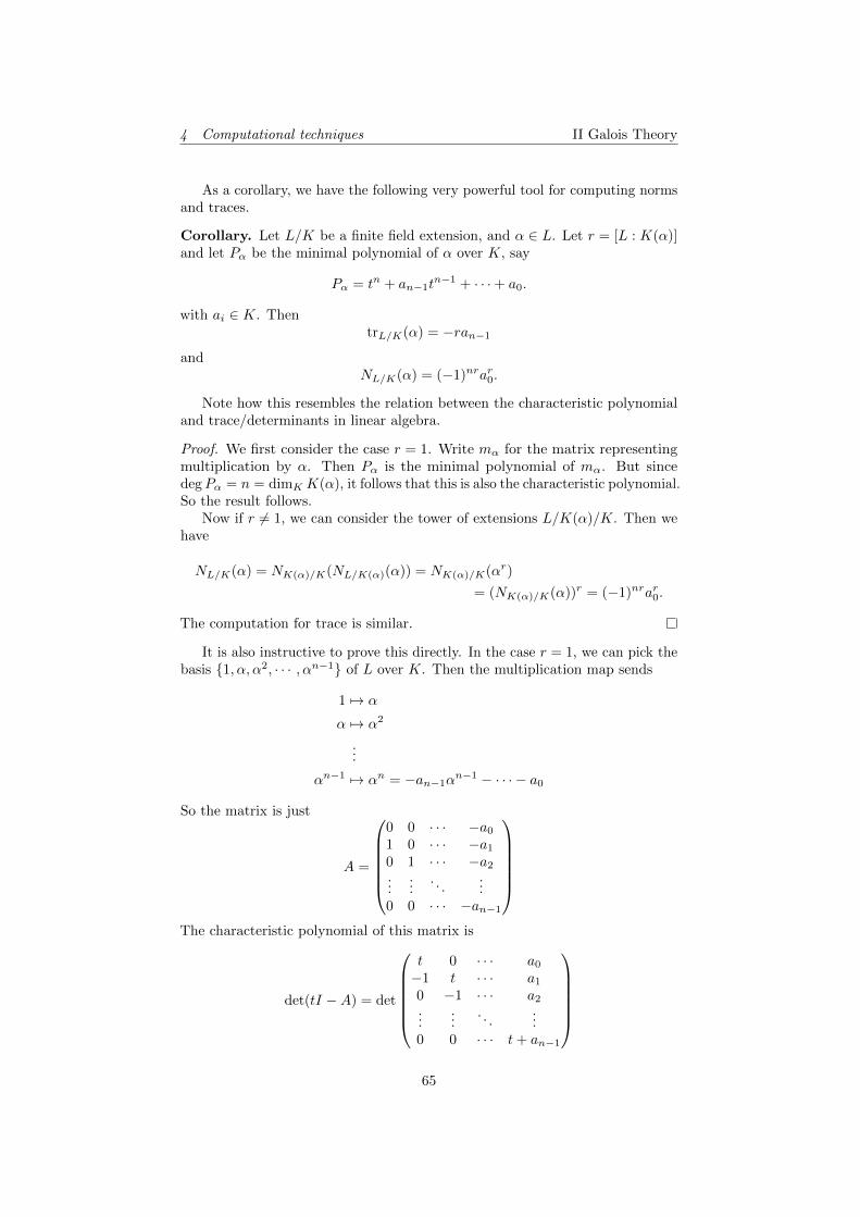
4 Computational techniques II Galois Theory
As a corollary, we have the following very powerful tool for computing normsand traces.
Corollary. Let L/K be a finite field extension, and α ∈ L. Let r = [L : K(α)]and let Pα be the minimal polynomial of α over K, say
Pα = tn + an−1tn−1 + · · ·+ a0.
with ai ∈ K. ThentrL/K(α) = −ran−1
andNL/K(α) = (−1)nrar0.
Note how this resembles the relation between the characteristic polynomialand trace/determinants in linear algebra.
Proof. We first consider the case r = 1. Write mα for the matrix representingmultiplication by α. Then Pα is the minimal polynomial of mα. But sincedegPα = n = dimK K(α), it follows that this is also the characteristic polynomial.So the result follows.
Now if r 6= 1, we can consider the tower of extensions L/K(α)/K. Then wehave
NL/K(α) = NK(α)/K(NL/K(α)(α)) = NK(α)/K(αr)
= (NK(α)/K(α))r = (−1)nrar0.
The computation for trace is similar.
It is also instructive to prove this directly. In the case r = 1, we can pick thebasis {1, α, α2, · · · , αn−1} of L over K. Then the multiplication map sends
1 7→ α
α 7→ α2
...
αn−1 7→ αn = −an−1αn−1 − · · · − a0
So the matrix is just
A =
0 0 · · · −a0
1 0 · · · −a1
0 1 · · · −a2
......
. . ....
0 0 · · · −an−1
The characteristic polynomial of this matrix is
det(tI −A) = det
t 0 · · · a0
−1 t · · · a1
0 −1 · · · a2
......
. . ....
0 0 · · · t+ an−1
65

4 Computational techniques II Galois Theory
By adding ti multiples of the ith row to the first row for each i, this gives
det(tI −A) = det
0 0 · · · Pα−1 t · · · a1
0 −1 · · · a2
......
. . ....
0 0 · · · t+ an−1
= Pα.
Then we notice that for r 6= 1, in an appropriate choice of basis, the matrixlooks like
C =
A 0 · · · 00 A · · · 0...
.... . .
...0 0 · · · A
.
Theorem. Let L/K be a finite but not separable extension. Then trL/K(α) = 0for all α ∈ L.
Proof. Pick β ∈ L such that Pβ , the minimal polynomial of β over K, is notseparable. Then by the previous characterization of separable polynomials, weknow p = charK > 0 with Pβ = q(tp) for some q ∈ K[t].
Now considerK ⊆ K(βp) ⊆ K(β) ⊆ L.
To show trL/K = 0, by the previous proposition, it suffices to show trK(β)/K(βp) =0.
Note that the minimal polynomial of βp over K is q because q(βp) = 0 and qis irreducible. Then [K(β) : K] = degPβ = pdeg q and deg[K(βp) : K] = deg q.So [K(β) : K(βp)] = p.
Now {1, β, β2, · · · , βp−1} is a basis of K(β) over K(βp). Let Rβi be theminimal polynomial of βi over K(βp). Then
Rβi =
{t− 1 i = 0
tp − βir i 6= 0,
We get the second case using the fact that p is a prime number, and henceK(βp)(βi) = K(β) if 1 ≤ i < p. So [K(βp)(βi) : K(βp)] = p and hence theminimal polynomial has degree p. Hence trK(β)/K(βp)(β
i) = 0 for all i.Thus, trK(β)/K(βp) = 0. Hence
trL/K = trK(βp)/K ◦ trK(β)/K(βp) ◦ trL/K(β) = 0.
Note that if L/K is a finite extension, and charK = 0, then
trL/K(1) = [L : K] 6= 0.
So trL/K 6= 0. It is in fact true that all separable extensions have trL/K 6= 0, notonly when the field has characteristic 0.
Example. We want to show 3√
3 6∈ Q( 3√
2). Suppose not. Then we haveL = Q( 3
√3) = Q( 3
√2), since both extensions of Q have degree 3. Then there
exists some a, b, c ∈ Q such that
3√
3 = a+ b3√
2 + c3√
22.
66

4 Computational techniques II Galois Theory
We now compute the traces over Q. The minimal polynomials over Q are
P 3√3 = t3 − 3, P 3√2 = t3 − 2, P 3√4 = t3 − 4.
So we have
trL/Q(3√
3) = a trL/Q(1) + b trL/Q(3√
2) + c trL/Q(3√
4).
Since the minimal polynomials above do not have coefficients in t2, the traces ofthe cube roots are zero. So we need a = 0. Then we are left with
3√
3 = b3√
2 + c3√
4.
We apply the same trick again. We multiply by 3√
2 to obtain
3√
6 = b3√
4 + 2c.
We note that the minimal polynomial of 3√
6 is t3 − 6. Taking the trace gives
trL/Q(3√
6) = b trL/Q(3√
4) + 6c.
Again, the traces are zero. So c = 0. So we have
3√
3 = b3√
2.
In other words,
b3 =3
2,
which is clearly nonsense. This is a contradiction. So 3√
3 6∈ Q( 3√
2).
We can obtain another formula for the trace and norm as follows:
Theorem. Let L/K be a finite separable extension. Pick a further extensionE/L such that E/K is normal and
|HomK(L,E)| = [L : K].
Write HomK(L,E) = {ϕ1, · · · , ϕn}. Then
trL/K(α) =
n∑i=1
ϕi(α), NL/K(α) =
n∏i=1
ϕi(α)
for all α ∈ L.
Proof. Let α ∈ L. Let Pα be the minimal polynomial of α over K. Then thereis a one-to-one correspondence between
HomK(K(α), E)←→ RootPα(E) = {α1, · · · , αd}.
wlog we let α = α1.Also, since
|HomK(L,E)| = [L : K],
we get|HomK(K(α), E)| = [K(α) : K] = degPα.
67

4 Computational techniques II Galois Theory
Moreover, the restriction map HomK(L,E) → HomK(K(α), E) (defined byϕ 7→ ϕ|K(α)) is surjective and sends exactly [K(α) : K] elements to any particularelement in HomK(K(α), E).
Therefore
∑ϕi(α) = [L : K(α)]
∑ψ∈HomK(K(α),E)
ψ(α) = [L : K(α)]
d∑i=1
αi.
Moreover, we can read the sum of roots of a polynomial is the (negative of the)coefficient of td−1, where
Pα = td + ad−1td−1 + · · ·+ a0.
So ∑ϕi(α) = [L : K(α)](−ad−1) = trL/K(α).
Similarly, we have
∏ϕi(α) =
∏ψ∈HomK(K(α),E)
ψ(α)
[L:K(α)]
=
(d∏i=1
αi
)[L:K(α)]
= ((−1)da0)[L:K(α)]
= NL/K(α).
Corollary. Let L/K be a finite separable extension. Then there is some α ∈ Lsuch that trL/K(α) 6= 0.
Proof. Using the notation of the previous theorem, we have
trL/K(α) =∑
ϕi(α).
Similar to a previous lemma, we can show that ϕ1, · · · , ϕn are “linearly indepen-dent” over E, and hence
∑ϕi cannot be identically zero. Hence there is some α
such thattrL/K(α) =
∑ϕi(α) 6= 0.
Example. Let K = Fq ⊆ L = Fqn , with q is a power of some prime number p.By a previous theorem on finite fields, we know L/K is Galois and
Gal(L/K) =ZnZ
and is generated by the Frobenius ϕ = Frq.To apply the theorem, we had to pick an E such that E/K is normal and
HomK(L,E) = [L : K]. However, since L/K is Galois, we can simply pickE = L.
68

4 Computational techniques II Galois Theory
Then we know
trL/K(α) =∑
ψ∈Gal(L/K)
ψ(α)
=
n−1∑i=0
ϕi(α)
= α+ αq + αq2
+ · · ·+ αqn−1
.
Similarly, the norm is
NL/K(α) =
n−1∏i=0
ϕi(α) = α · αq · · · · · αqn−1
.
Recall that when solving quadratic equations f = t2 + bt+ c, we defined thediscriminant as b2 − 4c. This discriminant then determined the types of roots off . In general, we can define the discriminant of a polynomial of any degree, in ascary way.
Definition (Discriminant). Let K be a field and f ∈ K[t], L the splitting fieldof f over K. So we have
f = a(t− α1) · · · (t− αn)
for some a, α1, · · · , αn ∈ L. We define
∆f =∏i<j
(αi − αj), Df = ∆2f = (−1)n(n−1)/2
∏i 6=j
(αi − αj).
We call Df the discriminant of f .
Clearly, Df 6= 0 if and only if f has no repeated roots.
Theorem. Let K be a field and f ∈ K[t], L is the splitting field of f over K.Suppose Df 6= 0 and charK 6= 2. Then
(i) Df ∈ K.
(ii) Let G = Gal(L/K), and θ : G → Sn be the embedding given by thepermutation of the roots. Then im θ ⊆ An if and only if ∆f ∈ K (if andonly if Df is a square in K).
Proof.
(i) It is clear that Df is fixed by Gal(L/K) since it only permutes the roots.
(ii) Consider a permutation σ ∈ Sn of the form σ = (` m), and let it act onthe roots. Then we claim that
σ(∆f ) = −∆f . (†)
So in general, odd elements in Sn negate ∆f while even elements fix it.Thus, ∆f ∈ K iff ∆f is fixed by Gal(L/K) iff every element of Gal(L/K)is even.
69

4 Computational techniques II Galois Theory
To prove (†), we have to painstakingly check all terms in the product. Wewlog ` < m. If k < `,m. Then this swaps (αk − α`) with αk − αm), whichhas no effect. The k > m case is similar. If ` < k < m, then this sends(α` − αk) 7→ (αm − αk) and (αk − αm) 7→ (α` − αm). This introduces twonegative signs, which has no net effect. Finally, this sends (αk − αm) toits negation, and so introduces a negative sign.
We will later use this result to compute certain Galois groups. Before that,we see how this discriminant is related to the norm.
Theorem. Let K be a field, and f ∈ K[t] be an n-degree monic irreduciblepolynomial with no repeated roots. Let L be the splitting field of f over K, andlet α ∈ RootF (L). Then
Df = (−1)n(n−1)/2NK(α)/K(f ′(α)).
Proof. Let HomK(K(α), L) = {ϕ1, · · · , ϕn}. Recall these are in one-to-onecorrespondence with Rootf (L) = {α1, · · · , αn}. Then we can compute∏
i6=j
(αi − αj) =∏i
∏j 6=i
(αi − αj).
Note that since f is just monic, we have
f = (t− α1) · · · (t− αn).
Computing the derivative directly, we find∏j 6=i
(αi − αj) = f ′(αi).
So we have ∏i6=j
(αi − αj) =∏i
f ′(αi).
Now since the ϕi just maps α to αi, we have∏i 6=j
(αi − αj) =∏i
ϕi(f′(α)) = NK(α)/K(f ′(α)).
Finally, multiplying the factor of (−1)n(n−1)/2 gives the desired result.
Example. Let K be a field with charK 6= 2, 3. Let f ∈ K[t] have degree 3, say
f = t3 + bt+ c
where we have gotten rid of the t2 term as in the first lecture. We further assumef is irreducible with no repeated roots, and let L be the splitting field of f .
We want to compute the discriminant of this polynomial. Let α ∈ Rootf (L).Then
β = f ′(α) = 3α2 + b.
Then we can see
β = −2b− 3c
α.
70

4 Computational techniques II Galois Theory
Alternatively, we have
α =−3c
β + 2b. (∗)
Putting (∗) into α3 + bα + c = 0, we find the minimal polynomial of β hasconstant term −4b3 − 27c2. This then gives us the norm, and we get
Df = −NK(α)/K(β) = −4b3 − 27c2.
This is the discriminant of a cubic.We can take a specific example, where
f = t3 − 31t+ 62.
Then f is irreducible over Q. We can compute Df , and find that it is a square.So the previous theorem says the image of the Galois group Gal(L/K) is asubgroup of A3. However, we also know Gal(L/K) has three elements sincedeg f = 3. So we know Gal(L/K) ∼= A3.
71