part I of a short course on The replica method and its ...

part I of a short course on

The replica method and its applications inbiomedical modelling and data analysis

ACC CoolenInstitute for Mathematical and Molecular Biomedicine, King’s College London

January 2014

ACC Coolen (IMMB@KCL) 1 / 67

replica methodA clever trick that enables the analytical calculation of averagesthat are normally impossible to do, except numerically.

is particularly useful forComplex heterogeneous systems composed of many interacting variables,and with many parameters on which we have only statistical information.(too large for numerical averages to be computationally feasible)

gives usAnalytical predictions for the behaviour of macroscopic quantitiesin typical realisations of the systems under study.

note on biomedical applicationsThe ‘large systems’ could describe actual biochemical processes(folding proteins, proteome, transcriptome, immune or neural networks, etc),or analysis algorithms running on large biomedical data sets


1 Mathematical preliminariesThe delta distributionGaussian integralsSteepest descent integration

2 The replica methodExponential families and generating functionsThe replica trickThe replica trick and algorithmsAlternative forms of the replica identity

3 Application: information storage in neural networksAttractor neural networksThe replica calculationReplica symmetryReplica symmetric solution

4 Application: overfitting transition in linear separatorsLinear separability of data – version spaceThe replica calculationGardner’s replica symmetric theoryOverfitting transition in Cox regression


The δ-distribution

intuitive definition of δ(x):

prob distribution for a ‘random’ variable xthat is always zero

〈f 〉 =

∫ ∞−∞

dx f (x)δ(x) = f (0) for any f

for instance

δ(x) = limσ→0

1σ√

2πe−x2/2σ2

0

1

2

3

-3 -2 -1 0 1 2 3

not a function: δ(x 6= 0) = 0, δ(0) =∞

status of δ(x):

δ(x) only has a meaning when appearing inside an integration,one takes the limit σ↓0 after performing the integration∫ ∞−∞

dx f (x)δ(x) = limσ↓0

∫ ∞−∞

dx f (x)e−x2/2σ2

σ√

2π= limσ↓0

∫ ∞−∞

dx f (xσ)e−x2/2

√2π

= f (0)


differentiation of δ(x):∫ ∞−∞

dx f (x)δ′(x) =

∫ ∞−∞

dx d

dx

(f (x)δ(x)

)− f ′(x)δ(x)

= lim

σ↓0

[f (x)

e−x2/2σ2

σ√

2π

]x=∞

x=−∞− f ′(0) = −f ′(0)

generalization:∫ ∞−∞

dx f (x)dn

dxn δ(x) = (−1)n limx→0

dn

dxn f (x) (n = 0, 1, 2, . . .)

integration of δ(x): δ(x) =d

dxθ(x)

θ(x<0) = 0θ(x>0) = 1

Proof: both sides have same effect in integrals∫dxδ(x)− d

dxθ(x)

f (x) = f (0)− lim

ε↓0

∫ ε

−εdx

ddx

(θ(x)f (x)

)− f ′(x)θ(x)

= f (0)− lim

ε↓0[f (ε)− 0] + lim

ε↓0

∫ ε

0dx f ′(x) = 0

generalizationto vector arguments: x ∈ IRN : δ(x) =

N∏i=1

δ(xi )


Integral representation of δ(x)

use defns of Fourier transforms and their inverse:

f (k) =∫∞−∞dx e−2πikx f (x)

f (x) =∫∞−∞dk e2πikx f (k)

⇒ f (x) =

∫ ∞−∞

dk e2πikx∫ ∞−∞

dy e−2πiky f (y)

apply to δ(x): δ(x) =

∫ ∞−∞

dk e2πikx =

∫ ∞−∞

dk2π

eikx

invertible functions of xas arguments: δ [g(x)− g(a)] =

δ(x − a)

|g′(a)|

Proof: both sides have same effect in integrals∫ ∞−∞

dx f (x)

δ [g(x)−g(a)]− δ(x−a)

|g′(a)|

=

∫ ∞−∞

dx g′(x)f (x)

g′(x)δ [g(x)−g(a)]− f (a)

|g′(a)|

=

∫ g(∞)

g(−∞)

dkf (ginv(k))

g′(ginv(k))δ [k−g(a)]− f (a)

|g′(a)|

= sgn[g′(a)]

∫ ∞−∞

dkf (ginv(k))

g′(ginv(k))δ [k−g(a)]− f (a)

|g′(a)|

= sgn[g′(a)]f (a)

g′(a)− f (a)

|g′(a)| = 0


Gaussian integrals

one-dimensional:∫dx

σ√

2πe−

12 x2/σ2

= 1,∫

dxσ√

2πx e−

12 x2/σ2

= 0,∫

dxσ√

2πx2e−

12 x2/σ2

= σ2

∫dx√2π

ekx− 12 x2

= e12 k2

(k ∈ |C)

N-dimensional:∫dx√

(2π)NdetCe−

12 x·C−1x = 1,

∫dx√

(2π)NdetCxie−

12 x·C−1x = 0,

∫dx√

(2π)NdetCxixje−

12 x·C−1x = Cij

multivariateGaussiandistribution:

p(x) =1√

(2π)NdetCe−

12 x·C−1x

∫dx p(x)xixj = Cij ,

∫dx p(x)eik·x = e−

12 k·Ck


Steepest descent integration

Objective of steepest descent(or ‘saddle-point’) integration:large N behavior of integrals of the type IN =

∫IRp

dx g(x) e−Nf (x)

f (x) real-valued, smooth, bounded from below,and with unique minimum at x?

expand f around minimum:

f (x) = f (x?) +12

p∑ij=1

Aij (xi−x?i )(xj−x?j ) +O(|x−x?|3) Aij =∂2f∂xi∂xj

∣∣∣∣x?

Insert into integral,transform x = x?+y/

√N:

IN = e−Nf (x?)

∫IRp

dx g(x)e−12 N

∑ij (xi−x?i )Aij (xj−x?j )+O(N|x−x?|3)

= N−p2 e−Nf (x?)

∫IRp

dy g(

x?+y√N

)e−

12∑

ij yi Aij yj +O(|y|3/√

N)


∫IRp

dx g(x) e−Nf (x) = N−p2 e−Nf (x?)

∫IRp

dy g(

x?+y√N

)e−

12∑


N)

first result, for p N/ log N:

− limN→∞

1N

log∫

IRpdx e−Nf (x)

= f (x?) + limN→∞

[p log N

2N− 1

Nlog∫

IRpdy e−

12∑


N)

]= f (x?) + lim

N→∞

[p log N

2N− 1

2Nlog( (2π)p

det A

)− 1

Nlog(

1+O(p3/2

√N

))]

= f (x?) + limN→∞

[p log N

2N+O(

pN

) +O(p3/2

N3/2 )

]= f (x?)

second result, for p √

N:

limN→∞

∫dx g(x)e−Nf (x)∫

dx e−Nf (x)= lim

N→∞

[∫IRp dy g(x?+y/

√N) e−

12∑


N)∫IRp dy e−

12∑


N)

]

=g(x?)

(1 +O( p√

N))√

(2π)p

det A

(1+O( p3/2

√N

))

√(2π)p

det A

(1+O( p3/2

√N

)) = g(x?)


f (x) complex-valued:

– deform integration path in complex plane, using Cauchy’s theorem, such thatalong deformed path the imaginary part of f (x) is constant, and preferably zero

– proceed using Laplace’s argument, and find the leading order in N byextremization of the real part of f (x)

similar fomulae,but with (possibly complex) extremathat need no longer be maxima:

− limN→∞

1N

log∫

IRpdx e−Nf (x) = extrx∈IRp f (x)

limN→∞

∫IRp dx g(x)e−Nf (x)∫

IRp dx e−Nf (x)= g

(arg extrx∈IRp f (x)

)


Exponential distributionsOften we study stochastic processes for x ∈ X ⊆ IRN ,that evolve to a stationary state, with prob distribution p(x)many are of the following form:

stationary state is minimally informative,subject to a number of constraints∑

x∈X

p(x)ω1(x) = Ω1 . . . . . .∑x∈X

p(x)ωL(x) = ΩL

This is enough to calculate p(x):

information content of x: Shannon entropyhence

maximize S = −∑x∈X

p(x) log p(x)

subject to :

p(x) ≥ 0 ∀x,

∑x∈X p(x) = 1∑

x∈X p(x)ω`(x) = Ω` for all ` = 1 . . . L


solution using Lagrange’s method:

∂

∂p(x)

λ0

∑x′∈X

p(x′) +L∑`=1

λ`∑x′∈X

p(x′)ω`(x′)−∑x′∈X

p(x′) log p(x′)

= 0

λ0 +L∑`=1

λ`ω`(x)− 1− log p(x) = 0 ⇒ p(x) = eλ0−1+∑L`=1 λ`ω`(x)

(p(x) ≥ 0 automatically satisfied)

‘exponential distribution’:

p(x) =e∑L`=1 λ`ω`(x)

Z (λ), Z (λ) =

∑x∈X

e∑L`=1 λ`ω`(x)

λ = (λ1, . . . , λL) : solved from∑x∈X

p(x)ω`(x) = Ω` (` = 1 . . . L)

example:physical systems in thermal equilibriumL = 1, ω(x) = E(x) (energy), λ = −1/kBT

p(x) =e−E(x)/kBT

Z (T ), Z (T ) =

∑x∈X

e−E(x)/kBT


Generating functions

p(x) =e∑L`=1 λ`ω`(x)

Z (λ), Z (λ) =

∑x∈X

e∑L`=1 λ`ω`(x), 〈f 〉 =

∑x∈X

p(x)f (x)

Idea behind generating functions:reduce nr of state averages to be calculated ...

defineF (λ) = log Z (λ) ∂F (λ)

∂λk=

∑x∈X ωk (x)e

∑L`=1 λ`ω`(x)∑

x∈X e∑L`=1 λ`ω`(x)

= 〈ωk (x)〉

how to calculatearbitrary state average 〈ψ〉?

F (λ, µ) = log[∑

x∈X

eµψ(x)+∑` λ`ω`(x)

]〈ψ〉 = lim

µ→0

∂F (λ, µ)

∂µ, 〈ω`〉 = lim

µ→0

∂F (λ, µ)

∂λ`


The replica trick

first appearance: Marc Kac 1968first application in physics: Sherrington & Kirkpatrick 1975first application in biology: Amit, Gutfreund & Sompolinksy 1985

Consider processes with manyfixed (pseudo-)random parameters ξ,distributed according to P(ξ)

p(x|ξ) =e∑L`=1 λ`ω`(x,ξ)

Z (λ, ξ), Z (λ, ξ) =

∑x∈X

e∑L`=1 λ`ω`(x,ξ)

– calculating state averages 〈f 〉ξ for each realisation of ξ is usually impossible

– we are mostly interested in typical values of state averages– for N→∞ macroscopic averages will not depend on ξ, only on P(ξ),

‘self-averaging’: limN→∞〈f 〉ξ indep of ξ

so focus on

〈f 〉ξ =∑ξ

P(ξ)〈f 〉ξ =∑ξ

P(ξ)∑

x∈X

p(x|ξ)f (x, ξ)


new generating function:

F (λ, µ) =∑ξ

P(ξ) log Z (λ, µ, ξ), Z (λ, µ, ξ) =∑x∈X

eµψ(x,ξ)+∑` λ`ω`(x,ξ)

limµ→0

∂

∂µF (λ, µ) = lim

µ→0

∑ξ

P(ξ)

∑x∈X ψ(x, ξ)eµψ(x,ξ)+

∑` λ`ω`(x,ξ)∑

x∈X eµψ(x,ξ)+∑` λ`ω`(x,ξ)

=∑ξ

P(ξ)

∑x∈X ψ(x, ξ)e

∑` λ`ω`(x,ξ)∑

x∈X e∑` λ`ω`(x,ξ)

= 〈ψ〉ξ

main obstacle in calculating F :the logarithm ...

replica identity : log Z = limn→0

1n

log Z n

proof:

limn→0

1n

log Z n = limn→0

1n

log [en log Z ] = limn→0

1n

log [1 + n log Z +O(n2)]

= limn→0

1n

log[1 + nlog Z +O(n2)] = log Z


apply log Z = limn→01n log Z n

(simplest case L = 1)

F (λ) =∑ξ

P(ξ) log[∑

x∈X

eλω(x,ξ)]

= limn→0

1n

log∑ξ

P(ξ)[∑

x∈X

eλω(x,ξ)]n

= limn→0

1n

log∑ξ

P(ξ)[ ∑

x1∈X

. . .∑xn∈X

eλ∑nα=1 ω(xα,ξ)

]= lim

n→0

1n

log[ ∑

x1∈X

. . .∑xn∈X

∑ξ

P(ξ)eλ∑nα=1 ω(xα,ξ)

]

notes:

– impossible ξ-average converted into simpler one ...– calculation involves n ‘replicas’ xα of original system– but n→ 0 at the end ... ?– penultimate step true only for integer n,

so limit requires analytical continuation ...

since then: alternative (more tedious) routes,these confirmed correctness of the replica method!


The replica trick and algorithms

Suppose we have data D, with prob distr P(D)and an algorithm which minimises an error function E(D,θ)(maximum likelihood, Cox & Bayesian regression, SVM, perceptron, ...)

algorithm outcome:

θ?(D) = arg minθE(D,θ), Emin(D) = minθE(D,θ)

typical performance:

θ? =∑

D

P(D)θ?(D) = θ?(D) Emin =∑

D

P(D)Emin(D) = Emin(D)

steepest descent identity & replica trick:

Emin(D) = minθE(D,θ) = − limβ→∞

1β

log∫

dθ e−βE(D,θ)

Emin = Emin(D) = − limβ→∞

1β

log∫

dθ e−βE(D,θ)

= − limβ→∞

limn→0

1βn

log[ ∫

dθ e−βE(D,θ)]n

= − limβ→∞

limn→0

1βn

log∫

dθ1. . .θn e−β∑nα=1 E(D,θα)


Alternative forms of the replica identity

suppose we need averages, but fora p(x|ξ) that is not of an exponential form?

or we need to average quantities that wedon’t want in the exponent of Z (λξ)?

p(x|ξ) =W (x, ξ)∑

x′∈X W (x′, ξ), 〈f 〉ξ =

∑x∈X

p(x|ξ)f (x, ξ)

main obstacle here:the fraction ...

〈f 〉ξ =[∑

x∈X W (x, ξ)f (x, ξ)∑x∈X W (x, ξ)

]=[∑

x∈X

W (x, ξ)f (x, ξ)][∑

x∈X

W (x, ξ)]−1

= limn→0

[∑x∈X

W (x, ξ)f (x, ξ)][∑

x∈X

W (x, ξ)]n−1

= limn→0

∑x1∈X

. . .∑xn∈X

f (x1, ξ)W (x1, ξ) . . .W (xn, ξ)

(again: used integer n, but n→ 0 ...)ACC Coolen (IMMB@KCL) 25 / 67

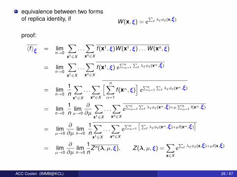
equivalence between two formsof replica identity, if W (x, ξ) = e

∑` λ`φ`(x,ξ)

proof:

〈f 〉ξ = limn→0

∑x1∈X

. . .∑xn∈X

f (x1, ξ)W (x1, ξ) . . .W (xn, ξ)

= limn→0

∑x1∈X

. . .∑xn∈X

f (x1, ξ) e∑nα=1

∑` λ`φ`(xα,ξ)

= limn→0

1n

∑x1∈X

. . .∑xn∈X

[ n∑α=1

f (xα, ξ)]

e∑nα=1

∑` λ`φ`(xα,ξ)

= limn→0

1n

limµ→0

∂

∂µ

∑x1∈X

. . .∑xn∈X

e∑nα=1

∑` λ`φ`(xα,ξ)+µ

∑nα=1 f (xα,ξ)

= limµ→0

∂

∂µlimn→0

1n

∑x1∈X

. . .∑xn∈X

e∑nα=1

[∑` λ`φ`(xα,ξ)+µf (xα,ξ)

]= lim

µ→0

∂

∂µlimn→0

1n

Z n(λ, µ, ξ), Z (λ, µ, ξ) =∑x∈X

e∑` λ`φ`(x,ξ)+µf (x,ξ)


Attractor neural networks

N∼1012−14 brain cells (neurons),each connected with ∼103−5 others

neurons

two states:σi = 1 (i fires electric pulses)σi = −1 (i is at rest)

dynamics of firing states

σi (t +1) = sgn[ activation signal︷︸︸︷

N∑j=1

Jijσj (t) +

threshold, noise︷︸︸︷θi + zi (t)

]θi ∈ IR: firing threshold of neuron i non-local ‘distributed’ storage ofJij ∈ IR: synaptic connection j → i ‘program’ and ‘data’

learning = adaptation of Jij , θi


attractor neural networksmodels for associative memory in the brain

the neural coderepresent ‘patterns’ asmicro-states ξ = (ξ1, . . . , ξN) : σi =−1, • : σi =1

e.g. N =400,10 patterns:

information storagemodify synapses Jij such that ξ isstable state (attractor) of the neuronal dynamics

information recallinitial state σ(t =0):evolution to nearest attractor

if σ(0) close (i.e. similar) to ξ:σ(t =∞) = ξ


learning rule: recipe for storing patterns via modification of JijHebb (1949): ∆Jij ∝ ξiξj

choose Jij =J0ξiξj , θi =0,update randomly drawn i at each step:

σi (t +1) = sgn[ N∑

j=1

Jijσj (t) + zi (t)]

= sgn[J0ξi

( pattern overlap︷︸︸︷N∑

j=1

ξjσj (t))

+ zi (t)]

= ξi sgn[J0

N∑j=1

ξjσj (t) + ξizi (t)]

M(t) =∑N

j=1 ξjσj (t) sufficiently large: σi (t +1) = ξi

now M(t +1) ≥ M(t) ...will continue until σ = ξ

proper analysis:

noise: P(z) = β2 [1−tanh2(βz)],

symmetric synapses: Jij = Jji , Jii = 0sequential updates of σi

p(σ) =e−βH(σ)

Z (β), H(σ) = −1

2

∑i 6=j

σiJijσj −∑

i

θiσi


a more realistic model,solvable via the replica method

storage of a pattern ξ = (ξ1, . . . , ξN) ∈ −1, 1N

on background of zero-average Gaussian synapses

Jij =J0

Nξiξj +

J√N

zij , z ij = 0, zij2 = 1, J, J0 ≥ 0, θi = 0

to be averaged over: background synapses zijpattern overlap: m(σ) = 1

N

∑k σkξk

H(σ) = −12

∑i 6=j

σiσj

J0

Nξiξj +

J√N

zij

= − J0

2N

∑ij

σiσjξiξj +J0

2N

∑i

1− J2√

N

∑i 6=j

σiσjzij

= −12

NJ0m2(σ) +12

J0 −J√N

∑i<j

σiσjzij

generating function

F = log Z (β) = limn→0

1n

log Z n(β) = limn→0

1n

log[ ∑σ1...σn

e−β∑nα=1 H(σα)

]ACC Coolen (IMMB@KCL) 31 / 67

The replica calculation

short-hands: m(σ) = 1N

∑i ξiσi , Dz = (2π)−1/2e−z2/2dz

Gaussian integral:∫

Dz exz = e12 x2

average over random synapses

Z n(β) =∑

σ1...σn

e−β∑nα=1 H(σα)

=∑

σ1...σn

e−β∑nα=1

[12 J0− 1

2 NJ0m2(σα)− J√N

∑i<j σ

αi σ

αj zij

]

= e−12 nβJ0

∑σ1...σn

e12 NβJ0

∑nα=1m2(σα)e

βJ√N

∑nα=1

∑i<j σ

αi σ

αj zij

= e−12 nβJ0

∑σ1...σn

e12 NβJ0

∑nα=1m2(σα)

∏i<j

∫Dz e

βJ√N

∑nα=1σ

αi σ

αj z

= e−12 nβJ0

∑σ1...σn

e12 NβJ0

∑nα=1m2(σα)

∏i<j

eβ2J2

2N

[∑nα=1σ

αi σ

αj

]2

= e−12 nβJ0

∑σ1...σn

eN[

12βJ0

∑nα=1m2(σα)+ 1

2 (βJ)2 ∑nα,γ=1

(N−2 ∑

i<j σαi σ

αj σ

γi σ

γj

)]ACC Coolen (IMMB@KCL) 33 / 67

complete square in sums over neurons∑i<j

σαi σαj σ

γi σ

γj =

12

∑i 6=j

σαi σαj σ

γi σ

γj =

12

∑ij

σαi σαj σ

γi σ

γj −

12

∑i

1

=12

(∑i

σαi σγi

)2− 1

2N

hence

Z n(β) = e−12 nβJ0

∑σ1...σn

eN[

12βJ0

∑nα=1m2(σα)+ 1

4 (βJ)2 ∑nα,γ=1

((1N

∑i σαi σ

γi

)2− 1

N

)]= e−

12 nβJ0− 1

4 n(βJ)2 ∑σ1...σn

eN[

12βJ0

∑nα=1m2(σα)+ 1

4 (βJ)2 ∑nα,γ=1

(1N

∑i σαi σ

γi

)2]

insert:

1 =n∏α=1

∫dmα δ

(mα−

1N

∑i

ξiσαi

), 1 =

n∏α,γ=1

∫dqαγ δ

(qαγ−

1N

∑i

σαi σγi

)m∈ IRn, q∈ IRn2

:

Z n(β) = e−12 nβJ0− 1

4 n(βJ)2∫

dmdq eN[

12βJ0

∑nα=1m2

α+ 14 (βJ)2 ∑n

α,γ=1 q2αγ

]×

∑σ1...σn

[ n∏α=1

δ(

mα−1N

∑i

ξiσαi

)][ n∏α,γ=1

δ(

qαγ−1N

∑i

σαi σγi

)]ACC Coolen (IMMB@KCL) 34 / 67

remember: δ(x) = (2π)−1 ∫ dx eixx

the sum over neuron state variables∑σ1...σn

[ n∏α=1

δ(

mα−1N

∑i

ξiσαi

)][ n∏α,γ=1

δ(

qαγ−1N

∑i

σαi σγi

)]=

∑σ1...σn

∫dmdq

(2π)n2+nei

∑nα=1 mα

[mα− 1

N∑

i ξiσαi

]+i

∑nα,γ=1 qαγ

[qαγ− 1

N∑

i σαi σ

γi

]

=

∫dmdq

(2π)n(n+1)ei

∑α mαmα+i

∑αγ qαγqαγ

∑σ1...σn

N∏i=1

e−iN

[∑α mαξiσ

αi +

∑αγ qαγσαi σ

γi

]=

∫dmdq

(2π)n(n+1)ei

∑α mαmα+i

∑αγ qαγqαγ

∏i

∑σ1...σn

e−iN

[∑α mαξiσα+

∑αγ qαγσασγ

]

transform: m→ Nm, q→ Nq, σα → ξiσα:∑σ1...σn

[. . .][. . .]

=

∫dmdq

(2π/N)n(n+1)eiN[

m·m+Tr(qq)][ ∑

σ∈−1,1n

e−im·σ−iσ·qσ]N

=

∫dmdq

(2π/N)n(n+1)eiNm·m+iNTr(qq)+N log

∑σ exp(−im·σ−iσ·qσ)


combine everything ...

Z n(β) = e−12 nβJ0− 1

4 n(βJ)2−n(n+1) log(2π/N)

∫dmdqdmdq eNΨ(m,q,m,q)

Ψ(. . .) =12βJ0m2 +

14

(βJ)2Tr(q2) + im ·m + iTr(qq) + log∑σ

e−im·σ−iσ·qσ

Hence

F = limn→0

1n

log Z n(β)

= −12βJ0 −

14

(βJ)2 − log(2πN

) + limn→0

1n

log∫

dmdqdmdq eNΨ(m,q,m,q)

Since F = O(N),large N behaviour follows from

f = limN→∞

F/N = limN→∞

limn→0

1nN

log∫

dmdqdmdq eNΨ(m,q,m,q)

assume limits commute,steepest descent integration: f = lim

n→0

1n

extrm,q,m,qΨ(m,q, m, q)


Ψ(. . .) =12βJ0

∑α

m2α +

14

(βJ)2∑αγ

q2αγ + i

∑α

mαmα + i∑αγ

qαγqαγ

+ log∑σ

e−i∑λ mλσλ−i

∑λζ σλqλζσζ

saddle-point eqns

∂Ψ

∂mα= 0,

∂Ψ

∂qαγ= 0 : βJ0mα + imα = 0,

12

(βJ)2qαγ + iqαγ = 0

∂Ψ

∂mα= 0 : imα − i

∑σ σαe−i

∑λ mλσλ−i

∑λζ σλqλζσζ∑

σ e−i∑λ mλσλ−i


= 0

∂Ψ

∂qαγ= 0 : iqαγ − i

∑σ σασγe−i

∑λ mλσλ−i

∑λζ σλqλζσζ∑

σ e−i∑λ mλσλ−i


= 0

eliminate (m, q)

mα =

∑σ σαeβJ0

∑λ mλσλ+ 1

2 (βJ)2 ∑λ 6=ζ σλqλζσζ∑

σ eβJ0∑λ mλσλ+ 1

2 (βJ)2 ∑λ 6=ζ σλqλζσζ

qαγ =

∑σ σασγeβJ0

∑λ mλσλ+ 1

2 (βJ)2 ∑λ6=ζ σλqλζσζ∑

σ eβJ0∑λ mλσλ+ 1

2 (βJ)2 ∑λ 6=ζ σλqλζσζtrivial soln: m=q=0,

any others?ACC Coolen (IMMB@KCL) 37 / 67

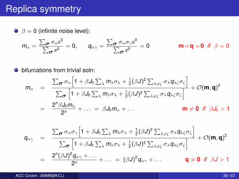
Replica symmetry

β = 0 (infinite noise level):

mα =

∑σ σαe0∑σ e0 = 0, qαγ =

∑σ σασγe0∑

σ e0 = 0 m=q =0 if β = 0

bifurcations from trivial soln:

mα =

∑σ σα

[1 + βJ0

∑λ mλσλ + 1

2 (βJ)2∑λ 6=ζ σλqλζσζ

]∑

σ

[1 + βJ0

∑λ mλσλ + 1

2 (βJ)2∑λ6=ζ σλqλζσζ

] +O(m,q)2

=2nβJ0mα

2n + . . . = βJ0mα + . . . m 6= 0 if βJ0 > 1

qαγ =

∑σ σασγ

[1 + βJ0

∑λ mλσλ + 1


]∑

σ

[1 + βJ0

∑λ mλσλ + 1


] +O(m,q)2

=2n(βJ)2qαγ + . . .

2n + . . . = (βJ)2qαγ + . . . q 6= 0 if βJ > 1


how to find form of nontrivial solns mα, qαγ?need their physical interpretation!use alternative form(s) of replica identity:

〈f (σ)〉 = limn→0

1n

n∑γ=1

∑σ1

. . .∑σn

f (σγ)e−β∑nα=1 H(σα)

〈〈f (σ,σ′)〉〉 = limn→0

1n(n−1)

n∑α 6=γ=1

∑σ1

. . .∑σn

f (σα,σγ)e−β∑nα=1 H(σα)

apply toP(m|σ) = δ

[m − 1

N

N∑i=1

ξiσi

], P(q|σ,σ′) = δ

[q − 1

N

N∑i=1

σiσ′i

]repeat steps of previous calculation,gives expressions in terms ofsaddle-point soln mα, qαγ:

limN→∞

〈P(m|σ)〉 = limn→0

1n

n∑α=1

δ[m−mα]

limN→∞

〈〈P(q|σ,σ′)〉〉 = limn→0

1n(n−1)

n∑α 6=γ=1

δ[q−qαγ ]


ergodic mean-field systems

fluctuations in quantities like 1N

∑Ni=1 ξiσi

or 1N

∑Ni=1 σiσ

′i scale as O(N−1/2)

hence

limN→∞

〈P(m|σ)〉 = limN→∞

⟨δ[m − 1

N

N∑i=1

ξiσi

]⟩= δ[m − 1

N

N∑i=1

ξi〈σi〉]

limN→∞

〈〈P(q|σ,σ′)〉〉 = limN→∞

⟨⟨δ[q − 1

N

N∑i=1

σiσ′i

]⟩⟩= δ[q − 1

N

N∑i=1

〈σi〉2]

hence

∀α : mα = m = limN→∞

1N

N∑i=1

ξi〈σi〉

∀α 6= γ : qαγ = q = limN→∞

1N

N∑i=1

〈σi〉2

replica-symmetric solution


Replica symmetric solution

mα = m, qα 6=β = q, now find m and q ...

RS saddle-point eqnsinsert RS form and use exp( 1

2 x2) =∫

Dz exz

m =

∑σ σαeβJ0m

∑λ σλ+ 1

2 (βJ)2q∑λ 6=ζ σλσζ∑

σ eβJ0m∑λ σλ+ 1

2 (βJ)2q∑λ6=ζ σλσζ

=

∑σ σαeβJ0m

∑λσλ+ 1

2 (βJ)2q[∑λσλ]2∑

σ eβJ0m∑λσλ+ 1

2 (βJ)2q[∑λσλ]2

=

∫Dz∑

σ σα∏nλ=1 eβ(J0m+Jz

√q)σλ∫

Dz∑

σ∏nλ=1 eβ(J0m+Jz

√q)σλ

=

∫Dz sinh[β(J0m+Jz

√q)] coshn−1[β(J0m+Jz

√q)]∫

Dz coshn[β(J0m+Jz√

q)]

similarlyq =

∫Dz sinh2[β(J0m+Jz

√q)] coshn−2[β(J0m+Jz

√q)]∫

Dz coshn[β(J0m+Jz√

q)]

the limit n→ 0

m =

∫Dz tanh[β(J0m+Jz

√q)], q =

∫Dz tanh2[β(J0m+Jz

√q)]


RS equations for m = limN→∞1N

∑Ni=1 ξi〈σi〉

and q = limN→∞1N

∑Ni=1 〈σi〉2

m =


√q)], q =


√q)]

bifurcations away from (m, q) = (0, 0):

m =

∫Dz[βJ0m+βJz

√q+O(m,

√q)3] = βJ0m + . . .

q =

∫Dz[βJ0m+βJz

√q+O(m,

√q)3]2 =

∫Dz (βJ)2z2q + . . .

= (βJ)2q + . . .

hence:first continuous bifurcations away from q=m=0,as identified earlier, are the RS solutions


m = limN→∞

1N

N∑i=1

ξi〈σi〉, q = limN→∞

1N

N∑i=1

〈σi〉2

m =


√q)], q =


√q)]

phase diagram

P: m = q = 0random neuronal firing

SG: m = 0, q > 0stable firing patterns, butnot related to stored pattern

F: m, q > 0recall of stored information

T = 1/β (noise strength)

βJ = 1

βJ0 = 1


Linear separability of data and version space

Dimension mismatch and overfitting

two clinical outcomes (A,B),4 patients, 60 expression levels ...

A : (100101001010010101010010001010111001001001001001001000011111)A : (010001000010101001010101010010101000111100101001001010101000)B : (001010001110101101100100100111001110010100101010101000101010)B : (101011001010110010100100111100100101100111010111010001010010)

prognostic signature!A : (100101001010010101010010001010111001001001001001001000011111)A : (010001000010101001010101010010101000111100101001001010101000)B : (001010001110101101100100100111001110010100101010101000101010)B : (101011001010110010100100111100100101100111010111010001010010)

shuffle outcome labels ...A : (100101001010010101010010001010111001001001001001001000011111)B : (010001000010101001010101010010101000111100101001001010101000)A : (001010001110101101100100100111001110010100101010101000101010)B : (101011001010110010100100111100100101100111010111010001010010)

overfitting, no reproducibility ...how about overfitting in regression?


Suppose we have data D on N patients,pairs of covariate vectors + clinical outcome labels

D = (x1, t1), . . . , (xN , tN), xi ∈ −1, 1p, t i ∈ −1, 1, p,N 1

e.g. xi= gene expressions of i (on/off)t i= treatment response of i (yes/no)

assumed model:

t(x) =

1 if

∑pµ=1 θµxµ > 0

−1 if∑pµ=1 θµxµ < 0

= sgn[ p∑µ=1

θµxµ]

+ : t i = 1o : t i =−1

regression/classification task:find parameters θ = (θ1 . . . , θp)such that for all i = 1 . . .N : t i = sgn

[ p∑µ=1

θµx iµ

]


data D explained perfectly by θ if

for all i = 1 . . .N : t i = sgn[θ · xi], i .e. t i (θ · xi ) > 0

separating plane in input space : θ · x = 0

distance ∆i between xi and separating plane : di = t i (θ · xi )/|θ||θ| irrelevant , so choose |θ|2 = p

version space

all θ that solve above eqnswith distances κ or larger

volume of version space:V (κ) =

∫dθ δ(θ2−p)

N∏i=1

θ[ t i (θ · xi )√

p> κ

]

high dimensional data: p large, α = N/pV (κ) scales exponentially with p, so

F =1p

log V (κ) =1p

log∫

dθ δ(θ2−p)N∏

i=1

θ[ t i (θ · xi )√

p> κ

]F = −∞: no solutions θ exist, data D not linearly separableF = finite: solutions θ exist, data D linearly separable


overfitting: find parameters θ that ‘explain’ random patternswhat if we choose random data D?

D = (x1, t1), . . . , (xN , tN), xi ∈ −1, 1p, t i ∈ −1, 1, fully random

typical classificationperformance:

F =1p

log∫

dθ δ(p−θ2)N∏

i=1

θ[ t i (θ · xi )√

p> κ

]

=1p

log∫

dz2π

eizp

∫dθ e−izθ2

N∏i=1

θ[ t i (θ · xi )√

p> κ

]

transport data vars to harmless place,using δ-functions, by inserting

1 =

∫dyi δ

[yi −

t i (θ · xi )√p

]=

∫dyi dyi

2πeiyi yi−iyi t

i (θ·xi )/√

p

gives

F =1p

log∫

dzdydydθ(2π)N+1 eizp+iy·y−izθ2

( N∏i=1

θ(yi−κ)e−iyi t i (θ·xi )/√

p)


The replica calculation

large p, large N,N = αp:

F = limp→∞

1p

log∫

dzdydydθ(2π)N+1 eizp+iy·y−izθ2

( N∏i=1


p)

replica identity

log Z = limn→0 n−1 log Z n

F = limp→∞

limn→0

1pn

log[ ∫ dzdydydθ

(2π)N+1 eizp+iy·y−izθ2( N∏

i=1


p)]n

= limp→∞

limn→0

1pn

log∫ n∏α=1

[dzαdyαdyαdθα

(2π)N+1 eipzα+iyα·yα−izα(θα)2N∏

i=1

θ[yαi −κ]]

×e−i∑N

i=1∑nα=1 yαi t i (θα·xi )/

√p


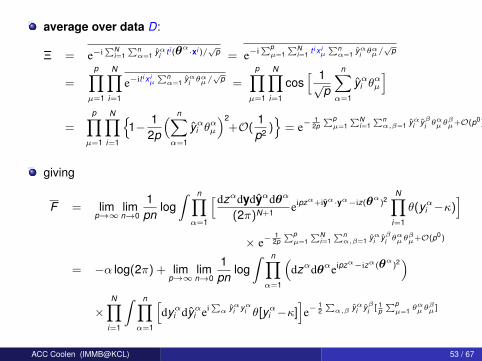
average over data D:

Ξ = e−i∑N

i=1∑nα=1 yαi t i (θα·xi )/

√p = e−i

∑pµ=1

∑Ni=1 t i x i

µ

∑nα=1 yαi θ

αµ/√

p

=

p∏µ=1

N∏i=1

e−it i x iµ

∑nα=1 yαi θ

αµ/√

p =

p∏µ=1

N∏i=1

cos[ 1√

p

n∑α=1

yαi θαµ

]

=

p∏µ=1

N∏i=1

1− 1

2p

( n∑α=1

yαi θαµ

)2+O(

1p2 )

= e−1

2p∑pµ=1

∑Ni=1

∑nα,β=1 yαi yβi θ

αµθβµ+O(p0)

giving

F = limp→∞

limn→0

1pn

log∫ n∏α=1

[dzαdydyαdθα

(2π)N+1 eipzα+iyα·yα−iz(θα)2N∏

i=1

θ(yαi −κ)]

× e−1

2p∑pµ=1

∑Ni=1

∑nα,β=1 yαi yβi θ

αµθβµ+O(p0)

= −α log(2π) + limp→∞

limn→0

1pn

log∫ n∏α=1

(dzαdθαeipzα−izα(θα)2

)

×N∏

i=1

∫ n∏α=1

[dyαi dyαi ei

∑α yαi yαi θ[yαi −κ]

]e−

12∑α,β yαi yβi [ 1

p∑pµ=1 θ

αµθβµ ]


so, with y = (y1, . . . , yn), y = (y1, . . . , yn),z = (z1, . . . , zn):

F = −α log(2π) + limp→∞

limn→0

1pn

log∫

dz( n∏α=1

dθαeipzα−izα(θα)2)

×∫

dydy eiy·yn∏α=1

θ[yα−κ] e−12∑α,β yα yβ [ 1

p∑pµ=1 θ

αµθβµ ]N

insert

1 =

∫dqαβ δ

[qαβ −

1p

p∑µ=1

θαµθβµ

]=

∫dqαβdqαβ

2π/pe

ipqαβ

[qαβ− 1

p∑pµ=1 θ

αµθβµ

]

to get


limn→0

1pn

log∫

dzdqdq eip∑nαβ=1 qαβqαβ+ip

∑nα=1 zα

×∫

dydy eiy·yn∏α=1

θ[yα−κ] e−12 y·qy

N∫ n∏α=1

(dθαe−izα(θα)2

)e−i

∑pµ=1

∑αβ qαβθ

αµθβµ


so, with θ = (θ1, . . . , θn):(remember: N = αp)


limn→0

1pn

log∫

dzdqdq eip∑nαβ=1 qαβqαβ+ip

∑nα=1 zα

×∫

dydy eiy·yn∏α=1

θ[yα−κ] e−12 y·qy

αp∫dθ e−i

∑nα=1 zαθ2

α−iθ·qθp

= limp→∞

limn→0

1pn

log∫

dzdqdq epΨ(z,q,q)

Ψ(. . .) = in∑

αβ=1

qαβqαβ + in∑α=1

zα + log∫

dθ e−i∑nα=1 zαθ2

α−iθ·qθ

+α log∫

dydy eiy·yn∏α=1

θ[yα−κ] e−12 y·qy − αn log(2π)

assume limits n→ 0 and p →∞ commute,steepest descent integration

F = limn→0

1n

extrz,q,qΨ(z,q, q)


Ψ(z,q, q) = in∑

αβ=1

qαβqαβ + in∑α=1

zα + log∫

dθ e−i∑nα=1 zαθ2

α−iθ·qθ

+α log∫

dydy eiy·yn∏α=1

θ[yα−κ] e−12 y·qy − αn log(2π)

transform qαβ = − 12 ikαβ−zαδαβ ,

and integrate over y:

Ψ(z,q, k) =12

n∑αβ=1

kαβqαβ + in∑α=1

zα(1−qαα) + log∫

dθ e−12θ·kθ

+α log∫

dyn∏α=1

θ[yα−κ]

∫dy eiy·y− 1

2 y·qy − αn log(2π)

=12

n∑αβ=1


zα(1−qαα) + log(2π)n/2

√Detk

+α log∫

dyn∏α=1

θ[yα−κ](2π)n/2

√Detq

e−12 y·q−1y − αn log(2π)


re-organise:

Ψ(z,q, k) =12

n∑αβ=1


zα(1−qαα)− 12

log Det k− 12α log Det q

+α log∫

dyn∏α=1

θ[yα−κ]e−12 y·q−1y +

12

n(1−α) log(2π)

extremise with respect to z:∂Ψ/∂zα = 0 : qαα = 0 for all α

Ψ(q, k) =12

n(1−α) log(2π) +12

n∑αβ=1

kαβqαβ −12


+α log∫

dyn∏α=1

θ[yα−κ]e−12 y·q−1y

next: ergodicity assumption,replica-symmetric form for q and k ...


Gardner’s replica symmetric theory

Ψ(q, k) =12

n(1−α) log(2π) +12

n∑αβ=1

kαβqαβ −12


+α log∫

dyn∏α=1

θ[yα−κ]e−12 y·q−1y

RS saddle-points

qαβ = δαβ + (1−δαβ)q, kαβ = K δαβ + (1−δαβ)k

eigenvalues:

x = (1, . . . , 1) : (kx)α =n∑β=1

[k +(K−k)δαβ ]xβ = nk +K−k

eigenvalue : λ = nk +K−kn∑α=1

xα = 0 : (kx)α =n∑β=1

[k +(K−k)δαβ ]xβ = (K−k)xα

eigenvalue : λ = K−k (n−1 fold)

henceDet k = (nk +K−k)(K−k)n−1, Det q = (nq+1−q)(1−q)n−1


invert q, try (q−1)αβ = r + (R − r)δαβ ,demand:

δαβ = (qq−1)αβ =∑γ

(q + (1−q)δαγ)(r + (R−r)δγβ)

= nqr + q(R−r) + r(1−q) + (R−r)(1−q)δαβ

so nqr + q(R−r) + r(1−q) = 0, (R−r)(1−q) = 1

R = r +1

1−q, r = − q

(1−q)(1−q+nq)

hence, using exp[ 12 x2] =

∫Dz exz

log∫

dyn∏α=1

θ[yα−κ]e−12 y·q−1y = log

∫dy

n∏α=1

θ[yα−κ]e−12∑αβ yα[r+(R−r)δαβ ]yβ

= log∫

dyn∏α=1

θ[yα−κ]e−12 r [

∑αβ yα]2− 1

2 (R−r)∑α y2

α

= log∫

Dz∫

dyn∏α=1

θ[yα−κ]ez√−r

∑αβ yα− 1

2 (R−r)∑α y2

α

= log∫

Dz[ ∫ ∞

κ

dy ez√−ry− 1

2 (R−r)y2]n


put everything together ...

1n

Ψ(q, k) =12

(1−α) log(2π) +12

K +12

(n−1)qk − 12n

log[(nk +K−k)(K−k)n−1]

− α

2nlog[(nq+1−q)(1−q)n−1] +

α

nlog∫

Dz[ ∫ ∞

κ

dy ez√−ry− 1

2 (R−r)y2]n

=12

(1−α) log(2π) +12

(K−qk)− 12n

log(1+nk

K−k)− 1

2log(K−k)

− α

2nlog(1+

nq1−q

)− α

2log(1−q) +O(n)

+α

nlog∫

Dz[1 + n log

∫ ∞κ

dy ezy√

q/(1−q)− 12(1−q)

y2+O(n2)

]take limit n→ 0:

2F = (1−α) log(2π) + extrK ,k,q

K−qk − k

K−k− log(K−k)

− αq1−q

− α log(1−q) + 2α∫

Dz log∫ ∞κ

dy ezy√

q/(1−q)− 12(1−q)

y2


2F = (1−α) log(2π) + extrK ,k,q

K−qk − k

K−k− log(K−k)

− αq1−q

− α log(1−q) + 2α∫

Dz log∫ ∞κ

dy ezy√

q/(1−q)− 12(1−q)

y2extremise over K and k

∂∂K = 0 : 1 + k

(K−k)2 − 1K−k = 0

∂∂k = 0 : −q − 1

K−k −k

(K−k)2 + 1K−k = 0

⇒ K =1−2q

(1−q)2 , k = − q(1−q)2

result: 2F = (1−α) log(2π) + extrq

11−q

− αq1−q

+ (1−α) log(1−q)

+ 2α∫

Dz log∫ ∞κ

dy ezy√

q/(1−q)− 12(1−q)

y2write y -integral in terms of error function Erf(x) = 2√

π

∫ x0 dt e−t2

:∫ ∞κ

dy ezy√

q/(1−q)− 12(1−q)

y2= e

qz22(1−q)

∫ ∞κ

dy e−[y−z√

q]2

2(1−q)

=√

2(1−q) eqz2

2(1−q)

√π

2

1−Erf

[ K−z√

q√2(1−q)

]ACC Coolen (IMMB@KCL) 62 / 67

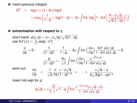
insert previous integral:

2F = logπ + (1−2α) log 2

+ extrq

11−q

+ log(1−q) + 2α∫

Dz log[1−Erf

( K−z√

q√2(1−q)

)]

extremisation with respect to q

short-hand u(z, q) = (κ−z√

q)/√

2(1−q),use Erf′(x) = 2√

πexp[−x2]

ddq

= 0 :1

(1−q)2 −1

1−q− 2α

∫Dz(∂u∂q

) Erf′ u(z, q)

1−Erf u(z, q)= 0

q(1−q)2 =

4α√π

∫Dz(∂u∂q

) e−u2(z,q)

1−Erf u(z, q)

work out: ∂u∂q

=1√2∂

∂qκ−z

√q

(1−q)1/2 = . . . =κ√

q − z2√

2q(1−q)3/2

insert into eqn for q:

q√

q = α

√2π

√1−q

∫Dz

e−u2(z,q)(κ√

q−z)

1−Erf u(z, q)


2F = logπ + (1−2α) log 2 +1

1−q+ log(1−q) + 2α

∫Dz log

[1−Erf u(z, q)

]q√

q = α

√2π

√1−q

∫Dz

e−u2(z,q)(κ√

q−z)

1−Erf u(z, q), u(z, q) =

κ−z√

q√2(1−q)

remember:F =finite: random data linearly separable with margin κF = −∞: random data not linearly separable with margin κ

α = 0 (so 1 N p):

q = 0, 2F = logπ + log 2 + 1 random data linearly separable (overfitting)

α > 0 (so 1 N ∼ p):

transition point: value of α where q → 1

1 = αc(κ)

√2π

∫Dz lim

q→1

√1−q

e−[ K−z√

2(1−q)]2

(κ−z)

1−Erf[

κ−z√2(1−q)

]αc(κ) =

[ 1√π

∫Dz (κ+z) lim

γ→∞

1γ

e−γ2(κ+z)2

1−Erf[γ(κ+z)]

]−1


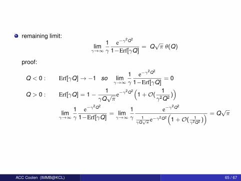
remaining limit:

limγ→∞

1γ

e−γ2Q2

1−Erf[γQ]= Q

√π θ(Q)

proof:

Q < 0 : Erf[γQ]→ −1 so limγ→∞

1γ

e−γ2Q2

1−Erf[γQ]= 0

Q > 0 : Erf[γQ] = 1− 1γQ√π

e−γ2Q2(

1 +O(1

γ2Q2 ))

limγ→∞

1γ

e−γ2Q2

1−Erf[γQ]= limγ→∞

1γ

e−γ2Q2

1γQ√π

e−γ2Q2(

1 +O( 1γ2Q2 )

) = Q√π


final result

αc(κ) =[ ∫ ∞−κ

Dz (κ+z)2]−1

αc(0) =[ ∫ ∞

0Dz z2

]−1= [

12

]−1 = 2

p covariates,N patients,binary outcomes,p and N large

random data(i.e. pure binary noise)is perfectly separable ifN/p < αc(κ)

algorithms (SVM etc)will find pars θ1 . . . θp

such that ti = sgn[∑pµ=1 θµx i

µ]for all i = 1 . . .N 0.0

0.5

1.0

1.5

2.0

0 1 2 3 4 5

classification margin κ

α = Np

αc(κ)

massiveoverfitting


part I of a short course on The replica method and its ...

Documents

Transcript of part I of a short course on The replica method and its ...