Part I Introduction and Course Overview - PKU · Part I Introduction and Course Overview Outline...

Digital Image Processing

Ming Jiang

May 19, 2010

Part I

Introduction and Course OverviewOutline

Contents

I Introduction and Course Overview 1

1 Digital image processing: What, Why and How 3

2 What Are the Difficulties 62.1 Poor understanding of human vision system . . . . . . . . . . . . . . . . . . . . . . . . . . 62.2 Internal representation is not directly understandable . . . . . . . . . . . . . . . . . . . . . 92.3 Why is computer vision difficult? . . . . . . . . . . . . . . . . . . . . . . . . . . . . . . . . 10

3 Image representation and image analysis tasks 12

4 Course Overview 17

II The Digitized Image and its Properties 18

5 Basic concepts 195.1 Image functions . . . . . . . . . . . . . . . . . . . . . . . . . . . . . . . . . . . . . . . . . . 195.2 Image formation . . . . . . . . . . . . . . . . . . . . . . . . . . . . . . . . . . . . . . . . . 205.3 Image as a stochastic process . . . . . . . . . . . . . . . . . . . . . . . . . . . . . . . . . . 22

6 Image digitization 226.1 Sampling . . . . . . . . . . . . . . . . . . . . . . . . . . . . . . . . . . . . . . . . . . . . . 236.2 Quantization . . . . . . . . . . . . . . . . . . . . . . . . . . . . . . . . . . . . . . . . . . . 26

7 Digital image properties 277.1 Metric and topological properties of digital images . . . . . . . . . . . . . . . . . . . . . . 28

7.1.1 Metric properties of digital images . . . . . . . . . . . . . . . . . . . . . . . . . . . 287.1.2 Topological properties of digital images . . . . . . . . . . . . . . . . . . . . . . . . 287.1.3 Contiguity paradoxes . . . . . . . . . . . . . . . . . . . . . . . . . . . . . . . . . . . 307.1.4 Other topological and geometrical properties . . . . . . . . . . . . . . . . . . . . . 32

7.2 Histogram . . . . . . . . . . . . . . . . . . . . . . . . . . . . . . . . . . . . . . . . . . . . . 347.3 Entropy . . . . . . . . . . . . . . . . . . . . . . . . . . . . . . . . . . . . . . . . . . . . . . 357.4 Visual perception of the image . . . . . . . . . . . . . . . . . . . . . . . . . . . . . . . . . 36

7.4.1 Contrast . . . . . . . . . . . . . . . . . . . . . . . . . . . . . . . . . . . . . . . . . . 367.4.2 Acuity . . . . . . . . . . . . . . . . . . . . . . . . . . . . . . . . . . . . . . . . . . . 37

1

7.4.3 Visual Illusions . . . . . . . . . . . . . . . . . . . . . . . . . . . . . . . . . . . . . . 377.5 Image quality . . . . . . . . . . . . . . . . . . . . . . . . . . . . . . . . . . . . . . . . . . . 387.6 Noise in images . . . . . . . . . . . . . . . . . . . . . . . . . . . . . . . . . . . . . . . . . . 40

7.6.1 Image Noise . . . . . . . . . . . . . . . . . . . . . . . . . . . . . . . . . . . . . . . . 407.6.2 Noise Type . . . . . . . . . . . . . . . . . . . . . . . . . . . . . . . . . . . . . . . . 417.6.3 Simulation of noise . . . . . . . . . . . . . . . . . . . . . . . . . . . . . . . . . . . . 417.6.4 The rejection method . . . . . . . . . . . . . . . . . . . . . . . . . . . . . . . . . . 437.6.5 The Polar method . . . . . . . . . . . . . . . . . . . . . . . . . . . . . . . . . . . . 457.6.6 Poissonian noise . . . . . . . . . . . . . . . . . . . . . . . . . . . . . . . . . . . . . 467.6.7 Mixed noise: Poissonian + Gaussian . . . . . . . . . . . . . . . . . . . . . . . . . . 46

8 Color Images 478.1 Physics of Color . . . . . . . . . . . . . . . . . . . . . . . . . . . . . . . . . . . . . . . . . 478.2 Color Perceived by Humans . . . . . . . . . . . . . . . . . . . . . . . . . . . . . . . . . . . 498.3 Color Spaces . . . . . . . . . . . . . . . . . . . . . . . . . . . . . . . . . . . . . . . . . . . 548.4 Palette Images . . . . . . . . . . . . . . . . . . . . . . . . . . . . . . . . . . . . . . . . . . 578.5 Color Constancy . . . . . . . . . . . . . . . . . . . . . . . . . . . . . . . . . . . . . . . . . 58

III Data structures for image analysis 58

9 Levels of Representation 59

10 Traditional Image Data Structures 6110.1 Matrices . . . . . . . . . . . . . . . . . . . . . . . . . . . . . . . . . . . . . . . . . . . . . . 6110.2 Chains . . . . . . . . . . . . . . . . . . . . . . . . . . . . . . . . . . . . . . . . . . . . . . . 6310.3 Topological Data Structures . . . . . . . . . . . . . . . . . . . . . . . . . . . . . . . . . . . 6410.4 Relational Structures . . . . . . . . . . . . . . . . . . . . . . . . . . . . . . . . . . . . . . . 65

11 Hierarchical Data Structures 6611.1 Pyramids . . . . . . . . . . . . . . . . . . . . . . . . . . . . . . . . . . . . . . . . . . . . . 6611.2 Quadtrees . . . . . . . . . . . . . . . . . . . . . . . . . . . . . . . . . . . . . . . . . . . . . 67

IV Image Pre-processing 68

12 Pixel Brightness Transformations 7012.1 Position dependent brightness correction . . . . . . . . . . . . . . . . . . . . . . . . . . . . 7012.2 Grey scale transformation . . . . . . . . . . . . . . . . . . . . . . . . . . . . . . . . . . . . 71

12.2.1 Windows and level . . . . . . . . . . . . . . . . . . . . . . . . . . . . . . . . . . . . 7412.2.2 Histogram stretching . . . . . . . . . . . . . . . . . . . . . . . . . . . . . . . . . . . 7512.2.3 Histogram Equalization . . . . . . . . . . . . . . . . . . . . . . . . . . . . . . . . . 7512.2.4 Histogram Matching . . . . . . . . . . . . . . . . . . . . . . . . . . . . . . . . . . . 77

13 Geometric Transformations 7813.1 Pixel Co-ordinate Transformations . . . . . . . . . . . . . . . . . . . . . . . . . . . . . . . 80

13.1.1 Polynomial Approximation . . . . . . . . . . . . . . . . . . . . . . . . . . . . . . . 8013.1.2 Bilinear Transformations . . . . . . . . . . . . . . . . . . . . . . . . . . . . . . . . 8013.1.3 Important Transformations . . . . . . . . . . . . . . . . . . . . . . . . . . . . . . . 81

13.2 Brightness Interpolation . . . . . . . . . . . . . . . . . . . . . . . . . . . . . . . . . . . . . 8113.2.1 Nearest Neighbor Interpolation . . . . . . . . . . . . . . . . . . . . . . . . . . . . . 8213.2.2 Bilinear Interpolation . . . . . . . . . . . . . . . . . . . . . . . . . . . . . . . . . . 8313.2.3 Bi-cubic interpolation . . . . . . . . . . . . . . . . . . . . . . . . . . . . . . . . . . 84

2

14 Local pre-processing 8514.1 Image smoothing . . . . . . . . . . . . . . . . . . . . . . . . . . . . . . . . . . . . . . . . . 86

14.1.1 Averaging . . . . . . . . . . . . . . . . . . . . . . . . . . . . . . . . . . . . . . . . . 8714.1.2 Averaging with Data Validity . . . . . . . . . . . . . . . . . . . . . . . . . . . . . . 8814.1.3 Averaging According to Inverse Gradient . . . . . . . . . . . . . . . . . . . . . . . 8814.1.4 Averaging Using a Rotating Mask . . . . . . . . . . . . . . . . . . . . . . . . . . . 8914.1.5 Median Filtering . . . . . . . . . . . . . . . . . . . . . . . . . . . . . . . . . . . . . 9014.1.6 Non-linear Mean Filtering . . . . . . . . . . . . . . . . . . . . . . . . . . . . . . . . 9214.1.7 Variational Properties of Smoothing Operators . . . . . . . . . . . . . . . . . . . . 93

14.2 Edge detectors . . . . . . . . . . . . . . . . . . . . . . . . . . . . . . . . . . . . . . . . . . 9414.2.1 Edge: what is it? . . . . . . . . . . . . . . . . . . . . . . . . . . . . . . . . . . . . . 9414.2.2 Finite Gradient . . . . . . . . . . . . . . . . . . . . . . . . . . . . . . . . . . . . . . 9614.2.3 More on Gradient Operators . . . . . . . . . . . . . . . . . . . . . . . . . . . . . . 9714.2.4 Roberts operator . . . . . . . . . . . . . . . . . . . . . . . . . . . . . . . . . . . . . 9814.2.5 Discrete Laplacian . . . . . . . . . . . . . . . . . . . . . . . . . . . . . . . . . . . . 9814.2.6 Prewitt Operator . . . . . . . . . . . . . . . . . . . . . . . . . . . . . . . . . . . . . 9914.2.7 Sobel Operator . . . . . . . . . . . . . . . . . . . . . . . . . . . . . . . . . . . . . . 9914.2.8 Robinson Operator . . . . . . . . . . . . . . . . . . . . . . . . . . . . . . . . . . . . 9914.2.9 Kirsch Operator . . . . . . . . . . . . . . . . . . . . . . . . . . . . . . . . . . . . . 9914.2.10 Image Sharpening . . . . . . . . . . . . . . . . . . . . . . . . . . . . . . . . . . . . 100

14.3 Zero-crossings of the Second Derivative . . . . . . . . . . . . . . . . . . . . . . . . . . . . . 10114.4 Scale in Image Processing . . . . . . . . . . . . . . . . . . . . . . . . . . . . . . . . . . . . 10414.5 Canny Edge Detection . . . . . . . . . . . . . . . . . . . . . . . . . . . . . . . . . . . . . . 10714.6 Parametric Edge Models . . . . . . . . . . . . . . . . . . . . . . . . . . . . . . . . . . . . . 11114.7 Edges in Multi-spectral Images . . . . . . . . . . . . . . . . . . . . . . . . . . . . . . . . . 11214.8 Line Detection by Local Pre-processing Operators . . . . . . . . . . . . . . . . . . . . . . 113

14.8.1 Line Detection . . . . . . . . . . . . . . . . . . . . . . . . . . . . . . . . . . . . . . 11314.8.2 Line Thinning . . . . . . . . . . . . . . . . . . . . . . . . . . . . . . . . . . . . . . 11414.8.3 Edge Filling . . . . . . . . . . . . . . . . . . . . . . . . . . . . . . . . . . . . . . . . 114

14.9 Detection of Corners (interesting points) . . . . . . . . . . . . . . . . . . . . . . . . . . . . 115

1 Digital image processing: What, Why and How

Vision

• Image is better than any other information form for our human being to perceive. Vision allowshumans to perceive and understand the world surrounding us.

• Human are primarily visual creatures. Not all animals depend on their eyes, as we do, for 99% or90% of the information received about the world [Russ, 1995, Zhao and Zhong, 1982].

Computer Vision

• Computer vision aims to duplicate the effect of human vision by electronically perceiving andunderstanding an image.

• Books other than this one would dwell at length on this sentence and the meaning of the wordduplicate

– whether computer vision is simulating or mimicking human systems is a philosophical territory,

– and one very fertile territory, too.

3

Figure 1: A frame from a video of a typical farmyard scene: the cow is one of a number walking naturallyfrom right to left.

3D vs 2D

• Giving computers the ability to see is not an easy task — we live in a three-dimensional (3D) world.

• When computers try to analyze objects in 3D space, the visual sensors available (e.g., TV cameras)usually give two-dimensional (2D) images.

• This projection from 3D to a lower number of dimensions incurs an enormous loss of information.

• Sometimes, equipment will deliver images that are 3D but this may be of questionable value:

– analyzing such datasets is clearly more complicated than 2D;

– sometimes the ’three-dimensionality’ is less than intuitive to us;

– terahertz scans are an example of this.

Video Analysis

• Dynamic scenes such as those to which we are accustomed, with moving objects or a moving camera,are increasingly common and represent another way of making computer vision more complicated.

Video Analysis: easy for human

• There are many reasons why we might wish to study scenes such as this, which are attractivelysimple to us

– the beast is moving slowly;

– it is clearly black and white;

– its movement is rhythmic.

• However, automated analysis is very fraught.

Video Analysis: difficult for computer

• The animal’s boundary is often very difficult to distinguish clearly from the background;

• the motion of the legs is self occluding;

• (subtly) the concept of cow-shaped is not something easily encoded.

4

Figure 2: Three frames from a cow sequence: notice the model can cope with partial occlusion as theanimal enters the scene, and the different poses exhibited.

Video Analysis: procedures

• The application from which this picture was taken made use of many of the algorithms presentedin this book:

– starting at a low level moving features were identified and grouped;

– a training phase taught the system what a cow might look like in various poses (see the figureon the right), from which a model of a moving cow could be estimated.

Various models for a cow silhouette: a straight-line boundary approximation has been learned from training

data and is able to adapt to different animals and different forms of occlusion.

Video Analysis: operations

• These models could then be fitted to new (unseen) video sequences.

• At this stage anomalous behavior such as lameness could be detected by the model failing to fitproperly, or well.

• Thus we see a sequence of operations

– image capture,

– early processing,

– segmentation,

– model fitting,

– motion prediction,

– qualitative and/or quantitative conclusion,

• that is characteristic of image understanding and computer vision problems.

Video Analysis: models and cow detection

5

Video Analysis: disscusions

• Each of these phases (which may not occur sequentially!) may be addressed by a number ofalgorithms which we shall cover in due course.

• The application was serious; there is a growing need in modern agriculture for automatic monitoringof animal health, for example to spot lameness.

• A limping cow is trivial for a human to identify, but it is very challenging to do this automatically.

Video Analysis: disscusions

• This example is relatively simple to explain, but serves to illustrate that many computer visiontechniques use the results and methods of

– mathematics,

– pattern recognition,

– artificial intelligence (AI),

– psycho-physiology,

– computer science,

– electronics,

– and other scientific disciplines.

2 What Are the Difficulties

Difficuties???

• Consider a single gray-scale (monochromatic) image, write down a few reasons why you feel auto-matic inspection and analysis of it may be difficult.

2.1 Poor understanding of human vision system

Human Vision

• How the human perceive process and store the visual information?

6

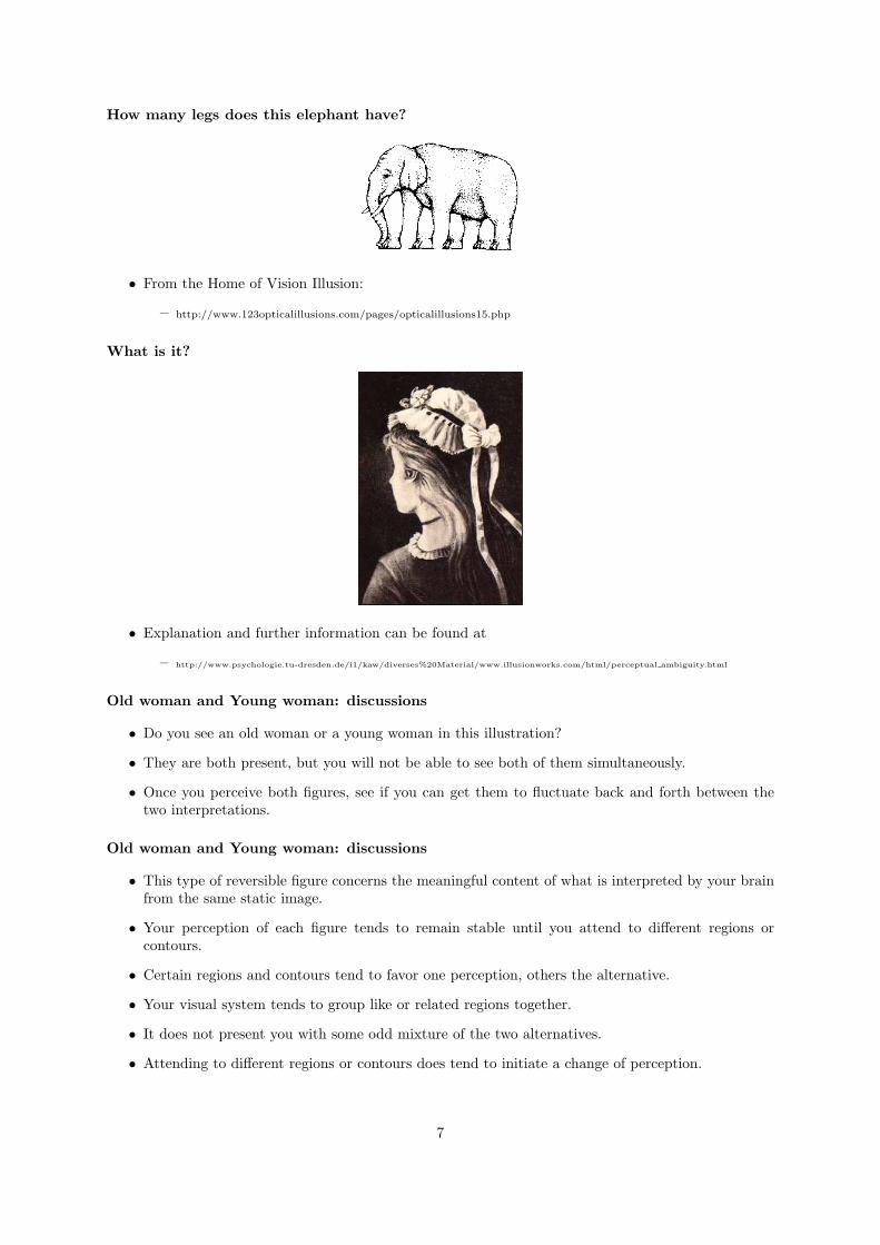
How many legs does this elephant have?

• From the Home of Vision Illusion:

– http://www.123opticalillusions.com/pages/opticalillusions15.php

What is it?

• Explanation and further information can be found at

– http://www.psychologie.tu-dresden.de/i1/kaw/diverses%20Material/www.illusionworks.com/html/perceptual ambiguity.html

Old woman and Young woman: discussions

• Do you see an old woman or a young woman in this illustration?

• They are both present, but you will not be able to see both of them simultaneously.

• Once you perceive both figures, see if you can get them to fluctuate back and forth between thetwo interpretations.

Old woman and Young woman: discussions

• This type of reversible figure concerns the meaningful content of what is interpreted by your brainfrom the same static image.

• Your perception of each figure tends to remain stable until you attend to different regions orcontours.

• Certain regions and contours tend to favor one perception, others the alternative.

• Your visual system tends to group like or related regions together.

• It does not present you with some odd mixture of the two alternatives.

• Attending to different regions or contours does tend to initiate a change of perception.

7

Human Vision

• We do not have a clear understanding how the human perceive, process and store the visualinformation.

• We do not even know how the human measures internally the image visual quality and discrimi-nation.

Perception ≡ Description

• If this image is looked at with a steady eye, it will still change, though less often.

• Researchers have stabilized the image directly onto the retina to eliminate any effects that mayarise from eye movements.

• Even under these conditions, a perceptual reversal may occur.

• This indicates that higher cortical processing occurs that strives to make meaning out of a stableimage presented to the retina.

• This illustrates once more that vision is an active process that attempts to make sense of incominginformation.

• As the late David Marr said, “Perception is the construction of a description.”

History of this illustration

• For many years the creator of this famous figure was thought to be British cartoonist W. E. Hill,who published it in 1915. Hill almost certainly adapted the figure from an original concept thatwas popular throughout the world on trading and puzzle cards.

• This anonymous dated German postcard (shown at the top of the page) from 1888 depicts theimage in its earliest known form.

The 1890 example on the left shows quite clearly its association as “My Wife and Mother-in-Law.” Both of these examples

predate the Punch cartoon that was previously thought to serve as the figure’s inspiration.


• The figure was later altered and adapted by others, including the two psychologists, R. W. Leeperand E. G. Boring who described the figure and made it famous within psychological circles in 1930.It has often been referred to as the “Boring figure.”

• Versions of the figure proved to be popular and the image was frequently reprinted; however, percep-tual biases started to occur in the image, unbeknownst to the plagiarizing artists and psychologistswho were reprinting the images.

• Variations have appeared in the literature that unintentionally are biased to favor one interpretationor another, which defeats its original purpose as a truly ambiguous figure.

8


• In the three versions shown above, can you tell which one is biased toward the young girl, the oldwoman?


• In 1961, J, Botwinick redesigned this figure once again, and entitled it, ”Husband and Father-in-Law.”

2.2 Internal representation is not directly understandable

Images as 2D functions

• Images are usually represented as a two dimensional function.

• Digitized images are usually represented by two dimensional array.

• However, those representations are not suitable for machine understanding, while the computer isable to process those representations.

• General knowledge, domain-specific knowledge, and information extracted from the image will beessential in attempting to understanding those arrays of numbers.

9

Experiment with images as 2D functions

• Read and display a image file as a two dimensional function.

• The example matlab script file is here matlab display example.

Images as 2D functions: discussions

• Both presentations contain exactly the same information.

• But for a human observer it is very difficult to find a correspondence between both.

• The point is that a lot of a priori knowledge is used by humans to interpret the images;

• the machine only begins with an array of numbers and so will be attempting to us more likely thefirst display than the second display.

2.3 Why is computer vision difficult?

Why is computer vision difficult?

• This philosophical question provides some insight into the rather complex landscape of computervision.

• It can be answered in many ways: we offer six.

• Here, we mention the reasons only briefly — most of them will be discussed in more detail later inthe book.

I. Loss of information

• Loss of information in projections from 3D to 2D is a phenomenon which occurs in typical imagecapture devices such as a camera or an eye.

• Their geometric properties have been approximated by a pinhole model for centuries (a box witha small hole in it, called in Latin a camera obscura [dark room]).

Pinhole camera

Figure 3: The pinhole model of imaging geometry does not distinguish size of objects.

• This physical model corresponds to a mathematical model of perspective projection.

• The projective transformation maps points along rays but does not preserve angles and collinearity.

10

II. Interpretation of images

• Interpretation of image(s) constitutes the principal tool of computer vision to approach problemswhich humans solve unwittingly.

• When a human tries to understand an image then previous knowledge and experience is broughtto the current observation.

• Human ability to reason allows representation of long-gathered knowledge, and its use to solve newproblems.

• Artificial intelligence has invested several decades in attempts to endow computers with the capa-bility to understand observations;

• while progress has been tremendous, the practical ability of a machine to understand observationsremains very limited.

• Attempting to solve related multidisciplinary scientific problems under the name cognitive systemsis seen as a key to developing intelligent machines.

Interpretation of images

• From the mathematical logic and/or linguistics point of view, interpretation of images can be seenas a mapping interpretation:

image data→ model (1)

• The (logical) model means some specific world in which the observed objects make sense.

• Examples

– nuclei of cells in a biological sample,

– rivers in a satellite image,

– or parts in an industrial process being checked for quality.

• There may be several interpretations of the same image(s).

Semantics of images

• Introducing interpretation to computer vision allows us to use concepts from mathematical logic,linguistics as syntax (rules describing correctly formed expression), and semantics (study of mean-ing).

• Considering observations (images) as an instance of formal expressions, semantics studies relationsbetween expressions and their meanings.

• The interpretation of image(s) in computer vision can be understood as an instance of semantics.

• Practically, if the image understanding algorithms know into which particular domain (model inlogical terminology) the observed world is constrained, then automatic analysis can be used forcomplicated problems.

III. Noise

• Noise is inherently present in each measurement in the real world.

• Its existence calls for mathematical tools which are able to cope with uncertainty; an example isprobability theory.

• Of course, more complex tools make the image analysis much more complicated compared tostandard (deterministic) methods.

11

IV. Too much data

• Images and video sequences are huge.

• An A4 sheet of paper scanned monochromatically at 300 dots per inch (dpi) at 8 bits per pixelcorresponds to 8.5 MB.

• Non-interlaced RGB 24 bit color video 512×768 pixels, 25 frames per second, makes a data streamof 225 Mb per second.

• If the processing we devise is not very simple, then it is hard to achieve real-time performance; i.e.,to process 25 or 30 images per second.

V. Complexity in mage formation

• Brightness measured in the image is given by complicated image formation physics.

• The radiance (brightness, image intensity) depends on the irradiance (light source type, in-tensity and position), the observer’s position, the surface local geometry, and the surface reflectanceproperties.

• The inverse tasks are ill-posed — for example, to reconstruct local surface orientation from intensityvariations.

VI. Local window vs. for global view

• Commonly, image analysis algorithms analyze a particular storage bin in an operational memory(e.g., a pixel in the image) and its local neighborhood;

• the computer sees the image through a keyhole.

• Seeing the world through a keyhole makes it very difficult to understand more global context.

• It is often very difficult to interpret an image if it is seen only locally or if only a few local keyholesare available.

Local parts of an image

Figure 4: Illustration of the world seen through several keyholes providing only a very local context.

The global view of the image

3 Image representation and image analysis tasks

Two Approaches

• There are philosophically two approaches: bionics and engineering (that is project attempt coor-dinated), approaches.

• The bionics approach has not been so successful, since we do have a through understanding aboutthe biological vision system.

12

Figure 5: How context is taken into account is an important facet of image analysis.

Image Understanding

• Image understanding by a machine can be seen as an attempt to find a relation between inputimage(s) and previously established models of the observed world.

• Transition from the input image(s) to the model reduces the information contained in the imageto relevant information for the application domain.

• This process is usually divided into several steps and several levels representing the image are used.

• The bottom layer contains raw image data and the higher levels interpret the data.

• Computer vision designs these intermediate representations and algorithms serving to establishand maintain relations between entities within and between layers.

Image Representation

• Image representation can be roughly divided according to data organization into four levels.

• The boundaries between individual levels arc inexact, and more detailed divisions are also proposed.

Image Representation & Hierarchy of Computer Vision

• This suggests a bottom up way of information processing, from signals with almost no abstraction,to the highly abstract description needed for image understanding.

• The flow of information does not need to be unidirectional.

• Feedback loops are often introduced to allow the modification of algorithms according to interme-diate results.

13

Two Levels

• This hierarchy of image representation and related algorithms is frequently categorized in an evensimpler way.

• Two levels are often distinguished:

– low-level image processing;

– high-level image understanding.

Low-level processing

• Low-level processing methods usually use very little knowledge about the content of images.

• Low-level methods often include image compression, pre-processing methods for noise filtering,edge extraction, and image sharpening.

• Ee shall discuss in this course.

• Low-level image processing uses data which resemble the input image.

• Very often, such a data set will be part of a video stream with an associated frame rate.

• E.g., an input image captured by a TV camera is 2D in nature, being described by an imagefunction f(x, y, t) whose value, at simplest, is usually brightness depending on parameters x, y andt.

High-level processing I

• High-level processing is based on knowledge, goals, and plans of how to achieve those goals.

• Artificial intelligence methods are widely applicable.

• High-level computer vision tries to imitate human cognition (although be mindful of the healthwarning given in the very first paragraph of this chapter) and the ability to make decisions accordingto the information contained in the image.

• In the example described, high-level knowledge would be related to the shape of a cow and thesubtle interrelationships between the different parts of that shape, and their (inter-)dynamics.

High-level processing II

• High-level vision begins with some form of formal model of the world, and then the “reality”perceived in the form of digitized images is compared to the model.

• A match is attempted.

• When differences emerge, partial matches (or sub-goals) are sought that overcome the mismatches.

• The omputer switches to low-level image processing to find information needed to update themodel.

• This process is then repeated iteratively, and “understanding” an image thereby becomes a co-operation between top-down and bottom-up processes.

• A feedback loop is introduced in which high-level partial results create tasks for low-level imageprocessing.

• The iterative image understanding process should eventually converge to the global goal.

14

Low- vs. high-level representations

• Both representations contain exactly the same information.

• But for a human observer it is not difficult to find a correspondence between them, and withoutthe second, it is unlikely that one would recognize the face of a child.

• The point is that a lot of a priori knowledge is used by humans to interpret the images.

• A machine only begins with an array of numbers and so will be attempting to make identificationsand draw conclusions from data that to us are more uncomprehensible.

• Increasingly, data capture equipment is providing very large data, sets that do not lend themselvesto straightforward interpretation by humans.

• We have already mentioned terahertz imaging as an example.

• General knowledge, domain-specific knowledge, and information extracted from the image will beessential in attempting to “understand” these arrays of numbers.

Low-level processingThe following sequence of processing steps is commonly recognized:

• Image Acquisition: An image is captured by a sensor (such as a TV camera) and digitized. Imagemay come in many formats and ways.

• Preprocessing: Image reconstruction or restoration, denoising and enhancement. E.g., computertomography.

• Image coding and compression: this is important for transferring images.

• Image segmentation: computer tries to separate objects from the image background.

• Object description and classification in a totally segmented image is also understood as part oflow-level image processing.

Image Segmentation

• Image segmentation is to separate objects from the image background and from each other.

• Total and partial segmentation may be distinguished.

• Total segmentation is possible only for very simple tasks, an example being the recognition ofdark non-touching objects from a light background.

• Example: optical character recognition, OCR.

• Een this superficially simple problem is very hard to solve without error.

• In more complicated problems (the general case), low-level image processing techniques handle thepartial segmentation tasks, in which only the cues which will aid further high-level processing areextracted.

• Often, finding parts of object boundaries is an example of low-level partial segmentation.

Low-level Image Processing

• Low-level computer vision techniques overlap almost completely with digital image processing,which has been practiced for decades.

• Object description and classification in a totally segmented image are also understood as part oflow-level image processing.

• Other low-level operations are image compression, and techniques to extract information from (butnot understand) moving scenes.

• .......

15

Low vs High

• Low-level image processing and high-level computer vision differ in the data used.

• Low-level data are comprised of original images represented by matrices composed of brightness(or similar) values.

• High-level data originate in images as well, but only those data which are relevant to high-levelgoals are extracted, reducing the data quantity considerably.

• High-level data represent knowledge about the image content. —

• E.g., object size, shape, and mutual relations between objects in the image.

• High-level data are usually expressed in symbolic form.

Image Processing

• Most current low-level image processing methods were proposed in the 1970s or earlier.

• Recent research is trying to find more efficient and more general algorithms, implementations.

• The requirement for better and faster algorithms is fuelled by technology delivering larger images(better spatial resolution), and color.

• A complicated and so far unsolved problem is how to order low-level steps to solve a specific task,and the aim of automating this problem has not yet been achieved.

• It is usually still a human operator who finds a sequence of relevant operations.

• Domain- specific knowledge and uncertainty cause much to depend on this operator’s intuition andprevious experience.

High-level Vision

• High-level vision tries to extract and order image processing steps using all available knowledge.

• Image understanding is the heart of the method, in which feedback from high-level to low-level isused.

• Unsurprisingly this task is very complicated and computationally intensive.

• David Marr’s book [Marr, 1982] influenced computer vision considerably throughout the 1980s.

• It described a new methodology and computational theory inspired by biological vision systems.

• Developments in the 1990s moved away from dependence on this paradigm, but interest in properlyunderstanding and then modeling human visual systems.

• It remains the case that the only known solution to the “vision problem” is our own brain!

3D Vision Problems

16

Figure 6: Several 3D vision tasks and algorithmic components expressed on different abstraction levels.We adopt the user’s view, i.e., what tasks performed routinely by humans would be good to accomplishby machines.

3D Vision Problems

• What is the relation of these 3D vision tasks to low-level (image processing) and high- level (imageanalysis) algorithmic methods?

• There is no widely accepted view in the academic community.

• Links between (algorithmic) components and representation levels are tailored to the specific ap-plication solved, e.g., navigation of an autonomous vehicle.

• These applications have to employ specific knowledge about the problem solved to be competitivewith tasks which humans solve.

• More general theories are expected to emerge.

• Many researchers in different fields work on related problems.

• There is a belief that research in ’cognitive systems’ could be the key.

4 Course Overview

Course Overview

• Digital image processing, image analysis, image understanding are related branches of computervision.

• This course is about digital image processing.

• The following topics are to be covered in this course.

Course Syllabus

• Introduction and Course Overview

• Image representations and properties

– Images as a stochastic processes or linear systems, etc.

– Metric and topological properties of digital images

– Histograms

– Noise in images

• Data Structures for Image Analysis

17

• Image Pre-processing

– Various pre-processing operators

• Image Segmentation

– Thresholding, edge-based, region growing, segmentation method.

• Scale Space Theory

– Image processing and partial differential equations.

The textbook and web resource

• Milan Sonka, V. Hlavac, R. Boyle: Image Processing, Analysis and Machine Vision, 3rd edition.Thomson Learning, 2008.

• Image Processing, Analysis, and Machine Vision: A MATLAB Companion, http://visionbook.felk.cvut.cz/

References

• Kenneth R. Castleman: Digital Image Processing. Prentice-Hall International, Inc. 1996. OrTsinghua University Press, 1998.

• Rongchun Zhao: Introduction to Digital Image Processing (in Chinese). Northwestern Polytechni-cal University Press, 2000.

Summary

• Human vision is natural and seems easy; computer mimicry of this is difficult.

• We might hope to examine pictures, or sequences of pictures, for quantitative and qualitativeanalysis.

• Many standard and advanced AI techniques are relevant.

• “High” and “low” levels of computer vision can be identified.

• Processing moves from digital manipulation, through pre-processing, segmentation, and recognitionto understanding — but these processes may be simultaneous and co-operative.

• An understanding of the notions of heuristics, a priori knowledge, syntax, and semantics is neces-sary.

• The vision literature is large and growing; books may be specialized, elementary, or advanced.

• A knowledge of the research literature is necessary to stay up to date with the topic.

• Developments in electronic publishing and the Internet are making access to vision simpler.

Part II

The Digitized Image and its PropertiesOutline

Contents

18

5 Basic concepts

Signals

• Fundamental concepts and mathematical tools are introduced in this chapter which will be usedthroughout the course.

• Mathematical models are often used to describe images and other signals.

• A signal is a function depending on some variable(s) with physical meaning. Signals can be

– one-dimensional (e.g., audio signal dependent on time);– two-dimensional (e.g., images dependent on two co-ordinates in a plane);– three-dimensional (e.g., describing an object in space or video signal);– or higher-dimensional.


• A scalar function may be sufficient to describe a monochromatic image.

• Vector functions are to represent, for example, color images consisting of three component colors.

• Functions we shall work with may be categorized as continuous, discrete and digital.

• A continuous function has continuous domain and range;

• If the domain set is discrete, then we get a discrete function;

• if the range set is also discrete, then we have a digital function.

5.1 Image functions


• An image can be modeled by a continuous function of two or three variables;

• Its arguments are co-ordinates x and y in a plane;

• If images change in time a third variable t might be added.

• The image function values correspond to the brightness at image points.

Intepretation of image values

• The function value can express other physical quantities as well (temperature, pressure distribution,distance from the observer, etc.).

• The brightness integrates different optical quantities — using brightness as a basic quantity allowsus to avoid the description of the very complicated process of image formation.

HomeworkDiscuss the various factors that influence the brightness of a pixel in an image.

2D images

• The image on the human eye retina or on a TV camera sensor is intrinsically 2D.

• We shall call such a 2D image bearing information about brightness points an intensity image.

• The real world which surrounds us is intrinsically 3D.

• The 2D intensity image is the result of a perspective projection of the 3D scene.

19

Ill-posed problem I

• When 3D objects are mapped into the camera plane by perspective projection a lot of informationdisappears as such a transformation is not one-to-one.

• Recognizing or reconstructing objects in a 3D scene from one image is an ill-posed problem.

• Recovering information lost by perspective projection is only one, mainly geometric, problem ofcomputer vision.

• The aim is to recover a full 3D representation such as may be used in computer graphics.

Ill-posed problem II

• The second problem is how to understand image brightness.

• The only information available in an intensity image is the brightness of pixels.

• They are dependent on a number of independent factors such as

– object surface reflectance properties (given by the surface material, micro-structure and mark-ing),

– illumination properties,

– object surface orientation with respect to a viewer and light source.

• This is a non-trivial and again ill-posed problem.

2D or 3D

• Some applications work with 2D images directly; for example,

– an image of the flat specimen viewed by a microscope with transparent illumination;

– a character drawn on a sheet of paper;

– the image of a fingerprint, etc.

• Many basic and useful methods used in digital image analysis do not depend on whether the objectwas originally 2D or 3D (e.g, FFT).

5.2 Image formation

Image formation: I

• The image formation process is described in [Horn, 1986, Wang and Wu, 1991].

• Related disciplines are photometry which is concerned with brightness measurement, and colorime-try which studies light reflectance or emission depending on wavelength.

Image formation: II

• A light source energy distribution C(x, y, t, λ) depends in general on image co-ordinates (x, y), timet, and wavelength λ.

• For the human eye and most technical image sensors (e.g., TV cameras), the “brightness” f dependson the light source energy distribution C and the spectral sensitivity of the sensor, S(λ) (dependenton the wavelength)

f(x, y, t) =∫ ∞

0

C(x, y, t, λ)S(λ) dλ (2)

• An intensity image f(x, y, t) provides the brightness distribution.

20

Multi-spetral images

• In a color or multi-spectral image, the image is represented by a real vector function f

f(x, y, t) = (f1(x, y, t), f2(x, y, t), · · · , fn(x, y, t)) (3)

where, for example, there may be red, green and blue, three components.

Monochromatic static image

• Image processing often deals with static images, in which time t is constant.

• A monochromatic static image is represented by a continuous image function f(x, y) whose argu-ments are two co-ordinates in the plane.

• Most methods introduced in this course is primarily for intensity static image.

• It is often the case that the extension of the techniques to the multi-spectral case is obvious.

Monochromatic static image

• Computerized image processing uses digital image functions which are usually represented by ma-trices.

• Co-ordinates are integer numbers.

• The domain of the image function is a region R in the plane

R = {(x, y) : 1 ≤ x ≤ xm, 1 ≤ y ≤ yn} (4)

where xm and yn represent maximal image co-ordinates.

Limited domain

• The image function has a limited domain — infinite summation or integration limits can be used,as it is assumed that the image function is zero outside the domain.

• The customary orientation of co-ordinates in an image is in the normal Cartesian fashion (horizontalx axis, vertical y axis).

• The (row, column) orientation used in matrices is also quite often used in digital image processing.

Limited range

• The range of image function values is also limited; by convention, in intensity images the lowestvalue corresponds to black and the highest to white.

• Brightness values bounded by these limits are gray levels.

• The gray level range is 0, 1, · · · , 255, represented by 8 bits, the data type used is unsigned char.In some applications, 14 bits or more is used, e.g, for medical images.

• The usual computer display supports 8 bit gray level.

Homework

• How to display a 16 bit gray level image? Generate an image of 16 bit and try to display it withyour computer.

• If a discrete image is of continuous range, the image matrix is of type float or double. How todisplay it? Generate an image of float or double type and try to display it with your computer.

21

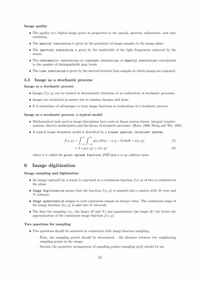
Image quality

• The quality of a digital image grows in proportion to the spatial, spectral, radiometric, and timeresolution.

• The spatial resolution is given by the proximity of image samples in the image plane.

• The spectral resolution is given by the bandwidth of the light frequencies captured by thesensor.

• The radiometric resolution (or contrast resolution, or density resolution) correspondsto the number of distinguishable gray levels.

• The time resolution is given by the interval between time samples at which images are captured.

5.3 Image as a stochastic process

Image as a stochastic process

• Images f(x, y) can be treated as deterministic functions or as realizations of stochastic processes.

• Images are statistical in nature due to random changes and noise.

• It is sometimes of advantages to treat image functions as realizations of a stochastic process.

Image as a stochastic process: a typical model

• Mathematical tools used in image description have roots in linear system theory, integral transfor-mations, discrete mathematics and the theory of stochastic processes, [Horn, 1986, Wang and Wu, 1991].

• A typical image formation model is described by a linear spatial invariant system,

f(x, y) =∫ ∞−∞

∫ ∞−∞

g(a, b)h(x− a, y − b) dadb+ n(x, y) (5)

= h ∗ g(x, y) + n(x, y) (6)

where h is called the point spread function (PSF)and n is an additive noise.

6 Image digitization

Image sampling and digitization

• An image captured by a sensor is expressed as a continuous function f(x, y) of two co-ordinates inthe plane.

• Image digitization means that the function f(x, y) is sampled into a matrix with M rows andN columns.

• Image quantization assigns to each continuous sample an integer value. The continuous range ofthe image function f(x, y) is split into K intervals.

• The finer the sampling (i.e., the larger M and N) and quantization (the larger K) the better theapproximation of the continuous image function f(x, y).

Two questions for sampling

• Two questions should be answered in connection with image function sampling:

– First, the sampling period should be determined – the distance between two neighboringsampling points in the image;

– Second, the geometric arrangement of sampling points (sampling grid) should be set.

22

6.1 Sampling

Sampling intervals

• A continuous image function f(x, y) can be sampled using a discrete grid of sampling points in theplane.

• The image is sampled at points x = j∆x, y = k∆y

• Two neighboring sampling points are separated by distances ∆x along the x axis and ∆y alongthe y axis.

• Distances ∆x and ∆y are called the sampling interval.

• The matrix of samples constitutes the discrete image.

Sampled Image

• The ideal sampling s(x, y) in the regular grid can be represented using a collection of Dirac distri-butions

s(x, y) =∞∑

j=−∞

∞∑k=−∞

δ(x− j∆x, y − k∆y) (7)

• The sampled image is the product of the continuous image f(x, y) and the sampling function s(x, y)

fs(x, y) = s(x, y)f(x, y) (8)

Sampled Image

• The collection of Dirac distributions in equation (7) can be regarded as periodic with period ∆x,∆y.

• It can be expanded into a Fourier series (assuming for a moment that the sampling grid covers thewhole plane (infinite limits))

s =∞∑

m=−∞

∞∑n=−∞

amne2πi(mx∆x+ ny∆y ) (9)

Fourier expansion

• The coefficients of the Fourier expansion can be calculated as

amn =1

∆x∆y

∫ ∆x2

−∆x2

∫ ∆y2

−∆y2

∞∑j=−∞

∞∑k=−∞

δ(x− j∆x, y − k∆y)e2πi(mx∆x+ ny∆y ) dxdy (10)

• Noting that only the term for j = 0 and k = 0 in the sum is nonzero in the range of integration(for other j and k, the center of the Delta function is outside the integral interval), the coefficientsare

amn =1

∆x∆y(11)

23

Fourier expansion in the frequency domain

• Then, (8) can be rewritten as

fs(x, y) = f(x, y)1

∆x∆y

∞∑m=−∞

∞∑n=−∞

e2πi(mx∆x+ ny∆y ) (12)

• In the frequency domain then

Fs(u, v) =1

∆x∆y

∞∑m=−∞

∞∑n=−∞

F (u− m

∆x, v − n

∆y) (13)

where F and Fs are the Fourier transform of f and fs respectively.

Fourier transform of the sampled image

• Recall the Fourier transform is

F (u, v) =∫ ∞−∞

∫ ∞−∞

f(x, y)e−2πi(ux+vy) dxdy (14)

• Thus the Fourier transform of the sampled image is the sum of periodically repeated Fouriertransforms F (u, v) of the origin image.

• Periodic repetition of the Fourier transform result F (u, v) may under certain conditions causedistortion of the image which is called aliasing.

• This happens when individual digitized components F (u, v) overlap.

Aliasing

• There is no aliasing if the image function f(x, y) has a band limited spectrum, its Fourier transformF (u, v) = 0 outside a certain interval of frequencies |u| > U and |v| > V .

T-U-U U T

Figure 7: Where T = 1∆x .

Shannon sampling theorem

• From general sampling theory [Oppenheim et al., 1997], aliasing can be prevented if the samplinginterval is chosen according to

∆x ≤ 12U

, ∆x ≤ 12V

. (15)

• This is the Shannon sampling theorem that has a simple physical interpretation in image analysis

– the sampling interval should be chosen such that it is less than or equal to half of the smallestinteresting detail in the image.

24

Sampling function in practice

• The sampling function is not the Dirac distribution in real digitizers – narrow impulses with limitedamplitude are used instead.

• Assume a rectangular sampling grid which consists of M × N such equal and non-overlappingimpulses hs(x, y) with sampling period ∆x and ∆y.

• Ideally, hs(x, y) = δ(x, y).

• The function hs(x, y) simulates realistically the real image sensors.

• Outside the sensitive area of the sensor, the sampling element hs(x, y) = 0.

Sampled image in practice

• The sampled image is then given by the following convolution

fs(x, y) = f(x, y)∞∑

j=−∞

∞∑k=−∞

hs(x− j∆x, y − k∆y) (16)

• The sampled image fs is distorted by the convolution of the original image f and the limitedimpulse hs.

• The distortion of the frequency spectrum of the function Fs can be expressed as follows

Fs(u, v) =1

∆x∆y∞∑

m=−∞

∞∑n=−∞

F (u− m

∆x, v − n

∆y)Hs(

m

∆x,n

∆y). (17)

Homework

• Prove Eq. (17) from Eq. (16).

Homework

• There are other sampling schemes.

• These sampling points are ordered in the plane and their geometric relation is called the grid.

• Grids used in practice are mainly square or hexagonal

25

Pixels

• One infinitely small sampling point in the grid corresponds to one picture element (pixel) in thedigital image.

• The set of pixels together covers the entire image.

• Pixels captured by a real digitization device have finite sizes.

• A pixel is a unit which is not further divisible.

• Sometimes pixels are also called points.

Real digitizers

• In real image digitizers, a sampling interval about ten times smaller than that indicated by theShannon sampling theorem (15) is used.

• This is because algorithms which reconstruct the continuous image on a display from the digitizedimage function use only a step function.

• E.g., a line in the image is created from pixels represented by individual squares.

• The situation is more complicated.

• Average sampling happens in practice.

Sampling Examples

Figure 8: Digitizing, (a) 256× 256. (b) 128× 128. (c) 64× 64. (d) 32× 32. Images have been enlargedto the same size to illustrate the loss of detail.

6.2 Quantization

Quantization

• The magnitude of a sampled image is expressed as a digital value in image processing.

• The transition between continuous values of the image function (brightness) and its digital equiv-alent is called quantization.

• The number of quantization levels should be high enough for human perception of fine shadingdetails in the image.

26

False Contours in Images

• The occurrence of false contours is the main problem in image which have been quantized withinsufficient brightness levels.

• This effect arises when the number of brightness levels is lower than that which humans can easilydistinguish.

False Contours in Color Images

Discussions on Quantization

• This number is dependent on many factors: e.g., the average local brightness.

• Displays which avoids this effect will normally provide a range of at least 100 intensity levels.

• This problem can be reduced when quantization into intervals of unequal length is used.

• The size of intervals corresponding to less probable brightnesses in the image is enlarged.

• These gray-scale transformation techniques are considered in later sections.

• Most digital image processing devices use quantization into k equal intervals.

• If b bits are used ... the number of brightness levels is k = 2b.

• Eight bits per pixel are commonly used, specialized measuring devices use 12 and more bits perpixel.

Quantization Experiment with matlabDo you observe false contours when the quantization levels is decreasing?

7 Digital image properties

Digital Properties

• A digital image has several properties,...

• both metric and topological,

• which are somewhat different from those of continuous two-dimensional functions we are familiarwith.

27

7.1 Metric and topological properties of digital images

Continuous Property May not Hold

• A digital image consists of picture elements of finite size.

• Usually pixels are arranged in a rectangular grid.

• A digital image is represented by a two-dimensional matrix whose elements are integer numberscorresponding to the quantization levels in the brightness scale.

• Some intuitively clear properties of continuous images have no straightforward analogy in thedomain of digital images.

7.1.1 Metric properties of digital images

Distance

• Distance is an important example.

• The distance between two pixels in a digital image is a significant quantitative measure.

• The distance between points with co-ordinates (i, j) and (h, k) may be defined in several differentways.

Euclidean Distance

• The Euclidean distance DE is defined by

DE [(i, j), h, k] =√

(i− h)2 + (j − k)2 (18)

• The advantage of the Euclidean distance is the fact that it is intuitively obvious.

• The disadvantages are costly calculation due to the square root, and its not-integer value.

TAXI Distance

• The distance between two points can also expressed as the minimum number of elementary stepsin the digital grid which are needed to move from the starting point to the end point.

• If only horizontal and vertical moves are allowed, the distance D4 or city block distance is obtained:

D4[(i, j), h, k] = |i− h|+ |j − k| (19)

• This is the analogy with the distance between two locations in a city with a rectangular grid ofstreets and closed blocks of buildings.

Chess-board Distance

• If moves in diagonal directions are allowed in addition, the distance D8 or the chess-board distanceis obtained:

D8[(i, j), h, k] = max{|i− h|, |j − k|} (20)

7.1.2 Topological properties of digital images

Pixel Neighborhoods

• Pixel adjacency is another important concept in digital images.

• Any two pixels are called 4-neighbors if they have distance D4 = 1 from each other.

• 8-neighbors are two pixels with D8 = 1.

• 4-neighbors and 8-neighbors are illustrated in Figure 111.

28

Figure 9: Pixel neighborhoods.

Regions and Paths

• It will become necessary to consider important sets consisting of several adjacent pixels — regions.

• Region is a contiguous (touching, neighboring, near to) set.

• A path from pixel P to pixel Q as a sequence of points A1, A2, · · · , An, where A1 = P and An = Q,and Ai+1 is a neighbor of Ai, i = 1, · · · , n− 1.

• A region is a set of pixels in which there is a path between any pair of its pixels, all of whosepixels also belong to the set.

Contiguity

• If there is a path between two pixels in the set of pixels in the image, these pixels are calledcontiguous.

• The relation to be contiguous is reflexive, symmetric and transitive and therefore defines a decom-position of the set (in our case image) into equivalence classes (regions).

• The following image illustrates a binary image decomposed by the relation contiguous into threeregions.

Some Terms

• Assume that Ri are disjoint regions in the image and that these regions do not touch the imageboundary (to avoid special cases).

• Let R be the union of all regions Ri. Let RC be the complement of R with respect to the image.

• The subset of RC , which is contiguous with the image boundary, is called background, and therest of the complement RC is called holes.

• If there are no holes in a region we call it a simply contiguous region.

• A region with holes is called multiply contiguous.

29

Image Segmentation

• Note that the concept of region uses only the property to be contiguous.

• Secondary properties can be attached to regions which originate in image data interpretation.

• It is common to call some regions in the image objects.

• A process which determines which regions in an image correspond to objects in the world is partof image segmentation.

Contiguous Example

• The brightness of a pixel is a property used to find objects in some images.

• If a pixel is darker than some other predefined values (threshold), then it belongs to some object.

• All such points which are also contiguous constitute one object.

• A hole consists of points which do not belong to the object and surrounded by the object, and allother points constitute the background.

• An example is the black printed text on the white paper, in which individual letters are objects.

• White areas surrounded by the letter are holes, e.g., the area inside a letter ’O’.

• Other parts of the paper are background.

7.1.3 Contiguity paradoxes

Contiguity paradoxes

• These neighborhood and contiguity definitions on the square grid create some paradoxes.

Line Contiguous ParadoxThe following figure shows three digital lines with 45o and −45o slope.

• If 4-connectivity is used, the lines are not contiguous at each of their points.

• An even worse conflict with intuitive understanding of line properties is:

– two perpendicular lines do intersect in one case (upper right intersection) and do not intersectin another case (lower left), as they do not have any common point.

30

Jordon Paradox

• Each closed curve divides the plane into two non-contiguous regions.

• If image are digitized in a square grid using 8-connectivity, there is a line from the inner part of aclosed curve into the outer part without intersecting the curve.

• This implies that the inner and outer parts of the curve constitute one contiguous region.

Connectivity paradox

• If we assume 4-connectivity, the figure contains four separate contiguous regions A, B, C and D.

– A ∪B are disconnected, as well as C ∪D.

– A topological contradiction.

– Intuitively, C ∪D should be connected if A ∪B are disconnected.

Connectivity paradox

• If we assume 8-connectivity, there are two regions, A ∪B and C ∪D.

• Both sets contain paths AB and CD entirely within themselves, but which also intersect!

31

Ad Hoc Solutions to Paradoxes

• One possible solution to contiguity paradox is to treat objects using 4-neighborhoods and back-ground using 8-neighborhoods (or vice versa).

• More exact treatment of digital contiguity paradox and their solution for binary images and imageswith more brightness levels can be found in [Pavlidis, 1977].

• These problems are typical on square grids — a hexagonal grid (96) solves many of them.

• However, a grid of this type has also a number of disadvantages, [Pavlidis, 1977], p. 60.

• For reasons of simplicity and ease of processing, most digitizing devices use a square grid despitethe stated drawbacks.

• We do not pursue further into this topic in this course, but use the simple approach, although thereare some paradoxes.

Solutions to Paradoxes

• An alternative approach to the connectivity problems is to use discrete topology based on CWcomplex theory in topology.

• It is called cell complex in [Kovalevski, 1989].

• This approach develops a complete strand of image encoding and segmentation.

• The idea, first proposed by Riemann in the nineteenth century, considers families of sets of differentdimensions:

– points, which are 0-dimensional, may then be assigned to sets containing higher dimensionalstructures (such as pixel array), which permits the removal of the paradoxes we have seen.

– line segments, which are 1-dimensional, gives precise definition of edge and border.

7.1.4 Other topological and geometrical properties

Border

• Border of a region is another important concept in image analysis.

• The border of a region R is the set of pixels within the region that have one or more neighborsoutside R.

• This definition of border is sometimes referred to as inner border, to distinguish it from the outerborder,

– it is the border of the background (i.e., the complement of) of the region.

Edge

• Edge is a local property of a pixel and its immediate neighborhood — it is a vector given by amagnitude and direction.

• The edge direction is perpendicular to the gradient direction which points in the direction of imagefunction growth.

32

Border and Edge

• The border is a global concept related to a region, while edge expresses local properties of an imagefunction.

• The border and edge are related as well.

• One possibility for finding boundaries is chaining the significant edges (points with high gradientof the image function).

Crack Edge I

• The edge property is attached to one pixel and its neighborhood.

• It is of advantage to assess properties between pairs of neighboring pixels.

• The concept of the crack edge comes from this idea.

Crack Edge II

• Four crack edges are attached to each pixel, which are defined by its relation to its 4-neighbors.

• The direction of the crack edge is that of increasing brightness, and is a multiple of 90 degrees.

• Its magnitude is the absolute difference between the brightness of the relevant pair of pixels.

Convex Hull

• Convex hull is used to describe geometrical properties of objects.

• The convex hull is the smallest convex region which contains the object,

– such that any two points of the region can be connected by a straight line, all points of whichbelong to the region.

Lakes and Bays

• An object can be represented by a collection of its topological components.

• The sets inside the convex hull which does not belong to an object is called the deficit of convexity.

• This can be split into two subsets.

1. lakes are fully surrounded by the objects.

2. bays are contiguous with the border of the convex hull of the object.

• The convex hull, lakes and bays are sometimes used for object description.

33

7.2 Histogram

Brightness Histogram

• Brightness histogram provides the frequency of the brightness value in the image.

• The brightness histogram hf (z) is a function showing,

– for each brightness value z,

– the number of pixels in the image f that have that brightness value z.

Computing Brightness Histogram

• The histogram of an image with L gray levels is represented by a one-dimensional array with Lelements.

• For a digital image of brightness value ranging in [0, L − 1], the following algorithm produces thebrightness histogram:

1. Assign zero values to all element of the array hf ;

2. For all pixels (x, y) of the image f , increment hf [f(x, y)] by 1.

Brightness Histogram Example

• The histogram is often displayed as a bar graph.

Computation Options

• Computing brightness histogram is similar to generating the histogram of a random variable froma given group of samples.

• In the above algorithm, the starting value is 0, bin-width 1, and bin number L.

• This algorithm can be modified to generate brightness histogram of arbitrary bin-width and binnumber.

• For multi-spectral band images, histogram of each individual band can be generated in a similarway.

34

Brightness Histogram Example: non-convential bin

Histogram: discussions I

• The histogram provides a natural bridge between images and a probabilistic description.

• Wc might want to find a first-order probability function pI(z;x, y) to indicate the probability thatpixel (x, y) has brightness z.

• Dependence on the position of the pixel is not of interest in the histogram.

Histogram: discussions II

• The histogram is usually the only global information about the image which is available.

• It is used when finding optimal illumination conditions for capturing an image, gray-scale trans-formations, and image segmentation to objects and background.

• Note that one histogram may correspond to several images;

– e.g., a change of the object position on a constant background does not affect the histogram.

Histogram: discussions II

• The histogram of a digital image typically has many local minima and maxima, which may com-plicate its further processing.

• This problem can be avoided by local smoothing of the histogram.

• This algorithm would need some boundary adjustment, and carries no guarantee of removing alllocal minima.

• Other techniques for smoothing exist, notably Gaussian blurring.

Histogram Experiment with matlab

• Creating an image histogram using imhist.

7.3 Entropy

Entropy

• Image information content can be estimated using entropy H.

• The concept of entropy has roots in thermodynamics and statistical mechanics, but it took manyyears before entropy was related to information.

• The information-theoretic formulation of entropy comes from Shannon [Shannon, 1948] and is oftencalled information entropy.

35

Entropy As a Measure of uncertainty

• An intuitive understanding of information entropy relates to the amount of uncertainty about anevent associated with a given probability distribution.

• The entropy can serve as an measure of “disorder”.

• As the level of disorder rises, entropy increases and events are less predictable.

Entropy: definition

• The entropy is defined formally assuming a discrete random variable X with possible outcomes(called also states) x1, · · · , xn.

• Let p(xk) be the probability of the outcome xk, k = 1, · · · , n.

• Then the entropy is defined as

H(x) =n∑k=1

p(xk) log1

p(xk)= −

n∑k=1

p(xk) log p(xk). (21)

• log 1p(xk) is called the surprisal of the outcome xk.

• The entropy is the expected value of its outcome’s surprisal.

Entropy: discussions

• The base of the logarithm in this formula determines the unit in which entropy is measured.

• If this base is two then the entropy is given in bits.

• The entropy is often estimated using a gray-level histogram in image analysis.

• Because entropy measures the uncertainty about the realization of a random variable, it is used toassess redundancy in an image for image compression.

7.4 Visual perception of the image

Visual Perception

• Anyone who creates or uses algorithms or devices for digital image processing should take intoaccount the principle of human visual perception.

• There are psycho-physical parameters such as contrast, border, shape, texture, color, etc.

• Humans will find objects in images only if they may be distinguished effortlessly from the back-ground.

• Human perception of image provokes many illusions, the understanding of which provides valuableclues about visual mechanisms.

• The topic is covered exhaustively from the point of view of computer vision in [Frisby, 1979].

7.4.1 Contrast

Contrast

• Contrast is the local change in brightness and is defined as the ratio between average brightness ofan object and the background brightness.

• The human eye is logarithmically sensitive to brightness.

• Gamma correction is used to calibrate the differences among different computer monitors.

• Apparent brightness depends very much on the brightness of the local background; this effect iscalled conditional contrast.

36

Conditional Contrast

• The figure illustrates this effect with two small squares of the same brightness on a dark and alight background.

• Human perceives the brightness of the small squares as different.

7.4.2 Acuity

Acuity

• Acuity is the ability to detect details in image.

• The human eye is less sensitive to slow and fast brightness changes but is more sensitive to inter-mediate changes.

• Resolution in an image is firmly bounded by the resolution ability of the human eye;

• there is no sense in representing visual information with higher resolution than that of the viewer.

Resolution

• Resolution in optics is defined as the inverse value of a maximum viewing angle between the viewerand two proximate points which human cannot distinguish, and so fuse together.

• Human vision has the best resolution for objects which are at a distance of about 25 cm from aneye under illumination of about 500 lux.

• This illumination is provided by a 60 W from a distance 40 cm.

• Under this conditions the distance between two distinguishable points is approximately 0.16 mm.

• Another report says that the minimal distinguishable distance is 0.47 mm [Kutter, 1999].

QuizGiven the above two minimal distinguishable distance, what is the resolution in DPI needed for a

printer to produce perfect output?DPI means “Dots Per Inch” (1 in = 2.54 cm).

7.4.3 Visual Illusions

Visual Illusions

• Human perception of images is prone to many illusions.

• There are many other visual illusions caused by phenomena such as color or motion;

• an Internet search will produce examples easily.

37

The Ebbinghaus Circles

• Object borders carry a lot of information.

• Boundaries of objects and simple patterns such as blobs or lines enable adaption effects similar toconditional contrast.

• The Ebbinghaus illusion is a well known example — two circles of the same diameter in the centerof images appear to have different sizes.

Parallel Lines

• Perception of one dominant shape can be fooled by nearby shapes.

• This figure shows parallel diagonal line segments which are not perceived as parallel.

Zigzag Lines

• This figure contains rows of black and white squares which are all parallel.

• However, the vertical zigzag squares disrupt our horizontal perception.

7.5 Image quality

Image Quality

• An image might be degraded during capture, transmission, or processing.

38

• Measures of image quality can be used to assess the degree of degradation.

• The quality required naturally depends on the purpose for which an image is used.

• Methods for assessing image quality can be divided into two categories: subjective and objective.

Subjective Quality

• Subjective methods are often used in television technology.

• The ultimate criterion is the perception of a selected group of professional and lay viewers.

• They appraise an image according to a list of criteria and give appropriate marks.

Objective Quality

• Objective quantitative methods measuring image quality are more interesting for our purposes.

• Ideally such a method also provides a good subjective test, and is easy to apply;

• we might then use it as a criterion in parameter optimization.

Image Quality: MSE, etc.

• The quality of the image f(x, y) is usually estimated by comparison with a known reference imageg(x, y).

• A synthesized image g(x, y) is often used for this purpose.

• One class of methods uses simple measures such as the mean quadratic difference (or mean squarederror, MSE)

MSE(g, f) =1N

∑x,y

(g(x, y)− f(x, y))2 (22)

where N is the number of pixels.

• The problem here is that it is not possible to distinguish a few big differences from a lot of smalldifferences.

• Instead of the mean quadratic difference, the mean absolute difference or simply maximal absolutedifference may be used.

• Correlation between images f and g is another alternative.

Image Quality: SNR

• Signal to noise ratio SNR is also used as a image degradation measure.

• Let f(x, y) be the original image and f ′(x, y) be the degraded image, the degree of degradation ismeasured by

SNR(f ′, f) = 10 log10

∑x,y f(x, y)2∑

x,y(f(x, y)− f ′(x, y))2(db) (23)

39

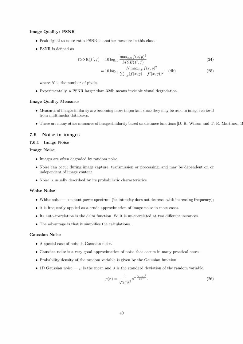
Image Quality: PSNR

• Peak signal to noise ratio PSNR is another measure in this class.

• PSNR is defined as

PSNR(f ′, f) = 10 log10

maxx,y f(x, y)2

MSE(f ′, f)(24)

= 10 log10

N maxx,y f(x, y)2∑x,y(f(x, y)− f ′(x, y))2

(db) (25)

where N is the number of pixels.

• Experimentally, a PSNR larger than 32db means invisible visual degradation.

Image Quality Measures

• Measures of image similarity are becoming more important since they may be used in image retrievalfrom multimedia databases.

• There are many other measures of image similarity based on distance functions [D. R. Wilson and T. R. Martinez, 1997].

7.6 Noise in images

7.6.1 Image Noise

Image Noise

• Images are often degraded by random noise.

• Noise can occur during image capture, transmission or processing, and may be dependent on orindependent of image content.

• Noise is usually described by its probabilistic characteristics.

White Noise

• White noise — constant power spectrum (its intensity does not decrease with increasing frequency);

• it is frequently applied as a crude approximation of image noise in most cases.

• Its auto-correlation is the delta function. So it is un-correlated at two different instances.

• The advantage is that it simplifies the calculations.

Gaussian Noise

• A special case of noise is Gaussian noise.

• Gaussian noise is a very good approximation of noise that occurs in many practical cases.

• Probability density of the random variable is given by the Gaussian function.

• 1D Gaussian noise — µ is the mean and σ is the standard deviation of the random variable.

p(x) =1√

2πσ2e−

(x−µ)2

2σ2 . (26)

40

7.6.2 Noise Type

Noise Type: additive

• Noise may be

additive the noise ν and image signal g are independent

f(x, y) = g(x, y) + ν(x, y). (27)

• During image transmission, noise is usually independent of the image signal occurs.

• The degradation can be modeled as additive noise.

Noise Type: multiplicative and impulse

• Noise may be

multiplicative the noise is a function of signal magnitude

f(x, y) = g(x, y) + ν(x, y)g(x, y) (28)= g(x, y)(1 + ν(x, y)) (29)= g(x, y)n(x, y). (30)

impulse an image is corrupted with individual noisy pixels whose brightness differs significantlyfrom that of the neighborhood.

Noise: discussions

• The term “salt and pepper noise” is used to describe saturated impulsive noise — an image cor-rupted with white and/or black pixel is an example.

• The problem of suppressing noise in images is addressed in subsequent lectures of this course.

7.6.3 Simulation of noise

Simulation of Gaussian Noise

• We first consider the simulation of Gaussian noise.

•

Theorem 7.1. (Box-Muller Method) Let U1 and U2 be i.i.d (independent identical distributed)uniformly distributed random variables on (0, 1). Then the random variables

N1 =√−2 logU1 cos(2πU2) (31)

N2 =√−2 logU1 sin(2πU2) (32)

are independent standard Gaussian.

Proof of Box-Muller Method I

• To prove it we need the following

•

Theorem 7.2. (Transformation Theorem for Densities) Let Z1, Z2 and U1, U2 be random variables.Assume

– (U1, U2) takes values in the open set G′ of R2 and has density f on G′;

41

– (Z1, Z2) takes values in the open set G of R2;

– ϕ : G 7−→ G′ is a continuously differentiable bijection with continuously differentiable inverseϕ−1 : G′ = ϕ(G) 7−→ G.

Given (U1

U2

)= ϕ

(Z1

Z2

). (33)

the random vector (Z1, Z2) on G has the density

g(z) = f ◦ ϕ(z)|Jϕ(z)| (34)

where Jϕ(z) = ∂(ϕ1,ϕ2)∂(z1,z2) is the Jacobian of ϕ.

Proof of Box-Muller Method II

• Frst we determine the map ϕ from the last theorem.

• We have

N21 = −2 logU1 cos2(2πU2) (35)

N22 = −2 logU1 sin2(2πU2). (36)

• HenceN2

1 +N22 = −2 logU1 (37)

andU1 = e−

N21 +N2

22 . (38)

• Moreover, by (31),N2

N1= tan(2πU2), (39)

i.e.,

U2 =1

2πarctan

(N2

N1

). (40)

Proof of Box-Muller Method III

• Hence

ϕ(z1, z2) =

(e−

z21+z222

12π arctan( z2z1 )

)(41)

• The transform domains are

G = R2 \ [{z1 = 0} ∪ {z2 = 0 and z1 > 0}], (42)

G′ = (0, 1)× (0, 1) \ {u2 =14

or u2 =34}. (43)

42

Proof of Box-Muller Method IV

• The partial derivatives of ϕ are

∂ϕ1

∂z1(z) = −z1e−

z21+z222 ,

∂ϕ1

∂z2(z) = −z2e−

z21+z222 (44)

∂ϕ1

∂z1(z) =

12π

−z2

z21 + z2

2

,∂ϕ1

∂z2(z) =

12π

z1

z21 + z2

2

. (45)

• It follows thatJϕ(z) =

12π

e−z21+z22

2 =1√2π

e−z212 · 1√

2πe−

z222 . (46)

Proof of Box-Muller Method V

• Since (U1, U2) has density χ(0,1)×(0,1), which is identically 1 on χ(0,1)×(0,1), (N1, N2) has density

1√2π

e−z212 · 1√

2πe−

z222 (47)

on G. Therefore they are independent Gaussian variables. �

7.6.4 The rejection method

The Rejection Method I

• This method uses an auxiliary density for generation of random quantities from distributions notamenable to analytic treatment [Press et al., 1992].

• Consider the generation of samples from a density π.

• Consider also an auxiliary density q for which we know how to generate samples.

• The idea is to use q to make samples from π.

• The method is general enough to generate samples from π without knowing the complete expressionfor π.

The Rejection Method II

• It is extremely common in statistics to encounter such situations where the kernel of π is knownbut the constant ensuring it integrals to 1 cannot be obtained analytically.

• The only mathematical restriction over q is that there must exist a constant A such that

π(x) ≤ Aq(x) (48)

for every possible value of x.

The Rejection Method III

• The method consists of independently drawing X from q and U ∼ U [0, 1] and accepting X as asample generated from π if

AUq(X) ≤ π(X). (49)

Otherwise X is not accepted as a sample from π and the process must be reinitialized until a valueX is accepted.

• Hence the name of the method, which is also known as the acceptance/rejection method.

43

Proof of the Rejection Method I

• To prove the rejection procedure effectively generates samples from π, we need to show that thedensity function of X is a constant multiple of π, when conditioned by the acceptance condition(49).

• The joint density of (X,U) is f(x, u) = q(x)χ[0,1](u), by the independence between X and U andthe uniformity of U .

• The conditional probability is computed by the following formula:

Pr(A|B) =Pr(A,B)Pr(B)

. (50)

Proof of the Rejection Method II

Pr(X ≤ t|AUq(X) ≤ π(X)) = Pr(X ≤ t|U ≤ π(X)Aq(X)

)

=Pr(X ≤ t, U ≤ π(X)

Aq(X) )

Pr(U ≤ π(X)Aq(X) )

=

∫∞−∞

∫∞−∞ q(x)χ[0,1](u)χ{x≤t,u≤ π(x)

Aq(x)}(x, u) dxdu∫∞−∞

∫∞−∞ q(x)χ[0,1](u)χ{u≤ π(x)

Aq(x)}(x, u) dxdu

=

∫ t−∞ dx

∫ π(x)Aq(x)

0 q(x)χ[0,1](u) du∫∞−∞ dx

∫ π(x)Aq(x)

0 q(x)χ[0,1](u) du

=

∫ t−∞

π(x)Aq(x)q(x) dx∫∞

−∞π(x)Aq(x)q(x) dx

=

∫ t−∞ π(x) dx∫∞−∞ π(x) dx

.

Extension of the Rejection Method

• The samples to be generated can have any form: scalar, vector or matrix.

• In each case, the rejection step is based on a comparison of densities with aid of a scalar uniformrandom variable.

Discussions on the Rejection Method

• q should be a density that is easy to draw samples from.

• The overall acceptance probability is

Pr(U ≤ π(X)Aq(X)

) =1A

∫ ∞−∞

π(x) dx (51)

• Hence, A must be chosen as close as possible to∫∞−∞ π(x) dx.

44

Rejection Method for Truncated Distributions

• A special case of rejection sampling is given for truncated distributions.

• Let q be any density and π be its truncation to the region C, i.e., π = qχC ≤ q.

• Taking A = 1, the acceptance condition is

Uq(X) ≤ π(X) = qχC (52)

which is satisfied, almost surely, if and only if X ∈ C.

• Hence, to generate sample from q restricted to C, one simply has to draw sample from q and acceptit if and only if it is in C.

7.6.5 The Polar method

Polar Method

• This a variant of the Box-Muller method to generate standard normal deviates. It is due to G.Marsaglia.

• It is substantially faster than the Box-Muller method since it avoids the calculation of the trigono-metric functions (but still slower than other methods, [Knuth, 1981]) and it has essential perfectaccuracy.

Box-Muller Method Revisited

• The Box-Muller method may be rephrased as follows:

– given (W,Θ) uniformly distributed on [0, 1]× [0, 2π];

– the variables

N1 =√−2 logW cos(Θ) (53)

N2 =√−2 logW sin(Θ) (54)

are independent standard Gaussian.

• The rejection method allows us to sample directly from√W cos Θ and

√W sin Θ, thus avoiding to

calculate the sines and cosines.

Sampling√W cos Θ and

√W sin Θ

• Given (Z1, Z2) uniformly distributed on the unit disk;

• Z1 = R cos Θ and Z2 = R sin Θ in polar coordinates R,Θ;

• Then W = R2 and Θ have joint density

1πχ{|r|≤1}(

√W cos Θ,

√W sin Θ)|∂Z1, Z2

∂W,Θ| (55)

=1πχ(0,1]×[0,2π)

∣∣∣∣∣(

cos Θ2√W

sin Θ2√W

−√W sin Θ

√W cos Θ

)∣∣∣∣∣ (56)

=1

2πχ[0,1]×[0,2π) (57)

on (0, 1]× [0, 2π);

• Hence (W,Θ) constructed above is uniform and independent on (0, 1]× [0, 2π);

45

Box-Muller Method in Polar Representation

• Clearly W = Z21 + Z2

2 and cos Θ = Z1√W

, and sin Θ = Z2√W

;

• Then the Box-Muller transform can be written as

N1 =

√−2 logW

WZ1 (58)

N2 =

√−2 logW

WZ2 (59)

W = Z21 + Z2

2 (60)

Polar MethodTo sample from the unit disk, we adopt the truncated rejection method:

• sample (V1, V2) uniformly from [−1, 1]× [−1, 1];

• until 0 < V 21 + V 2

2 ≤ 1, set (Z1, Z2) = (V1, V2).

7.6.6 Poissonian noise

Poissonian noise

• Each image data Ii,j is the random sampling from a random variable, which is Poissonian distributedwith mean di,j .

• Usually those random variables are independent.

• Then we have

Pr(I|d) =∏i,j

Pr(Ii,j |di,j) =∏i,j

di,jIi,j

Ii,j !exp (−di,j) (61)

7.6.7 Mixed noise: Poissonian + Gaussian

Mixed noise: Poissonian + Gaussian

• In this model, the image data Ii,j consist of two parts,

Ii,j = Pi,j +Gi,j (62)

where

– Oi,j are the data from the object, which are independently Poissonian distributed randomvariables with mean di,j ;

– gi,j are real-valued random variables accounting for the noise that is present in the device andenvironment.

Homework: Image Quality and Image Noise

• Use images corrupted with various noises to demonstrated the performance of image quality mea-sures such as MSE (22), SNR (23) and PSNR (24), etc.

• Which measure do you think statitically reasonable?

• You cal also consider to use those measures from [D. R. Wilson and T. R. Martinez, 1997].

• Please refer to [Wang et al., 2004] and references therein.

46

8 Color Images

Color

• Human color perception adds a subjective layer on top of underlying objective physical properties— the wavelength of electromagnetic radiation.

• Consequently, color may be considered a psychophysical phenomenon.

• Color has long been used in painting, photography and films to display the surrounding world tohumans in a similar way in which it is perceived.

• There is considerable literature on the variants in the naming of colors across languages — a verysubtle affair.

Color Constancy

• The human visual system is not very precise in perceiving- color in absolute terms;

– if we wish to express our notion of color precisely,

– we would describe it relative to some widely used color which is used as a standard.

• There are whole industries which present images to humans, and hence a desire for color constancy.

• In computer vision, we have the advantage of using a camera as a measuring device, which yieldsmeasurements in absolute quantities.

Newton

• Newton reported in the 17th century that white light from the sun is a spectral mixture,

• and used the optical prism to perform decomposition.

• This was a radical idea to propose at time.

• Over 100 years later influential scientists and philosophers such as Goethe refused to believe it.

8.1 Physics of Color

Electromagnetic Spectrum

47

Visual Spectrum

• The electromagnetic spectrum visible to a human, is with the wavelength λ from approximately380 nm to 740 nm.

• The intensity of irradiation for different wavelengths λ is called the power spectrum (or powerspectrum distribution S(λ).

• Visible colors with the wavelengths shown are called spectral colors

Primary Colors

• Colors can be represented as combinations of the primary colors, e.g., red, green, and blue;

• For the purposes of standardization they have been defined as 700 nm, 546.1 nm, and 435.8 nm,respectively [Pratt, 1978].

• But this standardization does not imply that all colors can be synthesized as combinations of thesethree.

Surface Reflection

• Two predominant physical mechanisms describing what happens when a surface is irradiated.

• First, the surface reflection rebounds incoming energy in a similar way to a mirror.

• The spectrum of the reflected light remains the same as that of the illuminant and it is independentof the surface — recall that shiny metals ’do not have a color’.

Body Reflection

• Second, the energy diffuses into the material and reflects randomly from the internal pigment inthe matter.

• This mechanism is called body reflection and is predominant in dielectrics as plastic or paints.

• Colors are caused by the properties of pigment particles which absorb certain wavelengths fromthe incoming illuminant wavelength spectrum.

Surface and Body Reflections

48

Spectrophotometer

• Most sensors used for color capture, e.g., in cameras, do not have direct access to color;

• the exception is a spectrophotometer which in principle resembles Newton’s prism.

• Incoming irradiation is decomposed into spectral colors and intensity along the spectrum is mea-sured in a narrow wavelength band,

– for instance, by a mechanically moved point sensor.

• Actual spectrophotometers use diffraction gratings instead of a glass prism.

Multispectral images

• Light intensities measured in several narrow bands of wavelengths are collected in a vector describ-ing each pixel.

• Each spectral band is digitized independently and is represented by an individual digital imagefunction as if it were a monochromatic image.

• Multispectral images are commonly used in remote sensing from satellites, airborne sensors andin industry.

• Wavelength usually span from ultraviolet through the visible section to infrared.

• Seven or a dozen wavelength bands are common.

• For instance, the LANDSAT 4 satellite transmits digitized images in five spectral bands fromnear-ultraviolet to infrared.

8.2 Color Perceived by Humans

Receptors

• Evolution has developed a mechanism of indirect color sensing in humans and some animals.

• Three types of sensors receptive to the wavelength of incoming irradiation have been establishedin humans, thus the term trichromacy.

• Color sensitive receptors on the human retina are the cones.

• The other light sensitive receptors on the retina are the rods which are dedicated to sensingmonochromatically in low ambient light conditions.

Cones

• Cones are categorized into three types based on the sensed wavelength range

– S (short) with maximum sensitivity at ≈ 430 nm,

– M (medium) at ≈ 560 nm,

– L (long) at ≈ 610 nm.

• Cones S, M, L are occasionally called cones B, G and R, respectively.

• This is slightly misleading. We do not see red solely because an L cone is activated.

• Light with equally distributed wavelength spectrum looks white to a human, and an unbalancedspectrum appears as some shade of color.

49

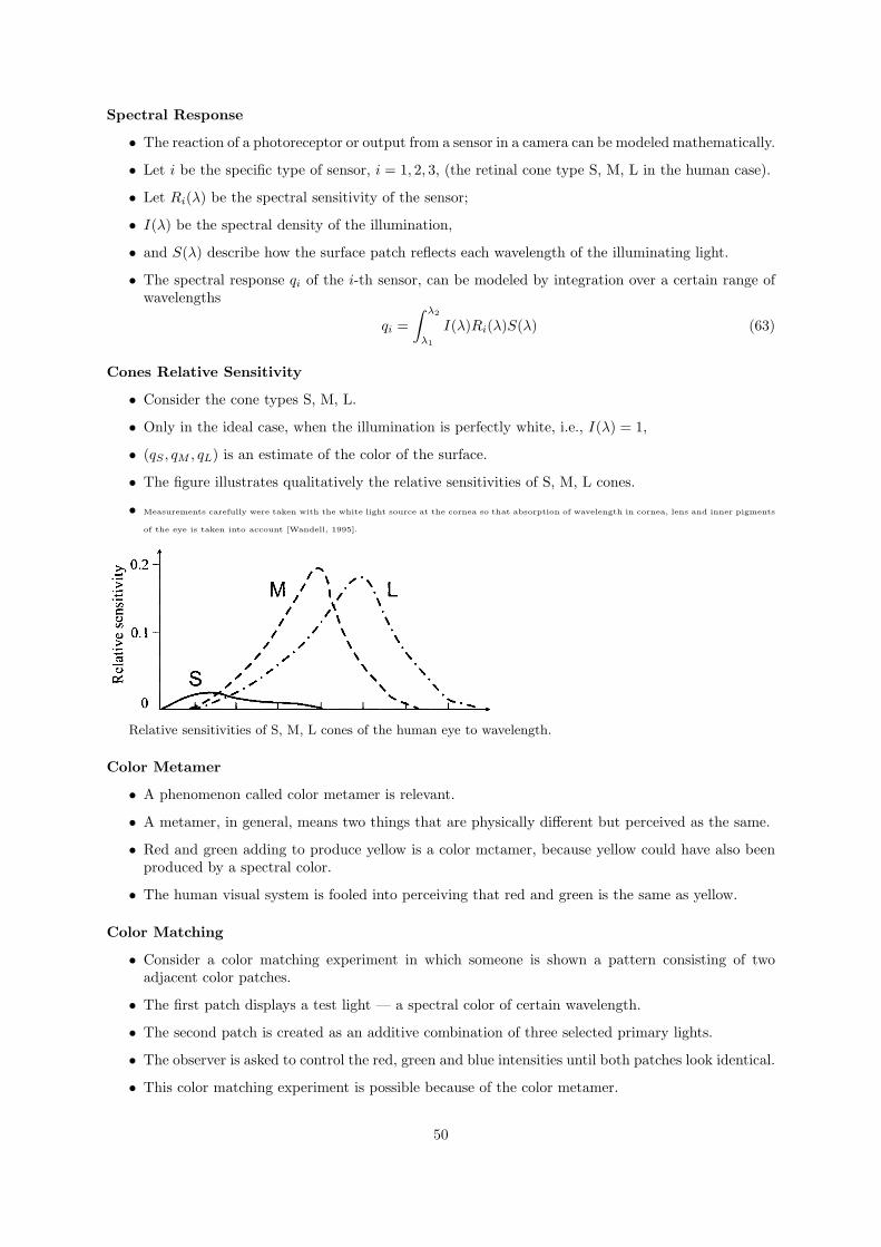
Spectral Response

• The reaction of a photoreceptor or output from a sensor in a camera can be modeled mathematically.

• Let i be the specific type of sensor, i = 1, 2, 3, (the retinal cone type S, M, L in the human case).

• Let Ri(λ) be the spectral sensitivity of the sensor;

• I(λ) be the spectral density of the illumination,

• and S(λ) describe how the surface patch reflects each wavelength of the illuminating light.

• The spectral response qi of the i-th sensor, can be modeled by integration over a certain range ofwavelengths

qi =∫ λ2

λ1

I(λ)Ri(λ)S(λ) (63)

Cones Relative Sensitivity

• Consider the cone types S, M, L.

• Only in the ideal case, when the illumination is perfectly white, i.e., I(λ) = 1,

• (qS , qM , qL) is an estimate of the color of the surface.

• The figure illustrates qualitatively the relative sensitivities of S, M, L cones.

• Measurements carefully were taken with the white light source at the cornea so that absorption of wavelength in cornea, lens and inner pigments

of the eye is taken into account [Wandell, 1995].

Relative sensitivities of S, M, L cones of the human eye to wavelength.

Color Metamer

• A phenomenon called color metamer is relevant.

• A metamer, in general, means two things that are physically different but perceived as the same.

• Red and green adding to produce yellow is a color mctamer, because yellow could have also beenproduced by a spectral color.

• The human visual system is fooled into perceiving that red and green is the same as yellow.

Color Matching

• Consider a color matching experiment in which someone is shown a pattern consisting of twoadjacent color patches.

• The first patch displays a test light — a spectral color of certain wavelength.

• The second patch is created as an additive combination of three selected primary lights.

• The observer is asked to control the red, green and blue intensities until both patches look identical.

• This color matching experiment is possible because of the color metamer.

50

Color Matching with Negative Values

• Negative lobes can be seen on the curves for red and green in this figure [Wandell, 1995].

• If the perceptual match has to be obtained then the observer has to add the intensity to the patchcorresponding to the spectral color.

• This increase of this intensity is depicted as a decrease in the color matching function. Hence thenegative values.

Color matching functions obtained in the color matching experiment. Intensities of the selected primary colors which perceptually match spectral

color of given wavelength λ.

Human Vision

• Human vision is prone to various illusions.

• Perceived color is influenced, besides the spectrum of the illuminant, by the colors and sceneinterpretation surrounding the observed color.

• In addition, eye adaptation to changing light conditions is not very fast and perception is influencedby adaptation.

• Nevertheless, we assume for simplicity that the spectrum of light coming to a point on the retinafully determines the color.

XYZ Color Space

• Color can be defined by almost any set of primaries;

• The world community agreed on primaries and color matching functions which are widely used.

• The color model was introduced as a mathematical abstraction allowing us to express colors astuples of numbers, typically as three or four values of color components.

• Being motivated by the press and the development of color film, CIE1 issued a technical standardcalled XYZ color space in 1931.

CIE Standard

• The standard is given by

– the three imaginary lights X = 700.0 nm, Y = 546.1 nm, Z = 435.8 nm,– the color matching functions X(λ), Y (λ) and Z(λ) corresponding to the perceptual ability of

an average human viewing a screen through an aperture providing a 2 deg field of view.

• The standard is artificial because there is no set of physically realizable primary lights that wouldyield the color matching functions in the color matching experiment.

• Nevertheless, if we wanted to characterize the imaginary lights then, very roughly speaking, X ≈red, Y ≈ green and Z ≈ blue.

1International Commission on Illumination, still acting in Lausanne, Switzerland.

51

XYZ Standards

• The XYZ color standard fulfills three requirements:

A Unlike the color matching experiment yielding negative lobes of color matching functions, thecolor matching functions of XYZ color space are required to be non-negative;

B The value of Y (λ) should coincide with the brightness (luminance);

C Normalization is performed to assure that the power corresponding to the three color matchingfunctions is equal (i.e., the area under all three curves is equal).

Color Match in XYZ

• A color is a mixture (more precisely a convex combination)

cXX + cY Y + cZZ (64)

where 0 ≤ cX , cY , cZ le1, are weights (intensities) in the mixture.

• The resulting color matching functions are shown in the figure [Wandell, 1995].

Color Gamut in XYZ

• The subspace of colors perceivable by humans is called the color gamut and is demonstrated inthe figure.

Projection View of Color Gamut in XYZ

• The projection plane is given by the plane passing through extremal points on all three axes, CIEchromaticity diagram.

52

• The new 2D coordinates (x, y) are obtained as

x =X

X + Y + Z, (65)

y =Y

X + Y + Z, (66)

z = 1− x− y. (67)

All monochromatic spectra visible to humans map into the curved part of the horseshoe. The triangledepicts a subset of colors spanned by red, green, and blue.

Color Gamuts in XYZ

• Display and printing devices use three selected real primary colors (as opposed to three syntacticprimary colors of XYZ color space).

• All possible mixtures of these primary colors fail to cover the whole interior of the horseshoe inCIE chromaticity diagram.

• This situation is demonstrated qualitatively for three particular devices.

Other Standards

• The CIE standard is an example of an absolute standard, i.e., defining unambiguous representationof color which does not depend on other external factors.

• There are more recent and more precise absolute standards: CIELAB 1976 (ISO 13665) and Hunter-Lab (www.hunterlab.com).

• Later, we will also discuss relative color standards such as RGB color space.

• There are several RGB color spaces used — two computer devices may display the same RGBimage differently.

53

8.3 Color Spaces

Color Spaces

• Several different primary colors and corresponding color spaces are used in practice, and thesespaces can be transformed into each other.

• If the absolute color space is used then the transformation is the one-to-one mapping and does notlose information (except for rounding errors).

• Because color spaces have their own gamuts, information is lost if the transformed value appearsout of the gamut.

RGB Color Space

• The RGB color space has its origin in color television where Cathode Ray Tubes (CRT) were used.

• RGB color space is an example of a relative color standard (as opposed to the absolute one, e.g.,CIE 1931).

• The primary colors (R-red, G-green and B-blue) mimicked phosphor in CRT luminophore.

• The RGB model uses additive color mixing to inform what kind of light needs to be emitted toproduce a given color.

• The value of a particular color is expressed as a vector of three elements — intensities of threeprimary colors.

• A transformation to a different color space is expressed by a transformation by a 3× 3 matrix.

RGB Representation

• Assume that values for each primary are quantized to m = 2n values;

• let the highest intensity value be k = m− 1;

• then (0, 0, 0) is black, (k, k, k) is (television) white, (k, 0, 0) is ’pure’ red, and so on.

• The value k = 255 = 28 − 1 is common, i.e., 8 bits per color channel.

• There are 2563 = 224 = 16, 777, 216 possible colors in such a discretized space.

RGB Color Space Diagram

• RGB color space with primary colors red, green, blue and secondary colors yellow, cyan, magenta.

• Gray-scale images with all intensities lie along the dashed line connecting black and white colorsin RGB color space.

• The RGB model may be thought of as a 3D co-ordinatization of color space; note the secondarycolors which are combinations of two pure primaries.

54

RGB vs XYZ

• There are specific instances of the RGB color model as sRGB, Adobe RGB and Adobe Wide GamutRGB.

• They differ slightly in transformation matrices and the gamut.

• One of transformations between RGB and XYZ color spaces is

YIQ Color Space

• The US and Japanese color television formerly used YIQ color space.

• The Y component describes intensity

• and I, Q represent colors, corresponding approximately to the amounts of blue and red in the color.

• YIQ is another example of additive color mixing.

YUV Color Space

• This color space corresponds closely to the YUV color model in the PAL television norm.

• YIQ color space is rotated 33 deg with respect to the YUV color space.

• The YIQ color model is useful since the Y component provides all that is necessary for a monochromedisplay;

• It exploits advantageous properties of the human visual system, in particular our sensitivity toluminance.

CMY Color Space

• The CMY — for Cyan, Magenta, Yellow — color model uses subtractive color mixing which isused in printing processes.

• It describes what kind of inks need to be applied so the light reflected from the white substrate(paper, painter’s canvas) and passing through the inks produces a given color.

• CMYK stores ink values for black in addition.

• Black color can be generated from C, M, Y components.

• As it is abundant in printed documents, it is of advantage to have a special black ink.

• Many CMYK colors spaces are used for different sets of inks, substrates, and press characteristics(which change the color transfer function for each ink and thus change the appearance).

55

HSV Color Space

• HSV — Hue, Saturation, and Value (also known as HSB, hue, saturation, brightness) is often usedby painters because it is closer to their thinking and technique.

• Artists commonly use three to four dozen colors (characterized by the hue; technically, the dominantwavelength).

• If another color is to be obtained then it is mixed from the given ones.

• The painter also wants colors of different saturation.

• E.g., to change ’fire brigade red’ to pink, she will mix the ’fire brigade red’ with white (andor black)to obtain the desired lower saturation.

HSV Color Model

HSV, HSL, HSI

• HSV decouples intensity information from color, while hue and saturation correspond to humanperception.

• This representation is very useful for developing image processing algorithms.

• This will become clearer as we proceed to describe image enhancement algorithms.

• HSL (hue, saturation, lightness/luminance), also known as HLS or HSI (hue, saturation, intensity)is similar to HSV.

• ’Lightness’ replaces ’brightness’.

• The difference is that the brightness of a pure color is equal to the brightness of white,while the lightness of a pure color is equal to the lightness of a medium gray.

Summary

• Be careful for formulas in books.

56

Multi-spectral image demonstration

• Multi-spectral image captured by Land-sat TM-5.

• The example uses the images from its 3rd, 4th and 5th spectral bands.

• The matlab script for this example is multi spectral image.m.

8.4 Palette Images

Palette Images

• Palette images (indexed images) provide a simple way to reduce the amount of data needed torepresent an image.

• The pixel values constitute a link to a lookup table of colors (also called a color table, colormap, index register, palette).

• The lookup table contains as many entries as the range of possible values in the pixel, typically8 bits = 256 values.

• Each entry of the table maps the pixel value to the color, so there are three values, one for each ofthree color components.

• This approach would reduce data size to 1/3 (plus size of the look up table).

Image Formats

• In the RGB color model, values for red, green and blue are provided.

• Image formats for raster images such as TIFF, PNG and GIF can store palette images.

(image from www.mathworks.com)

Not Enough Colors?

• If the number of colors in the input image is less than or equal to the number of entries in thelookup table,

• then all colors can be selected and no loss of information occurs.

• Such images may be cartoon movies, or program outputs.

• In the more common case,

– the number of colors in the image exceeds the number of entries in the lookup table

– a subset of colors has to be chosen,

• and a loss of information occurs.

57

http://www.mathworks.com/access/helpdesk/help/techdoc/creating_plots/chimage9.gif

Color Selection

• This color selection may be done many ways.

• The simplest is to quantize color space regularly into cubes of the same size.

• In the 8 bit example,

– there would be 8× 8× 8 = 256 cubes.– for a green frog in green grass there will not be enough shades of green in the lookup table to

display the image well.

• It is better to

– check which colors appear in the image by creating histograms for all three color components– quantize them to provide more shades for colors which occur in the image frequently.

• If an image is converted to a palette representation then the nearest color in the lookup table isused to represent the color.

Pseudocolor

• The term pseudocolor is usually used when an original image is gray-level and is displayed incolor;

– this is often done to exploit the color discriminatory power of human vision.

• The same palette machinery as described above is used for this purpose;

– a palette is loaded into the lookup table which visualizes the particular gray-scale image thebest.

• It could either enhance local changes, or might provide various views of the image.

• Which palette to choose is an issue.

8.5 Color Constancy

Color Constancy: a challenging problem

• Consider the situation in which the same surface is seen under different illumination.

• The same surface colors are shown fully illuminated and in shadow.

• The human vision system is able to abstract to a certain degree from the illumination changes andperceive several instances of a particular color as the same.

• This phenomenon is called color constancy.

Part III

Data structures for image analysisOutline

58

Contents

Data and Algorithm

• Data and an algorithm are the two basic parts of any program.

• Computer program = data + algorithm.

• Data organization can considerably affect the simplicity of the selection and the implementationof an algorithm.

• The choice of data structures is fundamental when writing a program.

Inappropriate Representation for Images

• The difficulties in image processing, image analysis and computer vision come from the bad repre-sentation or organization of the data involved.

• In fact, the visual information representation and organization inside human brain is not wellunderstood at present.

• Although we are to discuss some representations used so far, none of them are appropriate for ageneral purpose processing target.

9 Levels of Representation

Levels of Representation

• The aim of computer visual perception is to find a relation between an input image and the modelsof the real world.

• During the transition from the raw image to the model, semantic knowledge about the interpre-tation of image data is used more and more.

• Several levels of visual information representation are defined on the way between the input imagethe model.

Levels of Representation and Algorithms

• Computer vision then comprises a design of the

– Intermediate representations (data structures).

– Algorithms used for the creation of representation and introduction of relations between them.

Four Levels of Representations

• The representation can be stratified in four levels.

– Iconic images

– Segmented images

– Geometric representations

– Relational models

59

Discussions on Four Levels of Representations

• However, there are no strict borders between them and a more detailed classification of the repre-sentational levels may be used in some applications.

• For some specific uses, some representations can be omitted.

• These four representational levels are ordered from signals at low level of abstraction to the de-scription that a human can understand.

• The information flow between the levels may be bi-directional.

Iconic Images

• Iconic images — consists of images containing original data; integer matrices with data aboutpixel brightness.

• E.g., outputs of pre-processing operations (e.g., filtration or edge sharpening) used for highlightingsome aspects of the image important for further treatment.

Segmented Images

• Segmented images — parts of the image are joined into groups that probably belong to the sameobjects.

• E.g., the output of the segmentation of a scene with polyhedrons is either line segments coincidingwith borders or two-dimensional regions corresponding with faces of bodies.

• It is useful to know something about the application domain while doing image segmentation; it isthen easier to deal with noise and other problems associated with erroneous image data.

Geometric Representations

• Geometric representations — hold knowledge about 2D and 3D shapes.

• The quantification of a shape is very difficult but very important.

• It is the inverse problem of computer graphics.

Relational Models

• Relational models - give the ability to treat data more efficiently and at a higher level of ab-straction.

• A priori knowledge about the case being solved is usually used in processing of this kind.

• Example - counting planes standing at an airport using satellite images

– position of the airport (e.g., from a map).

– relations to other objects in the image ( e.g., to roads, lakes, urban areas).

– geometric models of planes for which we are searching.

– etc.

• AI techniques are often explored.

• Information gained from the image may be represented by semantic nets or frames.

60

10 Traditional Image Data Structures

Traditional Image Data Structures

• Traditional image data structures, such as

– matrices

– chains

– graphs

– lists of object properties

– relational databases

– etc.

are important not only for the direct representation of image information, but also a basis of morecomplex hierarchical methods of image representation.

10.1 Matrices

Matrices

• This is the most common data structure for low level image representation.

• Elements of the matrix are integer, real or complex numbers, corresponding to brightness, or toanother property of the corresponding pixel of the sampling grid.

• Image data of this kind are usually the direct output of the image capturing device, e.g., a scanner.

• Pixels of both rectangular and hexagonal sampling grids (Fig. 96) can be represented by a matrix.

• The correspondence between data and matrix elements is obvious for a rectangular grid; with ahexagonal grid every row in the image is shifted half a pixel to the right or left.

Images Represented by Matrices

• Some special images that are represented by matrices are:

– Binary images (an image with two brightness levels only) is represented by a matrix containingzeros and ones.

– Several matrices can contain information about one multi-spectral image. Each of thesematrices contains one image corresponding to one spectral band.

– Matrices of different resolution are used to obtain hierarchical image data structures.

– A representation of a segmented image by a matrix usually saves memory than an explicitlist of all spatial relations between all objects, although sometimes we need to record otherrelations among objects.

Images = Matrices = Arrays

• Image information in the matrix is accessible through the co-ordinates of a pixel that correspondwith row and column indexes.

• Most programming language use a standard array data structure to represent a matrix.

61

Images = Matrices = Arrays in C

• In C, an image of 256 gray-levels with dimension M ×N can be stored in a two dimensional array

unsigned char image [M][N]

• The above stored array may be dis-continuous in memory.

• Then another way to represent the image is by a one-dimensional array, which is continuous in thememory

unsigned char image [M * N]

• We need to know the image dimension M and N usually.

Images = Matrices = Structure in C (I)

• Another method is to represent an image by a structure type,

typedef struct image{

int rows;int columns;char *values;¡other useful information¿;

} Image;

or use a pointer to the above structure

typedef Image * ImageX;

or declared astypedef struct image * ImageX;

Images = Matrices = Structure in C (II)

• When initialized,

value = (char *) malloc (sizeof(char) * rows * columns);

• To access one element of the matrix at pixel (m,n), use the following macro

#define Pixel(IX, m, n)(IX-¿values[m*(IX-¿columns)+n])

where 0 ≤ m ≤M − 1 and 0 ≤ n ≤ N − 1.

Other Image Data Types

• You may use other type such asfloat *values;

ordouble *values;

to implement much precise computation.

62

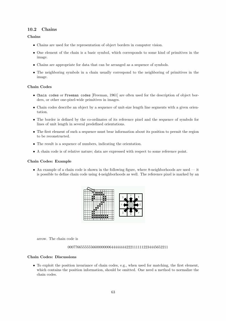
10.2 Chains

Chains

• Chains are used for the representation of object borders in computer vision.

• One element of the chain is a basic symbol, which corresponds to some kind of primitives in theimage.

• Chains are appropriate for data that can be arranged as a sequence of symbols.

• The neighboring symbols in a chain usually correspond to the neighboring of primitives in theimage.

Chain Codes

• Chain codes or Freeman codes [Freeman, 1961] are often used for the description of object bor-ders, or other one-pixel-wide primitives in images.

• Chain codes describe an object by a sequence of unit-size length line segments with a given orien-tation.

• The border is defined by the co-ordinates of its reference pixel and the sequence of symbols forlines of unit length in several predefined orientations.

• The first element of such a sequence must bear information about its position to permit the regionto be reconstructed.

• The result is a sequence of numbers, indicating the orientation.

• A chain code is of relative nature; data are expressed with respect to some reference point.

Chain Codes: Example

• An example of a chain code is shown in the following figure, where 8-neighborhoods are used — itis possible to define chain code using 4-neighborhoods as well. The reference pixel is marked by an

arrow. The chain code is

00077665555556600000006444444442221111112234445652211

Chain Codes: Discussions

• To exploit the position invariance of chain codes, e.g., when used for matching, the first element,which contains the position information, should be omitted. One need a method to normalize thechain codes.

63

• A chain code is very sensitive to noise and arbitrary changes in scale and rotation may causeproblems if used fro recognition.

• The description of an image by chains is appropriate for syntactic pattern recognition that is basedon formal language theory approaches.

• Chains can be represented using static data structures (e.g., 1D arrays); their size is the longestlength of the chain expected.

• Dynamic data structures are more advantageous to save memory.

10.3 Topological Data Structures

Topological Data Structures by Graphs

• Topological data structures describe the image as a set of elements and their relations.

• These relations are often represented using graphs.

• A graph G = (V,E) is an algebraic structure which consists of a set of nodes

V = {v1, v2, · · · , vn}, (68)

and a set of arcsE = {e1, e2, · · · , em}. (69)

• Each arc ek is naturally connected with an unordered pair of nodes {vi, vj} which are not necessarilydistinct.

• The degree of the node is equal to the number of incident arcs of the node.

Evaluated Graphs

• An evaluated graph is a graph in which values are assigned to arcs, to nodes or to both — thesevalues may, e.g., represent weights, or costs.

Region Adjacency Graphs

• The region adjacency graph is typical of this class of data structures.

• Nodes correspond to regions and neighboring regions are connected by an arc.

• The segmented image consists of regions of pixels with similar properties (brightness, texture, color,...) that correspond to some entities in the scene.

• The neighborhood relation is fulfilled when the regions have some common border.

Region Adjacency Graphs: ExampleAn example of an image with regions labeled by numbers and corresponding region adjacency graph

is shown in the following figure The label 0 is denotes pixels out of the image. This value is used toindicate regions that touch borders of the image in the region adjacency graph.

Region Adjacency Graphs: Discussions

• The region adjacency graph has several attractive features.

• If a region enclose other regions, then the part of the graph corresponding with the areas insidecan be separated by a cut in the graph.

• Nodes of degree 1 represent simple holes.

• The region adjacency graph can be used for matching with a stored pattern for recognition purpose.

64

Region Adjacency Graphs: Creation

• The region adjacency graph is usually created from the region map, which is a matrix of the samedimension as the original image matrix whose elements are identification labels of the regions.

• To created the region adjacency graph, borders of all regions in the image are traced, and labelsof all neighboring regions are stored.

• The region adjacency graph can easily be created from an image represented by a quadtree in§ 11.2 as well.

10.4 Relational Structures

Relational Structures

• Relational databases can also be used for representation of information from an image.

• All the information is then concentrated in relations between semantically important parts of theimage — objects — that are the result of segmentation.

• Relations are recorded in the form of tables.

• Individual objects are associated with their names and other features, e.g., the top-left pixel of thecorresponding region in the image.

• Relations between objects are expressed in the relational table as well.

Relational Structures: ExampleAn example of such a representation is shown in the following figure and table.

(a) Image (b) Database

Relational Structures: Discussions

• Description by means of relational structures is appropriate for higher level image understanding.

• Search using keys, similar to database searches, can be used to speed up the whole process.

65

11 Hierarchical Data Structures

Huge Dataset

• Computer vision is by its nature very computationally expensive, if for no other reason than thelarge amount of data to be processed.

• Systems which we might call sophisticated must process considerable quantities of image data —hundreds of kilobytes to tens of megabytes.

• The visual information perceived by the two human eyes is about 3000 MB/s (add reference orestimate it!!!).

• One of the solutions is using parallel computers (in other words brute force).

• Unfortunately many computer vision problems are difficult to divide among processors, or decom-pose in any way.

Hierarchical Data Structures

• Hierarchical data structures make it possible to use algorithms which decide a strategy forprocessing on the basis of relatively small quantities of data.

• They work at the finest resolution only with those parts of the image for which it is necessary,using knowledge instead of brute force to ease and speed up the processing.

• We are going to introduce two typical hierarchical structures, pyramids and quadtrees.

11.1 Pyramids

Pyramids

• Pyramids are among the simplest hierarchical data structures.

• We distinguish between M-pyramids (matrix pyramids) and T-pyramids (tree pyramids).

M-Pyramids

• A M-pyramid is a sequence {ML,ML−1, · · · ,M0} of images.

• ML has the same dimensions and elements as the original image.

• Mi−1 is derived from the Mi by reducing the resolution, usually, by one half.

M-Pyramids: Creation

• When creating pyramids, it is customary to work with square matrices with dimensions equal topowers of 2.

• For images with arbitrary dimensions, a resampling procedure is needed in creating the pyramids.

• M0 corresponds to one pixel only.

• The number of image pixels used by an M-pyramid for storing all matrices is

N2

(1 +

14

+116

+ · · ·)

= 1.33N2

M-Pyramids: Discussions

• M-pyramid created by shrinking the image dimensions. The matlab script for this example ism pyramid.m.

66

M-Pyramids: Discussions

• M-pyramids are used when it is necessary to work with an image at different resolutions simulta-neously.

• An image having one degree smaller resolution in a pyramid contains four times less data, so thatit is processed approximately four times as quickly.

T-Pyramids

• Often it is advantageous to use several images of the same resolution simultaneously rather thanto create just one image at a resolution in the M-pyramid.

• E.g., we use images at a resolution, containing additional information at this resolution, texture,orientation and segmentation properties, etc.

• Such images can be represented using tree pyramids — T-pyramids.

• The following figure is a example T-pyramid tree. Every node of the T-pyramid has 4 child nodes.

11.2 Quadtrees

Quadtrees

• Quadtrees are modifications of T-pyramids.

• Every node of the tree except the leaves has four children (NW: north-western, NE: north-eastern,SW: south-western, SE: south-eastern).

• The image is divided into four quadrants at each hierarchical level, though it is not necessary tokeep nodes at all levels.

• If a parent node has four children of the same (e.g., brightness) value, (which is often characterizedby a similarity measure), it is not necessary to record them.

67

Quadtrees: Structures

• Quadtrees are usually represented by recording the whole tree as a list of its individual nodes.

• Every node being a record with several items characterizing it.

• An example is given as following

node = {node type,pointer to NW son,pointer to NE son,pointer to SW son,pointer to SE son,pointer to Father,other data

}

• In the item “node type”, there is information about whether the node is a leaf or inside the tree.

• “other data” can be the level of the node in the tree, position in the picture, brightness for thisnode, etc.

• This kind of representation is redundant and expansive in memory. Its advantage is easy access toany node.

Quadtrees: Example

• Launch matlab, run the demo “qtdemo”.

• matlab uses sparse matrix to store the quadtree decomposition, without the brightness value in-formation for each node or block.

Quadtrees: Discussions

• Disadvantages associated with image pyramid representation:

– Dependence on the position, orientation and relative size of objects.

– Two similar images with just very small differences can have very different pyramid or quadtreerepresentations.

– Even two images depicting the same, slightly shifted scene, can have entirely different repre-sentations.

– These disadvantages can be overcome using a normalized shape of quadtree in which do notcreate the quadtree for the whole image, but for its individual objects.

– Please refer the text book for further discussions.

Part IV

Image Pre-processingPre-processing

• Pre-processing is a common name for operations with images at the lowest level of abstraction —both input and output are intensity images.

68

• These iconic images are of the same kind as the original data captured, with an intensity imageusually represented by a matrix of image function values (brightness).

• The aim of pre-processing is an improvement of the image data that suppresses unwanted distortionsor enhances some image features important for further processing.

Pre-processing: Classification

• Four categories of image pre-processing methods according to the size of the pixel neighborhoodthat is used for the calculation of a new pixel brightness:

– pixel brightness transformations.

– geometric transformations.

– pre-processing methods that use a local neighborhood of the processed pixel.

– image restoration that requires knowledge about the entire image.

• Other classifications of image pre-processing methods exist.

Pre-processing: basic idea

• Image pre-processing methods use the considerable redundancy in images.

• Neighboring pixels corresponding to one object in real images have essentially the same or similarbrightness value — spatial coherence or spatial correlation.

• Thus, distorted pixel can often be restored as an average value of neighboring pixels.

Pre-processing: a priori information

• If pre-processing aims to correct some degradation in the image, the nature of a priori informationis important and is used to different extent:

– no knowledge about the nature of the degradation is used; only very general properties of thedegradation are assumed.

– using knowledge about the properties of the image acquisition device, and conditions underwhich the image was obtained. The nature of noise (usually its spectral characteristics) issometimes known.

– using knowledge about objects that are searched for in the image, which may simplify thepre-processing quite considerably.

• If knowledge about objects is not available in advance it can be estimated during the processing.

Pre-processing: Strategy

• The following strategy is possible.

– First the image is coarsely processed to reduce data quantity and to find image objects.

– The image information derived is used to create a hypothesis about image object propertiesand this hypothesis is then verified in the image at finer resolution.

– Such an iterative process cab be repeated until the presence of knowledge is verified or rejected.

– This feedback may span more than pre-processing, since segmentation also yields semanticknowledge about objects — thus feedback can be initiated after the object segmentation.

69

12 Pixel Brightness Transformations

Pixel Brightness Transformations

• Brightness transformations modify pixel brightness — the transformation depends on the propertiesof a pixel itself.

• There are two brightness transformations:

• Brightness corrections

– consider the original brightness

– and pixel position in the image.

• Gray scale transformation

– change brightness without regard to position in the image.

12.1 Position dependent brightness correction

Position dependent brightness correction

• Ideally, the sensitivity of image acquisition and digitization devices should not depend on positionin the image, but this assumption is not valid in practice.

• Sources of degradation:

– non-homogeneous property of optical system;The lens attenuates light more if it passes farther from the optical axis.

– non-homogeneous sensitivity of light sensors;The photo sensitive part of the sensor (vacuum-tube camera, CCD camera elements) is notof identical sensitivity.

– non-homogeneous object illumination.

• Systematic degradation can be suppressed by brightness correction.

Multipilcation Degradation

• Let a multiplicative error coefficient e(i, j) describe the change from the ideal identity transferfunction

– g(i, j) is the original undegraded image (or desired image);

– f(i, j) is the image containing degradation.

f(i, j) = e(i, j)g(i, j) (70)

Correction for Multipilcation Degradation

• If a reference image gc(i, j) is known (e.g., constant brightness c)

– the degraded result is fc(i, j)

– systematic brightness errors can be suppressed:

g(i, j) =f(i, j)e(i, j)

=gc(i, j)f(i, j)

fc(i, j)=

c

fc(i, j)f(i, j) (71)

70

Discussions I

• This method can be used only if the image degradation process is stable.

• If we wish to suppress this kind of degradation in the image capture process, we should calibratethe device from time to time (find error coefficients e(i, j))

• This method implicitly assumes linearity of the transformation, which is not true in reality as thebrightness scale is limited into some interval.

– overflow is possible in (71). Then the limits of the brightness scale are used instead in (71).

– The best reference image should have brightness that is far enough from both limits.

Discussions II

• If the gray scale has 256 brightnesses the ideal image has constant brightness value 128.

– Most TV/DV cameras have automatic control of the gain which allows them to operate underchanging illumination conditions.

– If systematic errors are suppressed using error coefficients, this automatic gain control shouldbe switched off first.

Brightness Correction Example

• The matlab script for this example is brightness correction.m.

12.2 Grey scale transformation

Grey scale transformation

• Grey scale transformations do not depend on the position of the pixel in the image.

• Brightness transform is a monotonic function:

q = T (p) (72)

– a - Negative transformation

– b - contrast enhancement (between p1 and p2)

– c - Brightness thresholding

Some Other Examples

71

Look-up Tables

• Grey scale transformations can be performed using look-up tables.

• Grey scale transformations are mostly used if the result is viewed by a human.

12.2.1 Windows and level

Windows and level

• It is an interactive contrast enhancement tool.

• It is an expansion of the contrast of pixels within a given window range.

• Two parameters define the range: the middle point Level, and the width of the range Window.

• Another name for this operation is Intensity of Interest (IOI).

Figure 10: A graphic visualization of this process.

Example I

(a) Original (b) Hisogram (c) After Windows andLevel Contrast Change

Figure 11: First find the minimum and maximum values, decide the initial value, bin-width and numberof bins for computing the histogram. From the histogram, chose the lower and upper cutoff value.

Example II

74

(a) Original (b) Hisogram (c) After Windowsand Level ContrastChange

12.2.2 Histogram stretching

Histogram stretching

• Histogram stretching can be seen as a Window and Level contrast enhancement technique wherethe window ranges from the minimum to the maximum pixel values of the image.

• This normalization or histogram stretching operation is automatically performed in many displayoperators.

• To fully illustrate the difference between the two displayed images a gray level scale was superim-posed in both images to guarantee that the display operator will use the same gray-level scale.

12.2.3 Histogram Equalization

Histogram Equalization I

• Histogram equalization is to produce an image with equally distributed brightness levelsover the whole brightness scale.

Histogram Equalization II

• Let H(p) be the input histogram and the input gray-scale range be [p0, pk].

• We are to find a monotonic pixel brightness transform q = T (p) such that the output histogramG(q) is uniform over the whole output brightness scale [q0, qk].

• The histogram is a discrete probability density function.

• The monotonic property of the transform T implies

j∑i=0

G(qi) =j∑i=0

H(pi) (73)

where qi = T (pi).

• The sum in the above equation can be interpreted as discrete distribution function.

75

Histogram Equalization III

• Assume that the image has M rows and N columns. The total number of pixels is MN .

• The equalized histogram corresponding to the uniform probability density function f whose func-tion value satisfies

f(q)(qk − q0) = MN. (74)

• The continuous version of (73) is∫ q

q0

f(r) dr =∫ p

p0

H(s) ds, q = T (p). (75)

• Therefore, we obtain,

MN

∫ q

q0

1qk − q0

dr =MN(q − q0)qk − q0

=∫ p

p0

H(s) ds. (76)

Histogram Equalization IV

• The desired pixel brightness transformation T can then be derived as

q = T (p) =qk − q0

MN

∫ p

p0

H(s) ds+ q0. (77)

• The integral in the above equation is called the cumulative histogram, which is approximated by asum for digital images,

F [p] =∫ p

p0

H(s) ds =j∑i=0

H(pi), pj = round(p).

• Therefore, resulting histograms are not generally equalized ideally.

• The discrete approximation of the continuous pixel brightness transformation form the above equa-tion is

qj = T (pj) =qk − q0

MN

j∑i=0

H(pi) + q0. (78)

Histogram Equalization Algorithm

1. For an N×M image of G gray-levels (often 256), create two arrays H and T of length G initializedwith 0 values.

2. Form the image histogram: scan every pixel and increment the relevant member of H — if pixelX has intensity p, perform

H[p] = H[p] + 1 (79)

3. Form the cumulative image histogram Hc. We may use the same array H to stored the result.

H[0] = H[0]H[p] = H[p− 1] +H[p]

for p = 1, · · · , G− 1.

4. Set

T [p] = round[G− 1MN

H[p]]. (80)

Note the new gray-scale is assumed to be the same as the input image, i.e., qk = G− 1 and q0 = 0.

5. Rescan the image and write an output image with gray-levels q, setting

q = T [p]. (81)

76

(d) Images before and after histoeqlization (e) Hisograms

Example I

Example II

• The matlab script from visionbook is visionbook/05Preproc/hist equal demo.m.

DiscussionsThe following comments are from [Klette and Zamperoni, 1996, p. 148]:

• The gray value range equalization may be used for improving the image quality if the originalimage covers only a part of the full gray scale.

• An insufficient exploitation of the full gray scale is mostly due to image acquisition circumstances,as e.g., low scene illumination or automatic gain control of the camera.

• In case of good gray value dynamics of the input image, an equalization can lead even to qualitylosses in form of unsharp edges.

Example III

• Another histogram equalization example. The matlab script is ../program/histo eq demo.m.

• Some edges become unsharp.

12.2.4 Histogram Matching

Histogram Matching I

• Histogram matching is to produce an image with desired distributed brightness levels over thewhole brightness scale.

• Assume the desired probability density function is G(q).

• Let the desired pixel brightness transform be T .

• Similarly we have

F [p] =∫ q=T [p]

q0

G[s] ds (82)

where F [p] is the cumulative histogram of the input image. Assumed that the cumulative histogramis normalized in [0, 1].

• From the above equation, it is possible to find the transformation T .

77

Histogram Matching II

• E.g., if G is the exponential distribution,

G[q] = αe−α(q−q0) (83)

for q ≥ q0.

• We haveF [p] = 1− e−α(T [p]−q0) (84)

• Then we find the transformation

T [p] = q0 −1α

log(1− F [p]) (85)

• In the discrete case, the transformation can be implemented by building look-up tables.

HomeworkImplementation of those transforms are left as homework. The homework includes:

1. Grey scale transformations with given functions such as exponent, logarithm, user defined (by somecontrol points for a piece wise linear function), etc.;

2. Histogram stretching to a given range;

3. Histogram equalization;

4. Histogram matching: find other probability density functions in [Rongchun Zhao, 2000, p. 81].Implemente the histogram matching transforms for those probability density functions.

5. F Histogram matching to the histogram from a given image.

Note:

• Histograms should be plotted when histograms are involved.

• Your final score will also depend on the interface of your program.

• Be sure to give us a friendly interface.

• Be sure to choose illustrative images.

13 Geometric Transformations

Geometric Transformations

• Geometric transformations are common in computer graphics, and are often used in image analysis.

• Geometric transforms permit the elimination of geometric distortion that occurs when an image iscaptured.

• If one attempts to match two different images of the same object, a geometric transformation maybe needed:

– matching remotely sensed images of the same area taken after one year, when the recent imageis not taken from the same orientation and/or position.

– correcting for document skew in OCR, which occurs when an image with an obvious orientation(e.g., a printed page) is scanned, or otherwise captured, at a different orientation.

78


• A geometric transform is a vector function T that maps the pixel (x, y) to a new position (x′, y′),

x′ = Tx(x, y) y′ = Ty(x, y) (86)


• The transformation equations are

– either known in advance,– or can be determined from known original and transformed images,– or can be estimated from known obvious orientations (e.g., OCR applications).– Several pixels in both images with known correspondence are used to derive the unknown

transformation.


• A geometric transform consists of two basic steps:

1. determining the pixel co-ordinate transformation– mapping of the co-ordinates of the input image pixel to the point in the output image.– the output point co-ordinates should be computed as continuous values (real numbers) as

the position does not necessarily match the digital grid after the transform.2. determining the brightness of the points in the digital grid.


• The brightness values are usually computed as an interpolation of the brightnesses of several pointsin the neighborhood.

• This idea enables the classification of geometric transformation among other pre-processing tech-niques, the criterion being that only the neighborhood of a processed pixel is needed for thecalculation.

• Geometric transformations are on the boundary between point and local operations.

Geometric Transformations: Areas of Images

• A geometric transformation applied to the whole image may change the co-ordinate system, and aJacobean J provides information about how the co-ordinate system changes

J(x, y) =∂(x′, y′)∂(x, y)

(87)

• The area of the image is invariant if and only if |J | = 1.

79

13.1 Pixel Co-ordinate Transformations

13.1.1 Polynomial Approximation

Polynomial Approximation

• The transformation is usually approximated by a polynomial equation (of degree m)

x′ =m∑r=0

m−r∑k=0

arkxryk (88)

y′ =m∑r=0

m−r∑k=0

brkxryk. (89)

• This transform is linear with respect to the coefficients ark and brk.

• If pairs of corresponding points (x, y), (x′, y′) in both images are known, it is possible to determineark and brk by solving a set of linear equations.

• More points than coefficients are usually used to get robustness. The mean square method (leastsquares fitting) is often used.

Polynomial Approximation: Orders

• If the geometric transformation does not change rapidly depending on position in the image, loworder approximating polynomials, m = 2 or m = 3, are used, needing at least 6 or 10 pairs ofcorresponding points.

• The corresponding points should be distributed in the image in a way that can express the geometrictransformation — usually they are spread uniformly.

• The higher the degree of the approximating polynomial, the more sensitive to the distribution ofthe pairs of corresponding points the geometric transform.

13.1.2 Bilinear Transformations

Bilinear Transformations

• In practice, the geometric transform is often approximated by bilinear transformations:

x′ = a0 + a1x+ a2y + a3xy, (90)y′ = b0 + b1x+ b2y + b3xy. (91)

• 4 pairs of corresponding points are sufficient to find transformation coefficients.

Affine Transformations

• Even simpler is the affine transformation for which three pairs of corresponding points aresufficient to find the coefficients:

x′ = a0 + a1x+ a2y, (92)y′ = b0 + b1x+ b2y. (93)

• The affine transformation includes typical geometric transformations such as rotation, translation,scaling and skewing (shear).

80

13.1.3 Important Transformations

Rotations and Scaling

• Rotation by the angle φ

x′ = x cosφ+ y sinφ (94)y′ = −x sinφ+ y cosφ (95)J = 1 (96)

• Change of scale a in the x-axis and b in the y-axis

x′ = ax (97)y′ = by (98)J = ab (99)

Skew

• Skew by the angel φ

x′ = x+ y tanφ (100)y′ = y (101)J = 1 (102)

Discussions

• It is possible to approximate complex geometric transformations (distortion) by partitioning animage into smaller rectangular sub-images.

• For each sub-image, a simple geometric transformation, such as the affine, is estimated using pairsof corresponding pixels.

• The geometric transformation (distortion) is then performed separately in each sub-image.

13.2 Brightness Interpolation

Brightness Interpolation

• Assume that the planar transformation has been accomplished, and new point co-ordinates (x′, y′)were obtained.

81

• The position of the pixel transformed does not in general fit the discrete grid of the output image.

• Values on the integer grid are needed.

• Each pixel value in the output image can be obtained by brightness interpolation of some neigh-boring non-integer samples, transformed from the input image.

Brightness Dual Interpolation

• The brightness interpolation problem is usually expressed in a dual way:

– by determining the brightness of the original point in the input image that corresponds to thepoint in the output image lying on the discrete raster.

Brightness Dual Interpolation

• Assume that we wish to compute the brightness value of the pixel (x′, y′) in the output imagewhere x′ and y′ lie on the discrete grid.

• The co-ordinates of the point (x, y) in the original image can be obtained by inverting the trans-formation

(x, y) = T−1(x′, y′). (103)

• In general the real co-ordinates (x, y) after inverse transformation do not fit the input image discretegrid, and so brightness is not known.

Brightness Interpolation or Image Resampling

• To get the brightness value of the point (x, y) the input image is re-sampled or interpolated:

fn(x, y) =∞∑

l=−∞

∞∑k=−∞

gs(l∆x, k∆y)hn(x− l∆x, y − k∆y) (104)

where fn(x, y) is the result of interpolation and hn is the interpolation kernel. n distinguishesdifferent interpolation methods.

• Usually, a small neighborhood is used, outside which hn is zero.

13.2.1 Nearest Neighbor Interpolation

Nearest Neighbor Interpolation

• Assign to the point (x, y) the brightness value of the nearest point g in the discrete raster.

• The right side of the above figure shows how the new brightness is assigned.

• Dashed lines show how the inverse planar transformation maps the grids of the output image intothe input image — solid lines show the grids of the input image.

82

Nearest Neighbor Interpolation

• Nearest neighbor interpolation is given by

f1(x, y) = gs(round(x), round(y)). (105)

• The interpolation kernel h1 as in (104) is

h1(x, y) = h11(x)h1

1(y), (106)

where,

h11(t) =

{1, if t ∈ [−0.5, 0.5],0, otherwise.

(107)

• The position error of the nearest neighborhood interpolation is at most half a pixel.

• This error is perceptible on objects with straight line boundaries that may appear step-like afterthe transformation.

13.2.2 Bilinear Interpolation

Bilinear Interpolation

• Bilinear interpolation explores four points neighboring the point (x, y), and assumes that the bright-ness function is bilinear in this neighborhood.

Bilinear InterpolationBilinear interpolation is given by

f2(x, y) =(1− a)(1− b)gs(l, k) + a(1− b)gs(l + 1, k)(1− a)bgs(l, k + 1) + abgs(l + 1, k + 1)

=gs(l, k)+ (gs(l + 1, k)− gs(l, k))a+ (gs(l, k + 1)− gs(l, k))b+ (gs(l, k) + gs(l + 1, k + 1)− gs(l + 1, k)− gs(l, k + 1))ab,

where

l = floor(x), a = x− l, (108)k = floor(y), b = y − k. (109)

83

Proof of Bilinear Interpolation Formula

• By construction

x = a · (l + 1) + (1− a) · l,y = b · (k + 1) + (1− b) · k.

• Since f2 is bilinear,

f2(x, k) = (1− a)gs(l, k) + ags(l + 1, k)f2(x, k + 1) = (1− a)gs(l, k + 1) + ags(l + 1, k + 1).

• Then

f2(x, y) =bf2(x, k + 1) + (1− b)f2(x, k)=b(1− a)gs(l, k + 1) + bags(l + 1, k + 1)

+ (1− b)(1− a)gs(l, k) + (1− b)ags(l + 1, k).

Bilinear Interpolation

• The interpolation kernel h2 ish2(x, y) = h1

2(x)h12(y), (110)

where

h12(t) = h1

1 ∗ h11(t) =

1− t, if t ∈ [0, 1],t+ 1, if t ∈ [−1, 0],0, otherwise.

(111)

• Linear interpolation can cause a small decrease in resolution and blurring due to its averagingnature.

• The problem of step like straight boundaries with the nearest neighborhood interpolation is reduced.

13.2.3 Bi-cubic interpolation

Bi-cubic Interpolation

• Bi-cubic interpolation improves the model of the brightness function by approximating it locallyby a bicubic polynomial surface;

• 16 neighboring points are used for interpolation.

• interpolation kernel (‘Mexican hat’) is defined via

h13(t) =

1− 2|t|2 + |t|3, if |t| < 14− 8|t|+ 5|t|2 − |t|3, if 1 ≤ |t| < 20, otherwise

(112)

byh3(x, y) = h1

3(x)h13(y). (113)

Example

• The matlab script from visionbook is visionbook/05Preproc/imgeomt demo.m.

84

Discussions

• Bicubic interpolation does not suffer from the step-like boundary problem of nearest neighborhoodinterpolation, and copes with linear interpolation blurring as well.

• Bicubic interpolation is often used in raster displays that enable zooming to an an arbitrary scale.

• Bicubic interpolation preserves fine details in the image very well.

14 Local pre-processing

Local Pre-processing

• Pre-processing methods use a small neighborhood of a pixel in an input image to get a new bright-ness value in the output image.

• Such pre-processing operations are called also filtration (or filtering) if signal processing terminologyis used.

• Local pre-processing methods can be divided into the two groups according to the goal of theprocessing:

– smoothing operators

– gradient operators

Smoothing Operators

• They aim to suppress noise or other small fluctuations in the image.

• Smoothing is equivalent to the suppression of high frequencies in the frequency domain.

• Unfortunately, smoothing also blurs all sharp edges that bear important information about theimage.

• If objects are rather large, an image can be enhanced by smoothing of small degradations.

• Smoothing operators will benefit if some general knowledge about image degradation is available;this might, e.g., be statistical parameters of the noise.

Gradient Operators

• They are based on local derivatives of the image function.

• Derivatives are bigger at locations of the image where the image function undergoes rapid changes.

• The aim of gradient operators is to indicate such locations in the image.

• Gradient operators have a similar effect as suppressing low frequencies in the frequency domain.

• Noise is often high frequency in nature; unfortunately, if a gradient operator is applied to an image,the noise level increases simultaneously.

Local Pre-processing: Variants

• Clearly, smoothing and gradient operators have conflicting aims.

• Some pre-processing algorithms solve this problem and permit smoothing and edge enhancementsimultaneously.

• Another classification of local pre-processing methods is according to the transformation properties.

• Linear and nonlinear transformations can be distinguished.

85

Local Pre-processing: Convolution Mask I

• Linear operations calculate the resulting value in the output image pixel g(i, j) as a linear combi-nation of brightnesses in a local neighborhood of the pixel f(i, j) in the input image.

• The contribution of the pixels in the neighborhood is weighted by coefficients h

f(i, j) =∑∑(m,n)∈O

h(i−m, j − n)g(m,n) (114)

• The above equation is equivalent to discrete convolution with the kernel h, that is called aconvolution mask.

Local Pre-processing: Convolution Mask II

• Rectangular neighborhoods O are often used with an odd number of pixels in rows and columns,enabling the specification of the central pixel of the neighborhood.

• The choice of the local transformation, size, and shape of the neighborhood O depends strongly onthe size of objects in the processed image.

• Convolution-based operators (filters) can be used for smoothing, gradient operators, and line de-tectors.

• There are methods that enable the speed-up of calculations to ease implementation in hardware— examples are recursive filters or separable filters.

Local Pre-processing: a priori Knowledge

• Local pre-processing methods typically use very little a priori knowledge about the image con-tents.

• It is very difficult to infer this knowledge while an image is being processed, as the known neigh-borhood O of the processed pixel is small.

14.1 Image smoothing

Image smoothing

• Image smoothing is to the suppression image noise — it uses redundancy in the image data.

• New pixel value is the averaging of brightness values in some neighborhood O.

• Smoothing could blur sharp edges.

• There are smoothing methods which are edge preserving.

• The average is computed only from those pixels in the neighborhood which have similar propertiesto the pixel under processing.

• Local image smoothing can effectively eliminate impulsive noise or degradations appearing as thinstripes.

• It does not work well if degradations are large blobs or thick stripes.

• For complicated degradations, image restoration techniques in § ?? can be applied.

86

14.1.1 Averaging

Averaging with Images

• Assume that the noise ν at each pixel is an independent random variable with zero mean andstandard deviation σ.

• E.g., the same image can be captured for the same static scene several times.

• The average of the same n images g1, · · · , gn with noise ν1, · · · , νn, is

g1 + · · ·+ gnn

+ν1 + · · ·+ νn

n. (115)

• The second term describes the effect of the noise,

– it is again a random value with zero mean and standard deviation σ√n

.

• The resultant standard deviation is decreased by a factor√n.

• Thus if n images of the same scene are available, the smoothing can be accomplished withoutblurring the image by

f(i, j) =1n

n∑k=1

gk(i, j) (116)

Averaging with Pixels

• In many cases only one image with noise is available, and averaging is then realized in a localneighborhood.

• Results are acceptable if the noise is smaller in size than the smallest objects of interest in theimage, but blurring of edges is a serious disadvantage.

• In the case of smoothing within a single image, one has to assume that there are no changes in thegray levels of the underlying image data.

• This assumption is clearly violated at locations of image edges, and edge blurring is a directconsequence of violating the assumption.

Averaging with Pixels

• Averaging is a special case of discrete convolution. For a 3×3 neighborhood, the convolution maskh is

h =19

1 1 11 1 11 1 1

(117)

• The significance of the central pixel may be increased,

h =110

1 1 11 2 11 1 1

h =116

1 2 12 4 21 2 1

(118)

• Larger convolution masks for averaging can be created.

87

14.1.2 Averaging with Data Validity

Averaging with Data Validity

• Methods that average with limited data validity try to avoid blurring by averaging only those pixelswhich satisfy some criterion.

• They prevent involving pixels that are part of a separate feature.

• A very simple criterion is to use only pixels in the original image with brightness in a predefinedinterval [min,max].

• For a pixel (m,n), the convolution mask is calculated in the neighborhood O from the nonlinearformula

h(i, j) =

{1, for g(m+ i, n+ j) ∈ [min,max]0, otherwise.

(119)

• The interval [min,max] represents valid data.

Averaging with Data Validity: Variants

• The second method performs the averaging only if the computed brightness change of a pixel is insome predefined interval.

• This method permits repair to large-area errors resulting from slowly changing brightness of thebackground without affecting the rest of the image.

• The third method uses edge strength (i.e., magnitude of a gradient) as a criterion.

• The magnitude of some gradient operator is first computed for the entire image, and only pixelsin the input image with a gradient magnitude smaller than a predefined threshold are used inaveraging.

14.1.3 Averaging According to Inverse Gradient

Averaging According to Inverse Gradient

• The idea is that the brightness change within a region is usually smaller than between neighboringregions.

• Let (i, j) be the pixel under processing. The inverse gradient at the pixel (m,n) with respect to(i, j) is

δ(i, j,m, n) =

{1

|g(m,n)−g(i,j)| , if g(m,n) 6= g(i, j);

2 if g(m,n) = g(i, j).

• The inverse gradient is in the interval (0, 2], and is smaller at edges than in the interior of ahomogeneous region.

• Weight coefficients in the convolution mask h are normalized by the inverse gradient,

h(i, j,m, n) =δ(i, j,m, n)∑

(m′,n′)∈Oδ(i, j,m′, n′)

, if (m,n) ∈ O.

88

Averaging According to Inverse Gradient

• The above method assumes sharp edges.

• Isolated noise points within homogeneous regions have small values of the inverse gradient; pointsfrom the neighborhood take part in averaging and the noise is removed.

• When the convolution mask is close to an edge, pixels from the region have larger coefficients thanpixels near the edge, and they is not blurred.

14.1.4 Averaging Using a Rotating Mask

Averaging Using a Rotating Mask

• This method avoids edge blurring by searching for the homogeneous part of the current pixelneighborhood.

• The resulting image is in fact sharpened.

• Brightness average is calculated only within the homogeneous region.

• A brightness dispersion σ2 is used as the region homogeneity measure.

• Let n be the number of pixels in a region R and g(i, j) be the input image. Dispersion σ2 iscalculated as

σ2 =1n

∑(i,j)∈R

g(i, j)− 1n

∑(i′,j′)∈R

g(i′, j′)

2

(120)

Dispersion Calculation

σ2

=1n

∑(i,j)∈R

g(i, j)2 − 2g(i, j)

∑(i′,j′)∈R g(i′, j′)

n+

[∑(i′,j′)∈R g(i′, j′)

n

]2

=1n

∑

(i,j)∈R

g(i, j)2 − 2

[∑(i′,j′)∈R g(i′, j′)

]2n

+ n

[∑(i′,j′)∈R g(i′, j′)

n

]2

=1n

∑

(i,j)∈R

g(i, j)2 −

[∑(i,j)∈R g(i, j)

]2n

Rotating Mask

• Having computed region homogeneity, we consider its shape and size.

• The eight possible 3 × 3 masks that cover a 5 × 5 neighborhood of a current pixel (marked bysmall cross in the following figure) are shown in the following figure The ninth mask is the 3 × 3neighborhood of the current pixel itself.

Algorithm: smoothing using a rotating mask

1. For each image pixel (i, j), calculate dispersion in the mask for all possible mask rotations aboutpixel (i, j).

2. Choose the mask with minimum dispersion.

3. Assign to the pixel (i, j) in the output image the average brightness in the chosen mask.

89

Other Masks

• Another set of eight masks covering a 5×5 neighborhood of the current pixel Again the ninth mask

is the 3× 3 neighborhood of the current pixel itself.

Other Masks

• Another possibility is to rotate a small 2× 1 mask to cover the 3× 3 neighborhood of the currentpixel.

• This algorithm can be used iteratively. (What about other algorithms?)

• The iterative process converges quite quickly to stable state (that is, the image does not changeany more).

Example

• The matlab script from visionbook is is visionbook/05Preproc/rotmask demo.m.

14.1.5 Median Filtering

Median Filtering

• In a set of ordered values, the median is the central value.

• Median filtering assigns the output pixel brightness value to be the median value of the brightnessvalues in a neighborhood of the pixel.

• Median filtering reduces blurring of edges.

• The median of the brightness in the neighborhood is not affected by individual noise spikes and somedian smoothing eliminates impulsive noise quite well.

• As median filtering does not blur edges much, it can be applied iteratively.

Median Filtering

• The main disadvantage of median filtering in a rectangular neighborhood is its damaging of thinlines and sharp corners in the image — this can be avoided if another shape of neighborhood isused.

• Variants of median filtering is to choose the maximum and minimum values in the neighborhood.

• This leads to the dilation and erosion operators in mathematical morphology.

90

Example

(f) Original

Figure 12: Iterative application of median filter in 3× 3 neighborhoods.

(a) Original (b) 1st median filtering


(a) Original (b) 2nd median filtering


91

(a) Original (b) 3rd median filtering


(a) Original (b) 4th median filtering


Example II

• The matlab script from visionbook is is visionbook/05Preproc/medfilt demo.

14.1.6 Non-linear Mean Filtering

Non-linear Mean Filtering

• The non-linear mean filter is another generalization of averaging techniques.

• It is defined by

f(i, j) = u−1

∑

(m,n)∈Oa(m,n)u[g(m,n)]∑

(m,n)∈Oa(m,n)

(121)

– f(i, j) result of the filtering,– g(m,n) pixel in the input image,– O local neighborhood of the current pixel (i, j).– u−1 the inverse of the function u,– a(m,n) weight coefficients.

Homomorphic Filters

• If the coefficients a(i, j) are constants, the filter is called homomorphic.

• Some homomorphic filters used in image processing are

– Arithmetic mean, u(g) = g.– Harmonic mean, u(g) = 1

g .

– Geometric mean, u(g) = log g.

92

14.1.7 Variational Properties of Smoothing Operators

Theorem

Theorem 14.1. Given x1 ≤ x2 ≤ · · · ≤ xN , then

a arg mina∑Ni=1 |xi − a|2 is the arithmetic mean of x1, x2, · · · , xN ;

b arg mina∑Ni=1 |xi − a| is the median of x1, x2, · · · , xN ;

c arg mina max1≤i≤N |xi − a| is x1+xN2 .

Proof of (a)

• Let

g(a) =N∑i=1

|xi − a|2. (122)

The result follows immediately by calculus.

Proof of (b) I

• Let

g(a) =N∑i=1

|xi − a|. (123)

• Let a0 and a1 be arbitrary numbers such that

a0 < x1 ≤ xN < a1. (124)

• Then

g(a0) =N∑i=1

xi −Na0, (125)

g(a1) = Na1 −N∑i=1

xi. (126)

• If a ∈ [x1, xN ], assume thatxk ≤ a < xk+1. (127)

• Then

g(a) =k∑i=1

(a− xi) +N∑

i=k+1

(xi − a) (128)

=N∑

i=k+1

xi −k∑i=1

xi + (2k −N)a. (129)

Proof of (b) II

• If 2k ≤ N ,

g(a0)− g(a) = 2k∑i=1

xi −Na0 + (N − 2k)a

= 2k∑i=1

(xi − a0) + (N − 2k)(a− a0) ≥ 0.

93

• If 2k ≥ N ,

g(a1)− g(a) = Na1 − 2N∑

i=k+1

xi + (N − 2k)a

= 2N∑

i=k+1

(a1 − xi) + (N − 2(N − k))a1 + (N − 2k)a

= 2N∑

i=k+1

(a1 − xi) + (2k −N)(a1 − a) ≥ 0.

Proof of (b) II

• Therefore, the minimum of g(a) is attained in [x1, xN ].

– g(a) is continuous, piece wise linear function on [x1, xN ].– g(a) is decreasing if 2k ≤ N and increasing if 2k ≥ N .

• If N = 2m is even, the minimum of g(a) is attained in the central sub-interval [xm, xm+1].

– g(a) is constant on this sub-interval.– Any value of [xm, xm+1] is a minimizer of g(a).– a = xm+xm+1

2 the conventional median in this case.

• If N = 2m + 1, g(a) is decreasing in one of the central sub-interval [xm, xm+1] and increasing inanother central sub-interval [xm+1, xm+2].

– Then xm+1 is the minimizer, which is the median in this case.

Proof of (c)

• Letg(a) = max

1≤i≤N|xi − a|. (130)

• Then it is easy to verify that

g(a) =

xN − a, if a < x1;xN − a, if x1 ≤ a < x1+xN

2 ;a− x1, if x1+xN

2 ≤ a ≤ xN ;a− x1, if xN < a.

(131)

The conclusion follows immediately.

14.2 Edge detectors

14.2.1 Edge: what is it?

Edge

• Edge detectors are important local image pre-processing methods to locate (sharp) changes inimages.

• Edges are pixels where the brightness function changes abruptly.

• Neurological and psychophysical study suggests that locations in the image in which the inensityvalue changes abruptly are important for image perception.

• Edges are to a certain degree invariant to changes of illumination and viewpoint.

94

Edge

• If only edge elements with strong magnitude (edgels) are considered, such information often sufficesfor image understanding.

Figure 17: Siesta by Pablo Picasso, 1919.

• The positive effect of such a process is that it leads to significant reduction of image data.

• Nevertheless such a data reduction does not undermine understanding the content of the image(interpretation) in many cases.

Edge by Gradient

• Calculus describes changes of continuous functions using derivatives.

• An image function depends on two variables — so operators describing edges are expressed usingpartial derivatives.

• A change of the image function can be described by a gradient that points in the direction of thelargest growth of the image function.

• An edge is a (local) property attached to an individual pixel and is calculated from the imagefunction in a neighborhood of the pixel.

• It is a vector variable with two components

– magnitude of the gradient;

– and direction φ is rotated with respect to the gradient direction ψ by −90o.

Edge and Gradient

• The gradient direction gives the direction of maximal growth of the function, e.g., from black(g(i, j) = 0) to white (f(i, j) = 255).

• This is illustrated below; closed contour lines are lines of the same brightness; the orientation 0o

points East.

Edges and Boundaries

• Edges are often used in image analysis for finding region boundaries.

• Boundary is at the pixels where the image function varies and consists of pixels with high edgemagnitude.

• Boundary and its parts (edges) are perpendicular to the direction of the gradient.

95

Some Edge Profiles

• The following figure shows several typical standard edge profiles.

• Roof edges are typical for objects corresponding to thin lines in the image.

• Edge detectors are usually tuned for some type of edge profile.

Laplacian as an Edge Detector

• Sometimes we are interested only in changing magnitude without regard to the changing orienta-tion.

• A linear differential operator called the Laplacian may be used.

• The Laplacian has the same properties in all directions and is therefore invariant to rotation in theimage.

∆g(x, y) =∂2g(x, y)∂x2

+∂2g(x, y)∂y2

(132)

14.2.2 Finite Gradient

Gradient

• The gradient magnitude and gradient direction are image functions,

|gradg(x, y)| =

√(∂g

∂x

)2

+(∂g

∂y

)2

(133)

ψ = arg(∂g

∂x,∂g

∂y) (134)

where arg(u, v) = arctan( vu ) is the angle (in radians) from the x-axis to the point (u, v).

96

• In practice, for fast computation, the magnitude is approximated by

|gradg(x, y)| = |∂g∂x|+ |∂g

∂y| (135)

or|gradg(x, y)| = max{|∂g

∂x|, |∂g∂y|} (136)

Gradient by Finite Differences

• Derivatives must be approximated by finite differences for digital images.

• The first order differences of the image g can be approximated by backward difference

∆ig(i, j) =g(i, j)− g(i− n, j)

n(137)

∆jg(i, j) =g(i, j)− g(i, j − n)

n(138)

or by forward difference

∆ig(i, j) =g(i+ n, j)− g(i, j)

n(139)

∆jg(i, j) =g(i, j + n)− g(i, j)

n(140)

• n is a small integer, usually 1.

• The value n should be chosen small enough to provide a good approximation to the derivative, butlarge enough to neglect unimportant changes in the image function.

• Central differences, are not usually used because they neglect the impact of the pixel (i, j) itself.

Gradient by Convolution

• Individual gradient operators that examine small local neighborhoods are in fact linear space-invariant operators.

• They are hence are equivalent to convolutions, cf. (114), and can be expressed by convolutionmasks.

• Each convolution mask corresponds to a derivative in one certain direction, if the masks inducesedge orientation information.

14.2.3 More on Gradient Operators

Gradient Operators

• Gradient operators as a measure of edge can be divided into three categories

1. Operators approximating derivatives using finite differences:

– Some are rotationally invariant (e.g., the Laplacian) and direction independent and thusneed one convolution mask only.

– Others approximate first derivatives using several masks.

2. Operators based on the zero crossings of the second derivatives (e.g., Marr-Hildreth or Cannyedge detector).

3. Operators which attempt to match an image function to a parametric model of edges.

• It may be difficult to select the optimal edge detection strategy.

97

Gradient Operators with Multiple Masks

• The direction of the gradient is given by the mask giving maximal response.

• The absolute value of the response on that mask is the magnitude.

• Operators approximating first derivative of an image function are sometimes called compass operatorsbecause of its ability to determine gradient direction.

14.2.4 Roberts operator

Roberts Operator

• The Roberts operator is one of the oldest operators.

• It is very easy to compute as it uses only a 2× 2 neighborhood of the current pixel.

• Its convolution masks are

h1 =[h1(0, 0) h1(1, 0)h1(0, 1) h1(1, 1)

]=[1 00 −1

]h2 =

[0 1−1 0

](141)

• The magnitude of the edge is computed as

|g(i, j)− g(i+ 1, j + 1)|+ |g(i, j + 1)− g(i+ 1, j)| (142)

• The primary disadvantage of the Roberts operator is its high sensitivity to noise, because very fewpixels are used to approximate the gradient.

14.2.5 Discrete Laplacian

Discrete Laplacian I

• The Laplace operator is a very popular operator approximating the second derivative which givesthe gradient magnitude only.

• The Laplacian (132) is approximated in digital images by a convolution sum.

• A 3× 3 mask h4 is often used.

• For 4-neighborhoods, it is defined as

h4,1 =

0 1 01 −4 10 1 0

or h4,2 =12

1 0 10 −4 01 0 1

(143)

Discrete Laplacian II

• For 8-neighborhoods, it is defined as

h8,1 =h4,1 + 2h4,2

3=

13

1 1 11 −8 11 1 1

(144)

or

h8,2 =4h4,2 − h4,1

3=

13

2 −1 2−1 −4 −12 −1 2

(145)

or

h8,3 = 3h4,1 − 2h4,2 =

−1 3 −13 −8 3−1 3 −1

(146)

• A Laplacian operator with stressed significance of the the central pixel or its neighborhood issometimes used.

98

14.2.6 Prewitt Operator

Prewitt Operator

• The gradient is estimated in eight (for a 3× 3 convolution mask) possible directions.

• Larger masks are possible.

• We present only the first three 3× 3 masks for each operator; the others can be created by simplerepeated clockwise 45o rotation.

h1 =

1 1 10 0 0−1 −1 −1

h2 =

0 1 1−1 0 1−1 −1 0

h3 =

−1 0 1−1 0 1−1 0 1

14.2.7 Sobel Operator

Sobel Operator

•

h1 =

1 2 10 0 0−1 −2 −1

h2 =

0 1 2−1 0 1−2 −1 0

h3 =

−1 0 1−2 0 2−1 0 1

• The Sobel operator is often used as a simple detector of horizontality and verticality of edges. In

this case only masks h1 and h3 are used.

14.2.8 Robinson Operator

Robinson Operator

•

h1 =

1 1 11 −2 1−1 −1 −1

h2 =

1 1 1−1 −2 1−1 −1 1

h3 =

−1 1 1−1 −2 1−1 1 1

14.2.9 Kirsch Operator

Kirsch Operator

•

h1 =

3 3 33 0 3−5 −5 −5

h2 =

3 3 3−5 0 3−5 −5 3

h3 =

−5 3 3−5 0 3−5 3 3

99

Discussions

• Visually, the edge images produced by the foregoing edge operators (Roberts, Prewitt, Sobel,Kirsch, Robinson operators) appears rather similar.

• The Roberts operator, being 2× 2, responds best on sharp transitions in low-noise images.

• The other operators, being 3× 3, handle more gradual transition and noisier images better.

14.2.10 Image Sharpening

Image Sharpening

• Image sharpening makes edges steeper.

• The sharpened output image f is obtained from the input image g as

f(i, j) = g(i, j)− CS(i, j) (147)

• C is a positive coefficient which gives the strength of sharpening and S(i, j) is a measure of theimage function sheerness that is calculated using a gradient operator.

• The Laplacian is very often used to estimate S(i, j).

• Image sharpening/edge detection can be interpreted in the frequency domain as well.

• The result of the Fourier transform is a combination of harmonic functions.

• The derivative of the harmonic function sin(nx) is n cos(nx); thus the higher the frequency, thehigher the magnitude of its derivative.

Image Sharpening: 1D illustration

Figure 18: Image Sharpenging

Image Sharpening: Example I

Image Sharpening: Example II

• The matlab script from visionbook is is visionbook/05Preproc/imsharpen demo.m.

100

Figure 19: Image Sharpenging

14.3 Zero-crossings of the Second Derivative

Marr’s Theory

• In the 1970’s, Marr’s theory conclude from neurophysiological experiments that object boundariesare the most important cues that link an intensity image with its interpretation.

• Edge detection techniques at that time like the Kirsch, Sobel, Prewitt operators are based onconvolution in very small neighborhoods and work well for specific images only.

• The main disadvantage of these edge detectors is their dependence on the size of objects andsensitivity to noise.

Zero-crossings

• An edge detection technique, based on the zero crossings of the second derivative (in its originalform, the Marr-Hildreth edge detector) explores the fact that

– a step edge corresponds to an abrupt change in the image function;

– the first derivative of the image function should have an extreme at the position correspondingto the edge in the image;

– the second derivative should be zero at the same position.

• It is much easier and more precise to find a zero crossing position than an extreme - see the follwoingfigure.

Smoothing Filter

• The crucial question is how to compute the the 2nd derivative robustly.

• One possibility is to smooth an image first (to reduce noise) and then compute second derivatives.

• When choosing a smoothing filter, there are two criteria that should be fulfilled, [Marr and Hildreth, 1980].

101

1. The filter should be smooth and roughly band-limited in the frequency domain to reduce thepossible number of frequencies at which function changes can take place.

2. The constraint of spatial localization requires the response of a filter to be from nearby pointsin the image.

Uncertainty Principle

• These two criteria are conflicting — uncertainty principle.

• A nonzero function and its Fourier transform cannot both be sharply localized, [Folland and Sitaram, 1997,p. 207].

• But they can be optimized simultaneously using a Gaussian distribution.


• ([Folland and Sitaram, 1997, Theorem 1.1]) For any f ∈ L2(R) and any a ∈ R and b ∈ R,∫(x− a)2|f(x)|2 dx

∫(ξ − b)2|f(ξ)|2 dξ ≥ ‖f‖

42

16π2. (148)

Equality holds if and only if f = ce2πibx−γ(x−a)2for some c ∈ C and γ > 0.


• [Folland and Sitaram, 1997, Theorem 7.6] For a, b > 0, let E(a, b) be the space of all measurablefunctions f on R such that

|f(x)| ≤ ce−aπx2, (149)

|f(ξ)| ≤ ce−bπξ2, (150)

for some c > 0. Then

(1) If ab < 1, dimE(a, b) =∞;

(2) If ab = 1, E(a, b) = Ce−aπx2;

(3) If ab > 1, E(a, b) = {0};

Uncertainty PrincipleThere is a well known joke:

• “Heisenberg is pulled over by a policeman whilst driving down a motorway, the policeman gets outof his car, walks towards Heisenberg’s window and motions with his hand for Heisenberg to windthe window down, which he does. The policeman then says ‘Do you know what speed you weredriving at sir?’, to which Heisenberg responds ‘No, but I knew exactly where I was.”’2

2D Gaussian Smoothing

• The 2D Gaussian smoothing operator G(x, y)

G(x, y) =1

2πσ2e−

x2+y2

2σ2 , (151)

where x and y are the image co-ordinates and σ is the standard deviation of the associated proba-bility distribution.

• The standard deviation σ is the only parameter of the Gaussian filter — it is proportional to thesize of neighborhood on which the filter operates.

• Pixels more distant from the center of the operator have smaller influence, and pixels further than3σ from the center have negligible influence.

2This is copy-edited from http://en.wikipedia.org/wiki/Uncertainty principle.

102

LoG: Laplacian of Gaussian

• Our goal is to get a second derivative of a smoothed 2D function f(x, y).

• The Laplacian operator gives the second derivative, and is non-directional (isotropic).

• Consider then the Laplacian of an image f(x, y) smoothed by a Gaussian.

• This operator is abbreviated by some authors as LoG, from Laplacian of Gaussian:

∆[G(x, y) ∗ f(x, y)] (152)

• The order of differentiation and convolution can be interchanged due to linearity of the operations:

[∆G(x, y)] ∗ f(x, y) (153)

LoG: Laplacian of Gaussian

• The derivative of the Gaussian filter can be precomputed analytically

∆G(x, y) =x2 + y2 − 2σ2

2πσ6e−

r2

2σ2 (154)

• Because its shape, the LoG operator is commonly called a Mexican hat.

Figure 20: LoG filter.

LoG: Discussions

• Gaussian smoothing effectively suppresses the influence of the pixels that are up to a distance 3σfrom the current pixel; then the Laplace operator is an efficient and stable measure of changes inthe image.

• The location in the LoG image where the zero level is crossed corresponds to the position of theedges.

• The advantage of this approach compared to classical edge operators of small size is that a largerarea surrounding the current pixel is taken into account; the influence of more distant pointsdecreases according to the variance σ of the Gaussian.

103

LoG to DoG

• Convolution masks become large for larger σ.

• Fortunately, there is a separable decomposition of the ∆G operator that can speed up computationconsiderable.

• If only globally significant edges are required, the standard deviation of the Gaussian smoothingfilter may be increased, having the effect of suppressing less significant evidence.

• The LoG operator can be very effectively approximated by convolution with a mask that is thedifference of two Gaussian averaging masks with substantially different — this method is calledthe Difference of Gaussians — DoG.

• Even coarser approximations to LoG are sometimes used — the image is filtered twice by anaveraging operator with smoothing masks of different size and the difference image is produced.

Implementation

• When implementing a zero-crossing edge detector, trying to detect zeros in the LoG or DoG imagewill inevitably fail,

• while naive approaches of thresholding the LoG/DoG image and defining the zero-crossings in someinterval of values close to zero give piecewise disconnected edges at best.

• Many other approaches improving zero-crossing performance can be found in the literature.

Disadvantages

• The traditional second-derivative zero-crossing has disadvantages as well:

– it smooths the shape too much; for example, sharp corners are lost.

– it tends to create closed loops of edges (nicknamed the ‘plate of spaghetti’ effect).

• Neurophysiological experiments provide evidence that the human retina operation on image canbe described analytically as the convolution of the image with the ∆G operator.

14.4 Scale in Image Processing

Scale and Object Size

• Many image processing techniques work locally, theoretically at the level of individual pixels —edge detection methods are examples.

• The essential problem in such computation is scale.

• Edges correspond to the gradient of the image function that is computed as a difference amongpixels in some neighborhood.

• There is seldom a sound reason for choosing a particular size of neighborhood:

– The ‘right’ size depends on the size of the objects under investigation.

– To know what the objects are assumes that it is clear how to interpret an image and this isnot in general known at the pre-processing stage.

104

Scale and Representations

• The phenomenon under investigation can be expressed at different resolutions of the description,and a formal model is created at each resolution.

• Then the qualitative behavior of the model is studied under changing resolution of the description.

• Such a methodology enables the deduction of meta-knowledge about the phenomenon that is notseen at the individual description.

• Different description levels are easily interpreted as different scales in the domain of digital images.

Scale and Marr’s Edge Detection

• The idea of scale is fundamental to Marr’s edge detection technique, introduced in the previoussub-section, where different scales are provided by different sizes of Gaussian filter masks.

• The aim there was not only to eliminate fine scale noise but also to separate events at differentscales arising from distinct physical processes [Marr, 1982].

Representation by Scales

• Assume that a signal has been smoothed with several masks of variable sizes.

• Every setting of the scale parameters implies a different description, but it is not known which oneis correct.

• For many tasks, no one scale is categorically correct.

• If the ambiguity introduced by the scale is inescapable, the goal of scale-independent descriptionis to reduce this ambiguity as much as possible.

Scale Space

• Many publications tackle scale-space problems.

• Here we shall consider just three examples of the application of multiple scale description to imageanalysis.

• There are other approaches involving non-linear partial differential equations to generate non-linearscale-space descriptions.

Curve Example I

• The first approach aimed to process planar noisy curves at a range of scales — the segment ofcurve that represents the underlying structure of the scene needs to be found.

• The problem is illustrated in by an example of two noisy curves in the following figure.

105

Curve Example II

• One of these may be interpreted as a closed (perhaps circular) curve, while the other could bedescribed as two intersecting straight lines.

• Local tangent direction and curvature of the curve are significant only with some scales after thecurve is smoothed by Gaussian filter with varying standard deviations.

• After smoothing using the Gaussian filter with varying standard deviations, the significant segmentsof the original curve can be found.

Scale Space Filtering I

• The second approach, scale space filtering, is to describe signals qualitatively with respect toscale.

• The problem is formulated for 1D signals f(x), but it could be generalized to images.

• The original 1D signal f(x) is smoothed by convolution with a 1D Gaussian

f(x, σ) = G(x, σ) ∗ f(x) (155)

• If σ is changed, the function f(x, σ) represents a surface on the (x, σ) plane that is called thescale-space image.

• Inflection points of the curve f(x, σ0) for a distinct value σ0

∂2f(x, σ0)∂x2

= 0,∂3f(x, σ0)

∂x36= 0. (156)

describe the curve f(x) qualitatively.

Scale Space Filtering II

• The positions of inflection points can be drawn as a set of curves

Σ(x, σ0) (157)

in (x, σ) co-ordinates

106

Scale Space Filtering III

• Coarse to fine analysis of the curves corresponding to inflection points, i.e., in the direction of thedecreasing value of the σ, localizes events at different scales.

• The qualitative information contained in the scale-space image can be transformed into a simpleinterval tree that expresses the structure of the signal f(x) over all (observed) scales.

• The interval tree is built from the root that corresponds to the largest scale.

• Then the scale-space image is searched in the direction of decreasing σ.

• The interval tree branches at those points where new curves corresponding inflection points appears.

Canny Edge Detector

• The third example of the application of scale — Canny edge detector, discussed in the next sub-section.

14.5 Canny Edge Detection

Canny Edge Detector

• Canny edge detector is optimal for step edges corrupted by white noise.

• The optimality of it is related to three criteria:

– The detection criterion expresses that fact that important edges should not be missed,and that there should be no spurious responses.

– The localization criterion requires that the distance between the actual and locatedposition of the edge should be minimal.

– The one response criterion minimizes multiple responses to a single edge (also partlycovered by the first criterion, since when there are two responses to a single edge one of themshould be considered as false).

Canny Edge Detector in 1D

• Canny’s edge detector is based on several ideas:

1. The edge detector was expressed for a 1D signal and the first two optimality criteria.– A closed form solution was found using the calculus of variations.

2. If the third criterion (multiple responses) is added, the best solution may be found by numericaloptimization.

– The resulting filter can be approximated effectively by the first derivative of a Gaussiansmoothing filter with standard deviation σ;

– the reason for doing this is for an effective implementation.– There is a strong similarity here to the Marr-Hildreth edge detector (Laplacian of a

Gaussian).

Canny Edge Detector in 2D I

• The detector is then generalized to two dimension.

• A step edge is given by its position, orientation, and possibly magnitude (strength).

• It can be shown that convolving an image with a symmetric 2D Gaussian and then differentiatingin the direction of the gradient (perpendicular to the edge direction) forms a simple and effectivedirectional operator.

• Recall that the Marr-Hildreth zero crossing operator does not give information about edge directionas it uses Laplacian filter.

107

Canny Edge Detector in 2D II

• Suppose G is a 2D Gaussian (151) and assume we wish to convolute the image with an operatorGn which is the first derivative of G in the direction n.

Gn =∂G

∂n= n · ∇G. (158)

• The direction n should be oriented perpendicular to the edge

– this direction is not known in advance

– however, a robust estimate of it based on the smoothed gradient direction is available

– if g is the image, the normal to the edge is estimated as

n =∇(G ∗ g)|∇(G ∗ g)|

. (159)

Canny Edge Detector in 2D III

• The edge location is then at the local maximum in the direction n of the operator Gn convolutedwith the image g

∂

∂nGn ∗ g = 0. (160)

• Substituting in (160) for Gn from equation (158), we get

∂2

∂n2G ∗ g = 0. (161)

• This equation (161) shows how to find local maxima in the direction perpendicular to the edge;

• this operation is often referred to as non-maximal suppression.

Canny Edge Detector in 2D III

• As the convolution and derivative are associative operations in (161), we can

– first convolute an image g with a symmetric Gaussian G;

– then compute the directional second derivative using an estimate of the direction n computedaccording to equation (159).

• The strength of the edge (magnitude of the gradient of the image intensity function g) is measuredas

|Gn ∗ g| = |∇(G ∗ g)|. (162)

Canny Edge Detector: Noise and Spurious Response

• Spurious responses to the single edge caused by noise usually create a so called ’streaking’ problemthat is very common in edge detection in general.

– Output of an edge detector is usually thresholded to decide which edges are significant.

– Streaking means breaking up of the edge contour caused by the operator fluctuating aboveand below the threshold.

108

Canny Edge Detector: Hysteresis Thresholding

• Streaking can be eliminated by thresholding with hysteresis.

– If any edge response is above a high threshold, those pixels constitute definite output of theedge detector for a particular scale.

– Individual weak responses usually correspond to noise, but if these points are connected toany of the pixels with strong responses they are more likely to be actual edges in the image.

– Such connected pixels are treated as edge pixels if their response is above a low threshold.

– The low and high thresholds are set according to an estimated signal to noise ratio.

– Please refer to Canny’s original paper for detailed discussions.

Example: Hysteresis Thresholding

Figure 21: (a) Parts image, 576 by 454 pixels. (b) Image thesholded at T1. (c) Image thresholded at2T1. (d) Image thresholded with hysteresis using both the thresholds in (b) and (c). [Canny, 1986].

Canny Edge Detector with Scales

• The correct scale for the operator depends on the objects contained in the image.

– The solution to this unknown is to use multiple scales and aggregate information from them.

– Different scale for the Canny detector is represented by different standard deviations σ of theGaussians.

– There may be several scales of operators that give significant responses to edges (i.e., signalto noise ratio above the threshold);

– in this case the operator with the smallest scale is chosen as it gives the best localization ofthe edge.

Canny Edge Detector: Feature Synthesis

• Canny proposed a Feature synthesis approach.

• All significant edges from the operator with the smallest scale are marked first.

109

• Edges of a hypothetical operator with larger σ are synthesized from them (i.e., a prediction is madeof how the larger σ should perform on the evidence gleaned from the smaller σ).

• Then the synthesized edge response is compared with the actual edge response for larger σ.

• Additional edges are marked only if they have significantly stronger response than that predictedfrom synthetic output.

• This procedure may be repeated for a sequence of scales, a cumulative edge map is built by addingthose edges that were not identified at smaller scales.

Example: Feature Synthesis

Figure 22: (a) Edges from parts image at σ = 1.0. (b) Edges at σ = 2.0. (c) Superposition of the edges.(d) Edges combined using feature synthesis. [Canny, 1986]

Canny Edge Detector

1. Repeat steps (2) till (6) for ascending values of the standard deviation.

2. Convolve an image g with a Gaussian of scale σ.

3. Estimate local edge normal directions n using equation (159) for each pixel in the image.

4. Find the location of the edges using equation (161) (non-maximal suppression).

5. Compute the magnitude of the edge using equation (162).

6. Threshold edges in the image with hysteresis to eliminate spurious responses.

7. Aggregate the final information about edges at multiple scale using the “feature synthesis” ap-proach.

Discussions

• Canny’s detector represents a complicated but major contribution to edge detection.

• Its full implementation is unusual, it being common to find implementations that omit featuresynthesis — that is, just steps 2 — 6 of algorithm.

• Reference for this section is Canny’s paper [Canny, 1986].

110

Example

• The matlab script file is ../program/canny.m.

• Compare the result with the edge detector with other filters.

• Note the improvement at the top part of the hat.

• Study the matlab code. Note the “thin” code.

Homework

• This is an important homework. The total score is 20. The homework includes:

1. (20 points) Implement median filter with variable window size and shape;2. (20 points) Implement another local smoothing filter with possible variable parameters;3. (40) Implement Canny edge detector; what is your extension to step 7? (Without step 7, you

can only get at most 30 points.).4. (30) Implement another edge detector and compare it with Canny detector.

14.6 Parametric Edge Models

Parametric Edge Models

• Parametric models are based on the idea that the discrete image intensity function can be considereda sampled and noisy approximation of the underlying continuous or piecewise continuous imageintensity function.

• While the continuous image function is not known, it can be estimated from the available discreteimage intensity function and image properties can be determined from this estimate, possibly withsub-pixel precision.

• Piecewise continuous function estimate called facets are used to represent (a neighborhood) imagepixel.

• Such image representation is called facet model.

Parametric Edge Models

• The intensity function in a pixel neighborhood can be estimated using models of different complex-ity.

• The simplest one is the flat facet model that uses piecewise constants and each pixel neighbor-hood is represented by a flat function of constant intensity.

• The sloped model uses piecewise linear functions forming a sloped plane fitted to the imageintensities in the pixel neighborhood.

• Quadratic and bi-cubic facet models employ correspondingly more complex functions.

• A thorough treatment of facet models and their applications is given in [Haralic and Shapiro, 1992].

Bi-cubic Facet Model I

• Consider a bi-cubic facet model

g(x, y) = c1 + c2x+ c3y + c4x2 + c5xy + c6y

2

+ c7x3 + c8x

2y + c9xy2 + c10y

3. (163)

• The parameters are estimated from a pixel neighborhood(the central pixel is at (0, 0)).

• A least-squares method with singular-value decomposition may be used.

111

Bi-cubic Facet Model II

• Once the facet model parameters are available for each image pixel, edges can be detected as ex-trema of the first directional derivative and/or zero-crossings of the the second directional derivativeof the local continuous facet model functions.

• Edge detectors based on parametric models describe edges more precisely than convolution basededge detectors.

• Additionally, they carry the potential for sub-pixel edge localization.

• However, their computational requirements are much higher.

14.7 Edges in Multi-spectral Images

Edge Detection in Multi-spectral Images

• The first is to detect edges separately in individual image spectral components using the ordinaryedge detectors.

– Individual images of edges can be combined to get the resulting edge image;– The value corresponding to edge magnitude and direction is the maximal edge value from all

spectral components.– A linear combination of edge spectral components can also be used, and other combination

techniques are possible.

• A second possibility is to use the brightness difference of the same pixel in two different spectralcomponents.

– The ratio instead of the difference can also be used as well, although it is necessary to assumethat pixel values are not zero in this case.

Multi-spectral Edge Detector

• A third possibility is to create a multi-spectral edge detector which uses brightness informationfrom all n spectral bands.

– An edge detector of this kind was proposed in [Cervenka and Charvat, 1987].– The neighborhood used has size 2× 2× n pixels, where the 2× 2 neighborhood is similar to

that of the Roberts gradient, (141).– The coefficients weighting the influence of the component pixels are similar to the correlation

correlation coefficients.– Let f(i, j) denote the arithmetic mean of the brightness corresponding to the pixel with the

same co-ordinates (i, j) in all n spectral component images and fr be the brightness of therth spectral component.

Multi-spectral Edge Detector

• The edge detector result in pixel (i, j) is given as the minimum of the following expressions:∑nr=1 dr(i, j)dr(i+ 1, j + 1)√∑n

r=1 (dr(i, j))2∑n

r=1 (dr(i+ 1, j + 1))2

×∑nr=1 dr(i+ 1, j)dr(i, j + 1)√∑n

r=1 (dr(i+ 1, j))2∑nr=1 (dr(i, j + 1))2

where dr(i, j) = fr(i, j)− f(i, j).

• This multi-spectral edge detector gives very good (?) results on remotely sensed images.

112

14.8 Line Detection by Local Pre-processing Operators

Other Local Operators

• Several other local operations exists which do not belong to the taxonomy in § 14, as they are usedfor different purposes.

• Line finding, line thinning, and line filling operators are among them.

• The second group of operators finds interest points or locations of interest in the image.

• There is yet another class of local nonlinear operators, mathematical morphology techniques.

Why?

• Recall that one of the reasons why edges are being detected is that they bear a lot of informationabout underlying objects in the scene.

• Taking just edge elements instead of all pixels reduces the amount of data which has to be processed.

• The edge detector is a general tool which does not depend on the content of the particular image.

• The detected edges are to some degree robust as they do not depend much on small changes inillumination, viewpoint change, etc.

• It is interesting to seek yet richer features which can be reliably detected in the image and whichcan outperform simple edge detectors in some classes of applications.

• Line detectors and corner detectors are some such.

14.8.1 Line Detection

Line Detection I

• Line finding operators aim to find very thin curves in the image, e.g., roads in satellite images.

• It is assumed that curves do not bend sharply.

• Such curves and straight lines are called lines for the purpose of describing this technique.

• Lines are modeled by a roof profile among edges, Fig. 375.

• We assume that the width of the lines is approximately one or two pixels.

• Lines in the image can be detected by a number of local convolution operators hk, which serve asline patterns [Cervenka and Charvat, 1987].

• The output value in pixel (i, j) is given by

f(i, j) = max{

0,maxk

(f ∗ hk)}. (164)

Line Detection II

• Four masks of size 3× 3, able to detect lines rotated modulo the angle 45o:

• A similar construction can be applied to bigger masks.

113

Line Detection III

• Convolution masks of size 5× 5; 14 orientations;

• Only the first eight are shown, as the others are obvious by rotation.

• Such line detectors may produce more lines than needed, and other non-linear constraints shouldbe added to reduce this number.

14.8.2 Line Thinning

Line Thinning

• Thresholded edges are usually wider than one pixel, and line thinning techniques may give a betterresult.

• One line thinning method uses knowledge about orientation and in this case edges are thinnedbefore thresholding.

– Edge magnitude and directions provided by some gradient operator are used as input, and theedge magnitude of two neighboring pixels perpendicular to the edge direction are examinedfor each pixel in the image.

– If at least one of these pixels has edge magnitude higher than the edge magnitude of theexamined pixel, then the edge magnitude of the examined pixel is assigned a zero value.

– The technique is called non-maximal suppression and is similar to the idea in Canny edgedetector.

• There are many line thinning methods which we do not present here.

• In most cases the best line thinning is achieved using mathematical morphology methods (?).

14.8.3 Edge Filling

Edge Filling

• Edge points after thresholding do not create contiguous boundaries and the edge filling methodtries to recover edge pixels on the potential object boundary which are missing.

114

• The following is a very simple local edge filling technique.

• The local edge filling procedure [Cervenka and Charvat, 1987] checks the 3 × 3 neighborhood ofthe current pixel matches one of the following masks If so, the central pixel of the mask is changed

from zero to one.

Discussions

• These simple methods for edge thinning and filling do not guarantee that the width of the lineswill be equal to one and the contiguity of the edges are is not certain either.

• Note that local thinning and filling operators can be treated as special cases of mathematicalmorphology operators.

14.9 Detection of Corners (interesting points)

Corresponding Points

• In many cases it is of advantage to find pairs of corresponding points in two similar images.

• E.g., when finding geometric transforms, knowing the position of corresponding points enables theestimation of geometric transforms from live data.

• Finding corresponding points is also a core problem in the analysis of moving images and forrecovering depth information form pairs of stereo images.

Interest Points

• In general, all possible pairs of points should be examined to solve this correspondence problem,and this is very computation expensive.

• If two images have n pixels each, the complexity is O(n2).

• This process might be simplified if the correspondence is examined among a much smaller numberof points, called interest points.

• An interest point should have some typical local property.

• E.g., if square objects are present in the image, then corners are very good interest points.

Corners

• Corners serve better than lines for the correspondence problem.

• This is due to the aperture problem.

• Assume a moving line is seen through a small aperture.

– In such a case, only the motion vector perpendicular to the line can be observed.– The component collinear with the line remains invisible.

• The situation is better with corners. They provide ground for unique matching, cf. the followingfigure for illustration.

115

Figure 23: Ambiguity of lines for matching and unambiguity of corners.

Corner Detectors

• Edge detectors themselves are not stable at corners.

• This is natural as the gradient at the tip of the corner is ambiguous.

• Near the corner there is a discontinuity in the gradient direction.

Figure 24: Ambiguity of lines for matching and unambiguity of corners.

• This observation is used in corner detectors.

Corners

• The corner in the image can be defined as a pixel in whose small neighborhood there are twodominant and different edge directions.

• This definition is not precise as an isolated point of local intensity maximum or minimum, lineendings, or an abrupt change in the curvature of a curve with a response similar to a corner.

• Nevertheless, such detectors are named corner detectors in the literature and are widely used.

• If corners have to be detected then some additional constraints have to be applied.

Corner Detectors

• Corner detectors are not usually very robust.

• This deficiency is overcome either by manual expert supervision or large redundancies introducedto prevent the effect of individual errors from dominating the task.

• The latter means that many more corners are detected in two or more images than necessary forestimating a transformation sought between these images.

Moravec Detector

• The simplest corner detector is the Moravec detector which is maximal in pixels with high con-trast.

• These points are on corners and sharp edges.

• The Moravec operator MO is given by

MO(i, j) =18

i+1∑k=i−1

j+1∑l=j−1

|g(k, l)− g(i, j)|. (165)

116

Corner Detectors by Facet Model

• Better results are based on the facet model, (163).

• The image g is approximated by a bi-cubic polynomial

g(x, y) = c1 + c2x+ c3y + c4x2 + c5xy + c6y

2

+ c7x3 + c8x

2y + c9xy2 + c10y

3. (166)

• The Zuniga-Haralick operator ZH is given by

ZH(i, j) =−(c22c6 − 2c2c3c5 + c23c4

)(c22 + c23)

32

, (167)

which is the curvature of g(x, y) = const.

• The Kitchen-Rosenfeld KR operator is given by

KR(i, j) =−(c22c6 − 2c2c3c5 + c23c4

)c22 + c23

, (168)

which is the second order derivative along the direction of edge.

• The ZH operator has been shown to outperform the KR detector in test images.

Harris Corner Detector I

• The Harris corner detector improved upon Moravec’s by considering the differential of the cornerscore (sum of square differences).

• Consider a 2D gray-scale image f .

• An image patch W in f is taken and is shifted by ∆x and ∆y.

• The sum S of square differences between values of the image f given by the patch W and its shiftedvariant by ∆x and ∆y is given by:

SW (∆x,∆y) =∑

(xi,yi)∈W

(f(xi, yi)− f(xi −∆x, yi −∆y))2. (169)

• A corner point not suffering from the aperture problem must have a high response of SW (∆x,∆y)for all ∆x and ∆y.

Harris Corner Detector II

• By the first-order Taylor expansion

f(xi −∆x, yi −∆y) = f(xi, yi)−∂f

∂x(xi, yi)∆x−

∂f

∂y(xi, yi)∆y, (170)

the minimum of SW (∆x,∆y) can be obtained analytically.

• Substituting (170) into (169),

SW (∆x,∆y) =∑

(xi,yi)∈W

(∂f

∂x(xi, yi)∆x+

∂f

∂y(xi, yi)∆y,

)2

=(∆x ∆y

)AW (x, y)

(∆x∆y

)where the Harris matrix

AW (x, y) =∑

(xi,yi)∈W

(∂f∂x (xi, yi)

)2∂f∂x (xi, yi)∂f∂y (xi, yi)

∂f∂x (xi, yi)∂f∂y (xi, yi)

(∂f∂y (xi, yi)

)2

. (171)

117

Harris Corner Detector III

• The Harris matrix AW is symmetric and positive semi-definite.

• Its main modes of variation correspond to partial derivatives in orthogonal directions and arereflected in eigenvalues λ1 and λ2 of the matrix AW .

• Three distinct cases can appear:

1. Both eigenvalues are small. This means that image f is flat in the examined pixel. There areno edges or corners in this location.

2. One eigenvalue is small and the second one large. The local neighborhood is ridge-shaped.Significant change of image f occurs if a small movement is made perpendicularly to the ridge.

3. Both eigenvalues are rather large. A small shift in any direction causes significant change ofthe image f . A corner is found.

Harris Corner Detector IV

• Harris suggested that exact eigenvalue computation can be avoided by calculating the responsefunction R(A) = det(A) − κtrace2(A), where κ is a tunable parameter where values from 0.04 to0.15 were reported in literature as appropriate.

• Harris corner detector

1. Filter the image with a Gaussian.

2. Estimate intensity gradient in two perpendicular directions for each pixel. This is performedby twice using a 1D convolution with the kernel approximating the derivative.

3. For each pixel and a given neighborhood window:

– Calculate the local structure matrix A;– Evaluate the response function R(A).

4. Choose the best candidates for corners by selecting a threshold on the response function R(A)and perform non-maximal suppression.

Harris Corner Detector V

• The Harris corner detector has been very popular.

• Its advantages are insensitivity to 2D shift and rotation, to small illumination variations, to smallviewpoint change, and its low computational requirements.

• On the other hand, it is not invariant to larger scale change, viewpoint changes and significantchanges in contrast.

• Many more corner-like detectors exist, and the reader is referred to the overview papers.

Harris Corner Detector: Example

• Corner detection example with Harris corner detector.

• The matlab script from visionbook is visionbook/05Preproc/harris demo.m.

118

References

[Canny, 1986] Canny, J. (1986). A computational approach to edge detection. IEEE Transactions onPattern Analysis and Machine Intelligence, 8(6):679 – 698.

[Cervenka and Charvat, 1987] Cervenka, V. and Charvat, K. (1987). Survey of the image processingresearch applicable to the thematic mapping based on aerocosmic data. Technical report, Geodeticand Carthographic Institute, Prague, Czechoslovakia. Technical Report A 12-346-811.

[D. R. Wilson and T. R. Martinez, 1997] D. R. Wilson and T. R. Martinez (1997). Improved heteroge-neous distance functions. Journal of Artificial Intelligence Research.

[Folland and Sitaram, 1997] Folland, G. B. and Sitaram, A. (1997). The uncertainty principle: A math-ematical survey. Journal of Fourier Analysis and Applications, 3:207 – 238.

[Freeman, 1961] Freeman, H. (1961). On the envoding of arbitrary geometric confgiuration. IRE Trans-actions on Electronic Computers, EC-10(2):260 – 268.

[Frisby, 1979] Frisby, J. P. (1979). Seeing — Illusion, Brain and Mind. Oxford University Press, Oxford.

[Haralic and Shapiro, 1992] Haralic, R. M. and Shapiro, L. G. (1992). Computer and Robot Vision.Reading: Addision Wesley.

[Horn, 1986] Horn, B. R. (1986). Robot Vision. M.I.T. Press, Cambridge.

[Klette and Zamperoni, 1996] Klette, R. and Zamperoni, P. (1996). Handbook of Image Processing Op-erators. John Wiley & Sons, Inc, New York.

[Knuth, 1981] Knuth, D. E. (1981). Seminumerical Algorithms. Addison-Wesley, Reading, Mas-sachusetts, 2nd edition. volume 2 of The art of Computer Programming.

[Kovalevski, 1989] Kovalevski, V. A. (1989). Finite topology as applied to image analysis. ComputerVision, Graphics and Image Processing, 46:141 – 161.

[Kutter, 1999] Kutter, M. (1999). Digital Image Watermarking: hiding information in images. ph.ddissertation, Department d’Electricite, Ecole Polytechnique Federale de Lausanne.

[Marr, 1982] Marr, D. (1982). Vision. Freeman.

[Marr and Hildreth, 1980] Marr, D. and Hildreth, E. (1980). Theory of edge detection. Proceedings ofthe Royal Society of London. Series B, 207:187 – 217.

[Oppenheim et al., 1997] Oppenheim, A. V., Willsky, A. S., and Nawwab, S. H. (1997). Signals andSystems. Prentice Hall, Inc.

119

[Pavlidis, 1977] Pavlidis, T. (1977). Structural Pattern Recognition. Springer Verlag, Berlin, Heidelberg,New York.

[Pratt, 1978] Pratt, W. K. (1978). Digital Image Processing. John Wiley & Sons, Inc, New York.

[Press et al., 1992] Press, W. H., Teukolsky, S. A., Vetterling, W. T., and Flannery, B. P. (1992). Nu-merical Recipes in C: The Art of Scientifc Computing. Cambridge University Press, 2nd edition.

[Rongchun Zhao, 2000] Rongchun Zhao, R. (2000). Introduction to Digital Image Processing (in Chi-nese). Northwestern Polytechnical University Press, Xi’An, Shan Xi Province.

[Russ, 1995] Russ, J. C. (1995). The Image Processing Handbook, 2nd ed. CRC Press.

[Shannon, 1948] Shannon, C. E. (1948). A mathematical theory of communication. The Bell SystemTechnical Journal, 27:379 – 656 and 623 – 656.

[Wandell, 1995] Wandell, B. (1995). Foundation of Vision. Sinauer Associates.

[Wang et al., 2004] Wang, Z., Bovik, A. C., Sheikh, H. R., Member, S., Simoncelli, E. P., and Member,S. (2004). Image quality assessment: From error visibility to structural similarity. IEEE Transactionson Image Processing, 13:600–612.

[Wang and Wu, 1991] Wang, Z. J. and Wu, S. D. (1991). Imaging Optics. Science Press, Beijing. inChinese.

[Zhao and Zhong, 1982] Zhao, K. and Zhong, X. (1982). Optics. Peking University Press, Beijing. 2volumes, in Chinese.

120

Index

a priori information, 692D Gaussian smoothing operator, 102

a priori knowledge, 86affine transformation, 80aliasing, 24aperture problem, 115Average sampling, 26

background, 29bays, 33bi-cubic facet models, 111bilinear transformations, 80bionics, 12Border, 32brightness, 12Brightness corrections, 70

calculus of variations, 107camera obscura, 10Canny edge detector, 107Chain codes, 63CIE chromaticity diagram, 52color constancy, 47, 58color gamut, 52color map, 57color table, 57compass operators, 98Computer vision, 13contiguous, 29contrast resolution, 22convolution mask, 86corners, 115correspondence problem, 115corresponding points, 115crack edge, 33

density resolution, 22detection criterion, 107Difference of Gaussians, 104digital function, 19discrete function, 19DoG, 104

Edge, 32entropy, 35estimate it, 66

facet model, 111facets, 111Feature synthesis, 109flat facet model, 111Freeman codes, 63

Geometric representations, 59, 60gradient operators, 85gray levels, 21Gray scale transformation, 70

Hierarchical data structures, 66high edge magnitude, 95Histogram matching, 77holes, 29

Iconic images, 59, 60Image digitization, 22image intensity, 12Image quantization, 22Image representation, 13image segmentation, 30Image understanding, 13information entropy, 35inner border, 32intensity image, 19Intensity of Interest, 74interest points, 113, 115interval tree, 107irradiance, 12

lakes, 33Laplacian of Gaussian, 103line filling, 113Line finding, 113Line finding operators, 113line thinning, 113linear spatial invariant system, 22lines, 113localization criterion, 107locations of interest, 113LoG, 103

M-pyramids, 66Marr-Hildreth edge detector, 101mathematical morphology techniques, 113Moravec detector, 116multiply contiguous, 29Multispectral images, 49

nearest, 58neighborhood relation, 64non-maximal suppression, 108, 114

objects, 30one response criterion, 107outer border, 32

palette, 57partial segmentation, 15

121

path, 29pixel, 26point spread function, 22power spectrum, 48power spectrum distribution, 48pseudocolor, 58

Quadratic, 111quadtree, 65quantization, 26

radiance, 12radiometric resolution, 22Region, 29region, 29region adjacency graph, 64region map, 65Relational models, 59, 60

scale, 104scale space filtering, 106scale-space, 105scale-space image, 106scales, 105Segmented images, 59, 60semantic knowledge, 59simply contiguous, 29sloped model, 111smoothing operators, 85spatial coherence, 69spatial correlation, 69spatial resolution, 22spectral resolution, 22step edges, 107

T-pyramids, 66thresholding with hysteresis, 109time resolution, 22Total segmentation, 15

uncertainty principle, 102

vector variable, 95visionbook, 77, 84, 90, 92, 100

zero crossings, 101

122

Part I Introduction and Course Overview - PKU · Part I Introduction and Course Overview Outline...

Documents

Transcript of Part I Introduction and Course Overview - PKU · Part I Introduction and Course Overview Outline...