PART I INDUCTIVE FOUNDATIONS OF CLASSICAL THERMODYNAMICS

&PART I

INDUCTIVE FOUNDATIONS OFCLASSICAL THERMODYNAMICS

COPYRIG

HTED M

ATERIAL

&CHAPTER 1

Mathematical Preliminaries: Functionsand Differentials

1.1 PHYSICAL CONCEPTION OF MATHEMATICAL FUNCTIONSAND DIFFERENTIALS

Science consists of interrogating nature by experimental means and expressing theunderlying patterns and relationships between measured properties by theoretical means.Thermodynamics is the science of heat, work, and other energy-related phenomena.

An experiment may generally be represented by a set of stipulated control conditions,denoted x1, x2, . . . , xn, that lead to a unique and reproducible experimental result,denoted z. Symbolically, the experiment may be represented as an input–outputrelationship,

x1, x2, . . . , xn(input)

,!experimentz

(output)(1:1)

Mathematically, such relationships between independent (x1, x2, . . . , xn) and dependent (z)variables are represented by functions

z ¼ z(x1, x2, . . . , xn) (1:2)

We first wish to review some general mathematical aspects of functional relationships, priorto their specific application to experimental thermodynamic phenomena.

Two important aspects of any experimentally based functional relationship are (1) itsdifferential dz, i.e., the smallest sensible increment of change that can arise from corres-ponding differential changes (dx1, dx2, . . . , dxn) in the independent variables; and (2) itsdegrees of freedom n, i.e., the number of “control” variables needed to determine zuniquely. How “small” is the magnitude of dz (or any of the dxi) is related to specificsof the experimental protocol, particularly the inherent experimental uncertainty that accom-panies each variable in question.

For n ¼ 1 (“ordinary” differential calculus), the dependent differential dz may be takenproportional to the differential dx of the independent variable,

dz ¼ z0 dx (1:3)

Classical and Geometrical Theory of Chemical and Phase Thermodynamics. By Frank WeinholdCopyright # 2009 John Wiley & Sons, Inc.

3

where z0 (the total derivative of z with respect to x) is evidently related to the differentials dz,dx by the ratio formula

z0 ¼ dz

dx(1:4)

The validity of (1.3), i.e., the existence of the derivative dz/dx in (1.4), is an essential requi-site for application of the formalism of differential calculus. It is therefore important that themagnitudes of differentials dz, dx be taken “sufficiently small” (but not “zero,” a meaning-less and unphysical extrapolation in this context!) for the limiting ratio in (1.4) to have anexperimentally well-defined value, within usual limits of experimental precision.

For the general case of n variables, the expression for dz must include corresponding“partial” contributions from each possible differential change dxi. This is expressed bythe important equation

dz ¼Xn

i¼1

@z

@xi

� �x

dxi ¼Xn

i¼1

z0i dxi (1:5)

where

z0i ¼@z

@xi

� �x

(1:6)

and where the subscript x denotes the list of all control variables held constant (i.e., all butthe “active” variable dxi). In general, each “partial” derivative (@z/@xi)x in (1.5) [like eachordinary derivative z0 in (1.3)] is itself a function of all variables on which z depends.Equation (1.5) is referred to as the “chain rule” of partial differential calculus. It representsthe most fundamental relationship between differential changes for a system with n degreesof freedom, and often forms the starting point for thermodynamic reasoning.

SIDEBAR 1.1: RECTANGLE EXERCISE

Exercise For a rectangle of sides x, y, find the function for area A ¼ A(x, y), its partialderivatives with respect to x and y, and its differential dA.

Solution The area function is A(x, y) ¼ xy, so the partial derivatives are (@A/@x)y ¼ y and(@A/@y)x ¼ x, and the differential is dA ¼ y dx þ x dy.

SIDEBAR 1.2: CIRCUMFERENCE EXERCISE

Exercise Suppose that the circumference of the Earth is snugly encircled with a band of25,000-mile length. If the band is slightly lengthened by 10 ft, how high above the surfacedoes it rise? (Does the Earth’s precise circumference matter?)

Solution Circumference C and radius R are related by R ¼ C/2p. To determine thesmall radial change dR accompanying a change of circumference dC, we need R0 ¼dR/dC ¼ 1/2p. We can therefore approximate the radial increase DR as DR ¼ R0DC ¼(1/2p)(10 ft) ffi 1.59 ft (independent of C ).

4 MATHEMATICAL PRELIMINARIES: FUNCTIONS AND DIFFERENTIALS

The important functional relationships of thermodynamic systems also permit secondderivatives to be evaluated. For example, the derivative function z0i ¼ z0i(x1, x2, . . . , xn) of(1.6) can be differentiated with respect to a second variable xj to give the mixed secondderivative of z with respect to xi and xj,

z00ij ¼@z0i@xj

� �x

¼ @2z

@xi@xj(1:7)

As first shown by J. W. Gibbs, the analytical characterization of thermodynamic equili-brium states can be expressed completely in terms of such first and second derivatives ofa certain “fundamental equation” (as described in Section 5.1).

Note that differentials (dz) have fundamentally different mathematical character than dofunctions (such as z, z0, z00). The former are inherently “infinitesimal” (microscopic) in scaleand carry multivariate dependence on all possible “directions” of change, whereas the lattercarry only macroscopic numerical values. Thus, it is mathematically inconsistent to writeequations of the form “differential ¼ function” (or “differential ¼ derivative”), just as itwould be inconsistent to write equations of the form “vector ¼ scalar” or “apples ¼oranges.” Careful attention to proper balance of thermodynamic equations with respectto differential or functional character will avert many logical errors.

The student of thermodynamics must learn to cope with the functional, differential, andderivative relationships in (1.2)–(1.7) from a variety of formulaic, graphical, and experi-mental aspects. Let us briefly discuss each in turn.

Formulaic Aspect The student should be familiar with analytical formulas for deriva-tives z0 of common algebraic and transcendental functions z, such as

z ¼ x n, z0 ¼ nx n�1; or z ¼ un, z0 ¼ nun�1u0 (1:8a)

z ¼ ex, z0 ¼ ex; or z ¼ eu, z0 ¼ euu0 (1:8b)

z ¼ ln x, z0 ¼ 1x

; or z ¼ ln u, z0 ¼ u0

u(1:8c)

These formulas are also generally sufficient for partial derivatives (because holding someterms constant in z can only simplify its differentiation!). Although such formulas mayprove useful in certain contexts (such as homework problems based on assumed functionalforms of forgiving mathematical simplicity), they are less useful than, for example, graphi-cal or numerical techniques for dealing with realistic experimental data.

Graphical Aspect Functional relationships such as (1.1) and (1.2) can often be mosteffectively depicted in graphical (or geometric model) form. Innovative graphicalmethods were developed by Gibbs and others to display the complex thermodynamicrelationships of single- and multicomponent chemical systems, as illustrated in Fig. 1.1.For thermodynamic purposes, the ability to “read” equations such as (1.2)–(1.5) throughgraphical visualization is more important than facility with analytical formulas suchas (1.8a–c).

Graphical visualization of a function z or its derivative(s) is similar in the case of ordi-nary (n ¼ 1) and multivariate systems, except that the latter necessarily requires additionaldimensions. In a standard 2-dimensional graph, the height of the curve at given x0

1.1 PHYSICAL CONCEPTION OF MATHEMATICAL FUNCTIONS AND DIFFERENTIALS 5

represents the “strength” of z ¼ z(x0), whereas the slope of the curve is the first derivativez0 ¼ z0(x0) and the curvature (variation of slope) is the second derivative z00 ¼ z00(x(0)). In acorresponding multidimensional graph, the slope z0i ¼ (@z/@xi)x of the surface generallydepends on which “direction” dxi is chosen (different slopes in different directions), anda similar remark applies to the curvature z00ij for any chosen pair of directions dxi, dxj. Ingeneral, the slope or curvature in the x direction is independent of that in the y direction,so each partial derivative expresses independent information about the function. Ofcourse, in the thermodynamic context, the partial derivatives generally correspond toexperimental “response functions,” such as heat capacity or compressibility, that have noliteral topographic character. However, it is useful to retain the intuitive topographicimagery (e.g., of a ski hill) to recognize that “slope” and “curvature” must generallydepend on the “directions” chosen.

Figure 1.1 Geometrical model depicting thermodynamic properties of water in “Gibbs coordi-nates.” This plaster model, currently in the Beinecke Library at Yale University, was created bynoted British physicist James Clark Maxwell as a gift to American thermodynamicist J. WillardGibbs (see www.public.iastate.edu/�jolls/ for computer-generated representations by ProfessorK. R. Jolls).


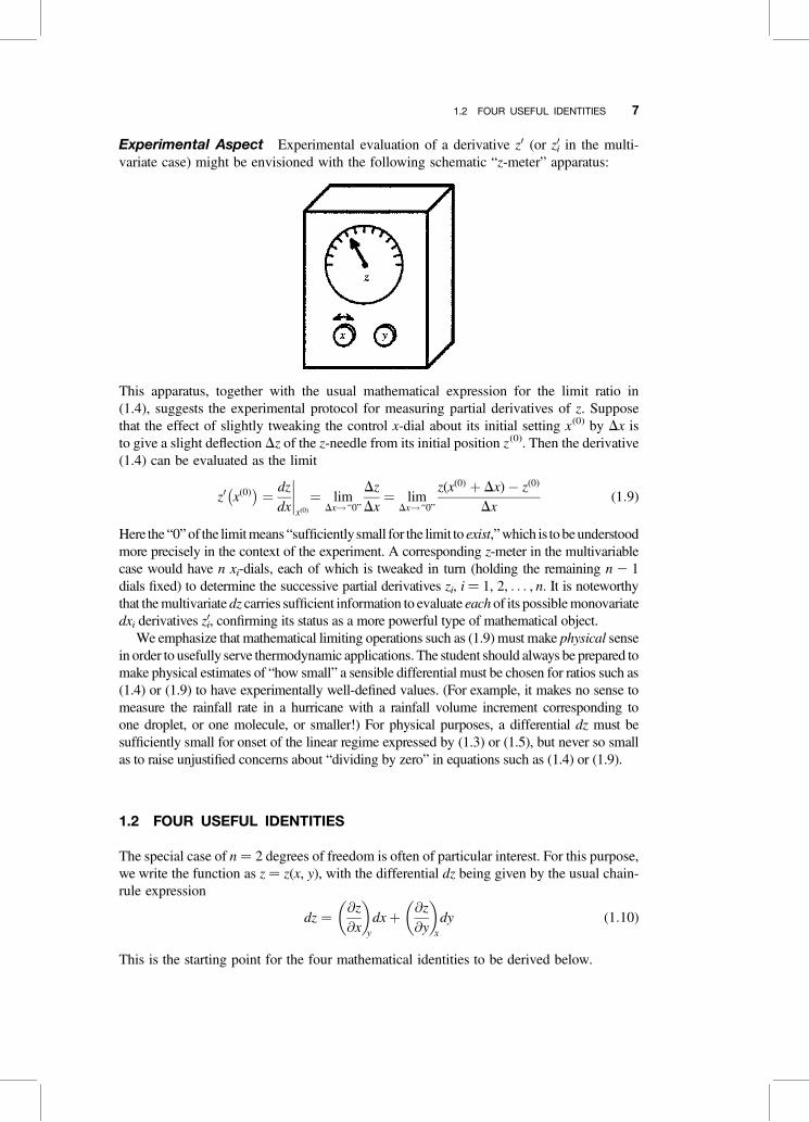
Experimental Aspect Experimental evaluation of a derivative z0 (or z0i in the multi-variate case) might be envisioned with the following schematic “z-meter” apparatus:

This apparatus, together with the usual mathematical expression for the limit ratio in(1.4), suggests the experimental protocol for measuring partial derivatives of z. Supposethat the effect of slightly tweaking the control x-dial about its initial setting x(0) by Dx isto give a slight deflection Dz of the z-needle from its initial position z(0). Then the derivative(1.4) can be evaluated as the limit

z0 x(0)� �

¼ dz

dx

��x(0)

¼ limDx!“0”

Dz

Dx¼ lim

Dx!“0”

z(x(0) þ Dx)� z(0)

Dx(1:9)

Here the “0” of the limit means “sufficientlysmall for the limit to exist,” which is to be understoodmore precisely in the context of the experiment. A corresponding z-meter in the multivariablecase would have n xi-dials, each of which is tweaked in turn (holding the remaining n 2 1dials fixed) to determine the successive partial derivatives zi, i ¼ 1, 2, . . . , n. It is noteworthythat the multivariate dz carries sufficient information to evaluate each of its possible monovariatedxi derivatives z0i, confirming its status as a more powerful type of mathematical object.

We emphasize that mathematical limiting operations such as (1.9) must make physical sensein order to usefully serve thermodynamic applications. The student should always be prepared tomake physical estimates of “how small” a sensible differential must be chosen for ratios such as(1.4) or (1.9) to have experimentally well-defined values. (For example, it makes no sense tomeasure the rainfall rate in a hurricane with a rainfall volume increment corresponding toone droplet, or one molecule, or smaller!) For physical purposes, a differential dz must besufficiently small for onset of the linear regime expressed by (1.3) or (1.5), but never so smallas to raise unjustified concerns about “dividing by zero” in equations such as (1.4) or (1.9).

1.2 FOUR USEFUL IDENTITIES

The special case of n ¼ 2 degrees of freedom is often of particular interest. For this purpose,we write the function as z ¼ z(x, y), with the differential dz being given by the usual chain-rule expression

dz ¼ @z

@x

� �y

dxþ @z

@y

� �x

dy (1:10)

This is the starting point for the four mathematical identities to be derived below.

1.2 FOUR USEFUL IDENTITIES 7

(i) Reduction to n 5 1 (Single Degree of Freedom) Suppose that the “indepen-dent” variables x ¼ x(u), y ¼ y(u) are both simple functions of a single variable u, sothat z ¼ z(u) has only “ordinary” derivative dependence on u. What is dz/du? To obtainthis ratio, we can simply divide dz (1.10) by du to obtain

dz

du¼ @z

@x

� �y

dx

duþ @z

@y

� �x

dy

du(1:11)

Note closely the distinctions between ordinary (d ) and partial (@) derivatives throughoutthis formula.

Note also that we employ “physicist’s notation” for functions, in which both z ¼ z(u)and z ¼ z(x, y) express how z depends on the variables specified in parentheses (eventhough the mathematical formulas that express this dependence might be quite differentin the two cases). Although somewhat “unmathematical,” the chosen notation betterexpresses the experimental relationship (1.1), in which control variables xi might bechosen for convenience in many ways, but the target property z is independent of thischoice. For example, the volume of a sphere could be equivalently expressed in terms ofits measured diameter [V ¼ V(d ) ¼ pd3/6] or surface area [V ¼ V(A) ¼ (p1/2/6)A3/2],despite the fact that the mathematical dependence (i.e., whether there is a cubic or three-halves power in the chosen measurement argument) is different in the two cases.

(ii) Change of Differentiated Variable Suppose that we re-express z ¼ z(x, u) as afunction of x and a new variable u, where the “old” variable y ¼ y(x, u) is also expressiblein the new independent variables (x, u). To find the expression for (@z/@u)x from the “old”differential expression (1.10), we merely divide (1.10) throughout by “du at constant x”[replacing the constrained ratio “dz/du at constant x” on the left-hand side by the properpartial derivative notation, (@z/@u)x, and similarly for both ratios on the right-hand side]:

@z

@u

� �x

¼ @z

@x

� �y

@x

@u

� �x

þ @z

@y

� �x

@y

@u

� �x

However, the partial derivative (@x/@u)x ¼ 0 (because, at constant x, derivatives of x withrespect to anything must vanish). The above equation thereby simplifies to

@z

@u

� �x

¼ @z

@y

� �x

@y

@u

� �x

(1:12)

Note how the right-hand side has the proper “balance” of differential terms, as though dycan be cancelled from numerator and denominator to give the desired partial derivative.

(iii) Change of Variable Held Constant Under the same change of variables(x, y) ! (x, u), we can also obtain the partial derivative (@z/@x)u (with the new variableu held constant). Starting again from (1.10), we “divide by dx at constant u” on bothsides (using proper partial derivative notation for the constrained ratios) to obtain

@z

@x

� �u

¼ @z

@x

� �y

@x

@x

� �u

þ @z

@y

� �x

@y

@x

� �u


But (@x/@x)u ¼ 1 (since the variations of x with itself are unity, no matter what else is con-stant), so the equation becomes

@z

@x

� �u

¼ @z

@x

� �y

þ @z

@y

� �x

@y

@x

� �u

(1:13)

Note that this identity clearly shows that (@z/@x)y = (@z/@x)u, i.e., that the variable heldconstant matters in these derivatives! (Strictly speaking, a lazy notation such as “@z/@x”has no meaning whatsoever!) Although the inconvenient notation of partial derivativesmakes it somewhat tedious to keep the inactive (constant) “background” variables inmind, it is important from a physical and pedagogical standpoint that this be done as care-fully as possible. (The tedium of this notation is avoided in the geometrical thermody-namics to be presented in Part III.)

SIDEBAR 1.3: CHANGE-OF-VARIABLE EXERCISE

Exercise Suppose the rectangular area A in Sidebar 1.1 is expressed in terms of side x andperimeter P. What are (@A/@P)x and (@A/@x)P?

Solution The new and old variables are related by P ¼ 2(x þ y), or

y ¼ 12 P� x

so that

@y

@x

� �P

¼ �1,@y

@P

� �x

¼ 12

From the identity (1.12), we obtain

@A

@P

� �x

¼ @A

@y

� �x

@y

@P

� �x

¼ (x)12

� �¼ 1

2 x

Similarly, from the identity (1.13), we obtain

@A

@x

� �P

¼ @A

@x

� �y

þ @A

@y

� �x

@y

@x

� �P

¼ yþ (x)(�1) ¼ 12 P� 2x

[Of course, in this case, it is also possible to solve explicitly for A ¼ A(x, P) ¼ 12Px2x2 and

differentiate directly, but this “direct” route is often less practical than use of the identities(1.12), (1.13).]

(iv) Jacobi (Cyclic) Identity A provocative identity of great generality and usefulnessfor n ¼ 2 is obtained by considering (1.10) under conditions of constant z (i.e., dz ¼ 0). Ifwe then “divide by dx at constant z” (making the usual change of notation from ratio to

1.2 FOUR USEFUL IDENTITIES 9

partial derivative), we obtain

0 ¼ @z

@x

� �y

þ @z

@y

� �x

@y

@x

� �z

Noting that (@z/@x)y ¼ 1/(@x/@z)y, we can rewrite the above equation as

@x

@y

� �z

@z

@x

� �y

@y

@z

� �x

¼ �1 (1:14a)

Alternately, we can rewrite this identity as

@x

@y

� �z

¼ � @z=@yð Þx(@z=@x)y

(1:14b)

As one can see in (1.14a), the variables (x, y, z) are “cycled” in the three derivatives, eachappearing once in the numerator, once in the denominator, and once as the constantvariable. The cyclic symmetry makes it easy (and advisable) to commit this identity tomemory, even if it can be easily rederived from (1.10) for use as needed.

The identities (1.11)–(1.14) are among the most commonly employed in thermody-namic derivations, because two degrees of freedom underlie the important special caseof “simple” substances (pure, homogeneous), as will be subsequently described.

1.3 EXACT AND INEXACT DIFFERENTIALS

While the existence of a functional relationship z ¼ z(x1, x2, . . . , xn) allows its differentialdz to be unambiguously determined, the reverse need not be the case. Differentials dz forwhich no corresponding function z exists are called inexact (or “imperfect,” often markedwith a slash: d�), whereas those for which z exists are exact (or “perfect”). The basic distinc-tion between exact (d-type) and inexact (d�-type) differentials lies at the heart of thermodyn-amic usage of the differential concept, so we must understand clearly how the two cases canbe mathematically distinguished. Differentials of heat, for example, are found to belong tothe “imperfect” category, whereas those of energy are “perfect.”

It might seem that a suitable z (up to an arbitrary constant) could always be generatedfrom a given differential form dz by merely evaluating the integral

z ¼?ð

dz

This is indeed always possible for a single variable n ¼ 1 (ordinary calculus), where thedistinction between exact and inexact differentials disappears. However, for n . 1, it isclear that integrals over dz must generally depend on the chosen path along which the inte-gration is performed. Integrals of multivariate differentials are called line integrals (or pathintegrals) to indicate this distinction from ordinary (monovariate) integrals. For inexact d�z,the line integral

Ðd�z is path-dependent (and therefore not uniquely defined), the signature


defect of inexactness. Only in the case of an exact differential dz does the indefinite integralÐdz evaluate to a unique function z, independent of the chosen integration path.

Let us first consider this issue in the simple case n ¼ 2, with independent variables x, yand dependent variable z. If a well-defined function z(x, y) exists, then dz [of the form(1.10)] is certainly exact. Furthermore, if we evaluate the definite integral from initial(x1, y1) to final (x2, y2), the result is simply

I ¼ðx2,y2

x1,y1

dz ¼ z x2, y2ð Þ � z x1, y1ð Þ (1:15)

The important point is that the final value of the integral depends only on the two endpoints,i.e., the value of the function z at (x1, y1) and (x2, y2), but not the chosen path of integration(as illustrated in Sidebar 1.4). Moreover, in the special case of a cyclic integral (denoted

Þ),

where “initial” and “final” limits coincide, the integral (1.15) necessarily vanishes for anexact differential, independent of how the cyclic path is chosen. We can therefore statethe following integral criterion for exactness:

Integral criterion: The differential dz is exact if and only ifÞdz ¼ 0 for all possible paths

(1:16a)

A closely related criterion can be stated in graphical terms:

Graphical criterion: The differential dz is exact if and only if its integral

z(x, y) ¼Ð

dz is graphable(1:16b)

This criterion is rather self-evident, because the condition that z ¼ z(x, y) be “graphable” ismerely that a unique z-value be given any chosen x, y, i.e., that z ¼ z(x, y) satisfies therequirements of a function. However, both criteria require global (integral) informationthat may be difficult to obtain from local measurements.

SIDEBAR 1.4: SUMMIT TRAIL PROBLEM

Problem On the coast of Hawaii, a sign points to a distant volcano with the information,“Summit: distance ¼ 15.3 km, altitude ¼ 4.2 km.” How can one determine which (if either)of the differential quantities dl (distance) or dh (altitude) is exact?

Solution By measuring (e.g., with ruler and altimeter) the differential changes dl, dh andintegrating (summing up) their cumulative changes Il, Ih from coast to summit,

Il ¼ðsummit

coast

dl, Ih ¼ðsummit

coast

dh

one could verify experimentally that Ih is independent of the path chosen to the summit, sothat dh is exact, whereas Il is path-dependent, so that d�l is inexact by (1.16a).

1.3 EXACT AND INEXACT DIFFERENTIALS 11

As an alternative strategy, one might ask in a local bookshop for an “altitude map” and a“distance map” for Hawaii. A mathematically savvy shopkeeper may reply that the first (a“topo map”) is readily available, because altitude is easily graphable in topographic form,whereas the second is not, because distance is inherently a path-dependent, ungraphablequantity. This reply points, by (1.16b), to the same conclusion.

A more convenient differential criterion for exactness was established by Euler. Supposethat the differential dz consists as usual of contributions from dx and dy variations,

dz ¼ M(x, y) dxþ N(x, y) dy

where the respective coefficients M ¼ M(x, y) and N ¼ N(x, y) are stipulated functions ofx and y. We can then state the Euler criterion as follows:

Euler criterion (n¼ 2): The differential dz¼M dxþN dy is exact if and only if

@M

@y

� �x

¼ @N

@x

� �y

at every point x, y(1:17)

It is easy to recognize that the Euler criterion will be satisfied if the integral or graphicalcriteria (1.16) are satisfied. Suppose that z(x, y) indeed exists (e.g., displayed as a graph), sothat (1.10) is assured. Comparison of (1.10) with the assumed form of the differential thenshows that

M(x, y) ¼ @z

@x

� �y

, N(x, y) ¼ @z

@y

� �x

(1:18)

The M-derivative of the Euler criterion (1.17) can therefore be evaluated as

@M

@y

� �x

¼ @

@y

@z

@x

� �y

!x

¼ @2z

@y @x(1:19a)

whereas the N-derivative is similarly

@N

@x

� �y

¼ @

@x

@z

@y

� �x

� �y

¼ @2z

@x @y(1:19b)

The Euler criterion is therefore equivalent to the familiar “mixed partials of a function areequal” rule of calculus. This cross-differentiation rule is also the condition for the functionz(x, y) to have well-defined (single-valued) first derivatives at each point, and thus to begraphable.


SIDEBAR 1.5: EXACT DIFFERENTIAL EXERCISES

Exercises Use the Euler criterion (1.17) to determine whether each of the followingdifferentials dz is exact or inexact:

(a) dz ¼ y dxþ x dy

(b) dz ¼ y2 dxþ xy dy

(c) dz ¼ ( y=x) dxþ ln(x) dy

(d) dz ¼ 2x�1=3y7(y dxþ 12x dy)

Solutions (a) exact; (b) inexact; (c) exact; (d) exact. To work out the solution of (d) inmore detail, we note that

M ¼ 2x�1=3y8, N ¼ 24x2=3y7

so that

@M

@y

� �x

¼ 16x�1=3y7 ¼ @N

@x

� �y

as required for exactness.

SIDEBAR 1.6: ILLUSTRATIVE LINE INTEGRALS

Let us examine the line integrals of two simple inexact differentials, namely,

d�z1 ¼ y dx, d�z2 ¼ x dy (S1:6-1)

to see their explicit path dependence. We employ the path y ¼ y(x) shown in figurepanel (a) to connect the initial point P ¼ (x1, y1) to the final point Q ¼ (x2, y2) in thedefinite integrals

I1 ¼ðQP

d�z1 ¼ðQP

y dx, I2 ¼ðQP

d�z2 ¼ðQP

x dy (S1:6-2)

The first integral I1 is just the area under the curve y ¼ y(x), as shown by the shadedregion in panel (b). Similarly, the second integral I2 is the area to the left of thiscurve, as shown by the shaded region in panel (c). Clearly, the values of both I1

and I2 are dependent on the chosen path of integration, confirming that d�z1 and d�z2

are inexact. However, the sum of these differentials, dz¼ d�z1 þ d�z2 ¼ y dxþ x dy, isevidently exact [cf. part (a) of Sidebar 1.5]. By inspection, its integral

I ¼ðQP

dz ¼ I1 þ I2 (S1:6-3)

is the total area of the shaded L-shaped region in panel (d), which depends on theendpoints (x1, y1), (x2, y2) but not the connecting path.

1.3 EXACT AND INEXACT DIFFERENTIALS 13

For arbitrary n, the more general statement of the Euler criterion can be formulated interms of a general n-term differential form

dz ¼Xn

i¼1

Ridxi (1:20)

with coefficients Ri ¼ Ri(x1, x2, . . . , xn). The generalization of (1.17) is

Euler criterion (general n): The differential dz¼ R1 dx1þR2 dx2þ � � � þRn dxn (1:21)

is exact if and only if@Ri

@xj

� �x

¼ @Rj

@xi

� �x

for all i, j¼ 1, 2, . . . , n

(i.e., mixed partial derivatives are equal for any chosen pair of variables xi, xj):

This fundamental relation underlies all thermodynamic descriptions of exact (conserved)differential quantities such as internal energy or entropy, as will be shown in subsequentchapters.


Finally, we briefly mention the concept of an integrating factor, a multiplicative factor(L) that converts an inexact differential (d�f ) to an exact differential (dg), namely,

Ld�f ¼ dg (1:22)

Integrating factors L may or may not exist for a given d�f, and if they exist, they are generallynon-unique (e.g., L0 ¼ cL is also an integrating factor for any constant c). In simple cases,an integrating factor can be guessed “by inspection”; for example, it is easy to see that L ¼1/y is an integrating factor for the inexact differential in Sidebar 1.5(b). In more complexcases, the Euler condition (1.21) can be used to convert (1.22) into a differential equationfor determining L. In the thermodynamic context, however, the most important integratingfactor is that for the differential of heat, and this factor (namely, L ¼ 1/T, the inverse temp-erature) will be obtained from physical considerations, rather than, for example, by solvinga differential equation.

1.4 TAYLOR SERIES

A common situation in thermodynamics is that some property z(x) and its lower derivatives(z0, z00, z000, . . .) have been measured at a certain point x0, and one wishes to use this infor-mation to approximate the behavior of the function z(x0 þ Dx) in the Dx-neighborhood ofx0. For this purpose, the fundamental Taylor series (or MacLaurin series, the special casefor x0 ¼ 0) yields approximations that are useful for sufficiently small Dx:

z(x0 þ Dx) ’ z(x0)þ z0(x0)Dxþ 12!

z00(x0)(Dx)2 þ 13!

z000(x0)(Dx)3 þ � � � (1:23)

The student of thermodynamics should be able to generate such Taylor series expansionsfor common algebraic and trigonometric functions.

SIDEBAR 1.7: TAYLOR SERIES EXERCISES

Exercises Use the first few terms of the Taylor series expansion (1.23) to develop small-xapproximations for the functions

(a) z(x) ¼ (1� x)�1

(b) z(x) ¼ ln(1þ x)

(c) z(x) ¼ [cos(x)]�1=2

(d) z(x) ¼ (1þ x2)1=2

Solutions

(a) (1� x)�1 ’ 1þ xþ x2 þ x3 þ � � �(b) ln(1þ x) ’ x� x2=2þ x3=3� � � �(c) [cos (x)]�1=2 ’ 1þ x2=4þ 7x4=96þ � � �(d) (1þ x2)1=2 ’ 1þ x2=2� x4=8þ � � �

1.4 TAYLOR SERIES 15

PART I INDUCTIVE FOUNDATIONS OF CLASSICAL THERMODYNAMICS

Documents

Transcript of PART I INDUCTIVE FOUNDATIONS OF CLASSICAL THERMODYNAMICS