PART FOUR

ESTIMATING COMMUNITY PARAMETERS

Community ecologists face a special set of statistical problems in attempting to

characterize and measure the properties of communities of plants and animals.

Some community studies, such as energetic analyses, need only apply the general

principles discussed in Part I to estimate the abundances of the many species that

comprise the community. But other community studies need to utilize new

parameters applicable only at the community level. One community parameter is

similarity, and Chapter 12 discusses how to measure the similarity between

communities. Similarity is the basis of classification, and this chapter discusses

cluster analysis as one method of objectively defining the relationships among many

community samples.

Plant ecologists in particular have developed a wide array of multivariate

statistical techniques to assist in the analysis of community patterns and to help in

defining the environmental controls of community patterns. Gradient analysis and

ordination techniques are part of the statistical tool-kit of all community ecologists.

Although these methods are briefly mentioned in Chapter 11, I do not treat them in

this book because there are several good texts devoted specifically to multivariate

statistical methods in ecology (Pielou 1984, Digby and Kempton 1987).

Species diversity is one of the most obvious and characteristic feature of a

community. From the earliest observations about the rich diversity of tropical

communities in comparison with impoverished polar communities, ecologists have

tried to quantify the diversity concept. Chapter 13 summarizes the accumulated

wisdom of ways to measure biological diversity in plant and animal communities.

Chapter 12 Page 480

Niche theory has been one of the most powerful methods for analyzing

community structure after the pioneering work of MacArthur (1968). Analyses of the

structure of a community and the dynamic interactions of competing species all

depend on the measurement of the niche parameters of species. Chapter 14

presents the methods developed for the measurement of niche breadth and niche

overlap in natural communities. The measurement of dietary preference is similar to

the problem of measuring niche breadth, and Chapter 13 discusses the measures

that have been suggested for quantifying the simple idea of preference in animals.

Other community concepts such as trophic structure and succession are

analyzed by various combinations of the methods outlined in the earlier parts of this

book.

Community dynamics is an important area of analysis in modern ecology and a

challenging focus of experimental work. To study communities rigorously, ecologists

must use a wide array of population and community methods, all arranged in an

experimental design that will satisfy a pure statistician. To achieve this goal is

perhaps the most challenging methodological problems in modern ecology.

CHAPTER 12

SIMILARITY COEFFICIENTS AND CLUSTER ANALYSIS

(Version 5, 14 March 2014) Page

12.1 MEASUREMENT OF SIMILARITY ................................................................ 486 12.1.1 Binary Similarity Coefficients ........................................................... 487

12.1.2 Distance Coefficients ....................................................................... 492

12.1.3 Correlation Coefficients ................................................................... 502 12.1.4 Other Similarity Measures ............................................................... 503

12.2 DATA STANDARDIZATION ........................................................................... 508

12.3 CLUSTER ANALYSIS .................................................................................... 513

12.3.1 Single Linkage Clustering ................................................................. 514 12.3.2 Complete Linkage Clustering ........................................................... 518 12.3.3 Average Linkage Clustering ............................................................. 520

12.4 RECOMMENDATIONS FOR CLASSIFICATIONS ......................................... 523

12.5 OTHER MULTIVARIATE TECHNIQUES ........................................................ 525

12.6 SUMMARY ...................................................................................................... 525

SELECTED REFERENCES .................................................................................... 526

QUESTIONS AND PROBLEMS ............................................................................. 527

In many community studies ecologists obtain a list of the species that occur in each of

several communities, and, if quantitative sampling has been done, some measure of

the relative abundance of each species. Often the purpose of this sampling is to

determine if the communities can be classified together or need to be separated. For

the designation of conservation areas we will often wish to ask how much separate

areas differ in their flora and fauna. As a start to answering these complex questions

of community classification, we now ask how we can measure the similarity between

two such community samples.

Chapter 12 Page 486

12.1 MEASUREMENT OF SIMILARITY

There are more than two dozen measures of similarity available (Legendre and

Legendre 1983, Wolda 1981, Koleff et al. 2003) and much confusion exists about

which measure to use. Similarity measures are peculiar kinds of coefficients because

they are mainly descriptive coefficients, not estimators of some statistical parameter.

It is difficult to give reliable confidence intervals for most measures of similarity and

probable errors can be estimated only by some type of randomization procedure

(Ricklefs and Lau 1980; see Chapter 15, page 000).

There are two broad classes of similarity measures. Binary similarity coefficients

are used when only presence/absence data are available for the species in a

community, and are thus appropriate for the nominal scale of measurement.

Quantitative similarity coefficients require that some measure of relative abundance

also be available for each species. Relative abundance may be measured by number

of individuals, biomass, cover, productivity, or any measure that quantifies the

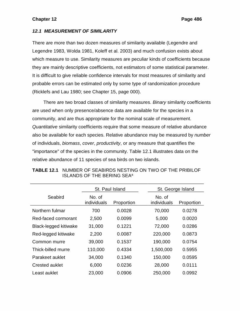
"importance" of the species in the community. Table 12.1 illustrates data on the

relative abundance of 11 species of sea birds on two islands.

TABLE 12.1 NUMBER OF SEABIRDS NESTING ON TWO OF THE PRIBILOF ISLANDS OF THE BERING SEAa

St. Paul Island St. George Island

Seabird No. of individuals

Proportion

No. of individuals

Proportion

Northern fulmar 700 0.0028 70,000 0.0278 Red-faced cormorant 2,500 0.0099 5,000 0.0020 Black-legged kitiwake 31,000 0.1221 72,000 0.0286 Red-legged kitiwake 2,200 0.0087 220,000 0.0873 Common murre 39,000 0.1537 190,000 0.0754 Thick-billed murre 110,000 0.4334 1,500,000 0.5955 Parakeet auklet 34,000 0.1340 150,000 0.0595 Crested auklet 6,000 0.0236 28,000 0.0111 Least auklet 23,000 0.0906 250,000 0.0992

Chapter 12 Page 487

Horned puffin 4,400 0.0173 28,000 0.0111 Tufted puffin 1,000 0.0039 6,000 0.0024

Total 253,800 1.0000 2,519,000 0.9999 a Data from Hunt et al., 1986.

There are two desirable attributes of all similarity measures. First, the measure

should be independent of sample size and of the number of species in the community

(Wolda 1981). Second, the measure should increase smoothly from some fixed

minimum to a fixed maximum, as the two community samples become more similar.

Wolda (1981), Colwell and Coddington (1994), and Chao et al.(2006) have done an

extensive analysis of the properties of similarity coefficients to see if they all behave

desirably, and their work forms the basis of many of the recommendations I give here.

12.1.1 Binary Similarity Coefficients

The simplest similarity measures deal only with presence-absence data. The basic

data for calculating binary (or association) coefficients is a 2x2 table:

Sample A No. of species

present No. of species

absent

Sample B No. of species present a b

No. of species absent c d

where:

Number of species in sample A and sample B (joint occurences) Number of species in sample B but not in sample A Number of species in sample A but not in sample B Number of species absent

abcd

==== in both samples (zero-zero matches)

There is considerable disagreement in the literature about whether d is a biologically

meaningful number. It could be meaningful in an area where the flora or fauna is well

known and the absence of certain species is relevant. But at the other extreme,

elephants are always absent from plankton samples and clearly they should not be

included in d when plankton are being studied. For this reason most users of similarity

measures ignore species that are absent in both samples.

Chapter 12 Page 488

There are more than 20 binary similarity measures now in the literature

(Cheetham and Hazel 1969) and they have been reviewed by Clifford and

Stephenson (1975, Chapter 6) and by Romesburg (1984, Chapter 10). I will describe

here only two of the most often used similarity coefficients for binary data.

Jaccard’s Index:

jaS

a b c=

+ + (12.1)

where:

Jaccard's similarity coefficient, , As defined above in presence-absence matrix

jSa b c

==

This index can be modified to a coefficient of dissimilarity by taking its inverse:

Jaccard's dissimilarity coefficient 1 jS= − (12.2)

Sorensen’s Index: This measure is very similar to the Jaccard measure, and was

first used by Czekanowski in 1913 and discovered anew by Sorensen (1948):

22S

aSa b c

=+ +

(12.3)

where SS = Sorensen’s similarity coefficient

This index can also be modified to a coefficient of dissimilarity by taking its inverse:

Sorensen's dissimilarity coefficient 1 sS= − (12.4)

This coefficient weights matches in species composition between the two samples

more heavily than mismatches. Whether or not one thinks this weighting is desirable

will depend on the quality of the data. If many species are present in a community but

not present in a sample from that community, it may be useful to use Sorensen's

coefficient rather than Jaccard's. But the Sorensen and Jaccard coefficients are very

closely correlated (Baselga 2012, Figure 4).

Simple Matching Coefficient: This is the simplest coefficient for binary data that

makes use of negative matches as well as positive matches. It is not used very

Chapter 12 Page 489

frequently because for most data sets negative matches are not biologically

meaningful.

SMa dS

a b c d+

=+ + +

(12.5)

where SSM = Simple matching similarity coefficient

Baroni-Urbani and Buser Coefficient: This is a more complex similarity coefficient

that also makes use of negative matches.

Bad aS

a b c ad+

=+ + +

(12.6)

where SB = Baroni-Urbani and Buser similarity coefficient

This was proposed by Baroni-Urbani and Buser (1976). Faith (1983) proposed a very

similar binary similarity index. Both these coefficients can also be turned into

dissimilarity measures by taking their inverse (as above).

The range of all similarity coefficients for binary data is supposed to be 0 (no

similarity) to 1.0 (complete similarity). In fact, this is not true for all coefficients. Wolda

(1981) investigated how sample size and species richness affected the maximum

value that could be obtained with similarity coefficients. He used a simulated

community of known species richness with 100,000 individuals whose species

abundances were distributed according to the log series (see Krebs 2009 Chapter

23). Figure 12.1 shows how the coefficient of Sorensen and the Baroni-Urbani

coefficient are affected by sample size and by species richness. Sample size effects

are very large indeed. For example, the maximum value of the Sorensen coefficient

when 750 species are present in the community and each community sample

contains 200 individuals is 0.55 not 1.0 as one might expect.

Chapter 12 Page 490

Higher diversity(750 species)

Size of smaller sample100 200 500 1000 5000

Sim

ilarit

y Co

effic

ient

0.0

0.2

0.4

0.6

0.8

1.0

Lower diversity(150 species)

Size of smaller sample100 200 500 1000 5000

0.0

0.2

0.4

0.6

0.8

1.0

Size of smaller sample100 200 500 1000 5000

Sim

ilarit

y Co

effic

ient

0.0

0.2

0.4

0.6

0.8

1.0

Size of smaller sample100 200 500 1000 5000

0.0

0.2

0.4

0.6

0.8

1.0

50005000

5000 5000

1000 1000

1000 1000

Baroni-Urbanicoefficient

Sorensencoefficient

Figure 12.1 Expected maximum values of two commonly used binary coefficients of similarity as a function of sample size. The number of individuals in the smaller of the two community samples is given on the X axis, and the lines connect samples of equal size for the larger community sample (n = 5000 (black), 1000 (red), 500 (green), and 200 (yellow); a different symbol is used for each of these sample sizes). A highly diverse community is shown on the left and a lower-diversity community on the right. Although the theoretical maximum value of each of these coefficients is 1.0, the expected maximum is much less than 1.0 when samples are small. (From Wolda, 1981.)

Wolda (1981) did not investigate the sampling properties of the Jaccard

coefficient, but they would probably be similar to those for the Sorensen coefficient

(Fig. 12.1). Wolda (1981) showed graphically that there were similar sampling

problems with almost all the available measures of similarity, and this has led to an

attempt to reformulate similarity measures to circumvent the bias problems illustrated

in Figure 12.1 from samples of different sizes.

Chapter 12 Page 491

Binary similarity coefficients are crude measures available for judging similarity

between communities because they do not take commonness and scarcity into

consideration. Binary coefficients thus weight rare species the same as common

species, and should be used whenever one wishes to weight all species on an equal

footing. More commonly, binary similarity measures are used because only lists of

species names are available for particular communities and comparisons are possible

only at this lower level of resolution.

Box 12.1 CALCULATION OF TRADITIONAL SIMILARITY MEASURES FOR BINARY DATA

The crustacean zooplankton of the Great Lakes were sampled by Watson (1974), who obtained these data:

Lake Erie No. of species

present No. of species

absent

Lake Ontario No. of species present 18 1

No. of species absent 1 5

A total of 25 species of crustacean zooplankton occur in all the Great Lakes, and of these 5 species do not occur in either Lake Erie or Lake Ontario. Jaccard’s Index:

18 0.9018 + 1 + 1

JaS

a b c=

+ +

= =

Sorensen’s Index: 2

22(18) 0.95

2(18) + 1 + 1

SaS

a b c=

+ +

= =

Simple matching coefficient:

18 5 0.9218 1 1 5

SMa dS

a b c d+

=+ + +

+= =

+ + +

Baroni-Urbani and Buser coefficient:

Chapter 12 Page 492

( )( )( )( )

18 5 + 18 27.487 0.9329.48718 1 1 18 5

Bad aS

a b c ad+

=+ + +

= = =+ + +

The unsatisfactory performance of all binary similarity indices has led to a

reformulation of their calculation by Chao et al. (2005, 2006). The problem lies in

species that are shared species between the two samples but are not seen in the

sampling. Figure 12.2 illustrates the problem of shared species in two quadrats. By

reformulating these data in a probabilistic format Chao et al. (2006) were able to bring

together indices based on presence-absence data and indices based on relative

abundance or biomass. Table 12.2 gives the reformulation for the Jaccard and the

Sorensen indices.

The first step is to redefine the traditional binary counts as follows:

1

2

12

12

1 12

2 12

total number of species in sample 1 total number of species in sample 2 number of species present in both samples

SSSa Sb S Sc S S

===

== −= −

Table 12.2 REFORMULATION OF THE JACCARD AND SORENSEN INDICES FOR PRESENCE-ABSENCE DATA AND ABUNDANCE DATA. (From Chao et al. 2006). Index Presence/absence

based with a, b, c

Presence/absence based

with S1, S2, S12

Abundance based

(see definitions below)

Jaccard aa b c+ +

12

1 2 12

SS S S+ −

UV

U V UV+ −

Sorensen ( )

22

aa b c+ +

12

1 2

2SS S+

2UVU V+

Chapter 12 Page 493

Case 1

Case 1

Species from sample 2Is shared

Species fromsample 1Is shared

Sample 1

Sample 2

Case 1

Case 2

Species from sample 2Is not shared

Sample 1

Sample 2

Case 1

Case 3

Species fromsample 1

Is not shared

Sample 1

Sample 2

Case 1

Case 4

Sample 1

Sample 2

Figure 12.2 A schematic illustration of the meaning of shared species for two community samples. Sample 1 is green, Sample 2 is pink. The green dots represent a species selected at random from sample 1, and the red dots represent a species selected at random from sample 2. In Case 1 both species are shared species (i.e. they occur in both samples). In Case 2 the species chosen at random from sample 1 is a shared species but the species chosen at random from sample 2 is not a shared species. The reverse is true for Case 3. In Case 4 neither of the chosen species is a shared species. (Modified from Chao et al. 2006).

Then Chao et al. (1986) generalized these variables to include abundance data rather

than just presence-absence data as follows:

total relative abundances of the shared species in sample 1 total relative abundances of the shared species in sample 2

where:count or biomass in sample relative abundance

total count or biomass

UV

x

==

= in sample x

Chapter 12 Page 494

Note that for the definition of U and V we use only the shared species in the two

samples. We now have reformulated the Jaccard and Sorensen indices to include

quantitative data on abundance, as shown in Table 12.2.

The problem now is that both U and V are negatively biased because of the

missed shared species. Chao et al. (2006) derived sample estimates of U and V that

corrects for unseen shared species, and these sample estimates can then be used in

the calculations in Table 12.2.

( ) ( )( ) ( )

1

1 12

1

1 12

1ˆ 12

1ˆ 12

a ai i

ii ia a

i ii

i i

mX f XU I Yn m f n

nY f YV I Xm n f m

+

= =+

+

= =+

−= + =

−= + =

∑ ∑

∑ ∑ (12.7)

where

number of shared species between samples 1 and 2 number of individuals (or biomass) of species in sample 1 total number of individuals (or biomass) in sample 1 total number of individuals

i

aX inm

====

1

2

(or biomass) in sample 2 observed number of the shared species that occur once in sample 1 observed number of shared species that occur twice in sample 1 indicator function ( 1 if the expre

ff

I I

+

+

=== =

1

2

ssion is true, 0 if false) number of individuals (or biomass) of species in sample 2 observed number of the shared species that occur once in sample 2 observed number of shared species

i

IY iff+

+

==== that occur twice in sample 2

The first term in these equations gives the original unadjusted estimator for the

similarity function and the second term corrects the estimator for the number of

unseen shared species.

The recommendation of Chao et al. (2006) is to use these adjusted estimates of

U and V in the formulas in eq. (12.7) in Table 12.2 to calculate the adjusted Jaccard

and adjusted Sorensen indices for abundance data.

ˆ ˆAdjusted Jaccard index of similarity ˆ ˆ ˆ ˆ

UVU V UV

=+ −

(12.8)

ˆ ˆ2Adjusted Sorensen index of similarity ˆ ˆUV

U V=

+ (12.9)

Chapter 12 Page 495

where U and V are as defined in equation (12.7) above

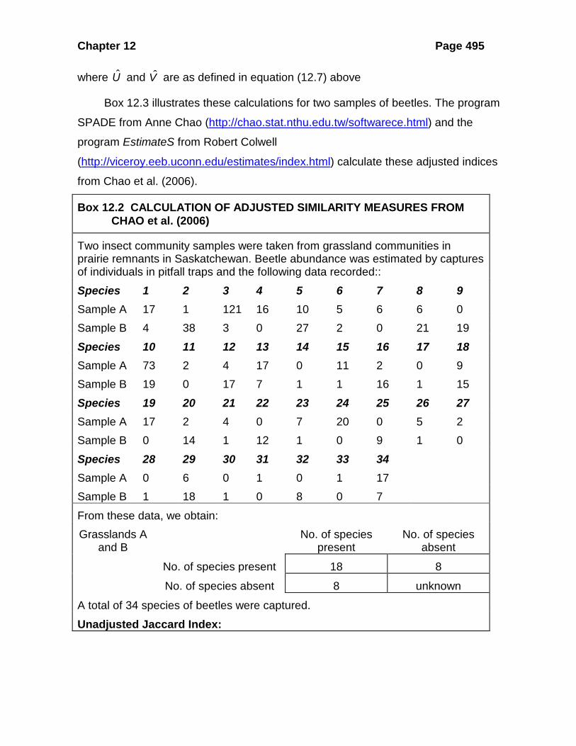
Box 12.3 illustrates these calculations for two samples of beetles. The program

SPADE from Anne Chao (http://chao.stat.nthu.edu.tw/softwarece.html) and the

program EstimateS from Robert Colwell

(http://viceroy.eeb.uconn.edu/estimates/index.html) calculate these adjusted indices

from Chao et al. (2006).

Box 12.2 CALCULATION OF ADJUSTED SIMILARITY MEASURES FROM CHAO et al. (2006)

Two insect community samples were taken from grassland communities in prairie remnants in Saskatchewan. Beetle abundance was estimated by captures of individuals in pitfall traps and the following data recorded:: Species 1 2 3 4 5 6 7 8 9 Sample A 17 1 121 16 10 5 6 6 0 Sample B 4 38 3 0 27 2 0 21 19 Species 10 11 12 13 14 15 16 17 18 Sample A 73 2 4 17 0 11 2 0 9 Sample B 19 0 17 7 1 1 16 1 15 Species 19 20 21 22 23 24 25 26 27 Sample A 17 2 4 0 7 20 0 5 2 Sample B 0 14 1 12 1 0 9 1 0 Species 28 29 30 31 32 33 34 Sample A 0 6 0 1 0 1 17 Sample B 1 18 1 0 8 0 7 From these data, we obtain: Grasslands A

and B No. of species

present No. of species

absent

No. of species present 18 8

No. of species absent 8 unknown

A total of 34 species of beetles were captured. Unadjusted Jaccard Index:

Chapter 12 Page 496

18 0.529418 + 8 + 8

JaS

a b c=

+ +

= =

Unadjusted Sorensen Index: 2

22(18) 0.6923

2(18) + 8 + 8

SaS

a b c=

+ +

= =

Sample estimates of U and V: (eq. 12.7) To calculate these estimates we require these parameters:

1

18 number of shared species between samples 1 and 2382 total number of individuals in sample 1264 total number of individuals in sample 24 observed number of the shared species that occur

anmf+

= == == == =

2

1

2

once in sample 11 observed number of shared species that occur twice in sample 11 observed number of the shared species that occur once in sample 22 observed number of shared species t

fff

+

+

+

= == == = hat occur twice in sample 2

( ) ( )

[ ]

1

1 12

1ˆ 12

0.8298 0.9962 * 2 * 0.07068 0.9707

a ai i

ii i

mX f XU I Yn m f n

+

= =+

−= + =

= + =

∑ ∑

( ) ( )

[ ]

1

1 12

1ˆ 12

0.8030 0.9974 * 0.25 * 0.1439 0.8389

a ai i

ii i

nY f YV I Xm n f m

+

= =+

−= + =

= + =

∑ ∑

Adjusted Jaccard and Sorensen abundance indices: From equation (12.8), the adjusted Jaccard abundance Index is given by:

( )0.9707 * 0.8389

0.9707 0.8389 0.9707 * 0.83890.8182

UVU V UV

=+ − + −

=

And the adjusted Sorensen abundance index is from equation (12.9): 2 2 * 0.9707 * 0.8389 0.9000

0.9707 0.8389UV

U V= =

+ +

Chapter 12 Page 497

12.1.2 Distance Coefficients

Distance coefficients are intuitively appealing to an ecologist because we can

visualize them. Note that distance coefficients are measures of dissimilarity, rather

than similarity. When a distance coefficient is zero, communities are identical. We can

visualize distance measures of similarity by considering the simplest case of two

species in two community samples. Distance coefficients typically require some

measure of abundance for each species in the community. Figure 12.3 illustrates the

simplest case in which number of individuals in the samples is used to measure

abundance. The original data are:

Sample A Sample B

Number of Species 1 35 18 individuals of Species 2 12

29

Euclidean Distance The distance between these two samples is clearly seen from

Figure 12.3 as the hypotenuse of a triangle, and is calculated from simple geometry

as:

( ) ( )

2 2

2 2

Distance =

= 35 - 18 + 29 - 12 = 24.04 (indiv.)

x y+

This distance is formally called Euclidian distance and could be measured off Figure

12.3 with a ruler. More formally:

( )2

1

n

jk ij iki

X X=

∆ = −∑ (12.10)

where:

Euclidean distance between samples and Number of individuals (or biomass) of species in sample Number of individuals (or biomass) of species in sample Total number of specie

jk

ij

ik

j kX i jX i k

n

∆ ==== s

Chapter 12 Page 498

No. of individuals of species 1 in sample

0 10 20 30 40

No.

of i

ndiv

idua

ls o

f spe

cies

2 in

sam

ple

0

10

20

30

40

B

A

Euclidean distance

x

y

Figure 12.3 Hypothetical illustration of the Euclidean distance measure of similarity. Two communities A and B each with two species are shown to illustrate the concept. As more species are included in the community, the dimensionally increases but the basic principle does not change. Note that the smaller the distance, the more similar the two communities, so that Euclidean distance is a measure of dissimilarity.

Euclidean distance increases with the number of species in the samples, and to

compensate for this the average distance is usually calculated:

2

jkjkd

n∆

= (12.11)

where:

Average Euclidean distance between samples and Euclidean distance (calculated in equation 12.10) Number of species in samples

jk

jk

d j k

n

=∆ =

=

Both Euclidean distance and average Euclidean distance vary from 0 to infinity; the

larger the distance, the less similar the two communities.

Euclidean distance is a special case of a whole class of metric functions, and

just as there are many ways to measure distance on a map, there are many other

distance measures. One of the simplest metric functions is called the Manhattan or

city-block metric:

Chapter 12 Page 499

( )1

, n

M ij iki

d j k X X=

= −∑ (12.12)

where:

( ), Manhattan distance between samples and , Number of individuals in species in each sample and

Number of species in samples

M

ij jk

d j k j kX X i j k

n

===

This function measures distances as the length of the path you have to walk in a city,

hence the name. Two measures based on the Manhattan metric have been used

widely in plant ecology to measure similarity.

Bray-Curtis Measure Bray and Curtis (1957) standardized the Manhattan metric so

that it has a range from 0 (similar) to 1 (dissimilar).

( )1

1

n

ij ikin

ij iki

X XB

X X

=

=

−=

+

∑

∑ (12.13)

where:

Bray-Curtis measure of dissimilarity, Number of individuals in species in each sample ( , )

Number of species in samplesij jk

BX X i j k

n

===

Some authors (e.g. Wolda 1981) prefer to define this as a measure of similarity by

using the complement of the Bray-Curtis measure (1.0-B).

The Bray-Curtis measure ignores cases in which the species is absent in both

community samples, and it is dominated by the abundant species so that rare species

add very little to the value of the coefficient.

Canberra Metric Lance and Williams (1967) standardized the Manhattan metric

over species instead of individuals and invented the Canberra metric:

1

1 n

ij ik

i ij ik

X XC

n X X=

− =

+ ∑ (12.14)

where:

Chapter 12 Page 500

Canberra metric coefficient of dissimilarity between samples and Number of species in samples

, Number of individuals in species in each sample ( , )ij jk

C j kn

X X i j k

===

The Canberra metric is not affected as much by the more abundant species in the

community, and thus differs from the Bray-Curtis measure. The Canberra metric has

two problems. It is undefined when there are species that are absent in both

community samples, and consequently missing species can contribute no information

and must be ignored. When no individuals of a species are present in one sample,

but are present in the second sample, the index is at maximum value (Clifford and

Stephenson 1975). To avoid this second problem many ecologists replace all zero

values by a small number (like 0.1) when doing the summations. The Canberra metric

ranges from 0 to 1.0 and, like the Bray-Curtis measure, can be converted into a

similarity measure by using the complement (1.0-C).

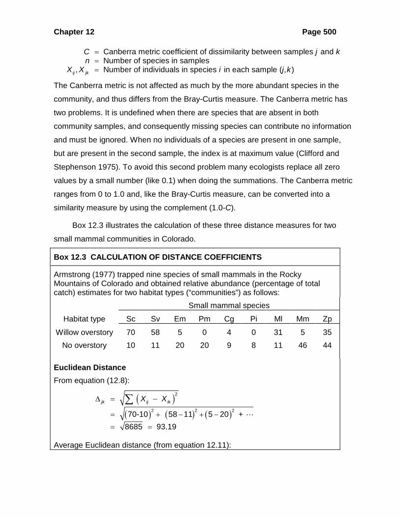
Box 12.3 illustrates the calculation of these three distance measures for two

small mammal communities in Colorado.

Box 12.3 CALCULATION OF DISTANCE COEFFICIENTS

Armstrong (1977) trapped nine species of small mammals in the Rocky Mountains of Colorado and obtained relative abundance (percentage of total catch) estimates for two habitat types (“communities”) as follows:

Small mammal species

Habitat type Sc Sv Em Pm Cg Pi Ml Mm Zp

Willow overstory 70 58 5 0 4 0 31 5 35 No overstory 10

11 20 20 9 8 11 46 44

Euclidean Distance From equation (12.8):

( )( ) ( ) ( )

2

2 2 2

70-10 58 11 5 20 + 8685 93.19

jk ij ikX X∆ = −

= + − + −

= =

∑

Average Euclidean distance (from equation 12.11):

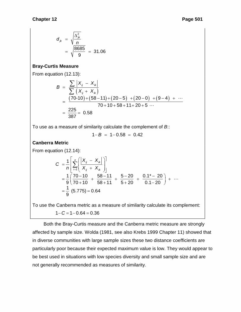
Chapter 12 Page 501

2

8685 31.069

jkjkd

n∆

=

= =

Bray-Curtis Measure From equation (12.13):

( )( ) ( ) ( ) ( ) ( )

70-10 58 11 20 5 20 0 9 4

70 10 58 11 20 5 225 0.58387

ij ik

ij ik

X XB

X X

−=

++ − + − + − + − +

=+ + + + +

= =

∑∑

To use as a measure of similarity calculate the complement of B:: 1 1 0.58 0.42B− = − =

Canberra Metric From equation (12.14):

1

1

1 70 10 58 11 5 20 0.1* 20 9 70 10 58 11 5 20 0.1 201 (5.775) 0.649

nij ik

i ij ik

X XC

n X X=

− =

+ − − − − = + + + + + + + −

= =

∑

To use the Canberra metric as a measure of similarity calculate its complement: 1 1 0.64 0.36C− = − =

Both the Bray-Curtis measure and the Canberra metric measure are strongly

affected by sample size. Wolda (1981, see also Krebs 1999 Chapter 11) showed that

in diverse communities with large sample sizes these two distance coefficients are

particularly poor because their expected maximum value is low. They would appear to

be best used in situations with low species diversity and small sample size and are

not generally recommended as measures of similarity.

Chapter 12 Page 502

12.1.3 Correlation Coefficients

One frequently used approach to the measurement of similarity is to use correlation

coefficients of the standard kind described in every statistics book (e.g. Sokal and

Rohlf 2012, Chap. 15; Zar 2010, Chap. 18). In the terminology used in this chapter,

the Pearson correlation coefficient is given by:

2 2

xyr

x y= ∑∑ ∑

(12.15)

where

2

2 2

2

2 2

Sum of cross products

Sum of squares of

Sum of squares of

, Number of individuals of species in each sample ( , )

ij iki i

ij iki

iji

iji

iki

iki

ij ik

X Xxy X X

n

Xx x X

n

Xy y X

nX X i j k

= = −

= = −

= = −

=

∑ ∑∑ ∑

∑∑ ∑

∑∑ ∑

In order to use the Pearson product-moment correlation coefficient r as a similarity

measure, one must make the usual assumption of a linear relationship between

species abundances in the two communities. If you do not wish to make this

assumption, you can use Spearman's rank correlation coefficient rs or Kendall's tau

instead of r. Both these correlation coefficients range from -1.0 to +1.0.

Correlation coefficients have one desirable and one undesirable attribute.

Romesburg (1984, p. 107) points out that the correlation coefficient is completely

insensitive to additive or proportional differences between community samples. For

example, if sample A is identical to sample B but contains species that are one-half

as abundant as the same species are in sample B, the correlation coefficient gives

the same estimate of similarity, which is a desirable trait. All of the distance measures

we have discussed (except for the adjusted Jaccard and the adjusted Sorensen

indices of Chao et al. 2006) are sensitive to additive and proportional changes in

communities. Table 12.3 illustrates this problem with some hypothetical data.

Chapter 12 Page 503

TABLE 12.3 EFFECTS OF ADDITIVE AND PROPORTIONAL CHANGES IN SPECIES ABUNDANCES ON DISTANCE MEASURES AND CORRELATION COEFFICIENTS. Hypothetical comparison of number of individuals in two communities with four species

Species

1 2 3 4 Community A 50 25 10 5 Community B 40 30 20 10 Community B1 (proportional change 2X) 80 60 40 20 Community B2 (additive change +30) 70 60 50 40 Samples compared

A - B A - B1 A - B2 Average Euclidean distance 7.90 28.50 33.35 Bray-Curtis measure 0.16 0.38 0.42 Canberra metric 0.22 0.46 0.51 Pearson correlation coefficient 0.96 0.96 0.96 Spearman rank correlation coefficient 1.00 1.00 1.00 CONCLUSION: If you wish your measure of similarity to be independent of proportional or additive changes in species abundances, you should not use a distance coefficient to measure similarity.

Correlation coefficients may be undesirable measures of similarity because they

are all strongly affected by sample size, especially in high diversity communities. Field

(1970) recognized this problem and recommended that, when more than half of the

abundances are zero in a community sample, the correlation coefficient should not be

used as a measure of similarity. Wolda (1981) showed the large bias in correlation

coefficients as a measure of similarity because of variations in sample sizes.

12.1.4 Other Similarity Measures

Many other measures of similarity have been proposed. I select here only three to

illustrate the most useful measures of similarity for quantitative data on communities.

Percentage Similarity This measure was proposed by Renkonen (1938) and is

sometimes called the Renkonen index. In order to calculate this measure of similarity,

Chapter 12 Page 504

each community sample must be standardized as percentages, so that the relative

abundances all sum to 100% in each sample. The index is then calculated as:

( )1 2 minimum ,i ii

P p p= ∑ (12.16)

where:

1

2

Percentage similarity between sample 1 and 2 Percentage of species in community sample 1 Percentage of species in community sample 2

i

i

Pp ip i

===

In spite of its simplicity, the percentage similarity measure is one of the better

quantitative similarity coefficient available (Wolda 1981). Percentage similarity is not

affected by proportional differences in abundance between the samples, but is

sensitive to additive changes (c.f. page 502). Box 12.3 illustrates the calculation of

percentage similarity. This index ranges from 0 (no similarity) to 100 (complete

similarity).

Box 12.3 CALCULATION OF PERCENTAGE SIMILARITY, MORISITA, AND HORN INDICES OF SIMILARITY

Nelson (1955) gave the basal areas of the trees in a watershed of western North Carolina for two years before and 17 years after chestnut blight had removed most of the chestnuts: Tree species Basal area (ft2) Percentage composition

1934 1953 1934 1953 Chestnut 53.3 0.9 49.2 1.1 Hickory 18.8 20.7 17.3 25.1 Chestnut oak 10.5 14.2 9.7 17.2 Northern red oak 9.8 5.2 9.0 6.3 Black oak 9.6 17.9 8.9 21.7 Yellow poplar 2.9 13.0 2.7 15.8 Red maple 2.0 3.7 1.8 4.5 Scarlet oak 1.5 6.9 1.4 8.4

Total 108.4 82.5 100.0 100.1 The first step is to express the abundances of the different species as relative abundances (or percentages) which must sum to 100%.

Percentage Similarity

From equation (12.16):

Chapter 12 Page 505

( )1 2PS minimum ,1.1 17.3 9.7 6.3 8.9 2.7 1.8 1.4 49.2%

i ip p== + + + + + + +=

∑

Morisita’s Index of Similarity

From equation (12.17):

( )1 2

2 ij ik

j k

X XC

N Nλ λ λ=

+∑

1(53.3)(52.3) (18.8)(17.8) (10.5)(9.5) (9.8)(8.8)

108.4 (107.4)0.292

λ + + + +=

=

2(0.9)(0) (20.7)(19.7) (14.2)(13.2) 0.167

82.5 (81.5)λ + + +

= =

( )( ) ( )( ) ( )( )( )( )( )

2 53.3 0.9 18.8 20.7 10.5 14.2 1728.96 0.420.292 0.167 108.4 82.5 4104.837

Cλ

+ + + = = =+

From equation (12.20) we can calculate the Morisita-Horn index as:

( ) ( )2 2 2 2

2

/ /ij ik

MHij j ik k j k

X XC

X N X N N N=

+

∑∑ ∑

( ) ( ) ( )( )2 2 2 2

2 2

1728.96 53.3 18.8 0.9 20.7

108.4 82.5108.4 82.51728.96 0.414257.55

MHC = + + + +

+

= =

Horn’s Index of Similarity

From equation (12.21) using the raw data on basal areas and using logs to base 10:

( ) ( ) ( ) ( )( ) ( ) ( ) ( )0

log log log

log log log ij ik ij ik ij ij ik ik

J K J K J J K K

X X X X X X X XR

N N N N N N N N

+ − − = + + − −

∑ ∑ ∑

Breaking down the terms of summation in the numerator:

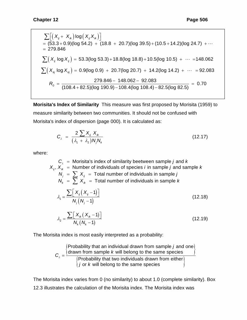
Chapter 12 Page 506

( ) ( )log(53.3 0.9)(log 54.2) (18.8 20.7)(log 39.5) (10.5 14.2)(log 24.7) 279.846

ij ik ij ikX X X X + = + + + + + +=

∑

( )log 53.3(log 53.3) 18.8(log 18.8) 10.5(log 10.5) 148.062ij ijX X = + + + =∑

( )log 0.9(log 0.9) 20.7(log 20.7) 14.2(log 14.2) 92.083kj kjX X = + + + =∑

0279.846 148.062 92.083 0.70

(108.4 82.5)(log 190.9) 108.4(log 108.4) 82.5(log 82.5)R − −

= =+ − −

Morisita's Index of Similarity This measure was first proposed by Morisita (1959) to

measure similarity between two communities. It should not be confused with

Morisita's index of dispersion (page 000). It is calculated as:

( )1 2

2 ij ik

j k

X XC

N Nλ λ λ=

+∑ (12.17)

where:

Morisita's index of similarity beetween sample and , Number of individuals of species in sample and sample

Total number of individuals in sample Total n

ij ik

j ij

k ik

C j kX X i j k

N X jN X

λ === == =∑

umber of individuals in sample k∑

( )( )1

1

1ij ij

j j

X X

N Nλ

− =−

∑ (12.18)

( )( )2

11

ik ik

k k

X XN N

λ − =

−∑ (12.19)

The Morisita index is most easily interpreted as a probability:

{ }{ }

Probability that an individual drawn from sample and onedrawn from sample will belong to the same species

Probability that two individuals drawn from either or will belong to the same species

jk

C

j kλ =

The Morisita index varies from 0 (no similarity) to about 1.0 (complete similarity). Box

12.3 illustrates the calculation of the Morisita index. The Morisita index was

Chapter 12 Page 507

formulated for counts of individuals and not for other abundance estimates based on

biomass, productivity, or cover. Horn (1966) proposed a simplified Morisita index (=

Morisita-Horn index) in which all the (-1) terms in equations (12.17) and (12.18) are

ignored:

( ) ( )2 2 2 2

2

/ /ij ik

MHij j ik k j k

X XC

X N X N N N=

+

∑∑ ∑

(12.20)

where = Morisita-Horn index of similarity (Horn, 1966)MHC

and all other terms are as defined above. This formula is appropriate when the

original data are expressed as proportions rather than numbers of individuals and

should be used when the original data are not numbers but biomass, cover, or

productivity (see page 000).

The Morisita index of similarity is nearly independent of sample size, except for

samples of very small size. Morisita (1959) did extensive simulation experiments to

show this, and these results were confirmed by Wolda (1981), who recommended

Morisita's index as the best overall measure of similarity for ecological use.

Horn’s Index of Similarity Horn (1966) developed another index of similarity based

on information theory. It can be calculated directly from raw data (numbers) or from

relative abundances (proportions or percentages).

( ) ( ) ( ) ( )( ) ( ) ( ) ( )0

log - log - log =

+ log + - log - log ij ik ij ik ij ij ik ik

J K J K J J K K

X X X X X X X XR

N N N N N N N N

+

∑ ∑ ∑ (12.21)

where:

0 Horn's index of similarity for samples and , Number of individuals of species in sample and sample

Total number of individuals in sample Total number of

ij ik

J ij

K ik

R j kX X i j k

N X jN X

=== == =∑∑ individuals in sample k

and all summations are over all the n species. Horn's index can be calculated from

this equation using numbers or using proportions to estimate relative abundances.

Note that the value obtained for the Horn’s index is the same whether numbers or

Chapter 12 Page 508

proportions are used in equation (12.21) and is not affected by the base of logarithms

used.

The Horn’s index is relatively little affected by sample size (Figure 12.4),

although it is not as robust as Morisita's index. Box 12.3 illustrates the calculation of

Horn’s index.

Higher diversity(750 species)

Lower diversity(150 species)

Size of smaller sample100 200 500 1000 5000

Sim

ilarit

y Co

effic

ient

0.0

0.2

0.4

0.6

0.8

1.0

Size of smaller sample100 200 500 1000 5000

0.0

0.2

0.4

0.6

0.8

1.05000 5000

10001000

Horn'sindex(R0)

500

500200

200

Figure 12.4 Expected maximum values of Horn’s index of similarity. The number of individuals in the smaller of the two community samples is given on the X axis, and the lines connect samples of equal size for larger community sample (n = 5000, 1000, 500, 200; a different symbol is used for each of these sample sizes). A highly diverse community is shown on the left and a lower-diversity community on the right. Horn’s measure is relatively little affected by sample size and is recommended as possible alternatives to Morisita’s index. (From Wolda, 1981).

12.2 WHICH SIMILARITY MEASURES ARE TO BE PREFERRED?

With so many proposed measures of community similarity, the novice ecologist is

easily perplexed about what to use for his or her data. I attempt here to state what

appears to be a consensus among quantitative statisticians about these indices.

With only presence-absence data the options are very limited, and either the

Jaccard or the Sorensen indices seem the best choice. But when samples sizes are

not large enough to capture all the species present, it is now well known that all these

presence-absence indices are biased too low, and the bias is likely to be substantial

for communities with high species numbers and many rare species (Chao et al. 2006,

Magurran 2004). Equal sampling effort in the two communities does not remove this

Chapter 12 Page 509

bias. It is theoretically possible that the Jaccard and Sorensen indices could be

upwardly biased but this seems to be most unusual.

There are more choices among the abundance based similarity measures. Chao

et al. (2006) carried out an extensive set of simulations on a set of rain forest tree

data from Costa Rica. They sampled 5000 times at random from the data set of 86

species given in her paper and estimated the average bias for a range of sampling

intensities. Table 12.4 gives these results for 6 of the measures of similarity.

Table 12.4 PERCENTAGE RELATIVE BIAS FROM SAMPLING OF A RAINFOREST SET OF QUADRAT DATA ON SEEDLINGS VERSUS LARGE TREES IN COSTA RICA. Individual trees in the original raw data were sampled with replacement at the specified sampling intensities, and the similarity indices calculated. The simulation was repeated 5000 times to obtain these averages.

Sampling fraction Index True

value 10% vs

10% 10% vs.

60% 50% vs

50% 40% vs

90% 90% vs

90%

Presence-absence based

Jaccard 0.30 -64a -43 -32 -23 -19

Sorensen 0.46 -58 -37 -27 -18 -15

Abundance based

Bray-Curtis 0.24 -35 38 -14 45 -9

Morisita-Horn 0.74 -38 -15 -10 -7 -5

Adjusted Jaccard 0.40 -30 -5 4 2 3

Adjusted Sorensen 0.58 -26 -5 2 1 2 a Negative values indicate an underestimate of the true value, positive values an overestimate of the true value

Table 12.4 shows that at very low rates of sampling, all the estimators perform poorly.

The presence-absence estimators of similarity always underestimate true similarity,

as shown by Wolda (1981). The Bray-Curtis measure performs very poorly and

should be used only when the sampling fractions are equal (Chao et al. 2006). The

Morisita-Horn index (eq. 12.18) performs well, but for these simulations the adjusted

Jaccard and the adjusted Sorensen indices (from Table 12.2) performed best of all

the abundance-based similarity measures.

Chapter 12 Page 510

Obtaining confidence limits for all these estimators must be done with bootstrap

techniques (see Chapter 16). Both of the computer programs devoted to biodiversity

measurements can provide standard errors for each index. The program SPADE from

Anne Chao (http://chao.stat.nthu.edu.tw/softwarece.html) and the program EstimateS

from Robert Colwell (http://viceroy.eeb.uconn.edu/estimates/index.html) calculate

these standard errors from bootstrapped samples.

12.2 DATA STANDARDIZATION

Data to be used for community comparisons may be provided in several forms, and

we have already seen examples of data as numbers and proportions (or percentages)

(Table 12.1). Here we discuss briefly some rules of thumb that are useful in deciding

how data should be standardized and when. Romesburg (1984, Chap. 8) and Clifford

and Stephenson (1975, Chap. 7) have discussed this problem in more detail.

A considerable amount of judgment is involved in deciding how data should be

summarized before similarity values are calculated. Three broad strategies exist:

apply transformations, use standardization, and do nothing. No one strategy can be

universally recommended and much depends upon your research objectives.

Transformations1 may be applied to the numbers of individuals counted in each

species. Typical transformations are to replace each of the original counts (X) with

X or 1X + , or in extreme cases by log (X+1.0). These transformations will reduce

the importance of extreme values, for example if one species is extremely abundant

in one sample. In general, transformations are also used to reduce the contributions

of the common species and to enhance the contributions of the rare species.

Transformations also affect how much weight is given to habitat patchiness. If a

single patch contains one highly abundant species, fox example, this one patch may

produce a strong effect on the calculated similarity values. A transformation can help

to smooth out these variations among patches, if you wish to do this smoothing on

ecological grounds. If a transformation is used, it is applied before the similarity index

is calculated.

Chapter 12 Page 511

Standardization of data values can be done in several ways. The most familiar

standardization is to convert absolute numbers to proportions (Table 12.1). Note that

in doing this all differences in population sizes between sites are lost from the data.

Whether or not you wish to omit such differences from your analysis will determine

your use of standardization. Romesburg (1984, Chap. 7) discusses other types of

standardization.

The two most critical questions you must answer before you can decide on the

form your data should take are:

1. Are a few species excessively common or rare in your samples such that these extreme values distort the overall picture? If yes, use a transformation. You will have to use ecological intuition to decide what "excessively" means. A ten-fold difference in abundance between the most common and the next most common species might be a rule of thumb for defining "excessively common".

2. Do you wish to include the absolute level of abundance as a part of the measurement of similarity between communities? If no, use standardization to proportions to express relative abundances. If you do not use either of these strategies, you should remember that if you do nothing to your raw data, you are still making a decision about what components of similarity to emphasize in your analysis.

One additional question about data standardization is when data may be deleted

from the analysis. Many ecologists routinely eliminate rare species from their data

before they apply a similarity measure. This practice is rooted in the general

ecological feeling that species represented by only 1 or 2 individuals in a large

community sample cannot be an important and significant component of the

community (Clifford and Stephenson 1975, p. 86). It is important that we try to use

only ecological arguments about eliminating species from data sets, and we try to

eliminate as few species as possible (Stephenson et al. 1972).

The most important point to remember is that data transformation changes the

values of almost all of the coefficients of similarity. It is useful to decide before you

begin your analysis on what type of data standardization is appropriate for the

questions you are trying to answer. You must do this standardization for a priori

1 See Chapter 16 (page 000) for more discussion of transformations.

Chapter 12 Page 512

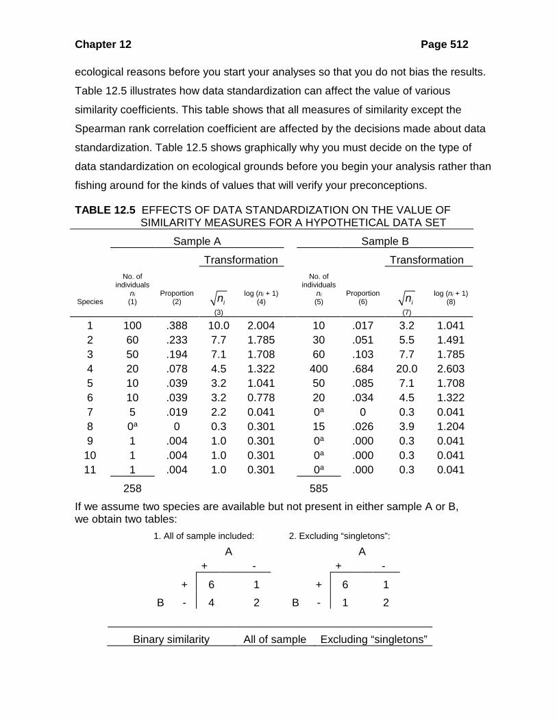
ecological reasons before you start your analyses so that you do not bias the results.

Table 12.5 illustrates how data standardization can affect the value of various

similarity coefficients. This table shows that all measures of similarity except the

Spearman rank correlation coefficient are affected by the decisions made about data

standardization. Table 12.5 shows graphically why you must decide on the type of

data standardization on ecological grounds before you begin your analysis rather than

fishing around for the kinds of values that will verify your preconceptions.

TABLE 12.5 EFFECTS OF DATA STANDARDIZATION ON THE VALUE OF SIMILARITY MEASURES FOR A HYPOTHETICAL DATA SET

Sample A Sample B

Transformation Transformation

Species

No. of individuals

ni (1)

Proportion (2)

in

(3)

log (ni + 1) (4)

No. of individuals

ni (5)

Proportion (6)

in

(7)

log (ni + 1) (8)

1 100 .388 10.0 2.004 10 .017 3.2 1.041 2 60 .233 7.7 1.785 30 .051 5.5 1.491 3 50 .194 7.1 1.708 60 .103 7.7 1.785 4 20 .078 4.5 1.322 400 .684 20.0 2.603 5 10 .039 3.2 1.041 50 .085 7.1 1.708 6 10 .039 3.2 0.778 20 .034 4.5 1.322 7 5 .019 2.2 0.041 0a 0 0.3 0.041 8 0a 0 0.3 0.301 15 .026 3.9 1.204 9 1 .004 1.0 0.301 0a .000 0.3 0.041

10 1 .004 1.0 0.301 0a .000 0.3 0.041 11 1 .004 1.0 0.301 0a .000 0.3 0.041

258 585 If we assume two species are available but not present in either sample A or B, we obtain two tables: 1. All of sample included: 2. Excluding “singletons”: A A + - + -

+ 6 1 + 6 1 B - 4 2 B - 1 2

Binary similarity All of sample Excluding “singletons”

Chapter 12 Page 513

coefficients included (species 9, 10, 11)

Jaccard 0.54 0.75 Sorensen 0.71 0.86 Simple matching 0.61 0.80 Baroni-Urbani and Buser 0.65 0.83 For the quantitative measures of similarity and dissimilarity: Type of data standardization

Coefficient

Raw data (1), (5)

Proportions (2), (6) in

(3), (7)

log (ni + 1) (4), (8)

Euclidean distance 118.88 0.22 5.48 0.70 1 - Bray-Curtis 0.31 0.32 0.59 0.71 1 - Canberra metric 0.26 0.26 0.50 0.51 Pearson correlation 0.02 0.02 0.32 0.60 Spearman correlation 0.60 0.60 0.60 0.60 Percentage similarity -- 32 58b 72b Morisita’s index 0.26 0.26 0.65 0.85 Horn index 0.56 0.56 0.81 0.85 a Zero values replaced by 0.1 for calculations of transformations. b Percentages calculated on the transformed values instead of the raw data.

12.3 CLUSTER ANALYSIS

The measurement of similarity between samples from communities may be useful as

an end in itself, especially when there are very few samples or only a few

communities. In other cases we have many samples to analyze and we now discuss

techniques for grouping samples which are similar to one another.

Clustering methods are methods of achieving a classification of a series of

samples. Classification may not be a desirable end goal for all ecological problems,

and we may wish to treat variation as continuous instead of trying to classify samples

into a series of groups. We will continue on the assumption that this methodological

decision to classify has been made. There are four major questions we must answer

before we can decide on a method of classification (Pielou 1969). The method of

classification can be:

Chapter 12 Page 514

1. Hierarchical or reticulate: hierarchical classifications are like a tree, reticulate classifications overlap like a net; ordinary taxonomic classifications are hierarchical; everyone uses hierarchical classifications because they are easier to understand. 2. Divisive or agglomerative: in a divisive classification we begin with the whole set of samples and divide it up into classes; in agglomerative classification we start at the bottom and work upward, beginning with the individual samples. Divisive techniques ought to be more accurate because chance anomalies with individual samples may start agglomerative techniques off with some bad combinations which snowball as more agglomeration proceeds. 3. Monothetic or polythetic: in a monothetic classification two sister groups are distinguished by a single attribute, such as the presence of one species. In a polythetic classification over-all similarity is used, based on all the attributes (species). Monothetic classifications are simple to understand and easy to determine but can waste information and may be poor if we choose the wrong attribute. 4. Qualitative or quantitative data: the main argument for using quantitative data is to avoid weighing the rare species as much as the common ones. This is a question of ecological judgment for each particular situation. In some cases only qualitative (binary) data are available.

The most important point to note at this stage is that there is no one single kind

of classification, no "best" system of grouping samples. We must rely on our

ecological knowledge to evaluate the end results of any classification.

Cluster analysis is the general term applied to the many techniques used to

build classifications. Many of these are reviewed by Romesburg (1984), Hair et al.

2010, and by Everitt et al. 2011). I will discuss here only a couple of simpler

techniques, all of which are hierarchical, agglomerative, polythetic techniques.

Virtually all of the techniques of cluster analysis demand a great deal of calculation

and hence have become useful only with the advent of computers.

12.3.1 Single Linkage Clustering

This technique is the simplest form of hierarchical, agglomerative cluster analysis. It

has been called the nearest neighbor method. We will use the data in Table 12.5 to

illustrate the calculations involved in cluster analysis.

Begin (as in all cluster analysis of an agglomerative type) with a matrix of

similarity (or dissimilarity) coefficients. Table 12.7 gives the similarity matrix for the

seabird data in Table 12.6, with the complement of the Canberra metric being used

as the similarity measure.

Chapter 12 Page 515

Given this matrix in Table 12.7, the rules for single linkage clustering are as

follows:

1. To start, find the most similar pair(s) of samples - this is defined to be the first cluster.

2. Next, find the second most similar pair(s) of samples OR highest similarity between a sample and the first cluster, whichever is greater.

Definitions: For single linkage clustering -

{ } { }{ }

Similarity between a sample Similarity between the sample and the and an existing cluster member of that clusterSimilarity between two Similarity between the two existing clusters

nearestnear

=

= { }members of the clustersest

3. Repeat the cycle specified in (2) until all the samples are in one big cluster. Box 12.4 illustrates the application of these rules to the data in Table 12.6. The

advantage of single linkage clustering is that it is simple to calculate. Its major

disadvantage is that one inaccurate sample may compromise the entire clustering

process.

Chapter 12 Page 516

TABLE 12.6 RELATIVE ABUNDANCES (PROPORTIONS) OF 23 SPECIES OF SEABIRDS ON 9 COLONIES IN NORTHERN POLAR AND SUBPOLAR AREASa

Cape Hay, Bylot Island

Prince Leopold Island, eastern Canada

Coburg Island, eastern Canada

Norton Sound, Bering Sea

Cape Lisburne,Chukchi Sea

Cape Thompson, Chukchi Sea

Skomer Island, Irish Sea

St. Paul Island, Bering Sea

St. George Island, Bering Sea

Northern fulmar 0 .3422 0 0 0 0 .0007 .0028 .0278

Glaucous-winged gull .0005 .0011 .0004 .0051 .0004 .0007 0 0 0

Black-legged kittiwake .1249 .1600 .1577 .1402 .1972 .0634 .0151 .1221 .0286

Red-legged kittiwake 0 0 0 0 0 0 0 .0087 .0873

Thick-billed murre .8740 .4746 .8413 .0074 .2367 .5592 0 .4334 .5955

Common murre 0 0 0 .7765 .5522 .3728 .0160 .1537 .0754

Black guillemot .0006 .02200. .0005 0 .0013 .00001 0 0 0

Pigeon guillemot 0 0 0 0 0 .00003 0 0 0

Horned puffin 0 0 0 .0592 .0114 .0036 0 .0173 .0111

Tufted puffin 0 0 0 .0008 .0002 0 0 .0039 .0024

Atlantic puffin 0 0 0 0 0 0 .0482 0 0

Pelagic cormorant 0 0 0 .0096 .0006 .0001 .0001 0 0

Red-faced cormorant 0 0 0 0 0 0 0 .0099 .0020

Shag 0 0 0 0 0 0 .0001 0 0

Parakeet auklet 0 0 0 .0012 0 0 0 .1340 .0595

Crested auklet 0 0 0 0 0 0 0 .0236 .0111

Least auklet 0 0 0 0 0 0 0 .0906 .0992

Razorbill 0 0 0 0 0 0 .0130 0 0

Manx shearwater 0 0 0 0 0 0 .7838 0 0

Storm petrel 0 0 0 0 0 0 .0389 0 0

Chapter 12 Page 517

Herring gull 0 0 0 0 0 0 .0229 0 0

Great black-backed gull 0 0 0 0 0 0 .0001 0 0

Lesser black backed gull 0 0 0 0 0 0 .0603 0 0 a Data from Hunt et al. (1986).

Chapter 12 Page 518

TABLE 12.7 MATRIX OF SIMILARITY COEFFICIENTS FOR THE SEABIRD DATA IN TABLE 12.6. ISLANDS ARE PRESENTED IN SAME ORDER AS IN TABLE 12.6a

CH PLI CI NS CL CT SI SPI SGI

CH 1.0 0.88 0.99 0.66 0.77 0.75 0.36 0.51 0.49 PLI 1.0 0.88 0.62 0.70 0.71 0.36 0.51 0.49 CI 1.0 0.66 0.78 0.75 0.36 0.50 0.48 NS 1.0 0.73 0.64 0.28 0.53 0.50 CL 1.0 0.76 0.29 0.51 0.49 CT 1.0 0.34 0.46 0.45 SI 1.0 0.19 0.20 SPI 1.0 0.80 SGI 1.0 a The complement of the Canberra metric (1.0 - C) is used as the index of similarity. Note that the matrix is symmetrical about the diagonal.

Box 12.4 SINGLE LINKAGE CLUSTERING OF THE DATA IN TABLES 12.6 AND 12.7 ON SEABIRD COMMUNITIES

1. From these tables we can see that the most similar pair of communities is Cape Hay and Coburg Island, and they join to form cluster 1 at similarity 0.99. 2. The next most similar community is Prince Leopold Island, which is similar to Cape Hay and Coburg Island. From the definition:

{ } Similarity between the sampleSimilarity between a sample and the member ofand an existing cluster the clusternearest

=

this occurs at similarity 0.88, and we have now a single cluster containing three communities: Prince Leopold Island, Cape Hay, and Coburg Island. 3. The next most similar pair is St. Paul and St. George Islands, and they join to form a second cluster at similarity 0.80. 4. The next most similar community is Cape Lisburne, which joins the first cluster at similarity 0.78 (the similarity between Cape Lisburne and Coburg Island). The first cluster now has four islands in it. 5. The next most similar community is Cape Thompson, which joins this large cluster at similarity 0.76 because this is the Cape Thompson-Cape Lisburne similarity. This cluster now has five communities in it.

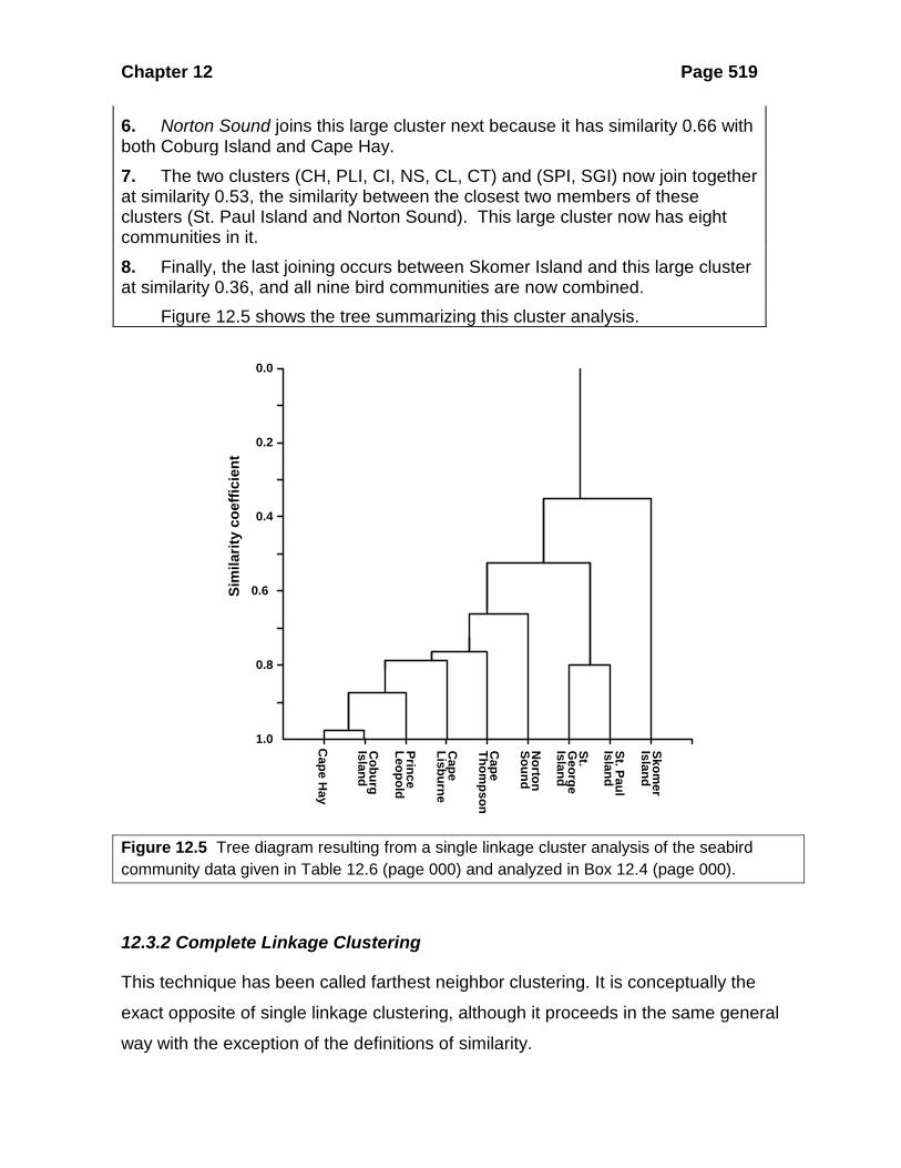
Chapter 12 Page 519

6. Norton Sound joins this large cluster next because it has similarity 0.66 with both Coburg Island and Cape Hay. 7. The two clusters (CH, PLI, CI, NS, CL, CT) and (SPI, SGI) now join together at similarity 0.53, the similarity between the closest two members of these clusters (St. Paul Island and Norton Sound). This large cluster now has eight communities in it. 8. Finally, the last joining occurs between Skomer Island and this large cluster at similarity 0.36, and all nine bird communities are now combined. Figure 12.5 shows the tree summarizing this cluster analysis.

1.0

0.8

0.6

0.4

0.2

0.0

Cape H

ay

Coburg

Island

PrinceLeopold

Cape

Lisburne

Cape

Thompson

Norton

Sound

St. G

eorgeIsland

St. PaulIsland

Skomer

IslandSi

mila

rity

coef

ficie

nt

Figure 12.5 Tree diagram resulting from a single linkage cluster analysis of the seabird community data given in Table 12.6 (page 000) and analyzed in Box 12.4 (page 000).

12.3.2 Complete Linkage Clustering

This technique has been called farthest neighbor clustering. It is conceptually the

exact opposite of single linkage clustering, although it proceeds in the same general

way with the exception of the definitions of similarity.

Chapter 12 Page 520

Definitions For complete linkage clustering:

{ } { }{ }

Similarity between a sample Similarity between the sample and the and an existing cluster member of that clusterSimilarity between two Similarity between the two existing clusters

farthest=

= { }members of the clustersfarthest

One of the possible difficulties of single linkage clustering is that it tends to produce

long, strung-out clusters. This technique often tends to the opposite extreme,

producing very tight compact clusters. Like single linkage clustering, complete linkage

clustering is very easy to compute.

Because neither of these two extremes is usually desirable, most researchers

using cluster analysis have suggested modifications of single and complete linkage

clustering to produce intermediate results.

12.3.3 Average Linkage Clustering

These techniques were developed to avoid the extremes introduced by single linkage

and complete linkage clustering. All types of average linkage clustering require

additional computation at each step in the clustering process, and hence are normally

done with a computer (Romesburg, 1984). In order to compute the average similarity

between a sample and an existing cluster, we must define more precisely the types of

"averages" to be used.

The most frequently used clustering strategy is called by the impressive name

unweighted pair-group method using arithmetic averages, abbreviated UPGMA

(Romesburg 1984). This clustering strategy proceeds exactly as before with the single

exception of the definition:

Definitions For arithmetic average clustering by the unweighted pair-group method:

{ } Arithmetic mean of similaritiesSimilarity between a sample between the sample and alland an existing cluster the members of the cluster

=

( )( )1 J K JK

J K

S St t

= ∑ (12.22)

Chapter 12 Page 521

where:

( )( )

( ) Similarity between clusters and Number of samples in cluster 1 Number of samples in cluster 2

J K

J

K

S J Kt Jt K

== ≥= ≥

The same formula applies to dissimilarity coefficients, such as Euclidian distances.

Box 12.5 illustrates the calculations for average linkage clustering by the

UPGMA method. Normally one would not do all these tedious calculations but would

let the computer do the analysis. There are many different clustering programs

available for computers.

There are several additional methods of cluster analysis available, and I have

only scratched the surface of a complex technique in this chapter. It is encouraging

that Romesburg (1984) after a detailed analysis of various methods of clustering

comes out recommending the UPGMA method for most types of cluster applications.

Cluster analysis should be used to increase our ecological insight and not to baffle

the reader, and for this reason simpler methods are often preferable to very complex

ones.

Box 12.5 AVERAGE LINKAGE CLUSTERING OF THE DATA IN TABLES 12.6 AND 12.7 USING THE UNWEIGHTED PAIR-GROUP METHOD (UPGMA)

1. From the data in Table 12.6 the most similar pair of communities is Cape Hay and Coburg Island, and they join at similarity 0.99 to make cluster 1. 2. We now recompute the entire similarity matrix for the seven remaining communities and cluster 1, using the definition in equation (12.19):

( )( )1

J K JKJ K

S St t

= ∑

where:

( ) Similarity between clusters and Number of samples in cluster Number of samples in cluster Observed similarity coefficients between each of the samples in and

J K

J

K

JK

S J Kt Jt K

SJ K

====

For example, the similarity between cluster J (Cape Hay + Coburg Island) and cluster K (St. George Island) is given by:

Chapter 12 Page 522

( ) ( ) ( )( )1 1 0.49 0.48 0.485

2 1J K JKJ K

S St t

= = + =∑

The largest similarity value in this recomputed matrix is that between Prince Leopold Island and cluster 1:

( )( ) ( )( )1 0.88 0.88

1 2 0.88

J KS = +

=

3. We recompute the entire similarity matrix for the seven groups. The next largest similarity coefficient is that between St. Paul Island and St. George Island at similarity 0.80, forming cluster 2. We now have two clusters and four remaining individual community samples. 4. We recompute the similarity matrix for the six groups, and the next largest similarity coefficient is for Cape Lisburne and Cape Thompson, which join at similarity 0.76, forming cluster 3. We now have three clusters and two remaining individual community samples. 5. We again recompute the similarity matrix for the five groups, and the next largest similarity coefficient is for cluster 3 (CL, CT) and cluster 1 (CH, CI, and PLI):

( )( ) ( )( )1 0.77 0.78 0.70 0.75 0.75 0.71

2 3 0.74

J KS = + + + + +

=

so cluster 1 now has five members formed at similarity 0.74. 6. We again recompute the similarity matrix for the four groups, and the largest similarity coefficient is for Norton Sound and cluster 1 (CH, CI, PLI, CL, CT):

( )( ) ( )( )1 0.66 0.62 0.66 0.73 0.64

1 5 0.66

J KS = + + + +

=

so cluster 1 now has six members. 7. We recompute the similarity matrix for the three groups from equation (12.19) and obtain: Cluster 1 Skomer Island Cluster 2

Cluster 1 1.0 0.33 0.49 Skomer Island -- 1.0 0.19 Cluster 2 -- -- 1.0 For example, the similarity between cluster 1 and cluster 2 is

Chapter 12 Page 523

( )( )( )1 (0.51 0.51 0.50 0.53 0.51 0.46 0.49

6 2 0.49 0.48 0.50 0.49 0.45)

0.493

J KS = + + + + + +

+ + + + +=

Thus, clusters 1 and 2 are joined at similarity 0.49. We now have two groups --

Skomer Island and all the rest in one big cluster.

8. The last step is to compute the average similarity between the remaining two groups:

( )( ) ( )( )1 0.36 0.36 0.36 0.28 0.29 0.34 0.19 0.20

1 8 0.297

J KS = + + + + + + +

=

so the final clustering is at similarity 0.3. The clustering tree for this cluster analysis is shown in Figure 12.6. It is very similar to that shown in Figure 12.5 for single linkage clustering.

1.0

0.8

0.6

0.4

0.2

0.0

Cape H

ay

Coburg

Island

PrinceLeopold

Cape

Lisburne

Cape

Thompson

Norton

Sound

St. G

eorgeIsland

St. PaulIsland

Skomer

IslandSi

mila

rity

coef

ficie

nt

Figure 12.6 Tree diagram resulting from average linkage clustering using the unweighted pair-group method (UPGMA) on the seabird community data given in Table 12.6 (page 000)and analyzed in Box 12.5 (page 000).

Chapter 12 Page 524

12.4 RECOMMENDATIONS FOR CLASSIFICATIONS

You should begin your search for a classification with a clear statement of your

research goals. If a classification is very important as a step to achieving these goals,

you should certainly read a more comprehensive book on cluster analysis, such as

Romesburg (1984), or .Everitt et al. (2011).

You must first decide on the type of similarity measure you wish to use.

Measures of similarity based on binary data are adequate for some classification

purposes but are much weaker than quantitative measures. Of all the similarity

measures available the Morisita-Horn index of similarity is clearly to be preferred

because it is not dependent on sample size (Wolda 1981). Most ecologists seem to

believe that the choice of a similarity measure is not a critical decision but this is

definitely not the case, particularly when one realizes that a joint decision about data

standardization or transformation and the index to be used can greatly affect the

resulting cluster analysis. If data are transformed with a log transformation, Wolda

(1981) suggests using the Morisita-Horn index (equation 12.20) or the Percentage

Similarity index (equation 12.16)

In addition to all these decisions, the choice of a clustering algorithm can also

affect the resulting tree. Romesburg (1984, p. 110-114) discusses an interesting

taxonomic cluster analysis using bone measurements from several species of

hominoids. Each similarity coefficient produced a different taxonomic tree, and the

problem of which one is closer to the true phylogenetic tree is not immediately clear

without independent data. The critical point is that, given a set of data, there is no one

objective, "correct", cluster analysis. If you are to evaluate these different cluster

analyses, it must be done with additional data, or ecological insight.

This is and must remain the central paradox of clustering methods - that each

method is exact and objective once the subjective decisions have been made about

the similarity index and data standardization.

Finally, virtually none of the similarity measures has a statistical probability

distribution and hence you cannot readily set confidence intervals on these estimates

Chapter 12 Page 525

of similarity. It is therefore not possible to assess probable error without taking

replicate community samples. There is no general theory to guide you in the sample

size you require from each community. Wolda (1981) suggests that more than 100

individuals are always needed before it is useful to calculate a similarity index (unless

the species diversity of the community is very low). A reasonable community sample

would probably be 200-500 individuals for low diversity communities, and 10 times the

number of species for high diversity communities. These are only rule-of-thumb

guesses and a rigorous statistical analysis of sampling for similarity is waiting to be

done.

12.5 OTHER MULTIVARIATE TECHNIQUES

Classification by means of cluster analysis is by no means the only way to analyze

community data. Plant ecologists have developed a series of multivariate techniques

that are useful for searching for patterns in community data. These methods have

grown in complexity so that they are now best treated in a separate book. Legendre

and Legendre (2012) have provided an excellent overview of these methods for

ecologists, and students are referred to their book. Gradient analysis, ordination, and

cluster analysis are important methods for community ecologists and require detailed

understanding before being used.

12.6 SUMMARY

Communities may be more or less similar and ecologists often wish to express this

similarity quantitatively and to classify communities on the basis of this similarity.

Similarity measures may be binary, based on presence/absence data, or quantitative

based on some measure of importance like populations size, biomass, cover, or

productivity. There are more than two dozen similarity measures and I describe 4

binary coefficients and 8 quantitative measures that are commonly used. Some

measures emphasize the common species in the community, others emphasize the

rare species. Many of the commonly used measures of similarity are strongly

dependent on sample size, and should be avoided if possible. The Morisita-Horn

index and the Adjusted Jaccard and Adjusted Sorensen indices of similarity are

Chapter 12 Page 526

recommended for quantitative data because they are not greatly affected by sample

size. For all measures of similarity, large samples (>10 shared species between the

samples) are recommended.

Cluster analysis is a method for generating classifications from a series of

community samples. Many different types of cluster analysis have been developed,

and there is no one "correct" or ideal system. Most ecological data can be classified

simply by average linkage clustering (UPGMA) and this technique is recommended

for general usage.

Data to be input into cluster analysis may be as raw numbers, transformed by

square root or logarithmic transformations, or expressed as proportions (relative

abundance). Decisions about the type of data to be used, the similarity index, and the

clustering algorithm should be made before any analysis is done on the basis of the

research objectives you wish to achieve. Cluster analysis and the measurement of

ecological similarity are two parts art and one part science, and ecological intuition is

essential to success.

SELECTED REFERENCES

Chao, A., Chazdon, R.L., Colwell, R.K., and Shen, T.-J. 2006. Abundance-based similarity indices and their estimation when there are unseen species in samples. Biometrics 62(2): 361-371.

Everitt, B.S., Landau, S., Leese, M., and Stahl, D. 2011. Cluster Analysis. 5th ed. Wiley, New York.

Huhta, V. 1979. Evaluation of different similarity indices as measures of succession in arthropod communities of the forest floor after clear-cutting. Oecologia 41: 11-23.

Jackson, D.A., K.M. Somers, and H.H. Harvey. 1989. Similarity coefficients: measures of co-occurrence and association or simply measures of occurrence? American Naturalist 133: 436-453.

Legendre, L. and P. Legendre. 2012. Numerical Ecology. 3rd ed. Elsevier, Amsterdam.

Morisita, M. 1959. Measuring of interspecific association and similarity between communities. Memoirs of the Faculty of Science, Kyushu University, Series E (Biology) 3: 65-80.

Chapter 12 Page 527

Romesburg, H.C. 1984. Cluster Analysis For Researchers. Lifetime Learning Publications, Belmont, California.

Wolda, H. 1981. Similarity indices, sample size and diversity. Oecologia 50: 296-302.

QUESTIONS AND PROBLEMS

12.1 A Christmas bird count in three areas of Manitoba in 1985 produced the following data:

No. of individuals counted

Brandon Delta Marsh Winnipeg Canada goose 0 0 2 Mallard 0 0 5 Northern goshawk 0 1 2 Golden eagle 0 1 0 American kestrel 0 0 3 Merlin 2 0 1 Gray partridge 29 45 112 Ruffed grouse 4 0 0 Sharp-tailed grouse 48 11 1 Rock dove 907 8 6,179 Mourning dove 0 0 2 Great horned owl 6 1 5 Snowy owl 3 1 2 Barred owl 0 0 1 Black-backed woodpecker 0 a 0 Downy woodpecker 12 4 79 Hairy woodpecker 13 8 51 Horned lark 0 1 0 Bluejay 29 18 99 Black-billed magpie 89 28 31 American crow 0 3 2 Common raven 2 1 0 Blackcapped chickadee 134 26 595 Red breasted nuthatch 3 0 7 White breasted nuthatch 36 11 169 Brown creeper 0 0 1 Golden crowned kinglet 2 0 0 American robin 4 0 2 Varied thrush 1 0 0

Chapter 12 Page 528

Bohemian waxwing 30 45 192 Cedar waxwing 35 0 0 Northern shrike 2 4 3 European starling 55 52 982 White throated sparrow 0 0 1 Dark eyed junco 4 5 11 Lapland longspur 0 3 63 Snow bunting 2 4,019 68 Red-winged blackbird 0 1 2 Rusty blackbird 0 0 5 Brewer’s blackbird 0 7 0 Common grackle a 0 1 Pine grosbeak 150 48 701 Purple finch a 0 2 Red crossbill 0 a 0 White-winged crossbill 1 0 0 Common redpoll 499 1,191 859 Hoary redpoll 5 35 16 Pine siskin 0 2 14 American goldfinch 0 2 3 Evening grosbeak 136 46 30 House sparrow 3,024 855 11,243

Total individuals 5,267 6,483 21,547 Total species 30 31 40 Total species in Manitoba = 61

a Species known to be in the area but not seen on the day of the count.

The amount of effort expended in these counts can not be assumed to be equal in the three areas.

(a) Choose a binary coefficient that you think should be used for data of this type and calculate the similarity between these three winter bird communities. (b) Discuss what type of data standardization might be done before a quantitative similarity index is calculated. (c) Calculate the value of the most appropriate quantitative index of similarity for these three bird communities

12.2 Calculate the Adjusted Sorensen index for the data in Table 12.1, page 000, and also the Morisita-Horn index. Why do these two measures differ in value?

Chapter 12 Page 529

12.3 Compare and contrast the evaluations of similarity indices by Huhta (1979) and Wolda (1981).

12.4 Recalculate the similarity matrix in Table 12.6 using the Morisita-Horn index (eq. 12.20) and use these data to prepare an average linkage cluster analysis similar to that in Box 12.5. How do your results differ from those reported in Figure 12.6?

12.5 The species composition of the groundfish community off Nova Scotia was measured by Mahon et. al. (1984), who obtained these data for two parts of the Bay of Fundy:

Species Average no. of individuals per tow

Percent

West Fundy area Redfish 12.7 14.1 White hake 11.3 12.6 Haddock 10.1 11.3 Cod 9.8 10.9 Spiny dogfish 9.3 10.4 Thorny skate 5.8 6.5 Plaice 4.9 5.5 Witch 4.5 5.0 Longhorn sculpin 4.2 4.7 Pollock 2.6 2.9 Sea raven 2.0 2.9 Silver hake 2.6 2.9 Winter flounder 2.2 2.5 Ocean pout 2.0 2.2 Smooth skate 1.8 2.0 Little skate 1.1 1.3 Winter skate 0.6 0.7 Cusk 0.5 0.6 Angler 0.3 0.3 Wolffish

0.2 0.3

South Fundy area Haddock 125.1 58.4 Cod 18.6 8.7 Longhorn sculpin 17.9 8.3

Chapter 12 Page 530

Winter flounder 15.0 7.0 Spiny dogfish 7.6 3.6 Sea raven 5.9 2.8 Pollock 2.7 1.2 Thorny skate 3.3 1.5 White skate 2.4 1.1 Redfish 2.4 1.1 Ocean pout 1.9 0.9 Plaice 2.0 0.9 Witch 1.6 0.8 Winter skate 1.3 0.6 Yellowtail 1.3 0.6 Wolffish 1.0 0.5

Discuss how best to measure similarity among the groundfish communities of these two regions. Can you use the Adjusted Jaccard index on these data?

12.6 The following data were obtained on the proportions of different shrubs available for winter feeding by snowshoe hares on 9 areas of the southwestern Yukon:

Plot name

Salix glauca

Picea glauca

Betula glandulosa

Shepherdia canadensis

Other

Silver Creek 0.34 0.55 0.00 0.00 0.10 Beaver Pond 0.49 0.09 0.42 0.00 0.10 Kloo Lake 0.63 0.31 0.02 0.03 0.00 1050 0.57 0.08 0.35 0.00 0.00 Microwave 0.21 0.00 0.79 0.00 0.00 Jacquot North 0.14 0.73 0.00 0.10 0.03 Jacquot South 0.50 0.33 0.00 0.02 0.14 Gribble’s Gulch 0.26 0.38 0.29 0.01 0.06 Dezadeash Island

0.66 0.22 0.00 0.08 0.05

Calculate a cluster analysis of these nine areas and plot the tree showing which areas are most similar.

12.7 Discuss the relative value for the measurement of community similarity of having data on species presence or absence versus having data on species abundance from the sample plots.