PART B: NUMERICAL INVESTIGATION OF UNSTEADY...

IJST, Transactions of Mechanical Engineering, Vol. 35, No. M1, pp 31-46 Printed in The Islamic Republic of Iran, 2011 © Shiraz University

PART B: NUMERICAL INVESTIGATION OF UNSTEADY SUPERCAVITATING FLOWS`*

A. RABIEE1, M. M. ALISHAHI2, H. EMDAD3** AND B. SARANJAM4 1,2,3 Dept. of Mechanical Engineering, Shiraz University, Shiraz, I. R. of Iran

Email: [email protected] 4 Malek-Ashtar University of Technology, Shiraz, I. R. of Iran

Abstract– The present numerical study is the second part of an investigation of unsteady cavitating flows. In the first part, cavity formation, establishment and disappearance were recorded using a high speed camera. Cavitation bubble length and diameter were extracted in accelerating and decelerating phases of model flight. Comparison of the experimental results with those of the steady state flow field solution showed an unacceptable agreement. In the present study a more realistic unsteady cavitating flow field simulation of the first part of the experiments is performed. The actual velocity variation of the experimental test is used in a dynamic mesh, unsteady flow field solution. Numerical results including the length and diameter of partial cavitation bubble in the accelerating phase had fairly good agreement with the experimental results. This is in contrast to the steady numerical results presented in the first part, which had a significant difference with the experiments. The maximum error of the length and diameter of the supercavitation bubble of the first part of the experimental and present numerical results is less than 10%, while the usual steady results are totally unacceptable.

Keywords– Cavitation, numeric, unsteady

1. INTRODUCTION

Cavitation is the formation of vapor or gas cavities within a given liquid due to pressure drop. It may be observed in various engineering disciplines such as hydraulics, aeronautics, aerospace, power generation, turbomachinery and underwater vehicle industries. Apart from the damages associated with cavitation such as erosion and structural damages, there are applications, for instance supercavitating propellers and vehicles, in which cavitation is advantageous [1]. Supercavitation is a revolutionary mean to achieve skin drag reduction of up to 90% on an underwater body. To achieve these goals, accurate and detailed information of the flow field is required [2]. Although the numerical modeling of this kind of cavitation has received a great deal of attention, it is still very difficult and challenging to predict such complex unsteady and two-phase flows with an acceptable accuracy.

Computational modeling of cavitation has been followed for years. Early studies primarily utilized the potential flow theory and are still widely used in many engineering applications. Krishnaswamy and Andersen [3] proposed a potential based panel method employing a re-entrant jet cavity closure model to predict the cavitation around an arbitrary partially cavitating two-dimensional foil section. A source or sink singularity is introduced in the fluid domain to account for the mass flux through the part of the domain boundary represented by the re-entrant jet surface.

It is noteworthy that the potential flow analysis method does not account for the viscous and turbulent effects, particularly in the closure region of cavitation and is insufficient as a predictive framework. The ∗Received by the editors February 4, 2010; Accepted August 18, 2010. ∗∗Corresponding author

A. Rabiee et al.

IJST, Transactions of Mechanical Engineering, Volume 35, Number M1 April 2011

32

Navier–Stokes equations based algorithms have been proposed to simulate the cavitation and supercavitation physics [4, 7].

Studies dealing with cavitation modeling using Navier-Stokes (N-S) equations have appeared in the last decade. These studies can be put into two categories, namely interface tracking methods and homogeneous equilibrium flow models. In the first category the cavity region is assumed to have a constant pressure equal to the vapor pressure and the computations are done only for the liquid phase [8, 9].

The second category can be termed as the homogeneous equilibrium flow models in which the single-fluid modeling approach is employed for both phases. Differences between the various models in this category mostly come from the relation that defines the variable density field.

In this regard, Delannoy and Kueny [10], Chen and Heister [11] and Delghosha et al. [12] have utilized an arbitrary barotropic equation of state to compute the density field. Ventikos and Tzabiras [13] have introduced the water-vapor state laws to model the cavitation dynamics in the whole domain, including both vapor and liquid phases, as a compressible fluid. Edwards et al. [14] have used the equation of state and solved the temperature transport equation in addition to the Navier-Stokes equations.

Kubota et al. [15] coupled the Rayleigh-Plesset equation to the flow solver and computed the void fraction derived from the bubble radius. Subsequently the density is calculated using the void fraction formalism. Due to the time dependent nature of the Rayleigh-Plesset equation, the model is restricted to unsteady cloud cavitation.

To account for the cavitation dynamics in a more flexible manner, a transport equation model was recently developed. In this approach the volume or mass fraction of the liquid (and vapor) phase according to a transport equation is determined [16]. Singhal et al. [17], Merkle et al. [18] and Kunz et al. [19] employed similar models based on this concept with differences in the source terms. One apparent advantage of this model comes from the convective character of the equation, which allows modeling of the impact of inertial forces on cavities such as elongation and detachment. Singhal et al. [20] utilized a pressure-based algorithm but offered no detailed information related to computational convergence and stability. Merkle et al. [18] and Kunz et al. [19] employed the artificial compressibility method with special attention given to the preconditioning formulation.

Wu et al. [21] assessed the merits of alternative transport equation approaches according to a newly developed interfacial dynamics-based-cavitation model. They showed that for steady-state computations, various cavitation models produce comparable pressure distributions regarding available experimental data. In recent years, volume-of-fluid (VOF) methods based on interface capturing [22, 23] were efficiently applied.

To the best of the author's knowledge, there are few references about accelerating or decelerating bodies accompanied by cavitation. In the first part of this study, several unsteady experiments including partial and supercavitation were carried out. It was shown that the agreement of computational steady results with those of experiments in terms of the length and diameter of the cavitation bubble was quite unsatisfactory. The main source of difference is due to the time lag of cavitation bubble dynamics. The purpose of this study is to evaluate the capability of the available CFD software in simulation of such unsteady cavitating flows, and to compare the results of the numerical codes with the experimental results obtained in part A. In the present study, to properly simulate this cavitation dynamics, unsteady transitional cavitation in both partial and supercavitation regimes will be modeled. The details of the numerical algorithm that is important in such simulations including dynamic mesh, turbulence and the cavitation model properties are fine tuned and explained in the following.

Part B: Numerical investigation of unsteady…

April 2011 IJST, Transactions of Mechanical Engineering, Volume 35, Number M1

33

2. NUMERICAL INVESTIGATION OF CAVITATION AROUND A WING-BODY WITH SPHERICAL NOSE

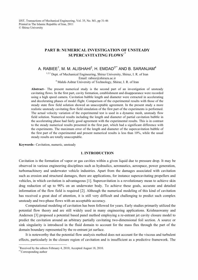
In this study, the flow about the model with spherical nose that was used in the experiments of part A will be numerically analyzed. Figure 1 depicts the model and with a solid modeler software, its mass and center of gravity are determined as 159.55(gram) and 6(cm) from the nose, respectively.

Fig. 1. Dimensions of the model are in millimeter

The unsteady supercavitating flow field can be studied with a variety of techniques. Commercial CFD software is used to simulate the two phase flow field that is explained in the following.

4. BODY MOTION ALONG WITH GRID In this method a grid is fixed around the body that follows the same movement of the body in every instant of the motion and the Navier-Stokes equations are solved in accelerating coordinates [24]. As the cells shape remains unvarying, this method is appropriate to solve the flow field about a single body. It must be noticed that at any time step the boundary conditions must be applied accurately, and appropriate terms should be added to the equations of fluid motion to compensate for non-inertial coordinate effects.

5. DYNAMIC MESH Dynamic mesh is one of the most popular methods to investigate the unsteady flow fields involving moving boundaries and objects, particularly those having simultaneous translational and angular velocity. This method can be implemented in the available software used in part A [16]. It is noteworthy that in our problem of a moving body in a stationary fluid, far field boundary conditions do not vary with time. However, the mesh should be regenerated to conform with new boundaries locations. The motion of the body can be either determined using a six degree of freedom software module or prescribed as an input in every time step.

In this technique, according to the new position of the body and the fixed outer boundaries, a new mesh is reconstructed either by moving the grid points or introducing and removing nodes. However, it should always be remembered that high mesh quality must be preserved in this process of remeshing. Upon solving the flow field equations in this new mesh, the unsteady flow field is marched in time.

Owing to the existence of high density ratios between different species (vapor and liquid) produced by the process of cavitation, usage of a suitable fine tuned numerical method is essential. In this regard, SIMPLEC algorithm for coupling pressure and velocity, and first order upwinding with adjusted under relaxation coefficients are used for discretization of all terms in the equations. In the following, the numerical steps to determine an unsteady dynamic mesh solution are explained.

A. Rabiee et al.


34

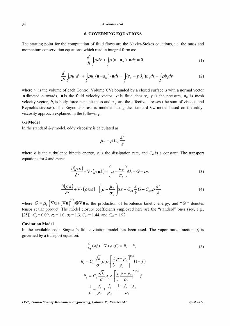
6. GOVERNING EQUATIONS The starting point for the computation of fluid flows are the Navier-Stokes equations, i.e. the mass and momentum conservation equations, which read in integral form as:

( ) 0mv s

d dv dsdt

ρ ρ+ − ⋅ =∫ ∫ u u n (1)

( ) ( )i i m ij ij j i

v s s v

d u dv u ds p n ds b dvdt

ρ ρ τ δ ρ+ − ⋅ = − +∫ ∫ ∫ ∫u u n (2)

where v is the volume of each Control Volume(CV) bounded by a closed surface s with a normal vector n directed outwards, u is the fluid velocity vector, ρ is fluid density, p is the pressure, um is mesh velocity vector, ib is body force per unit mass and ijτ are the effective stresses (the sum of viscous and Reynolds-stresses). The Reynolds-stress is modeled using the standard k-ε model based on the eddy-viscosity approach explained in the following. k-ε Model In the standard k-ε model, eddy viscosity is calculated as

ερμ μ

2kCT =

where k is the turbulence kinetic energy, ε is the dissipation rate, and Cμ is a constant. The transport equations for k and ε are:

( ) ( ) ρεσμμρρ

−+Δ⎟⎟⎠

⎞⎜⎜⎝

⎛+=⋅∇+

∂∂ Gkk

tk

k

Tu (3)

( ) ( )

kCG

kC

tT

2

21ερεε

σμ

μερερεε

ε

−+Δ⎟⎟⎠

⎞⎜⎜⎝

⎛+=⋅∇+

∂∂ u (4)

where ( )( )T

TG μ= ∇ + ∇ ⊗∇u u u is the production of turbulence kinetic energy, and “⊗ ” denotes tensor scalar product. The model closure coefficients employed here are the “standard” ones (see, e.g., [25]): Cμ = 0.09, σk = 1.0, σε = 1.3, Cε1 = 1.44, and Cε2 = 1.92. Cavitation Model In the available code Singual’s full cavitation model has been used. The vapor mass fraction, f, is governed by a transport equation:

ce RRfft

−=∇+∂∂ ).()( uρρ (5)

( )fppkCR

l

vvlee −⎥

⎦

⎤⎢⎣

⎡ −= 1

32

2/1

ρρρ

σ

fppkCR

l

vllcc

2/1

32

⎥⎦

⎤⎢⎣

⎡ −=

ρρρ

σ

l

gv

g

g

v

v ffffρρρρ−−

++=11



35

The source terms Re and Rc denote vapor generation evaporation and condensation rates, and can be functions of flow parameters (pressure, flow characteristic velocity) and fluid properties (liquid and vapor phase densities, saturation pressure, and liquid-vapor surface tension), where vρ , lρ , vp and gf are vapor density, liquid density, saturation pressure and mass fraction of non-condensable gas, respectively.

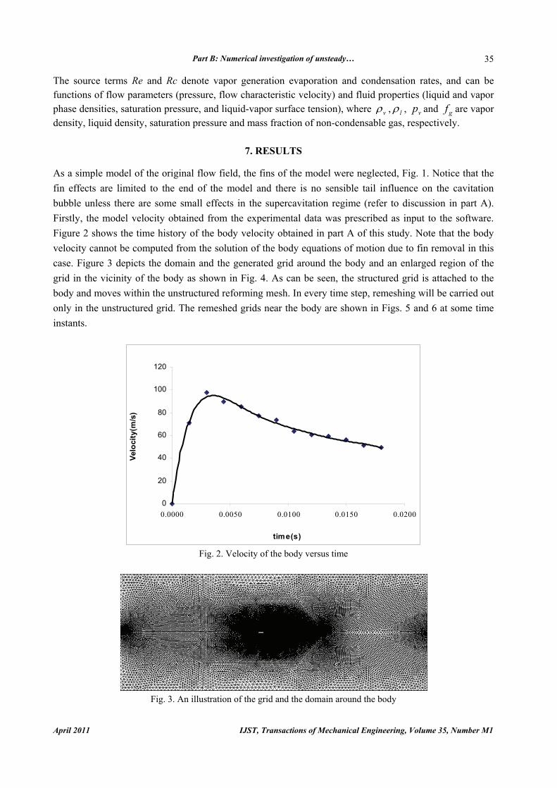
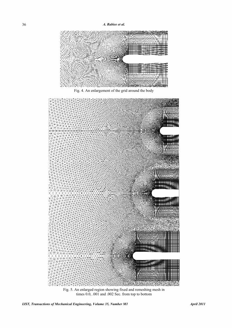
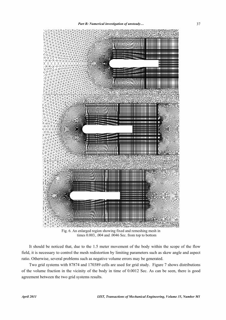
7. RESULTS As a simple model of the original flow field, the fins of the model were neglected, Fig. 1. Notice that the fin effects are limited to the end of the model and there is no sensible tail influence on the cavitation bubble unless there are some small effects in the supercavitation regime (refer to discussion in part A). Firstly, the model velocity obtained from the experimental data was prescribed as input to the software. Figure 2 shows the time history of the body velocity obtained in part A of this study. Note that the body velocity cannot be computed from the solution of the body equations of motion due to fin removal in this case. Figure 3 depicts the domain and the generated grid around the body and an enlarged region of the grid in the vicinity of the body as shown in Fig. 4. As can be seen, the structured grid is attached to the body and moves within the unstructured reforming mesh. In every time step, remeshing will be carried out only in the unstructured grid. The remeshed grids near the body are shown in Figs. 5 and 6 at some time instants.

0

20

40

60

80

100

120

0.0000 0.0050 0.0100 0.0150 0.0200

time(s)

Velo

city

(m/s

)

Fig. 2. Velocity of the body versus time

Fig. 3. An illustration of the grid and the domain around the body

A. Rabiee et al.


36

Fig. 4. An enlargement of the grid around the body

Fig. 5. An enlarged region showing fixed and remeshing mesh in

times 0.0, .001 and .002 Sec. from top to bottom



37

Fig. 6. An enlarged region showing fixed and remeshing mesh in

times 0.003, .004 and .0046 Sec. from top to bottom

It should be noticed that, due to the 1.5 meter movement of the body within the scope of the flow field, it is necessary to control the mesh redistortion by limiting parameters such as skew angle and aspect ratio. Otherwise, several problems such as negative volume errors may be generated.

Two grid systems with 87874 and 170389 cells are used for grid study. Figure 7 shows distributions of the volume fraction in the vicinity of the body in time of 0.0012 Sec. As can be seen, there is good agreement between the two grid systems results.

A. Rabiee et al.


38

0

0.2

0.4

0.6

0.8

1

1.2

-0.3 -0.25 -0.2 -0.15 -0.1 -0.05 0

L(m)

Phas

e-1

87874 cell170389 cell

Fig. 7. Distribution of volume fraction versus the axial length using two grid systems

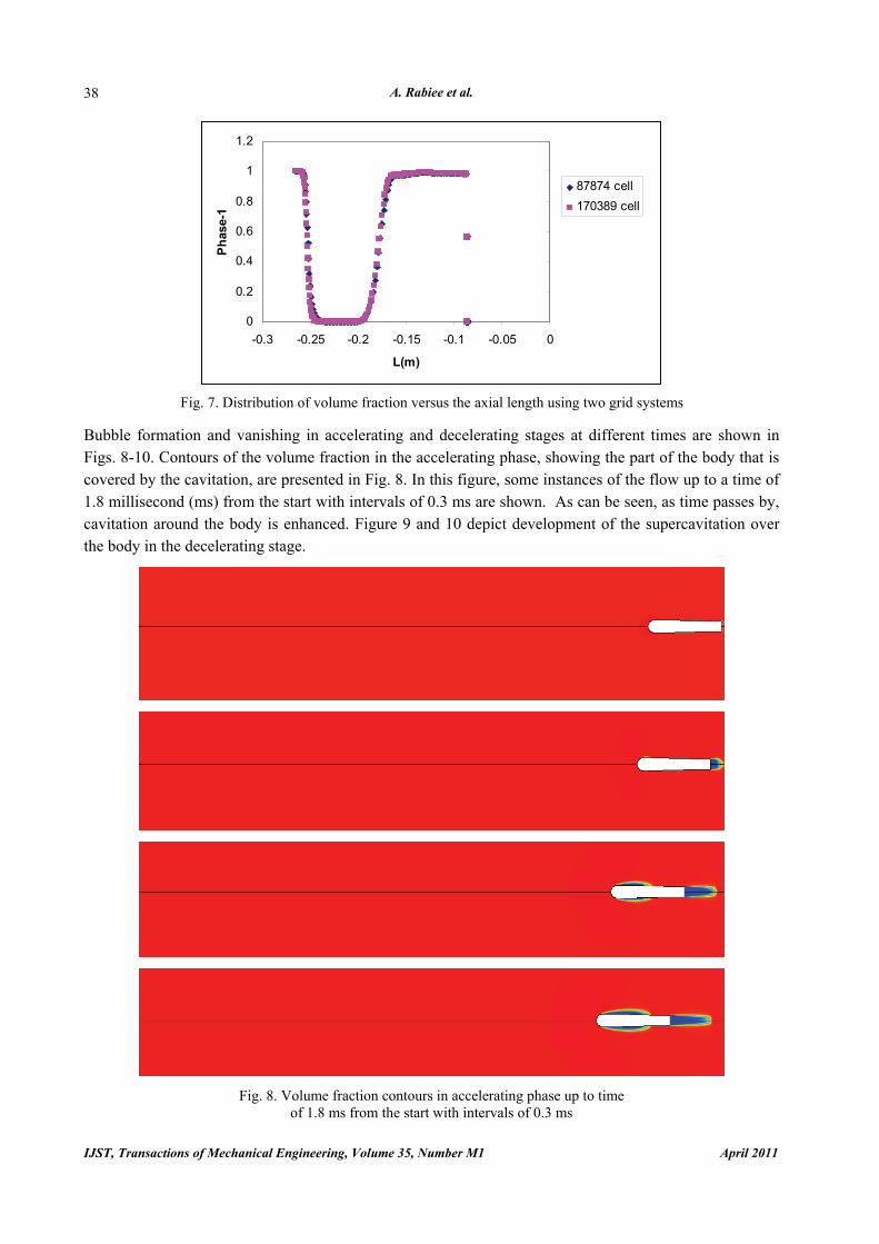
Bubble formation and vanishing in accelerating and decelerating stages at different times are shown in Figs. 8-10. Contours of the volume fraction in the accelerating phase, showing the part of the body that is covered by the cavitation, are presented in Fig. 8. In this figure, some instances of the flow up to a time of 1.8 millisecond (ms) from the start with intervals of 0.3 ms are shown. As can be seen, as time passes by, cavitation around the body is enhanced. Figure 9 and 10 depict development of the supercavitation over the body in the decelerating stage.

Fig. 8. Volume fraction contours in accelerating phase up to time

of 1.8 ms from the start with intervals of 0.3 ms



39

Fig. 8. Continued

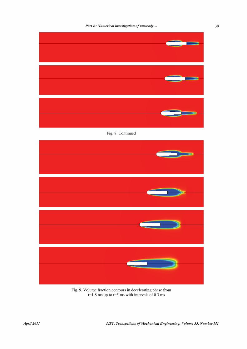
Fig. 9. Volume fraction contours in decelerating phase from

t=1.8 ms up to t=5 ms with intervals of 0.3 ms

A. Rabiee et al.


40

Fig. 9. Continued

Fig. 10. Volume fraction contours in decelerating phase from

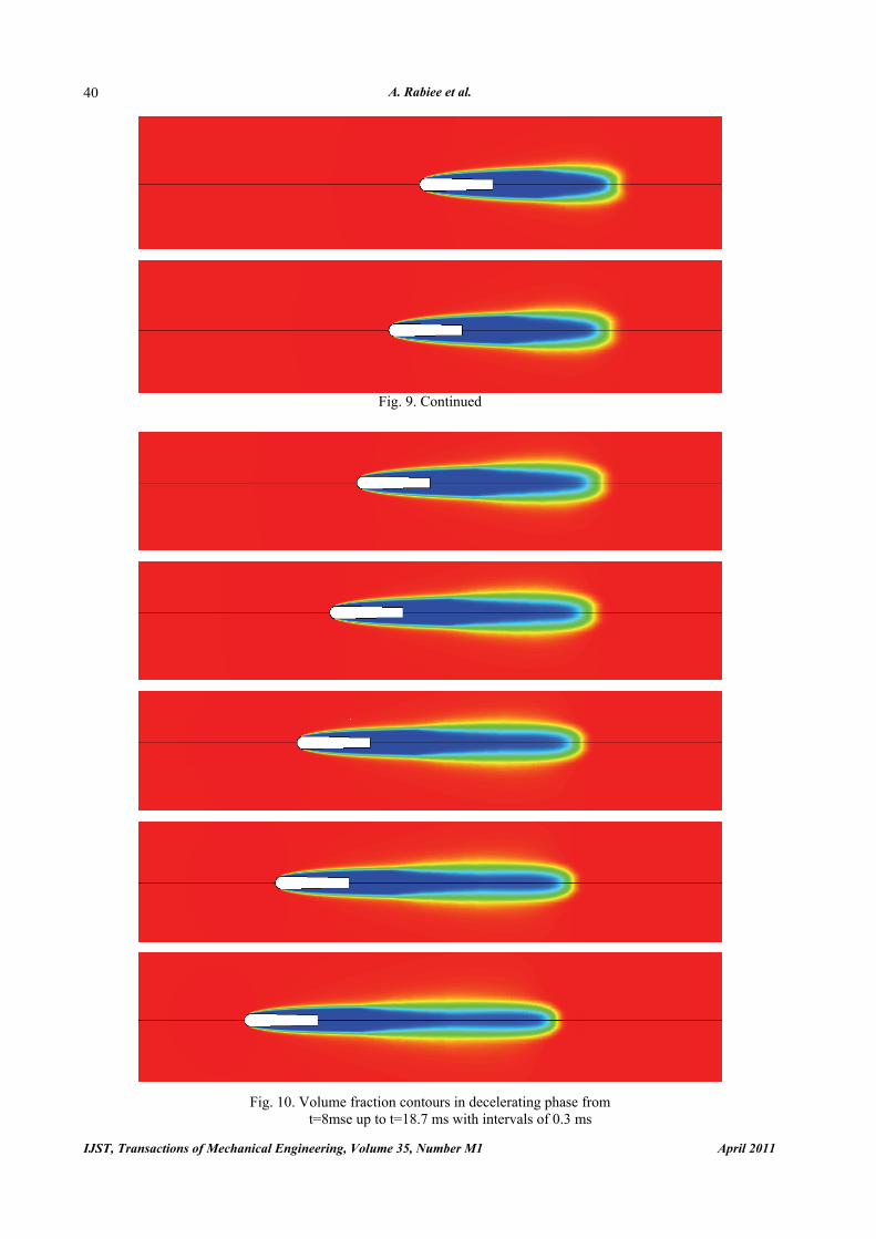
t=8mse up to t=18.7 ms with intervals of 0.3 ms



41

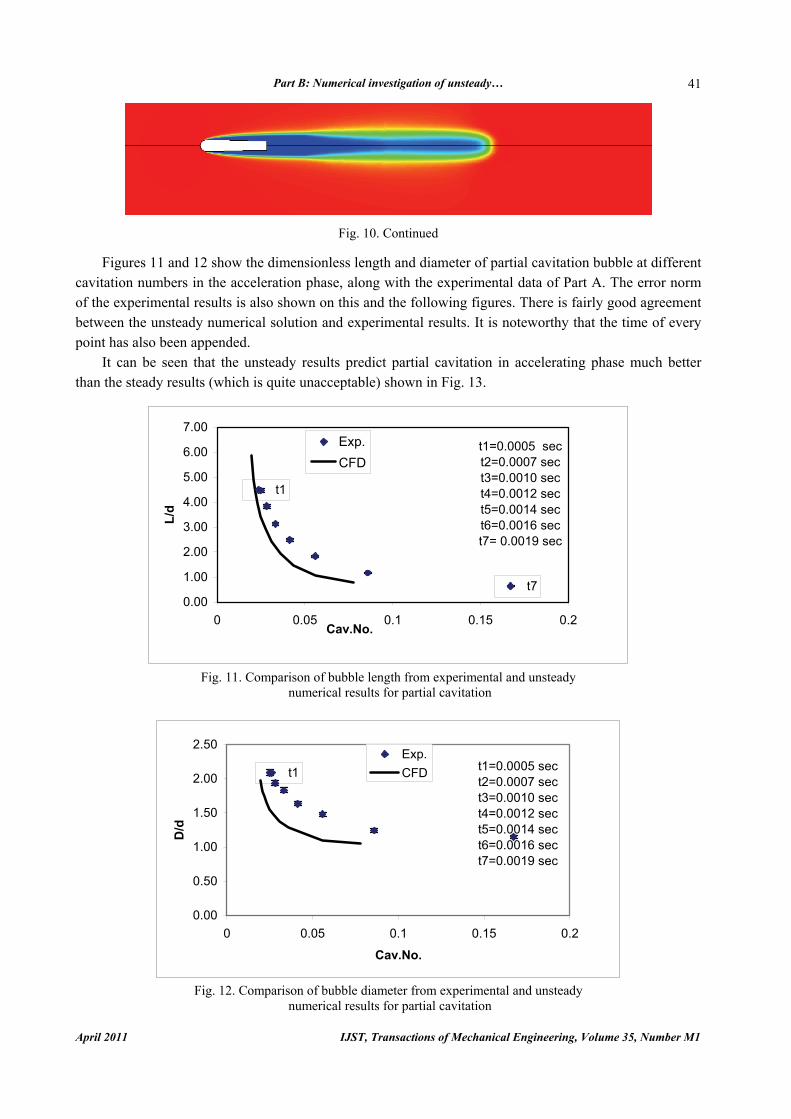
Fig. 10. Continued

Figures 11 and 12 show the dimensionless length and diameter of partial cavitation bubble at different

cavitation numbers in the acceleration phase, along with the experimental data of Part A. The error norm of the experimental results is also shown on this and the following figures. There is fairly good agreement between the unsteady numerical solution and experimental results. It is noteworthy that the time of every point has also been appended.

It can be seen that the unsteady results predict partial cavitation in accelerating phase much better than the steady results (which is quite unacceptable) shown in Fig. 13.

t1=0.0005 sect2=0.0007 sect3=0.0010 sect4=0.0012 sect5=0.0014 sect6=0.0016 sect7= 0.0019 sec

t1

t70.00

1.00

2.00

3.00

4.00

5.00

6.00

7.00

0 0.05 0.1 0.15 0.2Cav.No.

L/d

Exp.CFD

Fig. 11. Comparison of bubble length from experimental and unsteady

numerical results for partial cavitation

t1=0.0005 sect2=0.0007 sect3=0.0010 sect4=0.0012 sect5=0.0014 sect6=0.0016 sect7=0.0019 sec

t1

0.00

0.50

1.00

1.50

2.00

2.50

0 0.05 0.1 0.15 0.2

Cav.No.

D/d

Exp.CFD

Fig. 12. Comparison of bubble diameter from experimental and unsteady

numerical results for partial cavitation

A. Rabiee et al.


42

0.0

5.0

10.0

15.0

20.0

25.0

30.0

35.0

40.0

0.01 0.02 0.03 0.04 0.05

Cav.No.

L/d

Exp.Steady

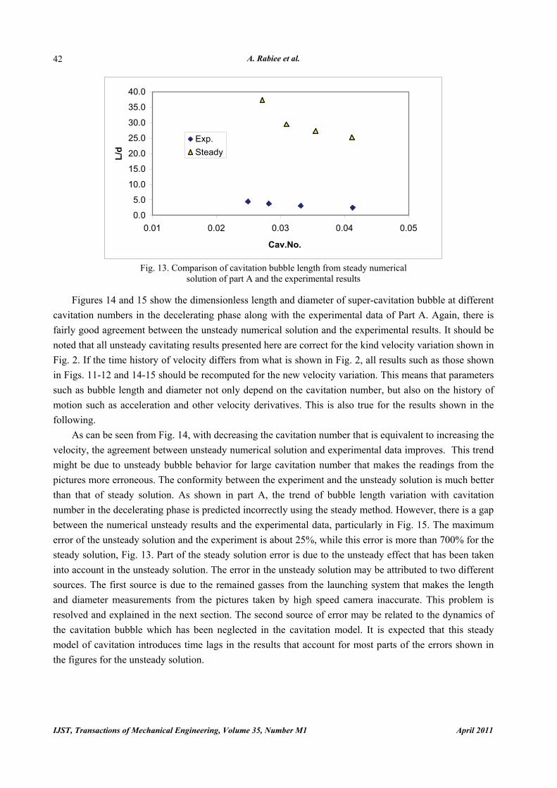
Fig. 13. Comparison of cavitation bubble length from steady numerical

solution of part A and the experimental results

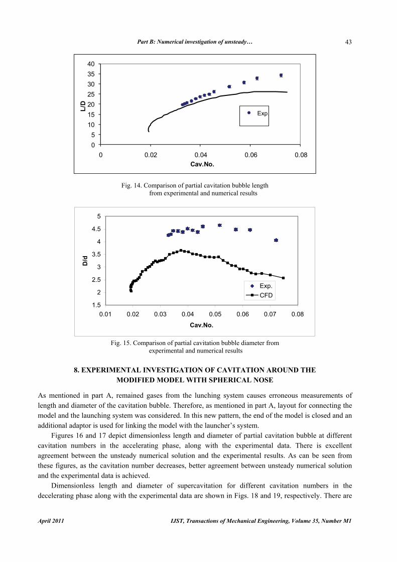
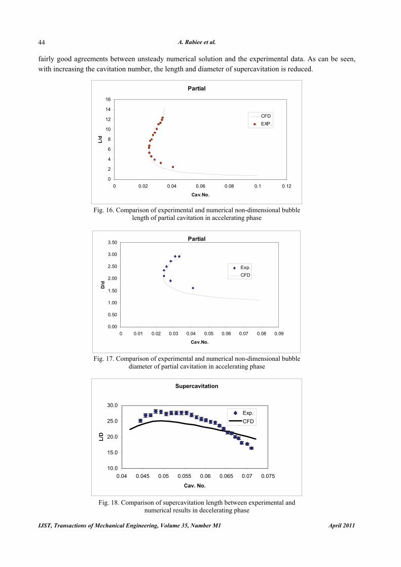
Figures 14 and 15 show the dimensionless length and diameter of super-cavitation bubble at different cavitation numbers in the decelerating phase along with the experimental data of Part A. Again, there is fairly good agreement between the unsteady numerical solution and the experimental results. It should be noted that all unsteady cavitating results presented here are correct for the kind velocity variation shown in Fig. 2. If the time history of velocity differs from what is shown in Fig. 2, all results such as those shown in Figs. 11-12 and 14-15 should be recomputed for the new velocity variation. This means that parameters such as bubble length and diameter not only depend on the cavitation number, but also on the history of motion such as acceleration and other velocity derivatives. This is also true for the results shown in the following.

As can be seen from Fig. 14, with decreasing the cavitation number that is equivalent to increasing the velocity, the agreement between unsteady numerical solution and experimental data improves. This trend might be due to unsteady bubble behavior for large cavitation number that makes the readings from the pictures more erroneous. The conformity between the experiment and the unsteady solution is much better than that of steady solution. As shown in part A, the trend of bubble length variation with cavitation number in the decelerating phase is predicted incorrectly using the steady method. However, there is a gap between the numerical unsteady results and the experimental data, particularly in Fig. 15. The maximum error of the unsteady solution and the experiment is about 25%, while this error is more than 700% for the steady solution, Fig. 13. Part of the steady solution error is due to the unsteady effect that has been taken into account in the unsteady solution. The error in the unsteady solution may be attributed to two different sources. The first source is due to the remained gasses from the launching system that makes the length and diameter measurements from the pictures taken by high speed camera inaccurate. This problem is resolved and explained in the next section. The second source of error may be related to the dynamics of the cavitation bubble which has been neglected in the cavitation model. It is expected that this steady model of cavitation introduces time lags in the results that account for most parts of the errors shown in the figures for the unsteady solution.



43

05

10152025303540

0 0.02 0.04 0.06 0.08

L/D

Cav.No.

Exp.

Fig. 14. Comparison of partial cavitation bubble length

from experimental and numerical results

1.5

2

2.5

3

3.5

4

4.5

5

0.01 0.02 0.03 0.04 0.05 0.06 0.07 0.08

Cav.No.

D/d

Exp.CFD

Fig. 15. Comparison of partial cavitation bubble diameter from

experimental and numerical results

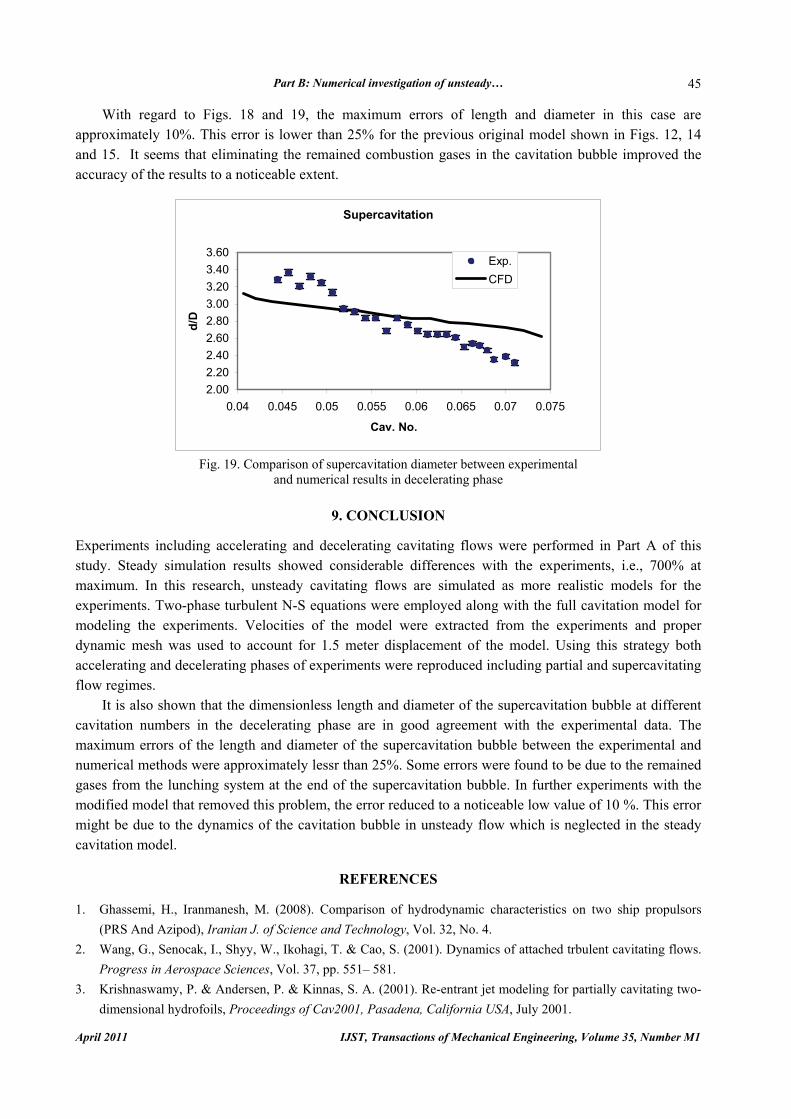
8. EXPERIMENTAL INVESTIGATION OF CAVITATION AROUND THE MODIFIED MODEL WITH SPHERICAL NOSE

As mentioned in part A, remained gases from the lunching system causes erroneous measurements of length and diameter of the cavitation bubble. Therefore, as mentioned in part A, layout for connecting the model and the launching system was considered. In this new pattern, the end of the model is closed and an additional adaptor is used for linking the model with the launcher’s system.

Figures 16 and 17 depict dimensionless length and diameter of partial cavitation bubble at different cavitation numbers in the accelerating phase, along with the experimental data. There is excellent agreement between the unsteady numerical solution and the experimental results. As can be seen from these figures, as the cavitation number decreases, better agreement between unsteady numerical solution and the experimental data is achieved.

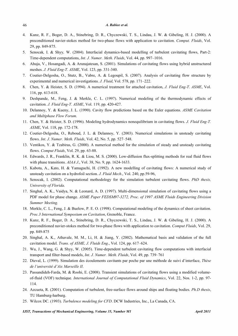
Dimensionless length and diameter of supercavitation for different cavitation numbers in the decelerating phase along with the experimental data are shown in Figs. 18 and 19, respectively. There are

A. Rabiee et al.


44

fairly good agreements between unsteady numerical solution and the experimental data. As can be seen, with increasing the cavitation number, the length and diameter of supercavitation is reduced.

Partial

0

2

4

6

8

10

12

14

16

0 0.02 0.04 0.06 0.08 0.1 0.12

Cav.No.

L/d

CFDEXP.

Fig. 16. Comparison of experimental and numerical non-dimensional bubble

length of partial cavitation in accelerating phase

Partial

0.00

0.50

1.00

1.50

2.00

2.50

3.00

3.50

0 0.01 0.02 0.03 0.04 0.05 0.06 0.07 0.08 0.09

Cav.No.

D/d

Exp.CFD

Fig. 17. Comparison of experimental and numerical non-dimensional bubble

diameter of partial cavitation in accelerating phase

Supercavitation

10.0

15.0

20.0

25.0

30.0

0.04 0.045 0.05 0.055 0.06 0.065 0.07 0.075

Cav. No.

L/D

Exp.CFD

Fig. 18. Comparison of supercavitation length between experimental and

numerical results in decelerating phase



45

With regard to Figs. 18 and 19, the maximum errors of length and diameter in this case are approximately 10%. This error is lower than 25% for the previous original model shown in Figs. 12, 14 and 15. It seems that eliminating the remained combustion gases in the cavitation bubble improved the accuracy of the results to a noticeable extent.

Supercavitation

2.002.202.402.602.803.003.203.403.60

0.04 0.045 0.05 0.055 0.06 0.065 0.07 0.075

Cav. No.

d/D

Exp.CFD

Fig. 19. Comparison of supercavitation diameter between experimental

and numerical results in decelerating phase

9. CONCLUSION Experiments including accelerating and decelerating cavitating flows were performed in Part A of this study. Steady simulation results showed considerable differences with the experiments, i.e., 700% at maximum. In this research, unsteady cavitating flows are simulated as more realistic models for the experiments. Two-phase turbulent N-S equations were employed along with the full cavitation model for modeling the experiments. Velocities of the model were extracted from the experiments and proper dynamic mesh was used to account for 1.5 meter displacement of the model. Using this strategy both accelerating and decelerating phases of experiments were reproduced including partial and supercavitating flow regimes.

It is also shown that the dimensionless length and diameter of the supercavitation bubble at different cavitation numbers in the decelerating phase are in good agreement with the experimental data. The maximum errors of the length and diameter of the supercavitation bubble between the experimental and numerical methods were approximately lessr than 25%. Some errors were found to be due to the remained gases from the lunching system at the end of the supercavitation bubble. In further experiments with the modified model that removed this problem, the error reduced to a noticeable low value of 10 %. This error might be due to the dynamics of the cavitation bubble in unsteady flow which is neglected in the steady cavitation model.

REFERENCES 1. Ghassemi, H., Iranmanesh, M. (2008). Comparison of hydrodynamic characteristics on two ship propulsors

(PRS And Azipod), Iranian J. of Science and Technology, Vol. 32, No. 4. 2. Wang, G., Senocak, I., Shyy, W., Ikohagi, T. & Cao, S. (2001). Dynamics of attached trbulent cavitating flows.

Progress in Aerospace Sciences, Vol. 37, pp. 551– 581. 3. Krishnaswamy, P. & Andersen, P. & Kinnas, S. A. (2001). Re-entrant jet modeling for partially cavitating two-

dimensional hydrofoils, Proceedings of Cav2001, Pasadena, California USA, July 2001.

A. Rabiee et al.


46

4. Kunz, R. F., Boger, D. A., Stinebring, D. R., Chyczewski, T. S., Lindau, J. W. & Gibeling, H. J. (2000). A preconditioned navier-stokes method for two-phase flows with application to cavitation. Comput. Fluids, Vol. 29, pp. 849-875.

5. Senocak, I. & Shyy, W. (2004). Interfacial dynamics-based modelling of turbulent cavitating flows, Part-2: Time-dependent computations, Int. J. Numer. Meth. Fluids, Vol. 44, pp. 997–1016.

6. Ahuja, V., Hosangadi, A. & Arunajatesan, S. (2001). Simulations of cavitating flows using hybrid unstructured meshes. J. Fluid Eng-T. ASME, Vol. 123, pp. 331-340.

7. Coutier-Delgosha, O., Stutz, B., Vabre, A. & Legoupil, S. (2007). Analysis of cavitating flow structure by experimental and numerical investigations. J. Fluid, Vol. 578, pp. 171–222.

8. Chen, Y. & Heister, S. D. (1994). A numerical treatment for attached cavitation, J. Fluid Eng-T. ASME, Vol. 116, pp. 613-618.

9. Deshpande, M., Feng, J. & Merkle, C. L. (1997). Numerical modeling of the thermodynamic effects of cavitation. J. Fluid Eng-T. ASME, Vol. 119, pp. 420-427.

10. Delannoy, Y. & Kueny, J. L. (1990). Cavity flow predictions based on the Euler equations. ASME Cavitation and Multiphase Flow Forum.

11. Chen, Y. & Heister, S. D. (1996). Modeling hydrodynamics nonequilibrium in cavitating flows. J. Fluid Eng-T. ASME, Vol. 118, pp. 172-178.

12. Coutier-Delgosha, O., Reboud, J. L. & Delannoy, Y. (2003). Numerical simulations in unsteady cavitating flows. Int. J. Numer. Meth. Fluids, Vol. 42, No. 5, pp. 527–548.

13. Ventikos, Y. & Tzabiras, G. (2000). A numerical method for the simulation of steady and unsteady cavitating flows. Comput Fluids, Vol. 29, pp. 63-88.

14. Edwards, J. R., Franklin, R. K. & Liou, M. S. (2000). Low-diffusion flux-splitting methods for real fluid flows with phase transitions. AIAA J., Vol. 38, No. 9, pp. 1624-1633.

15. Kubota, A., Kato, H. & Yamaguchi, H. (1992). A new modelling of cavitating flows: A numerical study of unsteady cavitation on a hydrofoil section. J. Fluid Mech., Vol. 240, pp.59-96,

16. Senocak, I. (2002). Computational methodology for the simulation turbulent cavitating flows. PhD thesis, University of Florida.

17. Singhal, A. K., Vaidya, N. & Leonard, A. D. (1997). Multi-dimensional simulation of cavitating flows using a PDF model for phase change. ASME Paper FEDSM97-3272, Proc. of 1997 ASME Fluids Engineering Division Summer Meeting.

18. Merkle, C. L., Feng, J. & Buelow, P. E. O. (1998). Computational modeling of the dynamics of sheet cavitation. Proc.3 International Symposium on Cavitation, Grenoble, France.

19. Kunz, R. F., Boger, D. A., Stinebring, D. R., Chyczewski, T. S., Lindau, J. W. & Gibeling, H. J. (2000). A preconditioned navier-stokes method for two-phase flows with application to cavitation. Comput Fluids, Vol. 29, pp. 849-875

20. Singhal, A. K., Athavale, M. M., Li, H. & Jiang, Y. (2002). Mathematical basis and validation of the full cavitation model. Trans. of ASME, J. Fluids Eng., Vol. 124, pp. 617–624.

21. Wu, J., Wang, G. & Shyy, W. (2005). Time-dependent turbulent cavitating flow computations with interfacial transport and filter-based models, Int. J. Numer. Meth. Fluids, Vol. 49, pp. 739–761

22. Dieval, L. (1999). Simulation des écoulements cavitants par poche par une méthode de suivi d’interface, Thèse de l’université d’Aix Marseille II.

23. Passandideh-Farda, M. & Roohi, E. (2008). Transient simulations of cavitating flows using a modified volume-of-fluid (VOF) technique. International Journal of Computational Fluid Dynamics, Vol. 22, Nos. 1-2, pp. 97-114.

24. Azcueta, R. (2001). Computation of turbulent, free-surface flows around ships and floating bodies. Ph.D thesis, TU Hamburg-harburg.

25. Wilcox DC. (1993). Turbulence modeling for CFD. DCW Industries, Inc., La Canada, CA.

PART B: NUMERICAL INVESTIGATION OF UNSTEADY...

Documents

Transcript of PART B: NUMERICAL INVESTIGATION OF UNSTEADY...