PART 2: Statistical Pattern Classification: Optimal Classification with Bayes Rule METU Informatics...
34
PART 2: Statistical Pattern Classification: Optimal Classification with Bayes Rule METU Informatics Institute Min 720 Pattern Classification with Bio-Medical Applications
-
Upload
pierce-williams -
Category
Documents
-
view
227 -
download
1
Transcript of PART 2: Statistical Pattern Classification: Optimal Classification with Bayes Rule METU Informatics...
PART 2: Statistical Pattern Classification: Optimal Classification with Bayes Rule
METU Informatics Institute Min 720 Pattern Classification with Bio-Medical Applications

Statistical Approach to P.R
Dimension of the feature space:Set of different states of nature:Categories:find
set of possible actions (decisions): Here, a decision might include a ‘reject option’ A Discriminant Function
in region ; decision rule : if
],...,,[ 21 dXXXX
d
},...,,{ 21 c
c
iR ji RR di RuR
},...,,{ 21 a
)()( XgXg ji
iR
)(Xg i ci 1
k )()( XgXg jk
1R1g
2g2R
3R3g

A Pattern Classifier
So our aim now will be to define these functionsto minimize or optimize a criterion.
)(1 Xg
X
)(Xgc
)(2 Xg Max
cggg ,...,, 21
k
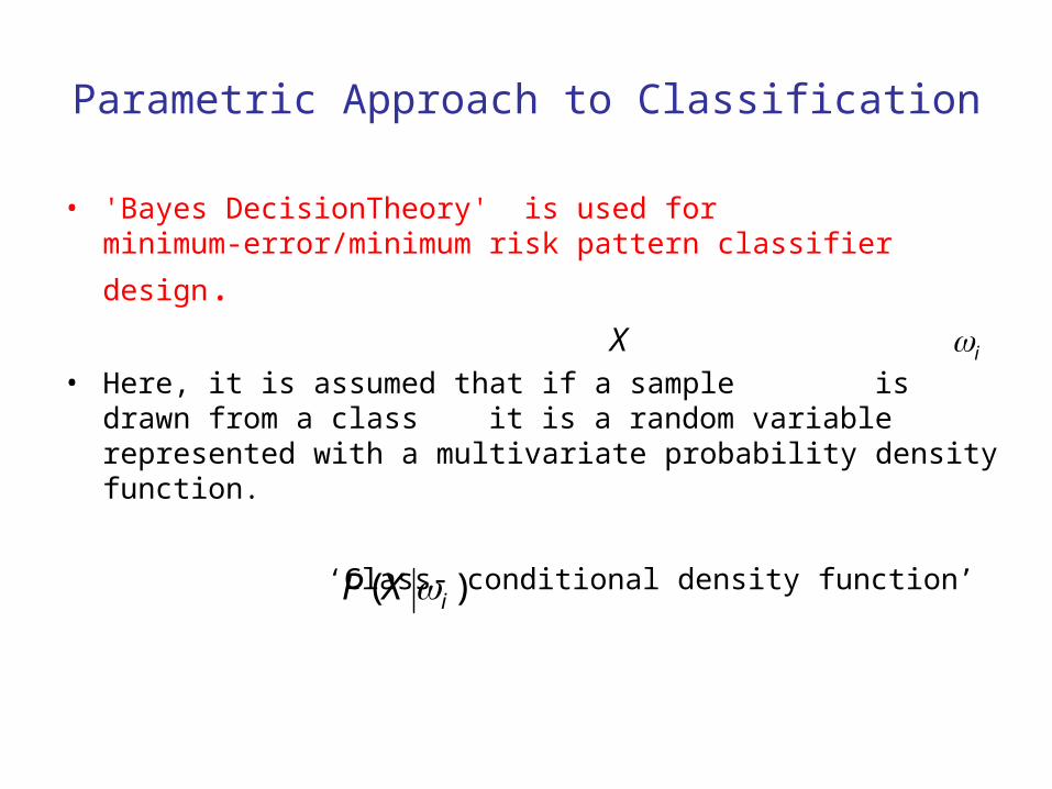
Parametric Approach to Classification
• 'Bayes DecisionTheory' is used for minimum-error/minimum
risk pattern classifier design.
• Here, it is assumed that if a sample is drawn from a class it is a random variable represented with a multivariate probability density function.
‘Class- conditional density function’
X i
)( iXP

• We also know a-priori probability
• (c is no. of classes)
• Then, we can talk about a decision rule that minimizes the probability of error.
• Suppose we have the observation • This observation is going to change a-priori assumption to a-
posteriori probability:
• which can be found by the Bayes Rule.
)( XP i
ci 1)( iP
X
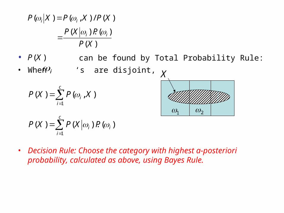
• can be found by Total Probability Rule:
• When ‘s are disjoint,
• Decision Rule: Choose the category with highest a-posteriori probability, calculated as above, using Bayes Rule.
)(/),()( XPXPXP ii
c
iii PXPXP
1
)().()(
X
21
)(
)().(
XP
PXP ii
)(XP
i
c
ii XPXP
1
),()(

• then, 1
• Decision boundary:
• or in general, decision boundaries are where:
• between regions and
2R1R
21 gg
)()( XPXg ii
21 gg
12 gg
)()( XgXg ji iR jR
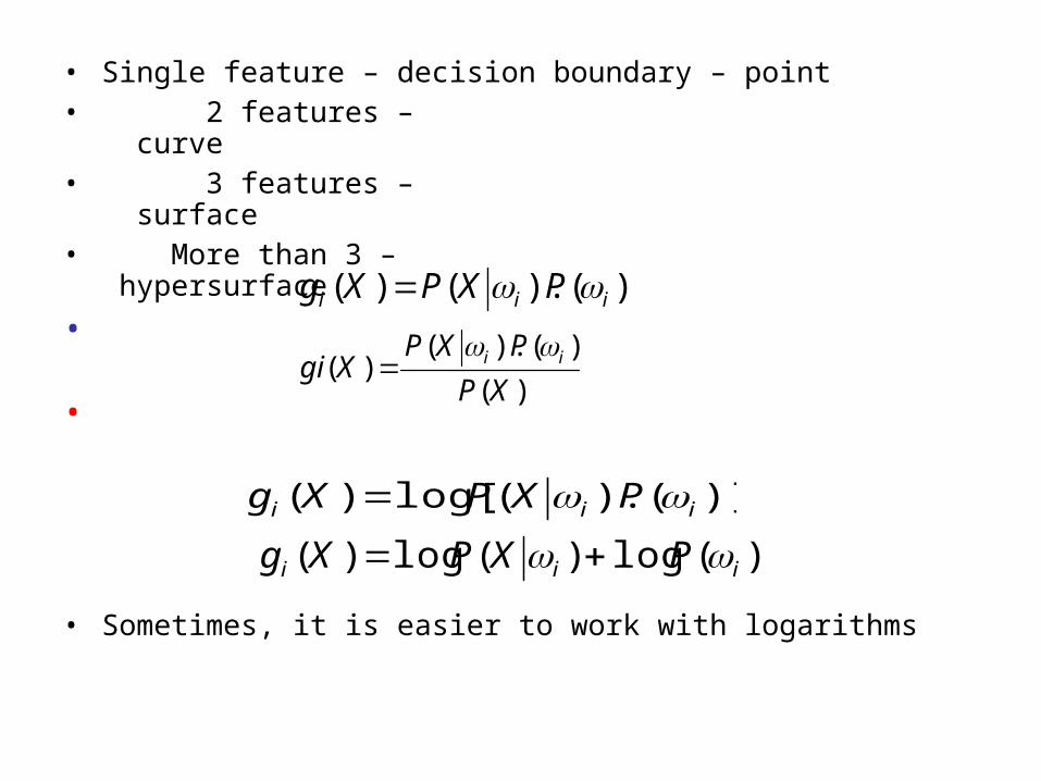
• Single feature – decision boundary – point • 2 features – curve • 3 features – surface • More than 3 – hypersurface
• •
• Sometimes, it is easier to work with logarithms
• Since logarithmic function is a monotonically increasing function, log fn will give the same result.
)().()( iii PXPXg
)]().(log[)( iii PXPXg
)(log)(log)( iii PXPXg
)(
)().()(
XP
PXPXgi ii
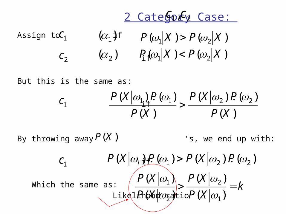
2 Category Case:
Assign to if if
But this is the same as: if
By throwing away ‘s, we end up with:
if
Which the same as: Likelihood ratio
kXP
XP
XP
XP)(
)(
)(
)(
1
2
2
1
21,cc
1c )()( 21 XPXP
2c
)().()().( 221 PXPPXP i
)(XP
)(
)().(
)(
)().( 2211
XP
PXP
XP
PXP 1c
)()( 21 XPXP
1c
)( 2
)( 1
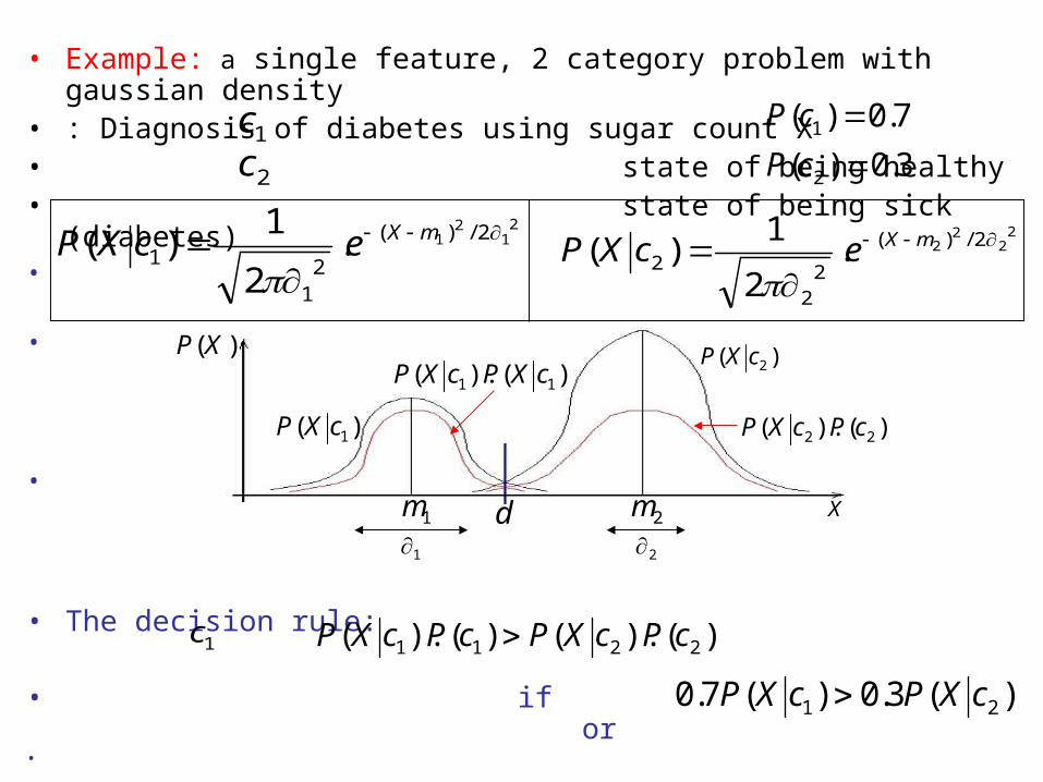
• Example: a single feature, 2 category problem with gaussian density
• : Diagnosis of diabetes using sugar count X• state of being healthy• state of being sick (diabetes)•
•
•
• The decision rule:
• if or•
)().()().( 2211 cPcXPcPcXP
1c 7.0)( 1 cP
2c
22
22 2/)(
22
2 .2
1)(
mXecXP
)(3.0)(7.0 21 cXPcXP
21
21 2/)(
21
1 .2
1)(
mXecXP
X
3.0)( 2 cP
1c
1m
)(XP
21
)( 2cXP
)().( 22 cPcXP
)().( 11 cXPcXP
)( 1cXP
d 2m
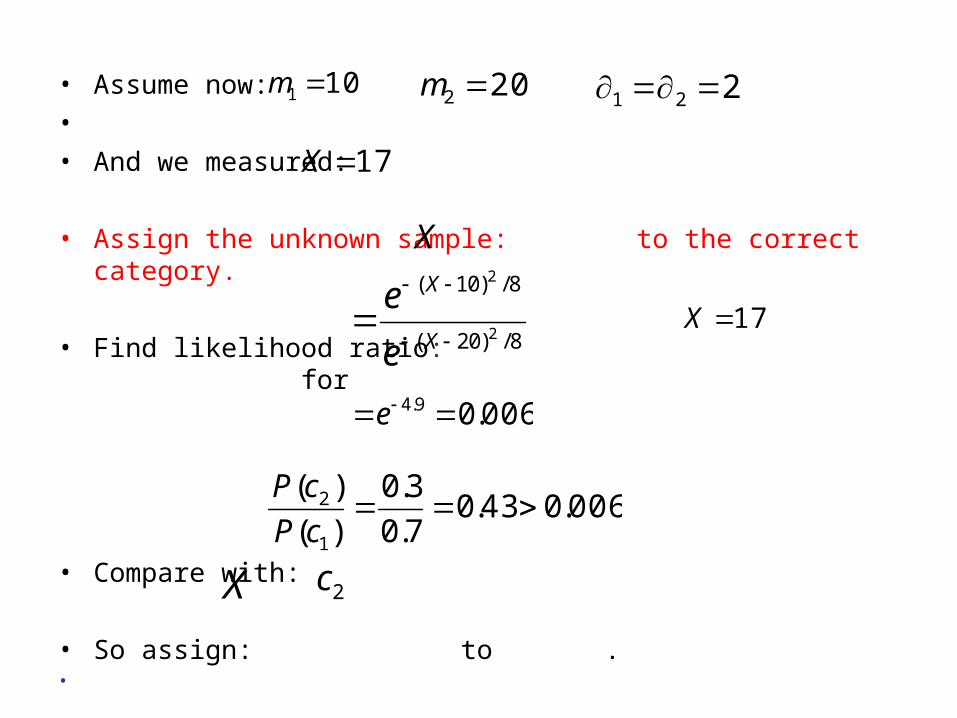
• Assume now: • • And we measured:
• Assign the unknown sample: to the correct category.
• Find likelihood ratio: for
• Compare with:
• So assign: to .•
17X
101 m 202 m
006.043.07.0
3.0
)(
)(
1
2 cP
cP
006.09.4 e
8/)20(
8/)10(
2
2
X
X
e
e
2cX
221
17X
X

• Example: A discrete problem• Consider a 2-feature, 3 category case
• where:•
• And , ,• • Find the decision boundaries and regions:•
• Solution:•
•
• •
1.0)4.0(4
1
2.0)( 3 cP
ii bXa 1
4.0)( 1 cP
ii bXa 2
0
)(
1
),( 221 iii bacXXP
3
1R
4.0)( 2 cP
3
4
5.3
1
3
2
1
b
b
b
3
5.0
1
3
2
1
a
a
a
3R
9
4.04.0
9
1
for
1
wiseother
2.02.01
2R

• Remember now that for the 2-class case:• • if • • or•
Likelihood ratio
• • • Error probabilities and a simple proof of minimum error
• Consider again a 2-class 1-d problem:
•
• • • Let’s show that: if the decision boundary is (intersection
point) • rather than any arbitrary point .
•
)().( 11 cPcXP
d
)2().2()1().1( cPcXPcPcXP
1R
1c
d
d
)().( 22 cPcXP
d2R
kcXP
cXP
cXP
cXP)(
)(
)(
)(
1
2
2
1
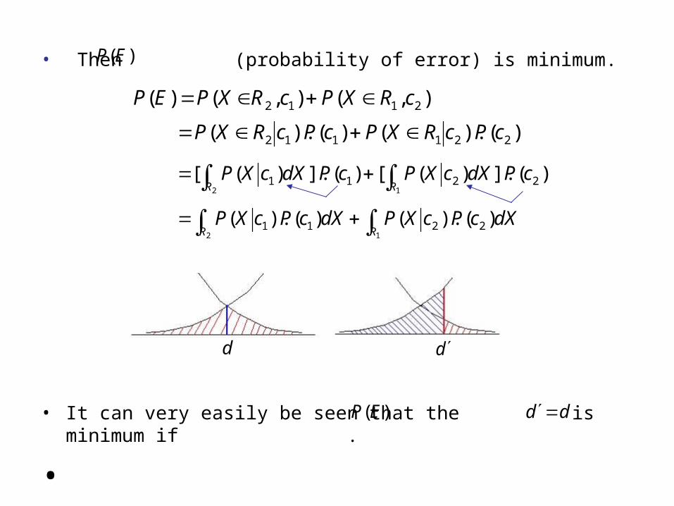
• Then (probability of error) is minimum.
• It can very easily be seen that the is minimum if .
•
12
)().()().( 2211 RRdXcPcXPdXcPcXP
)(EP
)().()().( 221112 cPcRXPcPcRXP
),(),()( 2112 cRXPcRXPEP
2 1
)(].)([)(].)([ 2211R RcPdXcXPcPdXcXP
dd )(EP
d d

Minimum Risk Classification Risk associated with incorrect decision might be more important
than the probability of error. So our decision criterion might be modified to minimize the
average risk in making an incorrect decision. We define a conditional risk (expected loss) for decision when
occurs as:
Where is defined as the conditional loss associated with decision when the true class is . It is assumed that is known.
The decision rule: decide on if for all
The discriminant function here can be defined as: 4
i X
)()( XRXg ii
ji cj 1)()( XRXR ji ic
ji
)( ji
c
jjji
i XPXR1
)().()(
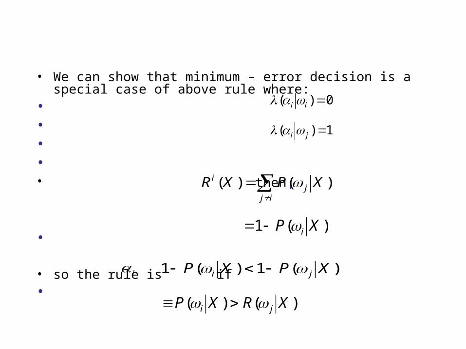
• We can show that minimum – error decision is a special case of above rule where:
• • • • • then,
•
• so the rule is if•
0)( ii
1)( ji
)()( XRXP ji
)(1 XP i
i )(1)(1 XPXP ji
ij
ji XPXR )()(
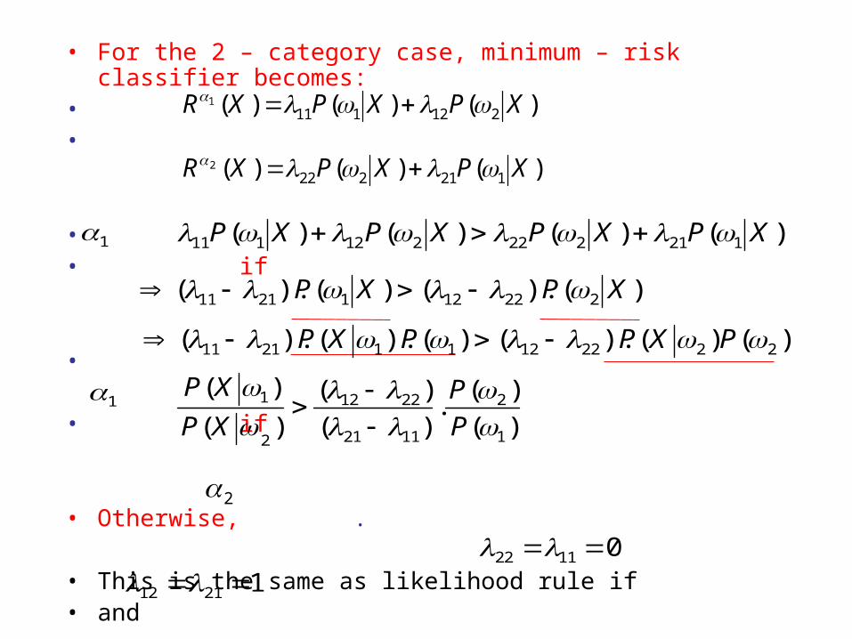
• For the 2 – category case, minimum – risk classifier becomes:
• •
• • if
•
• if
• Otherwise, .
• This is the same as likelihood rule if• and
)()()( 2121111 XPXPXR
1 )()()()( 121222212111 XPXPXPXP
)()()( 1212222 XPXPXR
)().()().( 2221212111 XPXP
)()().()().().( 222212112111 PXPPXP
1)(
)(.)(
)(
)(
)(
1
2
1121
2212
2
1
P
P
XP
XP
2
01122 12112

Discriminant Functions so far
For Minimum Error:
For Minimum Risk:
Where
)(log)(log
)().(
)(
ii
ii
i
PXP
PXP
XP
)(XR i
c
jjji
i XPXR1
)().()(

Bayes (Maximum Likelihood)Decision:
• Most general optimal solution• Provides an upper limit(you cannot do better with
other rule)• Useful in comparing with other classifiers

Special Cases of Discriminant Functions
Multivariate Gaussian (Normal) Density :
The general density form: Here in the feature vector of size . M : d element mean vector
: covariance matrix (variance of feature ) - symmetric when and are statistically independent.
d
dxd
jX
),( MN
iX
TdMXE ],...,,[)( 21
X
2i
])[(
)])([(2
iiii
jjiiij
XE
XXE
1
)()(2/1
2/12/)2(
1)(
MXMX
d
T
eXP
iX0ij

• - determinant of
•General shape: Hyper ellipsoids where
• is constant:• Mahalanobis
Distance • •
• 2 – d problem: ,
• If ,• (statistically independent features) then,• major axes are parallel to major ellipsoid axes
•
21, XX2X
1X
021 012
2221
1221
2
1
M
1)()( MXMX T
2X1X
2
1

•
• if in addition• circular
• in general, the equal density curves are hyper ellipsoids. Now
• is used for since its ease in manipulation
•
• is a quadratic function of as will be shown.
22
21
),( iiMN
X
2
1
)(loglog)2/1(
)()).(2/1()(1
ii
i iT
ii
P
MXMXXg
)(Xgi
)(log)(log)( ieiei PXPXg

a scalarThen,
On the decision boundary,
)(loglog.2/1
2/1.2/1
.2/1.2/1)(
1
11
11
ii
i
Tiii
T
i iTii
Ti
P
XMMX
MMXXXg
)(loglog.2/1.2/1
.2/1
1
1
1
iiiiTiio
i
Tii
ii
PMMW
MV
W
ioiiT
i WXVXWXXg )(
0
)()(
joiojijT
iT
ji
WWXVXVXWXXWX
XgXg

Decision boundary function is hyperquadratic in general.Example in 2d.
Then, above boundary becomes
0
0)()()(
0
WVXWXX
WWXVVXWWXT
joiojijiT
21
21
2221
1211
xxX
vvV
W

General form of hyper quadratic boundary IN 2-d.The special cases of Gaussian: AssumeWhere is the unit matrixIi
2
02 0221122222112
2111 Wxvxvxxxx
002
121
2
1
2221
121121
W
x
xvv
x
xxx
I
2
2
2
2
000
0..00
000
000
i
di
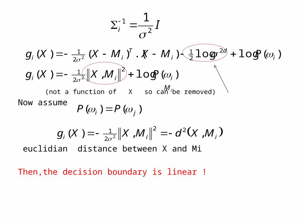
(not a function of X so can be removed)
Now assume
euclidian distance between X and Mi
Then,the decision boundary is linear !
iM
Ii 21 1
iii MXdMXXg ,,)( 22
212
)()( ji PP
)(log,)(
)(loglog).()()(2
21
221
21
2
2
iii
id
iT
ii
PMXXg
PMXMXXg
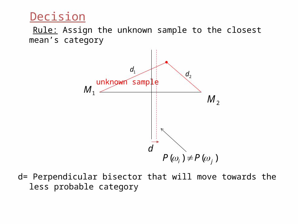
Decision
Rule: Assign the unknown sample to the closest mean’s category
unknown sample
d= Perpendicular bisector that will move towards the less probable category
2d
d
1M2M
)()( ji PP
1d

Minimum Distance Classifier
• Classify an unknown sample X to the category with closest mean !
• Optimum when gaussian densities with equal variance and equal a-priori probability.
Piecewise linear boundary in case of more than 2 categories.
1M
4R
2R
3R
4M
3M
2M1R

• Another special case: It can be shown that when (Covariance matrices are the same)
• Samples fall in clusters of equal size and shape unknown sample
is called Mahalonobis Distance
is called Mahalonobis Distance
)()( ji PP
)()(
)(log)()()(
121
121
iT
i
iiT
ii
MXMX
PMXMXXg
i
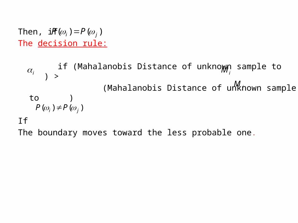
Then, if The decision rule:
if (Mahalanobis Distance of unknown sample to ) > (Mahalanobis Distance of unknown sample to )
IfThe boundary moves toward the less probable one.
i
)()( ji PP
)()( ji PP
jM
iM
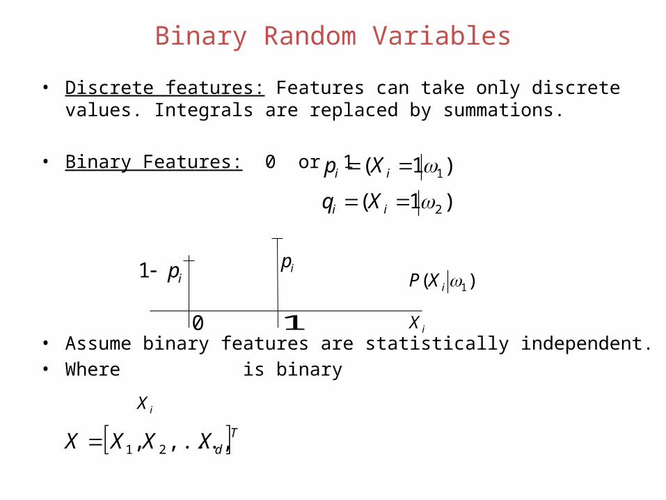
Binary Random Variables
• Discrete features: Features can take only discrete values. Integrals are replaced by summations.
• Binary Features: 0 or 1
• Assume binary features are statistically independent.• Where is binary
)1(
)1(
2
1
ii
ii
Xq
Xp
)( 1iXP
iX
TdXXXX ,...,, 21
ipip1
0 1 iX

Binary Random Variables
Example: Bit – matrix for machine – printed characters
a pixel
Here, each pixel may be taken as a feature For above problem, we have
is the probability that for letter A,B,…
iX
1iX
1001010 d
1
0
ip
iX
AB

defined for undefined elsewhere:
• If statistical independence of features is assumed.
• Consider the 2 category problem; assume:
d
ikiiiikkk
xi
xi
d
ii
d
i
i
xi
xii
wPpxpxwPwXPXg
ppxPXP
x
ppxP
ii
ii
1
1
11
1
)(log)1log()1(log))(log)(log()(
)1()()()(
1,0
)1()()(
)1(
)1(
2
1
xq
xp
i
i

then, the decision boundary is:
So if
The decision boundary is linear in X. a weighted sum of the inputs where:
and
0)( WXWXg ii
2
10
loglog)1(log
0)(log)(log
)1log()1(log)1log()1(log
)()(
11
21
2
1
else
category
xx
PP
qxqxpxpx
PP
qp
iqp
i
iiiiiiii
i
i
i
i
)()(
11
0 2
1lnln
PP
qp
i
iW)1()1(lnii
ii
pqqP
iW