Matthew Rose - Downer & Daniel Caldwell - WSP Parsons Brinkerhoff

August 2015
SMALL-SCALE GENERATION COST
UPDATE
Department of Energy and Climate Change
3514055AFinal


Small-scale Generation CostUpdate
3514055A
Prepared forDepartment of Energy and Climate Change
3 Whitehall PlaceLondon
SW1A 2AW
Prepared byParsons Brinckerhoff
Amber CourtWilliam Armstrong Drive
Newcastle upon TyneNE4 7YQ
0191 226 2654www.pbworld.com


Small-scale Generation Cost Update
DECC Small-Scale Generation Costs Update V11 - FINAL.docx Prepared by Parsons BrinckerhoffAugust 2015 for Department of Energy and Climate Change
- 5 -
CONTENTSPage
1 Scope of work 71.2 Stakeholder Engagement 71.3 Confidence 81.4 Data Adjustment 81.5 Consistency 8
2 Technology inputs 102.1 Approach and Methodology 102.2 Solar PV 142.3 Wind 232.4 Hydro 332.5 Anaerobic Digestion 392.6 Micro CHP 45
3 Review of Other inputs 473.2 Grid Connection Costs 473.3 Feedstock Types, Costs and Gate Fees – Anaerobic Digestion 493.4 Evolution of Feedstock Costs and Gate Fees – Anaerobic Digestion 523.5 Digestate Disposal – Anaerobic Digestion 533.6 Anti-dumping scenarios – Solar PV 54
4 Qualitative assessment 584.1 Introduction 584.2 Solar – domestic 584.3 Solar – commercial 584.4 Wind 594.5 Hydro 614.6 Anaerobic Digestion (AD) 64
Annex A – Weightings 66
Annex B – Questionnaires 71


Small-scale Generation Cost Update
DECC Small-Scale Generation Costs Update V11 - FINAL.docx Prepared by Parsons BrinckerhoffAugust 2015 for Department of Energy and Climate Change
- 7 -
1 SCOPE OF WORK
Parsons Brinckerhoff was contracted by the Department of Energy and Climate1.1.1.1Change (DECC) in March 2015 to conduct an update of small-scale renewablegeneration costs. This update relates to the five generation technologies eligible forthe Feed-in Tariff (FIT): wind, solar photovoltaic (PV), hydro, anaerobic digestion (AD)and micro combined heat and power (CHP).
Data collection was conducted through the use of questionnaires issued to industry1.1.1.2contacts, interviews with key stakeholders and literature reviews. The following reportdetails how this data was used to update capital expenditure (Capex) and operatingexpenditure (Opex) for generation technologies across their capacity bands, as wellas other key assumptions. These values will feed into DECC’s FIT model as part ofthe periodic review. The report also discusses industry opinions and suggestionscollected throughout the exercise.
1.2 Stakeholder Engagement
In order to collect data relating to the capital and operational costs of small-scale1.2.1.1renewable technologies, Parsons Brinckerhoff issued a questionnaire via email to arange of consultees. Individual questionnaires were generated for each technologyunder review, with a separate ‘simplified’ questionnaire developed for domestichomeowners with solar PV installations.
The stakeholder list to which the questionnaires were issued was generated through a1.2.1.2combination of DECC and Parsons Brinckerhoff’s contact lists. The complete listensured that the questionnaire would be issued to trade associations, researchbodies, developers, manufacturers, consultants and installers across all technologieswithin the study. Domestic homeowners with solar PV installations were contactedthrough the University of Sheffield Microgen Database. The covering email requestedthat consultees complete any relevant questionnaires and forward the responses to asecure, private mailbox within two weeks. Stakeholders were also asked to contactParsons Brinckerhoff directly if they wanted their responses to remain anonymous orif they were willing to provide further information through telephone interviews.
Initially, a limited number of responses were received to the questionnaire due to the1.2.1.3short deadline imposed and as a result of this, the deadline was extended for allstakeholders, and additional time was given to specific stakeholders where requested.
Responses to the questionnaire were much smaller in number than originally1.2.1.4anticipated and as a result of this, additional evidence has been gathered frommultiple sources including the Renewable Energy Association (REA) and theRenewable Energy Consumer Code (RECC) in order to substantiate the assumptionsmade where survey data was sparse. There were more responses for some typesand capacities of projects than others. Areas where this was particularly prevalentinclude:
· Small scale wind (<100kW); and
· Hydro.
Responses relating to solar PV projects were particularly low, with survey responses1.2.1.5received from domestic homeowners only. As a result of this, additional data wasprovided by the Renewable Energy Association (REA) and Renewable Energy

Small-scale Generation Cost Update
DECC Small-Scale Generation Costs Update V11 - FINAL.docx Prepared by Parsons BrinckerhoffAugust 2015 for Department of Energy and Climate Change
- 8 -
Consumer Code (RECC), which was used to augment the questionnaire datareceived and guide assumptions for the higher category bands.
Where data received was unclear or was not in line with other data within the same1.2.1.6technology or capacity band, Parsons Brinckerhoff attempted to contact thequestionnaire respondent to cross-check data. Parsons Brinckerhoff also undertooktelephone interviews with a number of stakeholders to discuss wider issues acrossthe small-scale generation industry.
1.3 Confidence
Within each technology input section below, Parsons Brinckerhoff have provided a1.3.1.1table outlining the number of survey responses and sources of cost data received foreach capacity band across each technology type. A traffic light-style system has beenutilised to show Parsons Brinckerhoff’s confidence in the data received as follows:
Low confidence
Mid-level confidence
High confidence
When deciding confidence, Parsons Brinckerhoff has considered whether the amount1.3.1.2of project data in each capacity band is sufficient to represent the number of activeinstallations across the country, and whether the questionnaire data collected is trulyrepresentative of the characteristics seen in operational projects of that type.
1.4 Data Adjustment
All cost recommendations given within this report are ‘real’, which have been1.4.1.1generated using a 2014 base year. Any inflation calculations performed are based onthe Retail Price Index (RPI).
Load factor numbers given are net of availability and take account of non-availability1.4.1.2of the generating plant.
All costs for domestic systems are inclusive of VAT. All costs quoted for commercial1.4.1.3and utility scale installations are exclusive of VAT.
1.5 Consistency
In parallel to the work completed by Parsons Brinckerhoff, Arup have completed an1.5.1.1exercise updating the costs for large-scale renewables. In order to maintainconsistency between the work completed across both projects, Parsons Brinckerhoffapproached Arup prior to the questionnaire being issued to agree definitions forCapex and Opex, what the cost figures provided for these items should include andwhat additional cost figures should be provided by stakeholders completing thequestionnaire.
The questionnaire defined the following terms:1.5.1.2
· ‘Capex’: should include the design, procurement and construction (EPC) costs,equipment costs and civil works costs. It should NOT include owner’s costs, gridconnection costs or substation and/or transformer costs.

Small-scale Generation Cost Update
DECC Small-Scale Generation Costs Update V11 - FINAL.docx Prepared by Parsons BrinckerhoffAugust 2015 for Department of Energy and Climate Change
- 9 -
· ‘Opex’: should include labour, planned maintenance and lifecycle replacementcosts. It should NOT include land costs, property and business rates tax costs,rental and community benefit payments. Variable Opex may also include waterand/or chemical usage. Opex costs do not include feedstock or digestatedisposal costs for AD.
Consultees were asked for costs relating to land purchase or rental, grid connection,1.5.1.3connection use of system charges and gate fees, feedstock costs and digestatedisposal costs (for AD technologies) as separate items, in keeping with the agreedapproach with Arup.
NERA Economic Consulting has also undertaken a review of hurdle rates for all large-1.5.1.4
scale technologies over the same period of data collection. While both ParsonsBrinckerhoff and NERA agreed that the hurdle rates for small scale FIT projects wouldbe expected to be different to the ones for large scale projects, given that the risksand the policy support and policy risks that inform investors hurdle rates will besubstantially different across the difference sizes of technology, Parsons Brinckerhoffhas reviewed the interim assumptions generated by NERA against those generatedas part of the following study as part of a sense-check exercise. As the NERA resultswere not finalised at the time of this report, no numbers can be presented at thisstage.
All work completed by Parsons Brinkerhoff has undergone a full peer review exercise1.5.1.5by Ricardo-AEA and by DECC’s internal teams.

Small-scale Generation Cost Update
DECC Small-Scale Generation Costs Update V11 - FINAL.docx Prepared by Parsons BrinckerhoffAugust 2015 for Department of Energy and Climate Change
- 10 -
2 TECHNOLOGY INPUTS
2.1 Approach and Methodology
The survey data received was cleaned and Capex values were adjusted to 20142.1.1.1values based on the Retail Price Index (RPI).
The raw data inputs provided on Capex and Opex have been weighted to provide a2.1.1.2more accurate representation of the data; the weighting criteria are detailed belowand are provided in Annex A:
· Year Installed (Y): The costs are weighted to reflect the higher costs faced byprojects in previous years. The value of the weighting has been establishedaccording to the Feed-in Tariff level at the time of installation.
· Data Source (IT): The weighting has been adapted to reflect the investor type oneach project. The intention is to adjust for potential bias from different investortypes; the values have been predicted to the best estimate.
· Project Type (E): The weighting for this section is to adjust data upwards ordownwards where the data provided does not relate to an existing operationalproject. the adjustment is based on Parsons Brinckerhoff’s view on how realisticthe estimated pricing is.
Based on the weighted Capex and Opex values calculated above for each capacity2.1.1.3band, a median value was determined. From this median value a 75% variation eitherside of the value was calculated and any values outside of this range were consideredto be an outlier. Subsequently, a revised median was calculated excluding theoutliers.
Confidence assumptions have been assigned based on Parsons Brinckerhoff’s view2.1.1.4based on the approach detailed in Section 1.3. This is largely based on how manyresponses were received for each band and if these results looked realistic inParsons Brinckerhoff’s experience. One standard deviation of the data set excludingoutliers either side of the median was used to establish a high case and low case.
This section describes the revisions we have made to the input cost and technology2.1.1.5data used in the FIT model. Following discussion with DECC, we reviewed data forthose technologies that are currently eligible for the FIT. For those technologies, wehave revisited the range of assumptions, including:
· Average installation size;
· The export fraction, or the percentage of the output of a typical installation thatwould be sold back to the national electricity grid, rather than being used onsite;
· Capital costs for a typical installation within each capacity band, both current andprojected;
· Operating costs for a typical installation within each capacity band, both currentand projected;
· Load factors;
· The expected lifetime of the technology;
· Hurdle rates; and
Small-scale Generation Cost Update
DECC Small-Scale Generation Costs Update V11 - FINAL.docx Prepared by Parsons BrinckerhoffAugust 2015 for Department of Energy and Climate Change
- 11 -
· The technical potential of the technology. This is a theoretical maximum, and isvery unlikely to be approached or achieved in practice. It is however used withinthe model as a key input for uptake and supply chain development.
A range of different sources have been used to develop the revised assumptions2.1.1.6data. These sources are listed in Annex A. In general, our approach has been tocombine data from industry discussions with recent independent reports and our ownproject experience to derive updated values. The majority of the data was collectedduring April 2015.
Part of the scope of our work has been to provide future cost projections to 2021.2.1.1.7While we have sought to provide reasonable estimates based on possible futuretechnology, market developments and published predictions, such estimates are bynature uncertain.
Capital costs, operating costs and load factors have been derived with Low, Medium2.1.1.8and High cases. The Medium case values are based on the median of the data, i.e.the middle value when data is organised in ascending size order. The Medium casevalue is not the mean of the Low and High case values, although in some cases itmay result in a value close to the mean. The Low and High cases are based on thestandard deviation of the raw data received, plus our own experience and judgementas to what values would be reasonable.
Where box and whisker plots are presented, these have been generated based on2.1.1.9questionnaire responses only and do not necessarily represent the final assumptionsgenerated.
2.1.2 Definitions
Throughout this report, a number of terms have been used and these are defined2.1.2.1below:
· New Build: where solar PV panels are installed as part of the construction of abuilding;
· Retrofit: where solar PV panels are installed on an existing building;
· Aggregator: an organisation that develops/owns a large number of smallprojects that are treated as individual schemes under the FIT;
· Building integrated PV: where photovoltaic materials have been used toreplace conventional building materials in a structure (e.g. roof, skylights);
· Rural: projects that are in open and exposed areas which are largely free ofobstacles in all directions;
· Urban: projects within built-up areas, likely to be quite close to buildings andother ground features;
· Export Fraction: the average annual fraction of electricity generated by theproject and exported to the grid;
· Hurdle Rate: the minimum expected project Internal Rate of Return (IRR) forinvestment in a generation asset realised over the life of the asset, at whichinvestors will make a decision to proceed with the investment;
· Gearing: the proportion of debt in the project's capital structure;
Small-scale Generation Cost Update
DECC Small-Scale Generation Costs Update V11 - FINAL.docx Prepared by Parsons BrinckerhoffAugust 2015 for Department of Energy and Climate Change
- 12 -
· Effective tax rate: the implied tax rate on a project after accounting for the debtinterest tax shield (if relevant) and capital allowances; and
· Payback time: the length of time that the project takes to pay for itself throughsavings on electricity/energy bills and income from the FIT.
2.1.3 Hurdle Rates
Across all technologies, hurdle rates were sought for three types of investors –2.1.3.1domestic, commercial and developer/utility. These were defined as follows:
· Domestic projects being up to 10kW in size for solar PV installations, 15kW forwind installations and 15kW for hydropower installations that will be installed in,on or near domestic residences;
· Commercial projects being those that are built and financed by companies andorganisations on their own land, for example, organisations installing solarpanels on their roofs, companies installing a wind turbine (or wind turbines) ontheir site (which could include farmers financing the construction of wind turbineson their fields) and companies installing hydro projects on their land; and
· Developer projects built by specialist renewable energy companies that will oftenpay companies and organisations a rental fee for installing the wind turbine, solarpanels or hydro plant on their land. Developer-led projects include those built byutilities.
Two different questionnaires were produced in order to gather information on solar PV2.1.3.2installations – one that was issued to installers, manufacturers and developers, and asecond that was issued to homeowners who had had, or were planning to have, asolar PV installation installed. These domestic questionnaires were developed in sucha way so that the domestic questionnaire was much easier to answer for those withlimited knowledge of their installation. All questionnaires are included in Annex B. Assuch, the hurdle rates of domestic-scale solar PV installations were calculated usingan alternative methodology outlined below.
For AD, wind and hydro technology assumptions, hurdle rates have been calculated2.1.3.3by Ricardo-AEA based on questionnaire data gathered by Parsons Brinckerhoff.Survey respondents were asked what their hurdle rate was, and the questionnairemade it clear that the preference was to receive responses regarding minimumrequired project Internal Rate of Return (IRR) in pre-tax, real terms; however norespondents gave an indication as to the type of hurdle rate that was quoted. As aresult Ricardo-AEA made the assumption that most survey responses had beenprovided in post-tax, nominal terms, which are most commonly used in the industry.To determine the real pre-tax IRR, the formula below was used. The nominal pre-taxIRR is calculated before real pre-tax IRR, as tax is paid on nominal profits; tocalculate this, discounted Effective Tax Rates (ETR) were used from KPMG’s report“Electricity Market Reform: Review of effective tax rates for renewable technologies”(July 2013).
IRR = (1+ Pre-tax nominal IRR with effective discount tax rate) / (1+inflation) - 1
Some respondents also provided gearing rates, interest rates and required equity2.1.3.4returns. It was then assumed that the equity returns were nominal returns, andRicardo-AEA used a second formula, below, as another approach to calculate thepre-tax real IRRs based on this information.
IRR = [1 + (gearing x interest rate) + ((1-gearing)*equity return) / (1 - ETR)] / (1 + inflation) – 1
Small-scale Generation Cost Update
DECC Small-Scale Generation Costs Update V11 - FINAL.docx Prepared by Parsons BrinckerhoffAugust 2015 for Department of Energy and Climate Change
- 13 -
The two metrics were then compared to determine an appropriate pre-tax real IRR to2.1.3.5be used.
For the solar PV technology assumptions, suitable data for the calculation of hurdle2.1.3.6rates was only made available from seven domestic solar installations, and nocommercial or developer-led financial information was obtained. Hurdle rates fordomestic installations were calculated in a two-part process, where responses to thequestion “What is the maximum payback time you would be willing to accept for thisinstallation (years)?” were used to calculate a minimum required post-tax nominalreturn, by generating an estimated net cash flow for 30 years in order to calculate asuitable real IRR assumption. Ricardo-AEA also used responses to other questionson installation and running costs, as well as on electricity bill savings, in order toestimate returns for existing projects – they then used these as a sense-check toconfirm the results of the first calculation.
Suitable hurdle rates for commercial and developer/utility-scale installations were2.1.3.7subsequently calculated based on the assumption that commercial investors may alsoinvest for reasons apart from financial return, although rates higher than domesticinvestors are proposed. Developers will focus on returns, but with competitively pricedfinance (e.g. debt for 70% of the project at 6% interest and equity returns at 8.5%)real hurdle rates as low as 4% could arise.

Small-scale Generation Cost Update
DECC Small-Scale Generation Costs Update V11 - FINAL.docx Prepared by Parsons BrinckerhoffAugust 2015 for Department of Energy and Climate Change
- 14 -
2.2 Solar PV
2.2.1 Data Collection
Questionnaire responses from members of the solar PV industry were limited in2.2.1.1number and as such, the final assumptions presented have been based on a blend ofquestionnaire responses, data from operational projects gathered by ParsonsBrinckerhoff, literature reviews and in-company expertise. Additional data relating tosolar PV system costs for installations <16kW was provided by the RenewableEnergy Consumer Code (RECC)1 and this data has been used to guide the Capexcosts in the lower capacity bands. A variation of the questionnaire was also issued todomestic homeowners with solar PV installations and their responses have also beenused to guide the lower capacity bands. The distribution of data received is as follows:
Capacity bands <4kW 4-10kW 10-50kW 50-150kW 150-
250kW250-
5000kWAgg
<4kWAgg
>4kW Standalone
Responses/projectexamples
11(+5322RECC)
0(+1520RECC)
7 (+59RECC)
2 (+2examples)
2 (+2examples) 14 0 0 15
For solar PV installations registered under the FITs scheme, information on the2.2.1.2capital and operating/maintenance costs has been updated to reflect recent pricedata. Other adjustments have been made, including changes to load factors, exportfractions and average installation size.
Details of how inputs to the model have been derived are provided below.2.2.1.3
2.2.2 Average Installation Size
The size of a typical installation within each band has been based on the mean size of2.2.2.1installations within each capacity band registered for FITs to date using data providedby Ofgem2. The assumptions generated are as follows:
Capacity Band Average installation size (kW)<4kW new build 3.06<4kW retrofit 3.064 - 10kW new build 8.214 - 10kW retrofit 8.2110 - 50kW new build 33.2710 - 50kW retrofit 33.2750-150kW new build 101.8650-150kW retrofit 101.86150-250kW new build 211.21150-250kW retrofit 211.21250-5000kW new build 1228.75
1 RECC data is based on actual, reported costs charged by businesses operating in the sector.2 Feed-in Tariff Installation Report (31 March 2015), Ofgem. Available:https://www.ofgem.gov.uk/publications-and-updates/feed-tariff-installation-report-31-march-2015

Small-scale Generation Cost Update
DECC Small-Scale Generation Costs Update V11 - FINAL.docx Prepared by Parsons BrinckerhoffAugust 2015 for Department of Energy and Climate Change
- 15 -
Capacity Band Average installation size (kW)250-5000kW retrofit 1228.75Stand alone 942.78Aggregator <4kW 2.8Aggregator >4kW 6
2.2.3 Export Fraction
A central case was estimated for export fractions across all capacity bands using the2.2.3.1average value of the data received and we have applied an export fraction that ishigher than the value in the previous assumptions at 53%, in comparison to the 50%given in the 2012 report. This assumption was largely based on data from domesticsystems which had export fractions ranging from 33 – 80%.
Stand-alone systems, by definition, export 100% of their generation and this value2.2.3.2has been included in the assumptions as a separate line item.
2.2.4 Capex
Following peer review by Ricardo-AEA and discussion with DECC, it was decided that2.2.4.1the Capex for solar installations <4kW should be based on the responses received forsystems installed in 2014 and 2015 only, given the variations in project costs prior to2014. Given the small number of responses relating to solar PV installations, RECCwere also approached and provided a quantity of data relating to the full contractvalue of solar PV systems (0-16kW) installed between November 2014 and April2015.
Parsons Brinckerhoff compared the data provided by RECC with the assumptions2.2.4.2generated through questionnaire responses below and the results are as follows:
Capacity Band Average RECC data(£/kWp)
PB’s assumptions(£/kWp)
<4 kW Median 1712.1 1513.7Mean 1847.5 1570.6
4-10kW Median 1450.3 1339 (derived from databands either side)Mean 1530.6
>10 – 15.9kW Median 1250.0 1084.9Mean 1264.5 1094.3
Across all bands, the assumptions generated through questionnaire responses alone2.2.4.3are lower. While the questionnaire data gathered for the 10-50kW band wereweighted to reflect potential developer gaming, the domestic figures from 2014 and2015 were not weighted or adjusted. The <4kW value was derived from 5 projectswhich may potentially have been projects sitting at the lower end of the pricespectrum. No questionnaire data was received relating to the 4-10kW band and, assuch, the assumption was derived using capacity bands either side of the band Giventhe sheer quantity of data provided by RECC, it was decided that these data pointsshould be included within the analysis and should shape the cost assumptions forthese bands.
Capex prices recorded through questionnaire responses only were split as per the2.2.4.4existing capacity bands and weightings were applied to each number to adjust them

Small-scale Generation Cost Update
DECC Small-Scale Generation Costs Update V11 - FINAL.docx Prepared by Parsons BrinckerhoffAugust 2015 for Department of Energy and Climate Change
- 16 -
based on Parsons Brinckerhoff’s confidence. This data was then combined with thatprovided by RECC and the median value was found for each group with this valuemaking the ‘central case’. 24% either side of the central case value forms the low andhigh cases, which is based on a combination of the standard deviation of the raw datawe received through questionnaire responses and from our in-house experience.
No survey data points were available for 4-10kW band and as such, the cost2.2.4.5assumption for this band was generated through the use of RECC data.
As no projects were specifically given as ‘standalone’ projects, all ground-mounted2.2.4.6plants with an export fraction of 100% were considered to be ‘standalone’ for thepurposes of calculating average installation size and Capex.
No data on aggregator systems was provided. Parsons Brinckerhoff has used the2.2.4.7assumptions generated in 2012 to estimate low, central and high cases for thesesystems, with 90% of the cost of the ‘<4kW’ band and ‘4-10kW’ band used tocalculate the ‘aggregator <4kW’ band and ‘aggregator >4kW’ band respectively.
One standard deviation of the entire data set was calculated and this was used to2.2.4.8determine the low and high cases of the data as being ±24% either side of the centralcase. The assumptions generated are as follows:
Capacity BandCapex (£/kW)
Low Case Central Case High Case<4kW new build 1,283 1,688 2,093<4kW retrofit 1,283 1,688 2,0934 - 10kW new build 1,096 1,442 1,7884 - 10kW retrofit 1,096 1,442 1,78810 - 50kW new build 950 1,250 1,55010 - 50kW retrofit 950 1,250 1,55050-150kW new build 892 1,173 1,45550-150kW retrofit 891 1,173 1,455150-250kW new build 814 1,072 1,329150-250kW retrofit 814 1,072 1,329250-5000kW new build 776 1,021 1,267250-5000kW retrofit 776 1,021 1,267Stand alone 790 1,039 1,288Aggregator <4kW 1,154 1,519 1,883Aggregator >4kW 986 1,298 1,609
Figure 2:1 below shows the distribution of the data received across each capacity2.2.4.9band. The data shows that increasing system sizes generally suggest a lower Capexcost per kW installed with decreasing uncertainty around the numbers with increasingcapacity.

Small-scale Generation Cost Update
DECC Small-Scale Generation Costs Update V11 - FINAL.docx Prepared by Parsons BrinckerhoffAugust 2015 for Department of Energy and Climate Change
- 17 -
Figure 2:1 Capex data per capacity band (Solar PV) from questionnaire responses
Please note: the data presented in Figure 2:1 does not necessarily match the data presented in the tables above.Please refer to paragraph 2.1.1.9 for an explanation.
2.2.5 Forecasting Capex
Parsons Brinckerhoff used the IEA Technology Roadmap for PV (2014)3 report to2.2.5.1forecast Capex figures, which indicates that the panel price will decrease by 50%between 2015 and 2035. Capex costs were split into ‘panel costs’ and ‘balance ofplant costs’ and panel costs were adjusted year-on-year using the IEA figure. Theremaining balance of plant costs were adjusted by 2% from 2015 - 2019 in a linearfashion, based on improved installation methods and cheaper system components,but higher labour rates. The overall cost reduction between 2015 and 2021 is 8%.
The 2014 IRENA Renewable Power Generation report4 demonstrates that the2.2.5.2decrease in panel prices has been largely linear since May 2012 and as such, a lineardecrease in prices has been assumed within Parsons Brinckerhoff’s model.
A scenario exploring the potential effect on Capex costs if anti-dumping measures2.2.5.3were to be relaxed is outlined in section 3.6.
2.2.6 Opex
A very limited number of responses were received in relation to Opex costs for solar2.2.6.1PV installations, and these were as follows:
3 Technology Roadmap Solar Photovoltaic Energy 2014 Editions, IEA, IRENA. Available athttps://www.iea.org/publications/freepublications/publication/TechnologyRoadmapSolarPhotovoltaicEnergy_2014edition.pdf4 Renewable Power Generation Costs in 2014, IRENA. Available athttp://www.irena.org/DocumentDownloads/Publications/IRENA_RE_Power_Costs_2014_report.pdf
0
500
1000
1500
2000
2500
3000
3500
<4kW 4-10kW 10-50kW 50-150kW 150-250kW 250-5000kW Standalone
Cape
x(£
/kW
)

Small-scale Generation Cost Update
DECC Small-Scale Generation Costs Update V11 - FINAL.docx Prepared by Parsons BrinckerhoffAugust 2015 for Department of Energy and Climate Change
- 18 -
Capacity bands <4kW 4-10kW 10-50kW
50-150kW
150-250kW
250-5000kW
Responses/projectexamples 5 0 1 0 3 12
All domestic responses said Opex costs were £0 per year which matches literature2.2.6.2reviews. Parsons Brinckerhoff has assumed that the system will require an inverterreplacement every 10 years (estimated at £1000 for <4kW and £1200 for 4-10kW)and as such has calculated Opex costs for <4kW and 4-10kW based on this figure.
One data point was collected for 10-50kW, assuming an unmonitored system. Inverter2.2.6.3replacement was estimated at £3000 every 10 years.
No data points were received for 50-150kW. This was estimated using the median of2.2.6.4the two central cases either side of the band.
Example projects gave estimated Opex figures for 150-250kW which Parsons2.2.6.5Brinckerhoff believe had a 50% certainty value, and were large overestimates of trueOpex costs. A 50% weighting was applied to these figures and they were alsoweighted further as per the tables in Annex A.
Given the large number of data points for 250kW-5MW, the median value of the2.2.6.6weighted figures was taken as the central case, with 20% calculated either side forhigh and low values. These costs are typically higher as larger systems are oftenremotely monitored by a number of companies responsible for security and electricityproduction.
As no projects were specifically given as ‘standalone’ projects, all ground-mounted2.2.6.7plants were considered to be ‘standalone’ for the purposes of calculating Opex.
No data on aggregator systems was provided. Parsons Brinckerhoff has used the2.2.6.8assumptions generated in 2012 to estimate low, central and high cases for thesesystems, with 90% of the cost of the ‘<4kW’ band and ‘4-10kW’ band used tocalculate the ‘aggregator ‘<4kW’ band and ‘aggregator ‘>4kW’ band respectively.
Due to the lack of data other than 250kW – 5MW, a ±20% range was used to provide2.2.6.9the low and high cases for the other capacity bands. The final assumptionsgenerated are as follows:
Capacity BandOpex (£/kW/year)
Low Case Central Case High Case<4kW new build 26.2 32.7 39.2<4kW retrofit 26.2 32.7 39.24 - 10kW new build 11.7 14.6 17.54 - 10kW retrofit 11.7 14.6 17.510 - 50kW new build 7.3 9.1 10.910 - 50kW retrofit 7.3 9.1 10.950-150kW new build 7.0 8.7 10.450-150kW retrofit 7.0 8.7 10.4150-250kW new build 6.6 8.3 10.0150-250kW retrofit 6.6 8.3 10.0
Small-scale Generation Cost Update
DECC Small-Scale Generation Costs Update V11 - FINAL.docx Prepared by Parsons BrinckerhoffAugust 2015 for Department of Energy and Climate Change
- 19 -
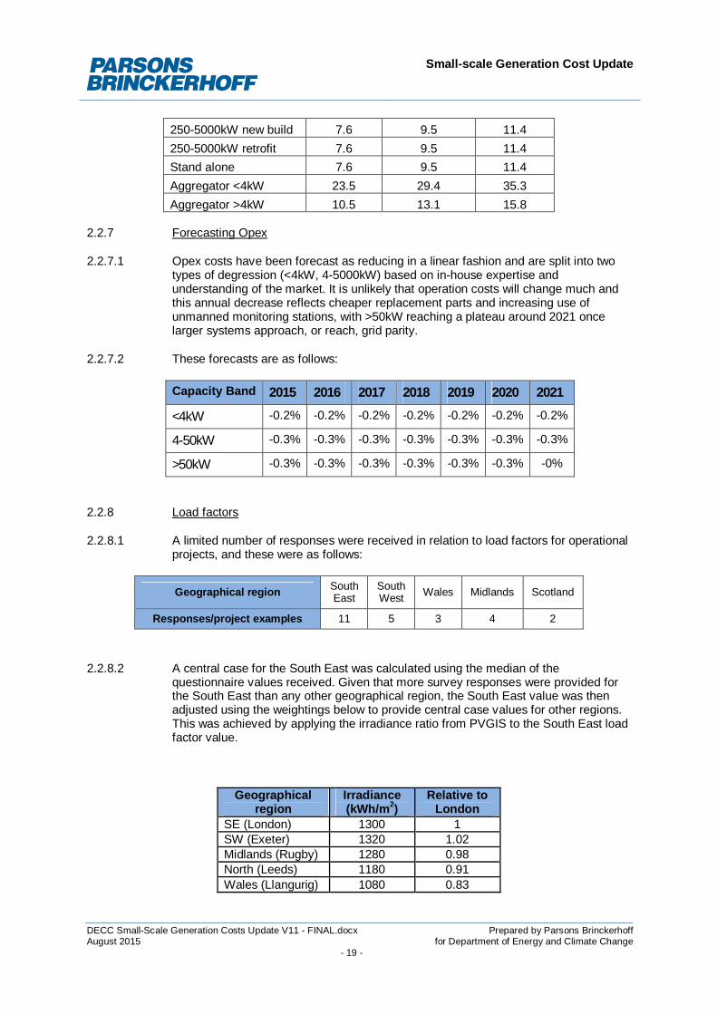
250-5000kW new build 7.6 9.5 11.4250-5000kW retrofit 7.6 9.5 11.4Stand alone 7.6 9.5 11.4Aggregator <4kW 23.5 29.4 35.3Aggregator >4kW 10.5 13.1 15.8
2.2.7 Forecasting Opex
Opex costs have been forecast as reducing in a linear fashion and are split into two2.2.7.1types of degression (<4kW, 4-5000kW) based on in-house expertise andunderstanding of the market. It is unlikely that operation costs will change much andthis annual decrease reflects cheaper replacement parts and increasing use ofunmanned monitoring stations, with >50kW reaching a plateau around 2021 oncelarger systems approach, or reach, grid parity.
These forecasts are as follows:2.2.7.2
Capacity Band 2015 2016 2017 2018 2019 2020 2021
<4kW -0.2% -0.2% -0.2% -0.2% -0.2% -0.2% -0.2%
4-50kW -0.3% -0.3% -0.3% -0.3% -0.3% -0.3% -0.3%
>50kW -0.3% -0.3% -0.3% -0.3% -0.3% -0.3% -0%
2.2.8 Load factors
A limited number of responses were received in relation to load factors for operational2.2.8.1projects, and these were as follows:
Geographical region SouthEast
SouthWest Wales Midlands Scotland
Responses/project examples 11 5 3 4 2
A central case for the South East was calculated using the median of the2.2.8.2questionnaire values received. Given that more survey responses were provided forthe South East than any other geographical region, the South East value was thenadjusted using the weightings below to provide central case values for other regions.This was achieved by applying the irradiance ratio from PVGIS to the South East loadfactor value.
Geographicalregion
Irradiance(kWh/m2)
Relative toLondon
SE (London) 1300 1SW (Exeter) 1320 1.02Midlands (Rugby) 1280 0.98North (Leeds) 1180 0.91Wales (Llangurig) 1080 0.83

Small-scale Generation Cost Update
DECC Small-Scale Generation Costs Update V11 - FINAL.docx Prepared by Parsons BrinckerhoffAugust 2015 for Department of Energy and Climate Change
- 20 -
Scotland(Glasgow) 1100 0.85
Source: PVGIS (CM-SAF)5
Low and High cases were calculated using an interquartile range of the South East2.2.8.3data set received through questionnaire responses either side of the central casevalue, which equated to ±0.6% of the central case.
Final load factor assumptions based on regional averages are as follows:2.2.8.4
RegionLoad Factor (%)
Low Case Central Case High CaseScotland 8.4% 8.9% 9.5%
Midlands 9.7% 10.3% 10.9%
South East 9.9% 10.5% 11.1%South West 10.1% 10.7% 11.3%
North 9.0% 9.6% 10.2%
Wales 8.1% 8.7% 9.3%
The load factor analysis above is based on a limited number of data points and on2.2.8.5PVGIS irradiance data which has limitations6. Both of these variables are applied at aregional level and as such, load factors at specific project locations may vary.Parsons Brinckerhoff acknowledges that load factors for PV installations could berefined further using other analytical methodologies should additional robust data besourced.
2.2.9 Expected lifetime
2.2.10 The typical lifetime for PV systems has been decreased compared to the previousmodel (from 35 to 30 years) to reflect the realistic lifetime of PV panels as witnessedwithin recent projects completed by Parsons Brinckerhoff. Note that inverterreplacement is included within the operating costs – we have considered that theinverter represents a small enough proportion of the overall capital cost for itsreplacement to be considered an operating cost.
2.2.11 Hurdle rates
The table below details the hurdle rates for solar PV calculated by Ricardo-AEA using2.2.11.1the methodology given in section 2.1.3.
5 PVGIS (Photovoltaic Geographical Information System) data available athttp://re.jrc.ec.europa.eu/pvgis/apps4/pvest.php6 Thomas Huld, Richard Müller, Attilio Gambardella, A new solar radiation database for estimating PVperformance in Europe and Africa, Solar Energy, Volume 86, Issue 6, June 2012, Pages 1803-1815.

Small-scale Generation Cost Update
DECC Small-Scale Generation Costs Update V11 - FINAL.docx Prepared by Parsons BrinckerhoffAugust 2015 for Department of Energy and Climate Change
- 21 -
Hurdle Rate (%)Low Medium High
Domestic, smallMin 0.5% 2.5% 4.5%Max 8.0% 10.0% 12.0%Avg 4.2% 6.2% 8.2%
Commercial developer,medium
Min 2.0% 4.0% 6.0%Max 9.0% 11.0% 13.0%Avg 5.0% 7.0% 9.0%
Utility, largeMin 3.0% 5.0% 7.0%Max 9.0% 11.0% 13.0%Avg 5.0% 7.0% 9.0%
The hurdle rates provided by Ricardo-AEA are comparable to the interim results2.2.11.2generated by NERA, although the range of the Ricardo-AEA data is slightly larger.
2.2.12 Technical Potential
For domestic technical potential, Parsons Brinckerhoff determined the total number of2.2.12.1households in the UK using Office for National Statistics figures7. 38% of thesebuildings were discounted due to being ‘inappropriate’ buildings such as flats (ie.apartments) or listed buildings. The average domestic building size in m2 and anassociated roof area for these buildings was calculated. It was estimated by ParsonsBrinckerhoff that 40% of appropriate buildings have a pitched roof area that pointedsouth (or south-east or south-west).
Parsons Brinckerhoff determined that the average domestic property could install a2.2.12.23.5kWp system.
For commercial technical potential, an area of 2,500 million m2 was assumed for2.2.12.3south facing commercial roofs (based on Kingspan Energy – Cutting Costs: TheEnergy Potential of UK Commercial Rooftops8). Of this 70% were assumed to bepitched roofs resulting in 1,750million m2 available. A further 30% was removed fromthe area for edging and roof obstacles, giving an availability of 1,225million m2. Thisfigure was divided by a standard module size of 1.65m2 and multiplied by the wattageof the module to get the potential output.
The remaining 30% of available roof space is assumed to be flat (750million m2). A2.2.12.4figure of 2ha per MW was used for row spacing, with a following 30% removed foredging and obstacles.
For ground-mounted technical potential, the Agriculture in the United Kingdom9 report2.2.12.5was used to give an estimate of available farm land. 10% of this was deemed to be
7 Office for National Statistics, 10 December 2013. http://www.ons.gov.uk/ons/rel/family-demography/families-and-households/2013/info-uk-households.html8 Cutting Costs: The Energy Potential of UK Commercial Rooftops, 2014. Kingspan Energy. Availableat: http://www.interfacecutthefluff.com/wp-content/uploads/2012/09/Kingspan-Energy-CUTTING-COSTS-THE-ENERGY-POTENTIAL-OF-UK-COMMERCIAL-ROOFTOPS.pdf9 Agriculture in the United Kingdom, DEFRA, 2014. Available at:https://www.gov.uk/government/uploads/system/uploads/attachment_data/file/430411/auk-2014-28may15a.pdf

Small-scale Generation Cost Update
DECC Small-Scale Generation Costs Update V11 - FINAL.docx Prepared by Parsons BrinckerhoffAugust 2015 for Department of Energy and Climate Change
- 22 -
suitable for solar PV installation (based on estimates of land topography, shading). Anassumed install of 2.5ha/MWp was used to calculate the total available capacity.
Parsons Brinckerhoff used a database from the European Joint Research Centre2.2.12.6(JRC), which uses 11 years of satellite weather data from the 1998 to mid-2010. Thisdatabase provided values for solar irradiation, temperature, wind speed andbarometric pressure for Sheffield; which subsequently provides a specific annualgeneration (896kWh/kWp) specific to the area. When the potential deployment figure(in kWp) is multiplied by this, an annual generation figure is calculated. There is anMCS requirement to provide a SAP (Standard Assessment Procedure) figure inquotations for solar PV systems. In the earlier versions of the SAP calculator therewas only one location used to determine generation, which was Sheffield. This wasused as it was a central point for the UK and will provide a most rounded figure for thestandard. .While the geometric centre of PV deployment is closer to Birmingham, thismethod has been used to maintain consistency and as the solar potential establishedconsiders the entire UK, it is a fair assumption to use this location.
The calculated technical potential for domestic properties was distributed across the2.2.12.7<4kW and aggregate <4kW bands; for commercial properties across the 4-10kW, 10-50kW and aggregate >4kW bands; and for available land across the 50-150kW, 150-250kW, 250-5000kW and standalone bands. This distribution was in line with thatgiven by CEPA in the 2012 reports. While some smaller systems may be installed asground mounted or on commercial properties, some domestic properties may alsoinstall larger systems and so the distribution balances across the capacity bands.
Capacity Band Technical Potential (GWh)Total Domestic Commercial Developer Utility
<4kW new build 223 212 11 0 0<4kW retrofit 19,201 18,241 960 0 04 - 10kW new build 241 60 181 0 04 - 10kW retrofit 23,857 5,964 17,893 0 010 - 50kW new build 1,011 0 809 101 10110 - 50kW retrofit 100,126 0 80,100 10,013 10,01350-150kW new build 240 0 191 24 2450-150kW retrofit 23,739 0 18,991 2,374 2,374150-250kW new build 279 0 253 13 13150-250kW retrofit 27,595 0 2,760 12,418 12,418250-5000kW new build 176 0 2 87 87250-5000kW retrofit 17,408 0 1,741 7,834 7,834Stand alone 129,081 0 12,908 58,086 58,086Aggregator <4kW 1,119 1,007 112 0 0Aggregator >4kW 10,658 6,395 4,263 0 0

Small-scale Generation Cost Update
DECC Small-Scale Generation Costs Update V11 - FINAL.docx Prepared by Parsons BrinckerhoffAugust 2015 for Department of Energy and Climate Change
- 23 -
2.3 Wind
2.3.1 Data Collection
Questionnaire responses were received from a wide range of consultees in relation to2.3.1.1wind projects, with 62 project-specific responses received in total, alongside aselection of additional information sources. The final assumptions presented areheavily based on questionnaire responses and the additional information receivedduring the data collection exercise, with in-company expertise drawn upon wherenecessary to fill in any data gaps. The distribution of data received is as follows:
Capacity bands <1.5kW 1.5-15kW 15-50kW 50-100kW 100-500kW 500-1500kW
1500-5000kW
Responses/projectexamples 0 2 (+2
examples) 0 11 39 10 1
For wind installations registered under the FITs scheme, information on the capital2.3.1.2and operating/maintenance costs has been updated to reflect recent price data. Otheradjustments have been made, including changes to load factors, export fractions andaverage installation size.
Details of how inputs to the model have been derived are provided below.2.3.1.3
2.3.2 De-rated Turbines
“De-rating” is the practise of limiting the electrical output of a wind turbine through2.3.2.1reducing the generator size, whereby the manufacturer can state the generatorcapacity is smaller than the maximum power it is capable of producing. The physicalsize and external appearance of the de-rated turbine is the same as that of the turbineprior to de-rating. As a result, when the turbine blades are designed for highercapacity turbines, load factors of de-rated turbines are typically higher and theoperator benefits from the higher FIT of the lower band. De-rated turbines can alsoartificially inflate the average Capex cost of turbines within the 100-500kW bandsince, for example, a larger 900kW turbine de-rated to 500kW will be likely to have ahigher capital cost than a 500kW turbine which has not been de-rated.
Within this study, Parsons Brinckerhoff has only seen evidence of 800 or 900kW2.3.2.2machines de-rated to 500kW and installed under the lower, more economicallyrewarding tariff band (100-500kW). Instances like this have been identified where thequestionnaire response has stated the turbine model installed (for example, anEnercon E44 which has a rated capacity of 900kW) and given a lower installedcapacity (generally of 500kW). Out of the 39 data points in the 100-500kW band, 20(51.3%) were derated turbines.
2.3.3 Average Installation Size
The size of a typical installation within each band has been based on the average size2.3.3.1of installations within each capacity band registered for FITs to date using dataprovided by Ofgem. Please note that the Ofgem dataset does not distinguishbetween urban and rural wind turbines in the smaller capacity bands. Theassumptions generated are as follows:

Small-scale Generation Cost Update
DECC Small-Scale Generation Costs Update V11 - FINAL.docx Prepared by Parsons BrinckerhoffAugust 2015 for Department of Energy and Climate Change
- 24 -
Capacity Band Average installation size (kW)B-M <1.5kW urban 1.65B-M <1.5kW rural 1.651.5–15kW urban 7.81.5–15kW rural 7.815–50kW urban 23.4615–50kW rural 23.4650–100kW 79.56100–500kW 379.01500–1,500kW 930.691,500-5,000kW 2911.02
2.3.4 Export Fraction
A central case was estimated for export fractions across each capacity band using the2.3.4.1average value of the data received. We have reduced the export fraction for 1.5-15kWafter reviewing the data received which largely suggests that facilities withinstallations of this type use all electricity generated on site. The assumptionsgenerated are as follows:
Capacity Band Export Fraction (%)B-M <1.5kW urban/rural 01.5–15kW urban 01.5–15kW rural 015–50kW urban 5015–50kW rural 7550–100kW 80100–500kW 85500–1,500kW 951,500-5,000kW 100
2.3.5 Capex
All Capex prices received were adjusted for inflation based on the RPI prior to the2.3.5.1methodology outlined below.
Capex prices were split as per the existing capacity bands and weightings were2.3.5.2applied to each number to adjust them based on Parsons Brinckerhoff’s confidence.The median value was found for each group. 75% either side of the median value wascalculated in order to remove outliers but these were not found. The median formedthe ‘central case’. 52% and 148% either side of the central case value forms therespective low and high cases based on one standard deviation of the dataset.
No data was received for building mounted turbines.2.3.5.3
Given the shortage of questionnaire responses and subsequent lack of confidence in2.3.5.4the <1.5kW, 1.5-15kW, 15-50kW and 1500-5000kW bands, Parsons Brinckerhoffused the above method to calculate the median values for the 100-500kW and 500-
Small-scale Generation Cost Update
DECC Small-Scale Generation Costs Update V11 - FINAL.docx Prepared by Parsons BrinckerhoffAugust 2015 for Department of Energy and Climate Change
- 25 -
1500kW bands, then used the cost change between the 2012 and the 2014assumption to guide the changes for the other bands.
The cost difference between 2012 and 2014 data for the 500-1500kW band was used2.3.5.5to adjust the 2012 data for 1500-5000kW to a 2014 value. The cost differencebetween 2012 and 2014 data for the 100-500kW band (excluding derated turbines soas not to artificially inflate the other bands) was used to adjust the 2012 data for<1.5kW, 1.5-15kW and 15-50kW to a 2014 value.
While Figure 2:2 generally shows a downward trend in Capex per kW installed with2.3.5.6increasing capacity, the data collected for 50-100kW systems lies outside of thisassumption, with a much lower Capex in £/kW than the larger turbines. While thequestionnaire did not specifically seek to understand exactly how the Capex cost wassplit between EPC, equipment and installation costs, some qualitative analysis can bedone around why this band sits apart from the other data sets.
Turbines within the 50-100kW band are generally small, monopole mounted2.3.5.7installations, with inbuilt ladders or tilt-up systems installed as standard, limiting theneed for large load-bearing concrete foundations found with larger turbine models.While smaller turbines consist of components that are reasonably simple tomanufacture and are somewhat more readily available, larger turbines including thosein the 100-500kW band utilise more specialised components available from a limitednumber of specialist manufacturers. For example, the manufacture of larger blades,tubular towers and larger generators require dedicated facilities. Smaller components(including lattice towers and smaller electrical generators) have a much wider marketavailability as they are often used for applications not related to wind energygeneration.
Questionnaire data received for the 50-100kW band, once weighted, produced an2.3.5.8anomalous result and as such, the average of the un-weighted figures was used toguide the 2014 cost assumption, which brings this assumption in line with theevidence presented above.
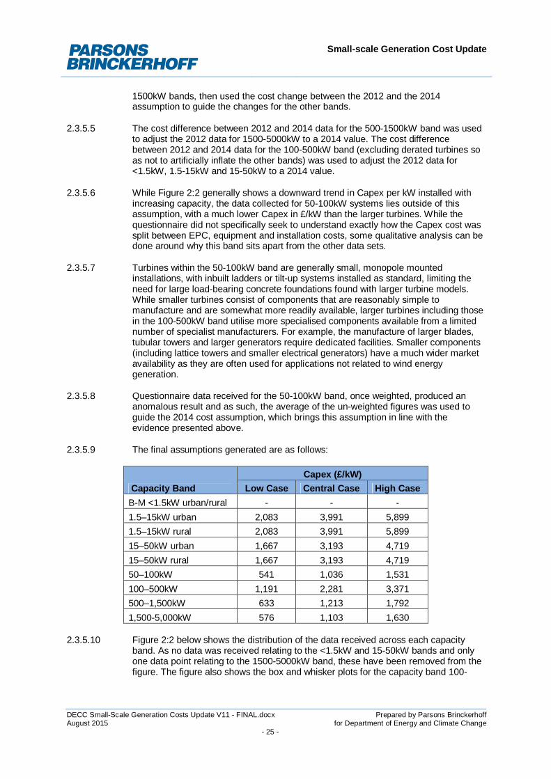
The final assumptions generated are as follows:2.3.5.9
Capacity BandCapex (£/kW)
Low Case Central Case High CaseB-M <1.5kW urban/rural - - -1.5–15kW urban 2,083 3,991 5,8991.5–15kW rural 2,083 3,991 5,89915–50kW urban 1,667 3,193 4,71915–50kW rural 1,667 3,193 4,71950–100kW 541 1,036 1,531100–500kW 1,191 2,281 3,371500–1,500kW 633 1,213 1,7921,500-5,000kW 576 1,103 1,630
Figure 2:2 below shows the distribution of the data received across each capacity2.3.5.10band. As no data was received relating to the <1.5kW and 15-50kW bands and onlyone data point relating to the 1500-5000kW band, these have been removed from thefigure. The figure also shows the box and whisker plots for the capacity band 100-
Small-scale Generation Cost Update
DECC Small-Scale Generation Costs Update V11 - FINAL.docx Prepared by Parsons BrinckerhoffAugust 2015 for Department of Energy and Climate Change
- 26 -
500kW with the de-rated turbines both included and excluded. Further discussion ofthe de-rated turbine Capex is given in Figure 2:3 and paragraphs 2.3.5.12 - 2.3.5.16below
It should also be noted that the large tariff difference between 100-500kW and 500-2.3.5.111500kW has pushed deployment in the 100-500kW band to the very edge of the bandand 92.5% of the data captured within this band was for 500kW turbines (includingde-rated models). This therefore represents a skew towards higher Capex within thisband.
Figure 2:2 Capex data per capacity band (Wind) from questionnaire responses
Please note: the data presented in Figure 2:2 does not necessarily match the data presented in the tables above.Please refer to paragraph 2.1.1.9 for an explanation.
Further analysis of the Capex of in the 100-500kW band has been carried out in2.3.5.12relation to de-rated turbines. This is illustrated in Figure 2:3 below. Columns A and Bare the same as those shown in Figure 2:2.
4 11 39 19 100
1000
2000
3000
4000
5000
6000
Cape
x(£
/kW
)
Small-scale Generation Cost Update
DECC Small-Scale Generation Costs Update V11 - FINAL.docx Prepared by Parsons BrinckerhoffAugust 2015 for Department of Energy and Climate Change
- 27 -
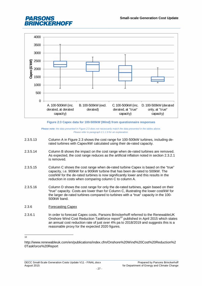
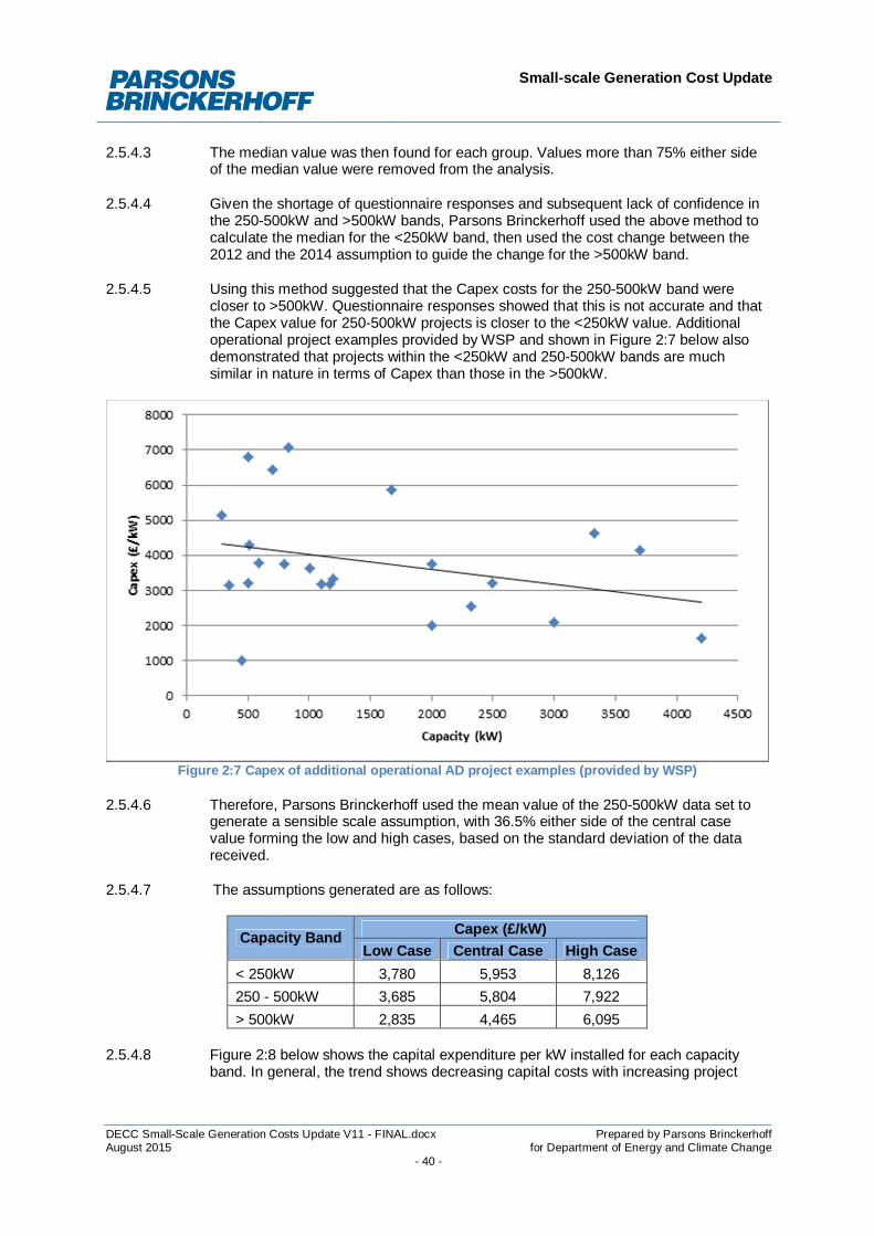
Figure 2:3 Capex data for 100-500kW (Wind) from questionnaire responses
Please note: the data presented in Figure 2:3 does not necessarily match the data presented in the tables above.Please refer to paragraph 2.1.1.9 for an explanation.
Column A in Figure 2.3 shows the cost range for 100-500kW turbines, including de-2.3.5.13rated turbines with Capex/kW calculated using their de-rated capacity.
Column B shows the impact on the cost range when de-rated turbines are removed.2.3.5.14As expected, the cost range reduces as the artificial inflation noted in section 2.3.2.1is removed.
Column C shows the cost range when de-rated turbine Capex is based on the “true”2.3.5.15capacity, i.e. 900kW for a 900kW turbine that has been de-rated to 500kW. Thecost/kW for the de-rated turbines is now significantly lower and this results in thereduction in costs when comparing column C to column A.
Column D shows the cost range for only the de-rated turbines, again based on their2.3.5.16“true” capacity. Costs are lower than for Column C, illustrating the lower cost/kW forthe larger de-rated turbines compared to turbines with a “true” capacity in the 100-500kW band.
2.3.6 Forecasting Capex
In order to forecast Capex costs, Parsons Brinckerhoff referred to the RenewableUK2.3.6.1Onshore Wind Cost Reduction Taskforce report10 published in April 2015 which statesan annual cost reduction rate of just over 4% pa to 2018/2019 and suggests this is areasonable proxy for the expected 2020 figures.
10
http://www.renewableuk.com/en/publications/index.cfm/Onshore%20Wind%20Cost%20Reduction%20Taskforce%20Report
0
500
1000
1500
2000
2500
3000
3500
4000
A. 100-500kW (inc.derated, at derated
capacity)
B. 100-500kW (excl.derated)
C. 100-500kW (inc.derated, at "true"
capacity)
D. 100-500kW (deratedonly, at "true"
capacity)
Cape
x(£
/kW
)

Small-scale Generation Cost Update
DECC Small-Scale Generation Costs Update V11 - FINAL.docx Prepared by Parsons BrinckerhoffAugust 2015 for Department of Energy and Climate Change
- 28 -
2.3.7 Opex
Opex prices were split as per the existing capacity bands and weightings were2.3.7.1applied to each number to adjust them based on Parsons Brinckerhoff’s confidence.
The median value was then found for each group. Values more than 75% either side2.3.7.2of the median value were removed from the analysis. The median (after outliers wereremoved) formed the ‘central case’. 38.6% either side of the central case value formsthe low and high cases based on the standard deviation of the data set.
As for Capex, no data relating to building-mounted turbines was received during the2.3.7.3study.
Given the shortage of questionnaire responses and subsequent lack of confidence in2.3.7.4the <1.5kW, 1.5-15kW, 15-50kW, 50-100kW, 500-1500kW and 1500-5000kW bands,Parsons Brinckerhoff used the above method to calculate the median values for the100-500kW, then used the cost change between the 2012 and the 2014 assumptionto guide the changes for the other bands. The Opex value for 100-500kW wascalculated by excluding derated turbines in this instance, so as not to artificially inflatethe Opex costs for the other bands.
The final assumptions generated are as follows:2.3.7.5
Capacity BandOpex (£/kW/year)
Low Case Central Case High CaseB-M <1.5kW urban - - -B-M <1.5kW rural - - -1.5–15kW urban 41 66 921.5–15kW rural 41 66 9215–50kW urban 28 45 6315–50kW rural 28 45 6350–100kW 25 41 56100–500kW 35 57 79500–1,500kW 17 27 381,500-5,000kW 17 27 38
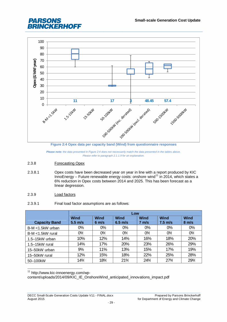
Figure 2:4 below shows the distribution of Opex data across each capacity band from2.3.7.6the survey data gathered. However, the final assumptions generated conclude thatOpex costs per kW installed per year generally decrease with capacity. While thequestionnaire did not seek to understand why this is the case, it may be that smallerturbines with a faster rotor RPM require more replacement parts over time, and thatcomponents are replaced instead of repaired. It may also be the case that manpowerrequirements are similar for larger and smaller installations, and therefore the cost perkW is higher for smaller units. Other factors may also contribute to this trend and therelative importance of each factor cannot be determined based on the data availablefrom this study.
Small-scale Generation Cost Update
DECC Small-Scale Generation Costs Update V11 - FINAL.docx Prepared by Parsons BrinckerhoffAugust 2015 for Department of Energy and Climate Change
- 29 -
Figure 2:4 Opex data per capacity band (Wind) from questionnaire responses
Please note: the data presented in Figure 2:4 does not necessarily match the data presented in the tables above.Please refer to paragraph 2.1.1.9 for an explanation.
2.3.8 Forecasting Opex
Opex costs have been decreased year on year in line with a report produced by KIC2.3.8.1InnoEnergy – Future renewable energy costs: onshore wind11 in 2014, which states a6% reduction in Opex costs between 2014 and 2025. This has been forecast as alinear degression.
2.3.9 Load factors
Final load factor assumptions are as follows:2.3.9.1
Capacity Band
LowWind5.5 m/s
Wind6 m/s
Wind6.5 m/s
Wind7 m/s
Wind7.5 m/s
Wind8 m/s
B-M <1.5kW urban 0% 0% 0% 0% 0% 0%B-M <1.5kW rural 0% 0% 0% 0% 0% 0%1.5–15kW urban 10% 12% 14% 16% 18% 20%1.5–15kW rural 14% 17% 20% 23% 26% 29%15–50kW urban 9% 11% 13% 15% 17% 19%15–50kW rural 12% 15% 18% 22% 25% 28%50–100kW 14% 18% 21% 24% 27% 29%
11 http://www.kic-innoenergy.com/wp-content/uploads/2014/09/KIC_IE_OnshoreWind_anticipated_innovations_impact.pdf
11 17 3 48.45 57.40
10
20
30
40
50
60
70
80
90
100
Ope
x(£
/kW
/yea
r)

Small-scale Generation Cost Update
DECC Small-Scale Generation Costs Update V11 - FINAL.docx Prepared by Parsons BrinckerhoffAugust 2015 for Department of Energy and Climate Change
- 30 -
100–500kW 29% 29% 35% 33% 26% 19%100–500kW(excl. derated turbines) 14% 17% 20% 24% 27% 31%
500–1,500kW 13% 17% 20% 24% 27% 31%1,500-5,000kW 15% 18% 22% 26% 29% 33%
Capacity Band
MediumWind5.5 m/s
Wind6 m/s
Wind6.5 m/s
Wind7 m/s
Wind7.5 m/s
Wind8 m/s
B-M <1.5kW urban 0% 0% 0% 0% 0% 0%B-M <1.5kW rural 0% 0% 0% 0% 0% 0%1.5–15kW urban 11% 13% 15% 17% 19% 21%1.5–15kW rural 14% 17% 21% 24% 27% 29%15–50kW urban 12% 14% 16% 18% 20% 22%15–50kW rural 13% 17% 21% 24% 28% 29%50–100kW 16% 19% 22% 25% 28% 30%100–500kW 30% 35% 43% 42% 36% 30%100–500kW(excl. derated turbines) 16% 20% 24% 28% 32% 35%
500–1,500kW 18% 22% 26% 30% 34% 38%1,500-5,000kW 21% 25% 29% 33% 37% 41%
Capacity Band
HighWind5.5 m/s
Wind6 m/s
Wind6.5 m/s
Wind7 m/s
Wind7.5 m/s
Wind8 m/s
B-M <1.5kW urban 0% 0% 0% 0% 0% 0%B-M <1.5kW rural 0% 0% 0% 0% 0% 0%1.5–15kW urban 15% 17% 19% 21% 23% 25%1.5–15kW rural 22% 24% 26% 28% 29% 29%15–50kW urban 18% 20% 22% 24% 26% 28%15–50kW rural 22% 24% 26% 28% 29% 32%50–100kW 17% 21% 24% 27% 29% 31%100–500kW 32% 37% 58% 50% 42% 34%100–500kW(excl. derated turbines) 19% 23% 27% 30% 34% 37%
500–1,500kW 20% 24% 29% 33% 37% 40%1,500-5,000kW 23% 28% 32% 37% 41% 44%
Parsons Brinckerhoff reviewed the original 2012 estimates for each band with high,2.3.9.2central and low scenarios and recommends continuing to use them. These resultswere cross-checked with the results from the questionnaires and also compared tothe current estimates with several other Parsons Brinckerhoff wind farms indevelopment or in construction where bankable energy assessment were provided.
In the period 2012-2014, the number of manufacturers that significantly improved their2.3.9.3model performances (efficiency, overall electricity produced) is limited. Mostmanufacturers released different or bigger models to cope with the uptake in the off-shore market. Capex and production costs have decreased to improve their

Small-scale Generation Cost Update
DECC Small-Scale Generation Costs Update V11 - FINAL.docx Prepared by Parsons BrinckerhoffAugust 2015 for Department of Energy and Climate Change
- 31 -
competitiveness; however, Parsons Brinckerhoff experience suggests that nosignificant increase of performance was registered in this period.
However, the practise of derating turbines has meant that in the 100-500kW band2.3.9.4load factors received throughout the data collection exercise were generally higherthan previously specified. As such, load factors in the central and high case bandshave been updated to reflect the higher load factors seen, with the median value ofthe capacity band for each average wind speed (where questionnaire data wasreceived) forming the central case. Where questionnaire data did not provide loadfactor data for a specific wind speed, the mid-point of the data either side of themissing point was used to generate a central case. For all other bands, ParsonsBrinckerhoff does not believe that on-shore wind technology has moved forwardenough to justify a change in the existing numbers.
The history of wind turbines is that of steadily increasing performance as the2.3.9.5technology is improved and blade aerodynamic efficiency is optimised. There istherefore the potential that in the future, new wind turbine installations will make useof improved technology to produce higher load factors. It is also conceivable that insome instances, existing wind turbine installations may retrofit (eg. componentreplacement) or repower using improved technology to yield higher loadfactors. Since future technology improvements are by their very nature unpredictable,developments in this area might materially alter these conclusions and should bemonitored.
2.3.10 Expected lifetime
This has been retained at 20 years in line with the previous report. It is not considered2.3.10.1that wind technology has changed so significantly in the last two years that it wouldaffect the operational lifetime of the plant.
2.3.11 Hurdle rates
The table below displays the hurdle rates for wind that were suggested by Ricardo-2.3.11.1AEA using the methodology described in section 2.1.3.
Hurdle Rate (%)Low Medium High
Domestic, smallMin 1.0% 3.0% 5.0%Max 9.0% 11.0% 13.0%Avg 4.5% 6.5% 8.5%
Commercial developer, mediumMin 3.0% 5.0% 7.0%Max 10.0% 12.0% 14.0%Avg 6.3% 8.3% 10.3%
Utility, large
Min 3.0% 5.0% 7.0%Max 12.0% 14.0% 16.0%Avg 6.3% 8.3% 10.3%
The figures provided by Ricardo-AEA were compared to the interim results generated2.3.11.2by NERA and are comparable with very similar central case values.

Small-scale Generation Cost Update
DECC Small-Scale Generation Costs Update V11 - FINAL.docx Prepared by Parsons BrinckerhoffAugust 2015 for Department of Energy and Climate Change
- 32 -
2.3.12 Technical Potential
CEPA predicted technical potential for wind within their cost of generation update2.3.12.1published in 2012. The values used were taken from the DECC model published priorto the 2012 update, after a check to ensure that they were still considered reasonable.
Parsons Brinckerhoff has retained these values within this update. There is shortage2.3.12.2of revised information since 2012 and, because wind is considered a maturetechnology and the available land area in the UK will not have changed significantlysince 2012, Parsons Brinckerhoff believes these figures and the distribution ofpotential across the bands are accurate. We have updated the overall technicalpotential based on the updated load factor assumptions (central case) given withinthis report.
Capacity Band Technical Potential (GWh)Total Domestic Commercial Developer Utility
B-M <1.5kW urban 0 0 0 0 0
B-M <1.5kW rural 0 0 0 0 0
1.5–15kW urban 0 0 0 0 0
1.5–15kW rural 1,610 644 966 0 0
15–50kW urban 0 0 0 0 0
15–50kW rural 1,352 135 1,216 0 0
50–100kW 580 0 580 0 0
100–500kW 3,694 0 0 2,955 739
500–1,500kW 814 0 0 651 163
1,500-5,000kW 3,917 0 0 1,958 1,958
Small-scale Generation Cost Update
DECC Small-Scale Generation Costs Update V11 - FINAL.docx Prepared by Parsons BrinckerhoffAugust 2015 for Department of Energy and Climate Change
- 33 -
2.4 Hydro
2.4.1 Data Collection
Questionnaire responses were received from a wide range of consultees in relation to2.4.1.1hydro projects, with 54 project-specific responses received in total, alongside aselection of additional information sources. The final assumptions presented areheavily based on questionnaire responses and the additional information receivedduring the data collection exercise, with in-company expertise drawn upon wherenecessary to fill in any data gaps. The distribution of data received is as follows:
Capacity bands <15kW 15-50kW 50-100kW 100-500kW 500-
1000kW1000-
2000kW2000-
5000kWResponses/projectexamples 9 9 6 15 6 8 0
For hydro installations registered under the FITs scheme, information on the capital2.4.1.2and operating/maintenance costs has been updated to reflect recent price data. Otheradjustments have been made, including changes to load factors, export fractions andaverage installation size.
Details of how inputs to the model have been derived are provided below.2.4.1.3
2.4.2 Average Installation Size
The size of a typical installation within each band has been based on the average size2.4.2.1of installations within each capacity band registered for FITs to date using dataprovided by Ofgem. The assumptions are as follows:
Capacity Band Average installation size (kW)<15kW 8.415–50kW 33.3650–100kW 85.1100–500kW 345.48500–1,000kW 754.191,000–2,000kW 1518.42,000–5,000kW 2253
2.4.3 Export Fraction
A central case was estimated for export fractions across each capacity band using the2.4.3.1average value of the data received.
Capacity Band Export Fraction (%)<15kW 2015–50kW 7550–100kW 75100–500kW 88500–1,000kW 991,000–2,000kW 99

Small-scale Generation Cost Update
DECC Small-Scale Generation Costs Update V11 - FINAL.docx Prepared by Parsons BrinckerhoffAugust 2015 for Department of Energy and Climate Change
- 34 -
Capacity Band Export Fraction (%)2,000–5,000kW 99
2.4.4 Capex
All Capex prices received were adjusted for inflation based on the RPI prior to the2.4.4.1methodology outlined below.
Capex prices were split as per the existing capacity bands and weightings were2.4.4.2applied to each number to adjust them based on Parsons Brinckerhoff’s confidence.
The median value was then found for each group. Values more than 75% either side2.4.4.3of the median value were removed from the analysis. The median formed the ‘centralcase’. 48% either side of the central case value forms the low and high cases basedon the standard deviation of the data points gathered.
Given the shortage of questionnaire responses and subsequent lack of confidence in2.4.4.4the 50-100kW, 500-1000kW, 1000-2000kW and 2000-5000kW bands, ParsonsBrinckerhoff used the above method to calculate the median values for the 15-50kWand 100-500kW bands, then used the average cost change between the 2012 andthe 2014 assumption to guide the changes for the other bands. The <15kWassumption was generated based on survey results alone.
The assumptions generated are as follows:2.4.4.5
Capacity Band Capex (£/kW)Low Case Central Case High Case
<15kW 1,873 3,603 5,33215–50kW 2,900 5,577 8,25450–100kW 2,682 5,158 7,635100–500kW 2,158 4,150 6,143500–1,000kW 1,694 3,258 4,8221,000–2,000kW 1,331 2,560 3,7892,000–5,000kW 1,089 2,095 3,100
Figure 2:5 below shows how the distribution of the data varies with each capacity2.4.4.6size. It is evident from the data presented in Figure 2:5 that there is not a clear trendin Capex for hydro schemes across the capacity bands; Parsons Brinckerhoff’s viewis that the likely reason for an absence of a trend is because each hydro project isunique in its construction and design requirements. The distribution of data withineach capacity band is very large, even when outliers have been removed from thedata sets. Note that due to a shortage of data collected, the box and whisker plot forCapex of 2000-5000kW projects has not been included.
The data suggests that determining an average Capex value for hydro projects across2.4.4.7any of the capacity bands is difficult given the varying levels of design and buildcomplexity. While Parsons Brinckerhoff has more confidence in the <15kW, 15-50kW,and 100-500kW than the other bands given the larger quantities of questionnaire datareceived, the data are still largely spread, both across the individual bands and acrossthe entire data set.

Small-scale Generation Cost Update
DECC Small-Scale Generation Costs Update V11 - FINAL.docx Prepared by Parsons BrinckerhoffAugust 2015 for Department of Energy and Climate Change
- 35 -
Figure 2:5 Capex data per capacity band (Hydro) from questionnaire responses
Please note: the data presented in Figure 2:5 does not necessarily match the data presented in the tables above.Please refer to paragraph 2.1.1.9 for an explanation.
2.4.5 Forecasting Capex
Parsons Brinckerhoff referred to the IRENA Renewable Power Generation Costs in2.4.5.12014 report which confirms that hydro is a mature technology with limited costreduction potential. Parsons Brinckerhoff has therefore assumed a 0% per year linearcost reduction up to 2021; this figure is used as a balance between small changes inmanufacturing methods which may decrease hydro Capex costs and rising installationcosts across more complex sites.
2.4.6 Opex
Opex prices were split as per the existing capacity bands and weightings were2.4.6.1applied to each number to adjust them based on Parsons Brinckerhoff’s confidence.
The median value was then found for each group. Values more than 75% either side2.4.6.2of the median value were removed from the analysis. The median formed the ‘centralcase’. 94.2% either side of the central case value forms the low and high cases.
Given the shortage of questionnaire responses relating to Opex costs, Parsons2.4.6.3Brinckerhoff only had real confidence in the 100-500kW and 1000-2000kW bands,Parsons Brinckerhoff used the above method to calculate the median values for thesebands, then used the cost change between the 2012 and the 2014 assumption toguide the changes for the other bands.
The cost difference between 2012 and 2014 data for the 100-500kW band was used2.4.6.4to adjust the 2012 data for <15kW, 15-50kW and 50-100kW bands to their 2014value. The cost difference between 2012 and 2014 data for the 1000-2000kW bandwas used to adjust the 2012 data for 2000-5000kW to a 2014 value. The average of
5 7 5 10 6 80
2000
4000
6000
8000
10000
12000
Cape
x(£
/kW
)

Small-scale Generation Cost Update
DECC Small-Scale Generation Costs Update V11 - FINAL.docx Prepared by Parsons BrinckerhoffAugust 2015 for Department of Energy and Climate Change
- 36 -
the two costs differences was used to calculate the cost change for the 500-1000kWband.
The final assumptions generated are as follows:2.4.6.5
Capacity BandOpex (£/kW/year)
Low Case Central Case High Case<15kW 2 42 8215–50kW 4 67 13050–100kW 5 93 181100–500kW 3 51 99500–1,000kW 1 21 411,000–2,000kW 1 12 232,000–5,000kW 0 5 10
Figure 2:6 shows how the distribution of the data varies with each capacity size. The2.4.6.6trend largely shows decreasing annual operational costs per kW with increasingproject capacity.
Figure 2:6 Opex data per capacity band (Hydro) from questionnaire responses
Please note: the data presented in Figure 2:6 does not necessarily match the data presented in the tables above.Please refer to paragraph 2.1.1.9 for an explanation.
6 6 3 10 6
7
0
50
100
150
200
250
Ope
x(£
/kW
/yea
r)

Small-scale Generation Cost Update
DECC Small-Scale Generation Costs Update V11 - FINAL.docx Prepared by Parsons BrinckerhoffAugust 2015 for Department of Energy and Climate Change
- 37 -
2.4.7 Forecasting Opex
Opex costs have not been changed while predicting forward as it is not envisaged2.4.7.1that methods around operating and maintaining hydro generating plant will change.This is in line with the figures predicted during the 2012 report.
2.4.8 Load factors
The load factors presented below have been increased in comparison to 20122.4.8.1assumptions.
The central case load factor assumption was generated by calculating the median of2.4.8.2the questionnaire data collected. One standard deviation of this data either sideprovides the low and high cases.
Load Factor (%)Low Central High27% 40% 53%
Much higher load factors were witnessed in the questionnaire responses, particularly2.4.8.3in relation to turbines <15kW, where operational load factors as high as 70% wereseen, and anticipated load factors of 85% were stated.
Parsons Brinckerhoff also recognise that turbines are sometimes undersized for the2.4.8.4water course they are installed in, possibly as a result of grid availability in more ruralareas, which leads to distorted, higher load factors. While these load factors wereincluded in the calculation of the cases presented above, the high case was notskewed to include these higher load factor instances.
2.4.9 Expected lifetime
Responses to the survey state that the useful project life (economic life) for hydro2.4.9.1installations is 25–75 years with an average value of 35 years. While the civilstructure and the turbine can exist for huge lengths of time, the electrical and Balanceof Plant components may need replacing after 15-20 years and as such, 35 years hasbeen assumed as a reasonable lifetime. This has been increased in comparison tothe 2012 report, which stated a 25 year lifetime.
2.4.10 Hurdle rates
The table below displays the hurdle rates for hydro that were suggested by Ricardo-2.4.10.1AEA using the methodology as described in section 2.1.3.
Hurdle Rate (%)Low Medium High
Domestic, smallMin 1.00% 3.00% 5.00%Max 9.00% 11.00% 13.00%Avg 4.50% 6.50% 8.50%
Commercial developer,medium
Min 7.00% 9.00% 11.00%Max 13.00% 15.00% 17.00%Avg 9.00% 11.00% 13.00%

Small-scale Generation Cost Update
DECC Small-Scale Generation Costs Update V11 - FINAL.docx Prepared by Parsons BrinckerhoffAugust 2015 for Department of Energy and Climate Change
- 38 -
Utility, largeMin 5.00% 7.00% 9.00%Max 13.00% 15.00% 17.00%Avg 6.50% 8.50% 10.50%
The assumptions provided by Ricardo-AEA were compared to the interim results2.4.10.2generated by NERA and were found to be very similar, although the ranges aredifferent particularly at the high end.
2.4.11 Technical Potential
CEPA predicted technical potential for hydro within their cost of generation update2.4.11.1published in 2012. These values were derived from the 2010 Environment Agencyreport ‘Mapping Hydropower Opportunities and Sensitivities in England and Wales’12
and the 2009 Element Energy/Poyry report on the Feed-In Tariff Design.
As hydro is considered a mature technology and the number of rivers/water bodies in2.4.11.2the UK has not changed since 2012, Parsons Brinckerhoff believes the powerpotential figures given in the Environment Agency report are still accurate. This reportwas used to guide the 2014 technical potential assumptions.
The power potential figures given within the Environment Agency report were split into2.4.11.3the current FIT capacity bands shown below and multiplied by the central case loadfactor given in 2.4.8 above to determine a technical potential figure for each capacityband. The distribution of this potential generation across domestic, commercial,developer and utility-scale projects within each band was retained as for the 2012assumptions.
Capacity Band Technical Potential (GWh)Total Domestic Commercial Developer Utility
<15kW 305 229 76 0 015–50kW 553 24 144 385 050–100kW 441 0 44 353 44100–500kW 1,365 0 0 683 682500–1,000kW 618 0 0 309 3091,000–2,000kW 769 0 0 384 3842,000–5,000kW 902 0 0 451 451
12 Mapping Hydropower Opportunities and Sensitivities in England and Wales – Technical Report,Environment Agency, February 2010. Available at: http://www.climate-em.org.uk/images/uploads/GEHO0310BRZH-E-E_technical_report.pdf

Small-scale Generation Cost Update
DECC Small-Scale Generation Costs Update V11 - FINAL.docx Prepared by Parsons BrinckerhoffAugust 2015 for Department of Energy and Climate Change
- 39 -
2.5 Anaerobic Digestion
2.5.1 Data Collection
A total of 21 project-specific questionnaire responses were received for AD projects,2.5.1.1alongside a selection of additional information sources and specialist input providedby WSP. The final assumptions presented are heavily based on questionnaireresponses and the additional information received during the data collection exercise,with in-company expertise drawn upon where necessary to fill in any data gaps. Thedistribution of data received is as follows:
Capacity bands <250kW 250-500kW >500kW
Responses/projectexamples
4 (+17Capex/Opex
data only)
12 (5 withno costdata)
5
For AD installations registered under the FITs scheme, information on the capital and2.5.1.2operating/maintenance costs has been updated to reflect recent price data. Otheradjustments have been made, including changes to load factors, export fractions andaverage installation size.
Details of how inputs to the model have been derived are provided below.2.5.1.3
2.5.2 Average Installation Size
The size of a typical installation within each band has been based on the average size2.5.2.1of installations within each capacity band registered for FITs to date using dataprovided by Ofgem. The assumptions are as follows:
Capacity Band Average installation size (kW)AD < 250kW 155.26AD 250 - 500kW 479AD > 500kW 1414.81
2.5.3 Export Fraction
A central case was estimated for export fractions across each capacity band using the2.5.3.1average value of the data received.
Capacity Band Export Fraction (%)AD < 250kW 75AD 250 - 500kW 90AD > 500kW 95
2.5.4 Capex
All Capex prices received were adjusted for inflation based on the RPI prior to the2.5.4.1methodology outlined below.
Capex prices were split as per the existing capacity bands and weightings were2.5.4.2applied to each number to adjust them based on Parsons Brinckerhoff’s confidence.
Small-scale Generation Cost Update
DECC Small-Scale Generation Costs Update V11 - FINAL.docx Prepared by Parsons BrinckerhoffAugust 2015 for Department of Energy and Climate Change
- 40 -
The median value was then found for each group. Values more than 75% either side2.5.4.3of the median value were removed from the analysis.
Given the shortage of questionnaire responses and subsequent lack of confidence in2.5.4.4the 250-500kW and >500kW bands, Parsons Brinckerhoff used the above method tocalculate the median for the <250kW band, then used the cost change between the2012 and the 2014 assumption to guide the change for the >500kW band.
Using this method suggested that the Capex costs for the 250-500kW band were2.5.4.5closer to >500kW. Questionnaire responses showed that this is not accurate and thatthe Capex value for 250-500kW projects is closer to the <250kW value. Additionaloperational project examples provided by WSP and shown in Figure 2:7 below alsodemonstrated that projects within the <250kW and 250-500kW bands are muchsimilar in nature in terms of Capex than those in the >500kW.
Figure 2:7 Capex of additional operational AD project examples (provided by WSP)
Therefore, Parsons Brinckerhoff used the mean value of the 250-500kW data set to2.5.4.6generate a sensible scale assumption, with 36.5% either side of the central casevalue forming the low and high cases, based on the standard deviation of the datareceived.
The assumptions generated are as follows:2.5.4.7
Capacity Band Capex (£/kW)Low Case Central Case High Case
< 250kW 3,780 5,953 8,126250 - 500kW 3,685 5,804 7,922> 500kW 2,835 4,465 6,095
Figure 2:8 below shows the capital expenditure per kW installed for each capacity2.5.4.8band. In general, the trend shows decreasing capital costs with increasing project

Small-scale Generation Cost Update
DECC Small-Scale Generation Costs Update V11 - FINAL.docx Prepared by Parsons BrinckerhoffAugust 2015 for Department of Energy and Climate Change
- 41 -
size, although the variation around the smaller plants is large, possibly due to thedifferent types of feedstock processed and therefore different plant configurations.
Figure 2:8 Capex data per capacity band (AD) from questionnaire responses
Please note: the data presented in Figure 2:8 does not necessarily match the data presented in the tables above.Please refer to paragraph 2.1.1.9 for an explanation.
2.5.5 Forecasting Capex
No formal reports were identified that provided evidenced figures for a forecasted2.5.5.1change in Capex costs relating to AD. Parsons Brinckerhoff has employed the use oftheir in-house Technical Leadership Team to determine suitable assumptions for thefuture costs of AD.
Capex costs have been forecast in line with predictions assumed under the previous2.5.5.2work completed by CEPA. This is based on the assumption that the technology willcontinue to mature slightly, allowing for some further small reductions in cost, largelythrough reduction in project risks. Capex costs have been forecasted at decreasing1% annually until 2021, from which point onwards they will decrease by 0.5% peryear.
2.5.6 Opex
Opex prices were split as per the existing capacity bands and weightings were2.5.6.1applied to each number to adjust them based on Parsons Brinckerhoff’s confidence.
The median value was then found for each group. Values more than 75% either side2.5.6.2of the median value were removed from the analysis. The median formed the ‘centralcase’. 64.7% either side of the central case value forms the low and high cases,based on the standard deviation of the data received.
0
2000
4000
6000
8000
10000
12000
<250kW 250-500kW >500kW
Cape
x(£
/kW
)

Small-scale Generation Cost Update
DECC Small-Scale Generation Costs Update V11 - FINAL.docx Prepared by Parsons BrinckerhoffAugust 2015 for Department of Energy and Climate Change
- 42 -
Given the shortage of questionnaire responses and subsequent lack of confidence in2.5.6.3the 250-500kW and >500kW bands, Parsons Brinckerhoff used the above method tocalculate the median for the <250kW band, then used the cost change between the2012 and the 2014 assumption to guide the changes for the other two bands.
The assumptions generated are as follows:2.5.6.4
Capacity BandOpex (£/kW/year)
Low Case CentralCase High Case
< 250kW 268 759 1,250250 - 500kW 228 645 1,062> 500kW 240 679 1,118
Figure 2:9 below shows the annual operating costs per kW across the different2.5.6.5capacity bands. The trend largely shows that with increasing project size, annualoperating costs per kW decrease. Uncertainty around the smaller projects (<250kW)is large as methods of operation and maintenance vary significantly, from dedicatedOperation & Maintenance contracts to owner-made repairs.
Figure 2:9 Opex data per capacity band (AD) from questionnaire responses
Please note: the data presented in Figure 2:9 does not necessarily match the data presented in the tables above.Please refer to paragraph 2.1.1.9 for an explanation.
Please refer to paragraph 3.3 for further analysis on feedstock types and costs, and2.5.6.6paragraph 3.5 for discussion around digestate disposal costs. The Opex costs quotedabove are exclusive of feedstock and digestate disposal costs.
0
200
400
600
800
1000
1200
1400
<250kW 250-500kW >500kW
Ope
x(£
/kW
/yr)

Small-scale Generation Cost Update
DECC Small-Scale Generation Costs Update V11 - FINAL.docx Prepared by Parsons BrinckerhoffAugust 2015 for Department of Energy and Climate Change
- 43 -
2.5.7 Forecasting Opex
No formal reports were identified that provided evidenced figures for a forecasted2.5.7.1change in Capex costs relating to AD. Parsons Brinckerhoff has employed the use oftheir in-house Technical Leadership Team to determine suitable assumptions for thefuture costs of AD.
Future Opex costs are assumed to be flat, as in the previous assumptions. This2.5.7.2assumption was confirmed by the Parsons Brinckerhoff Technical Leadership Team.Operations and maintenance varies wildly across the capacity bands, with smallerinstallations maintained by the farmers who own them, and larger installations with adedicated Operation & Maintenance contract reflective of the project lifetime.
2.5.8 Load factors
The load factor is defined as the actual output over a year compared to the output2.5.8.1from the installed capacity running continually throughout the year.
Load factors and efficiencies for AD across all capacity bands are higher than in the2.5.8.2previous model, based on collected data on actual load factors achieved in practiceby UK installations.
Capacity Band Electricity Load Factor (%)Low Medium High
AD < 250kW 63% 65% 67%AD 250 - 500kW 68% 70% 72%AD > 500kW 77% 80% 83%
Questionnaire data received suggested that load factors were higher than the2.5.8.3assumptions given in the table above, at around 90-94% across all capacity bands;however, further review from WSP confirmed that these were likely to be load factorswhich excluded availability, and that once availability (be it seasonal or as a result offeedstock availability or maintenance) was taken into account, load factors would bemuch closer to those quoted in the table above.
These load factors in line with those quoted by the Green Investment Bank13 which2.5.8.4state an ‘operational performance for agricultural facilities in 2014 [of] 71 per cent…[with a] corresponding figure [of] 72 per cent for source segregated food facilities’.
2.5.9 Expected lifetime
This has been retained at 20 years in line with the previous report. It is not considered2.5.9.1that AD technology has changed so significantly in the last two years that it wouldaffect the operational lifetime of the plant.
2.5.10 Hurdle rates
13 The UK Anaerobic Digestion Market, Green Investment Bank, March 2015. Available athttp://www.greeninvestmentbank.com/media/44758/gib-anaerobic-digestion-report-march-2015-final.pdf

Small-scale Generation Cost Update
DECC Small-Scale Generation Costs Update V11 - FINAL.docx Prepared by Parsons BrinckerhoffAugust 2015 for Department of Energy and Climate Change
- 44 -
The table below displays the hurdle rates for AD that were suggested by Ricardo-AEA2.5.10.1using the methodology as described in section 2.1.3.
Hurdle Rate (%)Low Medium High
Commercial developer,medium
Min 7.0% 9.0% 11.0%Max 12.0% 14.0% 16.0%Avg 11.0% 13.0% 15.0%
Utility, largeMin 6.0% 8.0% 10.0%Max 11.0% 13.0% 15.0%Avg 10.0% 12.0% 14.0%
The hurdle rates provided by Ricardo-AEA appear to be reasonably comparable to2.5.10.2those calculated by NERA. The central case value is slightly higher for Ricardo-AEAhowever the ranges are similar overall.
2.5.11 Technical Potential
CEPA predicted technical potential for AD within their cost of generation update2.5.11.1published in 2012. This potential was based on DEFRA’s 2011 Anaerobic DigestionStrategy and Action Plan, taking into account the expectation that waste reductionmeasures will reduce potential over time. Parsons Brinckerhoff has used these valuesas it is our belief that they still reflect the current technical potential within the UK, buthave used the 2014 load factor assumptions (central case) given within this report toupdate the total technical potential.
The technical potential assumptions are as follows:2.5.11.2
Capacity BandTechnical Potential (GWh)
Total Domestic Commercial Developer UtilityAD < 250kW 867 0 433 433 0AD 250 - 500kW 862 0 172 689 0AD > 500kW 1,600 0 0 1,600 0

Small-scale Generation Cost Update
DECC Small-Scale Generation Costs Update V11 - FINAL.docx Prepared by Parsons BrinckerhoffAugust 2015 for Department of Energy and Climate Change
- 45 -
2.6 Micro CHP
2.6.1 Average Installation Size
The size of a typical installation for mCHP has been based on the average size of2.6.1.1installation registered for FITs to date using data provided by Ofgem.
Capacity Band Average Installation Size (kW)<2kW 1.04
2.6.2 Export Fraction
The value calculated for export fraction was based on heat demand modelling results2.6.2.1from the Baxi Ecogen (Stirling engine) system. This range varies from 14-26% and isbased on the understanding that the UK average daily electricity demand is lower inthe morning and higher in the evening, whereas heat demand is generally highest inthe morning through the winter. As such, a reasonable proportion of generatedelectricity could be exported to the grid, but this would vary according to householdpower consumption.
Capacity Band Export Fraction (%)
<2kW 20
2.6.3 Capex
Due to a lack of survey responses, Capex data was based on installation prices for2.6.3.1the only mCHP systems seemingly available for installation in the United Kingdom –the Baxi Ecogen (Stirling engine).
An average value was taken from the two systems available (natural gas and LPG2.6.3.2models) to give a Capex price. The low case was calculated from the sale price of thecheaper system (£7,615) with a £1,800 installation cost, and the high case calculatedfrom the full price system cost of the more expensive system (£8,642), with a £1,800installation cost.
CapacityBand
Capex (£/kW)Low Central High
<2kW 9,415 9,929 10,442
2.6.4 Opex
Due to a lack of survey responses, Opex data was based on estimates of typical2.6.4.1annual boiler servicing costs and through the modelling of heat demand based on theBaxi Ecogen (Stirling engine) system.
CapacityBand
Capex (£/kW)Low Case Central Case High Case
<2kW 50 63 75

Small-scale Generation Cost Update
DECC Small-Scale Generation Costs Update V11 - FINAL.docx Prepared by Parsons BrinckerhoffAugust 2015 for Department of Energy and Climate Change
- 46 -
2.6.5 Load factors
The assumption for load factor was calculated based on estimates for annual2.6.5.1domestic heat load requirement profiling previously completed in house by ParsonsBrinckerhoff and on heat demand modelling completed for the Baxi Ecogen (Stirlingengine) system. Load factors are expected to be in the range of 14-38%.
Capacity Band Load Factor (%)
<2kW 26
2.6.6 Expected lifetime
A lifetime of 10 years has been estimated based on publically available information2.6.6.1relating to mCHP systems and lifetimes guaranteed by manufacturers.
2.6.7 Hurdle rates
Hurdle rates for micro-CHP were not evaluated by Ricardo-AEA or NERA.2.6.7.1

Small-scale Generation Cost Update
DECC Small-Scale Generation Costs Update V11 - FINAL.docx Prepared by Parsons BrinckerhoffAugust 2015 for Department of Energy and Climate Change
- 47 -
3 REVIEW OF OTHER INPUTS
The following section outlines further work completed in relation to a number of key3.1.1.1questions raised by DECC and other stakeholders throughout the data collectionexercise.
3.2 Grid Connection Costs
Grid connection costs can form a large part of a project’s capital outlay. Parsons3.2.1.1Brinckerhoff has collected project specific grid connection details as part of thisexercise in a bid to understand how connection costs, types and project distance fromthe point of grid connection affects project feasibility. Grid connection costs wererequested as a separate item within the project pricing details sought by thequestionnaires.
The following graphs contain data from real wind, hydro and AD project examples to3.2.1.2show how the cost of grid connection varies with distance from the point of connection(PoC) and type of connection. Figure 3:1 shows all data points received, while Figure3:2 shows those less than 2km from the point of connection.
Figure 3:1 The variation of grid connection costs with distance from the PoC
£0
£200,000
£400,000
£600,000
£800,000
£1,000,000
£1,200,000
£1,400,000
£1,600,000
£1,800,000
0 5 10 15
Grid
conn
ectio
nco
st(£
)
Distance from grid connection (km)
Underground
Overhead
Combination
Figure 3:2

Small-scale Generation Cost Update
DECC Small-Scale Generation Costs Update V11 - FINAL.docx Prepared by Parsons BrinckerhoffAugust 2015 for Department of Energy and Climate Change
- 48 -
Figure 3:2 The variation of grid connection costs with distance from the PoC
The figures above suggest that there is no correlation between grid connection cost3.2.1.3and the distance to PoC operated by the local district network operator, regardless ofconnection type.
Naturally, the greater the distance from the generating facility to the PoC, the higher3.2.1.4the costs of transmission lines and associated work and this cost alone would displaya correlation between cost and distance. However, grid connection costs can belargely dependent on the PoC itself as additional costs are incurred when upgradeshave to be made at the substation to accommodate the incoming energy from theconnected generating facility. These upgrades will vary hugely depending on the PoCand different capacity connections will force different upgrades. As a result of this, thegraph above shows no correlation and connections costs are unable to be predicted.
The connection process applies to all technologies eligible under the FIT and due to3.2.1.5the huge variability in general connection requirements, it is envisaged that there willbe no definitive correlation between cost, technology, capacity and distance.
It is worth noting that smaller projects (typically <50kW) can often be connected to3.2.1.6localised distribution boards (such as in domestic/commercial properties) in place ofbeing connected to a substation, which therefore incurs no grid connection cost.
£0
£50,000
£100,000
£150,000
£200,000
£250,000
£300,000
£350,000
£400,000
0 0.5 1 1.5 2
Grid
conn
ectio
nco
st(£
)
Distance from grid connection (km)
Underground
Overhead
Combination

Small-scale Generation Cost Update
DECC Small-Scale Generation Costs Update V11 - FINAL.docx Prepared by Parsons BrinckerhoffAugust 2015 for Department of Energy and Climate Change
- 49 -
Figure 3:3 Grid connection costs against capacity for all questionnaire responses received
Figure 3:3 above shows how grid connection costs (in £/kW) vary with project3.2.1.7capacity, using data on grid connection costs obtained from 131 questionnaireresponses. There is a weak negative correlation between the two variables, althoughthe number of data points at 500kW demonstrates just how much grid connectioncosts can vary from project to project.
Parsons Brinckerhoff approximated grid connection costs for the capacity bands3.2.1.8across this study, by drawing a linear trendline through the data and using the mid-point of the following capacity bands. The following table outlines the suggestedcentral case for grid connection costs across the small-scale renewable technologyrange:
Capacity Band Grid Connection Cost (Central case) (£/kW)0–15kW £385.6015–50kW £384.6250–100kW £382.97100–500kW £374.19500–1,500kW £346.891,500-5,000kW £259.14
3.3 Feedstock Types, Costs and Gate Fees – Anaerobic Digestion
The questionnaires issued to industry for anaerobic digestion projects sought to3.3.1.1understand the types of feedstock used across each capacity bands and theassociated costs and supply chains for these feedstock types. Opex costs quotedwithin this report are exclusive of feedstock costs and gate fees.
0
200
400
600
800
1000
1200
1400
1600
1800
2000
0 500 1000 1500 2000 2500 3000 3500 4000 4500 5000
Grid
Conn
ectio
nCo
st(£
/kW
)
Capacity (kW)

Small-scale Generation Cost Update
DECC Small-Scale Generation Costs Update V11 - FINAL.docx Prepared by Parsons BrinckerhoffAugust 2015 for Department of Energy and Climate Change
- 50 -
Consultees were asked for the types of feedstock used, the volume and associated3.3.1.2costs and details relating to their security of supply and feedstock contracts. Thetables below shows the data collected from survey responses as to the type and costof feedstock used in AD plants across the capacity bands.
Average cost (£/tonne)Feedstock Agricultural
(manure)Agricultural(other)
Crops(maize)
Crops(grass)
Crops(other)
Agricultural(feedwaste)
FoodWaste
Other
Cost £0 when‘waste
product’£14 whenpurchased
£15 £28 £25 £24 £0 £30* £15
Gate Fee - - - - - - £40** £6*Based on one data point received for a 250-500kW plant. Parsons Brinckerhoff do not believe this to be a representativevalue as food waste is typically a ‘gate fee’, generating revenue for the operator, not a cost.**Although no questionnaire data was collected that gave a confirmed gate fee for food waste, the WRAP Gate Fees report2014 (discussed in section 3.4 below) states that the median value of their data collection exercise was £40. In lieu of anyquestionnaire data, Parsons Brinckerhoff has used this value as a means to calculate food waste gate fees.
The data gathered suggests that all AD plants in the <250kW band use agricultural3.3.1.3slurry/manure as their primary feedstock, with volumes varying from 1,300 to 12,000tonnes per year. It is anticipated that this feedstock is a by-product of their otherfarming activities and as such, is available free of charge.
AD plants in the 250-500kW band vary between using crops (particularly maize or3.3.1.4grass) and agricultural slurry/manure or other waste as their primary feedstock. Onlyone survey respondent (a small industrial system) was paid gate fees for their fuelsource which they specified as ‘other’ and which totalled £160,000pa. Feedstockvolumes used per annum varied from 8,000 to 26,500 tonnes per year.
Data collected relating to AD plants >500kW suggests that most plants use purpose3.3.1.5grown crops for digesting, particularly grass. While one survey respondent confirmedthat they use 30,000 tonnes of food waste per year, they did not specify the gate feethey received. Only one project used agricultural slurry/manure and the volume of thismade up half of their total annual fuel source. Feedstock volumes used per annumvaried from 10,200 to 60,000 tonnes per year.
The average feedstock use per capacity band can be depicted as follows and3.3.1.6demonstrates that agricultural waste makes up the majority of feedstock for plantssmaller than 500kW. Base on the survey data, food waste feed stock is moreprevalent in plants larger than 500kW.
The table below illustrates the number of data points used for each band.3.3.1.7
Capacity Band <250kW 250-500kW >500kWData Points 12 4 5

Small-scale Generation Cost Update
DECC Small-Scale Generation Costs Update V11 - FINAL.docx Prepared by Parsons BrinckerhoffAugust 2015 for Department of Energy and Climate Change
- 51 -
Figure 3:4 Average feedstock mix (tonnage per year) by capacity band assuming a typical project
In order to calculate the average feedstock cost for a typical project within each3.3.1.8capacity band, the average annual tonnage/kW given by the questionnaire data andthe typical feedstock cost (£/kW) given in the table above was used to determine anapproximate feedstock cost per kW for each capacity band.
Typical Feedstock Mix(tonnes/kW/year)
Typical Feedstock Cost/Gate Fee(£/kW/year)
CapacityBand
Crops AgriculturalWaste
FoodWaste Other Crops Agricultural
WasteFoodWaste Other
Totaltypical
feedstockcost
(£/kW/year)
<250kW 6.36 13.92 0.25 4.17 163.24 69.6* (10) 62.55 285.39
250-500kW 13.13 44.75 0 0 337.00 432.58 0 0 769.58
>500kW 13.20 4.00 2.20 0.40 338.80 38.67 (88) 14 303.47*This value was calculated assuming that agricultural manure/slurry costs are £0 for plants of this size, given thatthey are typically plants located on farmland, where manure is a by-product of farming activities and is not apurpose bought feedstock.
These results suggest that AD plants <250kW typically have lower annual feedstock3.3.1.9costs given that a large amount of their feedstock is agricultural waste which haslower feedstock costs attached to it (or is even free where plants utilise farming by-products like slurry). Plants in the central band have higher feedstock costs as theybuy in large quantities of crops or agricultural products, but do not receive gate fees.As they are not typically owned by farmers (whereas <250kW are likely to be), they
0%
10%
20%
30%
40%
50%
60%
70%
80%
90%
100%
<250kW 250-500kW >500kW
%of
annu
alto
nnag
e/kW
Other
Food Waste
Agricultural Waste
Crops

Small-scale Generation Cost Update
DECC Small-Scale Generation Costs Update V11 - FINAL.docx Prepared by Parsons BrinckerhoffAugust 2015 for Department of Energy and Climate Change
- 52 -
do not benefit from free by-products which can be used as feedstock. Plants >500kWtypically benefit from offset feedstock costs given that they can process food wasteand therefore benefit from gate fees.
3.4 Evolution of Feedstock Costs and Gate Fees – Anaerobic Digestion
The following section was compiled with assistance from WSP and discusses how3.4.1.1feedstock costs and gate fees are likely to change with time.
Industry data available suggests that gate fees will fall in the immediate future and3.4.1.2that the decrease in gate fees is already occurring. ‘Average contracted and gate feeprices for food waste have shown a steady decline over the past two years’14 in theface of growing competition for food waste to meet the increasing capacity ofanaerobic digestion technology coming online. Site operators interviewed byletsrecycle.com suggested that gate fees of £20 and £10 have been seen, and that‘AD operators [are] offering to take in food waste for free in order to feed capacity’. Inthe same article, the Anaerobic Digestion and Bioresources Association are alsoquoted as saying that gate fees “continue to fall”. Agrivert were also referenced assaying that some companies have dropped their spot gate fees for food waste to verylow levels, but exact figures are not provided.
The WRAP Gate Fees report 2014 states that the median gate fee paid for food3.4.1.3waste at AD facilities is £40 per tonne, slightly lower than the £41/tonne median valuedetermined in 2013 and 2012. The WRAP Gate Fees report produced in 2013 alsostates that ‘the general consensus amongst AD operators [is] that gate fees [are]likely to fall slightly over the coming years’15, however the 2014 report states that ‘thefuture direction of AD gate fees is uncertain with almost as many local authorities inthis year’s survey expecting an increase (37%) [as] those that answered the questionas expecting a decrease (43%). 20% are expecting no change.’16
While the WRAP report contains much larger sample sizes and references all3.4.1.4sources, it utilises data gathered from local authorities and as such, is not a fullrepresentation of all types of AD plants installed across the United Kingdom. ParsonsBrinckerhoff approached WSP for further comment on the future of gate fees, whoconfirmed that they expect the average gate fee to fall in the future given that there iscurrently more food waste available than there is demand for.
A report produced by the National Non-Food Crops Centre (NNFCC) in 201117 which3.4.1.5analyses the sensitivity of changing feedstock prices gives production costs of grassand maize at £24.85 and £28.95 respectively, which is in line with ParsonsBrinckerhoff’s average feedstock cost per tonne (2014 assumption) of £25 for grassand £28 for maize.
While there is little publicly available information that discusses the possible evolution3.4.1.6of feedstock prices, Parsons Brinckerhoff predict that costs will fluctuate in the near
14 Gate fees drop as AD operators scrap over food waste, 2015. Available athttp://www.letsrecycle.com/news/latest-news/gate-fees-drop-as-ad-operators-scrap-over-food-waste/15 Gate Fees Report 2013 - Comparing the Costs of Alternative Waste Treatment Options, 2013.Available at http://www.wrap.org.uk/sites/files/wrap/Gate_Fees_Report_2013_h%20%282%29.pdf16 Comparing the Costs of Alternative Waste Treatment Options, 2013/2014. WRAP. Availablethrough registration at http://www.wrap.org.uk/content/wrap-gate-fees-report-detailed-2014.17 Farm-scale Anaerobic Digestion Plant Efficiency, 2011. NNFCC. Available athttp://www.swarmhub.co.uk/downloads/pdf/Farm_Scale_AD.pdf
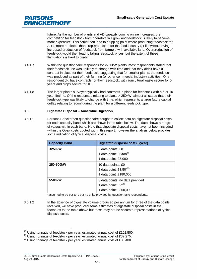
Small-scale Generation Cost Update
DECC Small-Scale Generation Costs Update V11 - FINAL.docx Prepared by Parsons BrinckerhoffAugust 2015 for Department of Energy and Climate Change
- 53 -
future. As the number of plants and AD capacity coming online increases, thecompetition for feedstock from operators will grow and feedstock is likely to becomemore expensive. This could then lead to a tipping point where producing feedstock forAD is more profitable than crop production for the food industry (or likewise), drivingincreased production of feedstock from farmers with available land. Overproduction offeedstock would then lead to falling feedstock prices, but the extent of thesefluctuations is hard to predict.
Within the questionnaire responses for <250kW plants, most respondents stated that3.4.1.7their feedstock use was unlikely to change with time and that they didn’t have acontract in place for their feedstock, suggesting that for smaller plants, the feedstockwas produced as part of their farming (or other commercial industry) activities. Onerespondent did have contracts for their feedstock, with agricultural waste secure for 5years and crops secure for 10.
The larger plants surveyed typically had contracts in place for feedstock with a 5 or 103.4.1.8year lifetime. Of the responses relating to plants > 250kW, almost all stated that theirfeedstock type was likely to change with time, which represents a large future capitaloutlay relating to reconfiguring the plant for a different feedstock type.
3.5 Digestate Disposal – Anaerobic Digestion
Parsons Brinckerhoff questionnaire sought to collect data on digestate disposal costs3.5.1.1for each capacity band which are shown in the table below. The data shows a rangeof values within each band. Note that digestate disposal costs have not been includedwithin the Opex costs quoted within this report, however the analysis below providessome indication of typical disposal costs.
Capacity Band Digestate disposal cost (£/year)
<250kW 2 data points: £01 data point: £5/ton18
1 data point: £7,000
250-500kW 10 data points: £01 data point: £3.50*19
1 data point: £180,000
>500kW 3 data points: no data provided1 data point: £2*20
1 data point: £200,000*assumed to be per ton, but no units provided by questionnaire respondents.
In the absence of digestate volume produced per annum for three of the data points3.5.1.2received, we have produced some estimates of digestate disposal costs in thefootnotes to the table above but these may not be accurate representations of typicaldisposal costs.
18 Using tonnage of feedstock per year, estimated annual cost of £102,500.19 Using tonnage of feedstock per year, estimated annual cost of £37,275.20 Using tonnage of feedstock per year, estimated annual cost of £30,400.

Small-scale Generation Cost Update
DECC Small-Scale Generation Costs Update V11 - FINAL.docx Prepared by Parsons BrinckerhoffAugust 2015 for Department of Energy and Climate Change
- 54 -
The data suggests that for plants <500kW, digestate disposal costs are generally3.5.1.3close to £0, possibly as operators of these plants use the digestate as part of theirown farming (or other small industrial) activities or as revenues from selling digestateare cancelled out by transport costs. This is supported by WRAP’s 2013 report intodigestate distribution models21and their Anaerobic Digestate Financial ImpactAssessment22.
For plants >500kW, the two data points are equivalent to costs of £47/kW/yr and3.5.1.4£71/kW/yr. In the absence of a larger dataset, the average of these values could beused i.e. £59/kW/yr. The higher costs for this band may be a result of larger plantsthat have more digestate to dispose of and so find it harder to achieve zero- or low-cost local disposal.
3.6 Anti-dumping scenarios – Solar PV
In June 2013, the European Commission announced that provisional anti-dumping3.6.1.1duties would be imposed on imports of solar panels, cells and wafers from China.These duties were imposed as a way of ensuring fair and competitive prices acrossthe countries of the EU in relation to the solar PV industry.
The anti-dumping duties were the result of an investigation that the Commission3.6.1.2launched in 2012, in response to a complaint by the European Pro Sun coalition, agroup of 25 European solar panel manufacturers headed by the German-basedSolarWorld.
In December 2013, the European Council backed the proposal to impose anti-3.6.1.3dumping and anti-subsidy measures on imports of solar panels from China. Theduties were fixed at an average of 47.7% and would apply for two years as of 6December 201323. The pact covers more than 90 Chinese exporters that have about60 percent of the EU solar-panel market. Participating producers include Yingli,Suntech, Trina, Jiangsu Aide Solar Energy Technology Co., Delsolar (Wujiang) Ltd.,ERA Solar Co., Jiangsu Green Power PV Co. and Konca Solar Cell Co.
These duties ensure a “minimum price” for solar panels, cells and wafers is seen3.6.1.4across Europe. The forecast Capex costs in Section 2 assume that the anti-dumpingduties will remain in place and stable up to, or past, 2021.
DECC have requested that these Capex costs are also forecast assuming that the3.6.1.5anti-dumping duties are revoked following review in December 2015 (with lowerpriced Chinese panels available for installation from January 2016).
The figures given in section 2.2 of this report assume that anti-dumping duties remain3.6.1.6in place. The following calculations assume that anti-dumping measures are revokedin December 2015.
During the final quarter of 2014, it was estimated that the delivered price of Tier 13.6.1.7modules from China were approximately USD0.57/W compared to the EU delivered
21 Available athttp://www.wrap.org.uk/sites/files/wrap/Digestate%20distribution%20models%20report.pdf22 Published 2009, Available at http://www.organics-recycling.org.uk/uploads/category1060/Financial_impact_assessment_for_anaerobic_digestate.pdf23 http://europa.eu/rapid/press-release_IP-13-1190_en.htm

Small-scale Generation Cost Update
DECC Small-Scale Generation Costs Update V11 - FINAL.docx Prepared by Parsons BrinckerhoffAugust 2015 for Department of Energy and Climate Change
- 55 -
price of USD0.65/W24. As the Chinese panels are subject to a 47.7% duty, it isreasonable to assume that relaxed anti-dumping laws would yield a delivered price ofUSD0.39/W (during the final quarter of 2014).
Parsons Brinckerhoff have retained the forecast linear decrease in PV panel costs in3.6.1.8line with that demonstrated in the IRENA report and discussed in 2.2.5.1, but haveassumed a scenario that from January 2016, all solar PV installations in the UnitedKingdom are built using Chinese panels imported free from the 47.7% duty. Thebalance of plant cost has not been changed as a relaxation of these duties would notaffect this cost.
Using this methodology, the forecast Capex costs would be as follows:3.6.1.9
Capacity Band March2015
Jan2016
Jan2017
Jan2018
Jan2019
Jan2020
Jan2021
Jan2022
<4kW new build 1,688 1,426 1,409 1,392 1,376 1,360 1,344 1,328
<4kW retrofit 1,688 1,426 1,409 1,392 1,376 1,360 1,344 1,328
4 - 10kW new build 1,442 1,225 1,211 1,197 1,183 1,169 1,156 1,142
4 - 10kW retrofit 1,442 1,225 1,211 1,197 1,183 1,169 1,156 1,142
10 - 50kW new build 1,250 1,062 1,050 1,037 1,025 1,013 1,002 990
10 - 50kW retrofit 1,250 1,062 1,050 1,037 1,025 1,013 1,002 990
50-150kW new build 1,173 997 985 974 962 951 940 930
50-150kW retrofit 1,173 997 985 974 962 951 940 930
150-250kW new build 1,072 910 900 889 879 869 859 849
150-250kW retrofit 1,072 910 900 889 879 869 859 849
250-5000kW new build 1,021 868 858 848 838 828 819 809
250-5000kW retrofit 1,021 868 858 848 838 828 819 809
Stand alone 1,039 883 873 862 852 842 833 823
Agg <4 1,519 1,284 1,268 1,253 1,238 1,224 1,209 1,195
Agg >4 1,298 1,103 1,090 1,077 1,064 1,052 1,040 1,028
Figure 3:5 below shows the forecast Capex costs for solar PV assuming that anti-3.6.1.10dumping duties are not relaxed in December 2015. This represents the base case.
24 http://www.greentechmedia.com/articles/read/regional-pv-module-prices-vary-by-as-much-as-0.16-w

Small-scale Generation Cost Update
DECC Small-Scale Generation Costs Update V11 - FINAL.docx Prepared by Parsons BrinckerhoffAugust 2015 for Department of Energy and Climate Change
- 56 -
Figure 3:5 Forecast solar PV Panel Capex assuming anti-dumping duties are not relaxed
Figure 3:6 below shows the base case in relation to the “relaxation” scenario, with one3.6.1.11system type displayed for simplicity. As shown, relaxation of the laws would trigger asudden decrease in Capex costs as cheaper panels are available for installation.Over time, there would be gradual but minor convergence of the two cases as thepanel price becomes a smaller percentage of the total Capex cost.
A more realistic, central case if anti-dumping measures were relaxed would probably3.6.1.12lie between the two cases given below.
-
100
200
300
400
500
600
700
800
2014 2015 2016 2017 2018 2019 2020 2021 2022 2023
Fore
cast
Pane
lCap
ex(£
/kW
)
Year
<4kW new build <4kW retrofit 4 - 10kW new build
4 - 10kW retrofit 10 - 50kW new build 10 - 50kW retrofit
50-150kW new build 50-150kW retrofit 150-250kW new build
150-250kW retrofit 250-5000kW new build 250-5000kW retrofit
Stand alone Agg <4 Agg >4
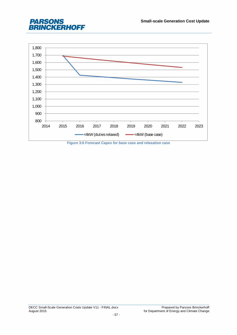
Small-scale Generation Cost Update
DECC Small-Scale Generation Costs Update V11 - FINAL.docx Prepared by Parsons BrinckerhoffAugust 2015 for Department of Energy and Climate Change
- 57 -
Figure 3:6 Forecast Capex for base case and relaxation case
800
900
1,000
1,100
1,200
1,300
1,400
1,500
1,600
1,700
1,800
2014 2015 2016 2017 2018 2019 2020 2021 2022 2023
<4kW (duties relaxed) <4kW (base case)

Small-scale Generation Cost Update
DECC Small-Scale Generation Costs Update V11 - FINAL.docx Prepared by Parsons BrinckerhoffAugust 2015 for Department of Energy and Climate Change
- 58 -
4 QUALITATIVE ASSESSMENT
4.1 Introduction
In addition to the data-gathering exercise, all consultees were asked a number of4.1.1.1questions in relation to the technologies covered by the FIT and their perception ofthe future of these markets and barriers to deployment. The following sectiondiscusses the issues raised and attempts to form a sector-wide view of the industryand its future challenges.
The following narrative represents views expressed in the questionnaire responses4.1.1.2only and does not necessarily represent the views of DECC or Parsons Brinckerhoff.
4.2 Solar – domestic
When planning your solar PV installation, was it more important for you to dosomething that saved you money (through reduced energy bills/FIT), or that couldbenefit the environment? Why?
While domestic installers all stated the decision to install solar panels was based on a4.2.1.2desire to benefit the environment, all respondents agreed that saving money was alsoan important factor and that both elements had to align. One homeowneracknowledged that their payback time was likely to be much longer than firstanticipated, but a second homeowner stated that the FIT allows them to earn a betterreturn on capital than current bank interest rates.
Any other comments?
One homeowner suggested a “fast FIT” scheme for commercial installations in order4.2.1.3to boost the market, where a higher tariff is paid for a shorter length of time in order tospeed up payback and increase return on investment, with a reduced FIT for theremainder of the plant’s lifetime. This would help to unlock the commercial solarmarket and reduce financial risk.
4.3 Solar – commercial
Very few qualitative responses were received in relation to solar PV and the views4.3.1.1outlined below reflect those responses received. Attempts to obtain additionalinformation in relation to the following questions were often passed over bystakeholders.
How do you see the solar PV market changing over the next 5 years?
Commercial solar developers discussed the recent move from RO to CfDs and the4.3.1.2indirect impact that this will have on FIT customers. The understanding is that as solar(with a cost of $157/MWh) has been grouped with onshore wind (with a cost of$88/MWh), solar has now become non-competitive in the CfD scheme. This will inturn reduce the deployment of large-scale solar PV arrays, which could stall thedevelopment of the technology, reducing the opportunity for cost reduction of thetechnology, materials and equipment. As cost reductions in the large scale marketfeed into the domestic and FIT markets, all will suffer.
A number of additional stakeholders also explained to Parsons Brinckerhoff and4.3.1.3DECC that the solar PV market in the UK was rapidly moving towards a subsidy freefuture, with grid parity reached in 2018-2020.

Small-scale Generation Cost Update
DECC Small-Scale Generation Costs Update V11 - FINAL.docx Prepared by Parsons BrinckerhoffAugust 2015 for Department of Energy and Climate Change
- 59 -
What is your opinion on site availability? Are suitable sites still available fordevelopment?
Developer consultees agree that solar PV is one of the least controversial forms of4.3.1.4energy production in the UK and should be encouraged, but that FIT tariff bandinghas made ground-mounted sites unattractive and not financially viable. While rooftopsites are available, the number of suitable sites is finite.
4.4 Wind
How do you see the onshore wind market changing over the next 5 years?
Technology manufacturers and project developers agree that the market will shift, but4.4.1.2disagree with regards to which direction. While some respondents believe that theonshore wind market will become more reliant on small scale/micro generation with asmaller visual impact, deployed in greater numbers for distributed generation, othersbelieve the market will shift towards larger turbines with a lower cost of energy. Onemanufacturer and a number of developers suggested that the market will diminish tovery low levels due to the lack of viable incentives and a second stated that with anongoing tariff degression of ~20% per year, the market is expected to effectively die inthe very near future without intervention. Grid capacity, especially for turbinedevelopments above 50kW, was highlighted as a roadblock across most parts of thecountry with a suggestion that attention should be given towards supporting thecommercial development of energy storage technologies – an idea supported bydevelopers.
Developers suggested that with the current degression levels, a future for small to4.4.1.3medium scale projects between 500kW and 20MW looks unlikely. Discussion touchedon investment in the wind industry and the difficulties in selling projects to investors ifthe FIT rate drops below the current levels as investors will look elsewhere for higheryields. Consolidation of companies in the industry as the market tightens andhenceforth a notable shrinkage of the industry was also suggested by a number ofconsultees, making achieving 2030 decarbonisation targets more difficult.
Developers and non-domestic respondents both suggested that community4.4.1.4ownership could become more prevalent, especially in relation to single turbine siteswith a high energy usage or near small settlements. However, a second developerviewed that the continuous FIT degression makes progressing further single turbineand small cluster projects challenging when the greatest remaining potential in the UKis for these types of developments. Expansion or repowering upgrades of existingwind farms may take place instead of the development of new sites.
Developers discussed how the tariff bands do not best reflect available technology,4.4.1.5resulting in a number of single turbine projects having to be de-rated in order to makethem viable.
Would you have installed a higher capacity turbine(s) at any of your sites if the tariffbanding was structured differently? If yes, at which site(s)? What capacity would youhave installed?
Opinion was split equally in response to this question. While a community consultee4.4.1.6confirmed that they would not have installed a higher capacity turbine as they had to“live with” their project and would not want a taller turbine, a non-domestic respondentstated they would have installed a 900kW or 1.5kW turbine in place of their 500kW ifthe tariff bands were structured differently.

Small-scale Generation Cost Update
DECC Small-Scale Generation Costs Update V11 - FINAL.docx Prepared by Parsons BrinckerhoffAugust 2015 for Department of Energy and Climate Change
- 60 -
Responses to this question were largely site specific – for lower wind speed sites,4.4.1.7developers would install larger turbines or more than one turbine, although highcapital costs make it difficult to do in every case. One developer said they would notchange any of the sites they had previously developed, but would have to installlarger turbines on any new sites in order to make their projects economically viable.However, one developer disagreed and stated that banding should favour microgeneration as this supports the many, not the minority.
A number of responses mentioned projects with an installed capacity of 500kW,4.4.1.8stating that higher capacity turbines would have been installed on these sites hadthere been higher tariffs available. One manufacturer and developer discussed indetail how schemes are developed at the upper ends of the capacity bands asdefined by the FIT, which then results in turbine manufacturers manufacturingturbines sized specifically for the upper ends of the bands (500kW and 1.5MW).Developers also push projects to the high ends of these bands to ensure least riskand higher returns. This was reflected in the data gathered under this project with alarge number of projects with an installed capacity of 500kW.
What is your opinion on site availability? Are suitable sites still available fordevelopment?
The majority of consultees agreed that sites are becoming more difficult to find with4.4.1.9high enough wind speeds (7.0 – 7.5m/s) to hit the hurdle rates required, with gridavailability and without aviation radar constraints. Where sites are available, smallerchances of getting through planning and increasing pressure on landowners fromanti-wind groups contribute to fewer planning applications being submitted. Acommunity consultee confirmed that their recent experience showed that most siteshave already been surveyed with options to develop already secured and that newsites are very difficult to find.
The lack of available grid capacity was discussed in detail, as for hydro above. Some4.4.1.10suggestions were made that micro generation may be the only way forward as theconstraints are less limiting.
A group of consultees agreed that suitable sites were available although the4.4.1.11degression of the FIT makes it financially unattractive for potential owners to developthe sites. One respondent suggested that grid upgrades, aviation improvements andincreased community involvement had the potential to open up more sites in thefuture, potentially for single and small cluster developments.
How do you see hurdle rates evolving over the next five years?
All respondents agreed that hurdle rates will fall over the next five years, although the4.4.1.12exact percentage they will fall to was not discussed. Manufacturers and developerssuggested they would reduce by a “couple of percent” and that they would need todecrease in order for them to continue to work in the market. Respondents stated thatthe reduction in these hurdle rates (especially if combined with an increase in interestrates) would cause investors to leave the space, a huge reduction in the number ofplanning applications and/or a complete cease in the development of new sites andthe potential demise of the small wind industry.
A non-domestic respondent suggested that hurdle rates would decrease given4.4.1.13emerging funding methods, such as crowdfunding. A community respondentconfirmed that developers and investors will need to accept lower returns if they areto continue developing turbines onshore.

Small-scale Generation Cost Update
DECC Small-Scale Generation Costs Update V11 - FINAL.docx Prepared by Parsons BrinckerhoffAugust 2015 for Department of Energy and Climate Change
- 61 -
Parsons Brinckerhoff believes that some of these responses discuss ‘hurdle rates’4.4.1.14where ‘return on investment’ should instead be used.
How do project constraints or cost/financing implications vary across community-led/shared ownership projects and commercial projects?
Responses to this question were largely in agreement to those given in relation to4.4.1.15community hydro projects. Developers confirmed that community partnership projectsare considerably more time consuming to develop and that funding is difficult tosecure. However, as for wind, no real evidence was provided as part of this datacollection exercise that suggested community projects had higher capital or operatingcosts than commercial or developer led projects.
Shared, or community ownership schemes are not considered attractive by FIT4.4.1.16developers due to the up-front costs of involving the community prior to achievingconsent, when there is no guarantee that community support will help achieveconsent and solely community-owned schemes may have difficulties raising capitaland navigating the planning and construction phases of the development. Generally,commercial projects will move through the planning and feasibility stages of theproject much faster.
Any other comments?
One developer suggested that the <500kW FIT band is too generous, with the4.4.1.17>1.5MW band unviable since the first degression. Adjustments of these bands wouldensure a sensible long-term future for the onshore FIT wind market. Otherrespondents disagreed, stating that the removal of the 15kW banding following theprevious consultation has resulted in an 80% decline in micro-generation installationsand that as turbines >50kW do not have to go through product certification and canbe pre-accredited, the sub <50kW market is being heavily penalised with no FITadjustment to compensate for this. It was also highlighted that 80% ofmicrogeneration turbines installed in the UK were manufactured in the UK, whereas90% of >50kW turbines installed in the UK were imported, and that a tariff change isneeded in order to support the UK manufacturing industry.
4.5 Hydro
How do you see the hydroelectric market changing over the next 5 years?
Domestic respondents to this survey agreed that further cuts in the FIT would affect4.5.1.2further uptake in this technology, but disagreed over the future Capex costs relation tohydro – while one domestic consultee suggested that technology improvementswould make systems easier and cheaper to install, another discussed the lack ofeconomies of scale relating to hydro installations, and how rising material and labourcosts do not corroborate with tariff degression. Domestic respondents also touchedon the deterring element of high development and planning costs and the regulationsimposed by the Environment Agency around hydro generation, calling them“restrictive and unsubstantiated”.
Non-domestic respondents were largely in agreement about the future of the4.5.1.3hydroelectric market, suggesting that the market may not improve with the reductionin the FIT, increasingly challenging regulations and limited future cost reductions inthe technology. They agreed that there is always likely to be some demand for thetechnology, but that any further reduction in the FIT will limit the construction of futureschemes.
Small-scale Generation Cost Update
DECC Small-Scale Generation Costs Update V11 - FINAL.docx Prepared by Parsons BrinckerhoffAugust 2015 for Department of Energy and Climate Change
- 62 -
Developers varied in their responses to this question. While some developers4.5.1.4suggested that the market has slowed in the last 12 months and the level of newenquiries has fallen dramatically, others suggested that the FIT has been generallypositive for hydro – stimulating investment without over-compensating investors.Almost all developers were in agreement that the degression mechanism willsignificantly curtail, or potentially collapse future deployment and that this has beenwitnessed in the small, domestic scale projects (<15kW). Regulatory barriers from theEnvironment Agency (EA) and inflation have increased the capital costs of hydro asthe FIT has decreased and the decreasing interest in early stage development since2014 is a result of this.
Developers also suggested that 2015 and 2016 may see an unprecedented boom in4.5.1.5construction, with up to 40MW deployed each year but following that, construction willfall dramatically, returning to pre-FIT levels of deployment. Largely, hydro will fall wayshort of its deployment potential given a lack of funding sources, degression ratesbased on pre-accreditation and lack of build out and a suggested bias towards otherrenewable energy technologies.
Utility scale respondents agreed that a surge of construction in the coming years is4.5.1.6likely, but FIT degression will ensure that very few < 5MW sites will be developedbeyond 2018.
Specialist consultancies who were approached during this study suggested that the4.5.1.7market would see a move towards a larger number of community projects.Respondents also stated that while micro-hydro (<100kW) has enormous potentialacross the UK, the levels of bureaucracy in place restrict uptake and limit interestfrom commercial manufacturers and installers.
What is your opinion on site availability? Are suitable sites still available fordevelopment?
Domestic respondents agreed that there are thousands of sites still available,4.5.1.8particularly on old mill sites, but that many are difficult to develop. The comments fromnon-domestic respondents echoed these thoughts by confirming that there are plentyof small (<100kW) sites still available, but that most are un-economic to develop,possibly as a result of high consenting costs, and are restricted by EA datarequirements and reduced permissible water flows.
Comments from developers agreed that a substantial number of technically viable4.5.1.9sites are still available, but that FIT degression has pushed the marginal ones out ofrange and the feasibility of identified opportunities is dependent upon adequatesupport mechanisms being in place. A key comment raised by many respondentsrelates to the grid and the lack of cohesion between grid connection dates and thetwo year FIT build window. Of the sites that are yet to be exploited, many lie in areaswith severe grid constraints where upgrades are planned but would not be completein time for connection under the FIT mechanism. Some developers also discussedtheir lack of confidence in the FIT regime affecting their willingness to develop furthersites. However, one developer did confirm that viable sites are still available at thecurrent FIT levels, but that viability significantly decreases once total degression inFIT rates exceeds 20%.
Utility-scale respondents largely agreed with these views and confirmed that they own4.5.1.10a development pipeline of schemes, however unless an improvement in supportmechanisms happened, it is unlikely they would be constructed.

Small-scale Generation Cost Update
DECC Small-Scale Generation Costs Update V11 - FINAL.docx Prepared by Parsons BrinckerhoffAugust 2015 for Department of Energy and Climate Change
- 63 -
How do you see hurdle rates evolving over the next 5 years?
Developers were largely in agreements that the hurdle rates are already as low as4.5.1.11viable and will only increase as the cost of finance increases. 8% was given as theminimum return on equity required by professional investors with a view that this willnot evolve significantly over the next 5 years unless slightly upwards as projectsbecome more challenging and investment is instead made into other industries with amore attractive risk/reward profile. Another respondent suggested that as interestrates are currently at a historical low, it seems inevitable that they will only rise againin years to come, but that the cost of finance for small-scale hydro is notcomparatively low. It was suggested in the responses that tariff degression has takenFIT levels to a point where it is not possible to meet existing hurdle rates, hence thecessation of new project development. As hydro is civil engineering led, technologyimprovements will have little impact on the cost of installation and therefore bigchanges in finance required is unlikely.
A consultant respondent agreed with the views of the developers and suggested that4.5.1.12hurdle rates for many schemes are now on the threshold of private funding.
Parsons Brinckerhoff believes that some of these responses discuss ‘hurdle rates’4.5.1.13where ‘return on investment’ should instead be used.
How do project constraints or cost/financing implications vary across community-led/shared ownership projects and commercial projects?
Developers largely agreed that it is dependent on the source of funding. If self-4.5.1.14investment or low cost funding is available for community schemes, they can developprojects with lower hurdle rates. While community projects may appear easier todevelop, it is perceived that they seriously underperform in comparison to commercialprojects, and for a given project, a community-led approach will generally be moreexpensive, more complex, will take longer and be riskier than the same project led bya commercial developer. However, the respondents concluded that community andcommercial schemes are facing the same challenges – obtaining finance, FITdegression, the pressures of a 2 year build window, grid availability and contractoravailability during the short-term construction ‘boom’ resulting from the pre-accreditation/degression effect. One developer noted that while there is an impressionthat a wave of new money has entered the hydro sector, this is primarily equityfinance which is not what communities or commercial developers are seeking.
A consultant believed that project IRRs are becoming too low for most commercial4.5.1.15investments and as such, ‘low-return’ community schemes could become the norm infuture. A non-domestic respondent explained that for community projects, it is moredifficult to obtain the initial high-risk financing for development works and agreed withthe developers that hydropower is a challenging technology for communityorganisations to develop; however, it was suggested that local authorities may beideally placed to develop schemes as they have both land availability and sources ofcapital.
Generally, no real evidence was provided as part of this data collection exercise that4.5.1.16suggested community projects had higher capital or operating costs than commercialor developer led projects.
Small-scale Generation Cost Update
DECC Small-Scale Generation Costs Update V11 - FINAL.docx Prepared by Parsons BrinckerhoffAugust 2015 for Department of Energy and Climate Change
- 64 -
Any other comments?
One domestic respondent suggested that the FIT payments should be stepped by4.5.1.17number of units produced rather than installed capacity in order to encourage ownersto produce the maximum units they can. Suggestions were also made to change theEA regulations in order to make them more flexible and site-specific.
Developer responses suggested that while hydro faces a cliff edge at the end of 2016,4.5.1.18there is a similar situation present for all renewable energy sectors whereby a falseimpression is being given by what is happening at the construction end of thedevelopment pipeline. Focus should instead be fixed on the other end of the pipelinewith sufficient encouragement given to stimulate the speculative investment that isnecessary if the growth in renewable technologies is to continue.
Consultant respondents suggested that small (<15kW) self-funded domestic schemes4.5.1.19are likely to stop being installed at all, and that <10kW are currently no longerfinancially viable for the majority of sites. A utility respondent also commented thattaxes relating to hydro projects will be elevated by the lack of any tax relief onsubstantial proportions of capital expenditure.
4.6 Anaerobic Digestion (AD)
How do you see the anaerobic digestion market changing over the next 5 years?
Respondents were concerned by a lack of tariff certainty (and quick tariff degression)4.6.1.2and the impact this has had on availability of funding for the projects. Respondentsfelt this was a particular issue for sub 500kW systems and was having an impact onmixed agricultural waste and crop input systems for farms. One respondent notedthat larger-scale, waste based projects may remain viable in the short term. Thissame respondent noted that tariff degression to date has proceeded at a faster ratethan any reduction in project costs or required return rates.
One respondent raised grid constraints as a major issue for the future development of4.6.1.3the CHP based AD market, and noted that restricted export to the grid meant projectscould not be funded. The same respondent commented that FIT rates need to beadequate to compensate for restricted generation (ie. only exporting at night andduring the winter) when it could act as a balancing mechanism for solar PV.
One respondent noted the oversupply of digesters and shortage of feedstock as a key4.6.1.4issue for market development.
One respondent noted that downward pressure on gate fees is likely to constrain4.6.1.5growth in the market in the medium term.
How do you see the gate fee market evolving over the next 5 years?
The general consensus of respondents was that the gate fee market will fall4.6.1.6significantly, and will ultimately be a cost rather than an income for the projects.
One respondent attributed the fall in gate fees to certain areas having overcapacity of4.6.1.7processing sites, slow progress on capture rates and delay in introducing a ban onfood waste to landfill.
One respondent noted that their expectation was that the food waste gate price will4.6.1.8drop through competition to less than £15 per tonne and any additional charges will

Small-scale Generation Cost Update
DECC Small-Scale Generation Costs Update V11 - FINAL.docx Prepared by Parsons BrinckerhoffAugust 2015 for Department of Energy and Climate Change
- 65 -
be commensurate with the level of de-packaging or process difficulty associated withit.
How secure is your current feedstock supply? Do you foresee any problems withavailability? How do you think feedstock usage across the market will change over thenext 5 years?
The general consensus from respondents was that agricultural feedstock is secure as4.6.1.9it’s produced by local livestock and grown on the farm and farm-based AD can takeadvantage of market oversupply which are readily available at a low gate price.Security of the overall feedstock ranged from very secure to partially secure.
One respondent noted that for projects that use waste feedstocks, long term supply4.6.1.10contracts are increasingly difficult to obtain, meaning that project risks are increasedwhich has increased the hurdle rate.
How do you see hurdle rates evolving over the next 5 years?
Responses to this question varied slightly but the general content is summarized4.6.1.11below:
· The hurdle rate is unlikely to change;
· The hurdle rate is unlikely to drop significantly due to the operational complexityof AD projects and the risks around feedstock supply and digestate disposal;
· In the near term, hurdle rates may actually increase due to the removal ofrelatively low cost Enterprise Investment Scheme and Venture Capital Trustsfunding from the market;
· Debt finance will become harder to secure as some projects fail due to lack offeedstock and technical problems;
· Investors will always look for the maximum return.
One respondent noted that farm systems with a higher level of equity or asset4.6.1.12recourse are more influenced by overall estate / farm sustainability and long termfinancial requirements, however the current degression of the FIT and uncertainty onthe Renewable Heat Incentive has meant that these systems may not currently beviable.
Any other comments?
One respondent noted that although there is still a great deal of interest in the AD4.6.1.13sector, very few projects are now managing to get funding. In many cases the initialfarm based plants are requiring substantial adjustments to meet the permitrequirement which were not made clear in the initial delivery by the technologysuppliers, as the farmers were not used to the requirements of the waste permittingside.
The same respondent noted that feedstock costs have also in most cases exceeded4.6.1.14what was initially envisaged as has the level of management for farm scale systemsand it may be that some of the current plants do not achieve (by a significant margin)the 20 year operational plan. There are many excellent farm scale plants that are runby dedicated and informed individuals who are clear that if the opportunity was tocome up again with the current degression that they would not go down the AD routein the current climate.

Small-scale Generation Cost Update
DECC Small-Scale Generation Costs Update V11 - FINAL.docx Prepared by Parsons BrinckerhoffAugust 2015 for Department of Energy and Climate Change
- 66 -
ANNEX A – WEIGHTINGS

Small-scale Generation Cost Update
DECC Small-Scale Generation Costs Update V11 - FINAL.docx Prepared by Parsons BrinckerhoffAugust 2015 for Department of Energy and Climate Change
- 67 -
Solar Capex
Year Installed
2012 0.7 Somewhat higher Feed-in Tariffs available during these yearsmeans Capex prices were also skewed to ensure an 8-10 yearpayback period.2013 0.8
2014 1.0
2015 1.0
Data Source
Domestic Homeowner 1.0 Unlikely to invest in further projects and as such, data source islikely to be accurate.Community Group 1.0
Other 0.95 Adjusted for bias.
Project Type
Existing/Built 1.0
Example 0.8-1.2 Adjusted upwards or downwards by 20% depending onParsons Brinkerhoff’s view of how realistic estimated prices are.
Solar Opex
Data Source
Domestic Homeowner 1.0 Unlikely to invest in further projects and as such, data source islikely to be accurate.Community Group 1.0
Other 0.95 Adjusted for bias.
Project Type
Existing/Built 1.0
Example 0.5 Sources provided examples were largely unsure of Opex pricesas projects are often transferred once commissioned.

Small-scale Generation Cost Update
DECC Small-Scale Generation Costs Update V11 - FINAL.docx Prepared by Parsons BrinckerhoffAugust 2015 for Department of Energy and Climate Change
- 68 -
Wind Capex
Year Installed
2010 0.85 Weighted reflective of the higher project costs prior toDecember 2012.2011 0.85
2012 0.85
2013 0.95 Weighted reflective of the higher project costs prior to 2014.
2014 1.0
2015 1.0
Data Source
Domestic Homeowner 1.0 Unlikely to invest in further projects and as such, data source islikely to be accurate.Community Group 1.0
Other 0.95 Adjusted for bias.
Project Type
Existing/Built 1.0
Example/Anticipated 0.9-1.1 Adjusted upwards or downwards by 10% depending onParsons Brinkerhoff’s view of how realistic estimated prices are.
Wind Opex
Data Source
Domestic Homeowner 1.0 Unlikely to invest in further projects and as such, data source islikely to be accurate.Community Group 1.0
Other 0.95 Adjusted for bias.
Project Type
Existing/Built 1.0
Example 0.95-1.05
Sources provided examples were largely unsure of Opex pricesas projects are often transferred once commissioned.

Small-scale Generation Cost Update
DECC Small-Scale Generation Costs Update V11 - FINAL.docx Prepared by Parsons BrinckerhoffAugust 2015 for Department of Energy and Climate Change
- 69 -
Hydro Capex
Year Installed
2010 1.05 Adjusted due to the lower FIT rate prior to 2012.
2011 1.05
2012 1.05
2013 1.0
2014 1.0
2015 1.0
2016 1.0
2017 0.95 Adjusted for uncertainty around predicted costs.
Data Source
Domestic Homeowner 1.0 Unlikely to invest in further projects and as such, data source islikely to be accurate.Community Group 1.0
Other 0.95 Adjusted for bias.
Project Type
Existing/Built 1.0
Example 0.8-1.2 Adjusted upwards or downwards by 20% depending onParsons Brinkerhoff’s view of how realistic estimated prices are.
Hydro Opex
Data Source
Domestic Homeowner 1.0 Unlikely to invest in further projects and as such, data source islikely to be accurate.Community Group 1.0
Other 0.95 Adjusted for bias.
Project Type
Existing/Built 1.0
Example 0.5 Sources provided examples were largely unsure of Opex pricesas projects are often transferred once commissioned.

Small-scale Generation Cost Update
DECC Small-Scale Generation Costs Update V11 - FINAL.docx Prepared by Parsons BrinckerhoffAugust 2015 for Department of Energy and Climate Change
- 70 -
Anaerobic Digestion Capex
Year Installed
2009 1.0
2010 1.0
2011 0.9 Adjusted to reflect increased project costs during this period.
2012 0.75
2013 0.75
2014 1.0
2015 1.0
Data Source
Domestic Homeowner 1.0 Unlikely to invest in further projects and as such, data source islikely to be accurate.Community Group 1.0
Other 0.95 Adjusted for bias.
Project Type
Existing/Built 1.0
Example 0.8-1.2 Adjusted upwards or downwards by 20% depending onParsons Brinkerhoff’s view of how realistic estimated prices are.
Anaerobic Digestion Opex
Data Source
Domestic Homeowner 1.0 Unlikely to invest in further projects and as such, data source islikely to be accurate.Community Group 1.0
Other 0.95 Adjusted for bias.
Project Type
Existing/Built 1.0

Small-scale Generation Cost Update
DECC Small-Scale Generation Costs Update V11 - FINAL.docx Prepared by Parsons BrinckerhoffAugust 2015 for Department of Energy and Climate Change
- 71 -
ANNEX B – QUESTIONNAIRES

NameCompanyEmailTelephoneCompany Type
Notes for completion of questionnaire
4. Installation cost should be the cost at date commissioned.5. Grid connection costs should include any upfront connection payment and substation/transformer costs but exclude pre-connection securities.
11. Please add more columns or rows to tables as necessary.12. If you wish to clarify any of your answers, please use the comments box at the bottom of this page.
1 2 3 4 5 6 7 8 9 10Project Type
Installed capacity (kW)
Date commissioned
Installation Cost (CAPEX) (£/kWp)
inc. VAT? (Y/N)
Landownership type
CAPEX costs pertaining to land (i.e. purchase cost/total land rental during construction) (£/kW)
Grid connection costs (£)
Grid connection type
Distance from project to grid connection (km)
Turbine cost excl. VAT (£)
Tubine Manufacturer/Model
Hub height above Ground Level (m)
Rotor diameter (m)
Building mounted or mast mounted?
Fixed maintentance (OPEX) (£/kW/yr)
Variable maintentance (OPEX) (£/kWh)
If site is leased/rented, what are annual land costs? (£/kW)
Connection Use of System charges (£/kW/yr)
Where is the site located?
What is the site postcode?
What is the average wind speed on site?
Load Factor (%) - predicted
Load Factor (%) - actual
Export Fraction (%)
Have you signed a PPA agreement for the project?
If yes, what rate do you sell to the grid at? (p/kWh)
1 2 3 4 5 6 7 8 9 10What is your hurdle rate for this investment? (%)
What is the gearing of this project? (%)What is the cost of the debt? (%)
What is your required return on equity? (%)
What is the tenor of loan on this investment? (years)
What risks do you see as the main drivers for the decision to invest (or not) in this technology?
What is the useful project life of this investment? (Useful economic life for valuation purposes) (years)
What is your effective tax rate? (%)
How do you see the onshore wind market changing over the next 5 years?
Would you have installed a higher capacity turbine(s) at any of your sites if the tariff banding was structured differently? If yes, at which site(s)? What capacity would you have installed?
8. The 'hurdle rate' is the minimum expected project Internal Rate of Return (IRR) for investment in a generation asset realised over the life of the asset, at which investors will make a decision to proceed with the investment. Our preference would be to obtain this on a real, pre-tax basis; however should you chose to provide it on a nominal and/or post-tax basis, please indicate so either by adding a comment to the cell or by using the comment box at the bottom of this page.
10. The 'effective' tax rate is the implied tax rate on a project after accounting for the debt interest tax shield (if relevant) and capital allowances.
1. Please provide all costs as they were at the time they were incurred and do not adjust for inflation, but please state the year in which they were incurred. In other words, please express costs in real money terms of the year in which you incurred them. If you prefer to provide nominal costs (i.e. costs expressed in today's terms), please state the base year and which price index you are linking to (i.e. RPI, CPI, etc), either by adding a comment to the cell or by using the comment box at the bottom of this page.
ONSHORE WIND
If required, Parsons Brinckerhoff will keep your responses anonymous.
7. Export fraction is the average annual fraction of electricity generated by the project and exported to the grid.
9. 'Gearing' is defined as the proportion of debt in the project's capital structure; in other words it is the percentage of total project costs that is funded by debt.
FURTHER COMMENTS
Project
3. Installation (CAPEX) costs should include the design, procurement and construction costs (e.g. EPC costs) and equipment and civil works costs. They should NOT include owner's costs, grid connection costs or substation and/or transformer costs.
6. OPEX costs should include labour, planned maintenance and lifecycle replacement. They should not include land costs, property and business rates tax costs, rental and community benefit payments. Variable OPEX may also include water and/or chemical usage.
2. Rural projects are defined as those that are in open and exposed areas which are largely free of obstacles in all directions. Urban sites are within built-up areas and are likely to be quite close to buildings and other ground features.
TECHNICAL ANALYSIS
ECONOMIC ANALYSIS
Project

What is your opinion on site availability? Are suitable sites still available for development?
How do you see hurdle rates evolving over the next 5 years?
How do project constraints or cost/financing implications vary across community-led/shared ownership projects and commercial projects?
Any other comments?

NameCompanyEmailTelephoneCompany Type
Notes for completion of questionnaire
7. Grid connection costs should include any upfront connection payment and substation/transformer costs but exclude pre-connection securities.
13. Please add more columns or rows to tables as necessary.14. If you wish to clarify any of your answers, please use the comments box at the bottom of this page.
1 2 3 4 5 6 7 8 9 10Project Type
Installed capacity (kW)
Date commissioned
Installation Cost (CAPEX) (£/kWp)
inc. VAT? (Y/N)
Landownership type
CAPEX costs pertaining to land (i.e. purchase cost/total land rental during construction) (£/kW)
Grid connection costs (£)
Grid connection type
Where is the site located?
Distance from project to grid connection (km)
Fixed maintentance (OPEX) (£/kW/yr)
Variable maintenance (OPEX) (£/kWh)
If site is leased/rented, what are annual land costs? (£/kW)
Connection Use of System charges (£/kW/yr)
Panel Cost excl. VAT (£/kWp)
Panel Type (manufacturer/model)
Inverter Cost excl. VAT (£/kWp)
Inverter Type (manufacturer/model)
Load factor (%) - predicted
Load factor (%) - actual
Performance ratio - predicted
Performance ratio - actual
Export Fraction (%)
Have you signed a PPA agreement for the project?
If yes, what rate do you sell to the grid at? (p/kWh)
1 2 3 4 5 6 7 8 9 10
What is your hurdle rate for this investment? (%)
What is the gearing of this project? (%)
What is the cost of the debt? (%)
What is your required return on equity? (%)
What is the tenor of loan on this investment? (years)What risks do you see as the main drivers for the decision
to invest (or not) in this technology?
What is the useful project life of this investment? (Useful economic life for valuation purposes) (years)
What is your effective tax rate? (%)
How do you see the solar PV market changing over the next 5 years?
What is your opinion on site availability? Are suitable sites still available for development?
How do you see hurdle rates evolving over the next 5 years?
How do project constraints or cost/financing implications vary across community-led/shared ownership projects and commercial projects?
SOLAR PV
TECHNICAL ANALYSIS
ECONOMIC ANALYSIS
Project
8. OPEX costs should include labour, planned maintenance and lifecycle replacement. They should NOT include land costs, property and business rates tax costs, rental and community benefit payments. Variable OPEX may also include water and/or chemical usage.
2. For roof mounted solar, 'new build' should be selected as project type where panels were installed during the building of the house. 'Retrofit' should be chosen where panels were installed on the house at a later date.
5. Installation (CAPEX) costs should include the design, procurement and construction costs (e.g. EPC costs) and equipment and civil works costs. They should NOT include owner's costs, grid connection costs or substation and/or transformer costs.
3. A solar 'aggregator' is that defined as an organisation that develops/owns a large number of small projects that are treated as individual schemes under the FiT. If providing details on an 'aggregator' type project, please input costs as for the small, individual projects, not for the portfolio of projects as a whole.4. 'Building integrated PV' should be completed where photovoltaic materials have been used to replace conventional building materials in a structure (e.g. roof, skylights). This does NOT include roof mounted solar PV.
6. Installation cost (CAPEX) should be the cost at date commissioned.
If required, Parsons Brinckerhoff will keep your responses anonymous.
10. The 'hurdle rate' is the minimum expected project Internal Rate of Return (IRR) for investment in a generation asset realised over the life of the asset, at which investors will make a decision to proceed with the investment. Our preference would be to obtain this on a real, pre-tax basis; however should you chose to provide it on a nominal and/or post-tax basis, please indicate so either by adding a comment to the cell or by using the comment box at the bottom of this page.
Project
FURTHER COMMENTS
1. Please provide all costs as they were at the time they were incurred and do not adjust for inflation, but please state the year in which they were incurred. In other words, please express costs in real money terms of the year in which you incurred them. If you prefer to provide nominal costs (i.e. costs expressed in today's terms), please state the base year and which price index you are linking to (i.e. RPI, CPI, etc), either by adding a comment to the cell or by using the comment box at the bottom of this page.
11. 'Gearing' is defined as the proportion of debt in the project's capital structure; in other words it is the percentage of total project costs that is funded by debt.12. The 'effective' tax rate is the implied tax rate on a project after accounting for the debt interest tax shield (if relevant) and capital allowances.
9. Export fraction is the average annual fraction of electricity generated by the project and exported to the grid.

Any other comments?
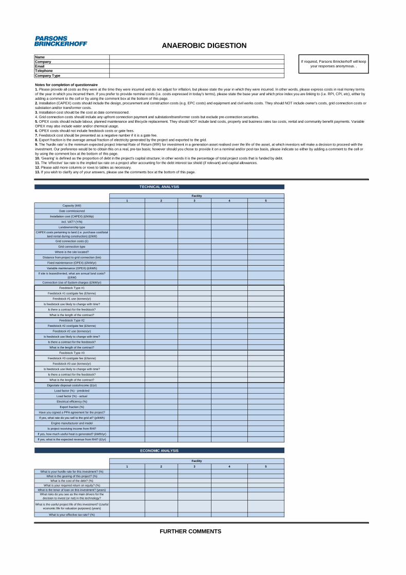
NameCompanyEmailTelephoneCompany Type
Notes for completion of questionnaire
3. Installation cost should be the cost at date commissioned.4. Grid connection costs should include any upfront connection payment and substation/transformer costs but exclude pre-connection securities.
6. OPEX costs should not include feedstock costs or gate fees.7. Feedstock cost should be presented as a negative number if it is a gate fee.
12. Please add more columns or rows to tables as necessary.13. If you wish to clarify any of your answers, please use the comments box at the bottom of this page.
1 2 3 4 5Capacity (kW)
Date commissioned
Installation cost (CAPEX) (£/kWp)
incl. VAT? (Y/N)
Landownership type
CAPEX costs pertaining to land (i.e. purchase cost/total land rental during construction) (£/kW)
Grid connection costs (£)
Grid connection type
Where is the site located?
Distance from project to grid connection (km)
Fixed maintentance (OPEX) (£/kW/yr)
Variable maintenance (OPEX) (£/kWh)
If site is leased/rented, what are annual land costs? (£/kW)
Connection Use of System charges (£/kW/yr)
Feedstock Type #1
Feedstock #1 cost/gate fee (£/tonne)
Feedstock #1 use (tonnes/yr)
Is feedstock use likely to change with time?
Is there a contract for the feedstock?
What is the length of the contract?
Feedstock Type #2
Feedstock #2 cost/gate fee (£/tonne)
Feedstock #2 use (tonnes/yr)
Is feedstock use likely to change with time?
Is there a contract for the feedstock?
What is the length of the contract?
Feedstock Type #3
Feedstock #3 cost/gate fee (£/tonne)
Feedstock #3 use (tonnes/yr)
Is feedstock use likely to change with time?
Is there a contract for the feedstock?
What is the length of the contract?
Digestate disposal costs/income (£/yr)
Load factor (%) - predicted
Load factor (%) - actual
Electrical efficiency (%)
Export fraction (%)
Have you signed a PPA agreement for the project?
If yes, what rate do you sell to the grid at? (p/kWh)
Engine manufacturer and model
Is project receiving income from RHI?
If yes, how much useful heat is generated? (kWth/yr)
If yes, what is the expected revenue from RHI? (£/yr)
1 2 3 4 5What is your hurdle rate for this investment? (%)
What is the gearing of this project? (%)What is the cost of the debt? (%)
What is your required return on equity? (%)What is the tenor of loan on this investment? (years)
What risks do you see as the main drivers for the decision to invest (or not) in this technology?
What is the useful project life of this investment? (Useful economic life for valuation purposes) (years)
What is your effective tax rate? (%)
ANAEROBIC DIGESTION
Facility
If required, Parsons Brinckerhoff will keep your responses anonymous. .
2. Installation (CAPEX) costs should include the design, procurement and construction costs (e.g. EPC costs) and equipment and civil works costs. They should NOT include owner's costs, grid connection costs or substation and/or transformer costs.
5. OPEX costs should include labour, planned maintenance and lifecycle replacement. They should NOT include land costs, property and business rates tax costs, rental and community benefit payments. Variable OPEX may also include water and/or chemical usage.
TECHNICAL ANALYSIS
9. The 'hurdle rate' is the minimum expected project Internal Rate of Return (IRR) for investment in a generation asset realised over the life of the asset, at which investors will make a decision to proceed with the investment. Our preference would be to obtain this on a real, pre-tax basis; however should you chose to provide it on a nominal and/or post-tax basis, please indicate so either by adding a comment to the cell or by using the comment box at the bottom of this page.
11. The 'effective' tax rate is the implied tax rate on a project after accounting for the debt interest tax shield (if relevant) and capital allowances.
ECONOMIC ANALYSIS
Facility
1. Please provide all costs as they were at the time they were incurred and do not adjust for inflation, but please state the year in which they were incurred. In other words, please express costs in real money terms of the year in which you incurred them. If you prefer to provide nominal costs (i.e. costs expressed in today's terms), please state the base year and which price index you are linking to (i.e. RPI, CPI, etc), either by adding a comment to the cell or by using the comment box at the bottom of this page.
10. 'Gearing' is defined as the proportion of debt in the project's capital structure; in other words it is the percentage of total project costs that is funded by debt.
FURTHER COMMENTS
8. Export fraction is the average annual fraction of electricity generated by the project and exported to the grid.

How do you see the anaerobic digestion market changing over the next 5 years?
How do you see the gate fee market evolving over the next 5 years?
How secure is your current feedstock supply? Do you foresee any problems with availability? How do you think feedstock usage across the market will change over the next 5 years?
How do you see hurdle rates evolving over the next 5 years?
How do project constraints or cost/financing implications vary across community-led/shared ownership projects and commercial projects?
Any other comments?

NameCompanyEmailTelephoneCompany Type
Notes for completion of questionnaire
3. Installation cost should be the cost at date commissioned.4. Grid connection costs should include any upfront connection payment and substation/transformer costs but exclude pre-connection securities.
10. Please add more columns or rows to tables as necessary.11. If you wish to clarify any of your answers, please use the comments box at the bottom of this page.
1 2 3 4 5Installed electrical capacity (kW)
Date commissioned
Installation cost (CAPEX) (£/kW)
incl. VAT? (Y/N)
Landownership type
CAPEX costs pertaining to land (i.e. purchase cost/total land rental during construction) (£/kW)
Grid connection costs (£)
Grid connection type
Where is the site located?
Distance from project to grid connection (km)
Fixed maintenance cost (OPEX) (£/kW/yr)
Variable maintenance cost (OPEX) (£/kWh)
If site is leased/rented, what are annual land costs? (£/kW)
Connection Use of System charges (£/kW/yr)
Engine manufacturer
Load factor (%) - predicted
Load factor (%) - actual
Electrical efficiency (%)
Export fraction (%)
Have you signed a PPA agreement for the project?
If yes, what rate do you sell to the grid at? (p/kWh)
Fuel type
Installed thermal capacity (kWth)
Are you intending to use the heat generated?
If so, have you, or are you indending to imply for the RHI?
Are you intending to use the biogas for a purpose other than for electricity generation?
If yes, do you intend to claim support under an alternative incentive scheme?
Which scheme(s)?
1 2 3 4 5What is your hurdle rate for this investment? (%)
What is the gearing of this project? (%)What is the cost of the debt? (%)
What is your required return on equity? (%)What is the tenor of loan on this investment? (years)
What risks do you see as the main drivers for the decision to invest (or not) in this technology?
What is the useful project life of this investment? (Useful economic life for valuation purposes) (years)
What is your effective tax rate? (%)
How do you see the CHP market changing over the next 5 years?
How do you see hurdle rates evolving over the next 5 years?
How do project constraints or cost/financing implications vary across community-led/shared ownership projects and commercial projects?
MICRO CHP
If required, Parsons Brinckerhoff will keep your responses anonymous.
Facility
FURTHER COMMENTS
2. Installation (CAPEX) costs should include the design, procurement and construction costs (e.g. EPC costs) and equipment and civil works costs. They should NOT include owner's costs, grid connection costs or substation and/or transformer costs.
5. OPEX costs should include labour, planned maintenance and lifecycle replacement. They should NOT include land costs, property and business rates tax costs, rental and community benefit payments. Variable OPEX may also include water and/or chemical usage.
TECHNICAL ANALYSIS
ECONOMIC ANALYSIS
Facility
1. Please provide all costs as they were at the time they were incurred and do not adjust for inflation, but please state the year in which they were incurred. In other words, please express costs in real money terms of the year in which you incurred them. If you prefer to provide nominal costs (i.e. costs expressed in today's terms), please state the base year and which price index you are linking to (i.e. RPI, CPI, etc), either by adding a comment to the cell or by using the comment box at the bottom of this page.
8. 'Gearing' is defined as the proportion of debt in the project's capital structure; in other words it is the percentage of total project costs that is funded by debt.
7. The 'hurdle rate' is the minimum expected project Internal Rate of Return (IRR) for investment in a generation asset realised over the life of the asset, at which investors will make a decision to proceed with the investment. Our preference would be to obtain this on a real, pre-tax basis; however should you chose to provide it on a nominal and/or post-tax basis, please indicate so either by adding a comment to the cell or by using the comment box at the bottom of this page.
9. The 'effective' tax rate is the implied tax rate on a project after accounting for the debt interest tax shield (if relevant) and capital allowances.
6. Export fraction is the average annual fraction of electricity generated by the project and exported to the grid.

Any other comments?

NameCompanyEmailTelephoneCompany Type
Notes for completion of questionnaire
3. Installation cost should be the cost at date commissioned.4. Grid connection costs should include any upfront connection payment and substation/transformer costs but exclude pre-connection securities.
10. Please add more columns or rows to tables as necessary.11. If you wish to clarify any of your answers, please use the comments box at the bottom of this page.
1 2 3 4 5Installed electrical capacity (kW)
Date commissioned
Installation cost (CAPEX) (£/kW)
incl. VAT? (Y/N)
Landownership type
CAPEX costs pertaining to land (i.e. purchase cost/total land rental during construction) (£/kW)
Grid connection costs (£)
Grid connection type
Where is the site located?
Distance from project to grid connection (km)
Fixed maintenance cost (OPEX) (£/yr)
Fixed maintenance cost (OPEX) (£/kW/yr)
Variable maintenance cost (OPEX) (£/kWh)
If site is leased/rented, what are annual land costs? (£/kW)
Connection Use of System charges (£/kW/yr)
Load factor (%) - predicted
Load factor (%) - actual
Efficiency (%)
Export fraction (%)
Have you signed a PPA agreement for the project?
If yes, what rate do you sell to the grid at? (p/kWh)
Turbine type (please select)
1 2 3 4 5What is your hurdle rate for this investment? (%)
What is the gearing of this project? (%)What is the cost of the debt? (%)
What is your required return on equity? (%)What is the tenor of loan on this investment? (years)
What risks do you see as the main drivers for the decision to invest (or not) in this technology?
What is the useful project life of this investment? (Useful economic life for valuation purposes) (years)
What is your effective tax rate? (%)
How do you see the hydroelectric market changing over the next 5 years?
What is your opinion on site availability? Are suitable sites still available for development?
How do you see hurdle rates evolving over the next 5 years?
How do project constraints or cost/financing implications vary across community-led/shared ownership projects and commercial projects?
1. Please provide all costs as they were at the time they were incurred and do not adjust for inflation, but please state the year in which they were incurred. In other words, please express costs in real money terms of the year in which you incurred them. If you prefer to provide nominal costs (i.e. costs expressed in today's terms), please state the base year and which price index you are linking to (i.e. RPI, CPI, etc), either by adding a comment to the cell or by using the comment box at the bottom of this page.
7. The 'hurdle rate' is the minimum expected project Internal Rate of Return (IRR) for investment in a generation asset realised over the life of the asset, at which investors will make a decision to proceed with the investment. Our preference would be to obtain this on a real, pre-tax basis; however should you chose to provide it on a nominal and/or post-tax basis, please indicate so either by adding a comment to the cell or by using the comment box at the bottom of this page.
9. The 'effective' tax rate is the implied tax rate on a project after accounting for the debt interest tax shield (if relevant) and capital allowances.
HYDRO
If required, Parsons Brinckerhoff will keep your responses anonymous.
2. Installation (CAPEX) costs should include the design, procurement and construction costs (e.g. EPC costs) and equipment and civil works costs. They should NOT include owner's costs, grid connection costs or substation and/or transformer costs.
5. OPEX costs should include labour, planned maintenance and lifecycle replacement. They should NOT include land costs, property and business rates tax costs, rental and community benefit payments. Variable OPEX may also include water and/or chemical usage.6. Export fraction is the average annual fraction of electricity generated by the project and exported to the grid.
Facility
FURTHER COMMENTS
TECHNICAL ANALYSIS
ECONOMIC ANALYSIS
Facility
8. 'Gearing' is defined as the proportion of debt in the project's capital structure; in other words it is the percentage of total project costs that is funded by debt.

Any other comments?
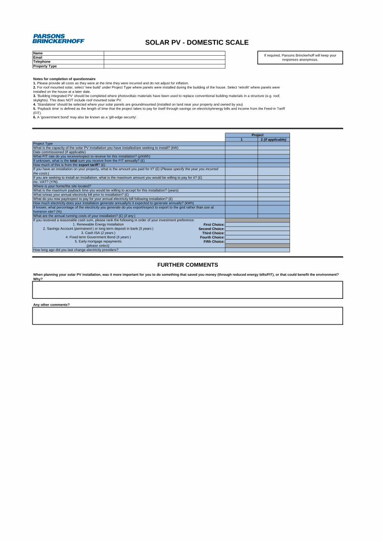
NameEmailTelephoneProperty Type
Notes for completion of questionnaire
1 2 (if applicable)
First Choice:Second Choice:
Third Choice:Fourth Choice:
Fifth Choice:
Any other comments?
If unknown, what is the total sum you receive from the FIT annually? (£)How much of this is from the export tariff? (£)
What is/was your annual electricity bill prior to installation? (£)
If required, Parsons Brinckerhoff will keep your responses anonymous.
What are the annual running costs of your installation? (£) (if any )If you received a reasonable cash sum, please rank the following in order of your investment preference:
Project TypeWhat is the capacity of the solar PV installation you have installed/are seeking to install? (kW)Date commissioned (if applicable)
If you are seeking to install an installation, what is the maximum amount you would be willing to pay for it? (£)
1. Renewable Energy Installation
1. Please provide all costs as they were at the time they were incurred and do not adjust for inflation.2. For roof mounted solar, select 'new build' under Project Type where panels were installed during the building of the house. Select 'retrofit' where panels were installed on the house at a later date.3. 'Building integrated PV' should be completed where photovoltaic materials have been used to replace conventional building materials in a structure (e.g. roof, skylights). This does NOT include roof mounted solar PV.4. 'Standalone' should be selected where your solar panels are groundmounted (installed on land near your property and owned by you)
6. A 'government bond' may also be known as a 'gilt-edge security'.
5. 'Payback time' is defined as the length of time that the project takes to pay for itself through savings on electricity/energy bills and income from the Feed-in Tariff (FIT).
2. Savings Account (permanent ) or long term deposit in bank (5 years )3. Cash ISA (2 years )
4. Fixed term Government Bond (5 years )5. Early mortgage repayments
SOLAR PV - DOMESTIC SCALE
If known, what percentage of the electricity you generate do you export/expect to export to the grid rather than use at home/on site? (%)
If you have an installation on your property, what is the amount you paid for it? (£) (Please specify the year you incurred the costs )
What FIT rate do you receive/expect to receive for this installation? (p/kWh)
inc. VAT? (Y/N)Where is your home/the site located?What is the maximum payback time you would be willing to accept for this installation? (years)
Project
How much electricity does your installation generate annually/is it expected to generate annually? (kWh)What do you now pay/expect to pay for your annual electricity bill following installation? (£)
FURTHER COMMENTSWhen planning your solar PV installation, was it more important for you to do something that saved you money (through reduced energy bills/FIT), or that could benefit the environment? Why?
(please select)How long ago did you last change electricity providers?

URN: 15D/434