https://doi.org/10.3758/s13428-019-01231-3

Parsimonious estimation of signal detection modelsfrom confidence ratings

Ravi Selker1 ·Don van den Bergh1 · Amy H. Criss2 · Eric-Jan Wagenmakers1

© The Author(s) 2019

AbstractSignal detection theory (SDT) is used to quantify people’s ability and bias in discriminating stimuli. The ability to detecta stimulus is often measured through confidence ratings. In SDT models, the use of confidence ratings necessitates theestimation of confidence category thresholds, a requirement that can easily result in models that are overly complex. Asa parsimonious alternative, we propose a threshold SDT model that estimates these category thresholds using only twoparameters. We fit the model to data from Pratte et al. (Journal of Experimental Psychology: Learning, Memory, andCognition, 36, 224–232, 2010) and illustrate its benefits over previous threshold SDT models.

Keywords Signal detection theory · Confidence ratings · Bayesian hierarchical models

Our ability to recognize stimuli allows us to interactsmoothly with the world. We know that if we want to drinkwater it is a good idea to poor it into a cup instead ofonto a piece of paper. We also know that if we want towrite something down it is a good idea to use a pen insteadof a yoga mat. Although recognizing stimuli is sometimesstraightforward, often it is not. Most of the times, ourability to recognize a stimulus is accompanied by a certainamount of noise. When picking mushrooms, it can be hardto distinguish between the mushrooms you can use to topyour beautiful saffron risotto, and the mushrooms that willturn your dinner party into the next Jonestown. Not onlydo eatable and poisonous mushrooms differ in perceptualsimilarity—it is easy to classify a mushroom with a redcap and white spots as poisonous, but difficult to do sofor a poisonous mushroom that looks similar to a commonwhite button mushroom—but the amount of risk involvedin making the wrong decision can also differ betweensituations: when you are starving you might decide to eata suspicious looking mushroom sooner than when you just

� Don van den Berghdonvdbergh@hotmail.com

1 Department of Psychological Methods, University of Amsterdam,Postbus 15906, 1001 NK Amsterdam, The Netherlands

2 Syracuse University, Syracuse, NY, USA

had a full course meal. Signal detection theory (SDT; Tanner& Swets, 1954; Green & Swets, 1966) disentangles theseaspects of recognition by providing different parameters: (1)the amount of information that is available in the stimulus,and (2) the threshold you set for making one or the otherdecision.

In order to separately estimate these two aspects ofrecognition, an SDTmodel needs two pieces of information:(1) the proportion of correctly identified signal stimuli (hitrate, HR; the proportion of poisonous mushrooms that werecorrectly identified as poisonous), and (2) the proportionof incorrectly identified noise stimuli (false alarm rate,FAR; the proportion of non-poisonous mushrooms that wereincorrectly identified as poisonous). Table 1 depicts thefour possible outcomes when discriminating two types ofstimuli; Eqs. 1 and 2 show how these outcomes can beconverted to hit rate and false alarm rate:

Hit Rate = Hits

Hits + Misses, (1)

False Alarm Rate = False Alarms

False Alarms + Correct Rejections. (2)

SDT is a popular model for the analysis of experiments inrecognition memory. The most common experiment in thisfield first requires that participants study a list of words (i.e.,the study list). Following a retention interval, participants

Published online: 8 May 2019

Behavior Research Methods (2019) 51:1953–1967

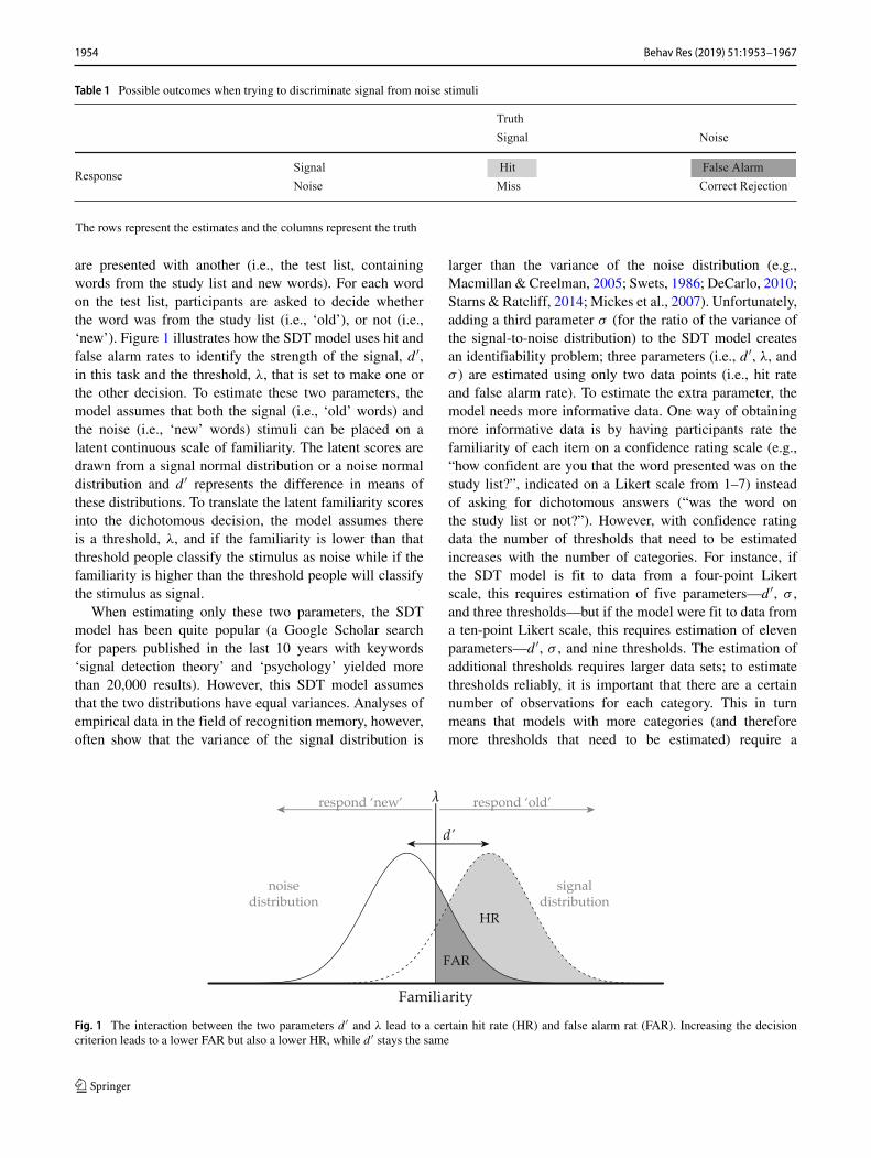
Table 1 Possible outcomes when trying to discriminate signal from noise stimuli

Truth

esioNlangiS

Signal Hit False AlarmResponse

noitcejeRtcerroCssiMesioN

The rows represent the estimates and the columns represent the truth

are presented with another (i.e., the test list, containingwords from the study list and new words). For each wordon the test list, participants are asked to decide whetherthe word was from the study list (i.e., ‘old’), or not (i.e.,‘new’). Figure 1 illustrates how the SDT model uses hit andfalse alarm rates to identify the strength of the signal, d ′,in this task and the threshold, λ, that is set to make one orthe other decision. To estimate these two parameters, themodel assumes that both the signal (i.e., ‘old’ words) andthe noise (i.e., ‘new’ words) stimuli can be placed on alatent continuous scale of familiarity. The latent scores aredrawn from a signal normal distribution or a noise normaldistribution and d ′ represents the difference in means ofthese distributions. To translate the latent familiarity scoresinto the dichotomous decision, the model assumes thereis a threshold, λ, and if the familiarity is lower than thatthreshold people classify the stimulus as noise while if thefamiliarity is higher than the threshold people will classifythe stimulus as signal.

When estimating only these two parameters, the SDTmodel has been quite popular (a Google Scholar searchfor papers published in the last 10 years with keywords‘signal detection theory’ and ‘psychology’ yielded morethan 20,000 results). However, this SDT model assumesthat the two distributions have equal variances. Analyses ofempirical data in the field of recognition memory, however,often show that the variance of the signal distribution is

larger than the variance of the noise distribution (e.g.,Macmillan & Creelman, 2005; Swets, 1986; DeCarlo, 2010;Starns & Ratcliff, 2014; Mickes et al., 2007). Unfortunately,adding a third parameter σ (for the ratio of the variance ofthe signal-to-noise distribution) to the SDT model createsan identifiability problem; three parameters (i.e., d ′, λ, andσ ) are estimated using only two data points (i.e., hit rateand false alarm rate). To estimate the extra parameter, themodel needs more informative data. One way of obtainingmore informative data is by having participants rate thefamiliarity of each item on a confidence rating scale (e.g.,“how confident are you that the word presented was on thestudy list?”, indicated on a Likert scale from 1–7) insteadof asking for dichotomous answers (“was the word onthe study list or not?”). However, with confidence ratingdata the number of thresholds that need to be estimatedincreases with the number of categories. For instance, ifthe SDT model is fit to data from a four-point Likertscale, this requires estimation of five parameters—d ′, σ ,and three thresholds—but if the model were fit to data froma ten-point Likert scale, this requires estimation of elevenparameters—d ′, σ , and nine thresholds. The estimation ofadditional thresholds requires larger data sets; to estimatethresholds reliably, it is important that there are a certainnumber of observations for each category. This in turnmeans that models with more categories (and thereforemore thresholds that need to be estimated) require a

Fig. 1 The interaction between the two parameters d ′ and λ lead to a certain hit rate (HR) and false alarm rat (FAR). Increasing the decisioncriterion leads to a lower FAR but also a lower HR, while d ′ stays the same

1954 Behav Res (2019) 51:1953–1967

larger number of total observations. In recognition memory,accuracy decreases with successive test trials (Criss et al.,2011), limiting the number of observations any individualparticipant can contribute. This problem is compounded ina typical study where multiple conditions, each requiringmany observations, are under investigation simultaneously.Here we introduce a parsimonious method of estimatingthe thresholds by restricting the way the thresholds can beplaced. This parsimony is obtained by modeling thresholdsas a linear transformation of ”unbiased” thresholds, whichonly requires two parameters for any number of thresholds.We estimate parameters in a Bayesian way, and introducea hierarchical extension to our model that allows theestimation of group-level parameters.

The outline of this paper is as follows. First, wewill briefly elaborate on Bayesian methods of parameterestimation. Next, we will introduce our model and theassociated receiver operating characteristics (ROC) curves.We will also show how our model leads to Bayesianestimates of detection measures while taking into accountthe uncertainty of the estimate. Lastly, we will introducethe hierarchical extension and apply the model to memoryrecognition data from Pratte et al. (2010).

Modeling the thresholds

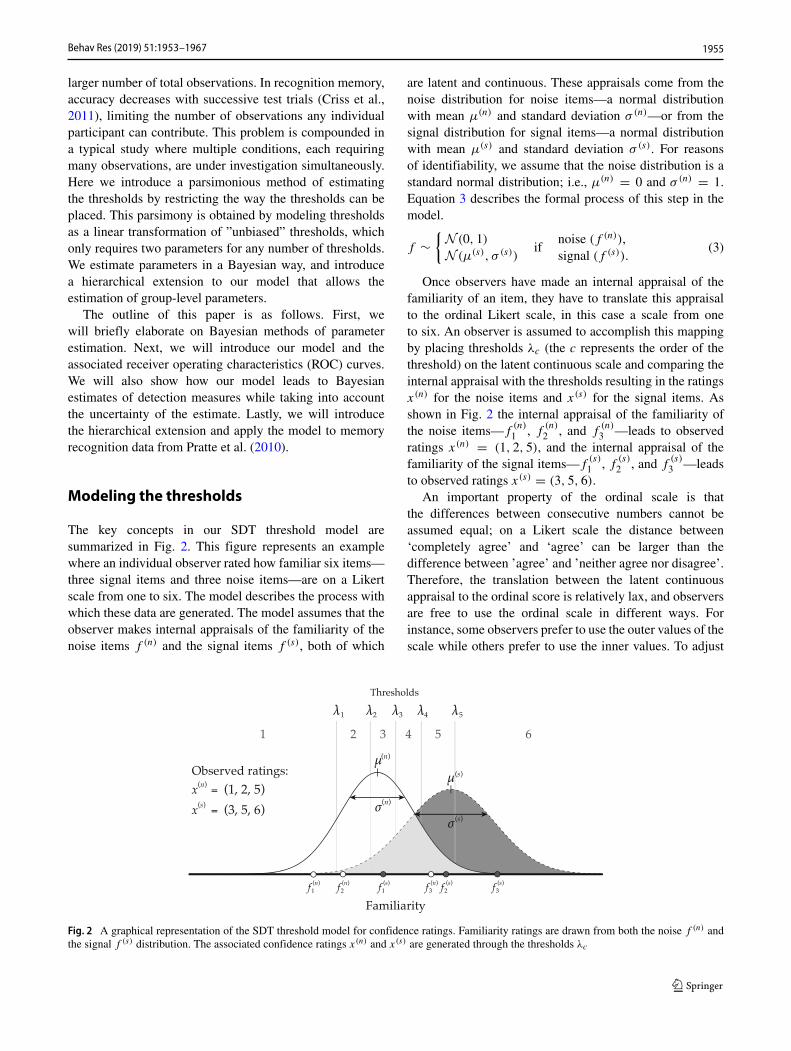
The key concepts in our SDT threshold model aresummarized in Fig. 2. This figure represents an examplewhere an individual observer rated how familiar six items—three signal items and three noise items—are on a Likertscale from one to six. The model describes the process withwhich these data are generated. The model assumes that theobserver makes internal appraisals of the familiarity of thenoise items f (n) and the signal items f (s), both of which

are latent and continuous. These appraisals come from thenoise distribution for noise items—a normal distributionwith mean μ(n) and standard deviation σ (n)—or from thesignal distribution for signal items—a normal distributionwith mean μ(s) and standard deviation σ (s). For reasonsof identifiability, we assume that the noise distribution is astandard normal distribution; i.e., μ(n) = 0 and σ (n) = 1.Equation 3 describes the formal process of this step in themodel.

f ∼{N (0, 1)N (μ(s), σ (s))

ifnoise (f (n)),signal (f (s)).

(3)

Once observers have made an internal appraisal of thefamiliarity of an item, they have to translate this appraisalto the ordinal Likert scale, in this case a scale from oneto six. An observer is assumed to accomplish this mappingby placing thresholds λc (the c represents the order of thethreshold) on the latent continuous scale and comparing theinternal appraisal with the thresholds resulting in the ratingsx(n) for the noise items and x(s) for the signal items. Asshown in Fig. 2 the internal appraisal of the familiarity ofthe noise items—f

(n)1 , f

(n)2 , and f

(n)3 —leads to observed

ratings x(n) = (1, 2, 5), and the internal appraisal of thefamiliarity of the signal items—f

(s)1 , f (s)

2 , and f(s)3 —leads

to observed ratings x(s) = (3, 5, 6).An important property of the ordinal scale is that

the differences between consecutive numbers cannot beassumed equal; on a Likert scale the distance between‘completely agree’ and ‘agree’ can be larger than thedifference between ’agree’ and ’neither agree nor disagree’.Therefore, the translation between the latent continuousappraisal to the ordinal score is relatively lax, and observersare free to use the ordinal scale in different ways. Forinstance, some observers prefer to use the outer values of thescale while others prefer to use the inner values. To adjust

Fig. 2 A graphical representation of the SDT threshold model for confidence ratings. Familiarity ratings are drawn from both the noise f (n) andthe signal f (s) distribution. The associated confidence ratings x(n) and x(s) are generated through the thresholds λc

Behav Res (2019) 51:1953–1967 1955

for these individual differences, a proper model needs to beable to estimate the thresholds that are set by an observerto choose a certain answer. In previous SDT models, thenumber of parameters that needed to be estimated wasdirectly related to the coarseness of the confidence scalethat was used (e.g., Morey et al., 2008). Consequently, thesemodels are not parsimonious and increase in complexityas the Likert scale becomes less coarse. In addition, theprevious approaches are not easily adjusted to incorporateeffect of other functional parameters (e.g., a covariate). Toarrive at a more efficient way of estimating the thresholds,our model is based on a method introduced by Andersand Batchelder (2013) that uses the Linear in Log Oddsfunction. The Linear in Log Odds function requires onlytwo parameters to estimate a potentially large number ofthresholds instead of needing a parameter per threshold (Fox& Tversky, 1995; Gonzalez & Wu, 1999). To estimate C

thresholds, we first assume a best-guess placement of thethresholds. First, we do so on for the interval [0, 1] becauseit is straightforward to place thresholds in an uninformativeway (e.g., the intervals are of equal length). However, sincethe uncertainty in the SDT threshold model is expressedon the interval [−∞, ∞] we next translate the thresholdplacement from the [0, 1] interval to the [−∞, ∞] interval.1

Equation 4 shows how this translation is achieved if wewere to assume that μs = 1 and σ s = 1. Equation 5shows how these ‘unbiased’ thresholds are subsequentlytranslated into the individual ‘biased’ thresholds using alinear transformation.

γc = log

(c/C

1 − c/C

). (4)

λc = aγc + b. (5)

Here, γc is the unbiased threshold for each positionc (e.g., γ1 represents the first unbiased threshold). Scaleparameter a allows the thresholds to be distributed moreclosely to the center of the scale or further away from thecenter of the scale. Shift parameter b allows the thresholdsto focus more on the left or right side of the scale andcould, for example, model response bias. Figure 3 illustrateshow these two parameters can result in different thresholdplacements. Compared to the unbiased thresholds in panela, panel b shows that the thresholds have shifted to the right,and compared to the thresholds in panel b, panel c showsthat the thresholds are placed closer to each other. Comparedto panel c, the thresholds in panel d have shifted more to theright. This shows that two parameters can account for manydifferent ways of threshold placement and can be extendedto any number of thresholds without requiring additionalparameters.

1For the translation we used a logistic quantile function. Other choices,such as a Gaussian quantile function, are also possible.

Note that the outer thresholds are always farther awayfrom their neighboring thresholds than the inner thresholds.At first sight this may look like a major assumption of themodel, but it is not. The probability of observing a certainrating is not related to the distance between thresholds, butrather to the area under the curve (i.e., the integral fromone threshold to the next over either the noise or the signaldistribution).

Bayesian parameter estimation

SDT models have been applied using both classical(Macmillan & Creelman, 2005) and Bayesian frameworks(Rouder & Lu, 2005). In this paper, we adopt the Bayesianframework (Etz et al., 2016; Lee & Wagenmakers, 2013).An important goal of Bayesian statistics is to determine theposterior distribution of the parameters. This distributionexpresses the uncertainty of the parameter estimates afterobserving the data; the more peaked this distributionthe more certain the estimate. To obtain the posteriordistribution of a parameter (e.g., d ′ or λ), the likelihood ismultiplied with the prior distribution, see Eq. 6.

p(θ | data,M)︸ ︷︷ ︸posterior

distribution

proportional to︷︸︸︷∝ p(θ | M)︸ ︷︷ ︸prior

distribution

× p(data | θ,M)︸ ︷︷ ︸likelihood

. (6)

In our case, it is not possible to derive the posteriordistribution analytically and hence we used MCMCsampling techniques (i.e., implemented in JAGS; Plummer,2003) to draw samples from the posterior distribution;with enough samples the approximation to the posteriordistribution becomes arbitrarily close. As priors, we usednormal distributions for all unbounded parameters (meanand shift). For bounded parameters (variances and scale),we used either a gamma prior or a normal distributiontruncated from 0 to ∞. Formal model definitions and priordistributions can be found in the Appendix.

To confirm the performance of the model, we conducteda parameter recovery study. First, we randomly generated100 values for μ(s), σ (s), a, and b2. Each combination ofparameters was used to generate ordinal six-point Likertscale data (240 noise and 240 signal items), after whichthe SDT threshold model was fit to the data. Subsequently,we compared the parameter values used to generate thedata with the means of the posterior distributions of theparameter estimates. The correlations between the data

2The individual values for the parameters were drawn from: μsi ,normal distribution with mean 1 and standard deviation 0.5 truncated at[0, 3], σsi , normal distribution with mean 1 and standard deviation 0.5truncated at [1, 3], a, gamma distribution with shape parameter 2 andrate parameter 2, and b, normal distribution with mean 0 and standarddeviation 0.5.

Behav Res (2019) 51:1953–19671956

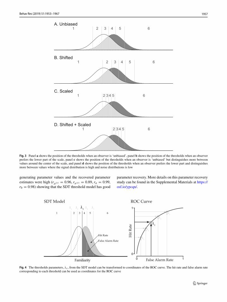
Fig. 3 Panel a shows the position of the thresholds when an observer is ‘unbiased’, panel b shows the position of the thresholds when an observerprefers the lower part of the scale, panel c shows the position of the thresholds when an observer is ‘unbiased’ but distinguishes more betweenvalues around the center of the scale, and panel d shows the position of the thresholds when an observer prefers the lower part and distinguishesmore between values where the signal distribution is high and noise distributions is low

generating parameter values and the recovered parameterestimates were high (rμ(s) = 0.96, rσ (s) = 0.89, ra = 0.99,rb = 0.98) showing that the SDT threshold model has good

parameter recovery. More details on this parameter recoverystudy can be found in the Supplemental Materials at https://osf.io/ypcqn/.

Fig. 4 The thresholds parameters, λc, from the SDT model can be transformed to coordinates of the ROC curve. The hit rate and false alarm ratecorresponding to each threshold can be used as coordinates for the ROC curve

Behav Res (2019) 51:1953–1967 1957

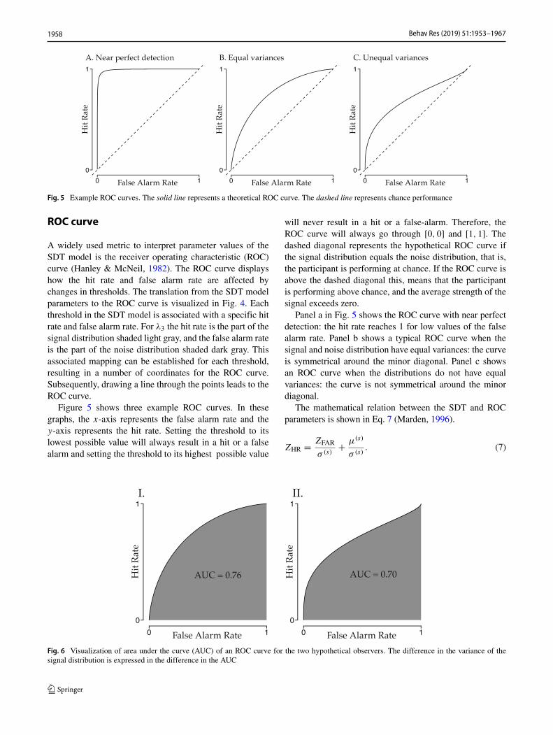
Fig. 5 Example ROC curves. The solid line represents a theoretical ROC curve. The dashed line represents chance performance

ROC curve

A widely used metric to interpret parameter values of theSDT model is the receiver operating characteristic (ROC)curve (Hanley & McNeil, 1982). The ROC curve displayshow the hit rate and false alarm rate are affected bychanges in thresholds. The translation from the SDT modelparameters to the ROC curve is visualized in Fig. 4. Eachthreshold in the SDT model is associated with a specific hitrate and false alarm rate. For λ3 the hit rate is the part of thesignal distribution shaded light gray, and the false alarm rateis the part of the noise distribution shaded dark gray. Thisassociated mapping can be established for each threshold,resulting in a number of coordinates for the ROC curve.Subsequently, drawing a line through the points leads to theROC curve.

Figure 5 shows three example ROC curves. In thesegraphs, the x-axis represents the false alarm rate and they-axis represents the hit rate. Setting the threshold to itslowest possible value will always result in a hit or a falsealarm and setting the threshold to its highest possible value

will never result in a hit or a false-alarm. Therefore, theROC curve will always go through [0, 0] and [1, 1]. Thedashed diagonal represents the hypothetical ROC curve ifthe signal distribution equals the noise distribution, that is,the participant is performing at chance. If the ROC curve isabove the dashed diagonal this, means that the participantis performing above chance, and the average strength of thesignal exceeds zero.

Panel a in Fig. 5 shows the ROC curve with near perfectdetection: the hit rate reaches 1 for low values of the falsealarm rate. Panel b shows a typical ROC curve when thesignal and noise distribution have equal variances: the curveis symmetrical around the minor diagonal. Panel c showsan ROC curve when the distributions do not have equalvariances: the curve is not symmetrical around the minordiagonal.

The mathematical relation between the SDT and ROCparameters is shown in Eq. 7 (Marden, 1996).

ZHR = ZFAR

σ (s)+ μ(s)

σ (s). (7)

Fig. 6 Visualization of area under the curve (AUC) of an ROC curve for the two hypothetical observers. The difference in the variance of thesignal distribution is expressed in the difference in the AUC

Behav Res (2019) 51:1953–19671958

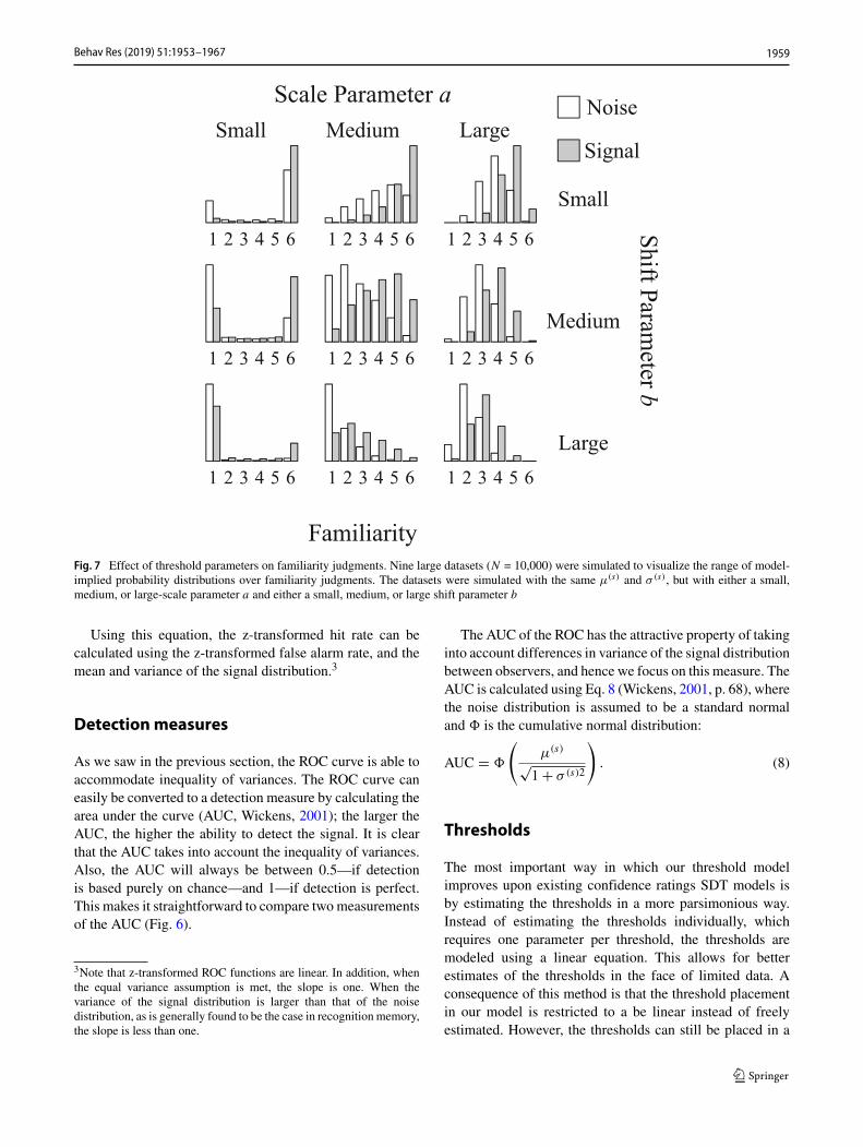
Fig. 7 Effect of threshold parameters on familiarity judgments. Nine large datasets (N = 10,000) were simulated to visualize the range of model-implied probability distributions over familiarity judgments. The datasets were simulated with the same μ(s) and σ (s), but with either a small,medium, or large-scale parameter a and either a small, medium, or large shift parameter b

Using this equation, the z-transformed hit rate can becalculated using the z-transformed false alarm rate, and themean and variance of the signal distribution.3

Detectionmeasures

As we saw in the previous section, the ROC curve is able toaccommodate inequality of variances. The ROC curve caneasily be converted to a detection measure by calculating thearea under the curve (AUC, Wickens, 2001); the larger theAUC, the higher the ability to detect the signal. It is clearthat the AUC takes into account the inequality of variances.Also, the AUC will always be between 0.5—if detectionis based purely on chance—and 1—if detection is perfect.This makes it straightforward to compare twomeasurementsof the AUC (Fig. 6).

3Note that z-transformed ROC functions are linear. In addition, whenthe equal variance assumption is met, the slope is one. When thevariance of the signal distribution is larger than that of the noisedistribution, as is generally found to be the case in recognition memory,the slope is less than one.

The AUC of the ROC has the attractive property of takinginto account differences in variance of the signal distributionbetween observers, and hence we focus on this measure. TheAUC is calculated using Eq. 8 (Wickens, 2001, p. 68), wherethe noise distribution is assumed to be a standard normaland � is the cumulative normal distribution:

AUC = �

(μ(s)

√1 + σ (s)2

). (8)

Thresholds

The most important way in which our threshold modelimproves upon existing confidence ratings SDT models isby estimating the thresholds in a more parsimonious way.Instead of estimating the thresholds individually, whichrequires one parameter per threshold, the thresholds aremodeled using a linear equation. This allows for betterestimates of the thresholds in the face of limited data. Aconsequence of this method is that the threshold placementin our model is restricted to a be linear instead of freelyestimated. However, the thresholds can still be placed in a

Behav Res (2019) 51:1953–1967 1959

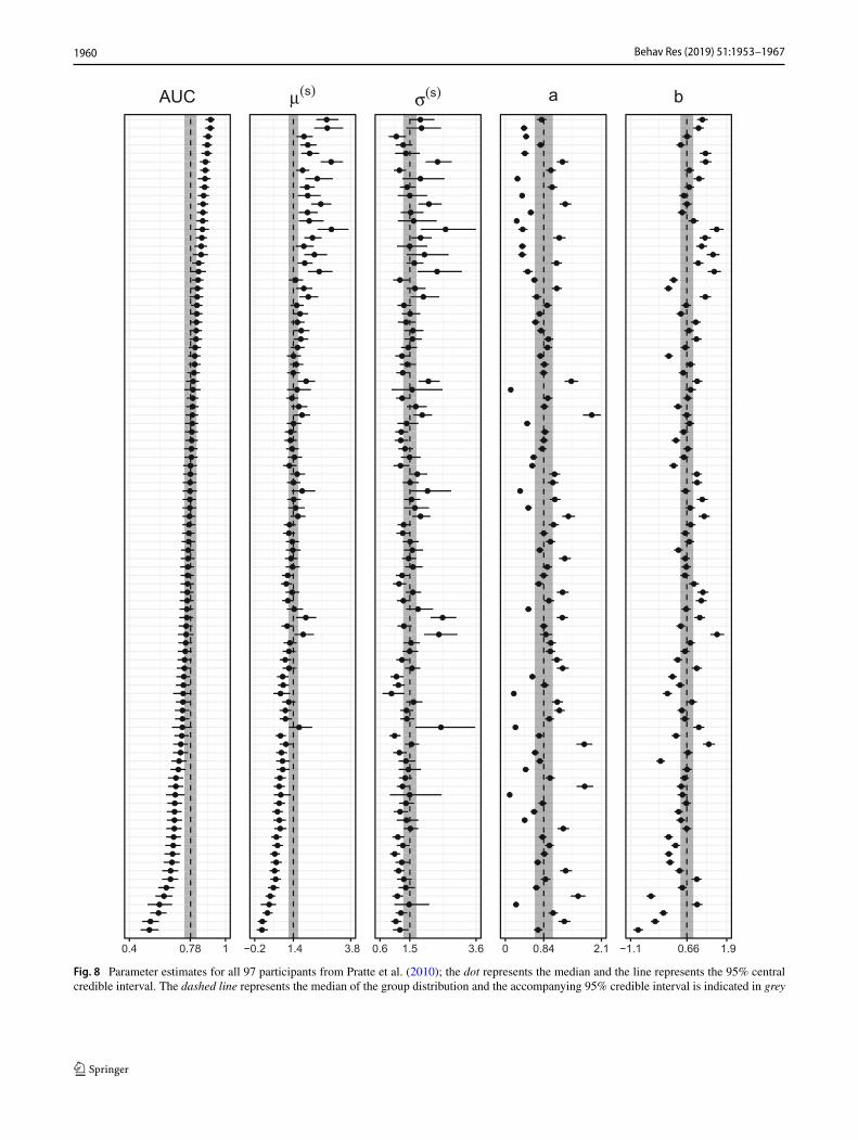
Fig. 8 Parameter estimates for all 97 participants from Pratte et al. (2010); the dot represents the median and the line represents the 95% centralcredible interval. The dashed line represents the median of the group distribution and the accompanying 95% credible interval is indicated in grey

Behav Res (2019) 51:1953–19671960

wide variety of ways. Because the threshold model takesinto account that observers can set their thresholds indifferent ways, similar abilities in signal detection can leadto different data, underscoring the difficulties of drawingconclusions directly from the data. To illustrate this point,we performed a simulation study.

Toobtain plausible values for the simulation study,we firstfitted the threshold SDT model to data from Pratte andRouder (2011), who gathered confidence ratings on a mem-ory recognition task for 97 participants (this data set is des-cribed inmore detail below). Based on the estimated parame-ter values,we chose three values of the scale parameters basedon the 1st , 50th, and 99th percentiles of the estimated values(i.e., a1 = 0.12, a50 = 0.84, a99 = 1.74), and three values ofthe shift parameters based on the 1st , 50th, and 99th per-centiles of the estimated values (i.e., b1=−0.98, b50=0.14,b99=1.10).Weused fixed values ofμ(s) =1 and σ (s) =1 andall possible combinations of the scale and shift parametersto simulate data from the threshold SDT model, resultingin nine different data sets. Figure 7 shows histograms ofthe simulated data. It is clear that the model can describevarious datasets by varying the threshold placement, evenwhen the underlying familiarity distributions are identical.

Figure 7 illustrates that as the scale parameter increases(i.e., moving along the columns from left to right), moreanswers on the inside of the scale are given and as the shiftparameter increases (i.e., moving along the rows from topto bottom), the left side of the scale is used more often. Thiscoverage of possible outcomes makes the model nearly asflexible as having an independent parameter for each thresh-old while minimizing the number of parameters to estimate.

Hierarchical extension

The threshold SDT model can be used to fit data froma single observer. However, often there is interest in thedetection ability of a group of observers, which requiressome sort of aggregation or pooling. One way of pooling isby aggregating the data and then fitting the model on theaggregated data. Another way of pooling is by estimatingthe parameters for each observer individually and then takethe mean or median from these parameter values. Althoughthese methods are computationally simple, they lack aformal model that describes how the group level distributionrelates to individual parameter values.

In contrast, in theBayesianhierarchical approach, individ-ual subject parameters are drawn from a group distribution(Gelman & Hill, 2006). Because the subjects are modeledas part of a group, the individual parameters shrink towardsthe group mean (Efron & Morris, 1977). The benefit ofshrinkage is that the model is much more resistant to over-fitting, as the group-level information makes the individual

estimates less susceptible to noise fluctuations (Shiffrinet al., 2008). In the hierarchical threshold model, we intro-duce group distributions for the mean and variance of thesignal distribution, and for the scale and shift parameters ofthe thresholds. The priors for unbounded parameters (meanand shift) are normal distributions whereas the priors forbounded parameters (variance and scale) are either gammadistributions or truncated normal distributions. Exact modelspecifications and priors are shown in the Appendix4.

To confirm the performance of the model we conducted aparameter recovery study. The formal model definitionsincluding prior distributions can be found in the Appendix.First, we fitted the hierarchical SDT threshold model to thedata of Pratte et al. (2010) (see next section for a more elab-orate explanation).We used themeans of the posterior distri-butions for the individual level parameters μ(s), σ (s), a, andb to generate plausible data.Next, we fit themodel to the syn-thetic data and drew posterior samples from the hierarchicalSDT threshold model. Subsequently, we compared the data-generating parameter values to the means of the posteriordistributions for the parameter estimates. The correlationbetween the data-generating parameter values and the recov-ered parameter estimates was high (rμ(s) =0.96, rσ (s) =0.90,ra = 0.99, rb = 0.99, see Fig. 15) showing that the hierar-chical SDT threshold model has good parameter recovery.More details on this parameter recovery study can be foundin the Supplemental Materials at https://osf.io/ypcqn/. Thenext section applies the model to experimental data.

Application to experimental data

We fitted the hierarchical SDT threshold model to data fromPratte et al. (2010) who had gathered confidence ratingson a memory recognition task from 97 participants. Eachparticipant studied 240 words—each word for 1850 mswith 250-ms blank periods between two words—randomlyselected from a set of 480 words. After the study phase,participants had to indicate how confident they were that aword was part of the study list on a six-point Likert scale(using the ratings “sure new”, “believe new”, “guess new”,“guess studied”, “believe studied”, and “sure studied”) forthe whole batch of 480 words. In this experiment, the wordsin the study list represent the signal items, while the wordsthat were not in the study list represent the noise items.

Figure 8 shows the estimated median and 95% credibleintervals for each parameter in themodel. The dashed vertical

4We opted not to use highly uninformative priors as the resultingprior ROC curves are implausible. See Figs. 13 and 14 for theprior and posterior ROC curves under slightly informed and highlyuninformative priors. Different priors had negligible effect on theposterior distribution, see the Supplemental Materials Figures onhttps://osf.io/ypcqn/ for a comparison.

Behav Res (2019) 51:1953–1967 1961

line represents the median of the group level estimation withthe 95% credible interval shaded gray. The parameters areestimatedwith agoodprecision; in general, the credible inter-vals are narrow.We investigated the fit of the thresholdmodelto the data from Pratte using posterior predictive checks.Although there is some misfit for lower proportions, themodel appears to describe the data adequately, see Fig. 16.

The model parameters can also be used to produce an ROCcurve. Figure 9 shows theROCcurve for the group level, wherethe shaded area represents the uncertainty in the estimate,and the density plot shows the posterior distribution for theAUC. Note that the uncertainty in the ROC and the AUC isinduced by the uncertainty in the model parameters.

Discussion

The threshold SDT model describes how people estimate thefamiliarity of signal and noise items. The main contributionof the model is that it provides a parsimonious way of estimat-ing the thresholds instead of sacrificing one parameter perthreshold. We also showed how this model can be applied toexperimental data. This paper presents a first effort in par-simonious threshold estimation that should be applicable tomany SDT applications. It can also be used as a startingpoint for more complicated applications of SDT models. Astraightforward empirical test of the threshold SDT modelis to examine how experimental manipulations map onto themodel parameters. For example, one may conduct a test ofspecific influence and examine the extent to which effectsof changes in base-rate are absorbed by the threshold a andb parameters.

Because the threshold SDT model features only fourparameters, it is relatively straightforward to add other

Fig. 9 Group level ROC curve with the 95% credible interval in greyand the area under the curve (AUC) with the uncertainty in the estimateexpressed through the posterior distribution

effects, e.g., the item effects mentioned in the discussion ofPratte and Rouder (2011). For example, a researcher couldhypothesize that there is a difference in responsebias betweentwo conditions, and that this difference maps onto the shiftparameter. To incorporate this into the model, Eq. 5 couldbe modified to include a covariate on the shift of the thresh-olds. Such a modification is identical to adding a predictorto a regression model. This allows for relatively easy groupcomparisons; in contrast, such comparisons are difficultfor models that require one parameter per threshold, asmultiple estimates need to be considered simultaneously.

Expanding the transformation of the thresholds into alinear model introduces the need for model comparison. Toassess the relevance of a predictor, one compares a modelwithout the predictor to a model with the predictor. Withinthe Bayesian framework, comparing models is often doneby means of Bayes factors (Mulder & Wagenmakers, 2016;Jeffreys, 1961). Although no analytical formulas exist forcalculating Bayes factor for SDT models, an approximationcan be obtained using numerical techniques on the obtainedMCMC samples, e.g., via bridge sampling Gronau et al.(2017) and Meng and Wong (1996).

In sum, the threshold SDT model provides a parsimo-nious and straightforward account of confidence rating data,allowing researchers to quantify not only discriminabilitybut also confidence category thresholds. The uncertaintyin the model’s parameter estimates can be used to induceuncertainty in crucial SDT measures such as the area underthe ROC curve.

Acknowledgements This research was funded by a research talentgrant from NWO (Dutch Organization for Scientific Research)awarded to Ravi Selker. Supplemental Materials (including all thescripts and data needed to reproduce the analyses in this paper) can befound on https://osf.io/ypcqn/.

Open Access This article is distributed under the terms of theCreative Commons Attribution 4.0 International License (http://creativecommons.org/licenses/by/4.0/), which permits unrestricteduse, distribution, and reproduction in any medium, provided you giveappropriate credit to the original author(s) and the source, provide alink to the Creative Commons license, and indicate if changes weremade.

Appendix

This Appendix contains both the formal BUGS modeldefinition and the graphical representation of the SDTthreshold model and the hierarchical SDT threshold model.The R code that calls the BUGS code is available athttps://osf.io/v3b76/. The model definition and graphicalrepresentation define all priors and relations betweenparameters and data. For more information on the BUGSmodeling language and the graphical representation of thesemodels, see Lee and Wagenmakers (2013).

Behav Res (2019) 51:1953–19671962

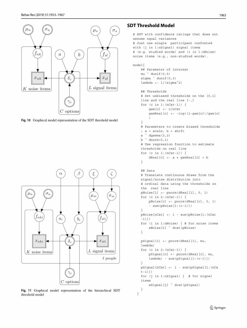
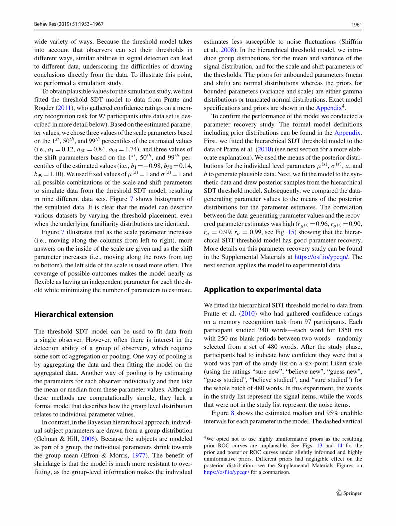
Fig. 10 Graphical model representation of the SDT threshold model

Fig. 11 Graphical model representation of the hierarchical SDTthreshold model

SDT ThresholdModel

Behav Res (2019) 51:1953–1967 1963

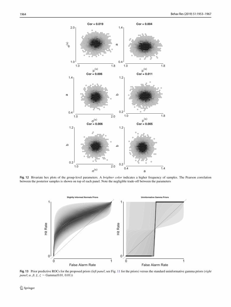
Fig. 12 Bivariate hex plots of the group-level parameters. A brighter color indicates a higher frequency of samples. The Pearson correlationbetween the posterior samples is shown on top of each panel. Note the negligible trade-off between the parameters

Fig. 13 Prior predictive ROCs for the proposed priors (left panel; see Fig. 11 for the priors) versus the standard uninformative gamma priors (rightpanel; α, β, ξ, ζ ∼ Gamma(0.01, 0.01))

Behav Res (2019) 51:1953–19671964

Fig. 14 Posterior predictive ROCs for the proposed priors (left panel; see Fig. 11 for the priors) versus the standard uninformative gamma priors(right panel; α, β, ξ, ζ ∼ Gamma(0.001, 0.001))

Fig. 15 Parameter retrieval of the group level parameters of thesimulation study with the hierarchical model

Fig. 16 Posterior predictive check for the data from Pratte et al.(2010). Observed proportions of a rating per person (x-axis) versusposterior predictive means of the model (y-axis). The model fits ratingswith a higher observed proportion better than those with a lowerobserved proportion. This occurs because those ratings constitutemore observations and are weighed more by the likelihood. Lowerproportions are captured less well by the model. Likewise, the lowerproportions are based on less data and are therefore more noisy

Behav Res (2019) 51:1953–1967 1965

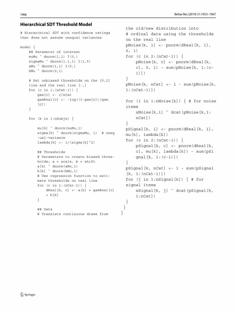
Hierarchical SDT ThresholdModel

Behav Res (2019) 51:1953–19671966

References

Anders, R., & Batchelder, W. (2013). Cultural consensus theory for theordinal data case. Psychometrika, 80, 151–181.

Criss, A. H., Malmberg, K. J., & Shiffrin, R. M. (2011). Outputinterference in recognition memory. Journal of Memory andLanguage, 64(4), 316–326.

DeCarlo, L. (2010). On the statistical and theoretical basis of signal detec-tion theory and extensions: Unequal variance, random coefficient,and mixture models. Journal of Mathematical Psychology, 54,304–313.

Efron, B., & Morris, C. (1977). Stein’s paradox in statistics. ScientificAmerican, 236, 119–127.

Etz, A., Gronau, Q. F., Dablander, F., Edelsbrunner, P., & Baribault,B. (2016). How to become a Bayesian in eight easy steps: Anannotated reading list.

Fox, C. R., & Tversky, A. (1995). Ambiguity aversion andcomparative ignorance. The Quarterly Journal of Economics,110(3), 585–603.

Gelman, A., & Hill, J. (2006). Data analysis using regression andmultilevel/hierarchical models. Cambridge: Cambridge UniversityPress.

Gonzalez, R., & Wu, G. (1999). On the shape of the probabilityweighting function. Cognitive Psychology, 38(1), 129–166.

Green, D. M., & Swets, J. (1966). Signal detection theory andpsychophysics. Wiley: New York.

Gronau, Q. F., Sarafoglou, A., Matzke, D., Ly, A., Boehm, U.,Marsman, M., & Steingroever, H. (2017). A tutorial on bridgesampling. arXiv:1703.05984

Hanley, J. A., & McNeil, B. (1982). The meaning and use of the areaunder a receiver operating characteristic (ROC) curve. Radiology,143, 29–36.

Jeffreys, H. (1961). Theory of probability. Oxford: Oxford UniversityPress.

Lee, M. D., & Wagenmakers, E. J. (2013). Bayesian modeling forcognitive science: A practical course. Cambridge: CambridgeUniversity Press.

Macmillan, N. A., & Creelman, C. (2005). Detection theory: A user’sguide Mahwah. NJ: Lawrence Erlbaum.

Marden, J. I. (1996). Analyzing and modeling rank data. Boca Raton:CRC Press.

Meng, X. L., & Wong, W. H. (1996). Simulating ratios of normalizingconstants via a simple identity: atheoretical exploration. StatisticaSinica, 6, 831–860.

Mickes, L., Wixted, J. T., & Wais, P. (2007). A direct test of theunequal-variance signal detection model of recognition memory.Psychonomic Bulletin & Review, 14(5), 858–865.

Morey, R. D., Pratte, M. S., & Rouder, J. (2008). Problematiceffects of aggregation in zROC analysis and a hierarchicalmodeling solution. Journal of Mathematical Psychology, 52, 376–388.

Mulder, J., & Wagenmakers, E. J. (2016). Editors’ introduction to thespecial issue ”Bayes factors for testing hypotheses in psychologi-cal research: Practical relevance and new developments”. Journalof Mathematical Psychology, 72, 1–5.

Plummer, M. (2003). Jags: A program for analysis of Bayesiangraphical models using Gibbs sampling. In Hornik, K., Leisch,F., & Zeileis, A. (Eds.) Proceedings of the 3rd internationalworkshop on distributed statistical computing (DSC 2003),(pp. 20–22).

Pratte, M. S., Rouder, J. N., &Morey, R. (2010). Separating mnemonicprocess from participant and item effects in the assessment of ROCasymmetries. Journal of Experimental Psychology: Learning,Memory, and Cognition, 36, 224–232.

Pratte, M. S., & Rouder, J. (2011). Hierarchical single-and dual-process models of recognition memory. Journal of MathematicalPsychology, 55, 36–46.

Rouder, J. N., & Lu, J. (2005). An introduction to Bayesianhierarchical models with an application in the theory of signaldetection. Psychonomic Bulletin & Review, 12, 573–604.

Shiffrin, R. M., Lee, M. D., Kim, W., & Wagenmakers, E. J. (2008).A survey of model evaluation approaches with a tutorial on hierarchi-cal Bayesian methods. Cognitive Science, 32, 1248–1284.

Starns, J. J., & Ratcliff, R. (2014). Validating the unequal-variance assumption in recognition memory using responsetime distributions instead of ROC functions: A diffusion modelanalysis. Journal of Memory and Language, 70, 36–52.

Swets, J. (1986). Form of empirical ROCs indiscrimination anddiagnostic tasks: Implications for theory and measurement ofperformance. Psychological Bulletin, 99, 181–198.

Tanner, Jr., W. P., & Swets, J. (1954). A decision-making theory ofvisual detection. Psychological Review, 61, 401–409.

Wickens, T. (2001). Elementary signal detection theory. New York:Oxford University Press.

Publisher’s note Springer Nature remains neutral with regard tojurisdictional claims in published maps and institutional affiliations.

Behav Res (2019) 51:1953–1967 1967