Parity-constrained Triangulations with Steiner points

Victor Alvarez∗

October 31, 2012

Abstract

Let P ⊂ R2 be a set of n points, of which k lie in the interior of the convex

hull CH(P) of P . Let us call a triangulation T of P even (odd) if and only if allits vertices have even (odd) degree, and pseudo-even (pseudo-odd) if at least the k

interior vertices have even (odd) degree. On the one hand, triangulations havingall its interior vertices of even degree have one nice property; their vertices can be3-colored, see [1, 2, 3]. On the other hand, odd triangulations have recently found anapplication in the colored version of the classic “Happy Ending Problem” of Erdosand Szekeres, see [4].

In this paper we show that there are sets of points that admit neither pseudo-even nor pseudo-odd triangulations. Nevertheless, we show how to construct a set ofSteiner points S = S(P ) of size at most k

3+c, where c is a positive constant, such that

a pseudo-even (pseudo-odd) triangulation can be constructed on P ∪ S. Moreover,we also show that even (odd) triangulations can always be constructed using at mostn

3+ c Steiner points, where again c is a positive constant. Our constructions have

the property that every Steiner point lies in the interior of CH(P ).

1 Introduction

Let P ⊂ R2 be a set of n points in general position and let Γ : P → {0, 1} be an

assignment of parities to the elements of P , where 0 means even and 1 means odd. LetG be a straight-edge plane graph with vertex set P . We say that a vertex v ∈ P of G ishappy, with respect to G, if and only if the degree of v in G is of the parity assigned tov by Γ. If a vertex is not happy w.r.t. G we will say that v is unhappy. If the graph G isclear from context we will just say that vertices are happy or unhappy without referringto G.

Given P and Γ, the problem of finding plane graphs on P that maximize the numberof happy vertices has recently received some attention. In [5] it was shown that onecan always construct a tree, a 2-connected outerplanar graph, and a pointed pseudo-triangulation that makes all but at most three vertices happy. For the class of triangu-lations it was shown that one can always construct one that makes essentially 2n

3of its

∗Fachrichtung Informatik, Universitat des Saarlandes, alvarez@cs.uni-saarland.de.

1

vertices happy, but a configuration of points with parities was also shown where at leastn108

vertices remain unhappy regardless of the chosen triangulation. The constructionof this lower bound requires the use of both parities, but the authors pointed out thatthere are two particular cases that might accept triangulations with as many as n−o(n)happy vertices. These two particular cases are the ones where the parities assigned tothe elements of P by Γ are either all even or all odd respectively. However, showingthat in those particular cases n − o(n) vertices can be made happy turned out to bevery challenging. In the same paper the authors showed that in the all-even case, a tri-angulation that makes at least 2n

3vertices happy can always be constructed. They also

showed that in the all-odd case a 10

13fraction of happy vertices can always be ensured.

These two special cases, all even or all odd, are of significant interest since theyhave interesting properties and/or applications. For example, it is well known that aconnected graph G having all its vertices of even degree is Eulerian. If on top of it G

happens to be a triangulation as well, then G is also 3-colorable, see [1, 2] for a generalreference on 3-colorable planar graphs. Those two properties are usually considered“nice” in a graph, and they are characterized only by the parity of the degree of itsvertices. For 3-colorability of triangulations a slightly weaker characterization is known:T is a triangulation having all its interior vertices of even degree if and only if T is3-colorable, see [3] for example. The application related to the all-odd case is a little bitmore intricate and we refer the reader to [4] where this application is shown.

Let P be as before. We will say that a triangulation T of P is even, or odd, if and onlyif the degree of every vertex of T is even, or odd respectively. If only the interior verticesof T are even, or odd, we will say that T is pseudo-even, or pseudo-odd respectively.This defines four kinds of triangulations of P : Even, pseudo-even, odd, pseudo-odd.

In this paper we attack the following problem: Given P and one kind T of triangula-tions of the four mentioned above, construct a set S = S(P,T ) such that a triangulationof kind T can always be constructed on P ∪ S.

Thus, the problem attacked in this paper can be seen as the Steiner-point version ofthe ones regarding triangulations presented in [5]. With this idea in mind, the followinglemma is worth noting:

Lemma 1. There are arbitrarily large sets of points that, without the use of Steiner

points, admit neither pseudo-even nor pseudo-odd triangulations.

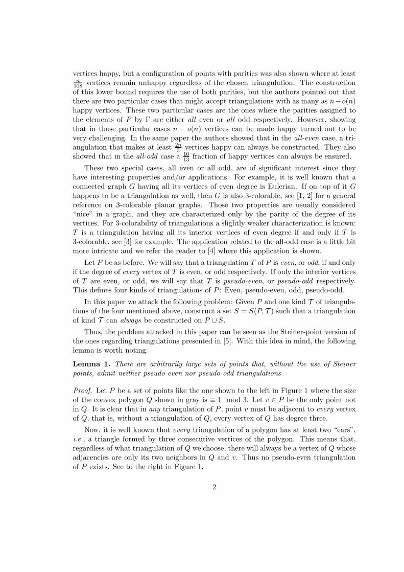
Proof. Let P be a set of points like the one shown to the left in Figure 1 where the sizeof the convex polygon Q shown in gray is ≡ 1 mod 3. Let v ∈ P be the only point notin Q. It is clear that in any triangulation of P , point v must be adjacent to every vertexof Q, that is, without a triangulation of Q, every vertex of Q has degree three.

Now, it is well known that every triangulation of a polygon has at least two “ears”,i.e., a triangle formed by three consecutive vertices of the polygon. This means that,regardless of what triangulation of Q we choose, there will always be a vertex of Q whoseadjacencies are only its two neighbors in Q and v. Thus no pseudo-even triangulationof P exists. See to the right in Figure 1.

2

v

Q

v

u w u w

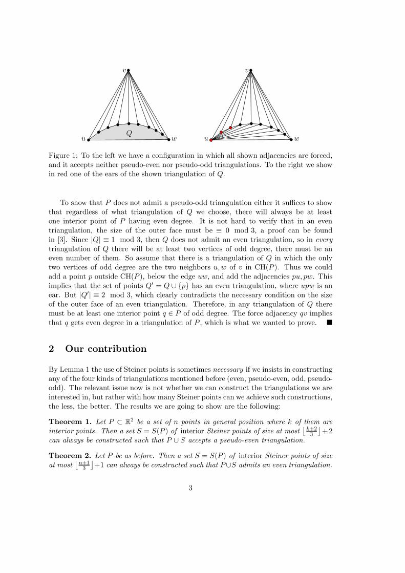
Figure 1: To the left we have a configuration in which all shown adjacencies are forced,and it accepts neither pseudo-even nor pseudo-odd triangulations. To the right we showin red one of the ears of the shown triangulation of Q.

To show that P does not admit a pseudo-odd triangulation either it suffices to showthat regardless of what triangulation of Q we choose, there will always be at leastone interior point of P having even degree. It is not hard to verify that in an eventriangulation, the size of the outer face must be ≡ 0 mod 3, a proof can be foundin [3]. Since |Q| ≡ 1 mod 3, then Q does not admit an even triangulation, so in every

triangulation of Q there will be at least two vertices of odd degree, there must be aneven number of them. So assume that there is a triangulation of Q in which the onlytwo vertices of odd degree are the two neighbors u,w of v in CH(P ). Thus we couldadd a point p outside CH(P ), below the edge uw, and add the adjacencies pu, pw. Thisimplies that the set of points Q′ = Q ∪ {p} has an even triangulation, where upw is anear. But |Q′| ≡ 2 mod 3, which clearly contradicts the necessary condition on the sizeof the outer face of an even triangulation. Therefore, in any triangulation of Q theremust be at least one interior point q ∈ P of odd degree. The force adjacency qv impliesthat q gets even degree in a triangulation of P , which is what we wanted to prove. �

2 Our contribution

By Lemma 1 the use of Steiner points is sometimes necessary if we insists in constructingany of the four kinds of triangulations mentioned before (even, pseudo-even, odd, pseudo-odd). The relevant issue now is not whether we can construct the triangulations we areinterested in, but rather with how many Steiner points can we achieve such constructions,the less, the better. The results we are going to show are the following:

Theorem 1. Let P ⊂ R2 be a set of n points in general position where k of them are

interior points. Then a set S = S(P ) of interior Steiner points of size at most⌊

k+2

3

⌋

+2can always be constructed such that P ∪ S accepts a pseudo-even triangulation.

Theorem 2. Let P be as before. Then a set S = S(P ) of interior Steiner points of size

at most⌊

n+1

3

⌋

+1 can always be constructed such that P∪S admits an even triangulation.

3

Theorem 3. Let P ⊂ R2 be a set of n points in general position where k of them are

interior points. Then a set S = S(P ) of interior Steiner points of size at most⌊

k3

⌋

+ c,

with c a positive constant, can always be constructed such that P ∪S accepts a pseudo-odd

triangulation.

Theorem 4. Let P be as before. Then a set S = S(P ) of interior Steiner points of size

at most⌊

n−1

3

⌋

+ c, with c a positive constant, can always be constructed such that P ∪S

admits an odd triangulation.

The proofs of all theorems will be constructive. The rest of the paper is dividedas follows: In Section 3 we start with some preliminaries. In Section 4 and 5 we showalgorithms that imply Theorems 1, 2, and Theorems 3, 4 respectively. We close thepaper in Section 6 we some observations and conclusions.

3 Pre-processing of P

Let us quickly recall that given a polygon P, a vertex v of P is called reflex if the internalangle at v is larger than π. We will call it convex otherwise. Also, by a suitable rotationof P we can assume that the vertex v of CH(P ) with the lowest y-coordinate is unique.

The following pre-processing of P will be done: Using v as a pivot we will sort eachinterior point of P by its angle with respect to v. Let p1, . . . , pk, be a labeling, from leftto right with respect to this angular order, of the interior points of P . Let p0, pk+1 bethe left and right neighbors of v on CH(P ) respectively.

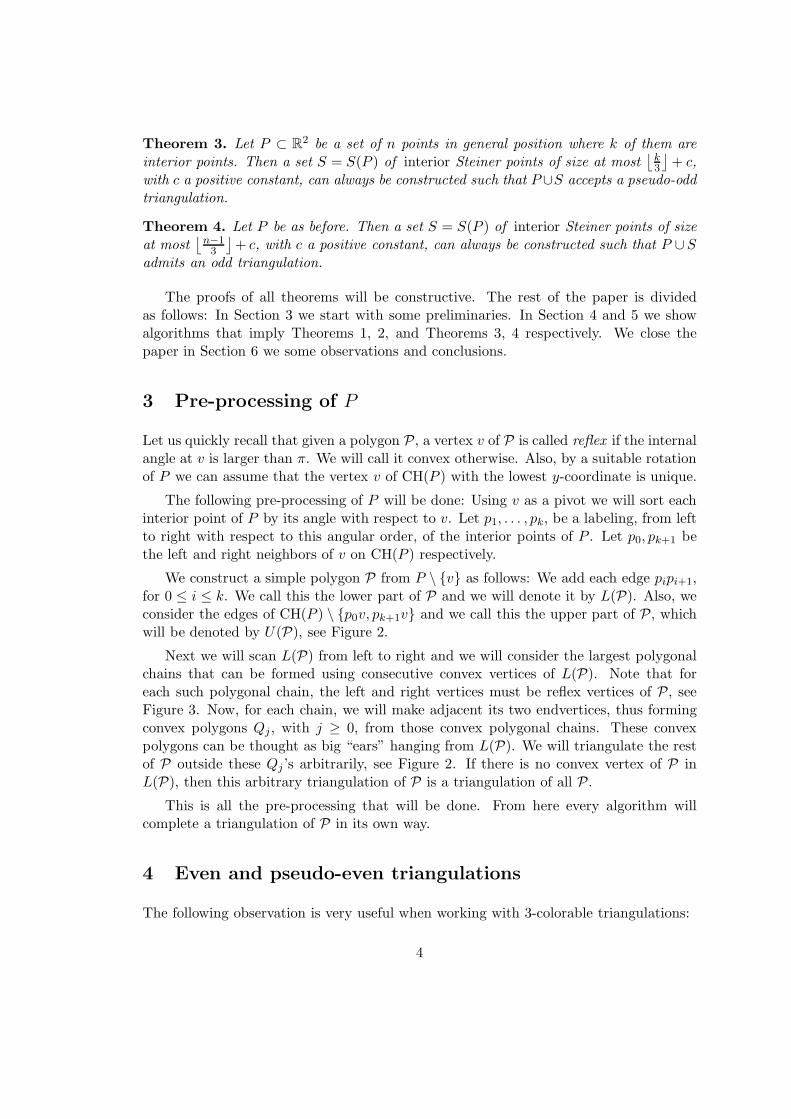
We construct a simple polygon P from P \ {v} as follows: We add each edge pipi+1,for 0 ≤ i ≤ k. We call this the lower part of P and we will denote it by L(P). Also, weconsider the edges of CH(P ) \ {p0v, pk+1v} and we call this the upper part of P, whichwill be denoted by U(P), see Figure 2.

Next we will scan L(P) from left to right and we will consider the largest polygonalchains that can be formed using consecutive convex vertices of L(P). Note that foreach such polygonal chain, the left and right vertices must be reflex vertices of P, seeFigure 3. Now, for each chain, we will make adjacent its two endvertices, thus formingconvex polygons Qj , with j ≥ 0, from those convex polygonal chains. These convexpolygons can be thought as big “ears” hanging from L(P). We will triangulate the restof P outside these Qj ’s arbitrarily, see Figure 2. If there is no convex vertex of P inL(P), then this arbitrary triangulation of P is a triangulation of all P.

This is all the pre-processing that will be done. From here every algorithm willcomplete a triangulation of P in its own way.

4 Even and pseudo-even triangulations

The following observation is very useful when working with 3-colorable triangulations:

4

vp0 pk+1

vp0 pk+1

Figure 2: To the left we have the polygon P on n − 1 vertices in gray. The convexpolygons formed by scanning L(P) from left to right are shown dashed. Note that eachpair of consecutive convex polygons shares at most one vertex. To the right we see atriangulation T (P) of P. The dashed edges are the only ones that are not arbitrary.

Observation 1. Let T be a 3-colored triangulation with outer face C, not necessarily

convex, and let u, v, w be three consecutive vertices of C. If the degree of v in T is even,

then the color of u is different than the color of w. If the degree of v in T is odd, then

both u,w have the same color.

We can now continue with the algorithm. Let us triangulate each Qj, if any exists, asfollows: Take its vertex with the lowest y-coordinate, breaking ties arbitrarily, and join itwith straight-line segments to all other vertices of Qj, in case that Qj has more than threevertices. This is usually called a “fan” triangulation. These fan triangulations along thearbitrary triangulation outside the Qj ’s complete a triangulation T (P) of polygon P.

It is well-known that triangulation T (P) can be 3-colored, see [6], thus we will doit, and observe that the only colorless vertex is v, the one we used in the beginning tosort P angularly. Clearly, if a triangulation of P is 3-colorable, then it must be at least

pseudo-even, thus our idea now is to complete a 3-colorable triangulation of P usingT (P) and its 3-coloring. So at all time we will use a 3-coloring as a measure of thecorrectness of our algorithm.

From this point on, our construction is done by case analysis. We will assumewithout loss of generality that the colors at our disposal are {0, 1, 2}. Note that as T (P)is already 3-colored, if all the interior vertices of P are colored by only two colors, say0, 1, we could use color 2 for v without violating the 3-coloring of T (P), and hence,using the straight-line segments that connect v with each vertex of L(P), we obtain a3-colorable triangulation of P . Nevertheless, in general it is not going to happen thatthe interior vertices can be colored using only two colors, hence we need to do somethingelse in such cases. We will proceed in a line-sweep fashion from p0 to pk+1 with respectto the angular order around v.

5

Let us fix the color of v as the color of the smallest chromatic class in L(P) using the3-coloring of T (P), and say that color is i1 without loss of generality, 0 ≤ i ≤ 2. Notethat the points in L(P) with color i are the ones causing trouble to complete the desiredtriangulation, hence we will handle those points depending on their kind in P, namely ifthey are reflex or convex vertices of P. We will keep the invariant that, by the time weare processing an interior point pj, edge vpj is present, and all interior points pr, withr < j, have even degree already, except possibly for p0. Also note that by this time, ifthe degree of pj is odd it is because pj+1 has color i, due to Observation 1.

Let us start now with our case analysis, we will assume that we are currently process-ing the interior point pj , 1 ≤ j < k, so again, we will assume that the edge vpj is alreadypresent in the partial triangulation of P constructed so far. We have the following cases:

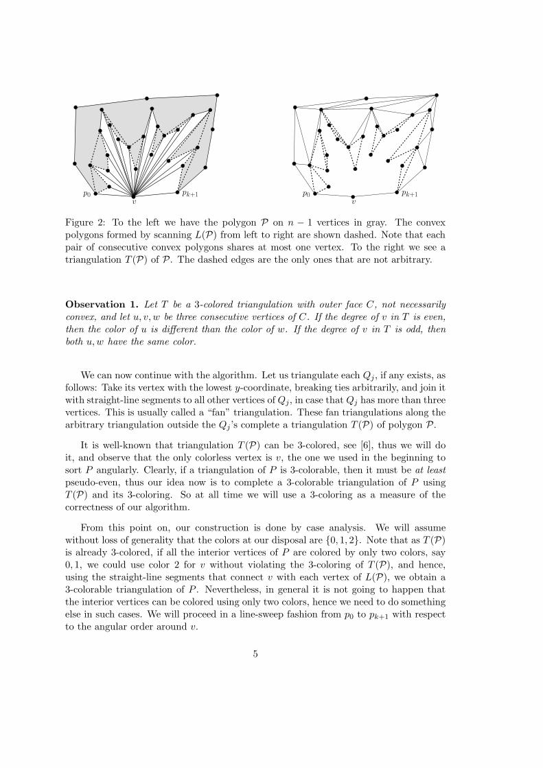
() Point pj+1 is of color i, just as v, and is a reflex vertex of P. If points pj andpj+2 are of different color then we can just add the edge pjpj+2, since pj+1 hasalready even degree in T (P), see to the left in Figure 3. Thus we can add the edgevpj+2 and move to pj+2. If on the other hand, pj and pj+2 have the same color,we introduce one Steiner point s, below L(P), of the third color different than theone of pj and v, which will be adjacent to pj , pj+1, pj+2 and v, as shown in themiddle in Figure 3. Thus we can again move to pj+2 and continue.

v

pj+1pj+2

pj

pj+1

pj

pj+2

pl

Q

v

pj+1pj+2

s

pj

v

pj+1

pj+2

s

pj

Figure 3: The point pj is currently being processed. Point pj+1 is of the same color i ofv. If pj and pj+2 have the same color, then one Steiner point suffices to be able to moveto pj+2. To the right the convex polygon Q is shown in gray. Point pj+1 is the pivot ofthe fan triangulation of Q.

() Point pj+1 is of color i again but a convex vertex of P. If pj and pj+2 have thesame color we proceed just as before, introducing one Steiner point s, below L(P)and of the third available color, which will be again adjacent to pj, pj+1, pj+2 andv. We move to pj+2 and continue, see in the middle in Figure 3.

1In the figures, unless otherwise stated, we will use colors {i, i + 1, i + 2} = {black, red,blue}, witharithmetic modulo 3.

6

So let us assume that pj and pj+2 have different colors, say w.l.o.g. i + 1 andi + 2 respectively. Note that, as pj+1 is a convex vertex of P, it must be partof one of the convex polygons Q1, . . . Qr, the big “ears”, we constructed in thepre-processing phase. Let us denote this one convex polygon simply by Q, and itsrightmost vertex by pl, l ≥ j + 2, according to the angular order around v.

We have now the following sub-cases:

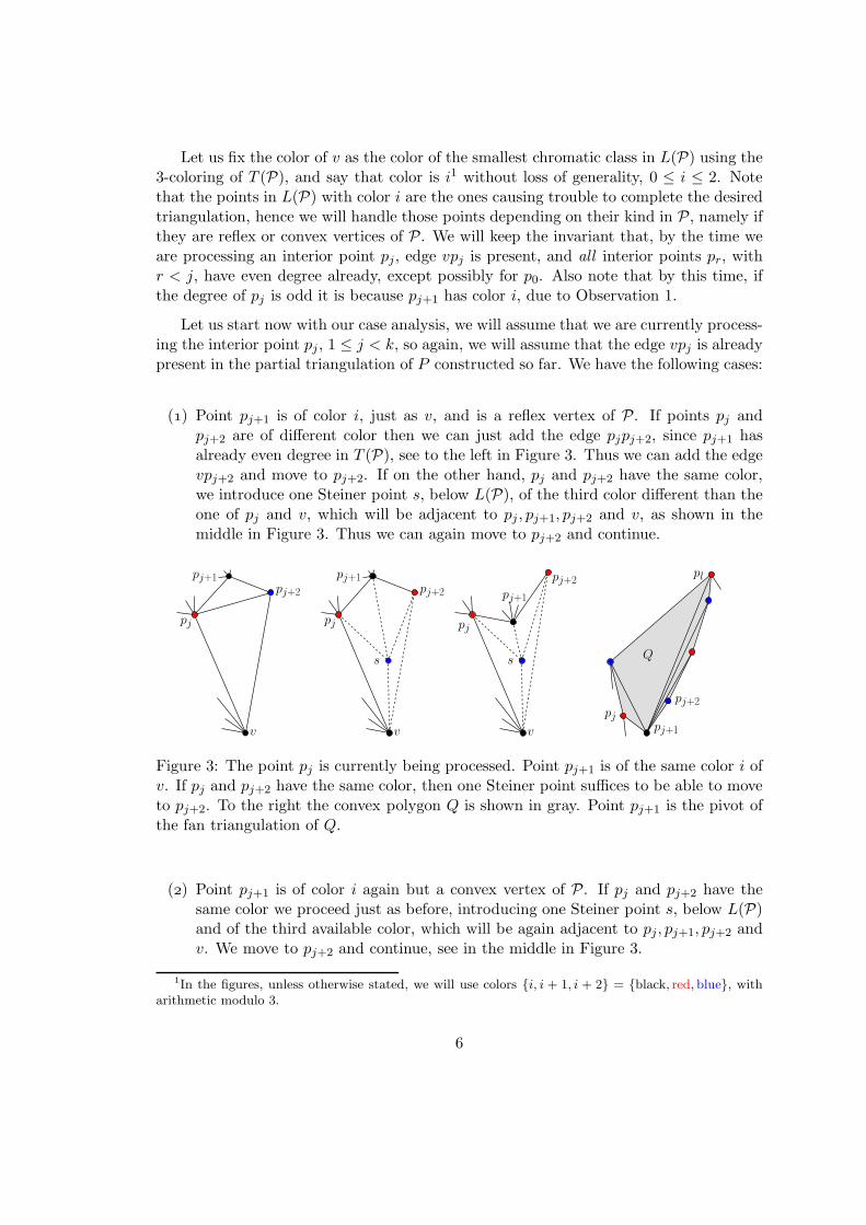
(.) Vertex pj+1 was used as a pivot in the fan triangulation of Q, see to theright in Figure 3. This in particular means that pj+1 is the only vertex ofcolor i in Q. If l > j + 2 then we can re-triangulate Q by constructing thefan triangulation of Q with pivot at pl−1, this changes the 3-coloring of Qonly between pj+1 and pl−1, the former receives color i + 2 while the latteris the new unique vertex of Q of color i. Thus the only thing we did was tomove the vertex of color i to the right, and hence we can join v to all verticespj+1, . . . , pl−2 using straight-line segments. If l = j + 2 then Q is actually atriangle, and everything is still valid, v is connected to pl−2 = pj, see to theleft in Figure 4.

We now further distinguish between the following cases:

(..) Point pl is of color i + 1, pl+1 is of color i and pl+2 is of color i + 2,see in the middle in Figure 4. We introduce two Steiner points s1, s2 ofcolor i+2, i+ 1 respectively and we will make the following adjacencies:() s1 gets adjacent to pl−1, pl, pl+1 and s2, and () s2 gets adjacent topl−2, pl−1, s1, pl+1, pl+2, v. Observe that these adjacencies can always bedone without introducing any crossing. Moreover, note that with twoSteiner points we complete the even degree of each point in the regionpj, . . . , pl+2 in which there were originally two points of color i. Thus wecan move to pl+2 and continue.

(..) Point pl and pl+1 as before, but pl+2 is of color i+1. We will proceed asbefore except that this time the adjacencies of s1, s2 are as follows: ()s1 gets adjacent to s2, pl−1, pl, pl+1, pl+2 and v, and () s2 gets adjacentto pl−2, pl−1, s1 and v.As before, we also introduce the adjacencies pj+1v, . . . , pl−2v and pl+2v.We can again move to pl+2. See to the right in Figure 4 for the finalconfiguration.

(..) Point pl as before but pl+1 is of color i + 2 instead. Note that in thiscase, from pj to pl+1 there is only one vertex of color i, namely pl−1,thus we will introduce only one Steiner point s. Also observe that sincepl is a reflex vertex of P we can add the adjacency pl−1pl+1. Finally wemake s adjacent to pl−2, pl−1, pl+1, v, and we make, as before, v adja-cent to pj+1, . . . , pl−2 and pl+1. See to the left in Figure 5 for the finalconfiguration.The following three cases are complementary:

(..) Point pl is of color i+ 2, pl+1 is of color i and pl+2 is of color i+ 1.

7

pl−1

pj+1

pj

pj+2

pl

Q

pj+1

pj

pj+2

pl

s1

s2

pl+2pl−1

pl+2

pj+1

pj

pj+2

pl

s1

s2

pl−1

Figure 4: If pj+1 was used as a pivot to triangulate a convex polygon that can be cutfrom P, then we can use pl−1 as the new pivot without changing the color of pj oranything to its left. Note that pl must be necessarily a reflex vertex of P. In the middlewe see the final configuration in the case that pl+1 is of color i and pl+2 is of color i+2.To the right we see the final configuration when pl+1 is of color i and pl+2 is of colori+ 1.

pj+1

pj

pj+2

pj+1

pj

pj+2

pl

s

pl−1pl+1

q

s

q = pj−2 pj+1

pj

pj−1

pj+2s1

s2

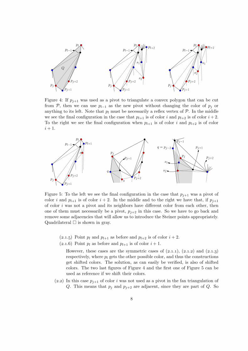
Figure 5: To the left we see the final configuration in the case that pj+1 was a pivot ofcolor i and pl+1 is of color i + 2. In the middle and to the right we have that, if pj+1

of color i was not a pivot and its neighbors have different color from each other, thenone of them must necessarily be a pivot, pj+2 in this case. So we have to go back andremove some adjacencies that will allow us to introduce the Steiner points appropriately.Quadrilateral � is shown in gray.

(..) Point pl and pl+1 as before and pl+2 is of color i+ 2.

(..) Point pl as before and pl+1 is of color i+ 1.

However, these cases are the symmetric cases of (..), (..) and (..)respectively, where pl gets the other possible color, and thus the constructionsget shifted colors. The solution, as can easily be verified, is also of shiftedcolors. The two last figures of Figure 4 and the first one of Figure 5 can beused as reference if we shift their colors.

(.) In this case pj+1 of color i was not used as a pivot in the fan triangulation ofQ. This means that pj and pj+2 are adjacent, since they are part of Q. So

8

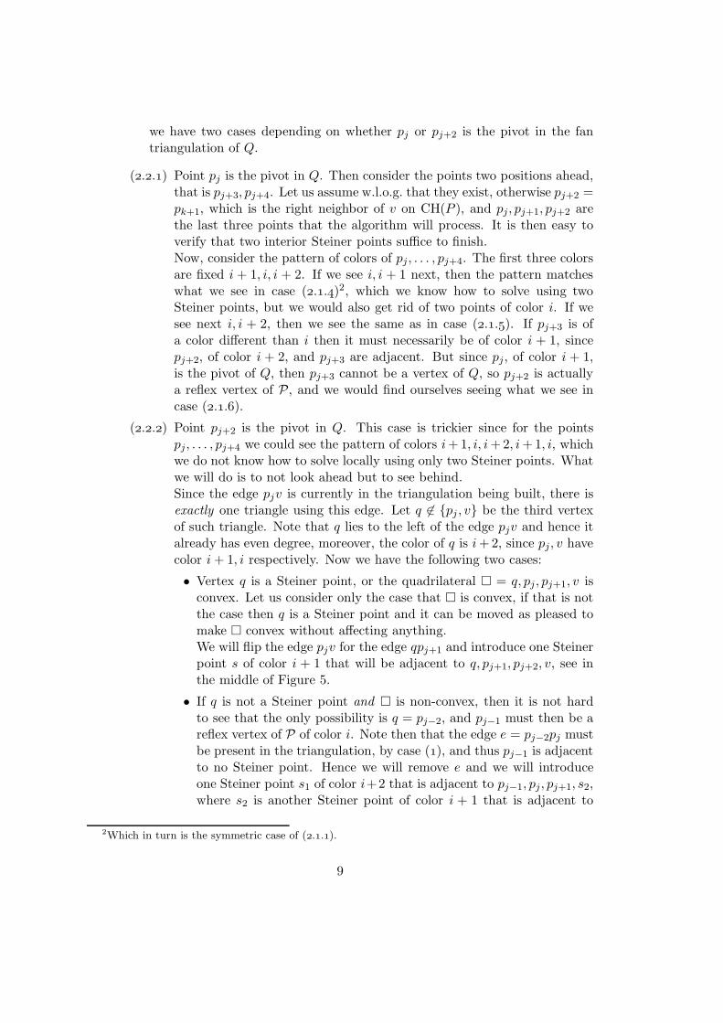
we have two cases depending on whether pj or pj+2 is the pivot in the fantriangulation of Q.

(..) Point pj is the pivot in Q. Then consider the points two positions ahead,that is pj+3, pj+4. Let us assume w.l.o.g. that they exist, otherwise pj+2 =pk+1, which is the right neighbor of v on CH(P ), and pj, pj+1, pj+2 arethe last three points that the algorithm will process. It is then easy toverify that two interior Steiner points suffice to finish.Now, consider the pattern of colors of pj, . . . , pj+4. The first three colorsare fixed i + 1, i, i + 2. If we see i, i + 1 next, then the pattern matcheswhat we see in case (..)2, which we know how to solve using twoSteiner points, but we would also get rid of two points of color i. If wesee next i, i + 2, then we see the same as in case (..). If pj+3 is ofa color different than i then it must necessarily be of color i + 1, sincepj+2, of color i + 2, and pj+3 are adjacent. But since pj, of color i + 1,is the pivot of Q, then pj+3 cannot be a vertex of Q, so pj+2 is actuallya reflex vertex of P, and we would find ourselves seeing what we see incase (..).

(..) Point pj+2 is the pivot in Q. This case is trickier since for the pointspj, . . . , pj+4 we could see the pattern of colors i+1, i, i+2, i+1, i, whichwe do not know how to solve locally using only two Steiner points. Whatwe will do is to not look ahead but to see behind.Since the edge pjv is currently in the triangulation being built, there isexactly one triangle using this edge. Let q 6∈ {pj , v} be the third vertexof such triangle. Note that q lies to the left of the edge pjv and hence italready has even degree, moreover, the color of q is i+2, since pj, v havecolor i+ 1, i respectively. Now we have the following two cases:

• Vertex q is a Steiner point, or the quadrilateral � = q, pj, pj+1, v isconvex. Let us consider only the case that � is convex, if that is notthe case then q is a Steiner point and it can be moved as pleased tomake � convex without affecting anything.We will flip the edge pjv for the edge qpj+1 and introduce one Steinerpoint s of color i + 1 that will be adjacent to q, pj+1, pj+2, v, see inthe middle of Figure 5.

• If q is not a Steiner point and � is non-convex, then it is not hardto see that the only possibility is q = pj−2, and pj−1 must then be areflex vertex of P of color i. Note then that the edge e = pj−2pj mustbe present in the triangulation, by case (), and thus pj−1 is adjacentto no Steiner point. Hence we will remove e and we will introduceone Steiner point s1 of color i+2 that is adjacent to pj−1, pj, pj+1, s2,where s2 is another Steiner point of color i + 1 that is adjacent to

2Which in turn is the symmetric case of (..).

9

pj−2, pj−1, s1, pj+1, pj+2, v. We can now move to pj+2 and continue.See to the right in Figure 5.

Note that the color i of v was chosen as the color of the smallest chromatic class inL(P), so its cardinality can be at most

⌊

k+2

3

⌋

. Now, it is important to observe that weassumed that the point pj that we process is neither p0 nor pk+1 of CH(P ), since thealgorithm started with j ≥ 1. So it could happen that at least one of those extremepoints is of the same color i of v, which would give a conflict in the 3-coloring of thetriangulation we are constructing. Let us see how can we deal with this kind of situation.Assume without loss of generality that p0 is of color i. Then, before start processing thefirst interior points p1, introduce one Steiner point v′ inside CH(P ), so close to v thatthe angular order p1, . . . , pk w.r.t. v is also kept by v′. This Steiner point v′ will replacev in the algorithm, so it will get color i as well. Now symbolically delete v and run thealgorithm. When the algorithm ends we will still have the conflict of the monochromaticedge p0v

′, we could simultaneously have the same conflict with edge v′pk+1.

v′pk+1

v

p1

p0 v′pk+1

v

p1

p0

pk

Figure 6: Polygon P shown in light gray. In the figures color i = black, and the colorwhite means that those points are somehow 3-colored without conflicting with the blackpoints. The visibility region of v is shown in dark gray.

Put back v and remove the conflicting edges from the construction. We will proceeddepending on what v sees, having the edges of the construction as obstacles. That is, ifedge p0v

′ is the only one with conflicts, then v sees the polygonal chain p0, p1, v′, pk+1,

see to the left in Figure 6. If the edge v′pk+1 also has conflicts then v sees the polygonalchain p0, p1, v

′, pk, pk+1, see to the right in Figure 6. The solution will depend on whetherp0v

′ is the only conflict or not, and whether v′ has even degree, in the triangulationconstructed by the algorithm, or not. The four cases, shown in solid lines, and theirsolutions, shown with dashed lines, can be seen in Figure 7. Observe that at most onemore Steiner point s is used for the solutions, and that v′, s are both interior Steinerpoints. So s can be charged to p0, which is one of the

⌊

k+2

3

⌋

points of L(P) of color i,and v′ would be simply one interior Steiner point that cannot be charged to anything.

Finally, in the analysis of cases (..) to (..) we always assumed that point pl+1

always existed. This might not always be the case since we could have pl = pk+1, butin this case we could safely assume that pl+1 = v or pl+1 = v′, depending on conflictson CH(P ), so the second Steiner point we introduce in those cases is also an interior

10

v′pk+1

v

p1

p0

s

v′pk+1

v

p1

p0

s

v′pk+1

v

p1

p0

pk pk

v′pk+1

v

p1

p0

Figure 7: Polygon P shown in gray. On the top part we have the solution for the caseswhere p0v

′ is the only conflict and the degree of v′ is odd, left, or even, right. Belowwe have the solutions for the case when both edges p0v

′, v′pk+1 are in conflict and thedegree of v′ is odd, left, or even, right. In the figures color i = black.

Steiner point that cannot be charged to anything. Hence the construction used at most⌊

k+2

3

⌋

+ 2 interior Steiner points, and Theorem 1 follows.

4.1 Extension to even triangulations

Theorem 1 guarantees a 3-colorable triangulation, which will be at least pseudo-even,but it might not necessarily be completely even, and this is because when we choose anarbitrary triangulation for a part of P, some vertices of CH(P ) might get odd degree.Thus in order to construct an even triangulation we have to do some more work.

As we mentioned before, in an even triangulation the size of the outer face must bemultiple of three. Thus the first thing we will do, if necessary, is to complete CH(P )using at most two Steiner points so that we fulfill |CH(P )| ≡ 0 mod 3.

Let v again the unique vertex of CH(P ) with the smallest y-coordinate, and sort allP \ {v} angularly, from left to right, around v. Let p1, . . . , pn−1 be the points of P \ {v}in this sorted order.

The main idea behind the construction is to enclose P in a bigger polygon Q so thatall p0, . . . , pn−1 are interior points, and then run the algorithm of Theorem 1, which willguarantee that all p0, . . . , pn−1 will have even degree. The construction is done in sucha way that CH(P ) appears in the construction, at the end we can complete the degreeof v to an even degree, if necessary, and such that by removing Q we do not destroy

11

any parity, since Q, upon deletion, will take with it an even number of adjacencies per“affected” point of CH(P ), so the degree of those affected points will remain even at theend. So let us jump to the actual construction.

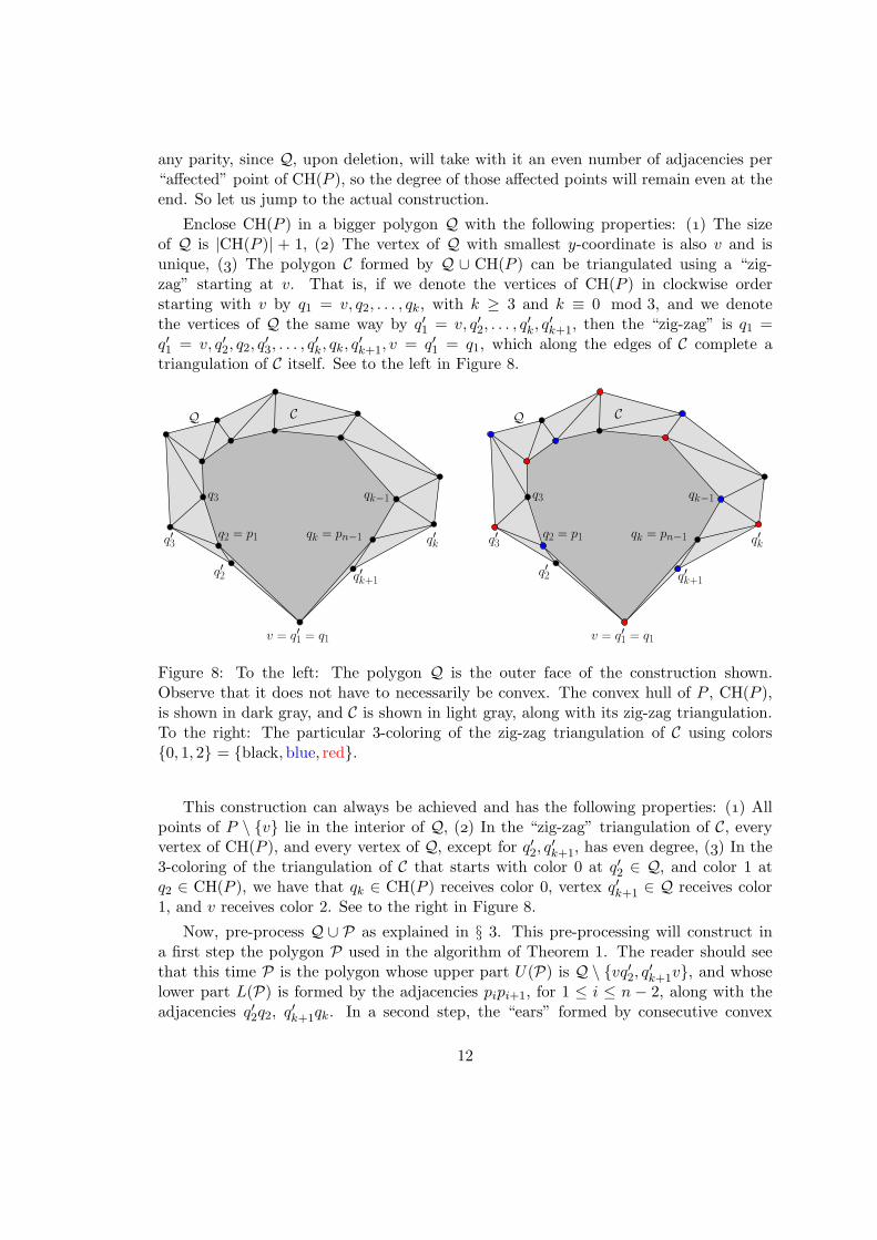
Enclose CH(P ) in a bigger polygon Q with the following properties: () The sizeof Q is |CH(P )| + 1, () The vertex of Q with smallest y-coordinate is also v and isunique, () The polygon C formed by Q ∪ CH(P ) can be triangulated using a “zig-zag” starting at v. That is, if we denote the vertices of CH(P ) in clockwise orderstarting with v by q1 = v, q2, . . . , qk, with k ≥ 3 and k ≡ 0 mod 3, and we denotethe vertices of Q the same way by q′1 = v, q′2, . . . , q

′

k, q′

k+1, then the “zig-zag” is q1 =

q′1 = v, q′2, q2, q′

3, . . . , q′

k, qk, q′

k+1, v = q′1 = q1, which along the edges of C complete a

triangulation of C itself. See to the left in Figure 8.

q′3

q′k+1

q′kqk = pn−1

q3 qk−1

v = q′1 = q1

q2 = p1

q′2

Q C

q′3

q′k+1

q′kqk = pn−1

q3 qk−1

v = q′1 = q1

q2 = p1

q′2

Q C

Figure 8: To the left: The polygon Q is the outer face of the construction shown.Observe that it does not have to necessarily be convex. The convex hull of P , CH(P ),is shown in dark gray, and C is shown in light gray, along with its zig-zag triangulation.To the right: The particular 3-coloring of the zig-zag triangulation of C using colors{0, 1, 2} = {black,blue, red}.

This construction can always be achieved and has the following properties: () Allpoints of P \ {v} lie in the interior of Q, () In the “zig-zag” triangulation of C, everyvertex of CH(P ), and every vertex of Q, except for q′2, q

′

k+1, has even degree, () In the

3-coloring of the triangulation of C that starts with color 0 at q′2 ∈ Q, and color 1 atq2 ∈ CH(P ), we have that qk ∈ CH(P ) receives color 0, vertex q′k+1

∈ Q receives color1, and v receives color 2. See to the right in Figure 8.

Now, pre-process Q ∪ P as explained in § 3. This pre-processing will construct ina first step the polygon P used in the algorithm of Theorem 1. The reader should seethat this time P is the polygon whose upper part U(P) is Q \ {vq′2, q

′

k+1v}, and whose

lower part L(P) is formed by the adjacencies pipi+1, for 1 ≤ i ≤ n − 2, along with theadjacencies q′2q2, q

′

k+1qk. In a second step, the “ears” formed by consecutive convex

12

vertices of L(P) will be computed. Recall that this “ears” are the convex polygons Qj ’sin the pre-processing phase. Here, by suitably locating q′2, q

′

k+1∈ Q we can assume that

both q2, qk ∈ CH(P ) are reflex vertices of P, see Figure 9. Moreover, observe that any

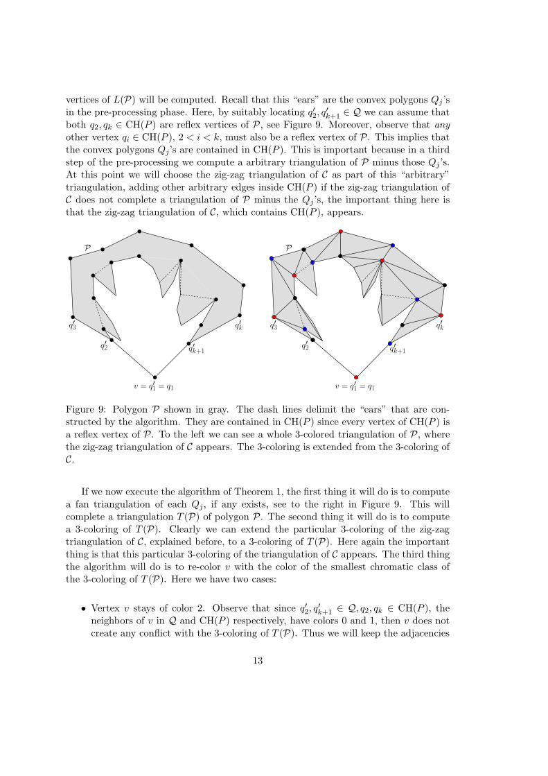
other vertex qi ∈ CH(P ), 2 < i < k, must also be a reflex vertex of P. This implies thatthe convex polygons Qj’s are contained in CH(P ). This is important because in a thirdstep of the pre-processing we compute a arbitrary triangulation of P minus those Qj’s.At this point we will choose the zig-zag triangulation of C as part of this “arbitrary”triangulation, adding other arbitrary edges inside CH(P ) if the zig-zag triangulation ofC does not complete a triangulation of P minus the Qj ’s, the important thing here isthat the zig-zag triangulation of C, which contains CH(P ), appears.

q′3

q′k+1

q′k

v = q′1 = q1

q′2

P

q′3

q′k+1

q′k

v = q′1 = q1

q′2

P

Figure 9: Polygon P shown in gray. The dash lines delimit the “ears” that are con-structed by the algorithm. They are contained in CH(P ) since every vertex of CH(P ) isa reflex vertex of P. To the left we can see a whole 3-colored triangulation of P, wherethe zig-zag triangulation of C appears. The 3-coloring is extended from the 3-coloring ofC.

If we now execute the algorithm of Theorem 1, the first thing it will do is to computea fan triangulation of each Qj, if any exists, see to the right in Figure 9. This willcomplete a triangulation T (P) of polygon P. The second thing it will do is to computea 3-coloring of T (P). Clearly we can extend the particular 3-coloring of the zig-zagtriangulation of C, explained before, to a 3-coloring of T (P). Here again the importantthing is that this particular 3-coloring of the triangulation of C appears. The third thingthe algorithm will do is to re-color v with the color of the smallest chromatic class ofthe 3-coloring of T (P). Here we have two cases:

• Vertex v stays of color 2. Observe that since q′2, q′

k+1∈ Q, q2, qk ∈ CH(P ), the

neighbors of v in Q and CH(P ) respectively, have colors 0 and 1, then v does notcreate any conflict with the 3-coloring of T (P). Thus we will keep the adjacencies

13

q′2v, q2v, vqk and vq′k+1, and we will execute the algorithm to the end. Since the

colors of q′2, q′

k+1, q2, qk, v are never changed by the algorithm, we end up having a

3-colored triangulation, where v also has even degree, that uses at most⌊

n+1

3

⌋

+13

interior Steiner points. Note that these interior Steiner points are also interiorw.r.t. CH(P ), since the algorithm of Theorem 1 would introduce the Steiner pointsinside Q, but strictly below the lower part L(P) of P. Since the adjacenciesq′2v, q2v, vqk and vq′k+1

are present in the output triangulation, the Steiner pointsfall strictly inside CH(P ).

The reader can verify that if we now remove Q\{v}, along with all the adjacenciesthat it takes with it, we are left with the desired even triangulation.

• Vertex v changes color. Then we will assume without loss of generality that v

gets color 0. If v got color 1 we would have a symmetric conversation. Rememberthat by the particular 3-coloring of C we have that q′2, q

′

k+1∈ Q have colors 0, 1

respectively, and q2, qk ∈ CH(P ) have color 1, 0 respectively, see Figure 8. Thusthe algorithm will introduce the Steiner point v′ of color 0, to take the place of v,and will symbolically delete v. This time we can charge v′ to q′2 which is one of the⌊

n+1

3

⌋

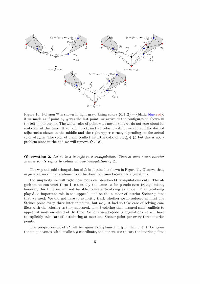
points of L(P) of color 0. Now introduce the adjacency v′pn−2 and executethe algorithm until it finishes. There, point pn−2 would be the last processed point.So we arrive at the configuration shown in the left upper corner of Figure 10.

In this configuration we necessarily have that the degree of q2 = p1 ∈ CH(P ) isodd, since it is adjacent to q′2, v

′ ∈ Q which have both color 0. The degree of pn−2

is also odd since it is adjacent to v′, qk = pn−1 ∈ CH(P ), and both are colored 0as well. So the only options we have now are whether v′ has even or odd degreebetween q2 and pn−2. This is equivalent to consider whether pn−2 is of color 2 or1 respectively. Those two configurations are shown in the right upper corner, andin the middle respectively, in Figure 10 in solid.

Now let us put v back and we will finish the construction as shown in Figure 10with dashed lines. We might require the use of another Steiner point s, as shown tothe right in the upper corner of the same figure, which can be charged to qk = pn−1.In the end v gets even degree as well. It is not hard to verify that the total numberof interior Steiner points is again at most

⌊

n+1

3

⌋

+ 1, that all Steiner points areinterior to CH(P ), and that the removal of Q \ {v} does not destroy any parity.Hence Theorem 2 follows.

5 Pseudo-odd and odd triangulations

Working locally with (pseudo-)odd triangulations is slightly easier. The following obser-vation was already pointed out in [7]:

3It is not⌊

n+1

3

⌋

+ 2 this time since there is no conflict in CH(P ).

14

v′

q′3

q′k+1

q′k

qk = pn−1q3 qk−1

pn−2

v′

q′3

q′k+1

q′k

qk = pn−1q3 qk−1

pn−2

v′

q′2q′3

q′k+1

q′k

qk = pn−1

q2 = p1

q3 qk−1

pn−2

s

v = q′1 = q1

q2 = p1

q′2q2 = p1

q′2

v = q′1 = q1

v = q′1 = q1

Figure 10: Polygon P is shown in light gray. Using colors {0, 1, 2} = {black,blue, red},if we made as if point pn−2 was the last point, we arrive at the configuration shown inthe left upper corner. The white color of point pn−2 means that we do not care about itsreal color at this time. If we put v back, and we color it with 3, we can add the dashedadjacencies shown in the middle and the right upper corner, depending on the actualcolor of pn−2. The color of v will conflict with the color of q′3, q

′

k ∈ Q, but this is not aproblem since in the end we will remove Q \ {v}.

Observation 2. Let △ be a triangle in a triangulation. Then at most seven interior

Steiner points suffice to obtain an odd-triangulation of △.

The way this odd triangulation of △ is obtained is shown in Figure 11. Observe that,in general, no similar statement can be done for (pseudo-)even triangulations.

For simplicity we will right now focus on pseudo-odd triangulations only. The al-gorithm to construct them is essentially the same as for pseudo-even triangulations,however, this time we will not be able to use a 3-coloring as guide. That 3-coloringplayed an important role in the upper bound on the number of interior Steiner pointsthat we used: We did not have to explicitly track whether we introduced at most oneSteiner point every three interior points, but we just had to take care of solving con-flicts with the coloring as they appeared. The 3-coloring then ensured such conflicts toappear at most one-third of the time. So for (pseudo-)odd triangulations we will haveto explicitly take care of introducing at most one Steiner point per every three interiorpoints.

The pre-processing of P will be again as explained in § 3. Let v ∈ P be againthe unique vertex with smallest y-coordinate, the one we use to sort the interior points

15

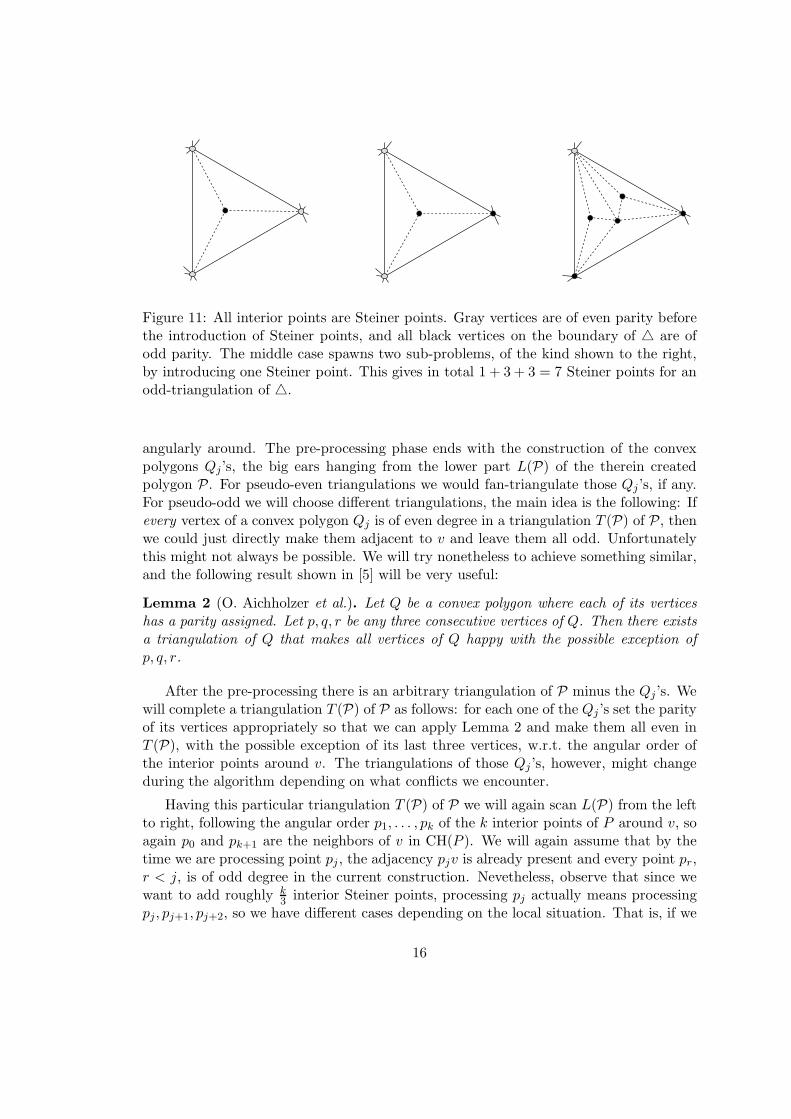
Figure 11: All interior points are Steiner points. Gray vertices are of even parity beforethe introduction of Steiner points, and all black vertices on the boundary of △ are ofodd parity. The middle case spawns two sub-problems, of the kind shown to the right,by introducing one Steiner point. This gives in total 1 + 3 + 3 = 7 Steiner points for anodd-triangulation of △.

angularly around. The pre-processing phase ends with the construction of the convexpolygons Qj’s, the big ears hanging from the lower part L(P) of the therein createdpolygon P. For pseudo-even triangulations we would fan-triangulate those Qj ’s, if any.For pseudo-odd we will choose different triangulations, the main idea is the following: Ifevery vertex of a convex polygon Qj is of even degree in a triangulation T (P) of P, thenwe could just directly make them adjacent to v and leave them all odd. Unfortunatelythis might not always be possible. We will try nonetheless to achieve something similar,and the following result shown in [5] will be very useful:

Lemma 2 (O. Aichholzer et al.). Let Q be a convex polygon where each of its vertices

has a parity assigned. Let p, q, r be any three consecutive vertices of Q. Then there exists

a triangulation of Q that makes all vertices of Q happy with the possible exception of

p, q, r.

After the pre-processing there is an arbitrary triangulation of P minus the Qj’s. Wewill complete a triangulation T (P) of P as follows: for each one of the Qj ’s set the parityof its vertices appropriately so that we can apply Lemma 2 and make them all even inT (P), with the possible exception of its last three vertices, w.r.t. the angular order ofthe interior points around v. The triangulations of those Qj ’s, however, might changeduring the algorithm depending on what conflicts we encounter.

Having this particular triangulation T (P) of P we will again scan L(P) from the leftto right, following the angular order p1, . . . , pk of the k interior points of P around v, soagain p0 and pk+1 are the neighbors of v in CH(P ). We will again assume that by thetime we are processing point pj , the adjacency pjv is already present and every point pr,r < j, is of odd degree in the current construction. Nevetheless, observe that since wewant to add roughly k

3interior Steiner points, processing pj actually means processing

pj, pj+1, pj+2, so we have different cases depending on the local situation. That is, if we

16

are currently stuck at pj it is because its current degree is even, otherwise we could justcontinue. So the cases we have to study are the triples of parities: (e, e, e), (e, e, o), (e, o, e)and (e, o, o), where they correspond entry-wise to the current parities of (pj, pj+1, pj+2),and e, o stand for even and odd respectively. It is very important to keep in mind thatin the triple (pj , pj+1, pj+2), the only point adjacent to v is pj. Also, in all cases we willassume that pj+3 exists. If that is not the case then one of pj, pj+1, pj+2 is pk+1, and wewould find ourselves with a problem of constant size that can be solved using a constantnumber of interior Steiner points, due to Observation 2. We will now jump to the casedistinction.

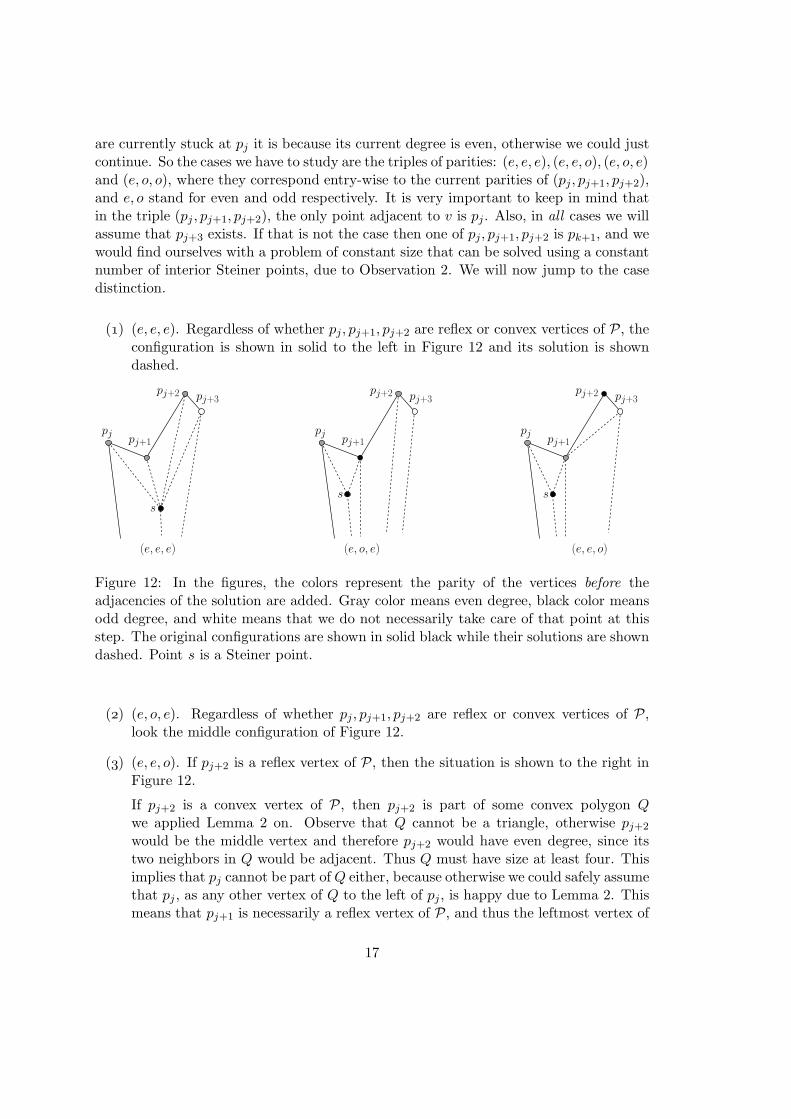
() (e, e, e). Regardless of whether pj, pj+1, pj+2 are reflex or convex vertices of P, theconfiguration is shown in solid to the left in Figure 12 and its solution is showndashed.

pj+1

pj+2

pj

pj+3

(e, e, e) (e, o, e) (e, e, o)

s

pj+1

pj+2

pj

pj+3

s

pj+1

pj+2

pj

pj+3

s

Figure 12: In the figures, the colors represent the parity of the vertices before theadjacencies of the solution are added. Gray color means even degree, black color meansodd degree, and white means that we do not necessarily take care of that point at thisstep. The original configurations are shown in solid black while their solutions are showndashed. Point s is a Steiner point.

() (e, o, e). Regardless of whether pj, pj+1, pj+2 are reflex or convex vertices of P,look the middle configuration of Figure 12.

() (e, e, o). If pj+2 is a reflex vertex of P, then the situation is shown to the right inFigure 12.

If pj+2 is a convex vertex of P, then pj+2 is part of some convex polygon Q

we applied Lemma 2 on. Observe that Q cannot be a triangle, otherwise pj+2

would be the middle vertex and therefore pj+2 would have even degree, since itstwo neighbors in Q would be adjacent. Thus Q must have size at least four. Thisimplies that pj cannot be part ofQ either, because otherwise we could safely assumethat pj , as any other vertex of Q to the left of pj, is happy due to Lemma 2. Thismeans that pj+1 is necessarily a reflex vertex of P, and thus the leftmost vertex of

17

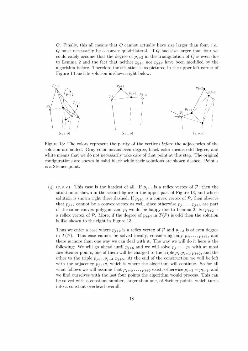
Q. Finally, this all means that Q cannot actually have size larger than four, i.e.,Q must necessarily be a convex quadrilateral. If Q had size larger than four wecould safely assume that the degree of pj+2 in the triangulation of Q is even dueto Lemma 2 and the fact that neither pj+1 nor pj+2 have been modified by thealgorithm before. Therefore the situation is as pictured in the upper left corner ofFigure 13 and its solution is shown right below.

(e, e, o) (e, o, o) (e, o, o)

pj+1

pj+2

pj

pj+3

pj+1

pj+2pj

pj+3

s

pjpj+1

pj+2pj+3

Figure 13: The colors represent the parity of the vertices before the adjacencies of thesolution are added. Gray color means even degree, black color means odd degree, andwhite means that we do not necessarily take care of that point at this step. The originalconfigurations are shown in solid black while their solutions are shown dashed. Point sis a Steiner point.

() (e, o, o). This case is the hardest of all. If pj+1 is a reflex vertex of P, then thesituation is shown in the second figure in the upper part of Figure 13, and whosesolution is shown right there dashed. If pj+1 is a convex vertex of P, then observethat pj+2 cannot be a convex vertex as well, since otherwise pj, . . . , pj+3 are partof the same convex polygon, and pj would be happy due to Lemma 2. So pj+2 isa reflex vertex of P. More, if the degree of pj+3 in T (P) is odd then the solutionis like shown to the right in Figure 13.

Thus we enter a case where pj+2 is a reflex vertex of P and pj+3 is of even degreein T (P). This case cannot be solved locally, considering only pj , . . . , pj+3, andthere is more than one way we can deal with it. The way we will do it here is thefollowing: We will go ahead until pj+6 and we will solve pj, . . . , p6 with at mosttwo Steiner points, one of them will be charged to the triple pj, pj+1, pj+2, and theother to the triple pj+3, pj+4, pj+5. At the end of the construction we will be leftwith the adjacency pj+6v, which is where the algorithm will continue. So for allwhat follows we will assume that pj+4, . . . , pj+6 exist, otherwise pj+3 = pk+1, andwe find ourselves with the last four points the algorithm would process. This canbe solved with a constant number, larger than one, of Steiner points, which turnsinto a constant overhead overall.

18

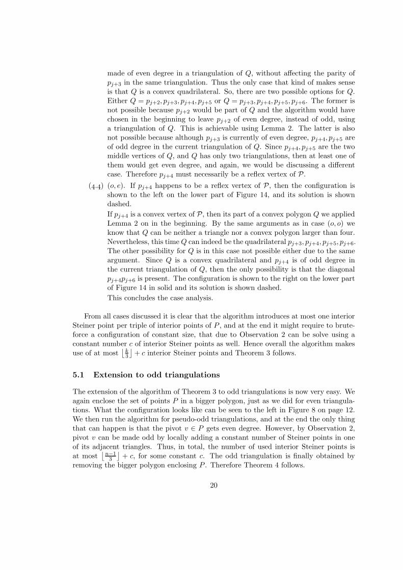
Since we are assuming that pj+3 is currently even, we have four main sub-casesthat depend on the pair of parities (·, ·) of (pj+4, pj+5) in T (P). The configurationsand solutions are pictured in Figure 14.

(e, o, o, e) + (e, e)

pj

pj+1

pj+2

pj+3

pj+6

s1

s2

pj

pj+1

pj+2

pj+3

s1 s2

pj

pj+1

pj+2

pj+3

pj+6

s1

s2

(e, o, o, e) + (e, o) (e, o, o, e) + (o, o)

pj+4

pj

pj+1

pj+2

pj+3

s

(e, o, o, e) + (o, e)

pj+4

pj

pj+1

pj+2

pj+3

s1

(e, o, o, e) + (o, e)

pj+4

s2

Figure 14: The colors represent the parity of the vertices before the adjacencies of thesolution are added. Gray color means even degree, black color means odd degree, andwhite means that we do not necessarily take care of that point at this step. The originalconfigurations are shown in solid black while their solutions are shown dashed. Pointss1, s2 are Steiner points.

(.) (e, e). The configuration is shown in the left upper corner of Figure 14 insolid and its solution is shown dashed. Observe that for the solution it doesnot play a role whether pj+3, pj+4, pj+5 are reflex or convex vertices of P.

(.) (e, o). The configuration is shown in the second figure on the upper part ofFigure 14 in solid and its solution is shown dashed. Again, it does not matterwhether pj+3, pj+4, pj+5 are reflex or convex vertices of P.

(.) (o, o). If pj+4 is a reflex vertex of P, the configuration is shown in solid tothe right on the upper part of Figure 14, and its solution is shown dashed.

Now let us argue that pj+4 cannot be a convex vertex. If pj+4 were a convexvertex it would be part of a convex polygon Q we applied Lemma 2 on in thebeginning. This polygon Q cannot be a triangle, because then pj+4 wouldbe the middle point and it would then have even degree in T (P). Also, Qcannot have at least five sides because by Lemma 2, again, pj+4 could be

19

made of even degree in a triangulation of Q, without affecting the parity ofpj+3 in the same triangulation. Thus the only case that kind of makes senseis that Q is a convex quadrilateral. So, there are two possible options for Q.Either Q = pj+2, pj+3, pj+4, pj+5 or Q = pj+3, pj+4, pj+5, pj+6. The former isnot possible because pj+2 would be part of Q and the algorithm would havechosen in the beginning to leave pj+2 of even degree, instead of odd, usinga triangulation of Q. This is achievable using Lemma 2. The latter is alsonot possible because although pj+3 is currently of even degree, pj+4, pj+5 areof odd degree in the current triangulation of Q. Since pj+4, pj+5 are the twomiddle vertices of Q, and Q has only two triangulations, then at least one ofthem would get even degree, and again, we would be discussing a differentcase. Therefore pj+4 must necessarily be a reflex vertex of P.

(.) (o, e). If pj+4 happens to be a reflex vertex of P, then the configuration isshown to the left on the lower part of Figure 14, and its solution is showndashed.

If pj+4 is a convex vertex of P, then its part of a convex polygon Q we appliedLemma 2 on in the beginning. By the same arguments as in case (o, o) weknow that Q can be neither a triangle nor a convex polygon larger than four.Nevertheless, this timeQ can indeed be the quadrilateral pj+3, pj+4, pj+5, pj+6.The other possibility for Q is in this case not possible either due to the sameargument. Since Q is a convex quadrilateral and pj+4 is of odd degree inthe current triangulation of Q, then the only possibility is that the diagonalpj+4pj+6 is present. The configuration is shown to the right on the lower partof Figure 14 in solid and its solution is shown dashed.

This concludes the case analysis.

From all cases discussed it is clear that the algorithm introduces at most one interiorSteiner point per triple of interior points of P , and at the end it might require to brute-force a configuration of constant size, that due to Observation 2 can be solve using aconstant number c of interior Steiner points as well. Hence overall the algorithm makesuse of at most

⌊

k3

⌋

+ c interior Steiner points and Theorem 3 follows.

5.1 Extension to odd triangulations

The extension of the algorithm of Theorem 3 to odd triangulations is now very easy. Weagain enclose the set of points P in a bigger polygon, just as we did for even triangula-tions. What the configuration looks like can be seen to the left in Figure 8 on page 12.We then run the algorithm for pseudo-odd triangulations, and at the end the only thingthat can happen is that the pivot v ∈ P gets even degree. However, by Observation 2,pivot v can be made odd by locally adding a constant number of Steiner points in oneof its adjacent triangles. Thus, in total, the number of used interior Steiner points isat most

⌊

n−1

3

⌋

+ c, for some constant c. The odd triangulation is finally obtained byremoving the bigger polygon enclosing P . Therefore Theorem 4 follows.

20

6 Conclusions

In this paper we have presented algorithms that construct, with help of Steiner points,(pseudo-)even and (pseudo-)odd triangulations of a given set of points P . The numberof Steiner points that the algorithms use is roughly k

3for the pseudo variants, where k

is the number of interior points of P , and roughly n3for the other cases. It is important

to observe that our algorithms do not modify the convex hull of P , and therefore theypreserve extent measures of P , such as diameter, width, among others. If we do notcare about modifying CH(P ), or about the position of the Steiner points, then the taskis in general significantly easier. For example, only two Steiner points far away fromCH(P ) would suffice to construct a pseudo-even triangulation, say one at ∞ and theother at −∞. Albeit being this construction possible, we do not know why it would beinteresting to use it, since the output set of points does not look anything like the onethat was given as the input.

We could believe that the techniques shown here could be pushed further to improvethe overall number of Steiner points, say to go from one-third to one-sixth, but this willimply a significantly larger number of cases to analyze, we see this really as a secondaryinteresting improvement. What we really see as the primary open problems are thefollowing:

• Is it possible to always construct (pseudo-)even or (pseudo-)odd triangulations ofa given set of points P using only a constant number of (interior) Steiner points?In other words, how big is the lower bound on the number of (interior) Steinerpoints that are required to always construct such triangulations? We have failedso far trying to prove a (sub-)linear lower bound, which is the natural guess whenworking on these kind of problems.

• Moving away from using Steiner points, would it be possible to construct even orodd triangulations of a given set of points P where at most a constant numberof points remain unhappy? This question was posed by Aichholzer et al. in [5].In that same paper they proved a lower bound of roughly n

108unhappy vertices

when the assignment of parities is not uniform. Thus, as they pointed out, theinteresting cases are all even and all odd.

Note that although these two question look similar, they might not be equivalent. Ifwe are interested in an even triangulation of P and we construct one where a constantnumber of vertices remain unhappy, those unhappy vertices might be far from each other.This means that we might have to bring them together, at least in pairs, using Steinerpoints. We have to get rid of them of them in pairs, at least, since the number of oddvertices is always even. But to get them close to each other we might require morethan a constant number of Steiner points. Thus the techniques to solve those two openproblems might be rather different. We see a real challenge there.

21

7 Acknowledgement

The author would like to thank Jorge Urrutia and Marco Heredia for suggesting theproblem and for helpful comments in the initial stage of this work, and to RaimundSeidel for valuable feedback.

This research was partially supported by CONACYT-DAAD of Mexico.

References

[1] P. J. Heawood, “On the four-color map theorem,” Quart. J. Pure Math., vol. 29,pp. 270–285, 1898. 1, 2

[2] R. Steinberg, “The state of the three color problem,” in Quo Vadis, Graph Theory?

A Source Book for Challenges and Directions (J. W. K. John Gimbel and L. V.Quintas, eds.), vol. 55 of Annals of Discrete Mathematics, pp. 211 – 248, Elsevier,1993. 1, 2

[3] K. Diks, L. Kowalik, and M. Kurowski, “A new 3-color criterion for planar graphs,”inWG (L. Kucera, ed.), vol. 2573 of Lecture Notes in Computer Science, pp. 138–149,Springer, 2002. 1, 2, 3

[4] O. Aichholzer, T. Hackl, C. Huemer, F. Hurtado, and B. Vogtenhuber, “Large bichro-matic point sets admit empty monochromatic 4-gons,” SIAM J. Discrete Math.,vol. 23, no. 4, pp. 2147–2155, 2010. 1, 2

[5] O. Aichholzer, T. Hackl, M. Hoffmann, A. Pilz, G. Rote, B. Speckmann, andB. Vogtenhuber, “Plane graphs with parity constraints,” in WADS (F. K. H. A.Dehne, M. L. Gavrilova, J.-R. Sack, and C. D. Toth, eds.), vol. 5664 of Lecture

Notes in Computer Science, pp. 13–24, Springer, 2009. 1, 2, 16, 21

[6] S. Fisk, “A short proof of chvatal’s watchman theorem,” J. Comb. Theory, Ser. B,vol. 24, no. 3, p. 374, 1978. 5

[7] A. Pilz, “Parity properties of geometric graphs,” Master’s thesis, Graz University ofTechnology, 2009. 14

22