Parental Education and the Rising Transmission of Income ...

Parental Education and the Rising Transmission of Income

between Generations

Marie Connolly, Catherine Haeck, and Jean-William Laliberte∗

February 2021

Abstract

Intergenerational mobility has decreased over time for the cohorts of children born betweenthe 1960s and the 1980s in Canada. At the same time, returns to education have gone up.Both factors have contributed to exacerbating income gaps between children of parents withand without secondary education. However, the transmission of residual parental income dif-ferences that cannot be accounted for by differences in educational attainment have increasedat a faster rate than overall intergenerational income transmission. In addition, overall incomemobility has shrunk less in communities that have experienced greater increases in parentalhigh school completion rates over time. There is no significant relationship with changes inuniversity education. Overall, these patterns suggest that fostering high school completionmay help slow down the worsening of intergenerational income mobility.JEL codes: J62, D63, I24, I26Keywords: social mobility, intergenerational income transmission, income inequality, educa-tion, Canada

∗Connolly: Universite du Quebec a Montreal. Haeck: Universite du Quebec a Montreal. Laliberte: Universityof Calgary. The authors would like to thank Phil Oreopoulos, Frederic Brousseau, the Social Sciences and Human-ities Research Council for their funding (grant 430-2018-01052), and the Social Analysis and Modelling Divisionat Statistics Canada, in particular Yuri Ostrovsky, Winnie Chan, and Grant Schellenberg, for making this workpossible. They would also like to thank the Fonds de Recherche du Quebec (grant 280848). All errors remain ourown. The analysis presented in this paper was in part conducted at the Quebec Interuniversity Centre for SocialStatistics which is part of the Canadian Research Data Centre Network (CRDCN). The services and activitiesprovided by the QICSS are made possible by the financial or in-kind support of the Social Sciences and Humani-ties Research Council (SSHRC), the Canadian Institutes of Health Research (CIHR), the Canada Foundation forInnovation (CFI), Statistics Canada, the Fonds de recherche du Quebec - Societe et culture (FRQSC), the Fondsde recherche du Quebec - Sante (FRQS) and the Quebec universities. The views expressed in this paper are thoseof the authors, and not necessarily those of the CRDCN or its partners.

1 Introduction

Understanding and ensuring equality of opportunity is a priority for many public policy decision

makers and citizens alike. The potential mechanisms through which income is transmitted across

generations are many. Identifying which of these factors matter most for equality of opportunity

is key to designing public policies aimed at fostering intergenerational mobility.

Chetty et al. (2014), Connolly et al. (2019a), and Corak (2020) show that intergenerational

income mobility varies greatly across locations within the United States and Canada. These spatial

differences in mobility tend to correlate strongly with segregation, income inequality, school quality,

social capital, family stability, and educational attainment. Other work suggests that income

mobility also varies over time, in the United States (Chetty et al. 2017; Davis and Mazumder

2019; Olivetti and Paserman 2015) as well as in Canada (Connolly et al. 2019b; Ostrovsky 2017)

and in other countries (see Guell et al. 2015; Pekkarinen et al. 2017, among others).

In this chapter, we start by documenting the evolution of intergenerational mobility in Canada

using tax data that cover the universe of children born during a period spanning over 20 years,

allowing us to track changes in income mobility over two decades with a high degree of precision.

We show that the transmission of income across generations has strengthened over time, with the

correlation of income ranks between parents and children increasing by just under 20%.1

Second, we examine the interplay between educational attainment of parents, more specifically

of mothers, and income rank mobility. To do so, we develop a novel data linkage between Canadian

tax data and Census data. Using this combined data set, we are able to provide the first-ever

detailed picture of the evolution of mobility across Canada by parental education level. Here, we

show that the economic returns to maternal education have gone up–for the mothers themselves

as well as for their children. In tandem with decreasing income mobility, this phenomenon has

contributed to exacerbating income gaps in adulthood between children of parents with and without

secondary education. On average, children of educated mothers attain higher incomes than children

of less educated mothers at every point in the parental income distribution. In other words, parental

education boosts children income ranks above and beyond what would be expected on the basis

of parental income alone. This relative advantage is stronger for children whose parents are in the

bottom half of the income distribution.

Third, we implement two accounting analyses to quantify the role played by changes in maternal

education for the evolution of income mobility in Canada. Mobility was greater for cohorts of

children born in the early 1960s than for those born in the 1980s, and this reduction in mobility

was particularly pronounced for families in which the mother did not hold a high school diploma.

A naive simulation exercise indicates that increases in average parental education over the study

1See also Connolly et al. (2019b) for a detailed account of changes in mobility over the same time period.

1

period have attenuated the observed reduction in relative mobility, which suggests that aggregate

education may fuel relative intergenerational income mobility. In addition, we show that the rank-

rank relationship between child and parent income conditional on maternal education has increased

at a faster rate than the unconditional relationship did. This pattern suggests that, if anything,

observed changes in maternal education have helped slow down the reduction in intergenerational

income mobility in Canada.

Fourth, we turn to province-level estimates of mobility to further examine the relationship

between maternal education and mobility. Here, we use variation over time and space to estimate

the relationship between province-level aggregate maternal education and relative income mobility.

Changes in overall levels of education can affect mobility in several ways. For instance, increasing

the supply of educated parents can reduce the returns to education in the parent generation,

thereby partly closing the gap in parental financial resources between children of low- and high-

education parents. It can also reduce the relative value of the human capital benefits that children

of educated parents enjoy above and beyond the extra financial resources. Finally, aggregate

maternal education could directly modulate the importance of parental financial resources for

children outcomes, conditional on individual parental education.

Our results show that income mobility has shrunk less in communities that have experi-

enced greater increases in maternal high school completion rates over time. We find that a

one-percentage-point increase in the fraction of mothers with a high school diploma reduces the

parent-child rank-rank slope (the intergenerational income correlation) by 2.3%, thus increasing

socioeconomic mobility. There is less evidence of a significant relationship between the fraction of

mothers holding a bachelor degree and mobility. A decomposition analysis suggests that maternal

education mostly affects mobility by shaping the strength of the conditional parent-child income

link within education groups, rather than by decreasing the relative value of the benefits children

of educated parents individually enjoy.

Our work builds upon a long line of research on intergenerational mobility in economics that

traces its roots back to Becker and Tomes (1979, 1986) and Loury (1981); sociologists go even fur-

ther back, with Blau and Duncan (1967), Featherman et al. (1975), Goldthorpe (1980), Goldthorpe

and Hope (1974), and Sewell and Hauser (1975), contributions that focus on the intergenerational

transmission of social status as proxied by occupational prestige. Parental education is also com-

monly used as a measure of social origins, by economists and sociologists alike (Blanden 2013;

Bradbury et al. 2015; Bukodi and Goldthorpe 2013; Goldthorpe 2013).

The development of large longitudinal administrative data, particularly intergenerationally-

linked tax data, has placed the focus of recent literature on the intergenerational transmission of

income, especially the correlation between parental income rank and child income rank (Chetty et

al. 2014). Chetty et al. (2014) show that there are important differences within the United States

2

in terms of rank mobility and the opportunities available to children from different socioeconomic

backgrounds. Corak (2020) does the same for Canada, while Connolly et al. (2019a) highlight

the fact that high-mobility and low-mobility areas exist in both countries, but that the population

residing in low-mobility areas is much larger in the U.S., leading to much lower nationwide mobility

rates. Another important finding is that mobility rates appear to be on decline when comparing

successive birth cohorts, both in Canada (Connolly et al. 2019b) and in the U.S. (Chetty et

al. 2017; Davis and Mazumder 2019), a decline that correlates with increasing income inequality.

This correlation between high inequality and high intergenerational transmission rates, dubbed the

“Great Gatsby Curve,” has now been documented in a variety of settings, such as a cross-country,

cross-sectional one (Corak 2013) or a within-country, over-time one (Connolly et al. 2019a). Yet

the quantification of the role played by specific factors or policies for intergenerational mobility

is still an area that demands further research. Recent examples in this emergent line of research

include Biasi (2019) and Rothstein (2019).

Several previous studies have examined how education, or human capital more broadly, is in-

dividually transmitted from parents to children–the intergenerational private returns to education

(Black et al. 2005; Carneiro et al. 2013; Currie and Moretti 2003; Holmlund et al. 2011; Oreopoulos

et al. 2006). A parallel stream of research has quantified the magnitude of social returns to edu-

cation within a generation (Acemoglu and Angrist 2000; Aryal et al. 2019; Lange and Topel 2006;

Moretti 2004a,b). Our contribution is more general, as the province-level, reduced-form relation-

ship between parental education and intergenerational mobility we estimate implicitly captures

both private and social, intragenerational and intergenerational, returns to education.

The remainder of this paper is structured as follows. In Section 2 we present the new data

linkage prepared for this project. Descriptive statistics on the evolution of intergenerational in-

come transmission in Canada over time are presented in Section 3. In Section 4, we break down

national relationships between child and parent income ranks by groups of education, and conduct

accounting analyses using these data in Section 5. In Section 6, we exploit variation over time and

across provinces to quantify the relationship between changes in maternal educational attainment

and income mobility. Section 7 concludes.

2 Data

2.1 Sample Selection

Most existing estimates of intergenerational income transmission in Canada are based on admin-

istrative tax files from Statistics Canada’s Intergenerational Income Database (IID) (Chen et al.

2017; Connolly et al. 2019a; Corak and Heisz 1999). The IID provides tax data for all Canadians

3

born between 1963 and 1985 (except for those born in 1971, 1976 and 1981) and their parents

from 1978 onwards.2 It contains detailed tax data on close to six million individuals filing their

tax returns in Canada and their parents. The IID is based on Statistics Canada’s T1 Family File

(T1FF), which is a compilation of all T1 forms (the forms that Canadians use to submit their

annual tax return to the Canada Revenue Agency) submitted each year, for which family links

between individuals have been identified by Statistics Canada.

One drawback of tax data, however rich they are in terms of coverage, is the limited number

of sociodemographic variables available on tax returns. This can be overcome by linking tax data

to other sources, such as Census data. Rare examples of such linkages include work exploiting

register data from Scandinavian countries such as Denmark (Landersø and Heckman 2017), Norway

(Fagereng et al. forthcoming), or Sweden (Black et al. 2019), as well as recent work by Chetty

et al. (2019), for which U.S. federal income tax returns were linked to de-identified data from the

Census and the American Community Survey, in order to study race and economic opportunity in

the United States.

To obtain information on parental education, this project relies on a new data linkage between

the IID and de-identified Canadian Census data. In partnership with Statistics Canada, we have

developed this new linkage that we call the IID+. Statistics Canada has, over recent years, been

promoting a new approach to the generation of data, based on existing administrative data files

that can be coupled with one another (and with other survey data) using keys that are generated

from record IDs and stored in a key registry. The program, known as the Social Data Linkage

Environment, opens up new possibilities, in this case by supplementing the IID with data from

the Canadian Census of Population. The Census contains information on the respondent’s place

of birth, immigration status, and educational attainment, among others. One in five Canadians is

asked to complete the so-called long-form Census, so the merge with the IID does not capture all

individuals in the IID data. However, the link with the Census is attempted for six Census waves:

the 1991, 1996, 2001, 2006, 2011,3 and 2016 Censuses, each time trying to find a match with either

the children or each of the parents in the IID.

Table 1 summarizes the number of (weighted) observations by birth years. The last column of

the table shows the share of families for which a link to Census data for the mother was made. The

overall match rate is 68 percent, but is slightly lower (62%) for children born from 1963 to 1966.

Several validity tests were conducted to validate that the matched sample was representative of

the overall IID. Those tests cannot be disclosed due to confidentiality reasons, but show that the

2The original IID used in Corak and Heisz (1999) and Corak (2020) included children born between 1963 and1970. It was extended in Connolly et al. (2019a) to include children born between 1972 and 1985. Prior work usingthese data also includes Chen et al. (2017), Corak (2006), Grawe (2004, 2006), Oreopoulos (2003), and Oreopouloset al. (2008), among others.

3In 2011, the National Household Survey replaced the Census. Potential issues about representativeness of thissurvey do not affect the quality of our linkage.

4

families in our matched data are extremely similar to those of the overall IID.4 Our final sample

includes over 4 million parent-child pairs, including the longitudinal tax records of the father, the

mother and the child once adult, and the sociodemographic information of the mother from one

of the six Censuses.

2.2 Variables Definitions

From the IID, we have information on the child’s year of birth and sex, the mother’s year of

birth, whether there are two parents in the family at the moment of the parent-child link or only

a single parent, and the province of residence at the time of the link.5 From the Census, we

obtain information on the mother’s educational attainment and the mother’s province of birth.

The detailed tax records allow us to compute various income measures pertaining to both the

(adult) child and the parents. Our measures are all based on total pre-tax income, as defined by

the Canada Revenue Agency. Total income thus includes market income (income from all sources,

including earnings, self-employment income, and investment income) and government transfers

(including pensions, employment insurance benefits, and social assistance payments).

We measure child income as the average pre-tax total income over a given number of years

based on the child’s age. For our main analyses, child income is the average annual total income

when the child is between the ages of 30 and 36 (inclusively) to better capture lifetime income.

However, since the youngest individuals in our data are observed only up until age 31 (birth year is

1985 and last tax year available is 2016), we have also produced sensitivity analyses using different

measures of income. The patterns documented in this paper are robust to alternative definitions.6

We define parental income as the total family pre-tax income (the sum of both the mother’s

and the father’s income), and calculate the average over several years. We compute average annual

parental income when the child is aged 15 to 19. This insures that we capture the parental financial

resources available to children growing up with an equal degree of accuracy across children birth

years. For robustness, we also produced average parental income when the child is aged 10 to 19.

Since income varies over the life cycle and parents may be at different points in their own life cycle

when their child is 15 to 19 years old, we also compute family income when the mother is aged 40

to 49 or 45 to 49.7

Finally, we measure maternal education using three broad, mutually exclusive categories of

4See the Data Appendix for more information on the representativeness of the IID+.5The parent-child pairs in the IID are identified when the child is between 16 to 19 years old, so the time of the

link corresponds to the child’s late teenage years. See Corak and Heisz (1999), Chen et al. (2017), Corak (2020) orConnolly et al. (2019a) for more on the construction of the IID and the parent-child linkages in the Canadian taxfiles.

6Estimates based on average income between the ages of 25 and 29, 27 and 31, and 30 and 34, are availableupon request.

7Our results are extremely robust to these changes and are available upon request.

5

educational attainment: the mother does not have a high school diploma, she obtained her high

school diploma but does not have a bachelor degree, or she completed both her high school educa-

tion and a bachelor degree. This coding ensures that educational attainment is comparable across

provinces and over time. For instance, reforms to provincial educational systems that took place

in the late 1960s makes it difficult to compare college enrollment rates across time and space. In

Canada, education is a provincial jurisdiction. While all provinces grant high school diplomas,

there is a myriad of technical programs between high school and university that cannot be easily

compared, neither across provinces nor over time. For instance, one of the ten provinces (Quebec)

requires two years of college education (called Cegep) after high school prior to entering university,

whereas students in other provinces can enter four-year university programs right after high school.

This heterogeneity in educational systems across provinces renders any comparisons of other types

of diplomas extremely challenging. As a result we stick to the diplomas that are comparable across

provinces and across time, namely the high school diploma and the bachelor degree. Further details

on the coding of the education variables are provided in the Data Appendix.

[Insert Table B1 here.]

Table B1 presents descriptive statistics on the parent-child pairs in our sample.8 Just under

16% of our parent-child pairs consist of a single mother and a child. The average mother’s age at

child birth is 26.6. Three quarters of the mothers have at least a high school diploma, and 10.6%

have also a bachelor degree in addition to a high school diploma.

3 National Trends in Intergenerational Mobility

As in Connolly et al. (2019a) and Chetty et al. (2014), we measure intergenerational mobility using

a rank-rank specification. Let yit denote the percentile rank of children i born in year t in their

birth year-specific income distribution. Similarly, xit is the percentile rank of child i’s parents in

the parental income distribution. We then estimate

yit = αt + βtxit + εit (1)

separately for each child birth year t. As is customary in the literature, we refer to the rank-rank

slope βt as relative mobility. In all of our analyses, we restrict our sample to observations for which

the average total income (of both the child and the parents) is greater than or equal to $500, a

standard practice in work using the IID.

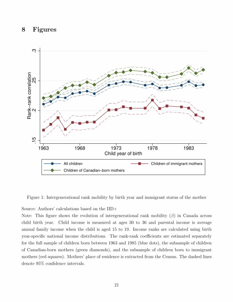
[Insert Figure 1 here.]

Figure 1 shows the evolution of the intergenerational rank mobility coefficient (βt) by year of

8Additional statistics can be found in Appendix Table B2.

6

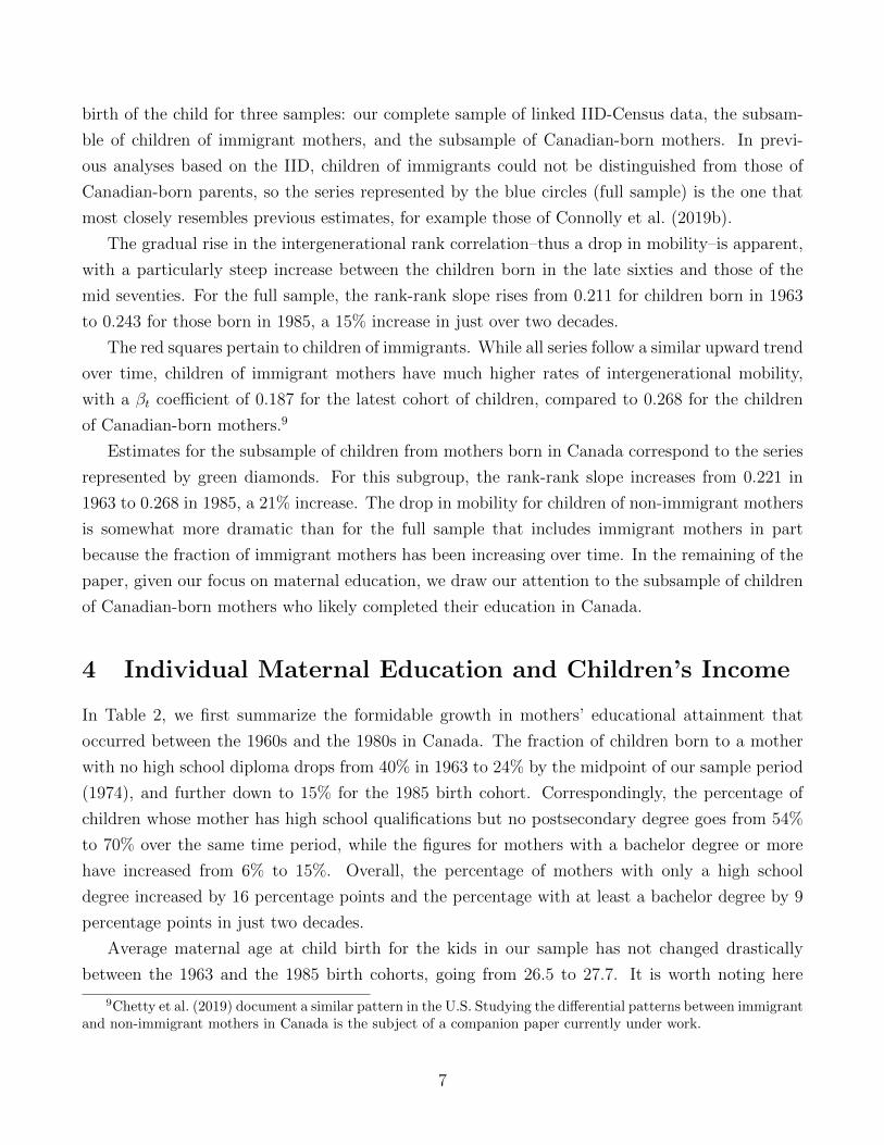
birth of the child for three samples: our complete sample of linked IID-Census data, the subsam-

ble of children of immigrant mothers, and the subsample of Canadian-born mothers. In previ-

ous analyses based on the IID, children of immigrants could not be distinguished from those of

Canadian-born parents, so the series represented by the blue circles (full sample) is the one that

most closely resembles previous estimates, for example those of Connolly et al. (2019b).

The gradual rise in the intergenerational rank correlation–thus a drop in mobility–is apparent,

with a particularly steep increase between the children born in the late sixties and those of the

mid seventies. For the full sample, the rank-rank slope rises from 0.211 for children born in 1963

to 0.243 for those born in 1985, a 15% increase in just over two decades.

The red squares pertain to children of immigrants. While all series follow a similar upward trend

over time, children of immigrant mothers have much higher rates of intergenerational mobility,

with a βt coefficient of 0.187 for the latest cohort of children, compared to 0.268 for the children

of Canadian-born mothers.9

Estimates for the subsample of children from mothers born in Canada correspond to the series

represented by green diamonds. For this subgroup, the rank-rank slope increases from 0.221 in

1963 to 0.268 in 1985, a 21% increase. The drop in mobility for children of non-immigrant mothers

is somewhat more dramatic than for the full sample that includes immigrant mothers in part

because the fraction of immigrant mothers has been increasing over time. In the remaining of the

paper, given our focus on maternal education, we draw our attention to the subsample of children

of Canadian-born mothers who likely completed their education in Canada.

4 Individual Maternal Education and Children’s Income

In Table 2, we first summarize the formidable growth in mothers’ educational attainment that

occurred between the 1960s and the 1980s in Canada. The fraction of children born to a mother

with no high school diploma drops from 40% in 1963 to 24% by the midpoint of our sample period

(1974), and further down to 15% for the 1985 birth cohort. Correspondingly, the percentage of

children whose mother has high school qualifications but no postsecondary degree goes from 54%

to 70% over the same time period, while the figures for mothers with a bachelor degree or more

have increased from 6% to 15%. Overall, the percentage of mothers with only a high school

degree increased by 16 percentage points and the percentage with at least a bachelor degree by 9

percentage points in just two decades.

Average maternal age at child birth for the kids in our sample has not changed drastically

between the 1963 and the 1985 birth cohorts, going from 26.5 to 27.7. It is worth noting here

9Chetty et al. (2019) document a similar pattern in the U.S. Studying the differential patterns between immigrantand non-immigrant mothers in Canada is the subject of a companion paper currently under work.

7

that we consider all children born in those years, not just firstborns. Hence, these numbers may

be influenced by both changes in the timing of fertility as well as in the number of children per

mother.

[Insert Table 2 here.]

To examine the association between income mobility and maternal education, we first re-

estimate rank-rank slopes separately for children of non-immigrant mothers with different levels

of educational attainment. Results are shown in Figure 2. Again, all three series follow a similar

pattern of increasing rank-rank slopes over time, but the rise is much more pronounced for parent-

child pairs in which the mother has no high school diploma. This group consistently displays higher

rank-rank correlations, meaning lower intergenerational mobility, relative to children of mothers

with a high school degree or more. In other words, among children of mothers with no high school

diploma, parental income is more predictive of the child’s income in adulthood than it is among

children of university-educated mothers. In the early years of our sample, most differences in

rank-rank slopes across education groups are not statistically significant at conventional levels.

By the mid seventies, differences between children of mothers with no high school diploma and

children of university-educated mothers become statistically significant at the 5% level. This is

partly because estimates of βt for university-educated mothers become more precise over time with

increasing educational attainment.


To examine potential non-linearities in the intergenerational transmission of income, Table 3

presents quintile transition matrices for three birth cohorts, situated at the beginning, the middle,

and the end of our sample, separately by the mother’s education category. The distribution of

the education categories within a birth cohort are given just above the matrices themselves as

a reminder. The probability to remain in the bottom quintile for children of parents who were

themselves in the bottom quintile has increased in families with mothers who do not have a high

school diploma (top panel). It starts at 33%, and increases to 39% in 1974 then to 42% in 1985,

for an overall increase of 9 percentage points. The probability they reach the third or fourth

quintile of the income distribution has also declined over the period. The overall weight of this

group has decreased over time since mothers are becoming more educated on average, and their

upward mobility has deteriorated. This decline reflects the fact that these children are increasingly

trapped at the bottom of the income distribution and unable to reach higher rungs of the income

distribution. For children of mothers with a high school diploma only (middle panel) and children

of mothers with at least a bachelor degree (bottom panel), we also observe increasing stickiness at

the bottom, from 26% to 32%, and from 27% to 37%, respectively. Poverty traps are becoming

more prevalent in all groups, but the phenomenon is most important for mothers without a high

school diploma. For children of highly educated mothers, the probability to remain at the top of

8

the ladder has declined over the period. This has contributed to an increase in relative mobility

within that group, all the while its share of the population has increased over time as mothers

gained education.


We then document the distribution and evolution of income gaps between children of mothers

with different levels of education. Figure 3 presents a series of binned scatterplots, where each

dot is the mean child percentile rank for a given parental income rank. Rank-rank coefficients

correspond to a linear fit going through those dots.10 There are three panels, one for each broad

maternal education group, and to emphasize changes over time, each panel has two series: one for

the 1963 to 1966 birth cohorts combined (the gray triangles) and one for the 1982 to 1985 birth

cohorts (the blue circles). The size of markers represents the relative weight of each parental income

percentile within education groups. Group-specific rank-rank slopes have increased over time for

each group, but much more so for children of mothers with no high school diploma. These children

are not only more over-represented at the bottom of the parental income distribution in later years,

but their own income ranks have declined dramatically for parental income ranks below the 20th

percentile. Put differently, children of mothers with no high school diploma are increasingly left

behind, suffering a double penalty of now growing up in relatively poorer households and achieving

less upward mobility conditional on parental income being below the 20th percentile.


Figure 4 presents the same data but instead focuses on differences across education groups

within time periods. Again, the size of the markers represents the relative number of observations in

each cell within educational categories. Vertical dashed line indicates the average parental income

rank of each education group. Private intragenerational returns to education (for parents) are

large: the mass is dramatically shifted to the right for university-educated parents, and somewhat

to the left for parents with no high school diploma in 1963-66. For these birth cohorts, the average

parental income percentile is 41 for mothers with no high school diploma, 58 for mothers with at

most a high school degree, and 77 for university-educated mothers. In the later cohorts (1982-85),

the weight is more evenly distributed across parental income percentiles for university-educated

parents given large increases in the number of people completing bachelor degrees. Yet, private

returns to education have increased. The difference in average parental income ranks between

mothers with a bachelor degree and mothers with no high school diploma has increased from 36

to 38 percentiles. This is because the income distribution of parents with no high school diploma

10We focus our analysis on the rank-rank coefficient from a linear regression, a measure that facilitates thecomparisons with other studies, and that summarizes the intergenerational relationship in a compact fashion. Wedo note however that the relationship is not perfectly linear, as is evident from Figure 3. Connolly et al. (2019b)further investigates this non-linearity in the Canadian context. Why non-linearities are more apparent in Canadathan in the United States is a question that merits further research.

9

is now highly concentrated at lower income ranks.


In both periods, the average income ranks of children of educated parents lie above those

from lesser educated families throughout the entire parental income distribution. That is, children

benefit from their parents’ human capital directly, above and beyond what would be expected on

the basis of parental financial resources alone. This is particularly true for families in the bottom 80

percent of the parental income distribution. In contrast, among families at the top of the income

distribution (the top 20% of parental income), children of high school and university educated

mothers have similar outcomes on average. Overall, children of university-educated mothers have

a double advantage: they have access to more financial resources growing up in relatively richer

families, and also achieve higher income ranks conditional on parental income.

Over time, income gaps between children of parents with and without secondary education

have increased in Canada. Increasing income inequality between mothers of different levels of

education as well as decreasing relative intergenerational income mobility have both contributed

to this situation. As a result, children of mothers with no high school diploma are falling further

behind over time.

5 Can National Changes in Maternal Education Account

for Changes in Income Mobility?

In this section, we undertake two accounting analyses to document the role changes in maternal

education may have played in the evolution of intergenerational mobility in Canada.

Firstly, to quantify the mechanical association between maternal education and intergenera-

tional mobility, we ask what the distribution of children outcomes would look like for the 1982-85

cohorts combined had the distribution of maternal education groups across parental income per-

centiles remained at its 1963-66 levels. More precisely, to construct this counterfactual we take the

educational attainment distribution of the mothers of the 1963-66 birth cohorts at each parental

income percentile, and apply those weights to the education-specific child income percentiles of

the 1982-85 cohorts. This is equivalent to both fixing overall educational attainment as well as the

private returns to education (for parents) to their 1963-66 levels. For consistency, we re-center the

resulting distribution of child outcomes to insure that the national mean is 50. 11


Results are shown in Figure 5. The left panel shows the actual rank-rank relationships for

children born in 1963-66 and those born in 1982-85, separately. The right panel plots the actual

11One caveat to keep in mind is that under this naive accounting method the number of children in each percentileof their income distribution need not be equal across percentiles.

10

1982-85 binned scatter plot against the counterfactual distribution, here indicated by red plusses.

The two distributions look fairly similar, with some relatively pronounced deviations from the true

distribution in the bottom half of the parental income distribution. As a result, the rank-rank slope

of the counterfactual distribution is slightly higher than the actual value: 0.281 compared to 0.270.

Our conclusion from this exercise is that the observed increases in maternal education brought

forward a decrease in the rank-rank slope of 0.011, equivalent to 27% of the observed increase of

0.04 points. In other words, the decline in income mobility would have been considerably larger

had changes in parental education not exerted a downward pressure on the rank-rank slope.

Secondly, we examine the evolution of the relationship between child and parent income ranks

conditional on the level of education of the mother. We find that the overall decrease in relative

income mobility between the 1963-66 and 1982-85 birth cohorts is largely accounted for by changes

in rank-rank slopes within education groups. Including education dummies in eq. (1) reduces the

rank-rank slope to 0.203 for the 1963-66 birth cohorts and to 0.249 for the 1982-85 birth cohorts.12

Over time, this conditional rank-rank slope therefore increased by 0.046 points (23%), that is at a

faster rate that the unconditional rank-rank slope did (a 0.04 points (18%) increase from 0.229 to

0.270). This implies that observed changes in the private intergenerational returns to education

and in the fraction of educated parents helped attenuate the overall decrease in relative mobility

over time.

The role of maternal education for income mobility might not be linear. To examine whether

this is the case, we further decompose the unconditional rank-rank relationship into (1) the con-

ditional, within-group, rank-rank coefficient, and (2) additional terms reflecting changes in the

intergenerational returns to maternal education and in educational attainment, separately for high

school completion and bachelor degree completion. More precisely, the unconditional rank-rank

slope can be written

βt = λt +∑j

πj,tRj,t (2)

where λt is the conditional rank-rank coefficient, πj,t is the increase in child outcomes associated

with maternal education level j ∈ {HighSchool, Bachelor} (relative to not completing high school)

conditional on parental income, and Rj,t is the regression coefficient from the projection of maternal

education eit onto xit (the “reverse” of a standard returns to education estimating equation).13


Detailed decomposition results are shown in Table 4, and some components of this decompo-

sition exercise are shown graphically in Appendix Figure A1. We find that for the early cohorts

12Appendix Table A2 shows the rank-rank relationship net of maternal education dummies.13For instance, λt and πj,t are obtained from the “long” regression of children income on parental income and

parental education: yit = at + λtxit +∑

j πj,t1{eit = j}+ εit.

11

(1963-66), the terms πj,tRj,t were positive for both high school completion (0.015) and bachelor

degree completion (0.012). In contrast, for later cohorts (1982-85), the term for high school com-

pletion has effectively shrunk to zero, while it increased to 0.021 for bachelor degree completion.

These results suggest that overall changes in high school completion and in their economic returns

have contributed to slowing down the decrease in intergenerational income mobility. Changes

to bachelor degree completion rates and to their returns pushed in the other direction, further

reinforcing the decrease in mobility. In an accounting sense, this is largely due to the fact that

increases in high school completion rates contribute to reducing the variance of that educational

outcome (moving away from from 50% and towards 100%), whereas increases in bachelor degree

completion rates tend to increase educational variance (moving away from from 0% and towards

50%).

6 Income Mobility and Maternal Education over Time and

Space

In this section, we investigate whether provinces that experienced faster growth in educational

attainment over our study period saw different changes in relative intergenerational mobility. To

do so, we estimate rank-rank slopes βpt separately for children born in different provinces and in

different years. With 10 provinces and 20 birth cohorts, we recover 200 estimates of βpt.14 We plot

these coefficient estimates in Figure A3.

Relative mobility decreases across the board over the two decades we consider, but does so

at different rates across provinces. For instance, Alberta and Saskatchewan saw large increases

in rank-rank slopes βpt between 1963 and 1985–from 0.165 to 0.273 and from 0.172 to 0.339,

respectively–whereas it barely changed in Newfoundland and Labrador (increase from 0.267 to

0.290). There is also substantial cross-sectional variation, with Manitoba exhibiting the lowest

rates of relative mobility in the country over the entire period. The two sources of variation–

over time and across provinces–are quantitatively important. Average differences across provinces

account for 50% of the variance of βpt in our data, and average differences across birth years

account for 30%.

With time-varying provincial estimates of βpt in hand, we then examine the relationship between

relative mobility and aggregate parental education using the following two-way fixed effects model:

βpt = θHSHighSchoolpt + θBABachelorpt + δt + δp + υpt (3)

where HighSchoolpt is the fraction of mothers of children born in province p in year t who com-

14The percentile ranks are still defined over the national distribution of income.

12

pleted high school (including those that further pursued higher education), and Bachelorpt is the

fraction that completed a bachelor degree or more. Hence, θBA represents the incremental effect of

increasing university completion rates, over and above that of increasing high school completion.

We include province fixed effects to account for any fixed institutional and sociological differences

between provinces, as well as birth-year fixed effects to account for common trends in relative

income mobility.

We begin with a visualization of the relationship between relative rank mobility βpt and av-

erage mother’s education. Figure 6 plots in light gray residual mobility against residual parental

education, where circle size indicates the relative number of observations (children) in each cell.

To generate this plot, we first residualize all variables on province and birth-year fixed effects. On

top we show a binscatter plot (in solid blue) of these residuals using optimally chosen bins via

the method developed by Cattaneo et al. (2019). To mimic multiple regression analysis, variables

for one level of education are also residualized on the other level. While a negative relationship

between the fraction of mothers holding a high school diploma and the rank-rank measure is quite

apparent, there is much less of an association with the fraction of mothers holding a bachelor

degree.

Regression estimates of the relationship between aggregate maternal education and relative

mobility are presented in Table 5. Throughout, standard errors are clustered at the province level

to account for serial correlation and we report p-values for wild cluster bootstrap F -tests to address

the issue of a small number of clusters. Column (1) reports OLS results from a specification that

only includes province and birth-year fixed effects as controls. These estimates correspond to the

relationships shown in Figure 6. The point estimate for the coefficient on high school implies that

a one-percentage-point increase in high school completion rates among mothers is associated with

a 0.0058 reduction in the rank-rank income relationship (a 2.3% decrease at the mean). To put this

magnitude in context, the reported coefficient suggests that a one-standard-deviation increase in

high school completion rates reduces the provincial rank-rank slope by 0.0587, roughly equivalent to

the 1985 cross-sectional difference in rank-rank slopes between the seventh-ranked (Newfoundland

and Labrador) and lowest-ranked (Manitoba) province. This relationship is statistically significant

at conventional levels. Consistent with the visual evidence, the coefficient on the share of mothers

with a bachelor degree is small and not statistically significant (-0.0026, s.e. 0.0044). In column (5),

we add province-specific linear time trends. The coefficient on the share of high-school-educated

mothers drops by half but remains statistically significant at the 5% level, whereas the coefficient

on the fraction of bachelor degree holders flips sign and remains not statistically significant.


Next, we examine whether the relationship between relative mobility and maternal education

works through (a) provincial and time differences in the intergenerational private returns to ed-

13

ucation, which govern child income gaps between parental education groups, or via (b) external

effects of aggregate education that shape the transmission of income within education groups.

As a first step, we decompose the variance of the rank-rank slopes βpt to examine whether

differences in relative mobility are mostly due to how individual differences in parental education

affect child outcomes (πHS,ptRHS,pt and πBA,ptRBA,pt), or to differences in the conditional income

rank-rank relationship (λpt). We find that a whopping 94% of the variance in βpt is accounted for

by variation in rank-rank slopes within education groups (λpt).15 That is, differences in mobility

across provinces and over time are largely accounted for by differences in mobility conditional on

individual maternal education. Differences in the intergenerational private returns to education

account for less than 10% of the unconditional variation in βpt.

In columns (2) through (4) of Table 5, we decompose the relationship between aggregate ma-

ternal education and relative mobility by using the components λpt, πHS,ptRHS,pt and πBA,ptRBA,pt

as dependent variables in our two-way fixed effects regressions. By construction, the coefficients

reported in columns (2), (3) and (4) sum up to the ones reported in column (1). Interestingly, both

levels of education are positively associated with conditional rank mobility (negatively associated

with λpt), though the coefficient on fraction of bachelor degree holders is not precisely estimated.

The association between the supply of high-school-educated mothers and the component πHS,ptRHS,pt

(-0.0014, s.e. 0.0005), which captures educational inequality and the private intergenerational re-

turns to a high school education, reinforces the observed relationship with conditional rank mobility

λpt, thereby resulting into a larger total effect on unconditional relative income mobility. That

is, provinces that experienced faster growth in maternal high school completion rates saw slower

deterioration of (unconditional) relative mobility because both their conditional rank-rank slopes

and their intergenerational private returns to high school completion were increasing at a slower

pace. These patterns are qualitatively robust to the inclusion of province-specific linear time trends

(columns (6) to (8)).

In contrast, the fraction of university-educated mothers is positively associated with educational

inequality and private intergenerational returns to college education πBA,ptRBA,pt (0.0016, s.e.

0.0006), which contributes to steepening the unconditional rank-rank relationship. Naturally,

since few mothers have a bachelor degree, any increase in the supply of college-educated mothers

increases the variance in education attainment, and thereby tends to reduce mobility. These

relationships are not significant at conventional levels, however, and the point estimates are not

robust to the inclusion of province-specific time trends.

15Conditional on province and birth-cohort fixed effects, this percentage is 92.8%.

14

7 Conclusion

Just as rising socioeconomic inequalities over the last few decades has garnered attention, so has

now the increasing rate of transmission of those inequalities from one generation to the next. Across

a variety of countries, settings, and measures, children from low socioeconomic backgrounds find it

harder to move up the income distribution in adulthood. While the development of administrative

data, in particular tax data, has allowed researchers to paint very detailed portraits of intergener-

ational mobility and its distribution, few studies have examined the mechanisms driving changes

in mobility. In this paper, we assessed the role maternal education plays in the intergenerational

correlation between parental income rank and child income rank. We leveraged a new data linkage

to present novel facts regarding the interplay between the evolution of rank mobility for cohorts for

children born between 1963 and 1985 in Canada and the educational attainment of their mothers.

First, we show that at the national level, increases in maternal education over time likely have

contributed to slowing down the decrease in relative intergenerational mobility. In particular, a

simple accounting exercise suggests that if the distribution of maternal education across parental

income percentiles had remained at its 1963-66 levels, the observed increase in the rank-rank slope

would have been 27% greater. We also find that the overall decrease in relative income mobility

between the early sixties and the mid eighties is largely accounted for by changes in rank-rank

slopes within maternal education groups. In fact, the conditional rank-rank slope (controlling

for maternal education dummies) increased faster than the unconditional rank-rank slope did,

suggesting that changes in mobility differences between groups have helped attenuate the overall

decrease in relative mobility within education groups.

Second, we leverage variation over time and across provinces to investigate the link between ag-

gregate maternal education and rank mobility. This allows us to move beyond micro relationships

of how more educated parents individually influence their children’s outcomes, and consider aggre-

gate effects of educational attainment on a society (encompassing both the private and the social

returns to education). Here, we treat the unconditional rank-rank slope–an inherently aggregate

measure that characterizes the joint distribution of the parental and child income ranks–as our

dependent variable in a two-way fixed effects regression framework. Our estimates indicate that a

one-percentage-point increase in the share of high school graduates among mothers is associated

with a 0.0058 reduction in the intergenerational rank-rank income relationship (a 2.3% decrease

at the mean). This result is due to maternal high school completion rates being (a) negatively

associated with the conditional (within-group) rank-rank slope and (b) negatively associated with

overall educational inequality, and therefore to how returns to maternal educational are distributed

among children. In fact, increasing high school completion rates have been an equalizing force, as

the fraction of mothers without a high school diploma has shrunk from 40% to 15% in just over

15

two decades. In contrast, we find no evidence that bachelor degree completion among mothers

affects intergenerational income mobility.

Our results are informative in a historical perspective: the generations of parents in our data

lived through a time of rapidly rising educational attainment, a consequence of which appears to

be the mitigation of other forces driving up the intergenerational transmission of socioeconomic

status. Yet our findings can be useful in other settings, including in developing countries which have

yet to experience this rising tide of education, whether it is brought forward through compulsory

schooling laws or other advancements. Our findings also turn the spotlight on a segment of the

current population for whom the opportunities are ever more dire than before: those who leave

school before obtaining a high school diploma. Not only will their own labor market earnings

reflect their low level of education, their children will also on average stay on lower rungs of the

income distribution, suffering a double penalty of lower parental financial resources combined with

lower upward mobility conditional on parental income rank.

This leads us to conclude that policies aimed at increasing the educational attainment of today’s

youth should have the long-run consequence of improving the overall equality of opportunities. A

high school diploma should be seen as a minimum level of education necessary to promote mobility.

Policies that seek to boost school perseverance, particularly for children from low socioeconomic

background, are probably key. Also linked to those are the upstream interventions that take place

in early childhood, such as access to early childhood education, and especially high-quality early

childhood education. Some of the gains of such education policies will be felt more quickly, and

more privately, but our research suggests that there are also longer-term and aggregate benefits

for the society as whole.

16

References

Acemoglu, Daron and Joshua D Angrist (2000). How Large are Human-capital Externalities?

Evidence from Compulsory Schooling Laws. NBER Macroeconomics Annual, 15, 9–59.

Aryal, Gaurab, Manudeep Bhuller, and Fabian Lange (2019). Signaling and Employer Learning

with Instruments. Working Paper 25885. National Bureau of Economic Research.

Becker, Gary S. and Nigel Tomes (1979). An Equilibrium Theory of the Distribution of Income

and Intergenerational Mobility. Journal of Political Economy, 87(6), 1153–1189.

— (1986). Human Capital and the Rise and Fall of Families. Journal of Labor Economics, 4(3,

Part 2), S1–S39. eprint: http://dx.doi.org/10.1086/298118.

Biasi, Barbara (2019). School Finance Equalization Increases Intergenerational Mobility: Evidence

from a Simulated-Instruments Approach. Working Paper 25600. National Bureau of Economic

Research.

Black, Sandra E, Paul J Devereux, Petter Lundborg, and Kaveh Majlesi (2019). Poor Little Rich

Kids? The Role of Nature versus Nurture in Wealth and Other Economic Outcomes and Be-

haviours. The Review of Economic Studies, 87(4), 1683–1725. eprint: https://academic.oup.

com/restud/article-pdf/87/4/1683/33461634/rdz038.pdf.

Black, Sandra E, Paul J Devereux, and Kjell G Salvanes (2005). Why the Apple Doesn’t Fall Far:

Understanding Intergenerational Transmission of Human Capital. American Economic Review,

95(1), 437–449.

Blanden, Jo (2013). Cross-country Rankings in Intergenerational Mobility: A Comparison of Ap-

proaches from Economics and Sociology. Journal of Economic Surveys, 27(1), 38–73.

Blau, Peter M and Otis Dudley Duncan (1967). The American Occupational Structure. New York:

Willey.

Bradbury, Bruce, Miles Corak, Jane Waldfogel, and Elizabeth Washbrook (2015). Too Many Chil-

dren Left Behind: The US Achievement Gap in Comparative Perspective. New York: Russell

Sage Foundation.

Bukodi, Erzsebet and John H Goldthorpe (2013). Decomposing ‘Social Origins’: The Effects of Par-

ents’ Class, Status, and Education on the Educational Attainment of their Children. European

Sociological Review, 29(5), 1024–1039.

Carneiro, Pedro, Costas Meghir, and Matthias Parey (2013). Maternal Education, Home Environ-

ments, and the Development of Children and Adolescents. Journal of the European Economic

Association, 11(suppl 1), 123–160.

Cattaneo, Matias D, Richard K Crump, Max H Farrell, and Yingjie Feng (2019). On Binscatter.

17

http://dx.doi.org/10.1086/298118

https://academic.oup.com/restud/article-pdf/87/4/1683/33461634/rdz038.pdf

https://academic.oup.com/restud/article-pdf/87/4/1683/33461634/rdz038.pdf

Chen, Wen-Hao, Yuri Ostrovsky, and Patrizio Piraino (2017). Lifecycle Variation, Errors-in-variables

Bias and Nonlinearities in Intergenerational Income Transmission: New Evidence from Canada.

Labour Economics, 44, 1–12.

Chetty, Raj, David Grusky, Maximilian Hell, Nathaniel Hendren, Robert Manduca, and Jimmy

Narang (2017). The Fading American Dream: Trends in Absolute Income Mobility since 1940.

Science, 356(6336), 398–406.

Chetty, Raj, Nathaniel Hendren, Maggie R Jones, and Sonya R Porter (Dec. 2019). Race and

Economic Opportunity in the United States: An Intergenerational Perspective. The Quarterly

Journal of Economics. qjz042. eprint: https://academic.oup.com/qje/advance-article-

pdf/doi/10.1093/qje/qjz042/31618473/qjz042.pdf.

Chetty, Raj, Nathaniel Hendren, Patrick Kline, and Emmanuel Saez (2014). Where is the Land

of Opportunity? The Geography of Intergenerational Mobility in the United States. Quarterly

Journal of Economics, 129(4), 1553–1623.

Connolly, Marie, Miles Corak, and Catherine Haeck (2019a). Intergenerational Mobility between

and within Canada and the United States. Journal of Labor Economics, 37(S2), S595–S641.

Connolly, Marie, Catherine Haeck, and David Lapierre (2019b). Social Mobility Trends in Canada:

Going up the Great Gatsby Curve. Working Paper 18-01. Research Group on Human Capital.

Corak, Miles (2006). Do Poor Children Become Poor Adults? Lessons from a Cross Country Com-

parison of Generational Earnings Mobility. In: Research on Economic Inequality. Ed. by John

Creedy and Guyonne Kalb. Vol. 13. Amsterdam: Elsevier.

— (2013). Income Inequality, Equality of Opportunity, and Intergenerational Mobility. Journal of

Economic Perspectives, 27(3), 79–102.

— (2020). The Canadian Geography of Intergenerational Income Mobility. The Economic Journal,

130(631), 2134–2174. eprint: https://academic.oup.com/ej/article-pdf/130/631/2134/

33937507/uez019.pdf.

Corak, Miles and Andrew Heisz (1999). The Intergenerational Earnings and Income Mobility of

Canadian Men: Evidence from Longitudinal Income Tax Data. The Journal of Human Re-

sources, 34(3), 504–533.

Currie, Janet and Enrico Moretti (2003). Mother’s Education and the Intergenerational Transmis-

sion of Human Capital: Evidence from College Openings. The Quarterly Journal of Economics,

118(4), 1495–1532.

Davis, Jonathan and Bhashkar Mazumder (2019). The Decline in Intergenerational Mobility after

1980. Working Paper WP-2017-5. Federal Reserve Bank of Chicago.

Fagereng, Andreas, Magne Mogstad, and Marte Ronning (forthcoming). Why do Wealthy Parents

have Wealthy Children? Journal of Political Economy.

18

https://academic.oup.com/qje/advance-article-pdf/doi/10.1093/qje/qjz042/31618473/qjz042.pdf

https://academic.oup.com/qje/advance-article-pdf/doi/10.1093/qje/qjz042/31618473/qjz042.pdf

https://academic.oup.com/ej/article-pdf/130/631/2134/33937507/uez019.pdf

https://academic.oup.com/ej/article-pdf/130/631/2134/33937507/uez019.pdf

Featherman, David L, F Lancaster Jones, and Robert M Hauser (1975). Assumptions of Social

Mobility Research in the US: The Case of Occupational Status. Social Science Research, 4(4),

329–360.

Goldthorpe, John H (1980). Social Mobility and Class Structure in Modern Britain. Oxford [Eng.]:

Clarendon Press.

— (2013). Understanding–and Misunderstanding–Social Mobility in Britain: The Entry of the

Economists, the Confusion of Politicians and the Limits of Educational Policy. Journal of

Social Policy, 42(3), 431–450.

Goldthorpe, John H and Keith Hope (1974). The Social Grading of Occupations: A New Approach

and Scale. Oxford [Eng.]: Clarendon Press.

Grawe, Nathan D. (2004). Reconsidering the Use of Nonlinearities in Intergenerational Earnings

Mobility as a Test for Credit Constraints. The Journal of Human Resources, 39(3), 813–827.

— (2006). Lifecycle Bias in Estimates of Intergenerational Earnings Persistence. Labour Eco-

nomics, 13(5), 551–570.

Guell, Maia, Jose V Rodrıguez Mora, and Christopher I Telmer (2015). The Informational Content

of Surnames, the Evolution of Intergenerational Mobility, and Assortative Mating. The Review

of Economic Studies, 82(2), 693–735.

Holmlund, Helena, Mikael Lindahl, and Erik Plug (2011). The Causal Effect of Parents’ Schooling

on Children’s Schooling: A Comparison of Estimation Methods. Journal of Economic Litera-

ture, 49(3), 615–51.

Landersø, Rasmus and James J Heckman (2017). The Scandinavian Fantasy: The Sources of Inter-

generational Mobility in Denmark and the US. The Scandinavian journal of economics, 119(1),

178–230.

Lange, Fabian and Robert Topel (2006). The Social Value of Education and Human Capital. In:

Handbook of the Economics of Education. Ed. by Eric A. Hanushek and Finis Welch. Vol. 1.

Elsevier. Chap. 8, pp. 459–509.

Loury, Glenn C. (1981). Intergenerational Transfers and the Distribution of Earnings. Economet-

rica, 49(4), 843–867.

Moretti, Enrico (2004a). Estimating the Social Return to Higher Education: Evidence from Lon-

gitudinal and Repeated Cross-sectional Data. Journal of Econometrics, 121(1-2), 175–212.

— (2004b). Workers’ Education, Spillovers, and Productivity: Evidence from Plant-level Produc-

tion Functions. American Economic Review, 94(3), 656–690.

Olivetti, Claudia and M Daniele Paserman (2015). In the Name of the Son (and the Daughter):

Intergenerational Mobility in the United States, 1850-1940. American Economic Review, 105(8),

2695–2724.

19

Oreopoulos, Philip (2003). The Long-Run Consequences of Living in a Poor Neighborhood. The

Quarterly Journal of Economics, 118(4), 1533–1575.

Oreopoulos, Philip, Marianne E Page, and Ann Huff Stevens (2006). The Intergenerational Effects

of Compulsory Schooling. Journal of Labor Economics, 24(4), 729–760.

Oreopoulos, Philip, Marianne Page, and Ann Huff Stevens (2008). The Intergenerational Effects

of Worker Displacement. Journal of Labor Economics, 26(3), 455–483.

Ostrovsky, Yuri (2017). Doing as Well as One’s Parents?: Tracking Recent Changes in Absolute

Income Mobility in Canada. Economic Insights, Catalogue no. 11-626-X, no. 073. Statistics

Canada.

Pekkarinen, Tuomas, Kjell G Salvanes, and Matti Sarvimaki (2017). The Evolution of Social mM-

bility: Norway during the Twentieth Century. The Scandinavian Journal of Economics, 119(1),

5–33.

Rothstein, Jesse (2019). Inequality of Educational Opportunity? Schools as Mediators of the In-

tergenerational Transmission of Income. Journal of Labor Economics, 37(S1), S85–S123.

Sewell, William H and Robert M Hauser (1975). Education, Occupation, and Earnings. Achieve-

ment in the Early Career. New York: Academic Press.

20

8 Figures.1

5.2

.25

.3R

an

k−

ran

k c

orr

ela

tio

n

1963 1968 1973 1978 1983Child year of birth

All children Children of immigrant mothers

Children of Canadian−born mothers

Figure 1: Intergenerational rank mobility by birth year and immigrant status of the mother

Source: Authors’ calculations based on the IID+

Note: This figure shows the evolution of intergenerational rank mobility (β) in Canada across

child birth year. Child income is measured at ages 30 to 36 and parental income is average

annual family income when the child is aged 15 to 19. Income ranks are calculated using birth

year-specific national income distributions. The rank-rank coefficients are estimated separately

for the full sample of children born between 1963 and 1985 (blue dots), the subsample of children

of Canadian-born mothers (green diamonds), and the subsample of children born to immigrant

mothers (red squares). Mothers’ place of residence is extracted from the Census. The dashed lines

denote 95% confidence intervals.

21

.15

.2.2

5.3

.35

Ra

nk−

ran

k c

orr

ela

tio

n


No high school High school

Bachelor degree

Figure 2: Intergenerational rank mobility by birth year and educational attainment of the mother

Source: Authors’ calculations based on the IID+Note: This figure shows the evolution of intergenerational rank mobility (β) in Canada across childbirth year, separately for three groups based on maternal education. Child income is measured atages 30 to 36 and parental income is average annual family income when the child is aged 15 to 19.Income ranks are calculated using birth year-specific national income distributions. The rank-rankcoefficients are estimated separately for children whose mother has no high school degree (bluedots), children whose mother has a high school diploma but no bachelor degree (red squares), andchildren whose mother has at least a bachelor degree (green diamonds). In all cases, the sampleis restricted to Canadian-born mothers. Mothers’ education is extracted from the Census. Thedashed lines denote 95% confidence intervals.

22

Slope 63−66 = 0.218

Slope 82−85 = 0.303

20

30

40

50

60

70

0 20 40 60 80 100Percentile of parental income

when child aged 15 to 19

No high school

Slope 63−66 = 0.193

Slope 82−85 = 0.239

20

30

40

50

60

70



High school

Slope 63−66 = 0.206

Slope 82−85 = 0.246

20

30

40

50

60

70



Bachelor

Me

an

ch

ild p

erc

en

tile

at

ag

e 3

0 t

o 3

6

1963−66 Birth cohorts 1982−85 Birth cohorts

Figure 3: Intergenerational rank mobility by maternal education, 1963-66 and 1982-85 birth cohorts

Source: Authors’ calculations based on the IID+Note: This figure shows the rank-rank relationship between child and parental income, separatelyfor two birth cohorts (1963-66 and 1982-85) and three levels of maternal educational attainment.Each point in this graph represents the mean child percentile rank for a given parental incomerank, where child income is measured at ages 30 to 36 and parental income is average annual familyincome when the child is aged 15 to 19. The markers are weighted using the number of childrenin each cell. The slopes are coefficients from linear rank-rank regressions.

23

20

30

40

50

60

70



1963−66

20

30

40

50

60

70



1982−85

Me

an

ch

ild p

erc

en

tile

at

ag

e 3

0 t

o 3

6

No high school High school Bachelor

Figure 4: Intergenerational rank mobility by maternal education, 1963-66 and 1982-85 birth cohorts

Source: Authors’ calculations based on the IID+Note: This figure shows the rank-rank relationship between child and parental income, separatelyfor three levels of maternal educational attainment and two birth cohorts (1963-66 and 1982-85).Each point in this graph represents the mean child percentile rank for a given parental incomerank, where child income is measured at ages 30 to 36 and parental income is average annual familyincome when the child is aged 15 to 19. The markers are weighted using the number of childrenin each cell. The dashed vertical lines indicate the average parental income rank of each maternaleducation group.

24

Slope 63−66 = 0.229

Slope 82−85 = 0.27

20

30

40

50

60

70



1963−66 Birth cohorts 1982−85 Birth cohorts

Slope counterfactual = 0.281

Slope 82−85 = 0.27

20

30

40

50

60

70



1982−85 Counterfactual 1982−85 Birth cohorts

Me

an

ch

ild p

erc

en

tile

at

ag

e 3

0 t

o 3

6

Figure 5: Intergenerational rank mobility, 1963-66 and 1982-85 birth cohorts and counterfactual

Source: Authors’ calculations based on the IID+Note: This figure shows actual and counterfactual rank-rank relationships between child andparental income. Each point in this graph represents the mean child percentile rank for a givenparental income rank, where child income is measured at ages 30 to 36 and parental income isaverage annual family income when the child is aged 15 to 19. The slopes are from linear rank-rankregressions. The counterfactual series is constructed by taking a weighted average of child incomeranks across maternal education categories within each parental income percentile, applying 1963-66 maternal education weights to 1982-85 child outcomes. The series is then re-centered so thatthe overall average child income rank is equal to 50.

25

−.1

−.0

50

.05

.1R

an

k−

ran

k c

oe

ffic

ien

t β (

resid

ua

lize

d)

−4 −2 0 2 4 6Fraction of mothers with high school diploma

(residualized)

−.1

−.0

50

.05

.1R

an

k−

ran

k c

oe

ffic

ien

t β (

resid

ua

lize

d)

−4 −2 0 2 4 6Fraction of mothers with bachelor degree

(residualized)

Figure 6: Intergenerational rank mobility and maternal education across time and space

Source: Authors’ calculations based on the IID+Note: This figure shows in light grey a scatter plot of relative income mobility (βpt) at the province-by-birth year level, against the average education of mothers in each cell. Variables on both axesare first residualized from province and birth year fixed effects, and each education dummy isalso residualized on each other. The size of markers reflects the number of children in each cell.Blue dots show a binscatter of the underlying data, where bins are selected using the procedureproposed by Cattaneo et al. (2019) and implemented using the associated binsreg Stata command.

26

9 Tables

Table 1: Intergenerational Income Database Cohorts

Birth years IID weighted Share linkedcount to Census

1963 to 1966 1,566,240 0.621967 to 1970 1,555,280 0.631972 to 1975 1,474,140 0.681977 to 1980 1,557,800 0.691982 to 1985 1,633,270 0.69

Source: Authors’ calculations based on the IID+Note: This table shows the weighted counts of children by group of birth years. The weightedcounts use the IID weights. The last column shows the share of families for which mothers weresuccessfully matched to at least one of the six Censuses between 1991 and 2016.

27

Table 2: Maternal Education and Mother’s Age at Birth by Child Birth Cohort

Maternal educational attainmentNo high school High school Bachelor

Birth cohort (%) (%) (%) Mother’s age at birth

1963 40 54 6 26.51964 40 54 6 26.61965 39 55 6 26.51966 37 56 6 26.41967 35 58 7 26.21968 33 59 8 26.11969 32 60 8 26.21970 30 62 9 26.11972 26 64 10 26.11973 25 65 10 26.11974 24 66 10 26.11975 22 67 11 26.21977 20 68 12 26.61978 19 68 12 26.71979 19 69 13 26.81980 18 69 13 26.81982 16 69 15 27.21983 16 69 14 27.31984 16 70 15 27.41985 15 70 15 27.7

Variation1963 to 1985 −25 +16 +9 +1.2

Source: Authors’ calculations based on the IID+Note: These statistics are computed using the IID weights. Weighted number of observations is3,051,485.

28

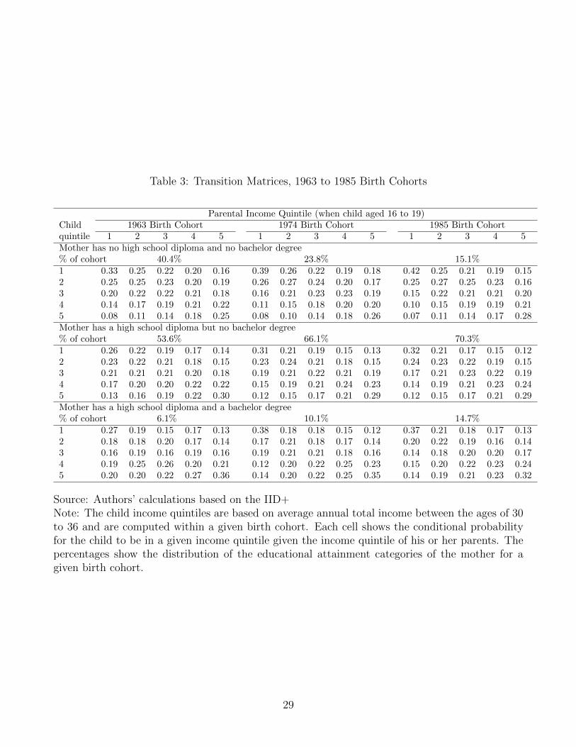
Table 3: Transition Matrices, 1963 to 1985 Birth Cohorts

Parental Income Quintile (when child aged 16 to 19)Child 1963 Birth Cohort 1974 Birth Cohort 1985 Birth Cohortquintile 1 2 3 4 5 1 2 3 4 5 1 2 3 4 5Mother has no high school diploma and no bachelor degree% of cohort 40.4% 23.8% 15.1%1 0.33 0.25 0.22 0.20 0.16 0.39 0.26 0.22 0.19 0.18 0.42 0.25 0.21 0.19 0.152 0.25 0.25 0.23 0.20 0.19 0.26 0.27 0.24 0.20 0.17 0.25 0.27 0.25 0.23 0.163 0.20 0.22 0.22 0.21 0.18 0.16 0.21 0.23 0.23 0.19 0.15 0.22 0.21 0.21 0.204 0.14 0.17 0.19 0.21 0.22 0.11 0.15 0.18 0.20 0.20 0.10 0.15 0.19 0.19 0.215 0.08 0.11 0.14 0.18 0.25 0.08 0.10 0.14 0.18 0.26 0.07 0.11 0.14 0.17 0.28Mother has a high school diploma but no bachelor degree% of cohort 53.6% 66.1% 70.3%1 0.26 0.22 0.19 0.17 0.14 0.31 0.21 0.19 0.15 0.13 0.32 0.21 0.17 0.15 0.122 0.23 0.22 0.21 0.18 0.15 0.23 0.24 0.21 0.18 0.15 0.24 0.23 0.22 0.19 0.153 0.21 0.21 0.21 0.20 0.18 0.19 0.21 0.22 0.21 0.19 0.17 0.21 0.23 0.22 0.194 0.17 0.20 0.20 0.22 0.22 0.15 0.19 0.21 0.24 0.23 0.14 0.19 0.21 0.23 0.245 0.13 0.16 0.19 0.22 0.30 0.12 0.15 0.17 0.21 0.29 0.12 0.15 0.17 0.21 0.29Mother has a high school diploma and a bachelor degree% of cohort 6.1% 10.1% 14.7%1 0.27 0.19 0.15 0.17 0.13 0.38 0.18 0.18 0.15 0.12 0.37 0.21 0.18 0.17 0.132 0.18 0.18 0.20 0.17 0.14 0.17 0.21 0.18 0.17 0.14 0.20 0.22 0.19 0.16 0.143 0.16 0.19 0.16 0.19 0.16 0.19 0.21 0.21 0.18 0.16 0.14 0.18 0.20 0.20 0.174 0.19 0.25 0.26 0.20 0.21 0.12 0.20 0.22 0.25 0.23 0.15 0.20 0.22 0.23 0.245 0.20 0.20 0.22 0.27 0.36 0.14 0.20 0.22 0.25 0.35 0.14 0.19 0.21 0.23 0.32

Source: Authors’ calculations based on the IID+Note: The child income quintiles are based on average annual total income between the ages of 30to 36 and are computed within a given birth cohort. Each cell shows the conditional probabilityfor the child to be in a given income quintile given the income quintile of his or her parents. Thepercentages show the distribution of the educational attainment categories of the mother for agiven birth cohort.

29

Table 4: Decomposition of Rank Mobility Changes

Panel A: Intergenerational mobility terms 1963-66 1982-85 Change % ChangeUnconditional rank-rank slope (β) 0.229 0.269 0.040 18%Conditional rank-rank slope (λ) 0.203 0.249 0.046 23%High school returns: πHS ×RHS 0.015 0.000 -0.015 -103%RHS 0.003 0.000 -0.004 -103%πHS 4.217 4.815 0.599 14%

Bachelor returns: πBA ×RBA 0.012 0.021 0.010 84%RBA 0.002 0.004 0.002 101%πBA 6.390 5.825 -0.565 -9%

Panel B: Average parental income percentile by educationNo high school diploma 40.512 33.857 -6.655 -16%High school diploma 57.611 51.817 -5.795 -10%Bachelor degree 76.844 72.106 -4.738 -6%Panel C: Maternal educational attainment (shares)No high school diploma 0.388 0.159 -0.230 -59%High school diploma 0.549 0.695 0.146 27%Bachelor degree 0.063 0.146 0.084 133%

Source: Authors’ calculations based on the IID+Note: This table presents estimates of rank mobility parameters separately for the 1963-66 and1982-85 birth cohorts. In Panel A, the conditional rank-rank slope is obtained by regressing childincome ranks on parental income ranks, controlling for maternal education dummies. We alsoreport the values of terms associated with returns to maternal high school education (πHS ×RHS)and with returns to maternal bachelor degree completion (πBA×RBA), where πj is the increase inchild outcomes associated with maternal education level j (relative to not completing high school)conditional on parental income, and Rj is the regression coefficient from the projection of maternaleducation onto parental income. In Panel B, we report average parental income ranks for eachcategory of maternal education, and in Panel C we report fractions of children whose mother fallsinto given education groups.

30

Table 5: Association Between Maternal Educational Attainment and Relative Mobility

Dependent variable:Uncond. Cond. High school Bachelor Uncond. Cond. High school Bachelor

rank-rank rank-rank returns returns rank-rank rank-rank returns returnsslope slope slope slope(β) (λ) (πHSRHS) (πBARBA) (β) (λ) (πHSRHS) (πBARBA)(1) (2) (3) (4) (5) (6) (7) (8)

Maternal education% high school diploma -0.0058 -0.0045 -0.0014 0.0001 -0.0028 -0.0024 -0.0008 0.0005

(0.0014) (0.0012) (0.0005) (0.0001) (0.0009) (0.0012) (0.0005) (0.0004)[0.0000] [0.0090] [0.0020] [0.1892] [0.0190] [0.1592] [0.0290] [0.3083]

% bachelor degree -0.0026 -0.0054 0.0012 0.0016 0.0014 0.0015 0.0008 -0.0009(0.0044) (0.0042) (0.0007) (0.0006) (0.0038) (0.0030) (0.0008) (0.0012)[0.6176] [0.2753] [0.2292] [0.1672] [0.8028] [0.7257] [0.3373] [0.5175]

N 200 200 200 200 200 200 200 200Adjusted R2 0.840 0.827 0.790 0.627 0.910 0.900 0.822 0.689Mean dependent variable 0.252 0.227 0.021 0.005 0.252 0.227 0.021 0.005ControlsProvince fixed effects x x x x x x x xBirth-year fixed effects x x x x x x x xProvince-specific linear trends x x x x

Source: Authors’ calculations based on the IID+Note: This table reports OLS regression estimates of the relationship between intergenerational income mobility parameters andmaternal education. One observation is a province-by-birth year cell, and observations are weighted by the number of childrenin each cell. The dependent variable is the unconditional rank-rank slope in columns (1) and (5), the conditional rank-rankslope in columns (2) and (6), the component associated with returns to high school completion in columns (3) and (7), and thecomponent associated with returns to bachelor degree completion in columns (4) and (8). All models include province fixedeffects and birth-year fixed effects. Columns (5) through (8) further include province-specific linear time trends. Standard errorsare clustered at the province level and reported in parentheses. p-values from wild cluster bootstrap F -tests are reported insquare brackets.

31

A Appendix Figures

Conditional slope = 0.203

πBA = 6.39

πHS = 4.22

20

30

40

50

60

70



1963−66


πBA = 5.83

πHS = 4.82

20

30

40

50

60

70



1982−85

Me

an

ch

ild p

erc

en

tile

at

ag

es 3

0 t

o 3

6

No high school High school Bachelor

Figure A1: Intergenerational rank mobility within maternal education groups, 1963-66 and 1982-85

birth cohorts


Note: Each point in this graph represents the mean child percentile rank for a given parental

income rank, where child income is measured at ages 30 to 36 and parental income is average

annual family income when the child is aged 15 to 19. The markers are weighted using the number

of children in each cell. The slopes are coefficients from linear rank-rank regressions of child income

rank on parent income rank controlling for parental education dummies. The values of πHS and

πBA are the estimated coefficients on those dummy variables.

32

Unconditional slope = 0.229


20

30

40

50

60

70



1963−66

Unconditional slope = 0.269


20

30

40

50

60

70



1982−85

Me

an

ch

ild p

erc

en

tile

at

ag

es 3

0 t

o 3

6

Unconditional Conditional

Figure A2: Intergenerational rank mobility within maternal education groups, 1963-66 and 1982-85

birth cohorts


Note: This figure shows the rank-rank relationship between child and parental income ranks. The

conditional series are constructed by regressing child income ranks on dummies for each parental

income percentile, controlling for maternal education dummies. The blue dots show the values of

those regression coefficients, which have been re-centered so that the overall average child income

rank is equal to 50. Child income is measured at ages 30 to 36 and parental income is average

annual family income when the child is aged 15 to 19. The markers are weighted using the number

of children in each cell. The unconditional slopes are coefficients from linear rank-rank regressions

of child income rank on parent income rank, and the conditional slopes are coefficients from

linear rank-rank regressions of child income rank on parent income rank controlling for maternal

education dummies.

33

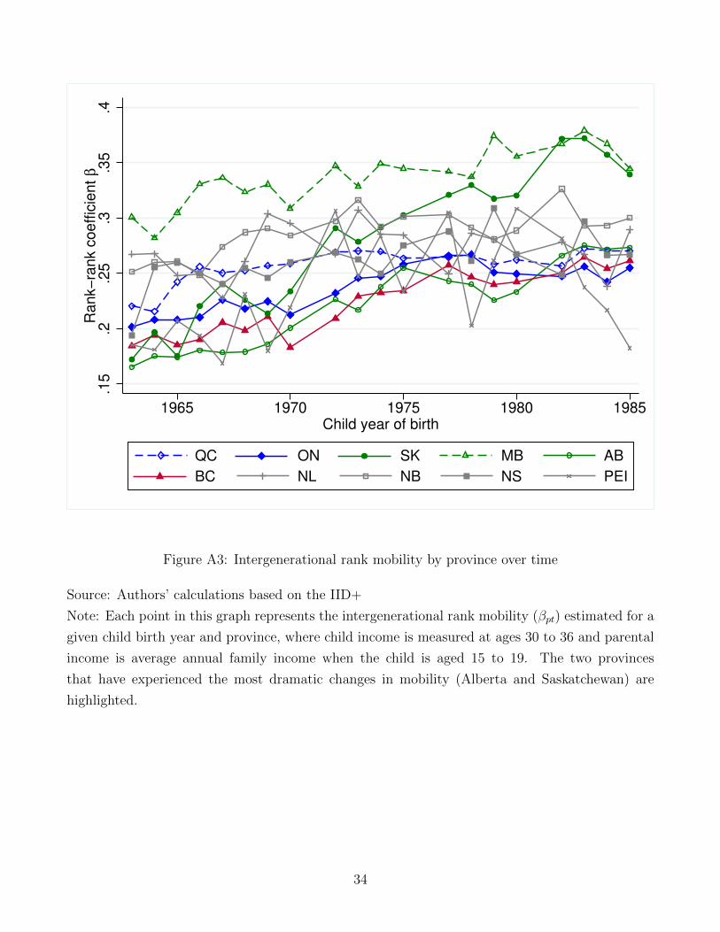
.15

.2.2

5.3

.35

.4R

an

k−

ran

k c

oe

ffic

ien

t β


QC ON SK MB AB

BC NL NB NS PEI

Figure A3: Intergenerational rank mobility by province over time


Note: Each point in this graph represents the intergenerational rank mobility (βpt) estimated for a

given child birth year and province, where child income is measured at ages 30 to 36 and parental

income is average annual family income when the child is aged 15 to 19. The two provinces

that have experienced the most dramatic changes in mobility (Alberta and Saskatchewan) are

highlighted.

34

B Data Appendix

B.1 IID and IID+

The IID+ includes 68 percent of the families originally present in the IID, when only the match

to the mother is performed. It consists of more than four million parent-child pairs, forming a

nationally-representative sample of individuals born from 1963 to 1985.

Table B1: Descriptive Statistics

Variable Mean Std. Dev.Child is male 0.513 0.500Child is female 0.487 0.500Child total income (constant 2016 $)Ages 25 to 29 36,800 28,620Ages 27 to 31 41,800 36,290Ages 30 to 34 48,000 79,060Ages 30 to 36 49,600 80,020Parental total income (constant 2016 $)When child aged 15 to 19 89,500 119,880When child aged 10 to 19 85,700 92,500When mother aged 40 to 49 90,500 96,150When mother aged 45 to 49 97,400 121,020Single mother at time of IID link 0.157 0.363Mother’s age at birth 26.6 5.240Mother’s educational attainmentMother has a high school diploma 0.745 0.436Mother has a bachelor degree 0.106 0.308

Source: Authors’ calculations based on the IID+Note: These statistics are computed using the IID weights. Weighted number of observations is3,051,485. Some variables are based on a slightly smaller number of observations due to missingvalues.

35

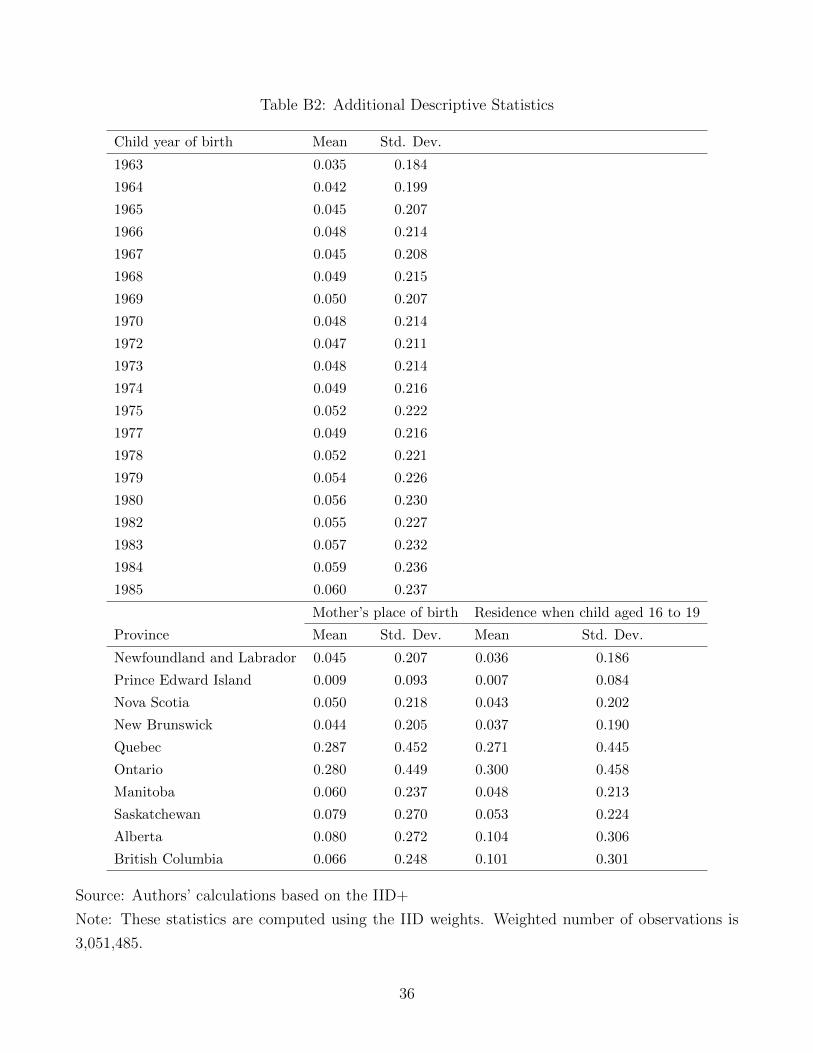
Table B2: Additional Descriptive Statistics

Child year of birth Mean Std. Dev.

1963 0.035 0.184

1964 0.042 0.199

1965 0.045 0.207

1966 0.048 0.214

1967 0.045 0.208

1968 0.049 0.215

1969 0.050 0.207

1970 0.048 0.214

1972 0.047 0.211

1973 0.048 0.214

1974 0.049 0.216

1975 0.052 0.222

1977 0.049 0.216

1978 0.052 0.221

1979 0.054 0.226

1980 0.056 0.230

1982 0.055 0.227

1983 0.057 0.232

1984 0.059 0.236

1985 0.060 0.237

Mother’s place of birth Residence when child aged 16 to 19

Province Mean Std. Dev. Mean Std. Dev.

Newfoundland and Labrador 0.045 0.207 0.036 0.186

Prince Edward Island 0.009 0.093 0.007 0.084

Nova Scotia 0.050 0.218 0.043 0.202

New Brunswick 0.044 0.205 0.037 0.190

Quebec 0.287 0.452 0.271 0.445

Ontario 0.280 0.449 0.300 0.458

Manitoba 0.060 0.237 0.048 0.213

Saskatchewan 0.079 0.270 0.053 0.224

Alberta 0.080 0.272 0.104 0.306

British Columbia 0.066 0.248 0.101 0.301


Note: These statistics are computed using the IID weights. Weighted number of observations is

3,051,485.

36

Differences in rank mobility measured using the IID or the IID+ are negligible. When child

income is measured between the ages of 30 to 36, and parental income is measured when the child

is 15 to 19 years old, the largest difference we observe on the rank-rank slope using the IID versus

the IID+ is 0.0043 in absolute value (less that 2% of the average value) and the smallest is 0.0003.

If child income is instead measured between the ages of 27 to 31 inclusively, the largest difference

is 0.0038 in absolute value and the smallest is 0.00035. Clearly, interpretation of results using the

IID+ leads to extremely similar conclusions to those using the IID. The risk of bias from using

the restricted sample, the IID+, for which information on the mother is available in one of the

Censuses, is therefore minimal when studying rank mobility.

B.2 Definition of maternal education

In this paper, we use two dummy variables to define the education status of mothers. First we

determine whether the mother has obtained a high school diploma, and then we indicate whether

the mother has completed at least a bachelor degree. Below, we document how these two dummies

are coded across different Census waves.

HIGH SCHOOL DIPLOMA DUMMY

The high school (HS) dummy is constructed using two variables: HDGREE in 2006, 2011 and

2016, and HLOSP in 1991, 1996 and 2001. The fields for these variables are listed below. In all

cases, the education variables are only populated for people 15 years of age and over, excluding

institutional residents.

The HS dummy is set equal to one under the following conditions:

• Census 2016: HDGREE > 1 & < 14

• NHS 2011: HDGREE > 1 & < 14

• Census 2006: HDGREE > 1 & < 14

• Census 2001: HLOSP > 3 & < 15

• Census 1996: HLOSP > 3 & < 15

• Census 1991: HLOSP > 3 & < 15

BACHELOR DEGREE COMPLETED DUMMY

The bachelor (BA) dummy is constructed using the same two variables, HDGREE in 2006,

2011 and 2016, and HLOSP in 1991, 1996 and 2001. The bachelor dummy is set equal to one

under the following conditions :

37

• Census 2016: HDGREE > 8 & < 14

• NHS 2011: HDGREE > 8 & < 14

• Census 2006: HDGREE > 8 & < 14

• Census 2001: HLOSP > 10 & < 15

• Census 1996: HLOSP > 10 & < 15

• Census 1991: HLOSP > 10 & < 15

The categories of HDGREE and HLOSP are listed below.

B.2.1 Dataset: 2016 Census of Population

Variable HDGREE: Education: Highest certificate, diploma or degree

Values Categories

1 No certificate, diploma or degree

2 Secondary (high) school diploma or equivalency certificate

3 Trades certificate or diploma other than Certificate of Appr

4 Certificate of Apprenticeship or Certificate of Qualification

5 Program of 3 months to less than 1 year (College, CEGEP and

6 Program of 1 to 2 years (College, CEGEP and other non-university

7 Program of more than 2 years (College, CEGEP and other non-university

8 University certificate or diploma below bachelor level

9 Bachelor’s degree

10 University certificate or diploma above bachelor level

11 Degree in medicine, dentistry, veterinary medicine or optometry

12 Master’s degree

13 Earned doctorate

88 Not available

99 Not applicable

38

B.2.2 Datasets: 2011 National Household Survey and 2006 Census of Population

Variable HDGREE: Education: Highest certificate, diploma or degree

Values Categories

1 None

2 High school graduation certificate or equivalency certificat

3 Other trades certificate or diploma

4 Registered apprenticeship certificate

5 College, CEGEP or other non-university certificate or diploma



8 University certificate or diploma below bachelor level

9 Bachelor’s degree

10 University certificate or diploma above bachelor level

11 Degree in medicine, dentistry, veterinary medicine or optometry

12 Master’s degree

13 Earned doctorate degree

88 Not available

99 Not applicable

B.2.3 Datasets: 1991, 1996 and 2001 Census of Population

Variable HLOSP: HIGHEST LEVEL OF SCHOOLING

Values Categories

1 Less than Grade 5

2 Grades 5 to 8

3 Grades 9 to 13

4 Secondary - high school graduation certificate

5 Trades certificate or diploma

6 College: Without trades or college certificate or diploma

7 College: With trades certificate or diploma

8 College: With college certificate or diploma

9 University: Without certificate, diploma or degree

10 University: With university or college certificate or diploma

11 University: With bachelor or first professional degree

12 University: With certificate or diploma above bachelor level

39

13 University: With master’s degree[s]

14 University: With earned doctorate

98 Not available

99 Not applicable

40

Parental Education and the Rising Transmission of Income ...

Documents

Transcript of Parental Education and the Rising Transmission of Income ...