Parametrized inversion framework for proppant volume in a hydraulically fractured reservoirLindsey J. Heagy⇤, A. Rowan Cockett, Douglas W. Oldenburg, UBC Geophysical Inversion Facility, University ofBritish Columbia

SUMMARY

Hydraulic fracturing is an important technique to allow mobi-lization of hydrocarbons in tight reservoirs. Sand or ceramicproppant is pumped into the fractured reservoir to ensure frac-tures remain open and permeable after the hydraulic treatment.As such, the distribution of proppant is a controlling factoron where the reservoir is permeable and can be effectivelydrained. Methods to monitor the fracturing process, such astiltmeters or microseismic, are not sensitive to proppant distri-butions in the subsurface after the fracturing treatment is com-plete (Cipolla and Wright, 2000).An electrically conductive proppant could create a signifi-cant physical property contrast between the propped region ofthe reservoir and the host rock. Electromagnetic geophysicalmethods can be used to image this property (Heagy and Olden-burg, 2013). However, traditional geophysical inversions arepoorly constrained, requiring a-priori information to be in-corporated through known electrical properties. We examinea strategy to invert directly for the proppant volume using aparametrization of electrical conductivity in terms of proppantdistribution within the reservoir.

INTRODUCTION

Many of the remaining oil and gas reserves are trapped tightlyin low permeability rock formations. These hydrocarbons aredifficult to extract because of the limited availability of path-ways through which they can flow. Pathways can be opened upusing hydraulic fracturing followed by proppant, which staysin the fractures to keep the newly created pathways open (Mont-gomery et al., 2010).

The distribution of proppant is a determining factor on whichregions of the reservoir can be effectively drained. As a result,knowledge of the proppant distribution could provide valuableinsight into decisions regarding well placement, well spacing,and fracture completion strategies (Montgomery et al., 2010;King, 2010). Currently no technique provides a satisfactorymethod of delineating the distribution of proppant within ahydraulically fractured reservoir (Cipolla and Wright, 2000).Electromagnetic (EM) geophysical techniques have been usedto distinguish and delineate electrically conductive regions fromresistive backgrounds. A large conductivity contrast betweenthe propped region of the reservoir and the host rock is nec-essary for data sensitivity in EM geophysics. An electricallyconductive proppant could be created by using a conductivecoating on the particles or using conductive particles. The con-trast of this proppant against the background provides a targetthat can be characterized using EM methods. This requires aproper survey to collect EM data and a methodology to invertthese data.

Traditionally, the inverse problem is approached by consider-

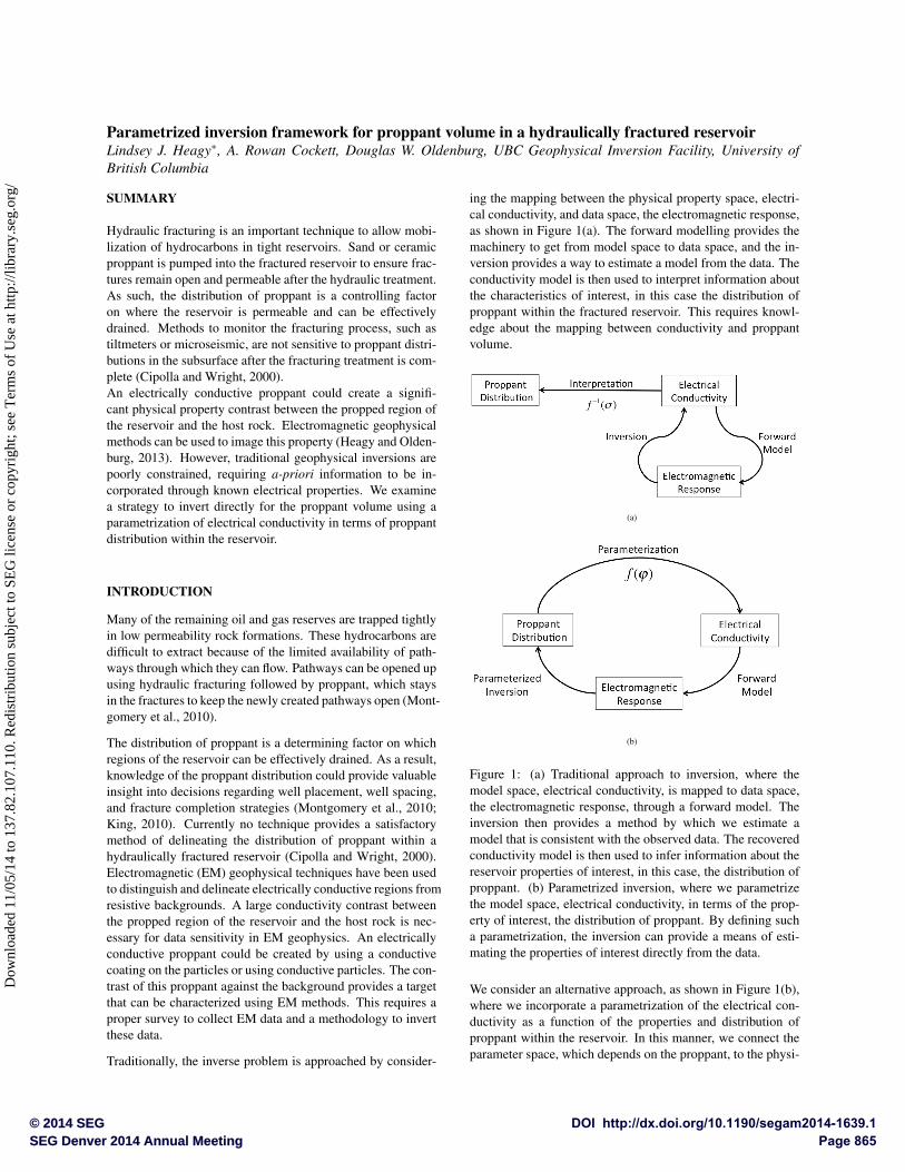
ing the mapping between the physical property space, electri-cal conductivity, and data space, the electromagnetic response,as shown in Figure 1(a). The forward modelling provides themachinery to get from model space to data space, and the in-version provides a way to estimate a model from the data. Theconductivity model is then used to interpret information aboutthe characteristics of interest, in this case the distribution ofproppant within the fractured reservoir. This requires knowl-edge about the mapping between conductivity and proppantvolume.

(a)

(b)

Figure 1: (a) Traditional approach to inversion, where themodel space, electrical conductivity, is mapped to data space,the electromagnetic response, through a forward model. Theinversion then provides a method by which we estimate amodel that is consistent with the observed data. The recoveredconductivity model is then used to infer information about thereservoir properties of interest, in this case, the distribution ofproppant. (b) Parametrized inversion, where we parametrizethe model space, electrical conductivity, in terms of the prop-erty of interest, the distribution of proppant. By defining sucha parametrization, the inversion can provide a means of esti-mating the properties of interest directly from the data.

We consider an alternative approach, as shown in Figure 1(b),where we incorporate a parametrization of the electrical con-ductivity as a function of the properties and distribution ofproppant within the reservoir. In this manner, we connect theparameter space, which depends on the proppant, to the physi-

Page 865SEG Denver 2014 Annual MeetingDOI http://dx.doi.org/10.1190/segam2014-1639.1© 2014 SEG

Dow

nloa

ded

11/0

5/14

to 1

37.8

2.10

7.11

0. R

edis

trib

utio

n su

bjec

t to

SEG

lice

nse

or c

opyr

ight

; see

Ter

ms

of U

se a

t http

://lib

rary

.seg

.org

/

Inversion for Proppant Volume

cal property space, electrical conductivity, through a parametriza-tion. As a result, we provide a mapping from the parame-ter space to the data space. This can be exploited in the in-verse problem, where we are now able to invert directly for theproperty of interest, namely the distribution of proppant in thereservoir.

We tackle this problem in three stages. First, we characterizethe physical properties of a doped fractured reservoir. The goalof this characterization is to provide a mapping that connectsthe parameter space of interest, the proppant distribution, to thephysical property space, the bulk electrical conductivity. Next,we choose a geophysical survey which provides data sensi-tive to the electrical conductivity variations at the scale of thereservoir. Finally, we design an inversion framework whichconnects the observed data back to a distribution of proppantwithin the reservoir. We then show the utility of this approachusing a simple linear inverse problem.

PARAMETRIZATION

We are interested in characterizing the impact of includingelectrically conductive proppant in a fractured volume of areservoir using a relationship of the form

s = f (j) (1)

where s is the parametrized electrical conductivity, j 2 [0,1]is the volume fraction of proppant in a given region of thereservoir, and f is a parametrization that maps from j-spaceto s -space. This parametrization may be derived empiricallyfrom lab measurements or through an upscaling procedure suchas effective medium theory (Bruggeman, 1935; Torquato, 2002;Shafiro and Kachanov, 2000; Berryman and Hoversten, 2013).It is important to note that, in general, the parametrization maybe such that the inverse j = f�1(s) is not well defined. Thisinverse mapping is necessary in the traditional approach to in-version, as outlined in Figure 1(a). In such a scenario, mappingfrom electrical conductivity to proppant distribution requiressolving a separate inverse problem with distinct regularization.Requiring the solution of two inverse problems creates a dis-connect between regularization on the electrical conductivityand regularization on the proppant distribution. In this case,it may be unclear how regularization on conductivity impactsthe characteristics of the proppant model. We find that solvingan intermediate inverse problem for electrical conductivity isunsatisfying and potentially problematic.

For this paper, we consider the propped region of the reservoirto be a two-phase material, composed of the host reservoir,with conductivity s0, and proppant, with conductivity s1. As-suming that the electrical conductivity of the proppant is suf-ficiently large compared to that of any injected fluid, we canneglect the contribution of the electrical conductivity of thefluid.

For the parametrization, we express the effective conductiv-ity of a propped region of a reservoir using self-consistent ef-fective medium theory (Bruggeman, 1935; Torquato, 2002),namely

(1�j)(s �s0)R(0) +j(s �s1)R(1) = 0. (2)

When we consider the effective conductivity of the fracturedrock to be isotropic the factor R(i) is given by

R(i) =

1+

13

si �ss

��1. (3)

Note that if we were to consider an anisotropic conductivity,the R would instead be a matrix (see for example Shafiro andKachanov (2000); Berryman and Hoversten (2013); Torquato(2002)).

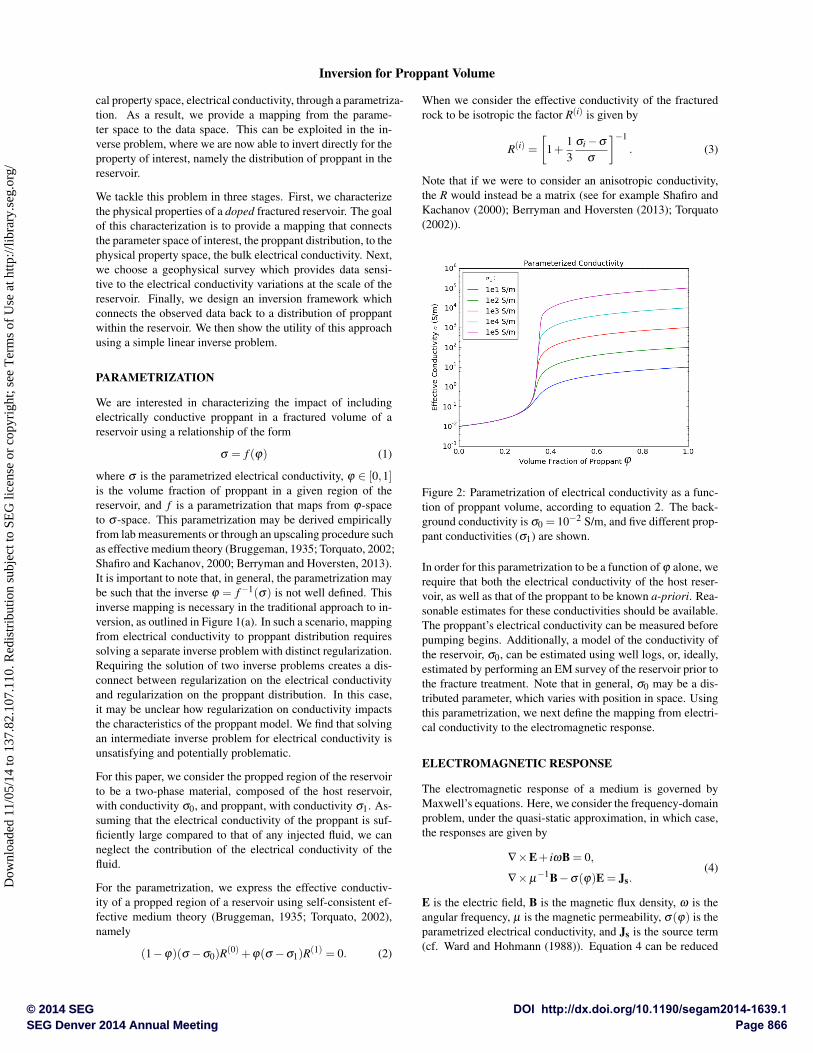
Figure 2: Parametrization of electrical conductivity as a func-tion of proppant volume, according to equation 2. The back-ground conductivity is s0 = 10�2 S/m, and five different prop-pant conductivities (s1) are shown.

In order for this parametrization to be a function of j alone, werequire that both the electrical conductivity of the host reser-voir, as well as that of the proppant to be known a-priori. Rea-sonable estimates for these conductivities should be available.The proppant’s electrical conductivity can be measured beforepumping begins. Additionally, a model of the conductivity ofthe reservoir, s0, can be estimated using well logs, or, ideally,estimated by performing an EM survey of the reservoir prior tothe fracture treatment. Note that in general, s0 may be a dis-tributed parameter, which varies with position in space. Usingthis parametrization, we next define the mapping from electri-cal conductivity to the electromagnetic response.

ELECTROMAGNETIC RESPONSE

The electromagnetic response of a medium is governed byMaxwell’s equations. Here, we consider the frequency-domainproblem, under the quasi-static approximation, in which case,the responses are given by

—⇥E+ iwB = 0,

—⇥µ�1B�s(j)E = Js.(4)

E is the electric field, B is the magnetic flux density, w is theangular frequency, µ is the magnetic permeability, s(j) is theparametrized electrical conductivity, and Js is the source term(cf. Ward and Hohmann (1988)). Equation 4 can be reduced

Page 866SEG Denver 2014 Annual MeetingDOI http://dx.doi.org/10.1190/segam2014-1639.1© 2014 SEG

Dow

nloa

ded

11/0

5/14

to 1

37.8

2.10

7.11

0. R

edis

trib

utio

n su

bjec

t to

SEG

lice

nse

or c

opyr

ight

; see

Ter

ms

of U

se a

t http

://lib

rary

.seg

.org

/

Inversion for Proppant Volume

to a single second order equation. By eliminating the magneticfield using

B =�1iw

—⇥E, (5)

we define our simulation, in terms of the electric field only, as

F (E,s(j)) = —⇥µ�1—⇥E+ iws(j)E+ iwJs = 0. (6)

To perform the modeling, we discretize Maxwell’s equations(4) using a mimetic finite volume approach (cf. Haber et al.(2000a)). By solving for the electric field E for a given prop-pant distribution and conductivity model s(j), we define ourpredicted data, dpred, as a projection of the fields to the receiverlocations. This then provides the mapping from electrical con-ductivity space to data space.

INVERSION FRAMEWORK

We develop the inverse problem using a discretize then opti-mize approach, where we aim to minimize a regularization onthe parameter j subject to constraints on the data misfit andthe parametrization.

Data MisfitThe result of an EM survey is data in the form of fields orfluxes. The quality of a particular model, in terms of its abil-ity to reproduce these data, is assessed through a data misfitterm. Assuming the errors in the measured fields and fluxesare Gaussian and uncorrelated, we define the EM data misfitas

fEM =12

NX

j=1

0

@dobsj �dpred

j (j)e j

1

A2

(7)

where dobs is the observed EM data, dpred is the predicted EMdata, N is the number of data, and e j is the standard deviationof the jth datum (cf. Oldenburg and Li (2005)).

The EM data misfit term does not account for all of the dataavailable to us in this problem. Since we have control overthe amount of proppant pumped into the reservoir, the totalproppant volume, Vprop, is an additional datum we can considerin the inversion. We define the volume misfit term as

fV =12

✓RjdV �Vprop

eV

◆2, (8)

where eV is the uncertainty in our total volume estimate.

The data misfit term is defined by combining both the EM datamisfit and volume misfit terms (equations 7 and 8):

fd = fEM +fV . (9)

RegularizationDefining regularization in the parameter space allows a signif-icant amount of a-priori information to be easily incorporatedinto the inversion. We start by considering the regularizationof the form

fp =as2

Z(wd(x,y,z)j)2 dV +

ax2

Z ✓∂j∂x

◆2dV

+ay

2

Z ✓∂j∂y

◆2dV +

az2

Z ✓∂j∂ z

◆2dV,

(10)

where as, ax, ay, az weight the relative smallness and first-order smoothness in the x, y and z directions, respectively (cf.Oldenburg and Li (2005)). wd is a distance weighting func-tion, which may be chosen to penalize the placement of prop-pant far from the injection point. Alternatively, it can be spec-ified based on other available data, such as microseismic. Therelative weights on the partial derivatives of j can be chosento align with the regional stress directions or chosen to incor-porate a-priori knowledge about fracture orientation, such asmicroseismic, tiltmeter or well-log data (Cipolla and Wright,2000).

Defining the Inverse ProblemHaving constructed the parametrization of electrical conduc-tivity in terms of the distribution of proppant, the forward model,and the regularization we wish to impose, we combine these el-ements to define the inverse problem. The aim of the parametrizedinversion is to find a proppant distribution model, j⇤ such that

j⇤ = minimizej

fd +bfm

subject to 0 j 1,(11)

and fd f⇤d , where f⇤

d is a target data misfit chosen, for ex-ample, by the discrepancy principal. Linear bound constraintsare applied on j as it is a volume fraction of proppant. b isa trade-off parameter that weights the model objective func-tion fm. b may be selected using a statistical approach suchas generalized cross-validation. Alternatively, a continuationapproach may be taken, where a cooling schedule is appliedon b (Oldenburg and Li, 2005; Nocedal and Wright, 1999).

Computing the SensitivityTo apply any gradient based optimization method, we requirethe sensitivity of the fields with respect to the model, j . Thesensitivity can be found by considering the derivative of F , asgiven in equation 12, with respect to j, namely

∂E∂j

=

✓∂F

∂E

◆�1 ∂F

∂s∂s∂j

(12)

Note that the first two terms on the right hand side of (12) de-fine the sensitivity of the electric field with respect to electri-cal conductivity; these terms capture the physics of the prob-lem. The parametrization acts to change the space in whichwe search for a model, this is incorporated by the third term of(12). A common technique is to parameterize electrical con-ductivity in log-space, which leads to a similar equation. Oncethe sensitivities have been defined, the inverse problem can besolved (cf. Haber et al. (2000b)).

EXAMPLE

To demonstrate our inversion framework and parameterization,we consider a representative linear inverse problem, namely,the 2D ray-tracing tomography problem. Tomography pro-vides a simple physical problem to develop an understandingof the impact of searching for a model in the parameter spaceof interest, j-space.

We use the model of a block (j = 0.4) in a whole-space (j =0) as shown in Figure 3(a). We use s0 = 10�2 S/m, s1 = 10

Page 867SEG Denver 2014 Annual MeetingDOI http://dx.doi.org/10.1190/segam2014-1639.1© 2014 SEG

Dow

nloa

ded

11/0

5/14

to 1

37.8

2.10

7.11

0. R

edis

trib

utio

n su

bjec

t to

SEG

lice

nse

or c

opyr

ight

; see

Ter

ms

of U

se a

t http

://lib

rary

.seg

.org

/

Inversion for Proppant Volume

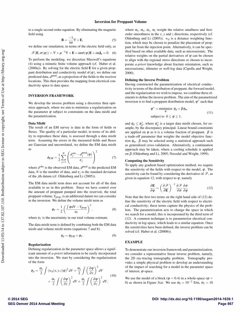
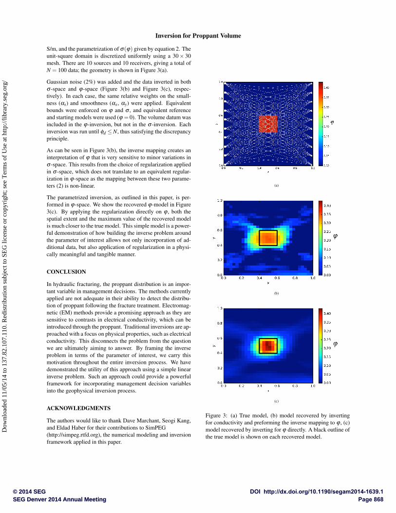
S/m, and the parametrization of s(j) given by equation 2. Theunit-square domain is discretized uniformly using a 30⇥ 30mesh. There are 10 sources and 10 receivers, giving a total ofN = 100 data; the geometry is shown in Figure 3(a).

Gaussian noise (2%) was added and the data inverted in boths -space and j-space (Figure 3(b) and Figure 3(c), respec-tively). In each case, the same relative weights on the small-ness (as) and smoothness (ax, ay) were applied. Equivalentbounds were enforced on j and s , and equivalent referenceand starting models were used (j = 0). The volume datum wasincluded in the j-inversion, but not in the s -inversion. Eachinversion was run until fd N, thus satisfying the discrepancyprinciple.

As can be seen in Figure 3(b), the inverse mapping creates aninterpretation of j that is very sensitive to minor variations ins -space. This results from the choice of regularization appliedin s -space, which does not translate to an equivalent regular-ization in j-space as the mapping between these two parame-ters (2) is non-linear.

The parametrized inversion, as outlined in this paper, is per-formed in j-space. We show the recovered j-model in Figure3(c). By applying the regularization directly on j , both thespatial extent and the maximum value of the recovered modelis much closer to the true model. This simple model is a power-ful demonstration of how building the inverse problem aroundthe parameter of interest allows not only incorporation of ad-ditional data, but also application of regularization in a physi-cally meaningful and tangible manner.

CONCLUSION

In hydraulic fracturing, the proppant distribution is an impor-tant variable in management decisions. The methods currentlyapplied are not adequate in their ability to detect the distribu-tion of proppant following the fracture treatment. Electromag-netic (EM) methods provide a promising approach as they aresensitive to contrasts in electrical conductivity, which can beintroduced through the proppant. Traditional inversions are ap-proached with a focus on physical properties, such as electricalconductivity. This disconnects the problem from the questionwe are ultimately aiming to answer. By framing the inverseproblem in terms of the parameter of interest, we carry thismotivation throughout the entire inversion process. We havedemonstrated the utility of this approach using a simple linearinverse problem. Such an approach could provide a powerfulframework for incorporating management decision variablesinto the geophysical inversion process.

ACKNOWLEDGMENTS

The authors would like to thank Dave Marchant, Seogi Kang,and Eldad Haber for their contributions to SimPEG(http://simpeg.rtfd.org), the numerical modeling and inversionframework applied in this paper.

(a)

(b)

(c)

Figure 3: (a) True model, (b) model recovered by invertingfor conductivity and preforming the inverse mapping to j , (c)model recovered by inverting for j directly. A black outline ofthe true model is shown on each recovered model.

Page 868SEG Denver 2014 Annual MeetingDOI http://dx.doi.org/10.1190/segam2014-1639.1© 2014 SEG

Dow

nloa

ded

11/0

5/14

to 1

37.8

2.10

7.11

0. R

edis

trib

utio

n su

bjec

t to

SEG

lice

nse

or c

opyr

ight

; see

Ter

ms

of U

se a

t http

://lib

rary

.seg

.org

/

http://dx.doi.org/10.1190/segam2014-1639.1 EDITED REFERENCES Note: This reference list is a copy-edited version of the reference list submitted by the author. Reference lists for the 2014 SEG Technical Program Expanded Abstracts have been copy edited so that references provided with the online metadata for each paper will achieve a high degree of linking to cited sources that appear on the Web. REFERENCES

Berryman, J. G., and G. M. Hoversten, 2013, Modelling electrical conductivity for earth media with macroscopic fluid-filled fractures: Geophysical Prospecting, 61, no. 2, 471–493, http://dx.doi.org/10.1111/j.1365-2478.2012.01135.x.

Bruggeman, D. A. G., 1935, Berechnung verschiedener physikalischer Konstanten von heterogenen Substanzen. I. Dielektrizitätskonstanten und Leitfähigkeiten der Mischkörper aus isotropen Substanzen (The calculation of various physical constants of heterogeneous substances. I. The dielectric constants and conductivities of mixtures composed of isotropic substances): Annalen der Physik, 416, no. 7, 636–664 (in German), http://dx.doi.org/10.1002/andp.19354160705.

Cipolla , C. L., and C. A. Wright, 2000, Diagnostic techniques to understand hydraulic fracturing: What? Why? and How?: Gas Technology Symposium, Society of Petroleum Engineers/Canadian Energy Research Institute, Proceedings, SPE-59735-MS.

Haber, E., U. M. Ascher, D. A. Aruliah, and D. W. Oldenburg, 2000a, Fast simulation of 3D electromagnetic problems using potentials : Journal of Computational Physics, 163, no. 1, 150–171, http://dx.doi.org/10.1006/jcph.2000.6545.

Haber, E., U. M. Ascher, and D. W. Oldenburg, 2000b, On optimization techniques for solving nonlinear inverse problems: Inverse Problems, 16, no. 5, 1263–1280, http://dx.doi.org/10.1088/0266-5611/16/5/309.

Heagy, L. J., and D. W. Oldenburg, 2013, Investigating the potential of using conductive or permeable proppant particles for hydraulic fracture characterization: 83rd Annual International Meeting, SEG, Expanded Abstracts, 576–580.

King, G. E., 2010, Thirty years of gas shale fracturing: What have we learned?: Annual Technical Conference and Exhibition, Society of Petroleum Engineers, Proceedings, SPE 133456.

Montgomery, C. T., and M. B. Smith, 2010, Hydraulic fracturing: History of an enduring technology: Journal of Petroleum Technology, 2010, no. 12, 26–32.

Nocedal, J., and S. J. Wright, 1999, Numerical optimization, 2nd ed.: Springer.

Oldenburg, D., and Y. Li, 2005, Inversion for applied geophysics: A tutorial, in D. K. Butler, ed., Near-surface geophysics: SEG, 89–150.

Shafiro, B., and M. Kachanov, 2000, Anisotropic effective conductivity of materials with nonrandomly oriented inclusions of diverse ellipsoidal shapes: Journal of Applied Physics, 87, no. 12, 8561–8569, http://dx.doi.org/10.1063/1.373579.

Torquato, S. , 2002, Random heterogeneous materials: Microstructure and macroscopic properties: Springer.

Ward, S. H., and W. Hohmann, 1988, Electromagnetic theory for geophysical applications, in M. N. Nabighian, ed., Electromagnetic methods in applied geophysics: SEG, 130–311.

Page 869SEG Denver 2014 Annual MeetingDOI http://dx.doi.org/10.1190/segam2014-1639.1© 2014 SEG

Dow

nloa

ded

11/0

5/14

to 1

37.8

2.10

7.11

0. R

edis

trib

utio

n su

bjec

t to

SEG

lice

nse

or c

opyr

ight

; see

Ter

ms

of U

se a

t http

://lib

rary

.seg

.org

/