PARAMETRIC STUDY OF FACTORS AFFECTING CAPILLARY …

The Pennsylvania State University

The Graduate School

Department of Energy and Mineral Engineering

PARAMETRIC STUDY OF FACTORS AFFECTING

CAPILLARY IMBIBITION IN FRACTURED POROUS MEDIA

A Dissertation in

Petroleum and Mineral Engineering

by

Chung-Hao Lee

© 2011 Chung-Hao Lee

Submitted in Partial Fulfillment

of the Requirements

for the Degree of

Doctor of Philosophy

May 2011

ii

The dissertation of Chung-Hao Lee was reviewed and approved* by the following:

Zuleima T. Karpyn Assistant Professor of Petroleum and Natural Gas Engineering Quentin E. and Louise L. Wood Faculty Fellow in Petroleum and Natural Gas Engineering Dissertation Advisor Chair of Committee Yaw D. Yeboah Professor and Department Head of Energy and Mineral Engineering Turgay Ertekin Professor of Petroleum and Natural Gas Engineering George E. Trimble Chair in Earth and Mineral Sciences Derek Elsworth Professor of Energy and Geo-Environmental Engineering John Yilin Wang Assistant Professor of Petroleum and Natural Gas Engineering Kamini Singha Assistant Professor of Geosciences

*Signatures are on file in the Graduate School

iii

ABSTRACT

Capillarity, gravity and viscous forces control the fluids migration in geologic

formations. However, experimental working addressing the simultaneous action of these

driving forces as well as the impact of injection flow rate in fractured porous media is

limited. Understanding how these variables affect fracture-matrix transfer mechanisms

and invasion front evolution in fractured rocks are of crucial importance to modeling and

prediction of multiphase ground flow. This study addresses the simultaneous influence of

fracture orientation, rock and fluid properties, and flowing conditions on multiphase flow

in fractured permeable media at laboratory scale. Displacement of a non-wetting phase

(gas or liquid) by capillary imbibition was monitored using X-ray computed tomography

(CT). Results were then mimicked using an automated history matching approach to

obtain representative relative permeability and capillary pressure curves to further

investigate the impact of matrix homogeneity/heterogeneity and boundary shape on the

response of the imbibition front. Sensitive analyses, in combination with direct

experimental observation, allowed us to explore relative importance of relative

permeability and capillary pressure curves to saturation distribution and imbibing font

evolution.

Experimental observations combined with simulation results indicated the impact of

fracture orientation on imbibition front evolution was minimal for the time- and length-

scales considered in this investigation. While different injection rates and fluid types

showed significant differences in the shape of the imbibing front, breakthrough time, and

saturation profiles. The speed and shape of imbibing front progressions were found to be

sensitive to matrix water relative permeability, capillary pressure contrast between matrix

and fracture, and degree of rock heterogeneity. Results from this work also demonstrated

conditions that favor co-current, counter-current, and the coexistence of both

displacement mechanisms during imbibition. Co-current flow dominates in the case of

water displacing air, while counter-current flow dominates in the case of water displacing

iv

kerosene. The balance of capillarity and relative permeabilities has a significant impact of

the shape on the invasion front, resulting in periods of co-current and counter-current

imbibition. This work presents direct evidence of spontaneous migration of wetting fluids

into a rock matrix embedding a fracture. These observations and conclusions are not

limited by the geometry of the system and have important implication for water flooding

of naturally fractured reservoir and leak-off retention and migration after hydraulic

fracture treatments.

v

TABLE OF CONTENTS

Pages

LIST OF FIGURES .......................................................................................................... vii

LIST OF TABLES ............................................................................................................. xi

ACKNOWLEDGEMENTS .............................................................................................. xii

Chapter 1 Introduction ....................................................................................................... 1

Chapter 2 Experimental Investigation of Rate Effects ...................................................... 3

2.1 Literature Review ..................................................................................................... 3

2.2 Experiment Design ................................................................................................... 5

2.2.1 Sample Holder ............................................................................................... 6

2.2.2 X-ray CT scanner ........................................................................................... 8

2.2.3 Fluid Circulation System ............................................................................... 9

2.3 Experimental Procedure ......................................................................................... 11

2.4 Determination of Porosity and Fluid Saturation .................................................... 12

2.5 Results and Discussion ........................................................................................... 12

Chapter 3 Impact of Viscosity Ratio and Fracture Orientation ....................................... 18

3.1 Literature Review ................................................................................................... 18

3.2 Experimental Design .............................................................................................. 20

3.3 Experiment Procedure and Determination of Porosity and Fluid Saturation ......... 22

3.4 Results and Discussions ......................................................................................... 23

3.4.1 Impact of Viscosity Ratio ............................................................................ 23

3.4.2 Impact of Fracture Orientation ..................................................................... 29

Chapter 4 Numerical Analysis of Imbibition Front Evolution and History Matching .... 35

4.1 Literature Review ................................................................................................... 35

4.2 Automated History Matching Approach ................................................................ 38

4.3 Sensitivity Analysis ................................................................................................ 42

vi

4.4 History Matching Results and Validation .............................................................. 49

4.5 Predictive Cases ..................................................................................................... 59

Chapter 5 Conclusions ..................................................................................................... 64

References ......................................................................................................................... 66

Appendix A Derivative of Porosity and Fluid saturations from CT Scans.................. 70

Appendix B Matlab Code for Automated History Matching ...................................... 75

vii

LIST OF FIGURES

Pages

Figure 2-1: Schematic drawing of experimental design. .................................................... 5

Figure 2-2: Schematic drawing of sample holder design. ................................................... 6

Figure 2-3: Schematic drawing of flow pathway within sample holder. ............................ 7

Figure 2-4: A sample disk with fracture perpendicular to the bedding layers (left), and

Teflon core holder, Viton rubber sheets (black) and support rod (right). .................... 7

Figure 2-5: Schematic drawing of X-Ray CT Scanner. ...................................................... 8

Figure 2-6: Schematic drawing of fluid circulation system. ............................................. 10

Figure 2-7: Experimental procedure and CT scanning sequence for oil-water system. ... 11

Figure 2-8: Average water saturation as a function of time, showing the effect of injection

rate. ............................................................................................................................ 14

Figure 2-9: Time progression of water saturation maps corresponding to 40mL/hr (top)

and 4mL/hr (bottom) brine injection rate, kerosene-brine experiment. ..................... 15

Figure 2-10: Vertical saturation profiles perpendicular to the fracture and averaged over

the central 6 mm of the sample, Kerosene-brine experiment, q=40mL/hr (left) and

q=4mL/hr (right). ....................................................................................................... 17

Figure 3-1: Five different fracture configurations. ........................................................... 20

Figure 3-2: Experimental procedure and CT scanning sequence for air-water system. ... 22

Figure 3-3: Average water saturation as a function of time and PVI for different fluid

pairs. ........................................................................................................................... 24

Figure 3-4: Sequence of water saturation maps obtained from CT scanning at 4mL/hr

water injection rate for different fluid pairs. .............................................................. 27

viii

Figure 3-5: Vertical Saturation profiles perpendicular to the fracture and averaged over

the central 6 mm of the sample, for different ............................................................ 28

Figure 3-6: Average water saturation as a function of pore volume injected (PVI) for

different fracture orientations. ................................................................................... 30

Figure 3-7: Sequence of water saturation maps obtained from CT scanning at 4mL/hr

water injection rate for different fracture orientations. .............................................. 31

Figure 3-8: Saturation maps showing air (circular shadow) trapped in the fracture zone as

water injected time equals to 61 minutes. .................................................................. 32

Figure 3-9: Saturation maps showing air snap-off in the fracture. ................................... 33

Figure 3-10: Vertical Saturation profiles perpendicular to the fracture and averaged over

the central 6 mm of the sample, in the case of vertical fracture flowing down and

vertical fracture flowing up. ...................................................................................... 34

Figure 4-1: Schematic diagram of history matching approach (Basbug and Karpyn

(2008)). ...................................................................................................................... 39

Figure 4-2: Matrix and fracture relative permeability curves (left) and capillary pressure

curves (right) used in sensitivity analysis case A. ..................................................... 42

Figure 4-3: Matrix relative permeability curves (left) and capillary pressure curves (right)

for sensitivity analysis cases A, B. ............................................................................ 43


for sensitivity analysis cases A, C. ............................................................................ 44


for sensitivity analysis cases A, D. ............................................................................ 44

Figure 4-6: Average water saturation as a function of time for sensitivity cases A, B, C

and D. ......................................................................................................................... 45

Figure 4-7: Sequence of water saturation maps at 4mL/hr water injection rate for

sensitivity cases A, B, C and D.................................................................................. 46

ix


the central 6 mm of the simulation model, q=4mL/hr at time=80 minutes for

sensitivity analysis cases A, B, C and D. ................................................................... 48

Figure 4-9: Matrix and fracture relative permeability curves obtained from history

matching method. ...................................................................................................... 50

Figure 4-10: Capillary pressure curves on both matrix and fracture obtained from history

matching method. ...................................................................................................... 50

Figure 4-11: Comparison of experimental and history matched relative permeability

curves. ........................................................................................................................ 51

Figure 4-12: Comparison of experimental and modeled average water saturation as a

function of time at 4mL/hr water injection rate. ........................................................ 52

Figure 4-13: Comparison of experimental and modeled water saturation maps at 4 mL/hr

water injection rate. ................................................................................................... 53

Figure 4-14: Comparison of experimental and modeled vertical saturation profiles

perpendicular to the fracture and averaged over the central 6 mm of the sample,

q=4mL/hr. .................................................................................................................. 54

Figure 4-15: Comparison of experimental and predicted average water saturation as a

function of time at 40mL/hr water injection rate. ...................................................... 56

Figure 4-16: Comparison of experimental and predicted water saturation maps at 40

mL/hr water injection rate. ........................................................................................ 57

Figure 4-17: Comparison of experimental and predicted vertical saturation profiles


q=40mL/hr. ................................................................................................................ 58

Figure 4-18: Matrix porosity (left) and permeability (right) histograms for cases A and F.

................................................................................................................................... 60

x

Figure 4-19: Average water saturation as a function of time at 4mL/hr water injection rate

for cases A, E, F and G. ............................................................................................. 61

Figure 4-20: Predicted sequence of water saturation maps at 4mL/hr water injection rate

for cases A, E, F and G. ............................................................................................. 63

xi

LIST OF TABLES

Pages

Table 2-1: Physical properties of fluids. ........................................................................... 10

Table 3-1: Physical properties of fluids. ........................................................................... 21

Table 3-2: Capillary numbers and Bond numbers correspond to three fluid pairs. .......... 22

Table 4-1: Rock properties assigned to fracture and matrix in simulation model. ........... 41

Table 4-2: Lists of investigated parameters in sensitivity analysis cases. ........................ 42

Table 4-3: Standard deviation of porosity and permeability for cases A, E, F and G. ..... 59

xii

ACKNOWLEDGEMENTS

I want to express my deep appreciation and unlimited thanks to my family, especially my

wife, Annie and my daughters, Evelyn and Melody for their support, patience,

understanding and sacrifice. This study would not have been accomplished without them.

I would like to express my gratitude and appreciation to the thesis advisor, Dr. Zuleima

T. Karpyn for her continues support, guidance and encouragement. She has been very

helpful, encouraging and patient during challenging periods both in my research and my

personal life. I also would like to thank the committee members, Dr. Turgay Ertekin, Dr.

Derek Elsworth, Dr. John Yilin Wang and Dr. Kamini Singha for their guidance and

positive criticism.

Special thanks go to Dr. Phillip Halleck and friends who had contributed to my graduate

study and my life experience at Penn State, and thanks Center for Quantitative Imaging

(CQI) laboratory, Energy Institute, PSU and National Science Foundation (NSF),

GeoEnvironmental Engineering and Geohazard Mitigation to support this study.

Chapter 1

Introduction

Fractures serve as primary conduits having great impact on the migration of injected fluid

into fractured permeable media. This research study is a multi-variable analysis of

fracture-matrix flow including the effects of injection flow rate, fluid type, fracture

orientation and flow direction. In the first section of this study (see Chapter 2), we

analyze the impact of two different injection rates on the capillary dominated

displacement of oil by water in fractured rock samples, using x-ray computed

tomography. A laboratory flow apparatus was designed specifically for this set of

experiment, in which saturation maps are monitored as a function of time for two

injection flow rates. X-ray computed tomography (CT) was used to record these

saturation maps as a function of time. Continuous CT scanning allowed us to track

capillary imbibition into a fractured Berea sandstone sample originally saturated with

kerosene.

Experiments were later extended to cover different fluid types and five different fracture

configurations with flow directions (see Chapter 3). This experimental investigation

addresses the influence of viscosity ratio and fracture orientation on the progression of an

imbibition front in fractured permeable media at laboratory scale. Three different fluid

pairs including air-brine, kerosene-brine and a viscous oil-brine, and five different

fracture configurations were investigated to address the influence of viscosity ratio and

fracture orientation on oil recovery and saturation maps. Experimental results of two-

phase (kerosene-brine) floods are then mimicked using an automated history matching

approach to obtain representative matrix and fracture relative permeability and capillary

pressure curves (see Chapter 4). These curves were then used to predict imbibition front

evolution under different flow conditions, which result in excellent agreement with

2

experimental observations. Sensitivity analyses and predictive simulation tests were

provided to further investigate the effects of transport properties and shapes of boundary

on oil displacement and imbibition front evolution. Results from this investigation

provide a comprehensive set of data for the validation of numerical models and

strengthen fundamental understanding of multiphase flow in fractured rocks.

Chapter 2

Experimental Investigation of Rate Effects

Understanding how injection flow rate affects fracture-matrix transfer mechanisms and

invasion front evolution in fractured reservoirs are of crucial importance to modeling and

prediction of multiphase ground flow. However, experimental work addressing the

impact of injection flow rate in fractured core samples is limited. In this chapter, we

monitor and analyze transfer mechanisms in fractured rock samples using medical X-ray

computed tomography. The impact of different injection rates on the resulting fluid

recovery and saturation maps is evaluated through visual and quantitative analyses.

Results from this work help visualize the impact of injection flow rate on the dynamics of

fracture-matrix transport and, at the same time, provide detailed quantitative information

for the validation of representative numerical models of fractured permeable reservoirs.

2.1 Literature Review

Fluid displacement in fractured media is of interest for many environmental and

engineering processes. Examples include CO2 geological sequestration, nuclear waste

disposal, geothermal power generation, and enhanced oil recovery in natural fracture

reservoir (Berkowitz (2002); Committee on Fracture Characterization and Fluid Flow

(1996)). The presence of fractures not only provide preferential pathways for fluid

migration, but also gives rise to a range of complex flow phenomena. Crandall et al.

(2010) conducted a series of simulations for flows in fractured permeable rocks, and

observed more than 5% increase in the volumetric flow rate within high permeability-

fractured porous media. Karpyn et al. (2009) found that bedding planes adjacent to

fracture zones with higher aperture tend to have higher porosity, and higher permeability,

thus affecting the overall hydraulic conductivity of the system. This higher hydraulic

conductivity leads to higher flow rate in the fracture zone and makes injected fluids easily

4

breakthrough and low efficiency displacement in the porous matrix. Alajmi and Grader

(2000) used x-ray CT to study two-phase flow displacements in layered Berea samples

with fracture tips. The results showed the presence of the fracture significantly delayed

the oil recovery. In addition, different flow behaviors, co-current and counter-current

imbibition were observed at three different regions in the sample, the fracture region, the

non-fractured region, and the fracture tip. Rangel-German and Kovscek (2002) used x-

ray CT to study capillary imbibition of air and oil displacement by water from rock

samples. They identified two different fracture flow regimes, co-current and counter-

current imbibition. Counter-current imbibition is occurring when the fractures refills with

water at a faster rate than it can be transferred through the fracture-matrix interface, while

co-current shows when relatively slow flow through fractures.

Different flow regimes were observed at different injection flow rate. Melean et al.

(2003) conducted a series of imbibition experiments in porous medium at different

injection rates by using CT scan measurements. The results showed the water front

spread smoothly and increased evenly at low rates, while the water front spread rapidly

and inclined to the outlet at high rate cases. Babadagli (1994) found that as the injection

rate is increased, fracture pattern becomes an important parameter controlling the

saturation distribution in the rock matrix. As the rate is lowered, however, the system

begins to behave like a homogeneous system showing a frontal displacement regardless

of the fracture configuration. Similar observation can be obtained from Babadagli (2000).

Although these, and other studies (Prodanovic et al. (2008), Hoteit and Firoozabadi

(2008), Donato et al. (2007), and Rangel-German et al. (2006)) have contributed to

current understanding of multiphase flow in fractured systems, there is still limited

understanding of the relative impact of injection rate affecting two-phase displacement

mechanisms in fractured rocks. Analyzing how injection rate affects fracture-matrix flow,

especially under capillary dominated conditions, remains largely unexplored and it is the

main goal of this section.

5

2.2 Experiment Design

The purpose of this design was to create a two-dimensional flow system within a sample

holder, to allow complete sample monitoring with a single-slice CT scanning as shown in

Figure 2-1. By making the sample a thin disk, we eliminate one flow direction, the one

orthogonal to the disk. Therefore, a single slice is sufficient to capture the entire fracture

and the surrounding rock matrix, thereby allowing us to keep track of saturation changes

at small time intervals. The rock sample used in this study was Berea Sandstone. Each

sample disk has a diameter of 102 mm and thickness of 10 mm. A single tensile fracture

was created artificially on each disk. All fractures are aligned with the centre of the

sample and perpendicular to the bedding layers. Fracture apertures are around 0.5mm.

Pore volume of the matrix and fracture are 18.51mL and 0.51mL, respectively. The

experimental apparatus includes three major portions: sample holder, fluid supply system

and X-ray CT scanner.

Figure 2-1: Schematic drawing of experimental design.

360o

Supporting

rod

Scanned section

6

2.2.1 Sample Holder

A cake-shaped sample holder was fabricated according to the diagram shown in Figure 2-

2 and Figure 2-3. After assembling pieces A, B and inserting piece C, a trapped volume is

obtained with a diameter of 104 mm and a thickness of 10 mm. This sample holder is

made of Teflon to avoid chemical reaction with fluids, and only Teflon and the rock

sample are intercepted by the scanning plane. Viton rubber sheets are used to seal the gap

between the sample and the walls of the holder, thus blocking potential pathways around

the sample and allowing fluid flow through the fracture alone. The supporting rod, also

shown in the top-right insert in Figure 2-1, can rotate in 45 degree increments, and it is

attached in such a way that the cell can rotate on its horizontal axis. Although the core

holder is designed to allow different fracture inclinations and flow directions with this

rotation system, this section focuses on experiments using a horizontal fracture. A similar

rotation system was used in a core holder designed for gravity segregation experiments

by Karpyn et al. (2006). Figure 2-4 (left) shows a sample disk with fracture

perpendicular to the bedding layers and Figure 2-4 (right) shows a photograph of all the

pieces forming the core holder.

Figure 2-2: Schematic drawing of sample holder design.

h=10 mm

Diameter =102 mm

SampleA

B

C

7

Figure 2-3: Schematic drawing of flow pathway within sample holder.

Figure 2-4: A sample disk with fracture perpendicular to the bedding layers (left), and

Teflon core holder, Viton rubber sheets (black) and support rod (right).

Sample

Inlet

Flow out

Flow out

Outlet

OutletInlet

Sample

Flow out

fracture

8

2.2.2 X-ray CT scanner

Fluid saturation distributions are computed using X-ray computed tomography (CT)

scanning. X-Ray CT is a non-destructive imaging technique that uses X-rays and

mathematical reconstruction algorithms to view the internal properties of an object

(Vinegar and Wellington (1987)). It is also used to quantify rock heterogeneities,

determine lithologies and porosities, and monitor fluid saturations during flow processes.

A medical HD350 scanner with a detection limit of 25 microns was used in this study.

The CT system consists of an ionized X-Ray source, a detector, a translation system, and

a computer system that controls motions and data acquisition. Each CT image produces a

matrix of 512 by 512 pixels covering the entire sample. The voxel size selected to this

work was 5.00×0.205×0.205 mm. Figure 2-5 shows the schematic drawing of medical

CT scanner used in this study, which locates in the Center for Quantitative X-Ray

Imaging (CQI) at Penn State University.

Figure 2-5: Schematic drawing of X-Ray CT Scanner.

X-Ray Detector

(Stationary)

X-Ray tube

(Rotating)

0.2mm

0.2mm 5mm

Voxel size

512×512 pixels

covering the entire

sample

512 pixels

51

2p

ixel

s

9

2.2.3 Fluid Circulation System

The fluids used in the present experiments are distilled water and kerosene. Distilled

water was tagged with 15% by weight of sodium iodide (NaI) to increase its CT

registration and provide a high contrast between the two phases. The viscosity of tagged

water is approximately 1.80 cP (centipoise) and that for kerosene is 4.06cP. The physical

properties of these fluids are shown in Table 2-1. Before commencing the experiment,

two immiscible fluids, oil and water phases, were thoroughly mixed with each other and

allowed to separate under gravity action. This procedure minimizes in-situ changes in

saturation due to mutual solubility.

A schematic representation of this system is presented in Figure 2-6. A vacuum pump

enables the sample holder reach 250 microns vacuum condition. This vacuum state is

used to pre-saturate the sample with oil phases. A syringe pump (LC-5000) delivers

tagged water (brine) into the sample through the fracture. To guarantee a predominantly

capillary-driven displacement, injection flow rates are low, in the order of 40mL/hr and

4mL/hr, which correspond to capillary numbers in the order of 4.8×10-4

and 4.8×10-5

,

respectively. The capillary number represents the relative control of viscous force over

capillary force. For capillary numbers below 10-5

, flow in porous media is considered to

be dominated by capillary forces (Ding and Kantzas (2007)). The equation for calculating

the capillary number is

vN ca

...........................................................................................................[2-1]

where μ is the viscosity of the liquid, v is a characteristic velocity and γ is the surface or

interfacial tension between the two fluid phases.

10

Figure 2-6: Schematic drawing of fluid circulation system.

Table 2-1: Physical properties of fluids.

Phases Fluid composition Viscosity at

25.7ºC (cP)

Specific gravity at

25.7ºC

Water Tagged water

(15% NaI by weight) 1.0 1.0

Oil Kerosene 2.9 0.79

X-Ray

Source

X-Ray

Detector

P

Drain

V

Non-wetting

phase fluid

Brine

Quizix pump

(SP-5200 )

Vacuum pump

Sample

Holder

11

2.3 Experimental Procedure

A schematic representation of the experimental procedure is presented in Figure 2-7. The

dry fractured sample was mounted and vacuumed in the sample holder and scanned to

observe its heterogeneity and its layered structure (stage 1 in Figure 2-7). In stage 2, the

sample was pre-saturated with oil (non-wetting phase) and scanned. The image difference

between these two stages is used for porosity calculations. In stages 3 and 4, the sample

was flooded by injecting water. Fluid saturations were continuously monitored by

scanning at specific time intervals until residual oil saturation was reached. At the same

time, oil recovery is recorded as a function of time at the outlet.

Figure 2-7: Experimental procedure and CT scanning sequence for oil-water system.

1. Vacuum sample

and scan

3. Begin water

injection

4. End of water

injection

2. Saturate sample

and scan

Scan slice filled

with non-wetting

phase. This will be a

reference state

Scan dry slice for

fracture

identification and

rock heterogeneities

Start continuous

scanning of slice

during water

injection

Continue Scanning

during water

injection

12

2.4 Determination of Porosity and Fluid Saturation

The average sample porosity (avg ) is 23.27% obtained from the volume of oil used in

saturating the sample and the bulk volume of the sample. Pixel porosities (pixel ) were

obtained from Equation [2-2] using X-ray CT registrations from the vacuum condition in

stage 1( vacuumCT ) and the oil saturated condition in stage 2 ( satCT ) as shown in Figure

2-7.

avg

avgvacuumsat

vacuumsatpixel

CTCT

CTCT

……………………………………………....…......[2-2]

In situ saturations were also determined using data from the CT scanner. Pixel water

saturations (pixelwS ,

) were obtained from Equation [2-3], where pixel is the pixel porosity

from Equation [2-2], avgwS ,

is the average saturation of water in the sample obtained from

the linear correlation between 100% water saturated ( avgwCT , ) and 100% oil saturated

sample ( avgsatCT , ).

avgw

pixel

avg

avgfsat

fsat

pixelw SCTCT

CTCTS ,,

….……………..............………….…………….…….….... [2-3]

avgsatavgw

avgsatavgf

avgwCTCT

CTCTS

,,

,,

,

……..………..................................……………………….…….….[2-4]

2.5 Results and Discussion

In this section, we compare two different injection flow rates using the same fluid type,

kerosene and brine. Average saturation changes as a function of time and pore volume

injected are presented in Figure 2-8. These saturations were averaged over the entire

sample, including fracture and rock matrix. In Figure 2-8 top, water breakthrough for the

low-rate curve in red is delayed 10 min with respect to the high-rate blue curve. In

addition, the high-rate curve (q=40mL/hr) reaches higher water saturation, and thus

higher oil recovery, sooner than the low-rate case, but it requires more pore volume

13

injected to reach that saturation level, as seen in Figure 2-8 bottom. After approximately

300 minutes of water injection, oil recovery becomes negligible in both cases, when

water saturation reaches 0.56. Under this final saturation conditions, both oil and water

are still mobile inside the rock sample, but the increments in water saturation are too

small to be appreciated in the lapse of a few days.

Figure 2-9 are time progressions of water saturation (Sw) maps corresponding to high

and low water injection rate. Dark blue represents regions saturated with kerosene

(Sw=0.0), red represents regions saturated with water (Sw=1.0), and intermediate colors

represent the co-existence of kerosene and water in the pore space. For the high-rate case

(Figure 2-9 top) we see a sharp increase in water saturation in the neighborhood of the

fracture, and a maximum in the fracture itself and the outlet (right end of the fracture).

Under these flowing conditions, the fractures refills with water at a faster rate than it can

be transferred through the fracture-matrix interface, confirming similar experimental

observations found in the literature (Rangel-German and Kovscek (2006)).

Simultaneously, counter-current imbibition is occurring in the water invaded zone as oil

is expelled from the matrix into the fracture. As time progresses, the imbibition front

moves away from the fracture, and water accumulation becomes evident around the

outlet end of the fracture (right side) in red, supporting the fact that the rate of capillary

dispersion through the matrix is low compared to the rate of injection. The rate of

injection is also responsible for the shape of the imbibing front, which is farther away

from the fracture inlet than the outlet. These mechanistic observations are less

pronounced when the rate of injection is reducing.

Figure 2-9 bottom shows an analogous progression of water saturation maps obtained at

4mL/hr of water injection. The contrast in saturation ahead and behind the water front is

not as sharp as that in Figure 2-9 top. This is evident in a smoother color transition,

passing from dark to light blue, to green, and finally yellow and red.

14

Figure 2-8: Average water saturation as a function of time, showing the effect of injection rate.

0

0.1

0.2

0.3

0.4

0.5

0.6

0.7

0.8

0.9

1

0 2 4 6 8 10 12 14 16 18 20 22 24 26 28 30 32 34 36 38 40 42 44 46 48 50 52

Av

era

ge

wa

ter

satu

rati

on

Pore volume injected

q=40mL/hr, kerosene-brine


0

0.1

0.2

0.3

0.4

0.5

0.6

0.7

0.8

0.9

1

0 200 400 600 800 1000 1200 1400 1600 1800 2000 2200 2400 2600 2800 3000 3200 3400 3600 3800 4000 4200 4400 4600

Av

era

ge

wa

ter

satu

rati

on

Time, min



15

Figure 2-9: Time progression of water saturation maps corresponding to 40mL/hr (top) and 4mL/hr (bottom) brine injection rate,

kerosene-brine experiment.

0.0

0.2

0.4

0.6

0.8

1.0

0.9

0.7

0.5

0.3

0.1

Sw

Q=4 mL/hr

10min 30min 50min 80min 110min 170min 230min 1430min

Q=40 mL/hr


16

In addition, for the same pore volume injected, that is 0.7 PVI at 20 min high-rate

(40mL/hr) and 170 min low-rate (4mL/hr), we observe a much larger imbibed region in

the low-rate case, implying low injection rate allows a more effective spreading of water

for the same volume injected. At the late time (t=1440), water collects around the

fracture's outlet end. This is depicted by the red cone shape observed at the right side of

the sample.

Further quantitative examination of saturation changes obtained from CT scanning is

presented in Figure 2-10. These vertical saturation profiles averaged over the central 6

mm of each CT slice for the two flow rates under study. These profiles capture saturation

changes with time in the direction perpendicular to the fracture. For both experiments,

continuous high water saturation is observed in the center of the sample, where the

fracture is located. The most salient differences between these two groups of vertical

profiles are: (1) the speed at which the water front moves away from the fracture, which

was also evident in the saturation maps, presented in Figure 2-9; and (2) the change in

saturation as we move away from the fracture. Figure 2-10 right shows a gradual

saturation change at the front, while there is a drastic drop in saturation across the water

front in Figure 2-10 left. Furthermore, water saturations remain in the 0.50-to-0.55 range

within the imbibed zone, which suggests that both fluid phases are under a dynamic

equilibrium at that saturation. This is consistent with the knowledge that counter-current

flow is the prevalent flow mechanism in the imbibed zone. As the water front progresses,

the resident oil is displaced towards the fracture, in a counter-current manner, and

replenished by the oil that is sitting ahead of the front, thus maintaining a dynamic

equilibrium and a constant saturation in the imbibed zone.

17

Figure 2-10: Vertical saturation profiles perpendicular to the fracture and averaged over the central 6 mm of the sample, Kerosene-

brine experiment, q=40mL/hr (left) and q=4mL/hr (right).

-50

-40

-30

-20

-10

0

10

20

30

40

50

0 0.2 0.4 0.6 0.8 1

Dis

tan

ce fro

m f

ra

ctu

re (

mm

)

Sw

T=10min

T=20min

T=60min

T=120min

T=180min

T=1440min

-50

-40

-30

-20

-10

0

10

20

30

40

50

0 0.2 0.4 0.6 0.8 1D

ista

nce fro

m f

ra

ctu

re (

mm

)

Sw

T=10min

T=20min

T=60min

T=120min

T=180min

T=1440min

Injection Rate=40mL/hr Injection Rate=4mL/hr

Area of

interest

6 mm

Area of

interest

6 mm

Chapter 3

Impact of Viscosity Ratio and Fracture Orientation

The objective of this section is to investigate the effects of viscosity ratio and fracture

orientation on oil recovery and water front evolution using medical X-Ray computed

tomography (CT). First, we compare three different fluid pairs with different viscosity

ratio in horizontal fractured rock samples. These experiments were then extended to

include five different fracture configurations in the case of water displacing air to

evaluate the impact of fracture orientations. A detailed delineation of the impact of

viscosity ratio as well as fracture orientation on the dynamics of fracture-matrix transport

is presented and provides reference background to qualify the migration and trapping of

leak-off fracturing fluids in hydraulic fracture under shut-in conditions.


In general, capillarity, gravity and viscous force are three major driving forces control

fluids migration in geological formations. Numerous studies had demonstrated the

importance of these forces whether from experiments (Lefebvre du prey (1978), Ovdat

and Berkowitz (2006)) or simulation models (Ajose and Mohanty (2003)).

Ide et al. (2007) used simulation model to investigate the impacts of gravity and viscous

forces on capillary trapping of CO2. Results showed that effects of capillary pressure and

aquifer inclination increased the amount of CO2 trapped. Hognesen et al. (2006)

conducted a series of experiments to identify capillary and gravity dominated flow

regimes and concluded that the impact of gravity decreased as the height of the core

decreased.

The simultaneous action between capillarity, gravity and viscous forces becomes more

complex in fractured geological formation (Berkowitz (2002)).When a wetting fluid

19

flows through a fracture, capillarity may drives the wetting fluid from the fracture into

the matrix, while viscous force propels the fluid to flow through the fracture with less

resistance. Rangel-German et al. (2006) stacked Boise sandstone blocks to study multi-

phase flow in a fractured system. They concluded that both capillary and viscous force

control the flow in the fracture and that capillary continuity can occur in any direction,

depending on the relative strengths of the capillary and Darcy (viscous) terms in the flow

equations. Tang and Firoozabadi (2000) conducted a series of experiments and found the

oil displacement efficiency can be significantly influenced by viscous force and gravity in

a fractured porous media. Rangel-German and Kovscek (2002) indicated the effect of

gravity on the orientation of fracture-matrix is evident through oil-water experiments.

Firoozabadi and Markeset (1992) studied gravity and capillary cross-flow in fractured

porous media, and showed that the contribution of capillary cross-flow from the side

faces of the matrix rock increased with the tilt angle. Gu and Yang (2003) used numerical

modeling to study the interfacial profile between two immiscible fluids in a reservoir

with a fracture with random orientation, and found that the equilibrium shape of the

interfacial profile depends on the ratio of gravity and capillarity.

Fracture orientation had great influence on fluid displacement under the interplay of

capillary, gravity and viscous forces. Crawford and Collins (1954) found the sweep

efficiency depends on the length and orientation of the fracture and direction of the flood.

Carnes (1966) indicated that it is essential to determine presence and orientation of a

fracture system in a reservoir since it has a significant effect on the success or failure of

water flooding. Shedid (2006) and Shedid and Zekri (2006) investigated the effect of

fracture orientation on water flooding processes. The results indicated fracture orientation

had greater influence on oil displacement, and the increase of fracture inclination angle

decreases oil displacement by water flooding. Similar experimental work were reported

by Farzaneh et al. (2010) recently with different results between the oil displacement and

the orientation angle. They conducted experimental studies and observed that the oil

displacement decreased when the fractures’ aperture, discontinuity, over-lap, and

20

distribution increased. In contrast, the oil displacement increased when the orientation

angle, discontinuity- distribution and the number of fractures increased. However,

experimental works addressing the simultaneous action of capillarity, gravity and viscous

force under the effect of different fracture orientation (where injection direction is

parallel to fracture) is limited. Understanding how these forces affects fracture-matrix

transfer mechanisms and how these mechanisms are altered by fracture orientation are of

crucial importance and are the main goals of this section.

3.2 Experimental Design

An experimental apparatus including sample holder, fluid supply system and X-Ray CT

scanner designed and constructed in the Chapter 2 was used in this study. The rock

sample used in this study was Berea Sandstone with average porosity about 22%. A

single tensile fracture was created artificially on each disk. Fractures are aligned with the

centre of the each sample and are placed perpendicular to the bedding layers. Average

fracture apertures are around 0.5mm. Pore volume of the matrix and fracture are 18.51mL

and 0.51mL respectively. Five different fracture configurations including (1) horizontal,

(2) vertical flowing up,(3) vertical flowing down,(4) diagonal flowing up, and (5)

diagonal flowing down were investigated to address the influence of fracture orientation

on the capillary imbibition in fractured permeable rock. A detailed matrix of fracture

configurations is displayed in Figure 3-1.

Figure 3-1: Five different fracture configurations.

Horizontal

fracture

Vertical fracture

flowing up

Vertical fracture

flowing down

Diagonal

fracture

flowing up

Diagonal

fracture

flowing down

0° +90° +90° -45° +45°

21

Air-brine, kerosene-brine and viscous oil-brine represent three different fluid pairs

considered in this experimental work. The viscous oil was formed by mixing 50% by

weight of n-decane and Silicone oil. Kerosene and viscous oil represent two types of oil

phase to pre-saturate the sample. Water was tagged with 15% by weight of sodium iodide

(NaI) to increase its CT registration and provide a high contrast between the two phases.

The viscosity of tagged water is approximately 1.0 cP and that for kerosene and mixture

oil are 2.9 cP and 36.32 cP, respectively. The physical properties of these fluids are

shown in Table 3-1.

Before commencing the experiment, wetting and non-wetting liquid phases, were

thoroughly mixed with each other and allowed to separate under gravity action. This

procedure minimizes in situ changes in saturation due to mutual solubility during the

displacement experiment. To guarantee a predominantly capillary-driven displacement,

injection flow rates are low, in the order of 4mL/hr, which correspond to capillary

numbers (Nca) on the order of 10-4

to 10-8

. This capillary number represents the relative

control of viscous over capillary forces. For capillary numbers below 10-5

, flow in porous

media is considered to be dominated by capillary forces (Ding and Kantzas (2007)). Bond

number (Bo) express the relative importance of gravitational to capillary forces. Table

3-2 summarizes capillary numbers and Bond numbers correspond to three different fluid

pairs.

Table 3-1: Physical properties of fluids.

Exp. Phases Fluid composition Viscosity at

25.7oC (cP)

Specific gravity at

25.7oC

Set 1 water Tagged water(15% NaI by weight) 1.0 1.0

oil Kerosene 2.9 0.79


Air Air 0.018 0.001


oil Silicone oil & Decane 50% by weight 36.32 0.83

22

Table 3-2: Capillary numbers and Bond numbers correspond to three fluid pairs.

Fluid type Nca Bo

Set 1 Kerosene 4.8 × 10-5

0.038

Set 2 Air 5.5 × 10-8

0.033

Set 3 viscous oil 2.7× 10-4

0.014

3.3 Experiment Procedure and Determination of Porosity and Fluid Saturation

Kerosene-brine and viscous oil-brine follow the same experimental procedure presented

in Figure 2-7. Air-brine system shows similar experimental procedure as presented in

Figure 3-2. The only difference between these two procedures is, in air-brine system,

since distilled water was used to saturate sample for porosity calculations in the stage 2,

additional 72 hours vacuuming and air injection was required to drain off water and

saturated with air, before starting injection as shown in stage 3.

Figure 3-2: Experimental procedure and CT scanning sequence for air-water system.

The average sample porosity (avg ) is about 22% obtained from the volume of fluid used

in saturating the sample and the bulk volume of the sample. Pixel porosities (pixel ) were

obtained from Equation [2-2] as shown in Chapter 2.4. In situ saturations were also

determined using data from the CT scanner. Pixel water saturations (pixelwS ,

) were

1. Vacuum sample

and scan

3. Drain off

distilled water

2. Saturate sample

and scan

Scan slice filled

with distilled water.

This will be a

reference state

Scan dry slice for

fracture

identification and

rock heterogeneities

Scan slice. This will

be an initial

condition

4. Begin water

injection

Start continuous

scanning of slice

during water

injection

5. End of water

injection

Continue Scanning

during water

injection

23

obtained from Equation [2-3], avgwS ,

is the average saturation of water in the sample

obtained from Equation [2-4]. Since initial water saturation exist in all air-brine

experiments, in situ saturations and average saturations need to be modified as presented

in Appendix A.2 Equation [22] and Equation [33].

3.4 Results and Discussions

3.4.1 Impact of Viscosity Ratio

In this section, we compare three different immiscible fluid pairs with different viscosity

ratios using the same injection flow rate of q=4ml/hr in horizontal fractured rock samples.

In experiment set 1, the sample was pre-saturated with kerosene; in experiment set 2, the

sample was pre-saturated with air; and in experiment set 3, the sample was pre-saturated

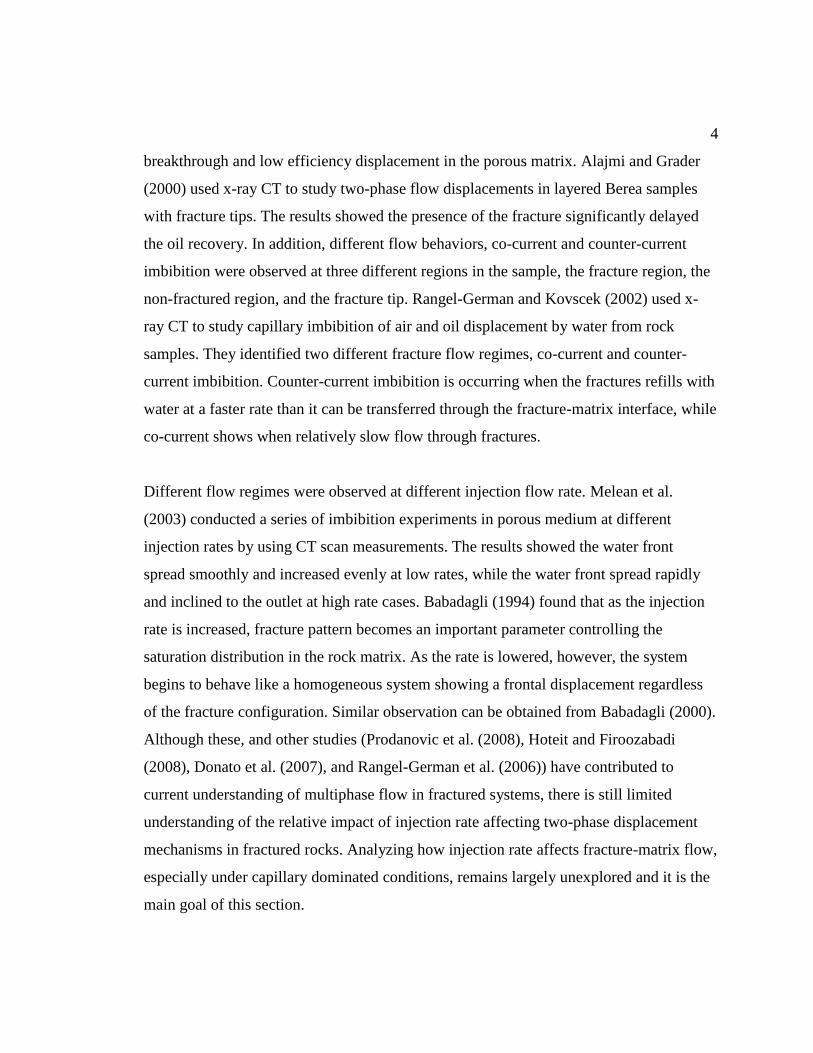
with viscous oil before starting brine injection. Figure 3-3 presents average saturation

changes as a function of time for all case. These saturations were averaged over the entire

sample, including fracture and rock matrix. In Figure 3-3, we can see the difference in

water saturation as a function of time and pore volume injected (PVI) for the three fluid

pairs under consideration. Since the existence of initial water saturation (Swi=0.1225) in

set 2, air-brine, initial saturations for set 2 is higher than set 1 and set 3 as shown in blue

diamond of Figure 3-3-top. In order to compare these saturation curves under the same

start point, pore volume injected (PVI) for set 2 was extrapolated to zero, as shown in

Figure 3-3-bottom. The results show that early time behavior is nearly identical for set1

and set 2, because this is controlled by the injection rate that has been specified as 4

mL/hr. After around 0.4 PVI, set 2 begins to separate from set 1 and reaches maximum

water saturation at an earlier time. In addition, set 2 increases as a straight and overlaps

the line of constant imbibion rate implying water saturation increases as a constant rate.

While for set 3, water saturation is negligible during the first 700 minutes of injection,

and increases up to 0.1 after 4000 minutes of continuous injection. The increment in

water saturation from set 1 and set 2 is much faster, displaying the influence of viscous

forces.

24

Figure 3-3: Average water saturation as a function of time and PVI for different fluid pairs.

0

0.1

0.2

0.3

0.4

0.5

0.6

0.7

0.8

0.9

1

0 200 400 600 800 1000 1200 1400 1600 1800 2000 2200 2400 2600 2800 3000 3200 3400 3600 3800 4000 4200 4400 4600

Av

era

ge

wa

ter s

atu

ra

tio

n

Time, min

Set 1, kerosene-brine

Set 2, air-brine

Set 3, viscous oil-brine

0

0.1

0.2

0.3

0.4

0.5

0.6

0.7

0.8

0.9

1

0 1 2 3 4 5 6 7 8 9 10 11 12 13 14 15 16 17 18 19 20

Av

era

ge

wa

ter s

atu

ra

tio

n


Constant imbibiton rate


Set 2, air-brine


25

The time progression of water saturation maps corresponding to three fluid pairs are

presented in Figure 3-4. Dark blue represents regions saturated with kerosene (Sw=0.0),

red represents regions saturated with water (Sw=1.0), and intermediate colors represent

the co-existence of kerosene and water. A late water breakthrough time, 0.54 PVI (135

minutes), is observed in set 2 (the case of water displacing air), while an early

breakthrough time, 0.03PVI (10 minutes), is observed in set 1 (the case of water

displacing kerosene). In addition, a co-current flow mechanism can be observed in set 2

where water and air toward a same direction, while a counter-current flow mechanism

where water and kerosene moving in an opposite direction was observed in set 1. This is

because a relative smaller viscosity ratio and higher interfacial tension in set 2 (the case

of water displacing air) than that in set 1 (the case of water displacing kerosene) that

makes injected water more easily flow from the fracture into the matrix; thus delaying

water breakthrough time and displaying as co-current flow mechanism. In addition, in

set 2, fracture-matrix transfer mechanism switches from co-current to counter-current

imbibition after water breakthrough, thus limiting additional recovery of the resident fluid

phase as shows in Figure 3-3 (after 135 minutes) and Figure 3-3 (after 0.54 PVI). That is

consistent with our knowledge that co-current imbibition can be a more efficient

displacement than counter-current flow (Pooladi-Darvish and Firoozabadi (2000)). In set

3, there is only a little increase in water saturation in the neighborhood of the fracture for

the first 300 minutes; however, none in the matrix. After 1440 minutes, the brine starts to

accumulate in the fracture, represented by the red shades. Under this flowing condition,

there is no evident matrix-fracture transfer or imbibitions into the rock matrix. The oil in

the fracture is displaced by brine due to forced injection.

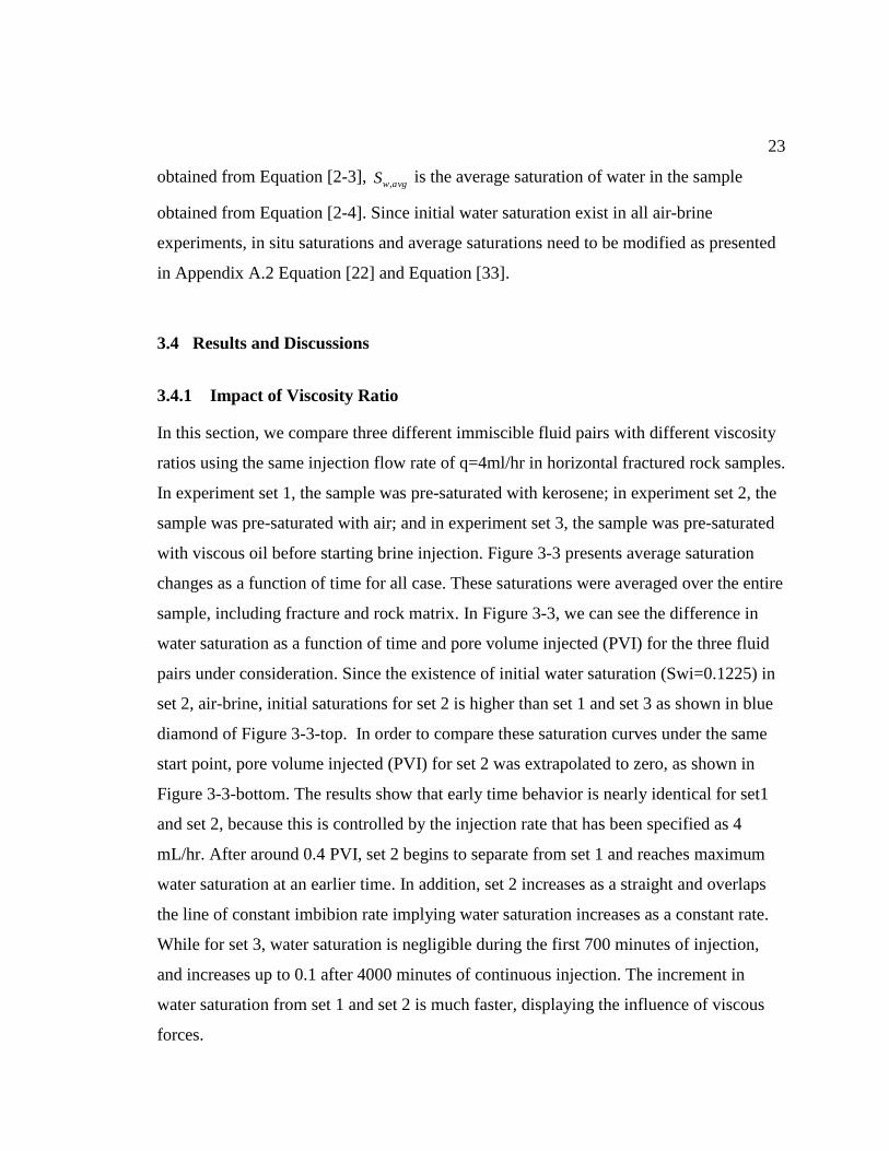
Close examination of Figure 3-5 reveals similar observation through vertical saturation

profiles. These vertical saturation profiles averaged over the central 6 mm of each CT

slice for three different fluid pairs. These profiles capture saturation changes with time in

the direction perpendicular to the fracture. For all experiments, continuous high water

saturation is observed at the center of the sample (0mm, or fracture location). In

26

experiment set 2, the saturations appear after 60 minutes of water injection, while a sharp

water saturation peak along the fracture is observed in the early time of set 1(t=20

minutes). That is consistent with a late water breakthrough time in experiment set 2 and

an early water breakthrough time in experiment set 1 observed in Figure 3-4. In set 3,

there is only a saturation peak in the fracture, and no water in the matrix implying that

capillary forces are not strong enough to drive brine into the matrix and displace the

resident viscous oil, thus making the overall process viscous dominated.

27

Figure 3-4: Sequence of water saturation maps obtained from CT scanning at 4mL/hr water injection rate for different fluid pairs.



4.90PVI0.79PVI0.58PVI0.38PVI0.27PVI0.17PVI0.10PVI0.03PVI

0.04PVI 0.13PVI 0.21PVI 0.34PVI 0.47PVI 0.99PVI 6.16PVI0.73PVI

Set 2, air-brine

4.21PVI0.75PVI0.54PVI0.38PVI0.27PVI0.17PVI0.10PVI0.03PVI

0.0

0.2

0.4

0.6

0.8

1.0

0.9

0.7

0.5

0.3

0.1

Sw

28

Figure 3-5: Vertical Saturation profiles perpendicular to the fracture and averaged over the central 6 mm of the sample, for different

fluid pairs.

-50

-40

-30

-20

-10

0

10

20

30

40

50

0 0.2 0.4 0.6 0.8 1

Dis

tan

ce f

rom

fractu

re (m

m)

Sw-Swi

T=10min

T=20min

T=60min

T=120min

T=180min

T=1440min

-50

-40

-30

-20

-10

0

10

20

30

40

50

0 0.2 0.4 0.6 0.8 1

Dis

tan

ce from

fract

ure (m

m)

Sw-Swi

-50

-40

-30

-20

-10

0

10

20

30

40

50

0 0.2 0.4 0.6 0.8 1

Dis

tan

ce from

fractu

re (m

m)

Sw-Swi

Set 2, air-brineSet 1, kerosene-brine Set 3, viscous oil-brine

Area of

interest

6 mm

29

3.4.2 Impact of Fracture Orientation

In this section, we compare five different fracture orientations in the case of water

displacing air using same injection flow rate q=4ml/hr as displayed in Figure 3-1,

including:

(1) horizontal fracture.

(2) vertical fracture flowing up.

(3) vertical fracture flowing down.

(4) diagonal fracture flowing up.

(5) diagonal fracture flowing down.

Figure 3-6 shows average water saturation as a function of pore volume injected (PVI)

for these five different fracture orientations. Once again, early time behavior is nearly

identical for all cases, because this is controlled by the injection rate that has been

specified as 4 mL/hr. After around 0.62 PVI, different cases start to separate from each

other. The cases of horizontal fracture and vertical fracture flowing down begin to

separate first and reach the lowest final saturation value at about 0.6-to-0.7 after 15 PVI.

On the contrary, diagonal fracture flowing up and vertical flowing up show later

breakthrough and higher ultimate saturation value after 15 PVI. The ultimate recovery

from these imbibition scenarios is primarily controlled by breakthrough time, when the

flow mechanism switches from co-current to counter-current, thus limiting extended

recovery of the resident fluid phase.

The time progression of water saturation maps corresponding to these five fracture

configurations are presented in Figure 3-7. A co-current flow mechanism prevailed in all

cases when displacing a non-wetting gas phase confirming previous observation in

Chapter 3.3.1 (impact of viscosity ratio) that co-current flow dominates in the case of

water displacing air due to a relative smaller viscosity ratio and higher interfacial tension.

In addition, the water front in the matrix is moving faster than that in the fracture, which

30

Figure 3-6: Average water saturation as a function of pore volume injected (PVI) for different fracture orientations.

0

0.1

0.2

0.3

0.4

0.5

0.6

0.7

0.8

0.9

1

0 1 2 3 4 5 6 7 8 9 10 11 12 13 14 15 16 17 18 19 20 21

Aver

age

wate

r sa

tura

tion


Constant injection rate (q=4mL/hr)

Vertical flowing down

Diagonal flowing down

Horizontal

Diagonal flowing up

Vertical flowing up

31

Figure 3-7: Sequence of water saturation maps obtained from CT scanning at 4mL/hr water injection rate for different fracture

orientations.

0.0

0.2

0.4

0.6

0.8

1.0

0.9

0.7

0.5

0.3

0.1

0.1PV >13.3P

V

1.00PV0.50PV0.2PV 0.40PV0.3PV

0

+90

-90

-45

+45

Sw

32

indicates that capillary force in the matrix is larger than that in the fracture. This

observation is evident as a shorter red line in the fracture zone within the imbibing front

in Figure 3-7.

The existence of rough-walled fractures and a relative faster moving rate of the water

front in the matrix than fracture also contribute to snap-off effects. There is direct

evidence of snap-off inside the fracture when the invading front in the matrix moves

ahead of the invading front in the fracture which leads to an air bubble was trapped

behind the water front in fracture zone as shown in Figure 3-8. This phenomena occurs

when the capillary pressure decreases or the radius of the curvature of the water (wetting-

phase fluid) increases and the water layers in the aperture start to swell and temporary cut

off the connection of air phase.

Figure 3-8: Saturation maps showing air (circular shadow) trapped in the fracture zone as

water injected time equals to 61 minutes.

Air bubble

33

Figure 3-9 shows snapshots of a generation of snap-off. An air bubble was trapped in the

fracture zone when water injected time equals to 61 minutes. However, this balance did

not hold for a long time. After one minute of continuous injection, this air bubble erupted,

and at the same time, it changed the shape of water front as water injected time equals to

62 minutes and the water front extended following this flow intermittency

Figure 3-9: Saturation maps showing air snap-off in the fracture.

The influence of fracture orientation resulting in different water breakthrough time can be

observed at PVI=0.4 (time=135minutes) where late water breakthrough can be

discovered in the case of diagonal fracture flowing up and vertical fracture flowing up. In

addition, higher water saturations represents in darker red can be observed behind

imbibing front in the case of diagonal fracture flowing up and vertical flowing up as

shown in Figure 3-7. This is because gravity slightly delays the progression of water

imbibing front and water breakthrough time, thus more water was accumulated behind

water front.

Similar observations are made from the vertical saturation profiles in Figure 3-10. A

higher water saturation value at the same PVI and slower water front evolving can be

observed in the Figure 3-10-right when PVI=0.2. In addition, a higher final water

saturation value can be observed in the fracture zone of Figure 3-10 right when

PVI=17.8.

(61min) (62min) (63min) (64min)(60min) (66min)(65min)

-90

34

Figure 3-10: Vertical Saturation profiles perpendicular to the fracture and averaged over the central 6 mm of the sample, in the case of

vertical fracture flowing down and vertical fracture flowing up.

-50

-40

-30

-20

-10

0

10

20

30

40

50

0 0.2 0.4 0.6 0.8 1D

ista

nce from

fractu

re (

mm

)Sw-Swi

0.10

0.20

0.30

0.40

0.50

1.00

17.8

-50

-40

-30

-20

-10

0

10

20

30

40

50

0 0.2 0.4 0.6 0.8 1

Dis

tan

ce from

fractu

re (

mm

)

Sw-Swi

0.10

0.20

0.30

0.40

0.50

1.00

13.3

Area of

interest6 mm

Fracture

location

PVI

Area of

interest6 mm

Fracture

location

PVI

Chapter 4

Numerical Analysis of Imbibition Front Evolution and History

Matching

Appropriate transport properties such as relative permeability and capillary pressures are

essential for successful simulation and prediction of multi-phase flow in such systems.

However, the lack of thorough understanding of the dynamics governing immiscible

displacement in fractured media limits our ability to properly represent their macroscopic

transport properties. In this study, an automated history matching approach proposed by

Basbug and Karpyn (2008) was implemented to generate representative matrix and

fracture relative permeability and capillary pressure curves Sequential saturation

distribution maps of brine displacing kerosene at low injection rate (4mL/hr) presented in

Chapter 2 were used as matched data. These optimized curves were then validated with

previous experimental data at higher water injection rate (40mL/hr) condition. Sensitivity

analyses were performed in order to study the effects of transport properties and

boundary effects on oil displacement and water front evolution. Through this study,

significant insight is provided for transport properties on the water front progression in

fractured permeable systems under capillary dominated conditions.


Transport properties such as permeability and capillary pressure are important for

successful description of fluid displacement processes (De la Porte et al. (2005)).

Numerous papers had proposed techniques for estimation of relative permeability and

capillary pressure curves for both matrix and fracture by using experiments or simulation

models. Heaviside et al. (1983) determined representative relative permeability and

capillary pressure curves using both steady-state and unsteady-state experiments as well

as numerical modeling. Firoozabadi and Hauge (1990) proposed a phenomenological

36

model to relate the fracture capillary pressure to saturation. El-Khatib (1995) developed a

modified J-function for calculating capillary pressure. Mohamad Ibrahim and L.F.

Koederitz (2001) presented a relative permeabilty prediction model from two phase

steady-state and unsteady-state experiment data. Bertels et al. (2001) developed an

experimental technique to measure and compute fracture aperture distribution, capillary

pressure, and relative permeability in fractured rocks using X-Ray CT scanning. Li

(2008) and Li and Horne (2010) generated a correlation between resistivity index with

relative permeability and capillary pressure data.

Kruger (1961) first applied history matching technique to calculated the areal

permeability distribution of the reservoir. Archer and Wong (1973) and Chavent et al.

(1980) applied similar approach to obtain relative permeability as well as capillary

pressure curves curves from experimental data. With the improvement of technology, this

technique becomes feasible to obtain permeability and capillary pressures curves. Chen et

al. (2005) developed optimization code based on Levenberg-Marquardt algorithm and

coupled it with a commercial reservoir simulator to match well test data and obtain

relative permeability curves. Basbug and Karpyn (2008) proposed a history matching

approach can automated determine both matrix and fracture relative permeability and

capillary pressure curves using B-spine equations. Angeles et al. (2010) developed

history matching model for relative permeability curves and capillary pressure curves

using field test data including resistivity, pressure and flow rates.

In order to accurately simulate and predict fluid transport behavior through fractured

systems, a thorough understanding of the variables that affect fluids transport through

fractures is necessary. Al-Wadahi et al. (2000) and Li (2003) applied of history matching

technique to investigate three phase counter-current flow mechanism. Similar study was

done by Alajmi (2003) to investigate the influence of a fracture tip on two-phase flow

displacement processes. Or (2008) indicated key factors shaping the displacement front

morphology, including fluid velocity, density and viscosity ratios, interfacial tensions,

37

and pore size distribution of the porous medium. Tavassoli et al. (2005a, b) proposed an

approximate analytical approach to analyze capillary force counter-current imbibitions in

both strongly and weak water-wet systems to assist dual-porosity modeling of flow in

fractured reservoirs. Rangel-German and Kovscek (2005) found that relative permeability

for fractured rocks with impermeable matrices are different from those for fractured

porous rocks. Relative permeability curves for fractures not interacting with granular

matrices are represented by X-type functions, while relative permeability for fractures

interacting with porous matrices do not necessary exhibit X-type behavior. The shape of

this function is controlled by injection flow rate, fracture aperature and the imbibition

potential of the rock.

However, analyzing the relationship between transport properties and water font

morphology especially under capillary dominated condition within fractured system,

remains largely unexplored, and is the main goal of this section. Results from this work

help visualize the impact of transport properties on the water front progression and, at the

same time, provide detailed quantitative information for the simulation and prediction of

multiphase flow in fractured permeable systems.

38

4.2 Automated History Matching Approach

History matching is a technique that adjusts simulation parameters until they are able to

reproduce the "history" of the modeled system. In this study, an automated history

matching approach proposed by Basbug and Karpyn (2008) was implemented and to

execute this matching approach. This code was developed under MATLAB® 2006b with

the optimization algorithm and coupled with the commercial reservoir simulator. The B-

spline functions used for determining relative permeability curves and C++ programming

code used for extracting saturation data from the simulator output results were replaced

by modified Brooks and Corey equations and a MATLAB®

subroutine code to simplify

and accelerate simulation speed.

A schematic diagram of automated history matching approach is illustrated in Figure 4-1.

The process starts with a reasonable initial guess of rock and fluid properties including

relative permeability and capillary pressure. The black oil module (IMEX (2009)) of a

commercial reservoir simulator (CMG) were use to run the simulation. Saturation

distribution were then extracted from the output results and compared with the

experimental data. Matrix and fracture relative permeability and capillary pressure curves

were then updated with a large-scale optimization algorithm (Trust-Region Method) if

the difference between experimental and simulation results did not fall within prescribed

error bounds. Large-scale optimization (Trust-Region Method) is an algorithm that

minimizes the least-squares objective function, J is implemented for adjusting. The

objective function is given by:

2

,,,

exp

,,,,,, ),(

tzyx

tzyxcr

cal

tzyx SPkSJ .................................................................................[4-1]

where cal

tzyxS ,,, is the saturation results calculated from simulation, while exp

,,, tzyxS is that

obtained from previous experiment.

39

Figure 4-1: Schematic diagram of history matching approach (Basbug and Karpyn

(2008)).

Initialization

Prepare

Input

Files

Initialize

Control

Parameters

Define

Flow

Properties

No

Large- scale Optimization

Prepare

New Input

File

Adjust

Control

Parameters

Re-define

Flow

Properties

Simulation

Run

Reservoir

Simulator

Determine

Saturation

Distribution ( Scal)

Convergence

Convergence

Check

J=∑(Scal-Sexp)^2

Report

Reservoir Flow

Properties

Yes

Basbug and Karpyn (2008)

40

The dimension of the experimental work in Chapter 2 was 485 485 pixels with the

resolution approximate 0.205mm (105mm/512). An up-scaling scheme was applied to

increase speed on both simulation and optimization process. For that purposes,

experimental data (saturation images) was up-scaled by a factor of 5 in each direction

using the arithmetic average. This factor is based on the fracture aperture resolution

suggested by Glass et al. (1998), and correlation length suggested by Keller (1998)).

After up-scaling scheme, simulation model dimension became 97 97 pixels with

approximate resolution 1.025mm (525 mm/512). This dimension was also applied to

following simulations including sensitivity analysis, automatic history matching approach

and predicted simulation studies.

The shape of the modeled system is a circular disk with diameter of approximate

99.463mm (50925 mm/512) and thickness of 10 mm. A continuous fracture layer is

positioned along in the center of the simulation model. The initial water saturation was

zero before starting water injection. We used constant flow rate inlet, 4mL/hr and

constant pressure outlet along with no flow boundary condition for the entire model. The

inlet and outlet were located at start and end of the fracture layers respectively.

Porosity distributions were extracted from experimental work in Chapter 2 and up-scaled

by a factor of 5 in each direction by using the arithmetic average.

Absolute permeability, k in each pixel was obtained from equation Timur’s correlation

(Timur (1968)), given by:

2

4.4

136.0wirrS

k

………………………………………………………….………… [4-2]

where is the pixel porosity of the rock sample (percentage) obtained from experimental

work in Chapter 2, and Swirr is the irreducible water saturation (fraction).

41

Table 4-1 presents a summary of porosity and permeability values used in the present

simulation model. Relative permeability and capillary pressure curves are defined with

modified Brooks and Corey equation (Lake (1989)), given by

Nw

wn

o

wrw SkSkrw)( ………………………………………………………………… [4-3]

No

wn

o

wro SkSkro

1)( ..………………......………..…………………………....…..... [4-4]

5.0)(

wn

cewc

S

PSP .……………….........………………………….…………....…...... [4-5]

wirror

wirrwwn

SS

SSS

1…………………………………………………………………… [4-6]

where wS is water saturation, rk is relative permeability, cP is capillary pressure,

wirrS and orS , were irreducible water saturation and residual oil saturation; end-point

relative permeabilities are identified with the superscript symbol “ o ” obtained from

perious steady-state relative permeability experiment. on and wn are Corey exponent to oil

and water respectively. ceP is capillary entry pressure.

Table 4-1: Rock properties assigned to fracture and matrix in simulation model.

Property Value

Fracture permeability [md] 5000

Average matrix permeability [md] 76.5

Fracture porosity [fraction] 0.3262

Matrix porosity [fraction] 0.2273

42

4.3 Sensitivity Analysis

To explore the sensitivity of imbibition front development to fracture/matrix transport

properties, we have constructed a series of test cases including sensitivity to matrix

relative permeability as well as matrix and fracture capillary pressure curves according to

the following case studies. All modified transport properties are listed in Table 4-2.

Case A: reference case.

We used base-case transport properties provided in Figure 4-2. Model dimensions,

porosity and absolute permeability distributions, flowing conditions and fluid properties

were as presented in Chapter 4.2 (page 41 through 43).

Figure 4-2: Matrix and fracture relative permeability curves (left) and capillary pressure

curves (right) used in sensitivity analysis case A.

Table 4-2: Lists of investigated parameters in sensitivity analysis cases.

Case Corey exponent

oil (no)

Corey exponent

water (nw)

End-point relative

permeability (korw)

Matrix capillary entry

pressure (Pce)

A 8 2.5 0.077 24.5

B 2 2.5 0.077 24.5

C 8 4 0.5 24.5

D 8 2.5 0.077 3.8

00.10.20.30.40.50.60.70.80.9

1

0 0.2 0.4 0.6 0.8 1

kr

Sw

kro (matrix)krow (matrix)kro (fracture)krow (fracture)

0

5

10

15

20

25

30

35

40

0 0.2 0.4 0.6 0.8 1

Pc

(psi

)

Sw

matrix

fracture

43

Case B: sensitivity to relative permeability to oil in the rock matrix.

To investigate the sensitivity of front evolution to matrix oil relative permeability ( rok ),

we increased relative permeability to oil by decreasing Corey exponent oil ( on ), to

compare cases A ( 8on ) and B ( 2on ), see Figure 4-3.


for sensitivity analysis cases A, B.

Case C: sensitivity to relative permeability to water in the rock matrix.

To investigate the sensitivity to matrix relative permeability to water ( rwk ), we increased

water relative permeability by Corey exponent water ( wn ) and increasing end-point

relative permeability (o

rwk ), to compare cases A ( 5.2wn , 077.0o

rwk ) and C ( 4wn ,

5.0o

rwk ), see Figure 4-4.

00.10.20.30.40.50.60.70.80.9

1

0 0.2 0.4 0.6 0.8 1

kro

Sw

kro (case A)

kro (case B)

krow (cases A, B)

0

5

10

15

20

25

30

35

40

0 0.2 0.4 0.6 0.8 1P

c (p

si)

Sw

matrix (cases A, B)

fracture (cases A, B)

00.10.20.30.40.50.60.70.80.9

1

0 0.2 0.4 0.6 0.8 1

krw

Sw

kro (cases A, C)

krow (case A)

krow (case C)

0

5

10

15

20

25

30

35

40

0 0.2 0.4 0.6 0.8 1

Pc

(psi

)

Sw

matrix (cases A, C)

fracture (cases A, C)

44


for sensitivity analysis cases A, C.

Case D: sensitivity to capillary pressure contrast between matrix and fracture.

To investigate the sensitivity to capillary pressure contrast between matrix and fracture,

we decrease capillary entry pressure ( ceP ) in the fracture to compare cases A ( 5.24ceP )

with D ( 8.3ceP ), see Figure 4-5.


for sensitivity analysis cases A, D.

Simulation results of imbibition front evolution in fractured sandstone were compared

and analyzed based of average water saturation (Figure 4-6), water saturation maps as a

function of time (Figure 4-7), and water saturation profiles perpendicular to the fracture

(Figure 4-8). Figure 4-6 presents average saturation changes as a function of time for all

cases. These saturations were averaged over the entire sample, including fracture and

rock matrix. Early time behavior is nearly identical for all cases, because this is

controlled by the injection rate that has been specified as 4 mL/hr. After around 80

minutes of injection, each test case begins to separate from the reference case A. Cases B,

C and D reach higher water saturation faster, and thus higher oil displacement, than case

A, implying more mobile oil and water phases inside the modeled system. Notice that an

increase in matrix relative permeability (cases B and C) or capillary pressure contrast

between matrix and fracture (case D), can lead a faster oil displacement rate. At a water

saturation of about 0.56, oil displacement becomes negligible in cases A, C and D;

00.10.20.30.40.50.60.70.80.9

1

0 0.2 0.4 0.6 0.8 1

kr

Sw

kro (cases A, D)

krow (cases A, D)

0

5

10

15

20

25

30

35

40

0 0.2 0.4 0.6 0.8 1

Pc

(psi

)

Sw

matrix (cases A, B)

fracture (cases A, B)

fracture (case D)

45

however, in case B, saturation keeps increasing until 0.8, which is consistent with a larger

mobile region in the transport properties specified for case B.

Figure 4-6: Average water saturation as a function of time for sensitivity cases A, B, C

and D.

Figure 4-7 shows time progressions of water saturation (Sw) maps for cases A through D.

Red represents regions saturated with water (Sw=1.0), dark blue represents regions

saturated with kerosene (Sw=0.0), and intermediate represent the co-existence of

kerosene and water. In Figure 4-7, case A, base case, an early water breakthrough was

observed. Under this flowing condition, the fractures refills with water at a faster rate

than it can be transferred through the fracture-matrix interface, confirming similar

experimental observations found in the literature (Rangel-German and Kovscek (2002)).

Simultaneously, counter-current imbibition is occurring in the water invaded zone as oil

is expelled from the matrix into the fracture. As time progresses, the imbibition front

moves away from the fracture, and water accumulation becomes evident in the fracture

zone in red, supporting the fact that the rate of capillary dispersion through the matrix is

low compared to the rate of injection.

0

0.1

0.2

0.3

0.4

0.5

0.6

0.7

0.8

0.9

1

0 250 500 750 1000 1250 1500

Sw

Time(min)

case A

case B

case C

case D

46

Figure 4-7: Sequence of water saturation maps at 4mL/hr water injection rate for

sensitivity cases A, B, C and D.

In cases B and C, where oil and water matrix relative permeability curves were increased

relative to the reference case A, early water breakthrough and counter-current flow

mechanism were also observed. However, a higher final water saturation can be

observed in case B, as time equals to 1430 minutes. This observation confirm a previous

finding in Figure 4-6, due to a larger mobile region for oil phase in the transport

properties specified for case B, final water saturation can keep increasing until 0.8.

10min 80min 170min 1430min

Case A


Case B


Case C


Case D

0.0

0.2

0.4

0.6

0.8

1.0

0.9

0.7

0.5

0.3

0.1

Sw

47

In case C, where matrix relative permeability to water has been increased, we observe a

faster water front extension as it spreads away from the fracture when time equals both

80 and 170 minutes. This is because of the wider mobile range for the water phase in the

transport properties specified for case C, which make the injected water more mobile at

low saturation. However, because matrix relative permeability to oil in cases A and C, the

increased matrix relative permeability to water can only enable the water front to extend

farther into the matrix instead of increasing the average water saturation in the sample.

In case D, there is a significant difference in the shape of the imbibition front due to

increased capillary pressure contrast between matrix and fracture. We also observe a

delayed water breakthrough in case D. This form of imbibition front evolution is

characterized by an early period of co-current displacement until water breakthrough,

followed by counter-current imbibition. In this case, due to higher capillary pressure

contrast between fracture and matrix, injected water is more easily derived from the

fracture, and thus delaying its breakthrough time, presenting an inclined shape of water

fronts, and a higher water saturation value behind water front as shown in yellow as 80

minutes of Figure 4-7 case D.

Further quantitative examination of saturation changes for cases A through D is presented

in Figure 4-8. These are vertical saturation profiles average over the central 6 mm of the

simulation model, which capture saturation distribution at 80 minutes of injection, in the

direction perpendicular to the fracture. As shown in Figure 4-6, all cases reach almost the

same average saturation value after 80 minutes of injection. Under this time frame, an

increased oil relative permeability in the matrix (case B) shares a similar vertical

saturation profile with the reference case A, as shown in Figure 4-8, representing a

similar imbibition rate from the fracture into matrix.

48


the central 6 mm of the simulation model, q=4mL/hr at time=80 minutes for sensitivity

analysis cases A, B, C and D.

However, an increase in water relative permeability (case C) tends to lead a much

broader water front progression, and consequently decreases the amount of water

saturation in the fracture zone. In addition, this extension changes saturation gradient,

causing a drastic drop in saturation across the water front. The same phenomenon is

demonstrated in the plot presented in Figure 4-9, where the loss of color contrast behind

the water front was observed with increasing the water front progression to matrix system

in case C. In case D, the increased capillary pressure contrast between matrix and fracture

creates an even broader water front, which is consistent with early observations of higher

oil displacement rate and inclined shape of water fronts in Figure 4-7. It is therefore

-50

-40

-30

-20

-10

0

10

20

30

40

50

0 0.2 0.4 0.6 0.8 1

Dis

tan

ce from

fractu

re (m

m)

Sw

case A

case B

case C

case D

Area of

interest

6 mm

49

proved that either water relative permeability or capillary pressure contrast can increase

mobility of water phase, and thus influence the speed of water front extension, while the

relative permeability to oil primarily controls residual saturations at the end of the

displacement process. The balance of capillarity and relative permeabilities also has a

significant impact of the shape of the invasion front, resulting in periods of co-current

and counter-current imbibition.

4.4 History Matching Results and Validation

The purpose of this section is to determine the representative transport properties using

the proposed automated history matching method, and hence could be readily adapted for

its application to the analysis of additional predictive scenarios. A sequential saturation

distribution maps at low water injection rate (4mL/hr) was used as matched data to

generate representative relative permeability and capillary pressure curves. Based on the

observations from the experiments and sensitivity analysis, an appearance of early water

breakthrough and counter-current imbibition should be observed throughout the

simulation. Average saturation as a function of time, spatial saturation profiles, and visual

inspection of imbibition front are used as additional agreement criteria to generate a

robust history matching result. These optimized curves were then validated with previous

experimental data at higher water injection rate (40mL/hr) condition. Three further

simulations were used to investigate the effect of homogeneity, heterogeneity and shape

of boundary condition on the imbibition front evolution.

Relative permeability and capillary pressure curves after history matching approach are

shown in Figure 4-9 and Figure 4-10. Figure 4-9 indicates that relative permeability curve

in fracture is larger than that in matrix, while capillary pressure in matrix is higher as

shown in Figure 4-10. The relative permeability ratio between oil and water phase

(kro/krw) is close to 0 as water saturation equals to 0.55 implying oil displacement rate

starts to slow down after that point. In addition, matrix relative permeability curves

50

intersect at a water saturation of 0.53, which is consistent with experimental observation

of a dynamic equilibrium between oil and water phases within the imbibed zone at

Sw=0.50-to-0.55. (Lee and Karpyn (2010)).

Figure 4-9: Matrix and fracture relative permeability curves obtained from history

matching method.

Figure 4-10: Capillary pressure curves on both matrix and fracture obtained from history

matching method.

0

0.1

0.2

0.3

0.4

0.5

0.6

0.7

0.8

0.9

1

0 0.1 0.2 0.3 0.4 0.5 0.6 0.7 0.8 0.9 1

kr

Sw

KrowKrwKrwfKrowf

0

5

10

15

20

25

30

35

40

0 0.1 0.2 0.3 0.4 0.5 0.6 0.7 0.8 0.9 1

Pc

(psi

)

Sw

Pcow

Pcowf

51

Figure 4-11 shows an independent validation of relative permeability curves obtained

from the history matching methods, against experimental measurements using steady-

state two-phase displacement in cylindrical cores. The curves obtained from the history

match are slightly lower than the experimental ones, which is attributed to the fact that

the steady-state displacement experiment took place is a co-current manner, while the

history matched results correspond primarily to counter-current flow. The difference in

the magnitude of co-current and counter-current relative permeabilities is consistent with

findings reported by Bourbiaux and Kalaydjian (1990).

Figure 4-11: Comparison of experimental and history matched relative permeability

curves.

A comparison of modeled and experimental saturation changes as a function of time and

pore volume injected reveal excellent agreement, as seen in Figure 4-12. A one-on-one

comparison of modeled and experimental saturation maps is presented in Figure 4-13,

and confirms the goodness of the proposed modeling methodology and the transport

properties derived from its implementation. Figure 4-14 also shows good agreement of

temporal vertical saturation profiles. The progression of the modeled imbibition front at

0

0.1

0.2

0.3

0.4

0.5

0.6

0.7

0.8

0.9

1

0 0.1 0.2 0.3 0.4 0.5 0.6 0.7 0.8 0.9 1

kr

Sw

Krow(history matching)Krw(history matching)Krow(Steady-state exp.)Krw(Steady-state exp.)

52

early time seems to be slightly ahead of the experimental front in Figure 4-14, which can

be explained through small differences in the continuity of the fracture zone and the

simplified representation of the fracture by a row of grid blocks having uniform

properties.

Figure 4-12: Comparison of experimental and modeled average water saturation as a

function of time at 4mL/hr water injection rate.

0

0.1

0.2

0.3

0.4

0.5

0.6

0.7

0.8

0.9

1

0 2 4 6 8 10 12 14 16 18

Sw

Pore Volume Injected

Exp.(q=4mL/hr)

Sim.(q=4mL/hr)

0

0.1

0.2

0.3

0.4

0.5

0.6

0.7

0.8

0.9

1

0 500 1000 1500 2000 2500 3000 3500 4000 4500 5000

Sw

Time(min)

Exp.(q=4mL/hr)

Sim.(q=4mL/hr)

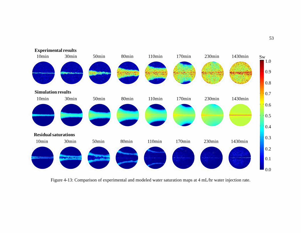
53

Figure 4-13: Comparison of experimental and modeled water saturation maps at 4 mL/hr water injection rate.


Simulation results

0.0

0.2

0.4

0.6

0.8

1.0

0.9

0.7

0.5

0.3

0.1

Sw


Residual saturations

Experimental results


55

Figure 4-14: Comparison of experimental and modeled vertical saturation profiles


q=4mL/hr.

-50

-40

-30

-20

-10

0

10

20

30

40

50

0 0.2 0.4 0.6 0.8 1

Dis

tan

ce f

rom

fra

ctu

re

(mm

)

Sw

10min(Exp.)

80 min(Exp.)

170 min(Exp.)

1430min(Exp.)

10min(Sim.)

80 min(Sim.)

170 min(Sim.)

1430min(Sim.)

Area of

interest

6 mm

55

An additional test of the validity of the modeled system and transport properties was

performed by predicting the evolution of the imbibition front and saturation changes at a

higher injection rate, for which we also had experimental data. This data set at higher

injection rate was not presented to the model during the history match process, but rather

used to assess the accuracy of the predictions. When using the matched transport

properties to predict imbibition front evolution at a higher injection rate of 40mL/hr, the

prediction still showed excellent agreement as displayed in Figure 4-15 through Figure

4-17.

Simulation results from different injection rates, in Figure 4-12 and Figure 4-15, show

that higher-rate curve (q=40mL/hr) reaches higher water saturation, and thus higher oil

displacement, at the expense of more pore volumes injected. The rate of injection is also

responsible for the shape of the imbibing front, which is farther away from the fracture

inlet than the outlet, as shown in Figure 4-16. This observation is less pronounced when

the rate of injection is reduced, as shown in Figure 4-13. In addition, for approximately

the same pore volume injected, that is 10min (0.36PVI) at high-rate case and 110min

(0.33PVI) at low-rate case, we observe a much larger imbibed region in the low-rate case.

This implies low injection rate (4mL/hr) allows a more effective spreading of water for

the same volume injected.

Further quantitative examination of saturation changes can be obtained from vertical

saturation profiles, Figure 4-14 and Figure 4-17. For both simulation results, continuous

high water saturation is observed in the center of the sample, where the fracture is

located. The most noticeable differences between these two vertical profiles are: (1) the

speed at which the water front moves away from the fracture, and (2) the change in

saturation as moves away from the fracture. Figure 4-14 shows a gradual saturation

change at the front, while there is a relative sharp drop in saturation across the water front

in Figure 4-17. Furthermore, water saturations remain in the 0.50-to-0.55 range within the

imbibed zone, which is consistent with the previous experimental results.

56

Figure 4-15: Comparison of experimental and predicted average water saturation as a

function of time at 40mL/hr water injection rate.

0

0.1

0.2

0.3

0.4

0.5

0.6

0.7

0.8

0.9

1

0 10 20 30 40 50 60

Sw

Pore Volume Injected

Exp.(q=40mL/hr)

Sim.(q=40mL/hr)

0

0.1

0.2

0.3

0.4

0.5

0.6

0.7

0.8

0.9

1

0 250 500 750 1000 1250 1500

Sw

Time(min)

Exp.(q=40mL/hr)

Sim.(q=40mL/hr)

57

Figure 4-16: Comparison of experimental and predicted water saturation maps at 40 mL/hr water injection rate.

0.0

0.2

0.4

0.6

0.8

1.0

0.9

0.7

0.5

0.3

0.1

SwExperimental results


Simulation results


58

Figure 4-17: Comparison of experimental and predicted vertical saturation profiles


q=40mL/hr.

.

-50

-40

-30

-20

-10

0

10

20

30

40

50

0 0.2 0.4 0.6 0.8 1

Dis

tan

ce f

rom

fra

ctu

re (m

m)

Sw

10min(Exp.)

40min(Exp.)

90min(Exp.)

1440min(Exp.)

10min(Sim.)

40min(Sim.)

90min(Sim.)

1440min(Sim.)

Area of

interest

6 mm

59

4.5 Predictive Cases

Having established a solid level of confidence in the modeled system, relative to its

experimental counterpart, allowed us to design additional predictive scenarios to explore

the influence of matrix homogeneity/heterogeneity and boundary shape on the response

of the imbibition front. To investigate the influence of matrix homogeneity/heterogeneity

on water front evolution, we compare three different porosity and permeability

distributions as cases A, E and F with the same the transport properties provided in

Figure 4-9 and Figure 4-10. This investigation can also help to explain the mismatching

of faster water front evolving at early time in Figure 4-14. In circular systems, the water

front hits outer boundaries faster in the inlet than the outlet.

Case A: reference case.

The average porosity and permeability are the same in all additional predictive cases.

Their standard deviation in porosity and permeability are also listed in Table 4-3.

Case E: as homogeneous systems.

In case E, a single porosity (0.2273) and permeability (76.5 md) value were applied for

entire modeled system except the fracture zone. A more uniform porosity and

permeability distribution is expected to obtained than that in case A.

Table 4-3: Standard deviation of porosity and permeability for cases A, E, F and G.

Case Standard deviation of

Porosity(mean=0.2273)

Standard deviation of

Permeability(mean=76.5mD)

A 0.04 45.02

E 0.00 0.00

F 0.09 169.83

G 0.04 45.02

60

Case F: as heterogeneous systems,

In case F, matrix porosity variations were increased according to following equation:

avgavgpixnewpix a )(_

where a is deviation factor (a=3), avg and pix are average and pixel porosity

respectively. Timur’s correlation (Timur (1968)) was used to obtain an absolute

permeability value after a porosity distribution map was created. Figure 4-22 displayed

porosity and permeability distributions for predictive case F. Figure 4-18 displays

porosity and permeability histograms for cases A and F. Porosity and permeability in

both cases shape as normal distribution according to Anderson-Darling Normality test

(Anderson and Darling (1951)), while reference case A presents as a more sorted system

than case F.

Case G: as square boundaries.

To study the effects of boundary shape on imbibing front inclination, which is away from

the fracture inlet than the outlet as shown in Figure 4-13 and Figure 4-16, in case G, we

change circular boundary as a square boundary using the same rock and fluid properties

of reference case A. This additional case study can help to understand the effects of

boundary shape on imbibing front inclination.

Figure 4-18: Matrix porosity (left) and permeability (right) histograms for cases A and F.

0%

5%

10%

15%

20%

25%

30%

0.00 0.04 0.08 0.12 0.16 0.20 0.24 0.28 0.32 0.36 0.40

%

porosity

case A

case F

0%

5%

10%

15%

20%

25%

30%

0 40 80 120 160 200 240 280 320 360 400

%

permeability (mD)

case A

case F

61

Figure 4-19 presents average saturation changes as a function of time for cases A, E, F

and G. The results show oil displacement rate is nearly identical for cases A, E and G

throughout the entire simulations. Close examination of case E, the homogeneous system,

shows that saturations begin to separate from case A and increase slightly faster after

around 100 minutes of water injection. Further increments become negligible after 400

minutes and reach a final water saturation of about 0.56. This can be explained by the fact

that rock properties of the reference case A are close to homogeneous. However, in case

F (heterogeneous system), saturations separate from case A after 30 minutes injection,

and increase at a slower rate with respect to case A. After 1400 minutes of injection,

saturation reaches a final saturation value of 0.55. It indicates the increase matrix

heterogeneity decreases oil displacement rate. It also confirms the previous observation

that the displacement rate is mainly controlled by relative permeabilities. Furthermore, in

case G, we change the circular boundaries to square boundaries. Saturation distributions

obtained from case G are nearly identical to the reference cases A, implying that the

shape of the boundaries has low effect on oil displacement under capillary dominant

condition.

Figure 4-19: Average water saturation as a function of time at 4mL/hr water injection rate

for cases A, E, F and G.

0

0.1

0.2

0.3

0.4

0.5

0.6

0.7

0.8

0.9

1

0 500 1000 1500

Sw

Time(min)

case Acase Ecase Fcase G

62

Similar observations are made from the time progressions of water saturation maps in

Figure 4-20. Case E, the homogeneous system, shows a slightly faster water front

extension respect to reference case A, while an unsmooth and slower water front

progression was observed in case F, the heterogeneous systems. This result extends our

previous conclusions that the reason for the mismatch of water front at early time in

Figure 4-14 is not limited to the continuity of the fracture zone and the simplified

representation of the fracture. An up-scaling scheme for the simulation model could

create a smooth property distribution and a more homogeneous system that can contribute

to the speed of water front evolution. In addition, the system with square boundary (case

G), shows similar results to the system with circular boundary (case A), confirming that

the rate of injection is responsible for the shape of the imbibing front, and this effect is

less pronounced when the rate of injection is reducing. Under capillary-dominant

counter-current flow regimes, the shape of the boundary has a minimal effect on shape of

imbibing front evolution.

63

Figure 4-20: Predicted sequence of water saturation maps at 4mL/hr water injection rate for cases A, E, F and G.

30min 50min 80min 110min 170min 230min 1430min



10min


10min

10min

0.0

0.2

0.4

0.6

0.8

1.0

0.9

0.7

0.5

0.3

0.1

Sw

Case A

Case E

Case F

Case G

Chapter 5

Conclusions

Understanding and predicting the migration of fluids in fractured geologic systems is of

great importance in many geological applications, be it for remediation, recovery,

storage, or sequestration. In this study, we analyze the impact of injection rate, viscosity

ratio, fracture orientation and transport properties on recovery and imbibition front

evolution in fractured sandstone, under capillary dominated conditions. Results lead to

the following conclusions:

The higher injection flow rate (q=40mL/hr) shows higher oil recovery, at the

expense of more pore volumes injected to reach the ultimate oil recovery. A sharp

imbibing front is observed in the high-rate experiment, while a smoother

saturation gradient is observed at low rate. Water saturation in the imbibed zone

remains constant at around 0.50-to-0.55, suggesting a dynamic equilibrium in the

mobility of oil and water phases. We also describe the counter-current flow

mechanisms that are evident from the experimental results, and support our

observations on the evolution of saturation maps and profiles obtained in the

laboratory.

Co-current flow dominates in the case of water displacing air, while counter-

current flow dominates in the case of water displacing kerosene. Liquid-liquid (in

the case of water displacing kerosene) and gas-liquid (in the case of water

displacing air) imbibition results show significant differences in the shape of the

imbibing front, breakthrough time, and saturation profiles. Capillary forces are

significantly hindered in the case of water displacing viscous oil when the

viscosity of the displaced phase increases, thus making the overall process viscous

dominated.

65

The influence of fracture orientation on the shape of the imbibing front, and

ultimate recovery, was minimal for the time- and length-scales considered in this

investigation. However, the varying relevance of gravity at different fracture

inclinations still causes changes in water saturation distribution behind the

imbibing front, and breakthrough time. Water breakthrough also switches the

fracture-matrix transfer mechanism from co-current to counter-current, thus

limiting additional recovery of the resident fluid phase. In addition, there is direct

evidence of snap-off inside the fracture when the invading front in the matrix

moves ahead of the invading front in the fracture.

Final saturation and ultimate displacement are most sensitive to relative

permeability ratio between oil and water phase. Relative permeability to water in

the matrix, capillary pressure contrast between matrix and fracture, and degree of

rock heterogeneity determine the speed and shape of imbibing front progression.

The balance of capillarity and relative permeabilities also has a significant impact

on the shape of the invasion front, resulting in periods of co-current and counter-

current imbibition. Fracture permeability, and capillary pressure contrast between

matrix and fracture dominate occurrence of water breakthrough. The impact of

boundary shape on imbibition front evolution was found to be minimal under the

evaluated flow conditions, which are dominated by capillary forces.

Additional experimental and numerical analyses in tight sands and shale are

required in the future which would be benefit to evaluate migration and trapping

of hydraulic fracturing leak-off under shut-in conditions.

References

Ajose, D., Mohanty, K.K.: Compositional Upscaling in Heterogeneous Reservoirs: Effect of Gravity, Capillary Pressure, and Dispersion. In: SPE Annual Technical Conference and Exhibition, Denver, Colorado, USA, 5-8 October 2003

Al-Wadahi, M., Grader, A.S., Ertekin, T.: An Investigation of Three-Phase Counter-Current Flow Using X-Ray Computerized Tomography and Neuro-Simulation Modeling. In: SPE Annual Technical Conference and Exhibition, Dallas, Texas, USA, 1-4 October 2000

Alajmi, A.F.: The Influence of a Fracture Tip on Two-Phase Flow Displacement Processes. Ph.D. , The Pennsylvania State University (2003)

Alajmi, A.F., Grader, A.S.: Analysis of Fracture-Matrix Fluid Flow Interactions Using X-Ray CT. In: SPE Eastern Meeting, Morgantown, West Virginia, 17-19 October 2000

Anderson, T.W., Darling, D.A.: Asymptotic Theory of Certain Goodness of Fit Criteria Based on Stochastic Processes. Annals of Mathematical Statistics 22(1), 143-143 (1951)

Angeles, R., Torres-Verdín, C., Hadibeik, A., Sepehrnoori, K.: Estimation of Capillary Pressure and Relative Permeability from Formation-Tester Measurements using Design of Experiment and Data-Weighing Inversion: Synthetic and Field Examples. Journal of Petroleum Science and Engineering (2010). doi:10.1016/j.petrol.2010.10.006

Archer, J.S., Wong, S.W.: Use of a Reservoir Simulator To Interpret Laboratory Waterflood Data SPE Journal 13(6), 5 (1973)

Babadagli, T.: Injection Rate Controlled Capillary Imbibition Transfer in Fractured Systems. In: SPE Annual Technical Conference and Exhibition, New Orleans, LA, USA, 25-28 September 1994

Babadagli, T.: Efficiency of capillary imbibition dominated displacement of nonwetting phase by wetting phase in fractured porous media. Transport in Porous Media 40(3), 323-344 (2000)

Basbug, B., Karpyn, Z.T.: Determination of Relative Permeability and Capillary Pressure Curves Using an Automated History-Matching Approach. Paper presented at the SPE Eastern Regional/AAPG Eastern Section Joint Meeting, Pittsburgh, Pennsylvania, USA, 11-15 October 2008

Berkowitz, B.: Characterizing flow and transport in fractured geological media: a review. Advance in Water Resources 25, 24 (2002)

Bertels, S.P., DiCarlo, D.A., Blunt, M.J.: Measurement of aperture distribution, capillary pressure, relative permeability, and in situ saturation in a rock fracture using computed tomography scanning. Water Resources Research 37(3), 649-662 (2001)

Bourbiaux, B.J., Kalaydjian, F.J.: Experimental Study of Cocurrent and Countercurrent Flows in Natural Porous Media Spe Reservoir Engineering 5(3), 361-368 (1990)

Carnes, P.S.: Effects of Natural Fractures or Directional Permeability in Water Flooding. In: SPE Secondary Recovery Symposium, Wichita Falls, Texas, 2-3 May 1966

Chavent, G., Cohen, G., Espy, M.: Determination of Relative Permeability and Capillary Pressure by Automatic Adjustment Method. In: SPE Annual Technical Conference and Exhibition, Dallas, Texas, USA, 21-24 September 1980

67

Chen, S., Li, G., Peres, A., Reynolds, A.C.: A Well Test for In-Situ Determination of Relative Permeability Curves In: SPE Annual Technical Conference and Exhibition, Dallas, Texas, USA, 9-12 October 2005

Committee on Fracture Characterization and Fluid Flow, N.R.C.: Rock fractures and fluid flow: contemporary understanding and applications. National Academy Press, Washington, D.C. (1996)

Crandall, D., Ahmadi, G., Smith, D.H.: Computational Modeling of Fluid Flow through a Fracture in Permeable Rock. Transport in Porous Media 84(2), 493-510 (2010). doi:DOI 10.1007/s11242-009-9516-9

Crawford, P.B., Collins, R.E.: Estimated Effect of Vertical Fractures on Secondary Recovery. Transactions of the American Institute of Mining and Metallurgical Engineers 201, 192-196 (1954)

De la Porte, J.J., Kossack, C.A., Zimmerman, R.W.: The Effect of Fracture Relative Permeabilities and Capillary Pressures on the Numerical Simulation of Naturally Fractured Reservoirs Paper presented at the SPE Annual Technical Conference and Exhibition, Dallas, Texas, USA, 9-12 October 2005

Ding, M., Kantzas, A.: Capillary number correlations for gas-liquid systems. Journal of Canadian Petroleum Technology 46(2), 27-32 (2007)

Donato, G., Lu, H.Y., Tavassoli, Z., Blunt, M.J.: Multirate-Transfer Dual-Porosity Modeling of Gravity Drainage and Imbibition. SPE Journal 12(1), 77-88 (2007)

El-Khatib, N.: Development of a Modified Capillary Pressure J-Function In: Middle East Oil Show, Bahrain, 11-14 March 1995

Farzaneh, S.A., Kharrat, R., Ghazanfari, M.H.: Experimental Study of Solvent Flooding to Heavy Oil in Fractured Five-Spot Micro-Models: The Role of Fracture Geometrical Characteristics. Journal of Canadian Petroleum Technology 49(3), 36-43 (2010)

Firoozabadi, A., Hauge, J.: Capillary-Pressure in Fractured Porous-Media. Journal of Petroleum Technology 42(6), 784-791 (1990)

Firoozabadi, A., Markeset, T.: An Experimental Study of Capillary and Gravity Crossflow Fractured Porous Media. In: SPE Annual Technical Conference and Exhibition, Washington, DC, 4-7 October 1992

Glass, R.J., Nicholl, M.J., Yarrington, L.: A modified invasion percolation model for low-capillary number immiscible displacements in horizontal rough-walled fractures: Influence of local in-plane curvature. Water Resources Research 34(12), 3215-3234 (1998)

Gu, Y.G., Yang, C.D.: The Effects of Capillary Force and Gravity on the Interfacial Profile in a Reservoir Fracture or Pore. Journal of Petroleum Science and Engineering 40(1-2), 77-87 (2003). doi:Doi 10.1016/S0920-4105(03)00104-9

Heaviside, J., Black, C.J.J., Berry, J.F.: Fundamentals of Relative Permeability: Experimental and Theoretical Considerations In: SPE Annual Technical Conference and Exhibition, San Francisco, California, USA, 5-8 October 1983

Hognesen, E.J., Olsen, M., Austad, T.: Capillary and gravity dominated flow regimes in displacement of oil from an oil-wet chalk using cationic surfactant. Energy & Fuels 20(3), 1118-1122 (2006). doi:Doi 10.1021/Ef050297s

Hoteit, H., Firoozabadi, A.: An efficient numerical model for incompressible two-phase flow in fractured media. Advances in Water Resources 31(6), 891-905 (2008). doi:DOI 10.1016/j.advwatres.2008.02.004

Ide, S.T., Jessen, K., Orr, F.M., Jr.: Storage of CO2 in saline aquifers: effects of gravity, viscous, and capillary forces on amount and timing of trapping. J. Greenhouse Gas Control 1, 481-491 (2007)

68

IMEX: Three-Phase Black Oil Simulator, User’s Guide. In. Computer Modeling Group (CMG), Calgary, (2009)

Karpyn, Z.T., Alajmi, A., Radaelli, F., Halleck, P.M., Grader, A.S.: X-ray CT and Hydraulic Evidence for a Relationship between Fracture Conductivity and Adjacent Matrix Porosity. Engineering Geology 103(3-4), 139-145 (2009). doi:DOI 10.1016/j.enggeo.2008.06.017

Karpyn, Z.T., Li, G., Grader, A.S., Halleck, P.M.: Experimental Conditions Favoring the Formation of Fluid Banks during Counter-Current Flow in Porous Media. Transport in Porous Media 62(1), 109-124 (2006). doi:DOI 10.1007/s11242-005-0617-9

Keller, A.: High resolution, non-destructive measurement and characterization of fracture apertures. International Journal of Rock Mechanics and Mining Sciences 35(8), 1037-1050 (1998)

Kruger, W.D.: Determining Areal Permeability Distribution by Calculations Journal of Petroleum Technology 13(7), 6 (1961)

Lake, L.W.: Enhanced oil recovery. Chapter 3, Prentice Hall Inc., Englewood Cliffs, NJ, USA (1989)

Lee, C.H., Karpyn, Z.T.: Experimental Investigation of Rate Effects on Two-phase Flow through Fractured Rocks Using X-Ray Computed Tomography. Paper presented at the 3rd International Workshop on X-Ray CT for Geomaterials New Orleans, Louisiana, USA, Mar. 1-3

Lefebvre du prey, E.: Gravity and Capillarity Effects on Imbibition in Porous-Media. Society of Petroleum Engineers Journal 18(3), 195-206 (1978)

Li, G.: History Dependent Modeling of Countercurrent Flow in Porous Media. Ph.D. , The Pennsylvania State University (2003)

Li, K.: A new method for calculating two-phase relative permeability from resistivity data in porous media. Transport in Porous Media 74(1), 21-33 (2008). doi:DOI 10.1007/s11242-007-9178-4

Li, K., Horne, R.N.: Correlation Between Resistivity Index, Capillary Pressure and Relative Permeability. In: Proceedings World Geothermal Congress 2010, Bali, Indonesia,, 25-29 April 2010

Melean, Y., Broseta, D., Blossey, R.: Imbibition fronts in porous media: effects of initial wetting fluid saturation and flow rate. Journal of Petroleum Science and Engineering 39(3-4), 327-336 (2003). doi:Doi 10.1016/S0920-4105(03)00072-X

Mohamad Ibrahim, M.N., L.F. Koederitz: Two-Phase Steady-State and Unsteady-State Relative Permeability Prediction Models. In: SPE Middle East Oil Show Bahrain, 17-20 March 2001 2001

Or, D.: Scaling of capillary, gravity and viscous forces affecting flow morphology in unsaturated porous media. Advances in Water Resources 31(9), 1129-1136 (2008). doi:DOI 10.1016/j.advwatres.2007.10.004

Ovdat, H., Berkowitz, B.: Pore-scale study of drainage displacement under combined capillary and gravity effects in index-matched porous media. Water Resources Research 42(6), - (2006). doi:Artn W06411 Doi 10.1029/2005wr004553

Pooladi-Darvish, M., Firoozabadi, A.: Cocurrent and countercurrent imbibition in a water-wet matrix block. Spe Journal 5(1), 3-11 (2000)

Prodanovic, M., Bryant, S.L., Karpyn, Z.T.: Investigating Matrix-Fracture Transfer via a Level Set Method for Drainage and Imbibition. In: SPE Annual Technical Conference and Exhibition, Denver, Colorado, 21-24 September 2008

69

Rangel-German, E., Akin, S., Castanier, L.: Multiphase-Flow Properties of Fractured Porous Media. Journal of Petroleum Science and Engineering 51(3-4), 197-213 (2006). doi:DOI 10.1016/j.petrol.2005.12.010

Rangel-German, E.R., Kovscek, A.R.: Experimental and analytical study of multidimensional imbibition in fractured porous media. Journal of Petroleum Science and Engineering 36(1-2), 45-60 (2002). doi:Pii S0920-4105(02)00250-4

Rangel-German, E.R., Kovscek, A.R.: Matrix-Fracture Shape Factors and Multiphase-Flow Properties of Fractured Porous Media Paper presented at the SPE Latin American and Caribbean Petroleum Engineering Conference, Rio de Janeiro, Brazil, 20-23 June 2005

Rangel-German, E.R., Kovscek, A.R.: A micromodel investigation of two-phase matrix-fracture transfer mechanisms. Water Resources Research 42(3), 1-13 (2006). doi:Artn W03401 Doi 10.1029/2004wr003918

Shedid, S.A.: Influences of fracture orientation on oil recovery by water and polymer flooding processes: An experimental approach. Journal of Petroleum Science and Engineering 50(3-4), 285-292 (2006). doi:DOI 10.1016/j.petrol.2005.12.002

Shedid, S.A., Zekri, A.Y.: An experimental approach of influences of perforated length and fractures on horizontal well productivity. Journal of Canadian Petroleum Technology 45(5), 43-48 (2006)

Tang, G., Firoozabadi, A.: Effect of Viscous Forces and Initial Water Saturation on Water Injection in Water-Wet and Mixed-Wet Fractured Porous Media. In: SPE/DOE Improved Oil Recovery Symposium, Tulsa, Oklahoma, 3-5 April 2000

Tavassoli, Z., Zimmerman, R.W., Blunt, M.J.: Analysis of Counter-current Imbibition with Gravity in Weakly Water-Wet Systems. Journal of Petroleum Science and Engineering 48(1-2), 94-104 (2005a). doi:DOI 10.1016/j.petrol.2005.04.003

Tavassoli, Z., Zimmerman, R.W., Blunt, M.J.: Analytic Analysis for Oil Recovery during Counter-current Imbibition in Strongly Water-Wet Systems. Transport in Porous Media 58(1-2), 173-189 (2005b). doi:DOI 10.1007/s11242-004-5474-4

Timur, A.: An Investigation of Permeability, Porosity, and Residual Water Saturation Relationship for Sandstone Reservoirs. Paper presented at the SPWLA 9th Annual Logging Symposium, June 23-26

Vinegar, H.J., Wellington, S.L.: Tomographic Imaging of 3-phase Flow Experiments. Review of Scientific Instruments 58(1), 96-107 (1987)

70

Appendix A

Derivative of Porosity and Fluid saturations from CT Scans

A.1 Kerosene-Brine System

1 Average Porosity

volumedeadvolumeBulk

injectedoil

avgVV

V

__

_

………….....………………...……….….....................[1]

2 Pixel Porosity

when pore space was 100% saturated with oil

pixeloilpixelmatrixpixelsatoil CTCTCT 1,_ ………………………….....…….............[2]

avgoilavgmatrixavgsatoil CTCTCT 1,_ ………….............………....….....................[3]

during vacuum condition

pixelvacuumpixelmatrixpixelvacuum CTCTCT 1, ……………...…...…..................[4]

avgvacuumavgmatrixavgvacuum CTCTCT 1, ………………............….................[5]

By subtracting equation [2] and [4], we have

pixelvacuumoilpixelvacuumpixelsatoil CTCTCTCT ,,_

vacuumoil

pixelvacuumpixelsatoil

pixelCTCT

CTCT

,,_

……………………............................................[6]


avgvacuumoilavgvacuumavgsatoil CTCTCTCT ,,_

avg


vacuumoil

CTCTCTCT

,,_

…….............…...................................[7]

71

[7] into [6]

avg

avgvacuumavgsatoil


pixelCTCT

CTCT

,,_

,,_

.....…………………….………....…..........[8]

3 Average water saturation:

avgsatoilavgsatwater

avgsatoilavgf

avgwCTCT

CTCTS

,_,_

,_,

,

……………........................………….…....….......[9]

4 pixel water saturation:

As a co-existence of kerosene and water in the pore space (f).

pixelwpixelwaterpixelwpixeloilpixelmatrixpixelf SCTSCTCTCT ,,, 11 ..…….........[10]

wwaterwoilmatrixavgf SCTSCTCTCT 11, ….…...................................[11]


pixelwpixeloilpixelwpixelwaterpixelsatoilpixelf SCTSCTCTCT ,,,_,

pixeloilwater

pixelsatoilpixelf

pixelwCTCT

CTCTS

1,_,

,

.….....................................................................[12]


woilwwateravgsatoilavgf SCTSCTCTCT ,_,

avgwavg

avgsatoilavgf

oilwaterS

CTCTCTCT

,

,_,

…….….............................................................[13]

[13] into [12]

avgw

pixel

avg

avgsatoilavgf

pixelsatoilpixelf

pixelw SCTCT

CTCTS ,

,_,

,_,

,

………………....…..….…….......….…….[14]

72

A.2 Air-Brine System

1 Average Porosity

volumedeadvolumeBulk

injectedDW

avgVV

V

__

_

……………...……………………………...…............[1]

2 Pixel Porosity

when pore space was 100% saturated with distilled water

pixelDWpixelmatrixpixelsatDW CTCTCT 1,_ ……………………….….…....…...[15]

avgDWavgmatrixavgsatDW CTCTCT 1,_ ………………………...........….........[16]


pixelvacuumDWpixelvacuumpixelsatDW CTCTCTCT ,,_

vacuumDW

pixelvacuumpixelsatDW

pixelCTCT

CTCT

,,_

… … … … … . . . . . . . . . . . . . . . . . . . . . . . . . . . . . . . . … . . . . . . . . . . . . . [ 1 7 ]


avgvacuumDWavgvacuumavgsatDW CTCTCTCT ,,_

avg

avgvacuumavgsatDW

vacuumDW

CTCTCTCT

,,_

……..……...................................[18]

[18] into [17]

avg

avgvacuumavgsatDW

pixelvacuumpixelsatDW

pixelCTCT

CTCT

,,_

,,_

……………………………...............[19]

3 Average water saturation:

avgwavgwiavgw SSS ,,, …………….....................………..…........….…….….... [20]

3.1 Initial water saturation(with distilled water)

73

avgvacuumavgsatDW

avgvacuumavgDWinitial

avgwiCTCT

CTCTS

,,_

,,_

,

………….....……………..…..…............ [21]

3.2 Water saturation increments(Brine)

avgDWinitialavgsatbrine

avgDWinitialavgf

avgwCTCT

CTCTS

,_,_

,_,

,

……….....…………...............….….... [22]

4 Pixel water saturation

pixelwpixelwipixelw SSS ,,, …………..................……………………….…….….... [23]

4.1 Initial water saturation (distilled water)

when pore space was 100% saturated with air

pixelairpixelmatrixpixelsatair CTCTCT 1,_ ......................................................[24]

when there was residual DW in pore space

pixelwipixelDWpixelwipixelairpixelmatrixpixelDWinitial SCTSCTCTCT ,,,_ 11

........................................................................................................................[25]

By subtracting equation [24] and [25]

pixelairDW

pixelsatairpixelDWinitial

pixelwiCTCT

CTCTS

1__,_

,

......................................................[26]

Assume vacuumair CTCT and recall equation [18]

avg

avgvacuumavgsatDW

vacuumDW

CTCTCTCT

,,_

……..…...................................[18]

[18] into [26]

pixel

avg

avgvacuumavgsatDW


pixelwiCTCT

CTCTS

,,_

__,_

,

................................................[27]

Assume avgvacuumavgair CTCT ,, and recall equation [21]

pixelwipixelairDWpixelsatairpixelDWinitial SCTCTCTCT ,__,_

74

avgwi

avgvacuumavginitialDW

avgvacuumavgsatDWS

CTCTCTCT

,

,,_

,,_

……............................ [21]

[21] into [27]

avgwi

pixel

avg

avgvacuumavginitialDW


pixelwi SCTCT

CTCTS ,

,,_

__,_

,

.....................................[28]

4.2 Water saturation increments (with Brine)

As a co-existence of air and brine in the pore space (f).

pixelwpixelbrinepixelwipixelwater

pixelwpixelwipixelairpixelmatrixpixelf

SCTSCT

SSCTCTCT

,,

,,, 11

..........................[29]

when there was residual DW in pore space

pixelwipixelDWpixelwipixelairpixelmatrixpixelDWinitial SCTSCTCTCT ,,,_ 11

…….…...........................................................................................................[30]

By subtracting equation [29] from [30]

pixelwpixelairbrinepixelDWinitialpixelf SCTCTCTCT ,,_,

pixelairbrine

pixelDWinitialpixelf

pixelwCTCT

CTCTS

,_,

,

….........................................................[31]

since

avgvacuumbrineavgvacuumavgsatbrine CTCTCTCT ,,_ ..................................[32]

[32] into[31]

pixel

avg

avgvacuumavgsatbrine

pixelDWinitialpixelf

pixelwCTCT

CTCTS

,,_

,_,

,

…................................................[33]

Appendix B

Matlab Code for Automated History Matching

B.1 Optimization

clear all

clc

tic

x0=[2.5 1.4 1 3.5];

LB=[0.01 0.01 -3 -3];

UB=[10 10 10 10];

options = optimset;

options = optimset(options,'Display','iter'); options = optimset(options,'TolFun',0.0001); options = optimset(options,'TolX',0.00001 ); options = optimset(options,'TolCon',0); options = optimset(options,'FunValCheck','on');

options = optimset(options,'Diagnostics','on'); options = optimset(options,'DiffMaxChange',0.1); options = optimset(options,'DiffMinChange',0.001 ); options = optimset(options,'LargeScale','on'); [x,resnorm,residual,exitflag,output,lambda,jacobian] = ... lsqnonlin(@obj_lee_EXP16,x0,LB,UB,options); toc B.2 Objective Function function F=obj_lee_EXP16(x) load ('C:\Users\Chunghao\Documents\MATLAB\EXP16(flowrate=4ml_hr)\EXP16_por_avg5_centralized.mat')

load ('C:\Users\Chunghao\Documents\MATLAB\EXP16(flowrate=4ml_hr)\EXP16_Kabs_avg5_centralized.mat') load ('C:\Users\Chunghao\Documents\MATLAB\EXP16(flowrate=4ml_hr)\EXP16_null.mat') EXP16_Kabs_jk=EXP16_Kabs_avg5_centralized; EXP16_Kabs_jk(49,:)=5000; Swr=0.19; Sor=1-0.83; NSw=17;NSwf=19;

76

%NSw and NSwf were the number of saturation points... %that picked within the interval of Swirr and 1-Sor Nx=97;Ny=1;Nz=97;%grids in x and y direction Sw=linspace(Swr,1-Sor,NSw); Krwiro=0.077; krw=Krwiro*((Sw-0.19)/(1-0.19-0.17)).^x(2); Krocw=0.7402; no=10; kro1=Krocw*((1-Sw-(1-Sw(no)))/(1-0.19-(1-Sw(no)))).^(1+2/x(1)); kro2=Krocw*((1-Sw-0.17)/(1-0.19-0.17)).^9;

kro1=kro1+kro2(no); kro=[kro1(1:(no-1)) kro2(no:17)]; CPc=((19.995*x(2))+62.055)/3; Pcow=zeros(1,NSw); for j=1:NSw; if ((Sw(j)>Swr)&&(Sw(j)<=1-Sor)); Pcow(j)=CPc/(((Sw(j)-Swr)/(1-Sor-Swr))^(1/x(1))); elseif (Sw(j)==Swr); Pcow(j)=(1.5)*(CPc/(((Sw(j+1)-Swr)/(1-Sor-Swr))^(1/x(1)))); end end Pcow(1)=(1.5)*Pcow(3); Pcow(NSw)=CPc/(((Sw(NSw)-Swr)/(1-Sor-Swr))^(1/x(1)));

load ('C:\Users\Chunghao\Documents\MATLAB\EXP16(flowrate=4ml_hr)\Swf.mat') Sorwf=0; Soirwf=0; Swcritf=0; Swconf=0; Krocwf=1; Krwirof=0.5; krwf=Krwirof*((Swf-Swcritf)/(1-Swcritf-Soirwf)).^1.8; krof=Krocwf*((1-Swf-Sorwf)/(1-Swconf-Sorwf)).^1.8; krof(19)=0; CPcf=((6.2*x(4))+20.67)/3; %fracture

Pcowf=zeros(1,NSwf); Pcowf(1)=1.5*CPcf/Swf(2); %fracture for i=1:NSwf-1; Pcowf(i+1)=CPcf/Swf(i+1); %fracture end %% Modified from Basar's code fid= fopen('EXP16_CMG.dat','w'); fprintf(fid,'%s\n','********************************************************************************');

77

fprintf(fid,'%s\n','** EXP16 **'); fprintf(fid,'%s\n','********************************************************************************'); fprintf(fid,'%s\n','********************************************************************************'); fprintf(fid,'%s\n','** IMEX **'); fprintf(fid,'%s\n','** 97x1x97 **'); fprintf(fid,'%s\n','** Kerosene-Brine

**'); fprintf(fid,'%s\n','** q=4ml_hr **'); fprintf(fid,'%s\n','** Horizontal Fracture **'); fprintf(fid,'%s\n','** LAB UNIT **'); fprintf(fid,'%s\n','********************************************************************************'); fprintf(fid,'%s\n','RESULTS SIMULATOR IMEX'); fprintf(fid,'%s\n','*TITLE1'); fprintf(fid,'%s\n',' ''EXP16'' '); fprintf(fid,'%s\n','*TITLE2');

fprintf(fid,'%s\n',' ''Kerosene-Brine'' '); fprintf(fid,'%s\n','*TITLE3'); fprintf(fid,'%s\n',' ''q=4ml_hr'' '); fprintf(fid,'%s\n','*WPRN *GRID *TIME'); fprintf(fid,'%s\n','*WPRN *WELL *TIME'); fprintf(fid,'%s\n','*WPRN *SECTOR *TIME'); fprintf(fid,'%s\n','*OUTPRN *WELL *ALL'); fprintf(fid,'%s\n','*OUTPRN *GRID *SO *SW *PRES *OILPOT *BPP'); fprintf(fid,'%s\n','*WSRF *GRID *TIME'); fprintf(fid,'%s\n','*WSRF *WELL *TIME');

fprintf(fid,'%s\n','*OUTSRF *WELL *ALL'); fprintf(fid,'%s\n','*OUTSRF *GRID *ALL'); fprintf(fid,'%s\n','**OUTSRF *GRID *SO *SW *PRES *OILPOT *BPP'); fprintf(fid,'%s\n','*OUTSRF *RES *ALL'); fprintf(fid,'%s\n','*INUNIT *LAB'); fprintf(fid,'%s\n','*******************************************************************************'); fprintf(fid,'%s\n','**SECTION: RESERVOIR DESCRIPTION: **');

78

fprintf(fid,'%s\n','*******************************************************************************'); fprintf(fid,'%s %d %d %d\n','*GRID *VARI',Nx,Ny,Nz); fprintf(fid,'%s\n','*KDIR *DOWN'); fprintf(fid,'%s\n','*DI *CON 0.102539063 ** cm'); fprintf(fid,'%s\n','*DJ *CON 1.0 ** cm'); fprintf(fid,'%s\n','*DK *CON 0.102539063 ** cm'); fprintf(fid,'%s\n','*DEPTH 1 1 1 -4.921875'); fprintf(fid,'%s\n','*null *ALL');

for i=1:97; for k=1:97; fprintf(fid,'%f ',EXP16_null(i,k)); fprintf(fid,'\n'); end end fprintf(fid,'%s\n','*POR *ALL'); for i=1:97; for k=1:97; fprintf(fid,'%f ',EXP16_por_avg5_centralized(i,k)); fprintf(fid,'\n'); end end fprintf(fid,'%s\n','*PERMI *ALL');

for i=1:97; for k=1:97; fprintf(fid,'%f ',EXP16_Kabs_avg5_centralized(i,k)); fprintf(fid,'\n'); end end fprintf(fid,'%s\n','*PERMJ *ALL'); for i=1:97; for k=1:97; fprintf(fid,'%f ',EXP16_Kabs_jk(i,k)); fprintf(fid,'\n'); end end

fprintf(fid,'%s\n','*PERMK *ALL'); for i=1:97; for k=1:97; fprintf(fid,'%f ',EXP16_Kabs_jk(i,k)); fprintf(fid,'\n'); end end fprintf(fid,'%s\n','*CPOR *MATRIX 1E-6'); fprintf(fid,'%s\n','*PRPOR *MATRIX 101.325 ** kPa'); fprintf(fid,'%s\n','*MODEL *OILWATER');

79

fprintf(fid,'%s\n','*********************************************************************************'); fprintf(fid,'%s\n','**SECTION: PVT DATA: **'); fprintf(fid,'%s\n','*********************************************************************************'); fprintf(fid,'%s\n','*PVT *BG 1'); fprintf(fid,'%s\n','**p(kPa) rs bo Bg viso(mPa-s) visg(mPa-s)'); fprintf(fid,'%s\n','82.9688 1.4768 1.00936 1.25955

2.32164 0.0095245'); fprintf(fid,'%s\n','124.26 1.76531 1.01002 0.839518 2.29698 0.0095319'); fprintf(fid,'%s\n','165.552 2.0621 1.0107 0.629009 2.27224 0.00953988'); fprintf(fid,'%s\n','206.843 2.36635 1.01139 0.502545 2.24752 0.00954833'); fprintf(fid,'%s\n','240.077 2.6162 1.01196 0.432355 2.22769 0.00955543'); fprintf(fid,'%s\n','300 3.07697 1.01303 0.345095 2.19219 0.00956883'); fprintf(fid,'%s\n','*DENSITY *OIL 0.8136 ** g/cm3'); fprintf(fid,'%s\n','*DENSITY *GAS 0.0012 ** g/cm3');

fprintf(fid,'%s\n','*DENSITY *WATER 1.1456 ** g/cm3'); fprintf(fid,'%s\n','*CO 0.000896311'); fprintf(fid,'%s\n','*BWI 1.00000 '); fprintf(fid,'%s\n','*CW 0'); fprintf(fid,'%s\n','*REFPW 101.325'); fprintf(fid,'%s\n','*VWI 1 ** mPa-s'); fprintf(fid,'%s\n','*CVW 0.0'); fprintf(fid,'%s\n','*ROCKFLUID'); fprintf(fid,'%s\n','*********************************************************************************'); fprintf(fid,'%s\n','** Rock-Fluid Property Section **');

fprintf(fid,'%s\n','*********************************************************************************'); fprintf(fid,'%s\n','*RPT 1 *IMBIBITION *PCOW'); fprintf(fid,'%s\n','*EPSPC 0.05'); fprintf(fid,'%s\n','*SWT'); fprintf(fid,'%s\n','** sw krw krow Pcow '); % for i=1:NSw fprintf(fid,'%f %f %f %f\n', Sw(i), krw(i), kro(i), Pcow(i)); end

80

fprintf(fid,'%s\n','*RPT 2 **IMBIBITION **PCOW'); fprintf(fid,'%s\n','*SWT'); fprintf(fid,'%s\n','** sw krw krow Pcow '); for i=1:NSwf fprintf(fid,'%f %f %f %f\n', Swf(i), krwf(i), (krof(i)), Pcowf(i)); end fprintf(fid,'%s\n','*RTYPE *MATRIX *CON 1'); fprintf(fid,'%s\n','*MOD'); fprintf(fid,'%s\n','1:97 1:1 49:49 = 2');

fprintf(fid,'%s\n','*INITIAL'); fprintf(fid,'%s\n','*********************************************************************************'); fprintf(fid,'%s\n','** Initial Conditions **'); fprintf(fid,'%s\n','*********************************************************************************'); fprintf(fid,'%s\n','*USER_INPUT'); fprintf(fid,'%s\n','*PRES *KVAR'); %pressure gradient in Z direction fprintf(fid,'%s\n','4*101.3244','8*101.3245','8*101.3246','8*101.3247','9*101.3248','8*101.3249','8*101.325','8*101.3251',... '9*101.3252','8*101.3253','8*101.3254','8*101.3255','3*101.

3256'); fprintf(fid,'%s\n','*PB *MATRIX *CON 0.386'); %Bubble point pressure fprintf(fid,'%s\n','*SO *MATRIX *CON 1'); fprintf(fid,'%s\n','*DATUMDEPTH 0 *INITIAL'); fprintf(fid,'%s\n','*NUMERICAL'); fprintf(fid,'%s\n','*********************************************************************************'); fprintf(fid,'%s\n','** Numerical Control Section **'); fprintf(fid,'%s\n','*********************************************************************************'); fprintf(fid,'%s\n','*MAXSTEPS 10000000');

fprintf(fid,'%s\n','*AIM *OFF'); fprintf(fid,'%s\n','*NORM *PRESS 3000.0'); %default value fprintf(fid,'%s\n','*NORM *SATUR 0.1'); %default value fprintf(fid,'%s\n','*RUN'); fprintf(fid,'%s\n','*DATE 2010 10 25'); fprintf(fid,'%s\n','*********************************************************************************'); fprintf(fid,'%s\n','** Well and Recurrent Data Section **');

81

fprintf(fid,'%s\n','*********************************************************************************'); fprintf(fid,'%s\n','*DTMAX 0.1 ** minutes'); %fprintf(fid,'%s\n','*DTWELL 0.001 ** minutes'); fprintf(fid,'%s\n','*DTMIN 0.0001 ** minutes'); fprintf(fid,'%s\n','*AIMSET *MATRIX *CON 1 ** Set all blocks implicit'); fprintf(fid,'%s %d %s %d %s\n','*WELL',1,'''PRODUCER',1,'''');

fprintf(fid,'%s %d\n','*PRODUCER',1); %fprintf(fid,'%s %f %s\n','*OPERATE *MAX *STL',4/60,'** cm3/min = m3/D'); fprintf(fid,'%s %f %s\n','*OPERATE *MIN *BHP' ,101.325,' **kpa'); fprintf(fid,'%s\n','** RW, CC, WF, SS'); fprintf(fid,'%s\n','*GEOMETRY *K 0.01 0.34 1.0 0.0'); fprintf(fid,'%s %d\n','*PERF *GEO',1); fprintf(fid,'%s\n','** i j k ff'); fprintf(fid,'%d %d %d %s\n',97,1,49, '1.0'); fprintf(fid,'%s %d %s %d %s\n','*WELL',2,

'''INJECTOR',2,''''); fprintf(fid,'%s %d\n','*INJECTOR *MOBWEIGHT',2); fprintf(fid,'%s\n','*INCOMP *WATER'); fprintf(fid,'%s %f %s\n','*OPERATE *MAX *STW',4/60,'** cm3/min = m3/D'); fprintf(fid,'%s\n','** RW, CC, WF, SS'); fprintf(fid,'%s\n','*GEOMETRY *K 0.01 0.34 1.0 0.0'); fprintf(fid,'%s %d\n','*PERF *GEO',2); fprintf(fid,'%s\n','** i j k ff'); fprintf(fid,'%d %d %d %s\n',1,1,49,'1.0'); fprintf(fid,'\n'); fprintf(fid,'%s\n','*TIME 10');

fprintf(fid,'%s\n','*TIME 30'); fprintf(fid,'%s\n','*TIME 50'); fprintf(fid,'%s\n','*TIME 80'); fprintf(fid,'%s\n','*TIME 110'); fprintf(fid,'%s\n','*TIME 170'); fprintf(fid,'%s\n','*TIME 200'); fprintf(fid,'%s\n','*TIME 230'); fprintf(fid,'%s\n','*TIME 260'); fprintf(fid,'%s\n','*TIME 290'); fprintf(fid,'%s\n','*TIME 350'); fprintf(fid,'%s\n','*TIME 410');

82

fprintf(fid,'%s\n','*TIME 470'); fprintf(fid,'%s\n','*TIME 530'); fprintf(fid,'%s\n','*TIME 710'); fprintf(fid,'%s\n','*TIME 890'); fprintf(fid,'%s\n','*TIME 1190'); fprintf(fid,'%s\n','*TIME 1430'); fprintf(fid,'%s\n','*TIME 2030'); fprintf(fid,'%s\n','*TIME 2930'); fprintf(fid,'%s\n','*TIME 4370'); fprintf(fid,'%s\n','*STOP'); status=fclose('all');

%% dos('run_cmg_imex_exe.bat'); dos('run_cmg_report_exe.bat'); % Sw_read=fopen('SW.INC','r'); reading=fscanf(Sw_read,'%s',1); i=1; Sw_map=zeros(97,97); while(1) if strcmp(reading,'J')==1 reading=fscanf(Sw_read,'%s',1); if strcmp(reading,'=')==1 reading=fscanf(Sw_read,'%s',1); if strcmp(reading,'1')==1

Sw_map(i,:)=fscanf(Sw_read,'%f',[1,97]); i=i+1; end end end if feof(Sw_read)==1 break end reading=fscanf(Sw_read,'%s',1); end %% load ('C:\Users\Chunghao\Documents\MATLAB\EXP16(flowrate=4ml_hr)\EXP16_97_10.mat')

load ('C:\Users\Chunghao\Documents\MATLAB\EXP16(flowrate=4ml_hr)\EXP16_97_30.mat') load ('C:\Users\Chunghao\Documents\MATLAB\EXP16(flowrate=4ml_hr)\EXP16_97_50.mat') load ('C:\Users\Chunghao\Documents\MATLAB\EXP16(flowrate=4ml_hr)\EXP16_97_80.mat')

83

load ('C:\Users\Chunghao\Documents\MATLAB\EXP16(flowrate=4ml_hr)\EXP16_97_110.mat') load ('C:\Users\Chunghao\Documents\MATLAB\EXP16(flowrate=4ml_hr)\EXP16_97_170.mat') load ('C:\Users\Chunghao\Documents\MATLAB\EXP16(flowrate=4ml_hr)\EXP16_97_200.mat') load ('C:\Users\Chunghao\Documents\MATLAB\EXP16(flowrate=4ml_hr)

\EXP16_97_230.mat') load ('C:\Users\Chunghao\Documents\MATLAB\EXP16(flowrate=4ml_hr)\EXP16_97_260.mat') load ('C:\Users\Chunghao\Documents\MATLAB\EXP16(flowrate=4ml_hr)\EXP16_97_290.mat') load ('C:\Users\Chunghao\Documents\MATLAB\EXP16(flowrate=4ml_hr)\EXP16_97_350.mat') load ('C:\Users\Chunghao\Documents\MATLAB\EXP16(flowrate=4ml_hr)\EXP16_97_410.mat') load

('C:\Users\Chunghao\Documents\MATLAB\EXP16(flowrate=4ml_hr)\EXP16_97_470.mat') load ('C:\Users\Chunghao\Documents\MATLAB\EXP16(flowrate=4ml_hr)\EXP16_97_530.mat') load ('C:\Users\Chunghao\Documents\MATLAB\EXP16(flowrate=4ml_hr)\EXP16_97_710.mat') load ('C:\Users\Chunghao\Documents\MATLAB\EXP16(flowrate=4ml_hr)\EXP16_97_890.mat') load ('C:\Users\Chunghao\Documents\MATLAB\EXP16(flowrate=4ml_hr)\EXP16_97_1190.mat')

load ('C:\Users\Chunghao\Documents\MATLAB\EXP16(flowrate=4ml_hr)\EXP16_97_1430.mat') load ('C:\Users\Chunghao\Documents\MATLAB\EXP16(flowrate=4ml_hr)\EXP16_97_2030.mat') load ('C:\Users\Chunghao\Documents\MATLAB\EXP16(flowrate=4ml_hr)\EXP16_97_2930.mat')

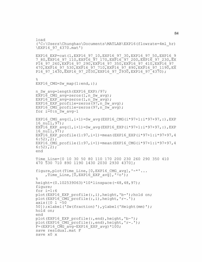
84

load ('C:\Users\Chunghao\Documents\MATLAB\EXP16(flowrate=4ml_hr)\EXP16_97_4370.mat') EXP16_EXP=cat(1,EXP16_97_10,EXP16_97_30,EXP16_97_50,EXP16_97_80,EXP16_97_110,EXP16_97_170,EXP16_97_200,EXP16_97_230,EXP16_97_260,EXP16_97_290,EXP16_97_350,EXP16_97_410,EXP16_97_470,EXP16_97_530,EXP16_97_710,EXP16_97_890,EXP16_97_1190,EXP16_97_1430,EXP16_97_2030,EXP16_97_2930,EXP16_97_4370); %

EXP16_CMG=Sw_map(1:end,:); n_Sw_avg=length(EXP16_EXP)/97; EXP16_CMG_avg=zeros(1,n_Sw_avg); EXP16_EXP_avg=zeros(1,n_Sw_avg); EXP16_EXP_profile=zeros(97,n_Sw_avg); EXP16_CMG_profile=zeros(97,n_Sw_avg); for i=0:n_Sw_avg-1 EXP16_CMG_avg(1,i+1)=Sw_avg(EXP16_CMG(i*97+1:i*97+97,:),EXP16_null,97); EXP16_EXP_avg(1,i+1)=Sw_avg(EXP16_EXP(i*97+1:i*97+97,:),EXP16_null,97); EXP16_EXP_profile(1:97,i+1)=mean(EXP16_EXP(i*97+1:i*97+97,4

6:52),2); EXP16_CMG_profile(1:97,i+1)=mean(EXP16_CMG(i*97+1:i*97+97,46:52),2); end Time_Line=[0 10 30 50 80 110 170 200 230 260 290 350 410 470 530 710 890 1190 1430 2030 2930 4370]; figure,plot(Time_Line,[0,EXP16_CMG_avg],'-*'... ,Time_Line,[0,EXP16_EXP_avg],'-o'); % height=(0.102539063)*10*linspace(-48,48,97); figure; for i=1:6

plot(EXP16_EXP_profile(:,i),height,'b-');hold on; plot(EXP16_CMG_profile(:,i),height,'r-.'); axis([0 1 -50 50]);xlabel('Sw(fraction)'),ylabel('Height(mm)'); hold on; end plot(EXP16_EXP_profile(:,end),height,'b-'); plot(EXP16_CMG_profile(:,end),height,'r-.'); F=(EXP16_CMG_avg-EXP16_EXP_avg)*100; save residual.mat F save x0 x

85

VITA

Chung-Hao Lee

Chung-Hao Lee was born in Taipei, Taiwan, in 1976. He received a bachelor's in

Resource Engineering from National Cheng Kung University, Taiwan in1999. He

pursued his graduate study in the same university and earned a Master’s degree in 2001.

Between 1999 and 2001 he also worked for Heisei Corporation as an environmental

engineer. After he graduated, he served as engineering officer, 2nd lieutenant in Matsu

Defense Command, Chinese Army. In 2003, he finished his obligatory military service

and joined Energy and Environment Research Laboratories, Industrial Technology

Research Institute, Taiwan as an associate researcher. During this period, he was actively

involved in several large-scale geological evaluation projects including spent nuclear

waste repository, geothermal, and environmental remediation. In August 2007, he started

working on his doctoral degree in Petroleum and Natural Gas Engineering at The

Pennsylvania State University. He was awarded , 2nd place in the 2010 SPE regional

student paper contest for Mid Continent/Rocky Mountain/Eastern region [PhD division].

He is special interested in multiphase flow in porous and fracture media and numerical

reservoir simulation. His research works have been published in the conference

proceedings and technical journals. He is a member of Society of Petroleum Engineers.

PARAMETRIC STUDY OF FACTORS AFFECTING CAPILLARY …

Documents

Transcript of PARAMETRIC STUDY OF FACTORS AFFECTING CAPILLARY …