PARAMETRIC ANALYSIS OF A DETONATION-TYPE TURBOFAN by ...
76
PARAMETRIC ANALYSIS OF A DETONATION-TYPE TURBOFAN by YASHWANTH M. SWAMY Presented to the Faculty of the Graduate School of The University of Texas at Arlington in Partial Fulfillment of the Requirements for the Degree of MASTER OF SCIENCE IN AEROSPACE ENGINEERING THE UNIVERSITY OF TEXAS AT ARLINGTON December 2011
Transcript of PARAMETRIC ANALYSIS OF A DETONATION-TYPE TURBOFAN by ...

PARAMETRIC ANALYSIS OF A DETONATION-TYPE TURBOFAN
by
YASHWANTH M. SWAMY
Presented to the Faculty of the Graduate School of
The University of Texas at Arlington in Partial Fulfillment
of the Requirements
for the Degree of
MASTER OF SCIENCE IN AEROSPACE ENGINEERING
THE UNIVERSITY OF TEXAS AT ARLINGTON
December 2011

Copyright © by Yashwanth M. Swamy 2011
All Rights Reserved

iii
ACKNOWLEDGEMENTS
I would like to first thank Dr. Frank Lu for his guidance throughout the project. He has
been a constant source of motivation to me and it has been a rich experience to work for him. I
would also like to thank Dr. Don Wilson and Dr. Luca Massa for taking time to serve on my
committee.
I wish to thank my parents, V M M Swamy and Naveena Swamy, who taught me every-
thing I know and supported me over the years. I would also like to thank my sister and grand-
parents for their love and support. I dedicate this thesis to my family.
November 8, 2011

iv
ABSTRACT
PARAMETRIC ANALYSIS OF A DETONATION-TYPE TURBOFAN
YASHWANTH M. SWAMY, M.S.
The University of Texas at Arlington, 2011
Supervising Professor: Dr. Frank K. Lu
A new type of turbofan which detonates a fuel-air mixture was theoretically found to perform
better than a conventional turbofan. A continuous detonation process is described and consid-
ered inside the core of the turbofan. The detonation-type turbofan needs certain modifications to
detonate the fuel-air mixture at the core of the turbofan, namely, an annular detonation chamber
to achieve continuous detonation. A parametric analysis of the new detonation-type turbofan
was developed and used to calculate the performance parameters.

v
TABLE OF CONTENTS
ACKNOWLEDGEMENTS ............................................................................................................. iii
ABSTRACT ................................................................................................................................... iv
LIST OF FIGURES ....................................................................................................................... vii
LIST OF TABLES .......................................................................................................................... ix
NOMENCLATURE ........................................................................................................................ x
Chapter Page
1. INTRODUCTION ......................................................................................................... 1
1.1 Detonation and Deflagration ............................................................................ 1
1.2 Outline .............................................................................................................. 2
1.3 Geometry and Modeling ................................................................................... 4
1.3.1 Description of Geometric Parameters ........................................... 6
1.3.2 Components of a Hybrid Turbofan ................................................ 9
1.4 Method of Analysis ......................................................................................... 12
1.5 Introduction to Isolator .................................................................................... 12
2. PARAMETRIC ANALYSIS ........................................................................................ 14
2.1 Parametric Analysis of a Normal Turbo Fan (NTF) ........................................ 14
2.1.1 Parametric Analysis of an Ordinary Turbofan ............................. 14
2.2 Parametric Analysis of Hybrid Turbo Fan (HTF) ............................................ 19
2.2.1 Temperature at station 4 ............................................................. 19
2.2.2 Modifications required: Mach number at station 4. ..................... 22
2.2.3 Flow Chart of the Complete Parametric Analysis of a HTF ........ 25
2.3 CEA [11]
(Chemical Equilibrium with Applications) .......................................... 26
3. CALCULATIONS AND RESULTS ............................................................................ 30
vi
3.1 Method of calculation ................................................................................... 30
3.2 Comparison plots ......................................................................................... 33
4. CONCLUSION AND FUTURE WORK ...................................................................... 44
4.1 Advantages of the Integrated Turbofan ........................................................ 44
4.2 Disadvantages of the Integrated Turbofan ................................................... 44
4.3 Future Work .................................................................................................. 44
APPENDIX
A. MATLAB CODE FOR HYBRID TURBOFAN ENGINE ............................................ 45
B. MATLAB CODE FOR NORMAL TURBOFAN ENGINE .......................................... 55
C. CEA INPUT AND OUTPUT ..................................................................................... 62
REFERENCES ............................................................................................................................ 64
BIOGRAPHICAL INFORMATION ............................................................................................... 65
vii
LIST OF FIGURES
Figure Page
1 Schematic of a stationary combustion wave. ..................................................................................... 1
2 Standard station numbering of a turbofan [1]
...................................................................................... 4
3 Simple front view of the detonation chamber [3]
................................................................................. 5
4 Schematic of the rotating detonation wave
structure [7]
.............................................................................................................................................. 6
5 Isometric view of the detonation chamber with
categorization [3]
.................................................................................................................................... 7
6 A conceptual sketch of a hybrid turbofan with
RDWE. .................................................................................................................................................. 10
7 A close-up view of the isolator followed by the
detonation chamber. ........................................................................................................................... 10
8 Conceptual sketch of a turbofan integrated with a RDWE. .............................................................................................................................................. 11
9 Front view of a turbofan. ..................................................................................................................... 11
10 An isometric view of the conceptual hybrid
turbofan.1.4 Method of Analysis .................................................................................................... 12
11 Rolled out view of the annular chamber denoting the parametric variable 'r'. .............................................................................................. 20
12 A typical distributions of pressure and
temperature as a function of r . ...................................................................................................... 21
13 Flow chart of the parametric analysis. ........................................................................................... 25
14 Performances of NTF and HTF versus πc,
for πf=1.2 and M0=0.7. .................................................................................................................... 33
15 Performances of NTF and HTF versus
πc, for πf=1.2 and M0=0.7. .............................................................................................................. 34
16 Comparison of performances of NTF and HTF

viii
versus πc, for πf=1.2 and M0=0.7 .................................................................................................. 35
17 Comparison of performances of NTF and HTF
versus πc, for πf=1.2 and M0=0.7 .................................................................................................. 36
18 Comparison of performances of NTF and HTF versus
πc, for πf=1.2 and M0=0.7 ............................................................................................................... 37
19 Comparison of performances of NTF and HTF versus M0 ,
for πf=1.2 and πc=1.5 ...................................................................................................................... 38
20 Comparison of performances of NTF and HTF versus M0, for
πf=1.2 and πc=1.5.Overall efficiency ........................................................................................... 39
21 Comparison of performances of NTF and HTF versus M0 ,
for πf=1.2 and πc=1.5 ...................................................................................................................... 40
22 Comparison of performances of NTF and HTF versus M0 , for πf=1.2 and πc=1.5 ...................................................................................................................... 41
23 Comparison of performances of NTF and HTF versus M0, for πf=1.2 and πc=1.5.Overall efficiency ........................................................................................... 42
ix
LIST OF TABLES
Table Page
1 Qualitative differences between
detonation and deflagration [2]
.............................................................................................................. 2
2 Detonation chamber sizing [4, 5]
............................................................................................................ 9
3 CEA output. ........................................................................................................................................... 26
4 Values of variables ahead of the TDW ( unburned gas ). .............................................................. 27
5 Values of variables behind the TDW (burned gas). ........................................................................ 27
6 Detonation parameters. ....................................................................................................................... 28
7 Base values of parameters in a NTF ................................................................................................. 31

x
NOMENCLATURE
a Size (width) of the self-excited cell of the detonation front (m/in)
u Velocity of a combustion wave
c Velocity of sound
d Mean diameter of the annular chamber
cd Diameter of the outer wall of the chamber
G Total flow rate of the mixture
g Specific flow rate of the mixture
spI Specific impulse
J Enthalpy
L Length of the chamber
l Distance between the two neighboring transverse detonation waves
M Mach number
P Pressure
Specific heat ratio
Distance between the walls of the annular chamber
Total length of the reaction zone
Total pressure ratios
Density
T Temperature
P Pressure
D Detonation wave velocity
xi
By-pass ratio
CJ Chapman-Jouguet
Subscripts
t Stagnation or total parameters
190 Station numbers of a standard turbofan
b Burner
1
CHAPTER 1
INTRODUCTION
The harnessing of detonations for aero propulsion has gained much interest in the re-
cent past. At present pulse detonation wave engines (PDWEs) and rotating or continuous deto-
nation wave engines (RDWEs or CDWEs) are being researched worldwide, for they may hold a
more efficient means of aerospace propulsion. This study is an analysis of an RDWE and
means to integrate it into a separate flow turbofan. This study also compares the performance
of the detonation-type turbofan with the performance of a standard turbofan.
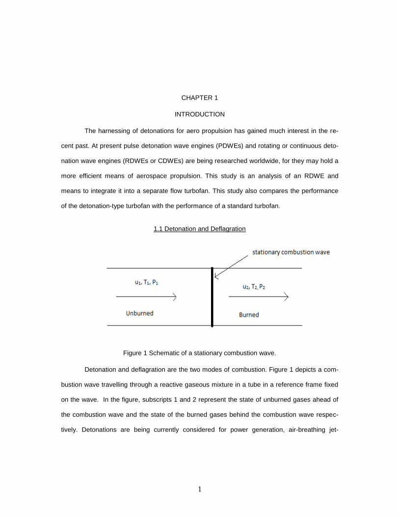
1.1 Detonation and Deflagration
Figure 1 Schematic of a stationary combustion wave.
Detonation and deflagration are the two modes of combustion. Figure 1 depicts a com-
bustion wave travelling through a reactive gaseous mixture in a tube in a reference frame fixed
on the wave. In the figure, subscripts 1 and 2 represent the state of unburned gases ahead of
the combustion wave and the state of the burned gases behind the combustion wave respec-
tively. Detonations are being currently considered for power generation, air-breathing jet-

2
engines, rockets and certain other related disciplines .Since detonation itself is preceded by a
shock wave which compresses the flow, the actual compression ratio needed by the turbo-
machinery is expected to be low in the range of 3-8. Thus, heavy turbo machinery is not ex-
pected to be required in detonation-based propulsion systems.
Table 1 Qualitative differences between detonation and deflagration [2]
Detonation Deflagration
u1/c1 5-10 0.0001-0.03
u2/u1 0.4-0.7 4-6
p2/p1 13-55(compression) ~0.98(slight expansion)
T2/T1 8-21 4-16
ρ 2/ρ1 1.7-2.6 0.006-0.25
In an ordinary turbofan, combustion of the fuel-air mixture takes place through deflagra-
tion. We will see in the present study, how detonation can be utilized instead of deflagration for
better efficiency in a turbofan. As seen in table 1, detonation waves heat the reactive gaseous
mixture to a higher temperature than its subsonic, deflagration counterpart. Detonation com-
presses flow whereas deflagration slightly expands the flow as is evident from the table. This
can be attributed to the shock wave which always precedes a detonation wave. Also seen is
that the ratio of the speed of the unburned gas to local speed of sound ( 11 cu ) is higher in the
case of detonation (due to the supersonic nature of the wave) and the ratio of the speeds of
burned to unburned gas is lower in detonation waves.
1.2 Outline
The geometry and the various constraints of the geometry of continuously rotating det-
onation wave concept in an annular chamber [3]
are described in section 1.3.The method of
analysis is described in section 1.4.

3
In the process of integration, un-starting of the engine was a primary challenge due to
the high pressures developed in the detonation chamber. There might even be a back flow of
the combustible mixture or combustion wave which is highly undesirable and potentially disas-
trous. Thus an ―Isolator‖ is integrated into the system which is expected to address this situa-
tion. Brief details about Isolator and its workings are given in section 1.5.
In CDWE, ―continuous‖ means that the detonation, which rotates around an annual
chamber, will not cease as long as reactants are fed and the combustion products are removed
continuously. Such a detonation chamber is proposed for replacing the ordinary combustion
(deflagration) chamber in a turbofan. Since a detonation wave strongly compresses the flow,
high pressures are obtained and correspondingly high temperatures, which would require exotic
alloys to withstand such extreme conditions. The exhaust enters a turbine (which provides pow-
er to the compressor and other systems) and exits into the ambient through an exhaust nozzle.
Analysis is performed to explore the performance of such an engine. More details on the analy-
sis are given in chapter 2.
Chapter 3 contains all the assumptions, methods, code descriptions, results, and dis-
cussions made.
4
1.3 Geometry and Modeling
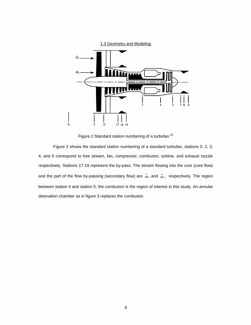
Figure 2 Standard station numbering of a turbofan [1]
Figure 2 shows the standard station numbering of a standard turbofan, stations 0, 2, 3,
4, and 5 correspond to free stream, fan, compressor, combustor, turbine, and exhaust nozzle
respectively. Stations 17-19 represent the by-pass. The stream flowing into the core (core flow)
and the part of the flow by-passing (secondary flow) are cm
and fm
respectively. The region
between station 4 and station 5, the combustor is the region of interest in this study. An annular
detonation chamber as in figure 3 replaces the combustor.

5
Figure 3 Simple front view of the detonation chamber [3]
Figure 3 is a simple visualization aid of the detonation chamber; where in an explosive
gaseous mixture of oxidizer-fuel is injected through a manifold of orifices into an annular cham-
ber of length L with being the distance between the walls of the annular chamber and with
an outer diameter cd . The governing factor in obtaining continuous detonation is the mixing in
the transverse detonation wave (TDW) front region. Another factor is the renewal of the com-
bustible/explosive mixture ahead of the TDW front. Moreover the height to which this layer is
renewed is of importance since there is a certain threshold or critical value*h , below which the
TDW will fade out. The critical value *h is related toλ , which is the total length of the reaction
zone in the detonation wave. [3]
An average relationship is provided by [3]
:
717 hh (1)

6
Figure 4 Schematic of the rotating detonation wave structure [7]
Figure 4 shows the rolled out view of the annulus where-in contact burning is shown
which has been ignored in the present study to simplify the analysis. The figure also shows a
2D view of the structure of the detonation wave and the attached oblique shock wave.
1.3.1 Description of Geometric Parameters
The value of λ is determined by the time of physical processes for formation of an ex-
plosive mixture (fragmentation of drops behind the leading shock wave, evaporation, diffusion,
and turbulent mixing of fuel components) and the subsequent time of the chemical reaction. If
an ideal case is assumed where in there is a complete pre-mixing, the characteristic chemical
length of the zone can be approximated as:
a7.0 (2)
where a is the width of the self-excited cell of the detonation front. The value of
a can be determined experimentally in detonation tubes and is known for a large number of
mixtures and can also be calculated from known methods provided the physiochemical data; [3,
9]
From (1) and (2) we obtain
ah 512 (3)
7
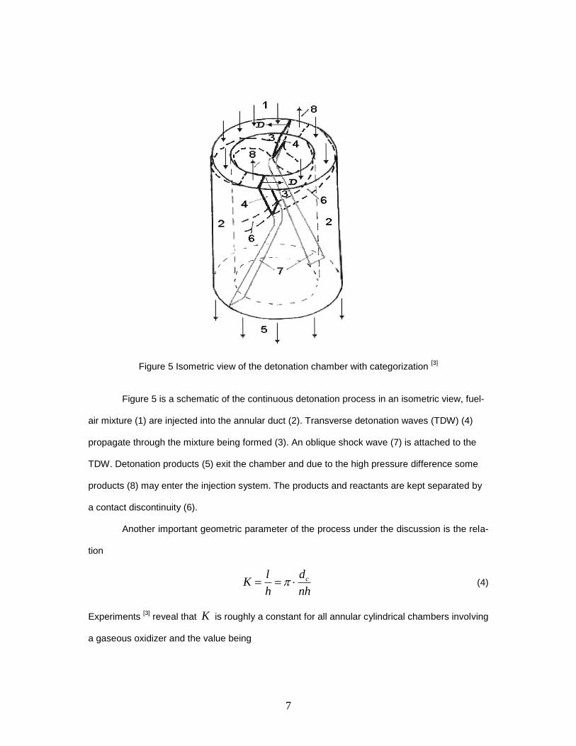
Figure 5 Isometric view of the detonation chamber with categorization [3]
Figure 5 is a schematic of the continuous detonation process in an isometric view, fuel-
air mixture (1) are injected into the annular duct (2). Transverse detonation waves (TDW) (4)
propagate through the mixture being formed (3). An oblique shock wave (7) is attached to the
TDW. Detonation products (5) exit the chamber and due to the high pressure difference some
products (8) may enter the injection system. The products and reactants are kept separated by
a contact discontinuity (6).
Another important geometric parameter of the process under the discussion is the rela-
tion
nh
d
h
lK c (4)
Experiments [3]
reveal that K is roughly a constant for all annular cylindrical chambers involving
a gaseous oxidizer and the value being
8
27K (5)
Thus, by knowing K we can back calculate the minimum chamber diameter from the previous
equation:
hKdc
min (6)
For chambers operating with a gaseous oxidizer, [3]
40min
cd (7)
The minimum length of the chambers is determined experimentally [3]
. It is approximated by the
relation
n
dhL c 2min (8)
But the continuous detonation process occurring at hL 3 is not efficient enough; it
proceeds with incomplete combustion of the fuel. The optimal length is two to three times great-
er than the minimum length
n
dlhL c
opt
27.04 (9)
The minimum possible radial size can be found from the expression
h2.0* (10)
h is determined by the critical conditions of detonation propagation; the wall friction and heat
losses of TDWs.
The data in Table 2 will facilitate the present calculations. [4]
Table 2 gives us the numer-
ical values of certain geometrical parameters which are experimentally [3, 5]
established and aid
us in calculations in section 2.2.2 and 2.2.3.

9
Table 2 Detonation chamber sizing [4, 5]
Fuel oxidizer combination ( 1 ) λ(mm) )(mh )(min md
AirH 22 10.9 0.131 0.436
The frequency of the detonation wave is given by:
mincc d
D
d
Dn
l
DF
(11)
1.3.2 Components of a Hybrid Turbofan
Most of the machinery of an ordinary turbofan is retained; both the compressor and tur-
bines are mounted on the same shaft. The number of blades on each rotor and number of stag-
es in the turbo-machinery are not considered in this study. Since a separate flow turbofan is
considered, a separate duct will be present ensuring the bypass of the secondary flow. In Fig-
ures 5---9 below, the components shown in the dark blue represents the detonation chamber
and the initial converging diverging section seen evidently in figure 7 represents a near constant
area diffuser. These figures help in visualization of the integration of detonation chamber and
isolator into a turbofan.
10
Figure 6 A conceptual sketch of a hybrid turbofan with RDWE.
Figure 7 A close-up view of the isolator followed by the detonation chamber.

11
Figure 8 Conceptual sketch of a turbofan integrated with a RDWE.
Figure 9 Front view of a turbofan.

12
Figure 10 An isometric view of the conceptual hybrid turbofan.
1.4 Method of Analysis
The turbofan with a continuous detonation engine is subjected to parametric analysis using
equations as described in chapter 2. Based on this analysis, performance parameters are de-
termined and plotted against each other following a meaningful pattern and compared to the
performance plots of a normal turbofan, collectively these plots would give us an understanding
of the overall relative engine performance.
1.5 Introduction to Isolator
Since in a detonation process, high pressures are reached in the front section of deto-
nation chamber and a low pressure area exists before the combustor, there is a possibility of a
shock wave propagating upstream which might lead to catastrophic failure. Thus, a device
called an ―isolator‖ is used, which has a unique capability of suppressing back pressure by
providing a ―shock wave cushion‖. [12]
The isolator works on the shock train concept (a series of
normal or oblique shock waves) to damp out any shock surge upstream.

13
A shock train‘s maximum pressure rise is exactly the same as that of an individual
shock wave; it is only longer and gradual, associated with boundary layer separation. For lower
supersonic entry Mach numbers usually normal shock wave trains occur and higher entry Mach
numbers oblique shock wave trains occur. Due to the effects which are only important when
there is a supersonic flight (unstart problem) or an adverse back pressure, which are isolated
cases and also due to its complexity, isolator is not considered in the present analysis.

14
CHAPTER 2
PARAMETRIC ANALYSIS
2.1 Parametric Analysis of a Normal Turbo Fan (NTF)
Parametric cycle analysis desires to determine how the engine performance (specific
thrust and fuel consumption) varies with changes in the flight conditions (e.g., Mach number),
design limits (e.g., main burner exit temperature), component performance (e.g., turbine effi-
ciency), and design choices (e.g., compressor pressure ratio).[1]
The analysis is done through a
procedure which follows energy conservation and flow balance. Since a wide range of variables
are used as parameters and their variation is studied, it is called parametric analysis, [1]
Similar
analysis is done with certain modifications at stations 3 & 4 for the HTF (hybrid turbo fan). An
open freeware called CEA was used to obtain the detonation parameters. Though these deto-
nation parameters do not affect the performance of the engine directly, the temperature and
pressure values at station 4 (combustor exit) do have a direct impact.
The following assumptions are made: [1]
1. Ideal parametric analysis is done where in the losses (aerodynamic, heat, boundary
layer, viscous, radiation etc.) are ignored and an ideal gas with constant specific heats
is considered.
2. The engine exhaust nozzles expand the gas to the ambient pressure 0PPe
2.1.1 Parametric Analysis of an Ordinary Turbofan
The following are the assumptions for the cycle analysis of a turbofan with separate exhaust
[1]
streams:
1. Perfect gas upstream of main burner with constant properties pccc cR ,, etc.
15
2. Perfect gas downstream of main burner with constant properties pttt cR ,, etc.
3. All components are adiabatic i.e. no turbine cooling.The efficiencies of the compressor,
fan and the turbine are described through the use of (constant) polytrophic efficiencies
fc ee , and te respectively.
4. The following equations[1]
are used for the analysis of a standard turbofan (for a detailed
derivation of these equations see [1]):
pc
c
c
ccR
)1( (12)
pc
t
c
tcR
)1( (13)
The local speed of sound given by
00 TRa cc (14)
To calculate velocity, provided Mach number is available:
000 MaV (15)
Static temperature and pressure ratios of the free stream are given by:
2)1(1
2
0Mcr
(16)
)1/( cc
rr
(17)
1,10 rM Since (18)
By definition
is the ratio of burner exit enthalpy to ambient enthalpy:

16
0
4
Tc
Tc
pc
tpt
(22)
The compressor pressure and temperature ratios are related by equation: [1]
cc
c
ecc
1
(23)
The compressor efficiency is given by:
1
1/)1(
c
c
c
cc
(24)
The temperature pressure ratio and the efficiency of the fan is given by equation (25) and (26)
fcc e
ff
/1
(25)
and
1
11
f
f
f
cc
(26)
A power balance of the combustor yields
0Tc
hf
pc
prb
cr
(27)
The power balance between the turbine, compressor, and fan yields
11
11
fc
n
rt
f
(28)

17
tett
tt
1
(29)
te
t
tt 1
1
1
(30)
ntbcdrt
P
P
P
P
9
0
9
9 (31)
The exit Mach number is
11
9
99
1
2
t
t
P
PM t
t
(32)
pt
pc
t
t
c
c
PPT
T
t
t
1
990
9
(33)
Expressing velocity ratios in terms of Mach numbers, temperatures, and gas properties of states
0 and 9:
0
9
9
0
9
TR
TRM
a
V
cc
tt
(34)
The ratio of total pressure of the fan to static pressure is given by:
dfnfcr
t
P
P
P
P
19
0
19
19 (35)
11
21
19
1919
cc
P
PM t
c
(36)
18
ccPPT
T
t
fr
1
19190
19
(37)
0
1919
0
19
T
TM
a
V
(38)
Combining the thrust equation for the fan stream and the engine core stream, we obtain
cc
cc
t
c
PP
aV
TTM
a
V
g
a
PP
aVR
TTRfM
a
Vf
g
a
m
F
190
019
0190
0
190
190
09
090
0
90
0
1
1
111
1
1
(39)
The thrust specific fuel consumption S is
01 mF
fS
(40)
The propulsive and thermal efficiencies are given by
2
0
2
09
2
09
0019090
11
112
MaVaVf
MaVaVMP
(41)
pr
tfh
MaVaVfa
2
11 2
0019
2
09
2
0
(42)
The overall efficiency:
Tp 0 (43)
19
2.2 Parametric Analysis of Hybrid Turbo Fan (HTF)
In a HTF, due to the addition of a detonation chamber corresponding modifications
needs to be done in the analysis procedure of a standard turbofan. Section 2.2.1 and 2.2.2 will
give more details on the modifications adapted.
2.2.1 Temperature at station 4
Section 2.1 gives us the performance of a standard turbofan without any kind of integra-
tion with new technology. HTF is integrated with a detonation chamber, therefore we need to
modify the above set of equations so that it takes into account the effect of detonation occurring
inside and reflect that in the performance. To do such an analysis of HTF, first we need to cal-
culate the detonation parameters (temperature, pressure, density, etc. changes) inside the det-
onation chamber which are sensitive to the type of fuel, initial pressure, initial temperature, and
fuel–air ratio. Thus for the sake of simplicity we shall keep most of these parameters constant
and use CEA to calculate the detonation parameters inside the detonation chamber. As we do
so, we face another problem: CEA gives the values of temperature, pressure, specific heat ra-
tio, velocity etc. directly behind the detonation wave as output, when the values of the certain
variables ahead of (combustor entry/station 3) the detonation wave are given as an input. Thus,
the values of temperature and pressure are those of points immediately behind the detonation
front and not at station 4 of the turbofan.
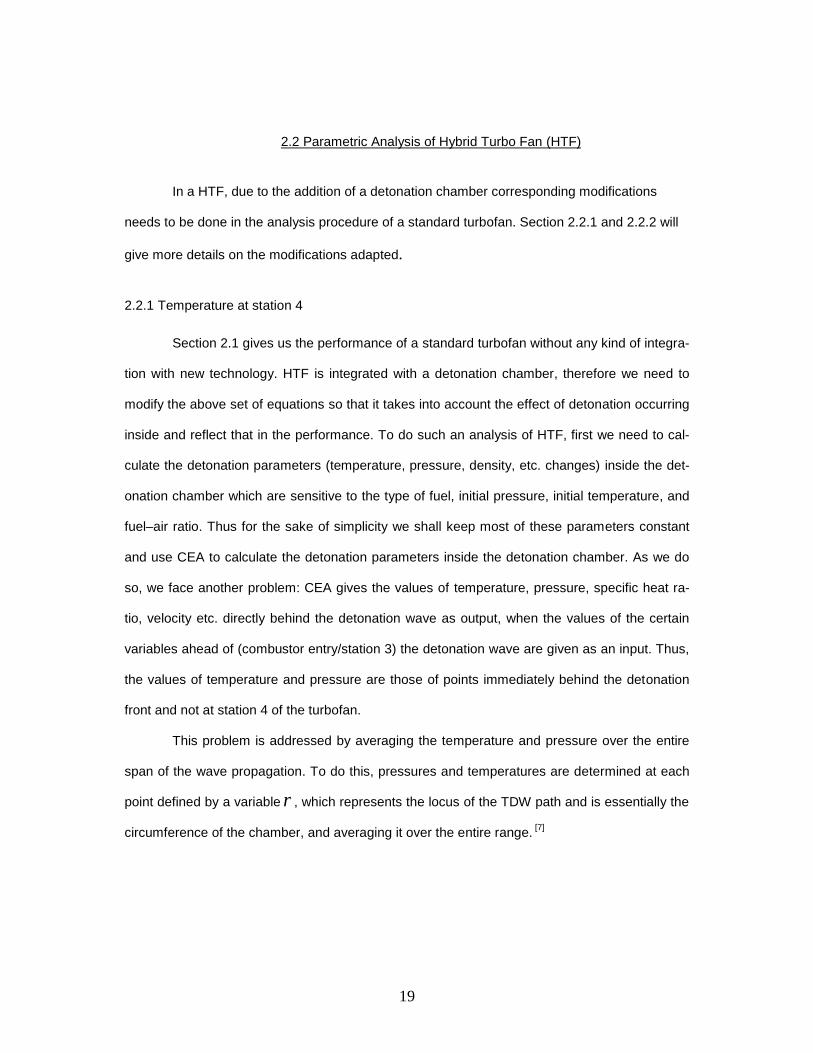
This problem is addressed by averaging the temperature and pressure over the entire
span of the wave propagation. To do this, pressures and temperatures are determined at each
point defined by a variable r , which represents the locus of the TDW path and is essentially the
circumference of the chamber, and averaging it over the entire range. [7]
20
Figure 11 Rolled out view of the annular chamber denoting the parametric variable 'r'.
The pressure and temperature at each point r are given by
[7]
cj
cj
cj
cj
rh
h
C
rCPP
cj
cj
cj
cjr
max
1
2
sin
11
(44)
cj
cj
cj
rcjr
P
PTT
1
(45)
The average of the temperature will give us the exit temperature at station 4:
r
ravg
N
TTT
4
(46)
Where rN is the total number of points at which the temperature was considered.
Similarly the pressure:
r
ravg
N
PPP
4
(47)

21
When rP is plotted against r we obtain Figure 12.
0 0.2 0.4 0.6 0.8 1 1.2 1.40
0.5
1
1.5
2x 10
6
r[m]
P(r
)[P
a]
0 0.2 0.4 0.6 0.8 1 1.2 1.4500
1000
1500
2000
2500
r[m]
T(r
)[K
]
Figure 12 A typical distributions of pressure and temperature as a function of r .
Figure 12 is a graphical representation of the temperature and pressure distribution at
each point r , obtained after solving equation (44) and (45) at each r . The equilibrium CJ point
parameters are obtained via CEA. See appendix B, code for more details.
The values of 4T and 4P can used to find the total temperatures at station 4 required in the
analysis of HTF:
2
42
442
11 MTTt
(48)

22
12
42
44
2
2
2
11
MPPt
(49)
Using Equations (48) and (49) we can evaluate:
3
4
t
tb
T
T
(50)
3
4
t
tb
P
P
(51)
2.2.2 Modifications required: Mach number at station 4.
Equation (48) and (49) still need the exit Mach number of the combustor, 4M which can
be determined by specifying values for certain geometric properties for the chosen model.
For fuel–oxidizer choice of hydrogen and air we have: [3]
0156.0a m (52)
The parameter a being the width of the self-excited cell.This parameter is easily de-
termined by known established methods and is already available for a wide range of mixtures.
For Hydrogen-air combination, (52) is determined using table 2.
The distance between neighboring detonation waves:
n
dl c
(56)
The following equation relates the total stagnation enthalpy of the mixture to the detonation
wave velocity:
112 2
2
2
0 qDJ (57)

23
Where D is the velocity of the detonation wave itself and is obtained directly from CEA.
The total stagnation enthalpy of the mixture entering the detonation chamber ‗J0‘ is then
determined using:[3]
2
1
1 22
2
0
Dq
J
(58)
The above equation is an alternative form of the Hugoniot equation expressed in terms of total
enthalpy. Further the velocity V is given by the equation [3]
:
1
12 0
JV (59)
To incorporate a part of mass flux that comes into the detonation wave under study
from the previous detonation wave which has just preceded, a factor called k is introduced; for
our current study. We will assume a value,
15.0k (60)
The values of 2,p,2122 Tc,γ,γ,a,q are obtained from CEA software which determines
Chapman-Jouguet wave parameters.
Total mixture flow rate for a single wave, specific mixture flow rate, density, pressure and Mach
number are given by following equations:
221221 1 qhqhkG (61)
2
1
ms
Kg
l
Gg
(62)
3m
Kg
V
g (63)
24
2
gVP (64)
2
4a
VM (65)
So now we have all the inputs required for the parametric analysis of the HTF, with
equations similar to those used for the analysis of a standard turbofan (energy and flow balance
equations). Once the new values of b
and b
are substituted for the previous ones, various
performance parameters can thus be determined and compared with that of a NTF.
25
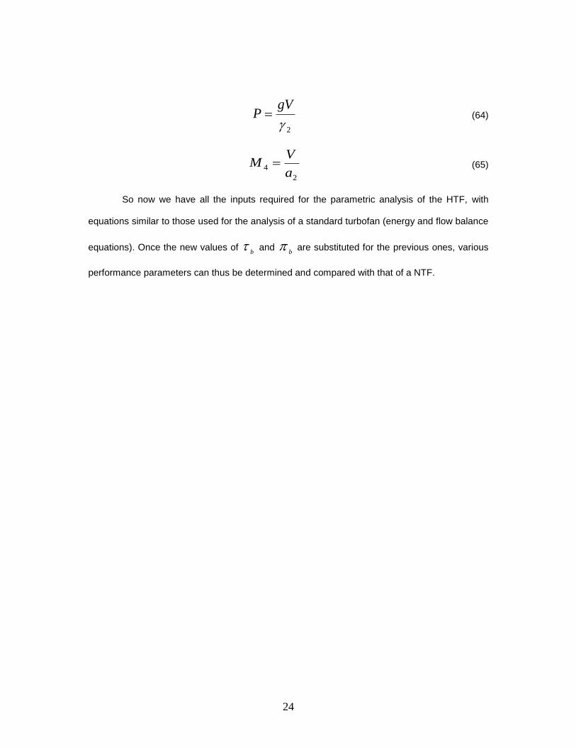
2.2.3 Flow Chart of the Complete Parametric Analysis of a HTF
Figure 13 Flow chart of the parametric analysis .
hda c ,,, (Geometrical
parameters [3]
)
rPT cjcjcj ,,,
Fuel-oxidizer combina-tion, initial pressure and
temperature, and (use
CEA)
0, ,,, JDcq p
(CEA output)
4, M
Annular chamber
model [3]
44 , PT
Annular detonation wave properties [3,4,5,7]
44 , tt PT .
Compressible flow equa-tions
[5]
New bb ,
Parametric Analysis using Ener-gy and flow Balance methods.

26
2.3 CEA [11]
(Chemical Equilibrium with Applications)
The NASA program CEA calculates chemical equilibrium compositions and properties
of a wide range of fuel-oxidizer mixtures. Applications include assigned thermodynamic states,
theoretical rocket performance, Chapman-Jouguet detonations, and shock-tube parameters for
incident and reflected shocks. CEA represents the latest in a number of computer programs that
have been developed at the NASA Lewis (now Glenn) Research Center during the last 45
years. [11]
Over 2000 species are contained in the thermodynamic database. The program is
written in ANSI standard FORTRAN by Bonnie J. McBride and Sanford Gordon. [11]
Inputs required for Chapman-Jouguet detonation process:
Chemical equivalence ratio: ( ): this ratio indicates the ratio of fuel to oxidizer. A ratio
of one ensures maximum combustion.
Fuel-oxidizer choice: Out of the 2000-odd chemical species available an appropriate
detonation mixture needs to be selected.
Initial temperature and pressure
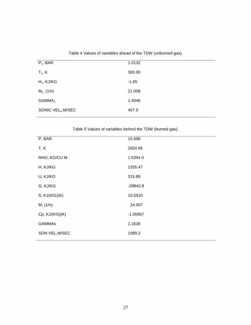
An example of a CEA output is partially shown in Tables 3-6 below:
Detonation properties of an ideal reacting gas
Case = Air-hydrogen
Table 3 CEA output.
REACTANT WT FRACTION Energy (KJ/KG-Mole) T (K )
Fuel H2 1.0000000 53.359 300.000
Oxidant Air 1.0000000 -71.689 300.000
O/F= 1.00000 %FUEL= 50.000000 R, EQ.RATIO=34.245598 PHI, EQ.RATIO=34.296226
27
Table 4 Values of variables ahead of the TDW (unburned gas).
P1, BAR 1.0132
T1, K 300.00
H1, KJ/KG -1.65
M1, (1/n) 21.008
GAMMA1 1.4046
SONIC VEL1,M/SEC 407.9
Table 5 Values of variables behind the TDW (burned gas).
P, BAR 15.696
T, K 2934.85
RHO, KG/CU M 1.5394 0
H, KJ/KG 1335.47
U, KJ/KG 315.89
G, KJ/KG -29842.8
S, KJ/(KG)(K) 10.5910
M, (1/n) 24.007
Cp, KJ/(KG)(K) -1.00957
GAMMAs 1.1636
SON VEL,M/SEC 1089.2

28
Table 6 Detonation parameters.
P/P1 15.491
T/T1 9.813
M/M1 1.1427
RHO/RHO1 1.8039
DET MACH NUMBER 4.8169
DET VEL, M/SEC 1964.9
Table 3 indicates which combination of fuel-oxidizer mixture are being used, their tem-
perature, heat of formation, and relative weight fractions. Table 4 contains more information
about the explosive mixture which is directly ahead of the TDW (unburned gas) which includes
pressure, temperature, ratio of specific heats, local speed of sound, specific heat of the mixture,
and the molecular weight of the mixture. Apart from these, table 5 and table 6 list the values of
several other variables/parameters of detonation of which density, molar standard state enthal-
py, local speed of sound behind the TDW, ratio of specific heats, specific heat, detonation Mach
number, and detonation velocity are the ones we use in our calculation.
In this chapter we saw how the parametric analysis of a standard turbofan is modified to
fit a detonation-type turbofan. In chapter 3 we will see the actual methods for calculations, as-
sumptions made, code descriptions and results obtained.
As the flight condition changes, input conditions to the burner change as well. To account for
those changes, input temperature and pressure to the burner are calculated using the following
compressible flow equations.

29
12
3
12
00
3
2
11
2
11
M
MP
P
fc
(66)
2
3
2
00
3
2
11
2
11
M
MT
T
fc
(67)
The data obtained from the equations (66) and (67) are given in the appendix C

30
CHAPTER 3
CALCULATIONS AND RESULTS
3.1 Method of calculation
Calculations for a HTF is done by coupling the data from CEA, Table 3--6 to the Matlab
code, and executing the code given in appendix A. The output is a huge array of numbers,
which were tabulated and plotted. Partial validation of these codes was done by comparing the
results with a standard text book problem and its solution; they were in excellent agreement.
The equations were programmed in Matlab. Appendix A is the Matlab code for the HTF
and appendix B is the Matlab code for the standard turbofan. The code in appendix A has sev-
eral bits to it; it begins with vectorizing the input variables. Following which there are bits of code
which calculate the exit Mach number, exit temperature and pressure at station 4, in turn deter-
mining the new b and b . Then the next part of the code substitutes the new values of b
and b for the old ones and the parametric analysis procedure is followed as in chapter 2 to
find the performance parameters. See appendix A for more details.
The calculations presented here include certain assumptions as listed below:
1. U.S standard pressure and atmosphere values are used.
2. For simplicity M3= 0.5.
3. Value of 15.0k , equation (60).
4. Subsonic flight.

31
A detailed procedure of obtaining the below plots is as follows:
Table 7 Base values of parameters in a NTF
M0=0.7 T0=390o R
γc=1.4 Cpc=0.240 Btu/lbm.oR
γt=1.33 Cpt=0.276 Btu/lbm.oR
hpr=18400 Btu/lbm πdmax=0.99
πb=0.96 πn=0.99
πfn=0.99 ec=0.90
ef=0.89 et=0.89
ηb=0.99 ηn=0.99
P0/P9=0.99 P0/P19=0.99
Tt4=3000oR
πc=3
πf=1.2 α=0.5
Table 7 shows all the parameters and their base values used in the calculation of the
performance parameters; polytrophic efficiencies nb , are kept constant to simplify the calcu-
lations. Burnt gas (core flow) and the secondary flow are assumed to expand to ambient pres-
sure thus ,90 PP and 190 PP are very close to unity. The only parameters which will be varied
are ,,,0 fcM and . Also, prh is a parameter which is a constant for a specific fuel. The
rest of the parameters are assumed constant throughout the calculations.
For a HTF b and 4tT are calculated from the values obtained from CEA and the
method described in chapter 2, then substituted for the old values and the performance analysis
is done using the code in Appendix A.
32
In figures 13—22 certain performance parameters are plotted and compared, definitions
of these parameters are given below: [1]
1. Specific thrust (
mF / ): It is defined as the ratio of net thrust to the rate of total airflow intake.
2. Thrust specific fuel consumption ( S ): It is the rate of fuel used by the propulsion system per
unit rate of thrust produced.
3. Propulsive efficiency ( p ): It is a degree of how effectively the engine power is used to power
the aircraft. It is also the ratio of aircraft power (thrust times velocity) to the power output of the
engine.
4. Thermal efficiency ( T ): It is the net rate of organized energy (shaft power or kinetic energy)
out of the engine to the rate of thermal energy available from the fuel-air mixture.
5. Overall efficiency ( 0 ): It is the ratio of aircraft power to the ratio of thermal energy released.
It equals the product of propulsive efficiency and thermal efficiency
For figure 13—17 the following flight conditions and design inputs were used:
7.00 M ,oT 3900 R,
o
tT 30004 R (only for a standard turbofan), and 2.1f .
For figure 18—22 the following flight conditions were used:
5.1c ,oT 3900 R,
o
tT 30004 R (only for a standard turbofan), and 2.1f .

33
3.2 Comparison plots The following graphs are obtained.
Figure 14 Performances of NTF and HTF versus πc, for πf=1.2 and M0=0.7.

34
Figure 15 Performances of NTF and HTF versus πc, for πf=1.2 and M0=0.7.

35
Figure 16 Comparison of performances of NTF and HTF versus πc, for πf=1.2 and M0=0.7

36
Figure 17 Comparison of performances of NTF and HTF versus πc, for πf=1.2 and M0=0.7
37
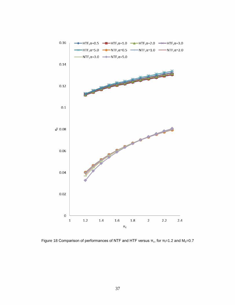
Figure 18 Comparison of performances of NTF and HTF versus πc, for πf=1.2 and M0=0.7

38
Figure 19 Comparison of performances of NTF and HTF versus M0, for πf=1.2 and πc=1.5

39
Figure 20 Comparison of performances of NTF and HTF versus M0, for πf = 1.2 and πc = 1.5

40
Figure 21 Comparison of performances of NTF and HTF versus M0, for πf=1.2 and πc=1.5
41
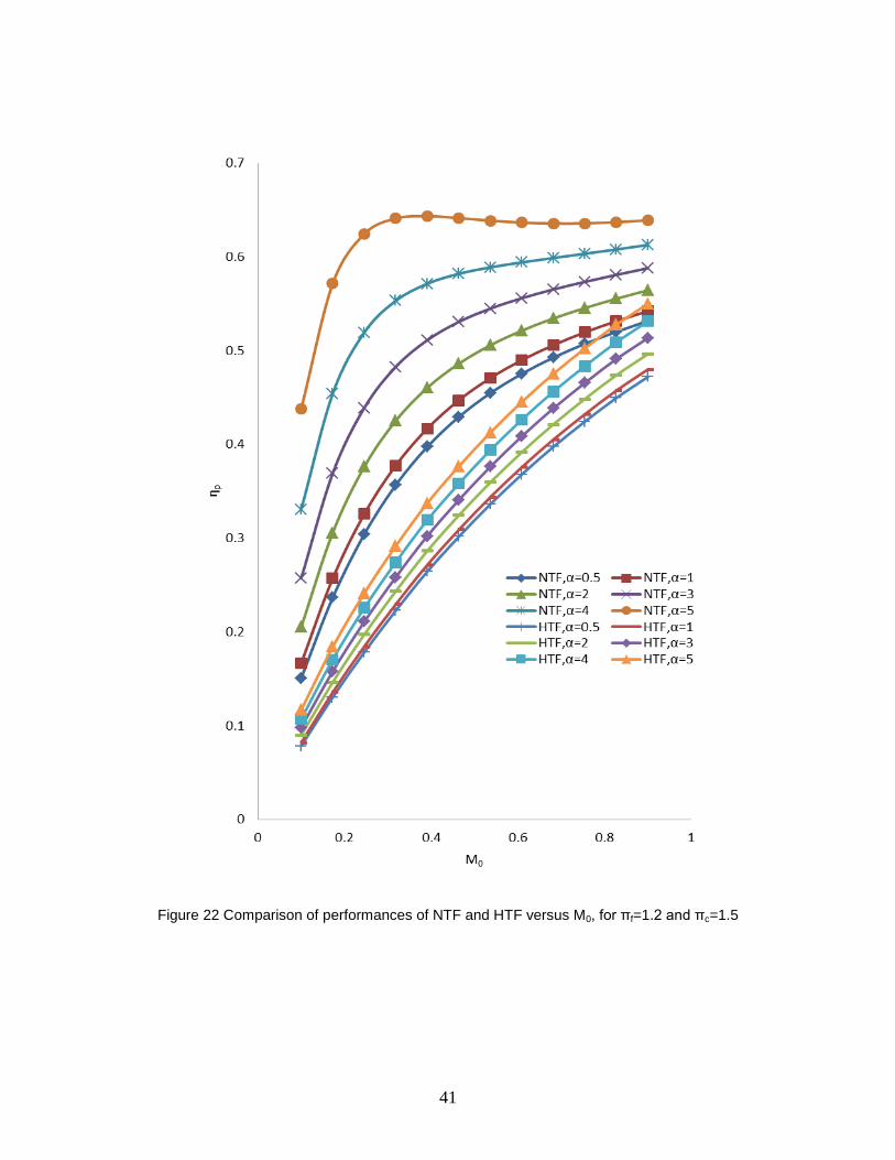
Figure 22 Comparison of performances of NTF and HTF versus M0, for πf=1.2 and πc=1.5

42
Figure 23 Comparison of performances of NTF and HTF versus M0, for πf=1.2 and πc=1.5.Overall efficiency
43
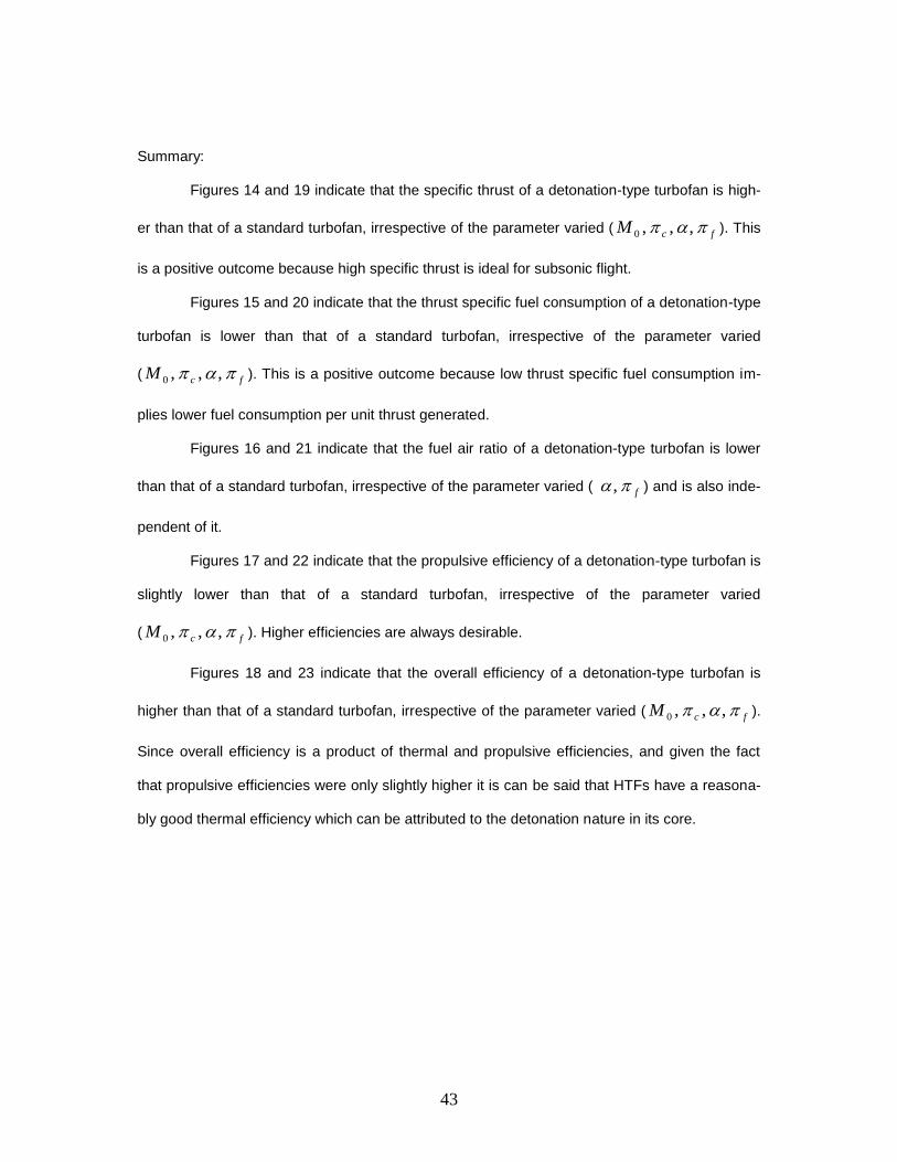
Summary:
Figures 14 and 19 indicate that the specific thrust of a detonation-type turbofan is high-
er than that of a standard turbofan, irrespective of the parameter varied ( fcM ,,,0 ). This
is a positive outcome because high specific thrust is ideal for subsonic flight.
Figures 15 and 20 indicate that the thrust specific fuel consumption of a detonation-type
turbofan is lower than that of a standard turbofan, irrespective of the parameter varied
( fcM ,,,0 ). This is a positive outcome because low thrust specific fuel consumption im-
plies lower fuel consumption per unit thrust generated.
Figures 16 and 21 indicate that the fuel air ratio of a detonation-type turbofan is lower
than that of a standard turbofan, irrespective of the parameter varied ( f , ) and is also inde-
pendent of it.
Figures 17 and 22 indicate that the propulsive efficiency of a detonation-type turbofan is
slightly lower than that of a standard turbofan, irrespective of the parameter varied
( fcM ,,,0 ). Higher efficiencies are always desirable.
Figures 18 and 23 indicate that the overall efficiency of a detonation-type turbofan is
higher than that of a standard turbofan, irrespective of the parameter varied ( fcM ,,,0 ).
Since overall efficiency is a product of thermal and propulsive efficiencies, and given the fact
that propulsive efficiencies were only slightly higher it is can be said that HTFs have a reasona-
bly good thermal efficiency which can be attributed to the detonation nature in its core.

44
CHAPTER 4
CONCLUSION AND FUTURE WORK
4.1 Advantages of the Integrated Turbofan
The Matlab code written is versatile and can be modified to analyze different types of air-
breathing engines. The actual detonation-based TF has an improved performance over the
conventional TF as shown in the results. This is attributed to the detonation process having a
better thermal efficiency.
4.2 Disadvantages of the Integrated Turbofan
There can be a safety issue since we are dealing with detonations and very high pressure
ratios. Thus further considerations are required compared to a standard turbofan. Since ex-
tremely high temperatures are produced inside the detonation chamber more new exotic alloys
are required to withstand such temperatures which might not yet be available on a commercial
scale.
4.3 Future Work
A more detailed performance analysis of the integrated TF will be done along with nu-
merical simulation of the shock wave train inside of the constant area duct (isolator) and also of
the detonation wave inside the detonation chamber. This will lead us to a better understanding
of the practicality of detonations in real aircraft engines. Also more parameters will be included
in the analysis and an off-design point performance analysis will be done in which more varia-
tion in the input parameters of the detonation chamber will be considered.

45
APPENDIX A
MATLAB CODE FOR HYBRID TURBOFAN ENGINE

46
function [F_mo,f,S,muuT,muuP,Muu0,muuC,Muut]=CDE_integrated_Turbofan (M0,T0,gammac,Cpc,gammat,Cpt,Hpr,pidmax,pib,pin,pifn,ec,ef,et,muub,muun,P0_P9,P0_P19,Tt4,pic,pif,alpha); %% % % sample syntax: % % Turbofan ([1,2,3,4],2,3,4,5,6,7,8,9,1,2,4,5,3,6,7,8,9,1,2,3,4,5) % % CDE_integrated_Turbofan (M0,T0,gammac,Cpc,gammat,Cpt,Hpr,pidmax,pib,pin,pifn,ec,ef,et,muub,muun,P0_P9,P0_P19,Tt4,pic,pif,alpha) % % CDE_integrated_Turbofan (.7,390,1.4,0.240,1.33,0.276,18400,0.99,0.96,0.99,0.99,0.90,0.89,0.89,0.99,0.99,0.9,0.9,3000,3:.4167:8,2,.5) clc; clear taub disp('Please enter the values of the input arguments as arrays of equal lengths.') %%Air & H2%%%%%%%%% %% subscript 1 & 2 coresponds to the parameters before and after the TDW %% respectively %% Vectorizing Y=ones(1,12); if size(M0)<=1 M0=M0*Y else M0=M0 end if size(T0)<=1 T0=T0*Y; else T0=T0 end if size(gammac)<=1 gammac=gammac*Y; else gammac=gammac end if size(Cpc)<=1 Cpc=Cpc*Y; else Cpc=Cpc end if size(gammat)<=1 gammat=gammat*Y; else gammat=gammat end

47
if size(Cpt)<=1 Cpt=Cpt*Y; else Cpt=Cpt end if size(Hpr)<=1 Hpr=Hpr*Y; else Hpr=Hpr end if size(pidmax)<=1 pidmax=pidmax*Y; else pidmax=pidmax end if size(pin)<=1 pin=pin*Y; else pin=pin end if size(pifn)<=1 pifn=pifn*Y; else pifn=pifn end if size(ec)<=1 ec=ec*Y; else ec=ec end if size(ef)<=1 ef=ef*Y; else ef=ef end if size(et)<=1 et=et*Y; else et=et end if size(muub)<=1 muub=muub*Y; else muub=muub end if size(muun)<=1 muun=muun*Y; else muun=muun end
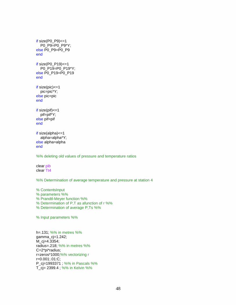
48
if size(P0_P9)<=1 P0_P9=P0_P9*Y; else P0_P9=P0_P9 end if size(P0_P19)<=1 P0_P19=P0_P19*Y; else P0_P19=P0_P19 end if size(pic)<=1 pic=pic*Y; else pic=pic end if size(pif)<=1 pif=pif*Y; else pif=pif end if size(alpha)<=1 alpha=alpha*Y; else alpha=alpha end %% deleting old values of pressure and temperature ratios clear pib clear Tt4 %% Determination of average temperature and pressure at station 4 % ContentsInput % parameters %% % Prandtl-Meyer function %% % Determination of P,T as afunction of r %% % Determination of average P,Ts %% % Input parameters %% h=.131; %% in metres %% gamma_cj=1.242; M_cj=4.3354; radius=.218; %% in metres %% C=2*pi*radius; r=zeros*1000;%% vectorizing r r=0.001:.01:C; P_cj=1993371 ; %% in Pascals %% T_cj= 2399.4 ; %% in Kelvin %%
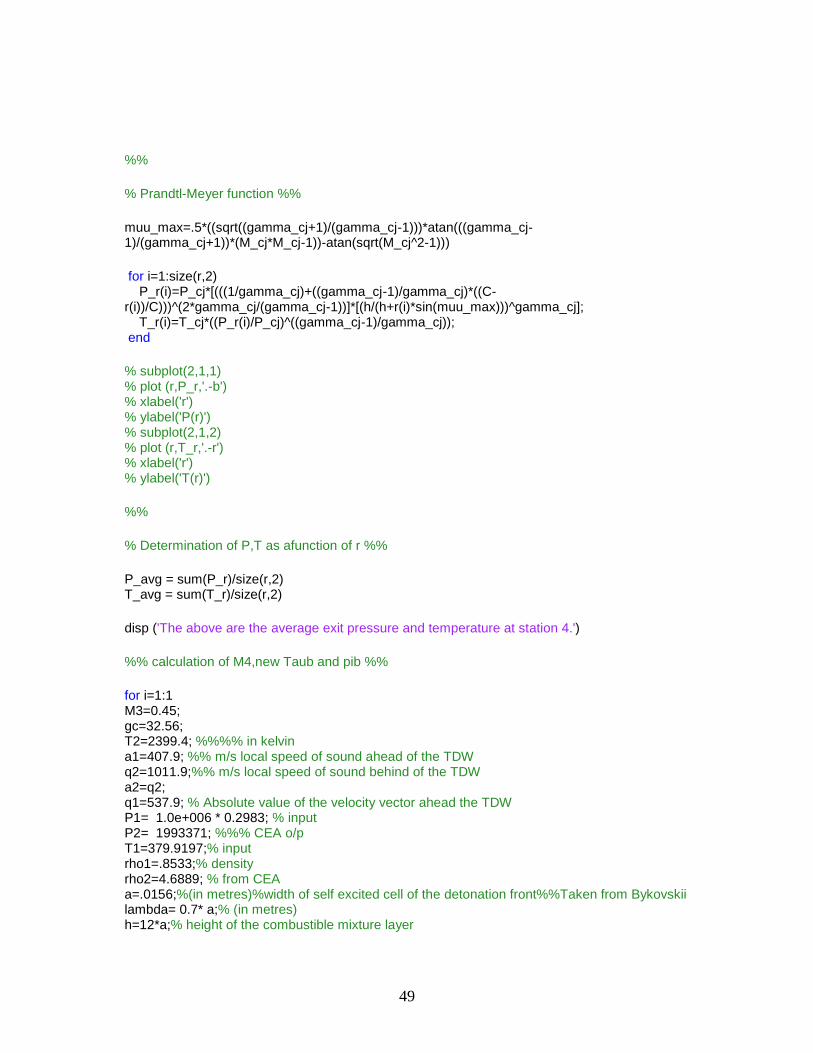
49
%% % Prandtl-Meyer function %% muu_max=.5*((sqrt((gamma_cj+1)/(gamma_cj-1)))*atan(((gamma_cj-1)/(gamma_cj+1))*(M_cj*M_cj-1))-atan(sqrt(M_cj^2-1))) for i=1:size(r,2) P_r(i)=P_cj*[(((1/gamma_cj)+((gamma_cj-1)/gamma_cj)*((C-r(i))/C)))^(2*gamma_cj/(gamma_cj-1))]*[(h/(h+r(i)*sin(muu_max)))^gamma_cj]; T_r(i)=T_cj*((P_r(i)/P_cj)^((gamma_cj-1)/gamma_cj)); end % subplot(2,1,1) % plot (r,P_r,'.-b') % xlabel('r') % ylabel('P(r)') % subplot(2,1,2) % plot (r,T_r,'.-r') % xlabel('r') % ylabel('T(r)') %% % Determination of P,T as afunction of r %% P_avg = sum(P_r)/size(r,2) T_avg = sum(T_r)/size(r,2) disp ('The above are the average exit pressure and temperature at station 4.') %% calculation of M4,new Taub and pib %% for i=1:1 M3=0.45; gc=32.56; T2=2399.4; %%%% in kelvin a1=407.9; %% m/s local speed of sound ahead of the TDW q2=1011.9;%% m/s local speed of sound behind of the TDW a2=q2; q1=537.9; % Absolute value of the velocity vector ahead the TDW P1= 1.0e+006 * 0.2983; % input P2= 1993371; %%% CEA o/p T1=379.9197;% input rho1=.8533;% density rho2=4.6889; % from CEA a=.0156;%(in metres)%width of self excited cell of the detonation front%%Taken from Bykovskii lambda= 0.7* a;% (in metres) h=12*a;% height of the combustible mixture layer
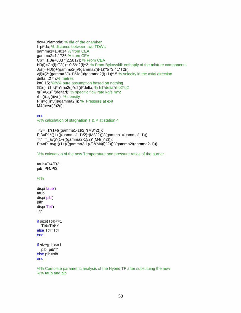
50
dc=40*lambda; % dia of the chamber l=pi*dc; % distance between two TDWs gamma1=1.4014;% from CEA gamma2=1.1736;% from CEA Cp= 1.0e+003 *[2.5817]; % From CEA H0(i)=Cp(i)*T2(i)+ 0.5*q2(i)^2; % From Bykovskii: enthaply of the mixture components Jo(i)=H0(i)+(gamma2(i)/(gamma2(i)-1))*573.41*T2(i); v(i)=(2*(gamma2(i)-1)*Jo(i)/(gamma2(i)+1))^.5;% velocity in the axial direction delta=.2 *h;% metres k=0.15; %%% pure assumption based on nothing. G1(i)=(1-k)*h*rho2(i)*q2(i)*delta; % h1*delta*rho2*q2 g(i)=G1(i)/(delta*l); % specific flow rate kg/s.m^2 rho(i)=g(i)/v(i); % density P(i)=g(i)*v(i)/gamma2(i); % Pressure at exit M4(i)=v(i)/a2(i); end %% calculation of stagnation T & P at station 4 Tt3=T1*(1+(((gamma1-1)/2)*(M3^2))); Pt3=P1*((1+(((gamma1-1)/2)*(M3^2)))^(gamma1/(gamma1-1))); Tt4=T_avg*(1+(((gamma2-1)/2)*(M4(i)^2))); Pt4=P_avg*((1+(((gamma2-1)/2)*(M4(i)^2)))^(gamma2/(gamma2-1))); %% calcuation of the new Temperature and pressure ratios of the burner taub=Tt4/Tt3; pib=Pt4/Pt3; %% disp('taub') taub' disp('pib') pib' disp('Tt4') Tt4' if size(Tt4)<=1 Tt4=Tt4*Y else Tt4=Tt4 end if size(pib)<=1 pib=pib*Y else pib=pib end %% Complete parametric analysis of the Hybrid TF after substituing the new %% taub and pib

51
%%%%%%%%%%%%%%%% JDMs nest%%%%%%%%%%%%%%%%%%% for i=1:12 Rc(i)=(gammac(i)-1)*Cpc(i)*778.16/gammac(i); Rt(i)=(gammat(i)-1)*Cpt(i)*778.16/gammat(i); a0(i)=sqrt(gammac(i)*Rc(i)*gc*T0(i)); taur(i)=1+(gammac(i)-1)*M0(i)*M0(i)/2; pir(i)=taur(i)^(gammac(i)/(gammac(i)-1)); if M0(i)<=1; muur(i)=1; else muur(i)=1-.0075*((M0(i)-1)^1.35); end pid(i)=pidmax(i)*muur(i); taulambda(i)=(Cpt(i)*Tt4(i))/(Cpc(i)*T0(i)); tauc(i)=(pic(i))^((gammac(i)-1)/(gammac(i)*ec(i))); muuc(i)=(pic(i)^((gammac(i)-1)/gammac(i))-1)/(tauc(i)-1); tauf(i)=pif(i)^((gammac(i)-1)/(gammac(i)*ef(i))); muuf(i)=((pif(i)^((gammac(i)-1)/(gammac(i))))-1)/(tauf(i)-1); f(i)=(taulambda(i)-(taur(i)*tauc(i)))/(((muub(i)*Hpr(i))/(Cpc(i)*T0(i)))-taulambda(i)); taut(i)=1-((taur(i)/(muun(i)*(1+f(i))*taulambda(i)))*(tauc(i)-1+alpha(i)*(tauf(i)-1))); pit(i)=(taut(i))^(gammat(i)/((gammat(i)-1)*et(i))); muut(i)=(1-taut(i))/(1-taut(i)^(1/et(i))); Pt9_P9(i)=(P0_P9(i))*pir(i)*pid(i)*pic(i)*pib(i)*pit(i)*pin(i); M9(i)=sqrt((2/(gammat(i)-1))*(((Pt9_P9(i))^((gammat(i)-1)/gammat(i)))-1));

52
T9_T0(i)=(taulambda(i)*taut(i)*Cpc(i))/(((Pt9_P9(i))^((gammat(i)-1)/gammat(i)))*Cpt(i)); V9_a0(i)=M9(i)*sqrt((gammat(i)*Rt(i))/(gammac(i)*Rc(i))*(T9_T0(i))); Pt19_P19(i)=(P0_P19(i))*pir(i)*pid(i)*pif(i)*pifn(i); M19(i)=sqrt((2/(gammac(i)-1))*(((Pt19_P19(i))^((gammac(i)-1)/gammac(i)))-1)); T19_T0(i)=(taur(i)*tauf(i))/((Pt19_P19(i))^((gammac(i)-1)/gammac(i))); V19_a0(i)=M19(i)*(T19_T0(i))^.5; F_mo(i)=[(1/(1+alpha(i)))*(a0(i)/gc)*(((1+f(i))*V9_a0(i))-M0(i)+((1+f(i))*((Rt(i)*T9_T0(i))/(Rc(i)*V9_a0(i)))*((1-P0_P9(i))/gammac(i))))]+[(alpha(i)/(1+alpha(i)))*(a0(i)/gc)*(V19_a0(i)-M0(i)+((T19_T0(i))/(V19_a0(i))*((1-P0_P19(i))/gammac(i))))]; S(i)=f(i)*3600/((1+alpha(i))*F_mo(i)); MuuP(i)=((2*M0(i)*(((1+f(i))*V9_a0(i))+(alpha(i)*V19_a0(i))-(1+alpha(i))*M0(i))))/((1+f(i))*(V9_a0(i)^2)+(alpha(i)*(V19_a0(i))^2)-((1+alpha(i))*(M0(i)^2))); MuuT(i)=(a0(i)^2)*((1+f(i))*(V9_a0(i))^2+alpha(i)*(V19_a0(i)^2)-(1+alpha(i))*M0(i)^2)/(2*gc*f(i)*Hpr(i)*778.16); MuuO(i)=MuuP(i)*MuuT(i); end %% Displaying output disp('pid') pid' disp('taulambda') taulambda' disp('tauc') tauc' disp('muuc') muuc' disp('tauf') tauf' disp('taut') taut' disp('pit') pit' disp('muut') muut' disp('Pt9_P9') Pt9_P9' disp('M9')
53
M9' disp('T9_T0') T9_T0' disp('V9_a0') V9_a0' disp('Pt19_P19') Pt19_P19' disp('M19') M19' disp('T19_T0') T19_T0' disp('V19_a0') V19_a0' disp('F_mo') F_mo' disp('S') S' disp('f') f' disp('MuuP') MuuP' disp('MuuO') MuuO' %% Plotting output % figure,plot (pic,F_mo) % xlabel('pic') % ylabel('F_mo') % figure,plot (pic,S) % xlabel('pic') % ylabel('S') % % figure,plot (pic,MuuP) % % xlabel('pic') % % ylabel('muup') % % figure,plot (pic,MuuO) % % xlabel('pic') % % ylabel('muuO') % % figure,plot (pif,F_mo) % xlabel('pif') % ylabel('F_mo') % figure,plot (pif,S) % xlabel('pif') % ylabel('S') % % figure,plot (pif,MuuO) % % xlabel('pif') % % ylabel('muuO') % % figure,plot (pif,MuuP) % % xlabel('pif') % % ylabel('muup')

54
% % figure,plot (M0,F_mo) % xlabel('M0') % ylabel('F_mo') % figure,plot (M0,S) % xlabel('M0') % ylabel('S') % figure,plot (M0,MuuP) % xlabel('M0') % ylabel('muup') % figure,plot (M0,MuuO) % xlabel('M0') % ylabel('muuO')

55
APPENDIX B
MATLAB CODE FOR NORMAL TURBOFAN ENGINE

56
function [F_mo,f,S,muuT,muuP,Muu0,muuC,Muut]=Turbofan_Normal (M0,T0,gammac,Cpc,gammat,Cpt,Hpr,pidmax,pib,pin,pifn,ec,ef,et,muub,muun,P0_P9,P0_P19,Tt4,pic,pif,alpha); %% % % sample syntax: % % Turbofan_Normal ([1,2,3,4],2,3,4,5,6,7,8,9,1,2,4,5,3,6,7,8,9,1,2,3,4,5) % % Turbofan_Normal (M0,T0,gammac,Cpc,gammat,Cpt,Hpr,pidmax,pib,pin,pifn,ec,ef,et,muub,muun,P0_P9,P0_P19,Tt4,pic,pif,alpha) % % Turbofan_Normal (.7,390,1.4,0.240,1.33,0.276,18400,0.99,0.96,0.99,0.99,0.90,0.89,0.89,0.99,0.99,0.9,0.9,3000,3:.4167:8,2,.5) clc; disp('Please enter the values of the input arguments as arrays of equal lengths.') %%Air & H2%%%%%%%%% %% subscript 1 & 2 coresponds to the parameters before and after the TDW %% respectively %% Vectorizing Y=ones(1,12); if size(M0)<=1 M0=M0*Y else M0=M0 end if size(T0)<=1 T0=T0*Y; else T0=T0 end if size(gammac)<=1 gammac=gammac*Y; else gammac=gammac end if size(Cpc)<=1 Cpc=Cpc*Y; else Cpc=Cpc end if size(gammat)<=1 gammat=gammat*Y; else gammat=gammat end if size(Cpt)<=1

57
Cpt=Cpt*Y; else Cpt=Cpt end if size(Hpr)<=1 Hpr=Hpr*Y; else Hpr=Hpr end if size(pidmax)<=1 pidmax=pidmax*Y; else pidmax=pidmax end if size(pin)<=1 pin=pin*Y; else pin=pin end if size(pifn)<=1 pifn=pifn*Y; else pifn=pifn end if size(ec)<=1 ec=ec*Y; else ec=ec end if size(ef)<=1 ef=ef*Y; else ef=ef end if size(et)<=1 et=et*Y; else et=et end if size(muub)<=1 muub=muub*Y; else muub=muub end if size(muun)<=1 muun=muun*Y; else muun=muun end if size(P0_P9)<=1
58
P0_P9=P0_P9*Y; else P0_P9=P0_P9 end if size(P0_P19)<=1 P0_P19=P0_P19*Y; else P0_P19=P0_P19 end if size(pic)<=1 pic=pic*Y; else pic=pic end if size(pif)<=1 pif=pif*Y; else pif=pif end if size(alpha)<=1 alpha=alpha*Y; else alpha=alpha end if size(Tt4)<=1 Tt4=Tt4*Y else Tt4=Tt4 end if size(pib)<=1 pib=pib*Y else pib=pib end gc=32.56; %% Complete parametric analysis of the normal TF %%%%%%%%%%%%%%%% JDMs nest%%%%%%%%%%%%%%%%%%% for i=1:12 Rc(i)=(gammac(i)-1)*Cpc(i)*778.16/gammac(i); Rt(i)=(gammat(i)-1)*Cpt(i)*778.16/gammat(i); a0(i)=sqrt(gammac(i)*Rc(i)*gc*T0(i)); taur(i)=1+(gammac(i)-1)*M0(i)*M0(i)/2;

59
pir(i)=taur(i)^(gammac(i)/(gammac(i)-1)); if M0(i)<=1; muur(i)=1; else muur(i)=1-.0075*((M0(i)-1)^1.35); end pid(i)=pidmax(i)*muur(i); taulambda(i)=(Cpt(i)*Tt4(i))/(Cpc(i)*T0(i)); tauc(i)=(pic(i))^((gammac(i)-1)/(gammac(i)*ec(i))); muuc(i)=(pic(i)^((gammac(i)-1)/gammac(i))-1)/(tauc(i)-1); tauf(i)=pif(i)^((gammac(i)-1)/(gammac(i)*ef(i))); muuf(i)=((pif(i)^((gammac(i)-1)/(gammac(i))))-1)/(tauf(i)-1); f(i)=(taulambda(i)-(taur(i)*tauc(i)))/(((muub(i)*Hpr(i))/(Cpc(i)*T0(i)))-taulambda(i)); taut(i)=1-((taur(i)/(muun(i)*(1+f(i))*taulambda(i)))*(tauc(i)-1+alpha(i)*(tauf(i)-1))); pit(i)=(taut(i))^(gammat(i)/((gammat(i)-1)*et(i))); muut(i)=(1-taut(i))/(1-taut(i)^(1/et(i))); Pt9_P9(i)=(P0_P9(i))*pir(i)*pid(i)*pic(i)*pib(i)*pit(i)*pin(i); M9(i)=sqrt((2/(gammat(i)-1))*(((Pt9_P9(i))^((gammat(i)-1)/gammat(i)))-1)); T9_T0(i)=(taulambda(i)*taut(i)*Cpc(i))/(((Pt9_P9(i))^((gammat(i)-1)/gammat(i)))*Cpt(i)); V9_a0(i)=M9(i)*sqrt((gammat(i)*Rt(i))/(gammac(i)*Rc(i))*(T9_T0(i))); Pt19_P19(i)=(P0_P19(i))*pir(i)*pid(i)*pif(i)*pifn(i); M19(i)=sqrt((2/(gammac(i)-1))*(((Pt19_P19(i))^((gammac(i)-1)/gammac(i)))-1)); T19_T0(i)=(taur(i)*tauf(i))/((Pt19_P19(i))^((gammac(i)-1)/gammac(i))); V19_a0(i)=M19(i)*(T19_T0(i))^.5;
60
F_mo(i)=[(1/(1+alpha(i)))*(a0(i)/gc)*(((1+f(i))*V9_a0(i))-M0(i)+((1+f(i))*((Rt(i)*T9_T0(i))/(Rc(i)*V9_a0(i)))*((1-P0_P9(i))/gammac(i))))]+[(alpha(i)/(1+alpha(i)))*(a0(i)/gc)*(V19_a0(i)-M0(i)+((T19_T0(i))/(V19_a0(i))*((1-P0_P19(i))/gammac(i))))]; S(i)=f(i)*3600/((1+alpha(i))*F_mo(i)); MuuP(i)=((2*M0(i)*(((1+f(i))*V9_a0(i))+(alpha(i)*V19_a0(i))-(1+alpha(i))*M0(i))))/((1+f(i))*(V9_a0(i)^2)+(alpha(i)*(V19_a0(i))^2)-((1+alpha(i))*(M0(i)^2))); MuuT(i)=(a0(i)^2)*((1+f(i))*(V9_a0(i))^2+alpha(i)*(V19_a0(i)^2)-(1+alpha(i))*M0(i)^2)/(2*gc*f(i)*Hpr(i)*778.16); MuuO(i)=MuuP(i)*MuuT(i); end %% Displaying output disp('pid') pid' disp('taulambda') taulambda' disp('tauc') tauc' disp('muuc') muuc' disp('tauf') tauf' disp('taut') taut' disp('pit') pit' disp('muut') muut' disp('Pt9_P9') Pt9_P9' disp('M9') M9' disp('T9_T0') T9_T0' disp('V9_a0') V9_a0' disp('Pt19_P19') Pt19_P19' disp('M19') M19' disp('T19_T0') T19_T0' disp('V19_a0') V19_a0' disp('F_mo')

61
F_mo' disp('S') S' disp('f')
f'
disp('MuuP')
MuuP'
disp('MuuO')
MuuO'

62
APPENDIX C
CEA INPUT AND OUTPUT

63
pif=2, M0=0.7, all pressures in (Bars).
pic tauc tauf γ M3 P0 T0(K) P3 T3(K) γ_cj M_cj D(m/s) P_cj T_cj(K) a2(m/s)
1.2 1.0534 1.0534 1.4 0.5 1.013 300 1.706 348 1.165 4.487 1970 22.891 2987.72 1098.1
1.3 1.0778 1.0534 1.4 0.5 1.013 300 1.848 356.21 1.166 4.438 1970.7 24.249 2994.72 1099.5
1.4 1.1009 1.0534 1.4 0.5 1.013 300 1.990 363.83 1.165 4.394 1971.5 25.712 3001.64 1100.8
1.5 1.1228 1.0534 1.4 0.5 1.013 300 2.132 371.08 1.166 4.353 1972.1 27.041 3007.87 1102.1
1.6 1.1437 1.0534 1.4 0.5 1.013 300 2.274 377.98 1.167 4.314 1972.7 28.28 3013.62 1103.2
1.8 1.1828 1.0534 1.4 0.5 1.013 300 2.559 390.92 1.167 4.246 1973.8 30.91 3024.66 1105.4
1.9 1.2012 1.0534 1.4 0.5 1.013 300 2.701 397.01 1.167 4.215 1974.3 32.144 3029.7 1106.4
2.0 1.2190 1.0534 1.4 0.5 1.013 300 2.843 402.87 1.168 4.185 1974.8 33.386 3034.57 1107.4
2.2 1.2526 1.0534 1.4 0.5 1.013 300 3.127 413.99 1.168 4.133 1975.6 35.715 3043.52 1109.2
2.3 1.2686 1.0534 1.4 0.5 1.013 300 3.270 419.28 1.168 4.107 1976.1 36.992 3048 1110.1
2.4 1.2841 1.0534 1.4 0.5 1.013 300 3.412 424.41 1.168 4.083 1976.4 38.139 3052.11 1110.9
63

64
REFERENCES
[1] Mattingly, J. M. (2005). Elements of Gas Turbine Propulsion. AIAA education series.
[2] Kuo, K. K. (1986). Principles of Combustion. Pennsylvania: John Wiley and Sons.
[3] Bykovskii, F. A., Zhdan, S. A., & Vedenikov, E. F. (2006). Contionous Spin Detonations.
Journal of Propulsion and Power.
[4] Braun, E. M., Wilson, D. R., Camberos, A. J., & Lu, F. K. (July 25-28, 2010). Detonation
Engine Performance Comparison Using First and Second Law analysis. 46th
AIAA/ASME/SAE/ASEE Joint Propulsion conference & Exhibit. Nashville, Tennessee:
AIAA.
[5] Anderson, J. D. (2002). Modern Compressible Flow (3 ed.). McGraw Hill.
[6] Gere, J. M., & Timoshenko, S. P. (1997). Mechanics of Materials. PWS Publishing
Company.
[7] Braun, E. M., Lu, F. K., Wilson, D. R., & Camberos, J. A. (July 25-28,2010). Air Breathing
Rotating Detonation Waave Engine Cycle Analysis. 46th AIAA/ASME/SAE/ASEE Joint
Propulsion Conferene and Exhibit. NAshville, Tennessee: AIAA .
[8] Fluent Manual 10.0. Fluent.
[9] Vasil'ev, A. A., & Nikolev, Y. A. (1978). Closed Theoretical Model of a Detonation Cell. Acta
Astronautica, 5, 983-996.
[10] NASA RO-1311 User Manual part-1. NASA.
[11] CEA. Retrieved from http://www.grc.nasa.gov/WWW/CEAWeb/ceaHome.ht
[12] Heiser, W. H., & Pratt, D. D. (1994). Hypersonic Air Breathing Propulsion. Washington, DC:
AIAA series.

65
BIOGRAPHICAL INFORMATION
Yashwanth M. Swamy was born in Bangalore, India in February 1986. He attended
M.S.Ramaiah Institute of Technology, Bangalore, where he received his Bachelors in Mechani-
cal Engineering in 2008. He joined University of Texas at Arlington in 2009 to pursue his Master
of Science in Aerospace Engineering. His interests include Propulsion, Computational Fluid Dy-
namics and Gas dynamics.