Parameters of Bar k-Visibility Graphs

Stefan Felsner and Mareike Massow∗

Technische Universitat Berlin, Fachbereich MathematikStraße des 17. Juni 136, 10623 Berlin, Germany

www.math.tu-berlin.de/diskremath{felsner,massow}@math.tu-berlin.de

January 23, 2007

Abstract

Bar k-visibility graphs are graphs admitting a representation in whichthe vertices correspond to horizontal line segments, called bars, and theedges correspond to vertical lines of sight which can traverse up to k

bars. These graphs were introduced by Dean et al. [3] who conjecturedthat bar 1-visibility graphs have thickness at most 2. We construct a bar1-visibility graph having thickness 3, disproving their conjecture. Further-more, we define semi bar k-visibility graphs, a subclass of bar k-visibilitygraphs, and show tight results for a number of graph parameters includ-ing chromatic number, maximum number of edges and connectivity. Thenwe present an algorithm partitioning the edges of a semi bar 1-visibilitygraph into two plane graphs, showing that for this subclass the (geometric)thickness is indeed bounded by 2.

1 Introduction

Visibility is a major topic in discrete geometry where a wide range of classesof visibility graphs has been studied, see e.g. [1], [2], [5], [10], [11]. Among thebest studied variants are the traditional bar visibility graphs, they admit a com-plete characterization which has been obtained independently by Wismath [16]and Tamassia and Tollis [15]. On the Graph Drawing Symposium 2005, Dean,Evans, Gethner, Laison, Safari and Trotter [3], [4] introduced the class of bark-visibility graphs (BkVs) which ‘interpolates’ between two classes of graphswith a representation by a family of intervals, namely between bar visibilitygraphs and interval graphs. Dean et al. are mainly interested in measurementsof closeness to planarity of bar k-visibility graphs. They prove a bound of 4 forthe thickness of bar 1-visibility graphs and conjecture that they actually have

∗Research of M. Massow supported by the Research Training Group “Methods for DiscreteStructures” (DFG-GRK 1408) and the Berlin Mathematical School.

1

thickness at most 2. In Section 2 we disprove this conjecture by showing thatthere are bar 1-visibility graphs with thickness 3.

The second main focus of this paper is a subclass of bar k-visibility graphscalled semi bar k-visibility graphs (SBkVs). These graphs emerge when consid-ering bars which extend in only one direction (called semi bars). In Section 3,we show a number of properties for this subclass, including tight results on theirchromatic number, clique number, maximum number of edges and connectivity.We also show how to reconstruct a bar representation of a given SBkV withmaximum number of edges.

In Section 4 we turn back to thickness and show that semi bar 1-visibilitygraphs have thickness at most 2, thus, this subclass of B1Vs fulfills the conjec-ture of Dean et al.. The proof is based on an algorithm that partitions the edgesof a given SB1V G into two planar graphs. We also construct a straight-lineembedding of G for which the algorithm can be used, thus showing that eventhe geometric thickness of SB1Vs is bounded by 2.

1.1 Bar k-Visibility Graphs

Let a collection of pairwise disjoint horizontal line segments (called bars) in theEuclidean plane be given. Construct a graph based on these bars as follows:Take a set of vertices representing the bars. Two vertices are joint by an edgeiff there is a line of sight between the two corresponding bars (we then say thatthe bars see each other). A line of sight is a vertical line segment connectingtwo bars and intersecting at most k other bars. A graph is a bar k-visibilitygraph (BkV) if it admits such a bar representation.

We call the lines of sight that do not intersect any bar (other than the two itconnects) direct, all others are indirect lines of sight. We also use these adjectivesfor the corresponding edges.

1

12

2

3

34

4

5

56

6

7

7

Figure 1: Example of a bar 1-visibility graph.

Note that ordinary bar visibility graphs can be regarded as bar 0-visibilitygraphs, and interval graphs as bar ∞-visibility graphs. Given a bar representa-tion, we can consider the induced BkV for any k. We will most often deal withthe case k = 1. Figure 1 shows an example of a B1V where lines of sight areindicated by dashed lines.

2

Throughout this paper, we assume that all bars are located at differentheights. This can easily be obtained by slightly altering the y-coordinates ofsome bars. We also assume all endpoints of bars to have pairwise differentx-coordinates by slightly permutating the x-coordinates of the endpoints in agiven bar representation. (This might result in additional edges, but since weconsider problems that only get harder when the number of edges increases, ourresults extend to general BkVs.) Note that with this assumption, lines of sightcan be thought of as pillars of positive width.

1.2 Semi Bar k-Visibility Graphs

A semi bar k-visibility graph (SBkV) is a bar k-visibility graph admitting arepresentation in which all left endpoints of bars are at x = 0. Note that fork = 0, these graphs have been investigated in [2] where they are identified asthe graphs graphs of representation index 1 + 1/2.

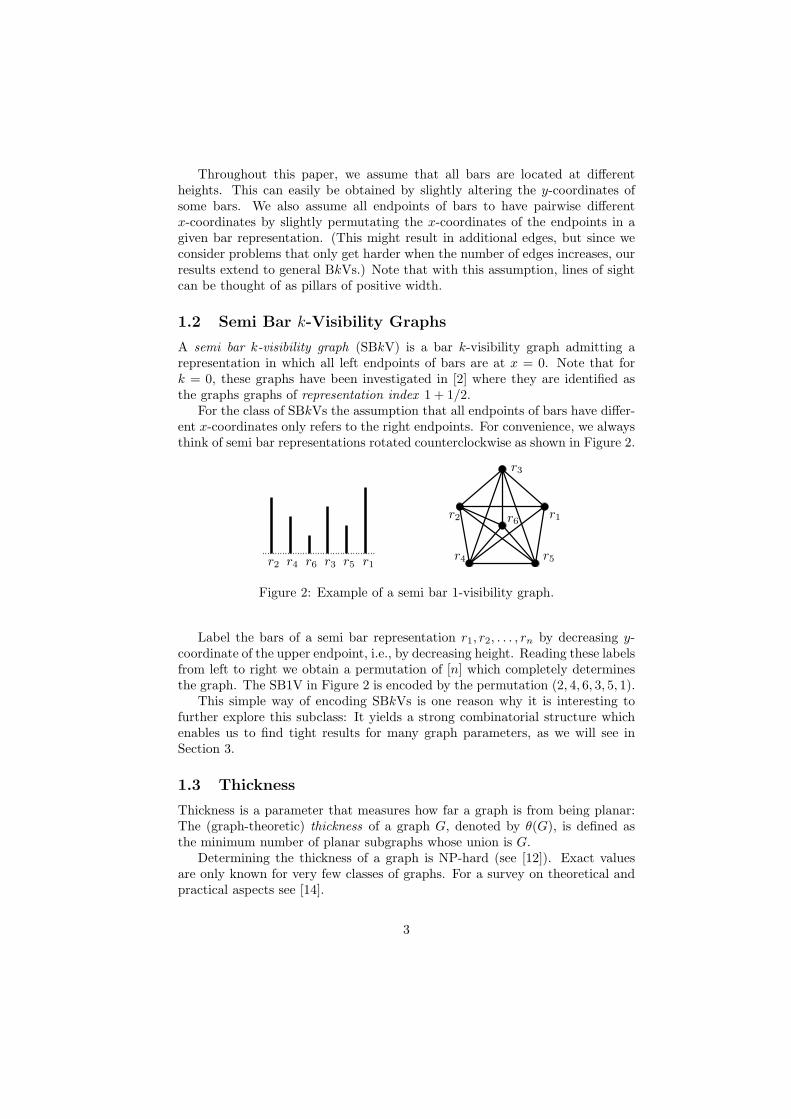
For the class of SBkVs the assumption that all endpoints of bars have differ-ent x-coordinates only refers to the right endpoints. For convenience, we alwaysthink of semi bar representations rotated counterclockwise as shown in Figure 2.

r1

r1r2

r2

r3

r3r4r4

r5r5

r6

r6

Figure 2: Example of a semi bar 1-visibility graph.

Label the bars of a semi bar representation r1, r2, . . . , rn by decreasing y-coordinate of the upper endpoint, i.e., by decreasing height. Reading these labelsfrom left to right we obtain a permutation of [n] which completely determinesthe graph. The SB1V in Figure 2 is encoded by the permutation (2, 4, 6, 3, 5, 1).

This simple way of encoding SBkVs is one reason why it is interesting tofurther explore this subclass: It yields a strong combinatorial structure whichenables us to find tight results for many graph parameters, as we will see inSection 3.

1.3 Thickness

Thickness is a parameter that measures how far a graph is from being planar:The (graph-theoretic) thickness of a graph G, denoted by θ(G), is defined asthe minimum number of planar subgraphs whose union is G.

Determining the thickness of a graph is NP-hard (see [12]). Exact valuesare only known for very few classes of graphs. For a survey on theoretical andpractical aspects see [14].

3

Note that in the definition of thickness, the planar embeddings of the sub-graphs do not have to coincide. The geometric thickness of G asks for the min-imum number of subgraphs/colors in the following setting: Choose a straight-line embedding of G and a coloring of the edges such that crossing edges havedifferent colors, the edges of each color then form a plane graph. Geometricthickness was introduced by Dillencourt, Eppstein and Hirschberg in [6]. In [7],Eppstein showed that graph-theoretic thickness and geometric thickness are noteven asymptotically equivalent.

2 A Bar 1-Visibility Graph with Thickness 3

In [3], Dean et al. used the Four Color Theorem to show that the thicknessof B1Vs is bounded by 4. They conjectured that the correct bound is 2. Inthis section we construct a B1V with thickness 3. We will often talk about a2-coloring of a graph G = (V, E), meaning a 2-coloring of the edges such thateach color class is the edge set of a planar graph on V . Given a 2-coloring (withblue and red) we define Gblue and Gred as the graphs on V with all blue and allred edges, respectively.

Here is a brief outline of the construction: First we analyze a quite simpletype of graph which has thickness 2 but with the property that every 2-coloringhas uniform substructures, so called lampions. Assuming that the original graphis large enough we can assume arbitrarily large lampions. In a second step weintroduce a series of slight perturbations into the original graph. It is shownthat most of these perturbations have to be incorporated into lampions and thenumber of perturbations in one lampion is proportional to its size. However alampion can only absorb a constant number of the perturbations. This yields acontradiction to the assumption that a 2-coloring exists.

We start with an Autobahn where we have heaped up the median strip:Consider the bar representation of the graph An shown in Figure 3. This graphhas four outer vertices A, B, C, D and a set Vinner of n inner vertices. Each innervertex vi is adjacent to all outer vertices, and additionally to the inner verticesvi−2, vi−1, vi+1 and vi+2.

AB

CD

...Vinner

v1v2v3v4

vn

Figure 3: The Autobahn-graph An

Since An contains a K4,n as subgraph we know that An is non-planar (as-suming n ≥ 3), hence, θ(An) ≥ 2. To show that θ(An) = 2 we let Gblue consist

4

of all direct edges and Gred consist of all indirect edges. Figure 4 shows thepartition.

A ABB

CCD D

Gblue Gred

· · ·· · ·· · ·v1 v1 v2v2 v3 v3 v4v5 v6

vn

Figure 4: A partition of An into two planar graphs.

Let Vinner = {v1, v2, . . . , vn}, such that the indices represent the order of theright endpoints of the bars from left to right. The inner neighbors of vi arevi−2, vi−1, vi+1 and vi+2. The graph G[Vinner] induced by the inner vertices ismaximal outerplanar with an interior zig-zag.

A lampion in a 2-coloring of An consists of a set W = {vi, vi+1, . . . vj} ofconsecutive inner vertices and a partition {S1, S2}, {S3, S4} of the four outervertices such that Gblue consists of all zig-zag edges of G[W ] and all edgesconnecting vertices from W with S1 and S2, while Gred consist of the two outerpaths of G[W ] and all edges connecting vertices from W with S3 and S4 (ofcourse exchanging red and blue again yields a lampion). The set W is the coreof the lampion. See Figure 5 for a lampion coloring of the core. Note thatFigure 4 shows a lampion with core Vinner together with the additional edgesbetween the four outer vertices.

· · · · · ·

G[W ]

vi

vi−1

vi−2

vi−3

vi−4 vi+2

vi+3vi+1

Figure 5: A lampion coloring of G[W ].

Lemma 1. For every k ∈ IN there is an n ∈ IN such that in every 2-coloring ofAn there is a W ⊂ Vinner with |W | ≥ k such that W is the core of a lampion.

Proof. Each inner vertex has four outer neighbors. Let us call an edge con-necting an inner and an outer vertex a transversal edge. Consider the bluetransversal edges; at each vertex there can be 0, 1, 2, 3 or 4 of them. But Gblue

is planar and therefore does not contain a K3,3. Thus, at most two inner verticescan have the same three outer neighbors in Gblue. There are

(

4

3

)

= 4 differenttriples of outer neighbors in Gblue, so there can be at most eight inner verticeswith more than two outer neighbors in Gblue. We might find another eight in

5

Gred. These irregular vertices break the sequence v1, v2, v3, . . . , vn of inner ver-tices of An into at most 17 pieces. By pigeon-holing, there must be at least onepiece with size n′ ≥ (n − 16)/17 such that in the induced 2-coloring of An′ allinner vertices are incident to exactly two blue and two red transversal edges.

Considering only the blue transversal edges of An′ , the resulting subgraphG′

blue is a subgraph of a blown-up K4 as illustrated in Figure 6. This subgraphis not arbitrary but has the property that every inner vertex has exactly twoincident edges.

A

BC

D

Figure 6: Blown-up K4.

Now it remains to planarly embed the inner edges of An′ , i.e. those ofG[V ′

inner]. To our disposition we have the ≤ 4 ‘large faces’ of the blown-upK4, which makes eight faces in total for the two planar graphs. In each ofthese faces we can embed at most three inner edges. There are other cases withfewer large faces which have in turn more inner vertices at the boundary. Inall cases it is impossible to embed more than 12 edges between inner verticeswith different outer neighbors in G′

blue, the red subgraph may contain another12 irregular edges. These at most 24 irregularities break the sequence of innervertices of An′ into at most 25 pieces, we remain with a 2-coloring of An′′ withn′′ ≥ (n′−24)/25 such that all inner vertices are incident to the same two outervertices in G′

blue and to the other two outer vertices in G′

red.We now have K2,n′′ as a subgraph in both G′′

blue and in G′′

red. The goodthing about this is that K2,n′′ has an (essentially) unique planar embedding.Consequences for the inner edges of An′ are exploited in the following facts.

Fact 1. Every inner vertex of An′′ has at most two incident inner edges of eachcolor.

It follows that the 2-coloring of An′′ induces a 2-coloring of G[V ′′

inner] such thateach color consists of a set of paths and cycles.

Fact 2. The set of blue inner edges of An′′ contains at most one cycle. Thesame holds for the red inner edges. If there is a monochromatic cycle, then it isa spanning cycle of V ′′

inner.

6

There is not much freedom for a 2-coloring of the inner edges of An′′ with theseproperties: We almost have a lampion coloring on G[V ′′

inner]. The exception isthat there can be a single Z-structure (see Figure 7) in one color.

· · ·· · ·

G[Vinner]

Figure 7: One Z-structure and no monochromatic cycle force all other colors.

Removing the Z-structure leaves two consecutive pieces of the sequence ofinner vertices. These pieces of V ′′

inner have a lampion coloring. The size of thelarger piece can be estimated as n′′′ ≥ (n′′ − 4)/2. This proves the lemma.

Well-prepared we can now look at the variant Bn of An in which we haveslightly perturbed some of the inner bars, see Figure 3.

AB

CD

...

Vinner

Figure 8: The modified Autobahn-graph Bn.

To obtain Bn, we have elongated every (say) tenth inner bar by pulling itsleft endpoint to the left, such that it is further left than the left endpoint ofthe bar directly above. With this modification we introduce an additional edgebetween the elongated bar vi and vi−3, but in turn we lose the edge betweenthe bar vi−1 and the lowest outer bar D. Let us call the vertices correspondingto the elongated bars modified vertices.

Theorem 2. The graph Bn is a bar 1-visibility graph with thickness 3, for nlarge enough.

Proof. We will show that Bn has no 2-coloring. It follows that its thicknessis at least 3, and since we can easily use a 2-coloring of An and embed theindependent additional edges in a third graph, B3 has thickness exactly 3.

Assume that Bn admits a 2-coloring. We first show that any 2-coloring ofBn would have to be very much alike a 2-coloring of An.

The vertices corresponding to a bar directly above a modified one – let uscall them reduced – have only three outer neighbors. To avoid a K3,3 in one color

7

there can be at most 16 inner vertices incident to more than two transversaledges. In particular, most reduced vertices have to divide their three incidenttransversal edges into two of one color and one of the other. As in the proof ofthe lemma we consider a continuous piece in the sequence of inner vertices suchthat all inner vertices have at most two transversal edges of each color. Thegraph induced by the largest of these pieces and the outer vertices is Bn′ .

The blue subgraph G′

blue of Bn′ is a subgraph of a blown-up K4 where atleast 9/10 of the inner vertices have degree 2 and the remaining reduced verticeshave degree 1. As in the proof of the lemma it can be argued that there is only aconstant number c of edges in G′

blue which join two inner vertices such that thereare at least three different outer neighbours of these two vertices, i.e., which jointwo inner vertices which not belonging to the same blown-up edge of K4. Theconstant can be bounded as c ≤ 24. The red graph may contribute another setof c irregular edges. Removing the irregularities will break the sequence of innervertices into at most 2c + 1 pieces. The graph induced by the largest of thesepieces and the special vertices is Bn′′ . Assuming that the edges between innervertices and D are blue in the 2-coloring of Bn′′ the transversal edges of G′′

blue

and G′′

red are shown in Figure 9.

· · · · · ·· · · · · · · · ·

D

vv

Figure 9: Embedding of a reduced vertex v in G′′

blue and G′′

red.

Let v = vi−1 be a reduced vertex, the neighbors vi and vi−3 of v both haveinner degree 5. In G′′

red they have degree (at most) 2, hence, they must havedegree 3 in G′′

blue. This is only possible if vi, vi−1 and vi−3 form a blue triangle.Since vi−1 can have no further blue inner neighbors it follows that the edgesvi−1vi−2 and vi−1vi+1 must be red.

Now consider the edge vi−2vi−3. Let us first suppose that this edge is coloredblue. To avoid closing a blue cycle, the edge vi−2vi must be red. Then to avoida red cycle the edge vivi+1 must be blue. Continuing that way the colors ofall edges to the right of the blue triangle in Figure 10 are uniquely determined.To the other side consider the parity of blue and red edges at vi−2, this forcesvi−2vi−4 to be blue, while the parity at vi−3 forces two red edges. To avoid ared cycle vi−4vi−5 must be blue, whence, parity forces vi−4vi−6 to be red. Thatway the color of edges left of the blue triangle is determined. The completepicture is shown in Figure 10: We have found a blue Z-structure.

Now suppose that the color of the edge vi−3vi−2 is red. Recalling thatvi−1vi−2 and vi−1vi+1 are red, consider the parity at vi−2 which forces vi−2vi

and vi−2vi−4 to be blue. Now, parity at vi forces the red edges vivi+1 and

8

· · · · · ·

vi

vi−1

vi−2

vi−3

vi−4

vi−5

vi+2

vi+1G[Vinner]

Figure 10: The blue edge vi−3vi−2 implies a blue Z.

vivi+2. Hence, we have a red Z-structure in this case, see Figure 11.

· · ·· · ·

vi

vi−1

vi−2

vi−3

vi−4

vi−5

vi+2

vi+1G[Vinner]

Figure 11: The red edge vi−3vi−2 implies a red Z.

We have seen that, given a modified vertex in Bn′′ , the parity condition andthe cycle-freeness of the colored graphs induced by the inner vertices of Bn′′

enforce a Z-structure. The zig-zag emanating from such a Z-structure in onedirection has to run into the Z-structure of a second modified vertex. The outerpaths of the other color make a turn at a modified vertex – and close a cycleat a second one. This is a contradiction since the blue triangles of the modifiedvertices are the only monochromatic cycles in G[V ′′

inner]. The contradiction showsthat for large1 n there is no 2-coloring of Bn, hence, the thickness of the graphis 3.

Our construction of a B1V with thickness 3 and the upper bound of 4 byDean et al. [3] leave a gap waiting to be closed. Considering that the graphof our proof only requires few independent edges in the third planar layer, thefollowing conjecture seems plausible:

Conjecture 1. The thickness of bar 1-visibility graphs is at most 3.

3 Parameters of Semi Bar k-Visibility Graphs

In this section we present some structural properties of semi bar k-visibilitygraphs, before turning to their thickness in Section 4. We will see why SBkVsform an interesting subclass of BkVs: Their strong combinatorial structure givesrise to a number of proof techniques yielding tight results for different graphparameters.

1A rough computation yields that n ≥ 25000 should do.

9

3.1 Basic Properties

Semi bar 0-visibility graphs are outerplanar, as observed in [2] (for a proofsee [13]). For k > 0, SBkVs in general are non-planar. Here we show that theyare (2k + 2)-degenerate, which is a useful property for limiting their minimumdegree and always provides a point of attack for induction proofs. We willsee that the upper bounds on the chromatic number and the clique number ofSBkVs follow easily.

Definition 3. A graph G is called ℓ-degenerate if every subgraph of G has avertex of degree at most ℓ.

Lemma 4. Semi bar k-visibility graphs are (2k + 2)-degenerate for all k ≥ 0.

Proof. The vertex corresponding to the shortest bar in a bar representationalways has degree at most 2(k + 1).

Corollary 5. The chromatic number of a semi bar k-visibility graph is at most2k + 3, for all k ≥ 0.

Proof. This can be seen with a standard inductive argument. For the inductionstep, take out a vertex v of degree 2k + 2, color the remaining graph, and usethe free color when re-inserting v.

Example 6. To see that there are SBkVs attaining the chromatic number 2k+3for all k ≥ 0, consider Figure 12 which shows a schematic bar representationof K2k+3. Note that for any complete graph on n ≤ 2k + 2 vertices, a barrepresentation can be found by leaving out some of the bars in Figure 12.

k + 1k + 1

Figure 12: A complete SBkV on 2k + 3 bars.

Corollary 7. The clique number of SBkVs is 2k + 3.

Proof. Since SBkVs are (2k + 2)-degenerate, no such graph can contain a com-plete subgraph on more than 2k + 3 vertices.

We have seen above that the largest possible chromatic number of SBkVscoincides with the size of the largest complete SBkV. However, this does nottransfer to every particular SBkV and its induced subgraphs.

Example 8. Figure 13 shows an SBkV containing C5 as induced subgraph.

Corollary 9. In general, SBkVs are not perfect.

10

v1 v2 v3 v4 v5kkkk

Figure 13: Example of a non-perfect SBkV: The vi form an induced C5.

3.2 Maximum Number of Edges

In this section, we show a tight upper bound for the maximum number of edgesin an SBkV, and we characterize the bar representations of SBkVs attainingthis bound.

Let us start with some edge counting. If an SBkV on n ≤ 2k + 3 verticesis given, then by Proposition 7 the tight upper bound on its number of edgesis

(

n2

)

. For n = 2k + 2 and n = 2k + 3 this bound coincides with the bound forlarger n given in the following theorem:

Theorem 10. A semi bar k-visibility graph on n ≥ 2k + 2 vertices has at most(k + 1)(2n − 2k − 3) edges.

Proof. Think of the edges as being directed from longer to shorter bars. Sinceeach bar has at most 2(k+1) longer neighbors, each vertex has at most 2(k+1)incoming edges. Thus we have a first upper bound of 2n(k + 1) on the numberof edges.

Let us look more closely at the longest bars: The vertex r1 correspondingto the longest bar does not have any incoming edges, r2 has at most one, r3

two, and so on until reaching r2k+2 which has no more than 2k + 1 incomingedges. Substracting these edges that we counted too many in our first boundfrom 2n(k + 1), we obtain the desired upper bound:

2n(k + 1) −

2k+2∑

i=1

i = 2n(k + 1) −1

2(2k + 2)(2k + 3) = (k + 1)(2n − 2k − 3)

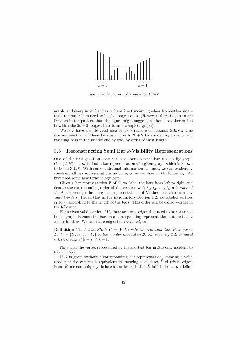
For any k ≥ 0 and n ≥ 2k + 2, semi bar k-visibility graphs with(k + 1)(2n − 2k − 3) edges exist. See Figure 14 for a schematic bar representa-tion of such a maximal SBkV : The k + 1 leftmost bars together with the k + 1rightmost bars form a complete graph. We call these bars outer bars and thecorresponding vertices outer vertices. Every shorter bar has k + 1 incomingedges from either side. Here we speak of inner bars and inner vertices.

Note that any maximal SBkV has to have a bar representation with thepattern described above. The 2(k + 1) outer bars have to induce a complete

11

. . .

k + 1k + 1

Figure 14: Structure of a maximal SBkV

graph, and every inner bar has to have k + 1 incoming edges from either side –thus, the outer bars need to be the longest ones. (However, there is some morefreedom in the pattern than the figure might suggest, as there are other ordersin which the 2k + 2 longest bars form a complete graph).

We now have a quite good idea of the structure of maximal SBkVs: Onecan represent all of them by starting with 2k + 2 bars inducing a clique andinserting bars in the middle one by one, by order of their length.

3.3 Reconstructing Semi Bar k-Visibility Representations

One of the first questions one can ask about a semi bar k-visibility graphG = (V, E) is how to find a bar representation of a given graph which is knownto be an SBkV. With some additional information as input, we can explicitelyconstruct all bar representations inducing G, as we show in the following. Wefirst need some new terminology here.

Given a bar representation B of G, we label the bars from left to right anddenote the corresponding order of the vertices with t1, t2, . . . , tn a t-order ofV . As there might be many bar representations of G, there can also be manyvalid t-orders. Recall that in the introductory Section 1.2, we labeled verticesr1 to rn according to the length of the bars. This order will be called r-order inthe following.

For a given valid t-order of V , there are some edges that need to be containedin the graph, because the bars in a corresponding representation automaticallysee each other. We call these edges the trivial edges :

Definition 11. Let an SBkV G = (V, E) with bar representation B be given.Let V = {t1, t2, . . . , tn} in the t-order induced by B. An edge titj ∈ E is calleda trivial edge if |i − j| ≤ k + 1.

Note that the vertex represented by the shortest bar in B is only incident totrivial edges.

If G is given without a corresponding bar representation, knowing a validt-order of the vertices is equivalent to knowing a valid set E of trivial edges:From E one can uniquely deduce a t-order such that E fulfills the above defini-

12

tion. In the following theorem, we need one of these informations as additionalinput.

Theorem 12. For k ≥ 0, let an SBkV G be given with a valid t-order of itsvertices. Then an r-order of the vertices can be computed which, together withthe given t-order, defines a bar representation inducing G.

Proof. The idea is to find a bar representation by first choosing a vertex whichwill be represented by the shortest bar, then deleting it from the graph, anditerating this until we have defined a complete r-order of the vertices.

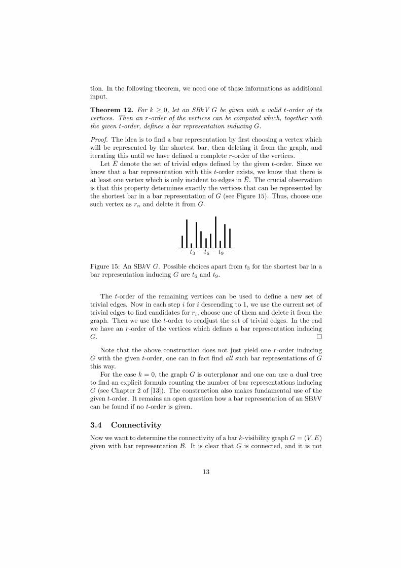
Let E denote the set of trivial edges defined by the given t-order. Since weknow that a bar representation with this t-order exists, we know that there isat least one vertex which is only incident to edges in E. The crucial observationis that this property determines exactly the vertices that can be represented bythe shortest bar in a bar representation of G (see Figure 15). Thus, choose onesuch vertex as rn and delete it from G.

t3 t6 t9

Figure 15: An SBkV G. Possible choices apart from t3 for the shortest bar in abar representation inducing G are t6 and t9.

The t-order of the remaining vertices can be used to define a new set oftrivial edges. Now in each step i for i descending to 1, we use the current set oftrivial edges to find candidates for ri, choose one of them and delete it from thegraph. Then we use the t-order to readjust the set of trivial edges. In the endwe have an r-order of the vertices which defines a bar representation inducingG.

Note that the above construction does not just yield one r-order inducingG with the given t-order, one can in fact find all such bar representations of Gthis way.

For the case k = 0, the graph G is outerplanar and one can use a dual treeto find an explicit formula counting the number of bar representations inducingG (see Chapter 2 of [13]). The construction also makes fundamental use of thegiven t-order. It remains an open question how a bar representation of an SBkVcan be found if no t-order is given.

3.4 Connectivity

Now we want to determine the connectivity of a bar k-visibility graph G = (V, E)given with bar representation B. It is clear that G is connected, and it is not

13

too hard to guess that its connectivity is k + 1, since any bar can see its k + 1left and k + 1 right neighbors.

Theorem 13. Semi bar k-visibility graphs on more than k + 1 vertices are(k + 1)-connected.

Proof. In order to separate the subgraph built by the trivial edges (cf. Def. 11)of G, a separating set has to contain at least k + 1 vertices.

k + 1

Figure 16: A bar representation containing a (k + 1)-separator

Figure 16 shows that in general an SBkV can have a (k + 1)-separator. Ifwe delete the k + 1 vertices corresponding to the bars in the middle, the graphfalls apart into the two components induced by the three bars on the left andthe remaining ones on the right side. There is an explicit way of characterizingthe (k + 1)-separators:

Proposition 14. Let G = (V, E) be an SBkV given with a bar representationB and a corresponding t-order of V . Let S ⊂ V . Then S is a (k + 1)-separatorof G if and only if S = {ti, ti+1, . . . , ti+k} for some i with 1 < i < n − k, andleft or right of B(S) in B all bars are shorter than the shortest one in B(S).

Proof. We first show that the two conditions are necessary for S to be a (k+1)-separator. In order to separate the subgraph built by the trivial edges of G,the vertices of S have to be successive in the t-order. Also, they must not belocated at one of its ends, else there would be nothing to separate. This provesthe first condition. Now let S = {ti, ti+1, . . . , ti+k} with 1 < i < n − k. LetB(tj) be the shortest bar in B(S). Suppose that left and right of B(S) there isa bar longer than B(tj). Let B(tℓ) be the rightmost such bar left of B(S), andlet B(tm) be the leftmost such bar right of B(S). Then there is a line of sightbetween B(tℓ) and B(tm), since there are at most k longer bars which couldcloud it. The edge tℓtm connects the two paths t1, . . . , ti−1 and ti+k+1, . . . , tn.Thus, S cannot be a separating set.

For the reverse direction observe that any set of vertices with the describedtwo properties separates the vertices corresponding to the “shorter half” of thebar representation from the rest of the graph (see Figure 16), and thus is a(k + 1)-separator.

Using the characterization of Proposition 14 one can efficiently find all the(k + 1)-separators of an SBkV which is given by a permutation defining a bar

14

representation. This is done by running through the vertices following thet-order, retaining the longest already seen and the longest not yet seen bar,and checking for each set of k + 1 successive bars if the shortest among them islonger than one of the two retained ones.

If we turn to maximal SBkVs, we get an even higher connectivity: By furtherexploring the structure of their bar representations one can see that they are2k + 2-connected. (This is the highest possible connectivity of an SBkV sincethe shortest bar has at most that many neighbors). The proof uses the globalversion of Menger’s Theorem and finds two (k+1)-bundles of independent pathsbetween any two vertices. The idea is nice and simple – every such path is builtby successively jumping k + 1 bars to the left (right). The whole proof in its(technical) details can be found in [13].

4 Thickness of Semi Bar 1-Visibility Graphs

Let G = (V, E) be an SB1V given by a bar representation, see e.g. Figure 2.In this section we present an algorithm which 2-colors the edges of G suchthat each color class forms a plane graph in an embedding induced by the barrepresentation. Consequently the thickness of an SB1V is at most 2.

Between the full class of B1Vs and the subclass of SB1Vs there is the class ofbar 1-visibility graphs admitting a representation by a set of bars such that thereis a vertical line stabbing all bars of the representation. Note that Theorem 2implies that already in this intermediate class there are graphs of thickness 3.

4.1 One-Bend Drawing

A one-bend drawing of a graph is a drawing in the plane in which each edgeis a polyline with at most one bend. Here we introduce a one-bend drawing ofSB1Vs with some specified properties. This drawing is not planar in general,but it will be helpful for the construction and the analysis of the 2-coloring.

Enlarge the bars of each vertex v to a rectangle B(v) with a uniform width.Recall that we assume that the heights of all bars are different and that B(r1),B(r2), . . . , B(rn) lists the bars by decreasing height. Assign the stripe betweenthe horizontal line touching the top of bar B(ri) and the horizontal line touchingthe top of bar B(ri−1) to ri. The dotted lines in Figure 17 separate the stripes.Embed each vertex v at the midpoint of the upper boundary of B(v). We thinkof the edges as being directed from the longer bar (its starting bar) to the shorterbar (its ending bar).

Now draw each edge e = rirj composed of two segments; the first segmentis contained in B(ri), it connects ri with the inflection point xe, the secondsegment connects xe with rj within the stripe of rj . Place xe on the verticalboundary of B(ri) which is closer to rj , with a height which is inside the stripeof rj . This position of xe bewares from crossings between edges emanatingfrom ri. We call the segment (ri, xe) the vertical part, the segment (xe, rj) thehorizontal part of the edge. Note that the stripe associated with B(v) contains

15

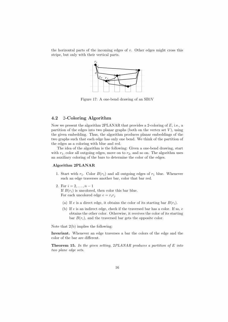
the horizontal parts of the incoming edges of v. Other edges might cross thisstripe, but only with their vertical parts.

e

ri

rjxe

Figure 17: A one-bend drawing of an SB1V

4.2 2-Coloring Algorithm

Now we present the algorithm 2PLANAR that provides a 2-coloring of E, i.e., apartition of the edges into two planar graphs (both on the vertex set V ), usingthe given embedding. Thus, the algorithm produces planar embeddings of thetwo graphs such that each edge has only one bend. We think of the partition ofthe edges as a coloring with blue and red.

The idea of the algorithm is the following: Given a one-bend drawing, startwith r1, color all outgoing edges, move on to r2, and so on. The algorithm usesan auxiliary coloring of the bars to determine the color of the edges.

Algorithm 2PLANAR

1. Start with r1. Color B(r1) and all outgoing edges of r1 blue. Wheneversuch an edge traverses another bar, color that bar red.

2. For i = 2, . . . , n − 1If B(ri) is uncolored, then color this bar blue.For each uncolored edge e = rirj

(a) If e is a direct edge, it obtains the color of its starting bar B(ri).

(b) If e is an indirect edge, check if the traversed bar has a color. If so, eobtains the other color. Otherwise, it receives the color of its startingbar B(ri), and the traversed bar gets the opposite color.

Note that 2(b) implies the following:

Invariant. Whenever an edge traverses a bar the colors of the edge and thecolor of the bar are different.

Theorem 15. In the given setting, 2PLANAR produces a partition of E intotwo plane edge sets.

16

Figure 18: A coloring produced by the algorithm 2PLANAR.

Proof. We have to show that in the 2-coloring computed by 2PLANAR, anytwo crossing edges have different colors.

The one-bend drawing implies that crossings between edges only appearbetween the vertical part of one edge and the horizontal part of another edge.Consider a crossing pair e, f of edges, assume that the crossing is on the verticalpart of e and the horizontal part of f . Hence, the crossing point is inside ofthe starting-bar of e, and the edge f is an indirect edge traversing this bar (seeFigure 19).

e1

e1

e2

e2

f1

f2

f2e

ef f

et = f1

et

Figure 19: Two crossing edges e and f , shown in two possible configurations.Note that there can be many shorter bars between the bars depicted here.

Let the start-vertex of e be e1 and its end-vertex e2. Similarly, let f leadfrom f1 to f2. Suppose that the color of f is red, then the invariant implies thatB(e1) is blue.

If e is a direct edge it obtains the color of its starting bar, in this case blue.Thus, assume that e is an indirect edge. Then its color depends on the colorof the traversed bar, let B(et) be this bar. (Note that et = f1 or et = f2 arepossible.)

The key for concluding the proof lies in the following lemma:

Lemma 16. If B(v) is an arbitrary bar, then at most one longer bar can be the

17

starting bar of indirect edges traversing B(v).

Proof. Assume that x = x1x2 is an edge traversing B(v) with B(x1) longer thanB(v), such that B(x2) is the shortest ending bar among all such edges. Thenwe know that between B(x1) and B(v) in the left-to-right-order there can beno bar longer than B(x2), else it would block the line of sight which correspondto x.

Suppose there is another edge y = y1y2 starting from a bar B(y1) which islonger than B(v). The choice of x implies that the horizontal part of y is abovethe horizontal part of x. Since y can traverse only one bar it must connect to abar B(yi) which is between B(v) and B(x1) in the left-to-right-order. Since yis above x the bar B(yi) is longer than B(x2). This is in contradiction to theconclusion of the previous paragraph. △

Now let us first assume that B(et) is shorter than B(e1). Then by the lemmawe know that B(e1) is the only longer bar sending an edge (e.g. the edge e)through B(et). Therefore B(et) is still uncolored when the algorithm considersB(e1), therefore, e is colored with the color of B(e1), which is blue. This showsthat the edges e and f have different colors in this case.

If B(et) is longer than B(e1), then we can deduce et = f1. For if a barlonger than B(et) would be located strictly between B(f1) and B(f2) in theleft-to-right-order, the line of sight corresponding to f would have to traversetwo bars (B(e1) and this longer bar), which is a contradiction. In addition, weknow that B(f2) is shorter than B(e1), else e and f would not cross. Thus, wehave et = f1, and B(f1) is longer than B(e1). In this case the lemma tells usthat B(f1) is the only longer bar sending an edge through B(e1). It follows thatB(e1) was still uncolored when algorithm considered B(f1). Therefore, the redcolor of f was chosen equal to the color of the bar B(f1). The invariant impliesthat the edge e, traversing the red bar B(f1), is blue. Hence, again e and fhave different colors.

The algorithm shows that SB1Vs have graph-theoretical thickness not morethan 2, and it defines a partition of the edges into two planar graphs, providingtwo plane embeddings. Since the positions of each vertex coincide in these twoembeddings, a natural question now is to ask whether we can also bound thegeometric thickness of SB1Vs. Recall that for geometric thickness, rectilinearplanar embeddings are needed (cf. Section 1.3). The following theorem showsthat we can turn our one-bend drawing into a straight-line embedding. Thistheorem confirms a conjecture from [8].

Theorem 17. The geometric thickness of SB1Vs is at most 2.

Proof. Let an SB1V G with a corresponding bar representation be given andreconsider the definition of a one-bend drawing of G. We change the height ofthe stripes Sj , with j increasing to n. In each step, we consider the incomingedges e = rirj of vertex rj . We let Sj be so high that the rectilinear connectionbetween ri and rj leaves the bar B(ri) in a point xe inside of Sj . See Figure 20as illustration.

18

exe

rj

ri

Sj

Figure 20: We let the stripe Sj be so high that the incoming edges of rj can bedrawn rectilinear.

Having done this for all stripes we obtain a straight-line embedding of Gwhere each edge e falls into its “vertical” part from vi to xe and its “horizontal”part from xe to rj . The vertical part runs inside of the bar B(ri) and thehorizontal part inside of the stripe Sj . This embedding is a one-bend drawing asdefined in Section 4.1 (with the additional property that all edge-bends have anangle of 180 degree). Thus by Theorem 15 the algorithm 2PLANAR partitionsthis drawing into two plane layers.

4.3 Structure of the Blue and Red Graph

Given a semi bar 1-visibility graph G = (V, E), we can say more about the effectof the algorithm 2PLANAR on G: It partitions the edges evenly among the blueand the red graph. As blue graph let us define Gblue := (V ′, Eblue) by takingall blue edges on the vertex set V and deleting isolated vertices. The red graphis defined analogously as Gred := (V ′′, Ered). Recall that from Theorem 10 weknow that an SB1V has at most (k + 1)(2n − 2k − 3) = 4n − 10 edges.

Proposition 18. The blue and the red graph each contain at most 2n−3 edges.

Proof. We count the incoming blue edges at each vertex and claim that thereare at most two of them. See Figure 21 for an illustration. Consider a bar B(v)and the closest bar to the left (say) of it that is the starting bar B(w) of anincoming blue edge at v. Either such an edge springs from a direct line of sightbetween B(v) and the blue bar B(w), or it is induced by an indirect line of sighttraversing a red bar B(u).

In the first case, any other incoming blue edge from the left has to traverseB(w) and therefore is colored red. In the second case, any other such edgewould have to traverse B(w) as well as B(u), which is not possible.

Thus there is at most one incoming blue edge from each side, which yieldsan upper bound of 2n blue edges. But the vertex r1 represented by the longestbar has no incoming edges, and r2 has only one. Therefore we can substractthree edges, obtaining the desired result. The same argument applies to thenumber of red edges.

19

Figure 21: Example of an SB1V with 2n − 3 blue edges.

The upper bound of Proposition 18 is sharp, as the blue graph in Figure 21shows: Any vertex except for r1 and r2 has two incoming edges. The patternshown by the example in the figure can be used to construct an SB1V with2n − 3 blue edges for arbitrary n.

The edge bound of 2n− 3 may sound familiar – it also holds for outerplanargraphs. However, the example in the figure shows that, in general, Gblue andGred are not outerplanar: The blue graph induced by the five longest bars formsa K2,3. In Figure 22, the red graph induced by the vertices t2, t3, t5, t6 and t7contains K4 as a minor, which can be obtained by contracting the edge t3t5.

t1

t2

t3

t4

t5

t6

t7

t8

Figure 22: The red graph contains K4 as a minor.

For the case of maximal SB1Vs, there is more structure to explore withinthe blue and the red graph defined by 2PLANAR. In fact it can be shown (see[13]) that in this case they are both Laman graphs, which implies a number ofadditional properties.

20

5 Conclusion and Open Problems

In this paper, we disproved the conjecture of Dean et al. [3] that the tight upperbound on the thickness of bar 1-visibility graphs is 2.

On the way of getting a better understanding of bar k-visibility graphs weconsidered semi bar k-visibility graphs which have a strong combinatorial struc-ture. We used this structure to get tight bounds on the clique number, the chro-matic number, the maximum number of edges and the connectivity of SBkVs.For the case k = 1, we proved the tight upper bound of 2 on the thickness ofSBkVs, confirming the conjecture of Dean et al. for this subclass.

Still, many questions are left open, and new ones emerged. The followingopen problems may serve as a starting point for further research.

1. In [3], it is shown that the thickness of BkVs can be bounded by a functionin k (proven is a quadratic one). What is the smallest such function?

2. What is the largest thickness or geometric thickness of SBkVs?

3. What is the largest chromatic number of BkVs? Dean et al. show an upperbound of 6k + 6.

4. Hartke, Vandenbussche and Wenger [9] found some forbidden induced sub-graphs of BkVs. They ask for further characterization of BkVs by forbid-den subgraphs.

5. Hartke et al. also examined regular BkVs. Are there d-regular BkVs ford ≥ 2k + 3?

6. What is the largest crossing number of BkVs?

7. What is the largest genus of BkVs?

8. How can SBkVs be characterized?

9. Can SBkVs be recognized in polynomial time?

Acknowledgments

We thank Gunter Rote for a hint leading to the proof of Theorem 17.

References

[1] P. Bose, A. M. Dean, J. P. Hutchinson, and T. C. Shermer, Onrectangle visibility graphs, in Proceedings of Graph Drawing ’96, vol. 1353of Lecture Notes Comput. Sci., Springer, 1997, pp. 25–44.

[2] F. J. Cobos, J. C. Dana, F. Hurtado, A. Marquez, and F. Mateos,On a visibility representation of graphs, in Proceedings of Graph Drawing’95, vol. 1027 of Lecture Notes Comput. Sci., Springer, 1995, pp. 152–161.

21

[3] A. M. Dean, W. Evans, E. Gethner, J. D. Laison, M. A. Safari,

and W. T. Trotter, Bar k-visibility graphs. Manuscript, 2005.

[4] , Bar k-visibility graphs: Bounds on the number of edges, chromaticnumber, and thickness, in Proceedings of Graph Drawing ’05, vol. 3843 ofLecture Notes Comput. Sci., Springer, 2006, pp. 73–82.

[5] A. M. Dean, E. Gethner, and J. P. Hutchinson, Unit bar-visibilitylayouts of triangulated polygons., in Proceedings of Graph Drawing ’04,vol. 3383 of Lecture Notes Comput. Sci., Springer, 2005, pp. 111–121.

[6] M. B. Dillencourt, D. Eppstein, and D. S. Hirschberg, Geometricthickness of complete graphs, J. Graph Algorithms & Applications, 4 (2000),pp. 5–17. Special issue for Graph Drawing ’98.

[7] D. Eppstein, Separating thickness from geometric thickness, in Proceed-ings of Graph Drawing ’02, vol. 2528 of Lecture Notes Comput. Sci.,Springer, 2002, pp. 150–161.

[8] S. Felsner and M. Massow, Thickness of bar 1-visibility graphs, inProceedings of Graph Drawing ’06, vol. 4372 of Lecture Notes Comput.Sci., Springer, 2007, pp. 330–342.

[9] S. G. Hartke, J. Vandenbussche, and P. Wenger, Further resultson bar k-visibility graphs. Manuscript, November 2005.

[10] J. P. Hutchinson, Arc- and circle-visibility graphs, Australas. Journal ofCombin., 25 (2002), pp. 241–262.

[11] J. P. Hutchinson, T. Shermer, and A. Vince, On representationsof some thickness-two graphs, Comput. Geom. Theory Appl., 13 (1999),pp. 161–171.

[12] A. Mansfield, Determining the thickness of graphs is NP-hard, Math.Proc. Camb. Phil. Soc., 9 (1983), pp. 9–23.

[13] M. Massow, Parameters of bar k-visibility graphs. Diploma thesis, Tech-nische Universitat Berlin, 2006. www.math.tu-berlin.de/˜massow.

[14] P. Mutzel, T. Odenthal, and M. Scharbrodt, The thickness ofgraphs: A survey, Graphs and Combinatorics, 14 (1998), pp. 59–73.

[15] R. Tamassia and I. G. Tollis, A unified approach to visibility repre-sentations of planar graphs, Discrete Computational Geometry, 1 (1986),pp. 321–341.

[16] S. K. Wismath, Characterizing bar line-of-sight graphs, in Proceedings ofSCG ’85, ACM Press, 1985, pp. 147–152.

22