Parameterization and Applications of

Catmull-Rom Curves

Cem Yuksel, Scott Schaefer, John Keyser

3112 Texas A&M UniversityCollege Station, TX 77843-3112

Abstract

The behavior of Catmull-Rom curves heavily depends on the choice of pa-rameter values at the control points. We analyze a class of parameterizationsranging from uniform to chordal parameterization and show that, withinthis class, curves with centripetal parameterization contain properties thatno other curves in this family possess. Researchers have previously indi-cated that centripetal parameterization produces visually favorable curvescompared to uniform and chordal parameterizations. However, the mathe-matical reasons behind this behavior have been ambiguous. In this paperwe prove that, for cubic Catmull-Rom curves, centripetal parameterizationis the only parameterization in this family that guarantees that the curvesdo not form cusps or self-intersections within curve segments. Furthermore,we provide a formulation that bounds the distance of the curve to the controlpolygon and explain how globally intersection-free Catmull-Rom curves canbe generated using these properties. Finally, we discuss two example appli-cations of Catmull-Rom curves and show how the choice of parameterizationmakes a significant difference in each of these applications.

Keywords: Catmull-Rom splines, parameterization, chordalparameterization, centripetal parameterization, uniform parameterization,animation curves, path curves

1. Introduction

Catmull-Rom curves are widely used in graphics for a variety of appli-cations ranging from modeling to animation. These parametric curves havethree important properties that make them so popular. First, the curves

Preprint submitted to Computer-Aided Design August 23, 2010

(a) Uniform

(b) Chordal

(c) Centripetal

Figure 1: Cubic Catmull-Rom curves with (a) uniform, (b) chordal, and (c) cen-tripetal parameterization. While uniform and chordal parameterizations can produceself-intersections, centripetal parameterization is the only one that guarantees no self-intersections within curve segments.

are smooth and interpolate their control points, which gives the user directcontrol over various points on the curve. Second, the curves have local sup-port, so that each control point only affects a small neighborhood on thecurve. Finally, Catmull-Rom curves have an explicit piecewise polynomialrepresentation, allowing them to be easily be converted to other bases andmanipulated computationally.

Perhaps the most popular parameterization of Catmull-Rom curves isa uniform parameterization (i.e. the control points are equally spaced inparametric space). However, this choice of parameterization does not reflectthe Euclidean distance between control points well. For curves with differentlength segments, this parameterization can lead to artifacts such as cusps andself-intersections, which occur frequently (Figure 1a). Moreover, the distanceof the curve from the control polygon can be unbounded, which makes thesecurves difficult to control in practice.

An alternative is to automatically create the parameterization of the curvefrom its geometric embedding in Euclidean space. Doing so gives rise to other

2

(a) (b)

(c) (d)

Figure 2: Catmull-Rom curves generated using the same control polygon (a) with differentparameterizations. Uniform parameterization (b) overshoots and often generates cuspsand intersections within short curve segments, while chord-length parameterization (c)exhibits similar behavior for longer curve segments. Centripetal parameterization (d) isthe only one that guarantees no intersections within curve segments.

known curve parameterizations such as chordal and centripetal parameteri-zations (Figure 1bc). However, like uniform parameterization, most param-eterization choices still produce the same artifacts observed with uniformparameterization (cusps, self-intersections, etc...).

Researchers have previously compared uniform, chordal, and centripetalparameterizations for various curves [1, 2, 3, 4] and observed that, amongthese three parameterization choices, centripetal parameterization producesvisually favorable curves. Yet, the reasoning behind this preference has beenlimited to informal explanations based on intuition, rather than a more for-mal mathematical explanation. Floater [5] does provide some evidence that,among these three parameterizations, centripetal parameterization producescurves closer to the control polygon for cubic splines than uniform or chordalparameterization. However, centripetal parameterization can be consideredas just one choice within an infinite family of parameterization choices be-tween uniform and chordal. Therefore, there may exist some other param-eterization that would produce even more favorable results than centripetalparameterization.

3

In this paper, we concentrate on cubic Catmull-Rom curves and analyzethe full class of parameterizations ranging from uniform to chordal parame-terization, such that the parameterization is a function of the length betweentwo consecutive control points. We show that centripetal parameterization,which is at the center of this class, inherits some important properties thatno other parameterization in this class possesses for these curves. Following abrief overview of Catmull-Rom curves in Section 2, in Section 3 we mathemat-ically prove that centripetal parameterization of Catmull-Rom curves guar-antees that the curve segments cannot form cusps or local self-intersections,while such undesired features can be formed with all other possible param-eterizations within this class. Furthermore, we provide a formulation thatbounds the distance between the control polygon and the actual curve inSection 4. Based on these two properties we derive rules to achieve globallyintersection-free Catmull-Rom curves in Section 5. In Section 6, we providea discussion of our results and observations. Finally, we explain the effectof parameterization in two applications of Catmull-Rom curves in Section 7,before we conclude in Section 8.

2. Background

Catmull-Rom curves were first described in [6] as a method for generatinginterpolatory curves with local support by combining Lagrange interpolationand B-spline basis functions. Barry and Goldman [7] exploited this relation-ship to show how to construct non-uniform Catmull-Rom curves by factoriz-ing the computation into a pyramid. Let Pi ∈ Rm be the control points of aCatmull-Rom curve and each control point be associated with the parametricvalue si. A Ck Catmull-Rom curve is composed of polynomial segments ofdegree 2k + 1 between consecutive control points. These polynomial piecesare only affected by a local set of control points. The polynomial piece ofthe curve between si and si+1 is influenced by control points Pi−k throughPi+1+k. Furthermore, the curve is interpolatory (i.e. at si and si+1, the curveevaluates to Pi and Pi+1 respectively).

We concentrate on C1 cubic Catmull-Rom curves as they are the simplestand most popular form of these curves. Figure 3 shows Barry and Goldman’spyramid algorithm for cubic Catmull-Rom curves that builds the polynomialC12(s) for the curve segment between parameter values s1 and s2. Thispyramid is composed of triangles with two points at the base and arrowswith coefficients leading to its apex. This notation should be interpreted as

4

C12s2−ss2−s1

s−s1s2−s1

L012 L123s2−ss2−s0

s−s0s2−s0

s3−ss3−s1

s−s1s3−s1

L01 L12 L23s1−ss1−s0

s−s0s1−s0

s2−ss2−s1

s−s1s2−s1

s3−ss3−s2

s−s2s3−s2

P0 P1 P2 P3

Figure 3: Cubic Catmull-Rom curve formulation.

multiplying each point at the base of the triangle by the coefficient on thearrow and summing the result. From this diagram, it is easy to see thatC1 Catmull-Rom curves are cubic polynomials as there are 3 levels in thispyramid and each adds a single, linear factor.

Notice that Barry and Goldman’s description of the Catmull-Rom curveis non-uniform and allows for arbitrary si values. The choice of these si iswhat we refer to as the parameterization of the Catmull-Rom curve. Thebehavior of these curves depends significantly on the parameterization asshown in Figure 2. Various parameterization methods have been developedpreviously [4, 8, 9] and we analyze a class of parameterizations described by[4] ranging from uniform to chordal parameterization where we define theparameter values as

si+1 = |Pi+1 −Pi|α + si , (1)

and s0 = 0, where 0 ≤ α ≤ 1. Note that when α = 0, the parameterization isuniform, and when α = 1, the parameterization becomes the chordal param-eterization. Similarly, α = 1

2corresponds to centripetal parameterization.

3. Cusps and Self-Intersections

Cusps and self-intersections are very common with Catmull-Rom curvesfor most parameterization choices. In fact, as we will show here, the only pa-rameterization choice that guarantees no cusps and self-intersections withincurve segments is centripetal parameterization.

To determine if a curve segment of the Catmull-Rom curve has aself-intersection, we will convert the polynomial to Bezier form. LetP0,P1,P2,P3 be four consecutive control points of the Catmull-Rom curvewith parameter values 0, dα1 , d

α2 + dα1 , d

α3 + dα2 + dα1 , where di = |Pi −Pi−1|

as shown in Figure 4. The control points of the cubic Bezier curve Bj

5

Figure 4: Control points Bj of the cubic Bezier curve constructed from cubic Catmull-Romcurve segment with control points Pi.

(j ∈ {0, 1, 2, 3}) representing this polynomial between dα1 and dα2 + dα1 , repa-rameterized to lie in the range [0, 1] are then

B0 = P1

B1 =d2α1 P2−d2α

2 P0+(2d2α1 +3dα

1 dα2 +d2α

2 )P1

3dα1 (dα

1 +dα2 )

B2 =d2α3 P1−d2α

2 P3+(2d2α3 +3dα

3 dα2 +d2α

2 )P2

3dα3 (dα

3 +dα2 )

B3 = P2.

(2)

A smooth curve will not have cusps or self-intersect on the parameterrange [0, 1] if there exists a line such that the curve projected onto thisline has derivative greater than zero over that interval [10]. Our choice ofprojection will be the line connecting B0 and B3 as this is the only choicethat is applicable to curves of all dimensions. Note that this condition withour choice of projection is both a necessary and sufficient condition for 1Dcurves (i.e. when the Bj are co-linear), and is a necessary but not sufficientcondition for higher dimensions.

We will first show that parameterizations other than centripetal can pro-duce cusps and self intersections by analyzing the derivative of the curve atthe endpoints. We will then show that for centripetal parameterization, it isnot possible to produce cusps or self intersections.

Theorem 1. For parameterizations of cubic Catmull-Rom curves other thancentripetal, the projected derivative may be negative at the end-points.

Proof. Given that our curve is a cubic and that the axis we have chosenconnects the two end-points of the Bezier curve, we need only consider thevector B1 −B0 in relationship to our chosen axis (B2 −B3 follows through

6

symmetry). Hence if (B1−B0) · (B3−B0) < 0, then the projected derivativewill begin negative (the direction of the derivative of a Bezier at its end-points is given by the vector from the end-point to the adjacent controlpoint). Expanding this expression using Equation 2 and the property thatdi = |Pi −Pi−1|, yields

d2α1 d

22 − d2α+1

2 d1 cos(θ)

3dα1 (dα1 + dα2 )< 0 (3)

where θ is the angle between P0 − P1 and P2 − P1 as shown in Figure 4.The left-hand side of this inequality achieves its minimum when cos(θ) = 1and the expression simplifies to

d2α1 d2 < d1d

2α2 .

When α < 12, this expression is satisfied when d2 < d1. When α > 1

2,

this expression is satisfied when d1 < d2. The only value of α that cannotmeet this inequality is α = 1

2. Hence, the centripetal parameterization is the

only parameterization for which the projected derivative at the endpoint isalways non-negative.

Since the derivative must be positive somewhere for the curve to reachB3 and the derivative is continuous, a negative derivative at the endpointimplies that a cusp or self intersection can be created. Thus, centripetalparameterization offers the only possibility for avoiding cusps and local selfintersections.

This test, however, is not sufficient to show that centripetal parameteri-zation cannot produce cusps within a single polynomial. We will show thisproperty in two stages, first by proving a general property regarding cuspformation, and then by showing that centripetal parameterization meets therequirements of that property.

Theorem 2. A cubic Bezier curve whose interior control points project to bewithin the open interval defined by the end-points of the Bezier curve cannothave a cusp or self-intersection.

Proof. Since Bezier curves are affinely invariant, we can assume without lossof generality that B0 is at the origin and B3 is on the x-axis at x = 1. Thecontrol points for the projected curve will be univariate values as well andthe control points for the projected Bezier curve are then (0, x1, x2, 1) where

7

x1, x2 are the x components of B1 and B2. Our goal is to show that thisprojected curve cannot have a zero derivative over this interval.

To this end, we construct the control points of the derivative of this curve,which is a quadratic Bezier curve with control points (3x1, 3(x2−x1), 3−3x2).Our assumption in the theorem states that 0 < x1 < 1 and 0 < x2 < 1.Therefore, there are two cases to consider: x1 ≤ x2 and x1 > x2.

If x1 ≤ x2, then the control points of the derivative curve are all greaterthan or equal to zero and, by the convex hull property of Bezier curves, thederivative is greater than zero.

If x1 > x2, then we can solve for the minimum of this quadratic Bezierpolynomial, which is

3(x1(1− x1) + x2(x1 − x2))

1 + 3(x1 − x2).

Notice that the denominator is always positive, since x1 > x2. Furthermore,x1(1 − x1) > 0 because 0 < x1 < 1, and x2(x1 − x2) > 0 since 0 < x2

and x1 > x2. Therefore, the numerator is always positive as well and thederivative is always greater than zero.

Theorem 2, assumes that the projection of the interior control points liesin the range (0, 1). We must show this is the case for centripetal parameter-ization.

Theorem 3. For centripetal parameterization of cubic Catmull-Rom curves,the interior control points of a cubic Bezier curve may not project beyond theouter control points.

Proof. We can again consider only the case of B1 (since B2 follows by sym-metry). Consider the projected magnitude of B1−B0 onto the edge definedby the end-points of the Bezier curve.

(B1 −B0) · (B3 −B0)

|B3 −B0|2.

If B1 projects onto the open interval defined by B0 and B3, then this quantitymust be within the range (0, 1). By Theorem 1, the numerator is non-negativeand, hence, this quantity is greater than or equal to 0. The case when thisquantity is equal to 0 corresponds to B1 = B0, which can indeed happen.However, this boundary case does not indicate a cusp as the derivative is

8

only zero exactly at the end-point. Therefore, to apply Theorem 2, we onlymust show that this quantity cannot satisfy

(B1 −B0) · (B3 −B0)

|B3 −B0|2≥ 1.

Using Equation 2 and letting r = d1/d2 be the ratio between the lengthsof consecutive segments of the control polygon, this expression simplifies to

rα − r1−α cos(θ)

3(1 + rα)≥ 1. (4)

This expression will be maximal when cos(θ) = −1. Using this substitutionand rewriting the expression yields

r1−α ≥ 3 + 2rα.

For 12≤ α ≤ 1 this expression is obviously false.

Thus, Theorem 2 guarantees that centripetal parameterization cannotproduce cusps or self-intersections. Theorem 1 shows that this is the onlyparameterization of cubic Catmull-Rom curves with that guarantee.

4. Distance Bound

A commonly desired property in all of geometric modeling is that thecontrol structure should provide some intuition about the shape being mod-eled. One typical way that this is expressed is that a curve should behave“similarly” to its control polygon. Other researchers [5] have also noted thata good interpolatory curve is one that does not deviate far from its controlpolygon. Thus, we would like to have a way to measure the possible deviationof a curve from its control polygon.

Consider the curve segment from P1 to P2 with Bezier points given byEquation 2. We will bound the distance of this curve to the line segmentcontaining its end-points. To do so, we first bound the distance of the curveto the infinite line containing its end-points as a lower bound to the distanceto the line segment itself.

To bound this distance to the infinite line, we first bound the distance ofB1 and B2 to this line. Again, via symmetry, we only need to consider B1’s

9

distance to the infinite line

h1 =

√|B1 −B0|2 −

((B1 −B0) ·

(B3 −B0)

|B3 −B0|

)2

=d2α

2 d1 |sin(θ)|3(dα1 + dα2 )dα1

Substituting r = d1/d2 yields

h1 = d2r1−α |sin(θ)|

3(1 + rα). (5)

Furthermore, the distance of a cubic Bezier curve to the infinite line contain-ing its end-points is bounded by 3

4the distance of its control points to that

line. Using this fact and the property that |sin(θ)| ≤ 1, we can bound thedistance h of any point on the curve to the infinite line by

h ≤ d2r1−α

4(1 + rα). (6)

Notice that, for α < 12, this distance is potentially unbounded for arbi-

trary r. That is, for such parameterizations, we cannot bound the distanceof the curve from the control polygon. However, for α ≥ 1

2, this distance

will be bounded solely as a fraction of the length of the edge (independent ofr). For example, for both centripetal parameterization (α = 1

2) and chordal

parameterization (α = 1) the distance of the curve segment to the infiniteline contained by its end-points is no more than 1

4times the length of the

edge. The minimal bound (independent of r) is achieved when α = 23

wherethe ratio is 1

8times the length of the edge.

While centripetal and chordal parameterizations have similar bounds tothe infinite line segments, they behave much differently in practice. For12≤ α < 2

3, the maximal distance ratio is achieved for r > 1 meaning that

the line segment we are bounding distance to is smaller than its adjacent linesegments (i.e. d2 is relatively small). For 2

3< α ≤ 1, the maximal distance

ratio is achieved for r < 1, which is the case in which the line segment weare bounding distance to is large in comparison to the adjacent line segments(i.e. d2 is relatively large). Since the bound in Equation 6 is related to thelength of the line segment, d2, the curve using chordal parameterization willappear farther away from the control polygon than the curve with centripetal

10

α = 12

α = 12

α = 23

α = 23

α = 1 α = 1

Figure 5: Bounding volumes for cubic Catmull-Rom curves with different α values. Boundson the right column are computed using the length of the corresponding segment only, sothat they represent maximum possible bound for the segment. Bounds on the left columnalso uses the lengths of neighboring segments using equations 6 and 8; therefore, they aremore tight. Note that centripetal parameterization (α = 1

2 ) does not need circular boundsat the control points, because the curve is always confined in the boxes aligned with theedges of the control polygon.

parameterization, in absolute distance. In fact, for 12≤ α ≤ 2

3, the limit

curve will never be farther than 18

the length of the longest line segment inthe control polygon and will typically be smaller. This effect can be seen inFigure 2, where the distance of the chordal curve is much further from thecontrol polygon than the centripetal curve.

However, simply bounding the distance of the curve segment of a Cat-mull-Rom curve to the infinite line containing its end-points is not sufficientto bound the distance of the curve to the line segment of the control polygon.When the interior Bezier points project outside of the line segment definedby B0 and B3, we must consider the distance of the control point B1 to itsclosest end-point. Notice that, by the discussion in Section 3, 1

2≤ α ≤ 1

implied that B1 will never project outside the interval on the side of itsopposite control point B3. Therefore, we only need to consider the length ofthe edge B1 −B0 to bound the distance of the curve to the end-point of theline segment.

11

We start by computing the angle θ at which the vector B1−B0 becomesperpendicular to B3 − B0. This is the point at which we must start usingthe distance l1 to the end-point B0 rather than the infinite line to bound thedistance to the line segment. From the expression in Equation 3, we can findthat

cos(θ) > r2α−1 . (7)

If we compute the length squared of the edge B1 −B0, we obtain

l21 = |B1 −B0|2 =d2

2(r2 + r4α − 2 cos(θ)r1+2α)

9r2α(1 + rα)2.

Notice that this equation depends on θ and is larger as cos(θ) decreases. Com-bining this equation with the inequality constraints on cos(θ) from Equation 7and taking the square root of the expression, we can bound the maximal dis-tance to the end-point as

l1 ≤d2

√r2 − r4α

3rα(1 + rα). (8)

This expression is identically 0 for α = 12

meaning that a Catmull-Romcurve with centripetal parameterization can be bounded solely using bound-ing boxes extruded in the perpendicular direction of its line segments. How-ever, for α = 1, this bound can be as high as 1

3the length of the line segment.

Therefore, for most curves we need not only bounding boxes around line seg-ments but spheres around vertices to bound the curve completely. Figure 5shows a 2D example of such bounding volumes. The figure demonstratesboth the local bounds considering only the length of the line segment, aswell as tighter bounds achieved by a (less local) evaluation of the lengths ofadjacent segments using equations 6 and 8.

5. Intersection-free Curves

Our goal here is to develop criteria that result in intersection free Cat-mull-Rom curves. There are three cases to consider: the local case wherewe must avoid cusps and self-intersections within a single polynomial, theadjacent case where we consider intersection between adjacent polynomials,and the g lobal case where different polynomial segments not adjacent to oneanother may intersect.

12

Figure 6: Bezier control polygons of two neighboring curve segments.

In Section 3 we showed that by using centripetal parameterization we canguarantee that the curve will not contain cusps or self-intersections withincurve segments, satisfying the local case. Also, as shown in section 4, wehave a bounding box that defines limits on the distance of the curve from thecorresponding segment of the control polygon. As long as we use a centripetalparameterization and avoid overlapping bounding boxes, the curve will notself-intersect. This satisfies the global case.

Unfortunately, we cannot use the same bounding boxes to deal with theadjacent case, since bounding boxes of adjacent segments will always overlap.Therefore, we must have an alternative means of ensuring that such adjacentsegments do not intersect. We do this by constructing an angular bound onthe control polygon of the curve.

Consider the two Bezier curves in Figure 6 that have control pointsB1

0,B11,B

12,B

13 and B2

0,B21,B

22,B

23 where B1

3 = B20 corresponding to two dif-

ferent curve segments of the Catmull-Rom curve with centripetal parame-terization. A Bezier curve lies within the convex hull of its control points,hence our intersection criteria will simply guarantee that the convex hullsdo not intersect. Notice that each convex hull (shown shaded gray in the

13

figure) contains its end-points. Furthermore, we can exclude the points B12

and B21 as they are necessarily co-linear and will lie on opposite sides of the

“V” formed by the control polygon.Therefore, we need only consider the hull formed by B1

0,B11,B

13 intersected

with the hull formed by B20,B

22,B

23. There are three cases to consider: B1

1

and B22 both lie on the outside of the “V”, B1

1 is on the inside of the “V” andB2

2 is on the outside (the symmetric case follows), and the case where bothB1

1 and B22 are on the interior (as illustrated in Figure 6).

For the first case, the portion of the convex hull we need to avoid inter-secting consists only of the edges of the control polygon. It is not possibleto have a self-intersection in such cases, since the curves are bounded awayfrom each other.

The other two cases are very similar, and so we will analyze the convexhull for only one side. We will bound the angle γ between B1

1 − B13 and

B10 − B1

3. First, we compute the length of the projection of B11 − B1

3 ontoB1

0 −B13. Using Equation 4, this length is given by

d2 − d2r1−α cos(θ)

3 + 3rα.

The ratio involving this length and the distance of B11 to the line segment

formed by B10 and B1

3 will be tan(γ). Combining this expression with Equa-tion 5 when α = 1

2, we obtain

tan(γ) =

√r |sin(θ)|

3 + 2√r −√r cos(θ)

.

Maximizing this function we find that γ ≤ π6; that is, the curve will extend

beyond the control polygon toward the interior of the “V” within an angleof π

6.

Therefore, when both B11 and B2

2 are on the interior of the “V”, the anglethat will guarantee no intersection between adjacent curve segments is π

3.

This bound, in combination with the global intersection test from Section 4,allows us to guarantee an intersection free Catmull-Rom curve when usingcentripetal parameterization.

To summarize, we form intersection-free curves as follows:

1. We use a centripetal parameterization to avoid self intersections withina curve segment.

14

2. To avoid intersections between adjacent curve segments, we restrict theangular bound of adjacent control polygon segments to be greater thanπ3, as described in this section.

3. We avoid intersections between other curve segments by not allowingoverlap between bounding boxes for non-adjacent segments.

6. Discussion

As a result of our theoretical and experimental analysis, we had severalobservations about Catmull-Rom curves. In this section we discuss somegeneral intuition related to the use of various parameterizations on Catmull-Rom curves.

Note that all the parameterizations we consider are based on the distancebetween control points. Therefore, when all line segments of the controlpolygon have the same length, all parameterizations of this family producethe same curve. The differences between parameterization choices appearwhen the control polygon has line segments with different lengths. As thedifferences between the lengths of neighboring segments increase, the differentcharacteristics of the parameterizations are amplified.

6.1. Distance to Control Polygon

In the previous sections we discussed the upper bound for the distancebetween the curve and the corresponding edge of the control polygon. Inpractice this distance can be much smaller than the upper bound. In fact,for uniform parameterization as an edge becomes larger compared to itsneighbors, the curve becomes closer to the edge. A similar behavior happenswith chordal parameterization for shorter edges, while longer edges push thecurve segments of the chordal parameterization closer to the upper bound. Inthat sense, edge distance behavior of uniform and chordal parameterizationsare the opposite of each other. This behavior can be seen in Figure 7.

With increasing α values, for shorter edges the curve rapidly deviates fromuniform parameterization and approaches chordal parameterization curveslowly. On the other hand, for longer control polygon segments, as α in-creases, the curve slowly deviates from uniform parameterization and rapidlyapproaches chordal parameterization with large values of α. This behavioris demonstrated in Figure 7. Therefore, the result of centripetal parameteri-zation is relatively closer to uniform parameterization for longer edges, andcloser to chordal parameterization for shorter edges. As a result, curves with

15

Figure 7: Cubic Catmull-Rom curves with parameterization values α ranging from 0 to 1.The green curve is α = 0 (uniform), the blue curve is α = 1

2 (centripetal), the red curve isα = 1 (chordal), and the grey curves are other values of α between 0 and 1 with regularintervals 0.1.

centripetal parameterization are closer to the control polygon than otherswhen the entire curve is considered.

6.2. Cusps and Self-Intersections

Uniform parameterization often produces cusps or self-intersectionswithin curve segments. Even when there are no cusps or intersections, uni-form parameterization tends to produce high curvature points along shortersegments, which are usually undesirable in practice.

As α increases, such features become less likely to appear. As we showin Section 3, when α > 1

2cusps or self-intersections can only happen when

the Catmull-Rom curve overshoots its control points. However, centripetalparameterization is the only member of this parameterization family thatguarantees no cusps or self-intersections anywhere within a single Catmull-Rom curve segment.

6.3. Edge Direction

The least favorable property of chordal parameterization is its extremesensitivity to the direction of control polygon edges. This behavior can be

16

Figure 8: Cubic Catmull-Rom curves with parameterization values α ranging from 0 to 1.The green curve is α = 0 (uniform), the blue curve is α = 1

2 (centripetal), the red curve isα = 1 (chordal), and the grey curves are other values of α between 0 and 1 with regularintervals 0.1.

observed near short edges. While the curves with chordal parameterizationare very close to shorter edges of the control polygon, this makes the curvesovershoot when longer edges are adjacent to shorter ones. As a result, rela-tively minor changes in the position of a control point with a short edge candrastically alter the shape of the curve with chordal parameterization. Thisbehavior is demonstrated in Figure 8. Note that uniform and centripetalparameterizations are not affected nearly as much.

17

(a)

(b)

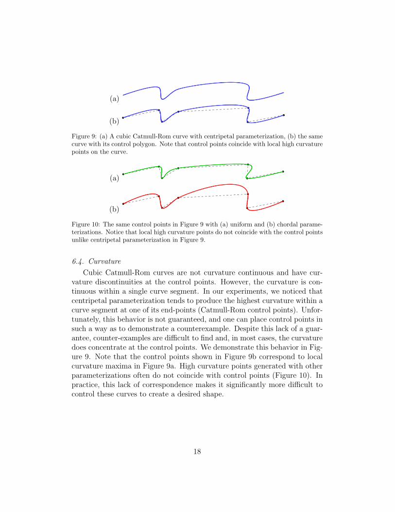
Figure 9: (a) A cubic Catmull-Rom curve with centripetal parameterization, (b) the samecurve with its control polygon. Note that control points coincide with local high curvaturepoints on the curve.

(a)

(b)

Figure 10: The same control points in Figure 9 with (a) uniform and (b) chordal parame-terizations. Notice that local high curvature points do not coincide with the control pointsunlike centripetal parameterization in Figure 9.

6.4. Curvature

Cubic Catmull-Rom curves are not curvature continuous and have cur-vature discontinuities at the control points. However, the curvature is con-tinuous within a single curve segment. In our experiments, we noticed thatcentripetal parameterization tends to produce the highest curvature within acurve segment at one of its end-points (Catmull-Rom control points). Unfor-tunately, this behavior is not guaranteed, and one can place control points insuch a way as to demonstrate a counterexample. Despite this lack of a guar-antee, counter-examples are difficult to find and, in most cases, the curvaturedoes concentrate at the control points. We demonstrate this behavior in Fig-ure 9. Note that the control points shown in Figure 9b correspond to localcurvature maxima in Figure 9a. High curvature points generated with otherparameterizations often do not coincide with control points (Figure 10). Inpractice, this lack of correspondence makes it significantly more difficult tocontrol these curves to create a desired shape.

18

7. Applications

Catmull-Rom curves have a wide range of applications, particularly thoseinvolving interpolation of control points. The fact that they have local sup-port and that they have a polynomial representation also make Catmull-Romcurves preferable over other curve formulations in many settings. In this sec-tion we discuss two application domains for Catmull-Rom curves and presenthow the choice of parameterization makes a significant difference in those ap-plications.

7.1. Animation Curves

There are several applications, ranging from robotics to computer anima-tion, in which a set of parameters x need to be interpolated over time. Theparameters may be joint angles, positions, or even higher order terms suchas velocity. These parameters are specified at particular points in time, andit is crucial to have a smooth interpolation of these values. We will referto these interpolations, generally, as animation curves. Borrowing the lan-guage of computer animation, we will refer to the parameters as animationparameters, and a specific specification of parameters to be interpolated at aparticular time as a key-frame. Catmull-Rom curves are already popular forcreating animation curves, but they may produce highly undesirable resultsif the parameterization is not chosen properly.

An animation curve is a function x = F (t), which produces a set of anima-tion parameters x at the given time t. We define a Catmull-Rom spline C(s)to represent the curve F (t) where our curve has control points Pi = (ti, xi)defined by the value xi at time ti for the ith key-frame. However, when itcomes to the parameterization of the Catmull-Rom curve, we cannot simplyuse the Euclidean distance between control points Pi, because x and t ingeneral have different units. Since the Euclidean distance that combines twounrelated units is not a meaningful measure, we use the distances betweenkey-frame times ti and ignore the values xi for parameterization.

In this notation the Catmull-Rom curve C(s) can be written as twocurves, such that x = X(s) and t = T (s). Since we only use ti valuesfor building the parameterization si for each key-frame point, in effect theparameterization is computed for T (s) only and the same parameterizationis used for X(s). Using this notation,

F (t) = X(T−1(t)

). (9)

19

x

. t

Figure 11: Chordal (α = 1) and centripetal (α = 12 ) Catmull-Rom curves that interpolate

the same key-frames. The two close-by key-frames in the middle cause the chordal curveto overshoot and highly deviate from the control polygon, while the centripetal curvedeviates significantly less. The shaded segments of these curves are used for driving theanimation in Figure 12.

Notice that for T (s) to have an inverse, t = T (s) must be one-to-one andonto over the time range of the animation. In effect (since this is a curvein one dimension), we want T (s) to be monotonic. Notice that if T (s) isnot monotonic, then the results would be meaningless in terms of animation,since there would essentially be two or more values of x for a given value oft. We ensure that T (s) meets this criterion by ensuring that the Catmull-Rom curve we use for representing T (s) does not have self-intersections. Weknow that for general Catmull-Rom curves, only centripetal parameterizationguarantees no self-intersections within a curve segment. However, animationcurves are a special case, because each ti has to be strictly increasing (i.e.ti < ti+1). We therefore examine this case in more detail.

For monotonically increasing ti, cos(θ) = −1 in Equation 3 and so Equa-tion 3 can never be satisfied regardless of the value of α. Hence, the curveT (s) cannot have a negative derivative at its end-points (if the derivative werenegative, the curve could not be monotonically increasing). However, T (s)may have an interior cusp if the curve does not meet Theorem 2. Unfortu-nately, for α ∈ [0, 1

2), Equation 4 may be satisfied and an interior cusp may

exist, meaning that T (s) is not invertible. This fact implies that buildingsuch animation curves with α < 1

2is not possible in general.

Nevertheless, for α ∈ [12, 1], monotonic ti imply that a monotonic curve

T (s) and T−1(t) will always exist. Moreover, since T (s) is monotonic andinterpolates the ti, finding T−1(t) can be performed via a simple bisectionover the parameter interval ti ≤ t ≤ ti+1. Finally, for the special case ofchordal parameterization (α = 1), t = T (s) = s since Catmull-Rom curveshave linear precision and the inverse simplifies in Equation 9.

We are then left with the question of whether any particular parameter-

20

Figure 12: Animation of a robot arm comparing the interpolation generated by chordal(α = 1) and centripetal (α = 1

2 ) Catmull-Rom curves. The first and the last two framesare key-frames and the rest are interpolated. This animation corresponds to the shadedsegment of the animation curves in Figure 11. Notice that the interpolation with chordalparameterization highly deviates from user defined key-frame poses.

izations in the range α ∈ [12, 1] are better than others. In our experiments

with animation curves using various values of α we observed that as α getslarger, the resulting Catmull-Rom curve deviates further away from the con-trol polygon of the curve (the straight lines that connect consecutive controlpoints) for segments that interpolate distant key-frames. This is equivalentto saying that the interpolated animation will deviate more from the user-defined key-frame values. This observation is consistent with our discussionsin the previous sections. As the α value gets closer to 1, the resulting anima-tion curve becomes more sensitive to the direction of control polygon edgesthat are shorter than their neighbors. That is, closely-placed key frames

21

will tend to have a greater impact (creating more deviation) on interpolatedframes farther from the key-frames.

Figure 11 demonstrates this effect by showing animation curves that in-terpolate a set of key-frame values using Catmull-Rom curves with α = 1

2

and α = 1. As can be seen from this figure, chordal parameterization (α = 1)produces curves that deviate further when interpolating distant key-frames.We also used a segment of these curves to derive an animation of a robot arm,shown in Figure 12. The interpolated frames in Figure 12 show how muchmore exaggerated the motion is with chordal parameterization as comparedto centripetal parameterization.

7.2. Path Curves

Another possible application for Catmull-Rom splines are path curvesthat define the motion path of an object in 3D space. These curves can arisein multiple domains where the position/configuration of a device is specifiedat certain points. For example, in robotics, probabilistic roadmaps [11] repre-sent a path as connected points along a graph, but the paths are typically notsmooth. Catmull-Rom splines provide a simple method for creating smoothcurves that follow the discovered path. Likewise, tool path generation mayrequire a smooth path that interpolates various 3D points on a machinedsurface; Catmull-Rom splines can provide such a curve.

Just like animation curves, path curves are also defined by a number ofkey-frame positions and the curve must interpolate these key-frame points.Unlike animation curves, however, path curves do not specify time values andgeometrically simply represent a curve in the space of animation parametersx.

Loops and self-intersecting curve segments are often undesirable pathcurves. Moreover, key-frames are generally used for representing the extremepositions of a motion. Therefore, it is preferable that the curve does not over-shoot the key-frames. As we have shown, only centripetal parameterizationof Catmull-Rom curves guarantees these conditions.

When centripetal parameterization is used with Catmull-Rom splines todefine a path curve, the direction of motion for the object following this pathwill always be towards the next key-frame position. Let P1 and P2 be thetwo consecutive key-frame positions that a curve segment interpolates. Thesegment of the Catmull-Rom curve between P1 and P2 is guaranteed to be inthe same direction as the line connecting P1 and P2 (the dot product of thederivative of the curve and P2 − P1 will be positive) when using centripetal

22

parameterization. Therefore, the object always moves from one control pointtowards the next one and never in the opposite direction.

Note that when using Catmull-Rom splines for representing path curves,these curves only represent the shape of the path and do not provide a posi-tions for a given time t like animation curves do. Instead, these curves focusmore on the shape of the curve. To provide a desired speed along the curve,we typically must reparameterize the curve. The natural parameterizationof the curve provided by s will produce a wide range of speeds along thecurve for different values of the parameterization constant α. The desiredreparameterization of the curve may not have an analytical solution (for ex-ample arc-length parameterization); however, most reparameterizations canbe easily computed numerically.

8. Conclusion

Our analysis on the parameterization of cubic Catmull-Rom curvesdemonstrates that centripetal parameterization has special properties. Inparticular, this parameterization was the only parameterization that guaran-teed no local self-intersections of the curve. Furthermore, we created distancebounds of the curve to its control polygon for curves within this parameteriza-tion family. Using these distance bounds, we derived angle constraints on thecontrol polygon that could guarantee Catmull-Rom curves with centripetalparameterization were globally intersection free. Finally, these propertieswere valid in general dimension Rm.

Currently, we have only explored C1 Catmull-Rom curves. While thesecurves are by far the most popular in the family of Catmull-Rom curves, wehave yet to examine higher degree curves. One important property that is lostwith higher degree Catmull-Rom curves is the lack of local self-intersectionswith centripetal parameterization as we can create cases where this phe-nomenon happens even using C2 Catmull-Rom curves. However, the fre-quency of such self-intersection seems to be less than with other parameter-izations, but it is unclear whether anything precise can be said about thisproperty when using higher order continuity.

9. Acknowledgments

This work was funded in part by NSF grant CCF-07024099.

23

References

[1] N. Dyn, M. S. Floater, K. Hormann, Four-point curve subdivision basedon iterated chordal and centripetal parameterizations, Computer AidedGeometric Design 26 (3) (2009) 279–286.

[2] M. P. Epstein, On the influence of parametrization in parametric inter-polation, SIAM Journal on Numerical Analysis 13 (2) (1976) 261–268.

[3] M. S. Floater, T. Surazhsky, Parameterization for curve interpolation,in: Topics in multivariate approximation and interpolation, 2006, pp.39–54.

[4] E. T. Y. Lee, Choosing nodes in parametric curve interpolation, Com-puter Aided Design 21 (6) (1989) 363–370.

[5] M. S. Floater, On the deviation of a parametric cubic spline interpolantfrom its data polygon, Computer Aided Geometric Design 25 (3) (2008)148–156.

[6] E. Catmull, R. Rom, A class of local interpolating splines, ComputerAided Geometric Design (1974) 317–326.

[7] P. J. Barry, R. N. Goldman, A recursive evaluation algorithm for a classof catmull-rom splines, SIGGRAPH Computer Graphics 22 (4) (1988)199–204.

[8] T. A. Foley, G. M. Nielson, Knot selection for parametric spline inter-polation (1989) 261–272.

[9] G. Nielson, T. Foley, A survey of applications of an affine invariantmetric (1989) 445–468.

[10] D. Manocha, J. F. Canny, Detecting cusps and inflection points incurves, Computer Aided Geometric Design 9 (1) (1992) 1–24.

[11] L. E. Kavraki, P. Svestka, J.-C. Latombe, M. Overmars, Probabilisticroadmaps for path planning in high dimensional configuration spaces,IEEE Transactions on Robotics and Automation 12 (4) (1996) 566–580.

24