Parameter Sensitivity and Boundedness ofRobotic Hybrid Periodic Orbits ?

Shishir Kolathaya ∗ Aaron D. Ames ∗

∗ Georgia Institute of Technology, Atlanta, GA 30332 USA(e-mail: shishirny, ames@gatech.edu).

Abstract: Model-based nonlinear controllers like feedback linearization and control Lyapunovfunctions are highly sensitive to the model parameters of the robot. This paper addresses theproblem of realizing these controllers in a particular class of hybrid models–systems with impulseeffects–through a parameter sensitivity measure. This measure quantifies the sensitivity of agiven model-based controller to parameter uncertainty along a particular trajectory. By usingthis measure, output boundedness of the controller (computed torque+PD) will be analyzed.Given outputs that characterize the control objectives, i.e., the goal is to drive these outputsto zero, we consider Lyapunov functions obtained from these outputs. The main result of thispaper establishes the ultimate boundedness of the output dynamics in terms of this measurevia these Lyapunov functions under the assumption of stable hybrid zero dynamics. This isdemonstrated in simulation on a 5-DOF underactuated bipedal robot.

Keywords: Hybrid Zero Dynamics, Parameter Sensitivity Measure, System Identification.

1. INTRODUCTION

Model based controllers like stochastic controllers Byl andTedrake (2009), feedback linearization Westervelt et al.(2007), the control Lyapunov functions (CLFs) Ames et al.(2014) all require the knowledge of an accurate dynamicalmodel of the system. The advantage of these methods arethat they yield sufficient convergence for highly dynamicrobotic applications, e.g., quadrotors and bipedal robots,where exponential convergence of control objectives is usedto achieve guaranteed stability of the system. This isespecially true of bipedal walking robots where rapid expo-nential convergence is used Ames et al. (2014). While thesecontrollers have yielded good results when an accuratedynamical model is known, there is a need for quantifyinghow accurate the model has to be to realize the desiredtracking error bounds. These application domains point tothe need for a way to measure parameter uncertainty anda methodology to design controllers for nonlinear hybridsystems, like bipedal robots, that can converge to thecontrol objective under parameter uncertainty.

The goal of this paper is to establish a relationship betweenparameter uncertainty and the output error bounds onsystems with alternating continuous and discrete events,i.e., hybrid systems, while considering a specific exam-ple: bipedal walking robots. Inspired by the sensitivityfunctions utilized for linear systems Zhou et al. (1996),a parameter sensitivity measure is defined for continuoussystems and the relationship between the boundednessand the measure is established through the use of Lya-punov functions. In the context of hybrid systems, alongwith defining the measure for the continuous event, animpact measure is defined to include the effect of param-

? This work is supported by the National Science Foundationthrough grants CNS-0953823 and CNS-1136104.

z

x

èsf

èsh

ènsh

èsk

ènsk

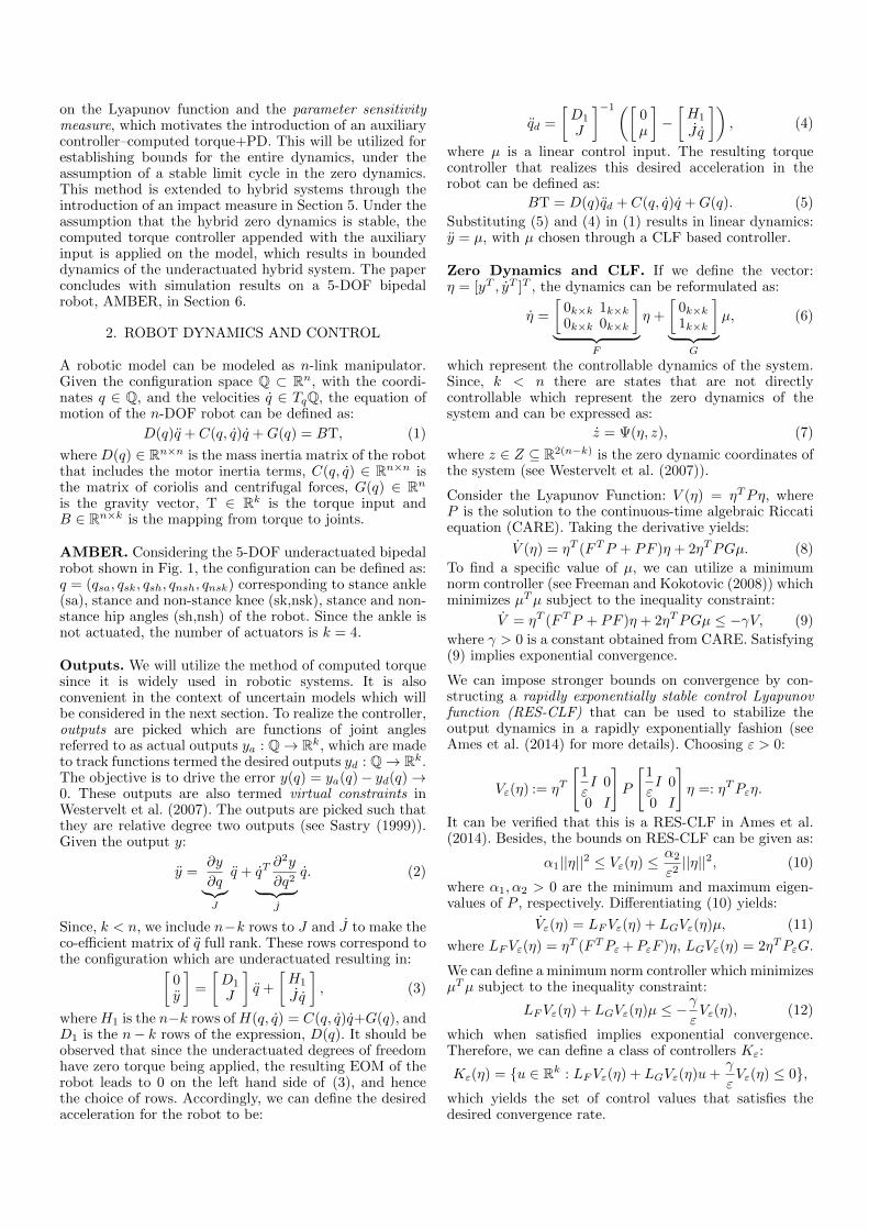
Fig. 1. The biped AMBER (left) and the stick figure ofAMBER showing the configuration angles (right).

eter variations in the discrete event. The resulting overallsensitivity measure thus represents how sensitive a givencontroller is to parameter variations for hybrid systems.When described in terms of Lyapunov functions, whichare constructed from the zeroing outputs of the robot, theparameter sensitivity measure naturally yields the ultimatebound on the outputs. Considering a 5-DOF bipedal robot,AMBER, shown in Fig. 1, where a stable periodic orbit onthe hybrid zero dynamics translates to a stable walkinggait on the bipedal robot, the ultimate bound on thisperiodic orbit will be determined through the use of aparticular controller: computed torque+PD.

The paper is structured in the following fashion: Section 2introduces the robot model and the control methodologyused–CLFs through the method of computed torque. Sec-tion 3 assesses the controller used for the uncertain modelof the robot and establishes the resulting uncertain behav-ior through Lyapunov functions. In Section 4, the resultinguncertain dynamics exhibited by the robot is measuredformally through the construction of parameter sensitivitymeasure, which is the main formulation of this paper onwhich the formal results will build. It will be shown thatthere is a direct relationship between the ultimate bound

on the Lyapunov function and the parameter sensitivitymeasure, which motivates the introduction of an auxiliarycontroller–computed torque+PD. This will be utilized forestablishing bounds for the entire dynamics, under theassumption of a stable limit cycle in the zero dynamics.This method is extended to hybrid systems through theintroduction of an impact measure in Section 5. Under theassumption that the hybrid zero dynamics is stable, thecomputed torque controller appended with the auxiliaryinput is applied on the model, which results in boundeddynamics of the underactuated hybrid system. The paperconcludes with simulation results on a 5-DOF bipedalrobot, AMBER, in Section 6.

2. ROBOT DYNAMICS AND CONTROL

A robotic model can be modeled as n-link manipulator.Given the configuration space Q ⊂ Rn, with the coordi-nates q ∈ Q, and the velocities q ∈ TqQ, the equation ofmotion of the n-DOF robot can be defined as:

D(q)q + C(q, q)q +G(q) = BT, (1)

where D(q) ∈ Rn×n is the mass inertia matrix of the robotthat includes the motor inertia terms, C(q, q) ∈ Rn×n isthe matrix of coriolis and centrifugal forces, G(q) ∈ Rnis the gravity vector, T ∈ Rk is the torque input andB ∈ Rn×k is the mapping from torque to joints.

AMBER. Considering the 5-DOF underactuated bipedalrobot shown in Fig. 1, the configuration can be defined as:q = (qsa, qsk, qsh, qnsh, qnsk) corresponding to stance ankle(sa), stance and non-stance knee (sk,nsk), stance and non-stance hip angles (sh,nsh) of the robot. Since the ankle isnot actuated, the number of actuators is k = 4.

Outputs. We will utilize the method of computed torquesince it is widely used in robotic systems. It is alsoconvenient in the context of uncertain models which willbe considered in the next section. To realize the controller,outputs are picked which are functions of joint anglesreferred to as actual outputs ya : Q→ Rk, which are madeto track functions termed the desired outputs yd : Q→ Rk.The objective is to drive the error y(q) = ya(q)− yd(q)→0. These outputs are also termed virtual constraints inWestervelt et al. (2007). The outputs are picked such thatthey are relative degree two outputs (see Sastry (1999)).Given the output y:

y =∂y

∂q︸︷︷︸J

q + qT∂2y

∂q2︸ ︷︷ ︸J

q. (2)

Since, k < n, we include n−k rows to J and J to make theco-efficient matrix of q full rank. These rows correspond tothe configuration which are underactuated resulting in:[

0y

]=

[D1

J

]q +

[H1

J q

], (3)

where H1 is the n−k rows of H(q, q) = C(q, q)q+G(q), andD1 is the n− k rows of the expression, D(q). It should beobserved that since the underactuated degrees of freedomhave zero torque being applied, the resulting EOM of therobot leads to 0 on the left hand side of (3), and hencethe choice of rows. Accordingly, we can define the desiredacceleration for the robot to be:

qd =

[D1

J

]−1([0µ

]−[H1

J q

]), (4)

where µ is a linear control input. The resulting torquecontroller that realizes this desired acceleration in therobot can be defined as:

BT = D(q)qd + C(q, q)q +G(q). (5)

Substituting (5) and (4) in (1) results in linear dynamics:y = µ, with µ chosen through a CLF based controller.

Zero Dynamics and CLF. If we define the vector:η = [yT , yT ]T , the dynamics can be reformulated as:

η =

[0k×k 1k×k0k×k 0k×k

]︸ ︷︷ ︸

F

η +

[0k×k1k×k

]︸ ︷︷ ︸

G

µ, (6)

which represent the controllable dynamics of the system.Since, k < n there are states that are not directlycontrollable which represent the zero dynamics of thesystem and can be expressed as:

z = Ψ(η, z), (7)

where z ∈ Z ⊆ R2(n−k) is the zero dynamic coordinates ofthe system (see Westervelt et al. (2007)).

Consider the Lyapunov Function: V (η) = ηTPη, whereP is the solution to the continuous-time algebraic Riccatiequation (CARE). Taking the derivative yields:

V (η) = ηT (FTP + PF )η + 2ηTPGµ. (8)

To find a specific value of µ, we can utilize a minimumnorm controller (see Freeman and Kokotovic (2008)) whichminimizes µTµ subject to the inequality constraint:

V = ηT (FTP + PF )η + 2ηTPGµ ≤ −γV, (9)

where γ > 0 is a constant obtained from CARE. Satisfying(9) implies exponential convergence.

We can impose stronger bounds on convergence by con-structing a rapidly exponentially stable control Lyapunovfunction (RES-CLF) that can be used to stabilize theoutput dynamics in a rapidly exponentially fashion (seeAmes et al. (2014) for more details). Choosing ε > 0:

Vε(η) := ηT

[1

εI 0

0 I

]P

[1

εI 0

0 I

]η =: ηTPεη.

It can be verified that this is a RES-CLF in Ames et al.(2014). Besides, the bounds on RES-CLF can be given as:

α1||η||2 ≤ Vε(η) ≤ α2

ε2||η||2, (10)

where α1, α2 > 0 are the minimum and maximum eigen-values of P , respectively. Differentiating (10) yields:

Vε(η) = LFVε(η) + LGVε(η)µ, (11)

where LFVε(η) = ηT (FTPε +PεF )η, LGVε(η) = 2ηTPεG.

We can define a minimum norm controller which minimizesµTµ subject to the inequality constraint:

LFVε(η) + LGVε(η)µ ≤ −γεVε(η), (12)

which when satisfied implies exponential convergence.Therefore, we can define a class of controllers Kε:

Kε(η) = {u ∈ Rk : LFVε(η) + LGVε(η)u+γ

εVε(η) ≤ 0},

which yields the set of control values that satisfies thedesired convergence rate.

3. UNMODELED DYNAMICS

Since the parameters are not perfectly known, the equationof motion, (1), computed with the given set of parameterswill henceforth haveˆover the symbols. Therefore, Da, Ca,Ga represent the actual model of the robot, and D, C, Grepresent the assumed model of the robot.

It is a well known fact that the inertial parameters of arobot are affine in the EOM (see Spong et al. (2006)).Therefore (1) can be restated as:

Y(q, q, q)Θ = BT, (13)

where Y(q, q, q) is the regressor Spong et al. (2006), andΘ is the set of base inertial parameters. Accordingly, Θa

and Θ are the actual and the assumed set of base inertialparameters respectively.

Computed Torque Redefined. The method of com-puted torque becomes very convenient to apply if theregressor and the inertial parameters are being computedsimultaneously. If qd is the desired acceleration for therobot, the method of computed torque can be defined as:

BTct = Y(q, q, qd)Θ. (14)

For convenience, the mapping matrix B on the left handside of (14) will be omitted i.e., BTct = Tct. Due to thedifference in parameters, the dynamics will deviate fromthe nominal model, which is shown below:

Lemma 1. Define:

Φ = D−1Y(q, q, q), (15)

which is a function of the estimated parameters, Θ. If thecontrol law used is (4) combined with the computed torque(14), then the resulting dynamics of the robot evolve as:

y = µ+ JΦ(Θ−Θa). (16)

Described in terms of η, we have the following:

η = Fη +Gµ+GJΦΘ, z = Ψ(η, z), (17)

where Θ = Θ−Θa. If Θ = 0, we could apply µ(η) ∈ Kε(η)to drive η → 0. But since the parameters are uncertain,i.e., Θ 6= 0, the resulting dynamics will be observed in thederivative of the Lyapunov function, Vε, via

Vε(η, µ) = ηT (FTPε + PεF )η + 2ηTPεGµ (18)

+ 2ηTPεGJΦΘ,

where η is obtained via (17). The next section will establishthe relationship between parameter uncertainty and theuncertain dynamics appearing in the CLF.

4. PARAMETER SENSITIVITY MEASURE

Due to the unmodeled dynamics, applying the controller,µ(η) ∈ Kε(η), does not result in exponential convergenceof the controller. The controller will still yield GlobalUniform Ultimate Boundedness (GUUB) based on how the

unmodeled dynamics affect Vε. The parameter sensitivitymeasure, ν, that quantifies the ultimate bound on theLyapunov function Vε is defined as:

ν := Y(q, q, q)Θ. (19)

It can be observed that: Y(q, q, q)Θ = Y(q, q, q)Θ −Y(q, q, q)Θa, which is the difference between the actual

and the expected torque being applied on the robot.Therefore, the parameter sensitivity measure is effectivelythe difference in torques applied on the robot.

Bounds on the Measure through RES-CLF. By (15)

and (19), we have: D−1ν = ΦΘ. Therefore, (18) can beexpressed as:

Vε(η, µ) =ηT (FTPε + PεF )η + 2ηTPεGµ

+ 2ηTPεGJD−1ν, (20)

which is now a function of ν. This provides an impor-tant connection with Lyapunov theory, and the notion ofparameter sensitivity is motivated by this observation. Inother words, if the path of least parameter sensitivity isfollowed, then the convergence of the Lyapunov functionto a value very close to zero can be realized. Therefore by(20), the control input µ must be chosen such that ν iswell within the bounds specified. If a suitable controlleris applied: µ(η) ∈ Kε(η) , the stability of the Lyapunovfunction can be achieved as long as the following equationis satisfied:

Vε ≤ −γ

εVε + 2ηTPεGJD

−1ν ≤ 0, (21)

Since the measure ν is a function of the control input µ,(21) has an algebraic loop. But, given the control input,it is possible to restrict the outputs η within a certainregion. Therefore, we first assume the bounds on theinertia matrix as:

α3 ≤ ||D|| ≤ α4, α3 ≤ ||D|| ≤ α4, (22)

where α3, α4, α3, α4 are constants (see Mulero-Martinez(2007); From et al. (2010)). Since the outputs are degreeone functions of q, the jacobian is bounded by the constant:||J || ≤ κ.

By varying γ, it can be shown that the controller exponen-tially drives the outputs to a ball of radius β. In particular,by considering γ1 > 0, γ2 > 0, which satisfy γ = γ1+γ2, wecan rewrite γ

εVε = γ1ε Vε + γ2

ε Vε in (21). The first term canthus be used to cancel the uncertain dynamics and yieldexponential convergence until ||η|| becomes sufficientlysmall. In other words, the outputs exponentially convergeto an ultimate bound β as given by the following lemma.

Lemma 2. Given the controllers µ(η) ∈ Kε(η), µ(η) ∈Kε(η), and δ > 0, ∃ β > 0 such that whenever ||ν|| ≤ δ,

Vε(η) < −γ2ε Vε(η) ∀ Vε(η) > β.

The ultimate bound is given by β =4α2

2κ2δ2

α1α23γ

21ε

2 . A discussion

in this regard can be found in Dixon et al. (2004); Abdallahet al. (1991), where β is considered the uniform ultimatebound on the given controller.

It must be noted that Lemma 2 yields a low convergencerate γ2 which is less than the original rate γ. The uncertaindynamics can be nullified separately by considering anauxiliary input µ satisfying:

BTctn = D(q)qd + C(q, q)q + G(q) +Bµ. (23)

Note that this is not unique and other types of controllerscan also be used. Computed torque with linear inputsappended have also been used in Slotine and Li (1987)in order to realize asymptotic convergence. The resultingdynamics of the outputs then reduces to:

y = µ+ JΦΘ + JD−1Bµ. (24)

Therefore, Vε for the new input can be reformulated as:

Vε(η, µ, µ) = ηT (FTPε + PεF )η + 2ηTPεGµ (25)

+ 2ηTPεGJD−1(ν +Bµ).

Consider the input µ = − 1εΓTGTPεη, where Γ = JD−1B.

µ and µ together form the computed torque+PD controlon the robot. The end result is a positive semidefiniteexpression: 1

εηTPεGΓΓTGTPεη ≥ 0, which motives the

construction of a positive semidefinite function:

Vε(η) = ηTPεGΓΓTGTPεη =: ηT Pεη. (26)

Using the property of positive semidefiniteness, we canestablish new bounds on the outputs. Let N (Pε) be thenull space of the matrix Pε. If η ∈ N (Pε), then Vε(η) = 0.Otherwise, for some α7, α8 > 0:

α7||η||2 ≤ Vε(η) ≤ α8

ε4||η||2. (27)

Note that (27) can be used to restrict the uncertaindynamics in (25). Utilizing these constructions, we candefine the following class of controllers:

Kε(η) = {u ∈ Rk : 2ηTPεGJD−1Bu+

1

εVε(η) ≤ 0},

Lemma 2 can now be redefined to obtain the new ultimatebound βη for the new control input (23).

Lemma 3. Given the controllers µ(η) ∈ Kε(η), µ(η) ∈Kε(η), and δ > 0, ∃ βη > 0 such that whenever ||ν|| ≤ δ,

Vε(η) < −γεVε(η) ∀ Vε(η) > βη.

The resulting ultimate bound is: βη =4α2

2κ2δ2ε2

α7α29α

23ε

4 , where

α9 = VεVε

. It can be inferred that:

Vε(η(t)) ≤ e−γε tVε(η(0)) for Vε(η(0)) > βη, (28)

or ||η(t)|| ≤ 1

ε

√α2

α1e−

γ2ε t||η(0)|| for Vε(η(0)) > βη.

It must be noted that both ε, ε affect ||ν||. We can nowconsider utlizing the boundedness properties in underac-tuated systems given that the zero dynamics of the robothas a locally exponentially stable periodic orbit.

Zero Dynamics. Assume that there is an exponentiallystable periodic orbit in the zero dynamics, denoted byOz ⊂ Z. This means that there is a Lyapunov functionVz : Z → R≥0 such that in a neighborhood Br(Oz) of Oz(see Hauser and Chung (1994)) it is exponentially stable.If O = ι(Oz) ⊂ X×Z is the periodic orbit of the full orderdynamics through the canonical embedding ι : Z → X×Z,then by defining the composite Lyapunov function:

Vc(η, z) = σVε(η) + Vz(z), (29)

we can introduce a theorem that shows ultimate bound-edness of the entire dynamics of the robot to the periodicorbit O under parameter uncertainty.

Theorem 1. Given the controllers µ(η) ∈ Kε(η), µ(η) ∈Kε(η), and δ > 0, ∃ βη, βz > 0 such that whenever ||ν|| ≤δ, Vc(η, z) is exponentially convergent ∀ Vc(η, z) > βη+βz.

Proof of Theorem 1 is omitted due to space constraintsbut is an extension of Theorem 1 of Ames et al. (2014)which shows that by choosing a suitable σ, exponentialconvergence of Vc until the bound βη+βz can be achieved.

5. HYBRID DYNAMICS

We now extend Theorem 1 to hybrid robotic systemswhich involve alternating phases of continuous and discretedynamics. A hybrid system with a single continuous anda discrete event is defined as follows:

H =

η = Fη +Gµ+GJΦΘ,z = Ψ(Θ; η, z), if (η, z) ∈ D\Sη+ = ∆η(Θ, η−, z−),z+ = ∆z(Θ, η

−, z−), if (η−, z−) ∈ S

(30)

It must be noted that the parameter vector Θ is includedin zero dynamics, z, in (30), which is a reformulation of(7). D,S are the domain and switching surfaces and aregiven by:

D = {(η, z) ∈ X × Z : h(η, z) ≥ 0}, (31)

S = {(η, z) ∈ X × Z : h(η, z) = 0 and h(η, z) < 0},for some continuously differentiable function h : X ×Z → R. ∆(Θ, η−, z−) = (∆η(Θ, η−, z−),∆z(Θ, η

−, z−))is the reset map representing the discrete dynamics ofthe system. For the bipedal robot, AMBER, h representsthe non-stance foot height and ∆ represents the impactdynamics of the system. Plastic impacts are assumed. For(q−, q−) ∈ S, being the pre-impact angles and velocities ofthe robot, the post impact velocity for the assumed model˙q+, and for the actual model q+ will be:

˙q+ = (I − D−1J T (J D−1J T )−1J )q−,

q+ = D−1a (D − J TRD) ˙q+ − (I − J TR)Dq−, (32)

where J is the jacobian of the end effector where theimpulse forces from the ground are acting on the robot,and R = (JD−1

a J T )−1JD−1a . Given the hybrid system

(30), denote the flow as ϕt(Θ; ∆(Θ, η−, z−)) with theinitial condition (η−, z−) ∈ S ∩ Z.

Impact Measure. Using the impact model, measuringuncertainty of post-impact dynamics can be achieved byintroducing an impact measure, νs, defined as follows:

νs := D(q)q−, (33)

It should be noted that the impact equations are Lipschitzcontinuous w.r.t. the impact measure νs. Accordingly, wehave the following bounds on the impact map:

||∆η(Θa, η−, z−)−∆η(Θ, 0, z−)||≤ ||∆η(Θa, η

−, z−)−∆η(Θ, η−, z−)

+ ∆η(Θ, η−, z−)−∆η(Θ, 0, z−)||≤ L1||νs||+ L2||η−||, (34)

where L1, L2 are Lipschitz constants for ∆η. Similarly:

||∆z(Θa, η−, z−)−∆z(Θ, 0, z

−)|| ≤ L3||νs||+ L4||η−||,where L3, L4 are Lipschitz constants for ∆z. In order toobtain bounds on the output dynamics for hybrid periodicorbits, it is assumed that H has a hybrid zero dynamicsfor the assumed model, Θ, of the robot. The hybrid zerodynamics can be described as:

H |Z =

{z = Ψ(Θ; 0, z) if z ∈ Z\(S ∩ Z)

z+ = ∆Z(Θ, 0, z−) if z− ∈ (S ∩ Z)(35)

More specifically we assume that ∆η(Θ; 0, z−) = 0, so thatthe surface Z is invariant under the discrete dynamics.Given (35), we can define the flow as ϕzt (Θ; ∆(Θ, 0, z−))

with the initial state (0, z−) ∈ S ∩ Z. If a periodicorbit Oz exists in (35), then there exists a periodic

flow ϕzt (Θ; ∆(Θ, 0, z∗)) of period T ∗ for the fixed point(0, z∗). Through the canonical embedding, the correspond-ing periodic flow of the periodic orbit O in (30) will be

ϕt(Θ; ∆(Θ, 0, z∗)). Note that existence of periodic orbit

for the assumed model Θ does not guarantee existence ofthe periodic orbit for the actual model Θa. Therefore, wedefine the Poincare map P : S→ S given by:

P(Θ; η, z) = ϕT (Θ,η,z)(Θ; ∆(Θ, η, z)), (36)

where Θ can be either Θa or Θ, and T is the time to impactfunction defined by:

T (Θ; η, z) = inf{t ≥ 0 : ϕt(Θ; ∆(Θ, η, z)) ∈ S}. (37)

It is shown in Ames et al. (2014) that T is Lipschitzcontinuous. Therefore, for constants α15 < 1 < α16,α15T

∗ ≤ T (Θ, η, z) ≤ α16T∗. These constants depend on

the deviation from the nominal model Θ and how far (η, z)is from the fixed point. The corresponding Poincare mapρ : S ∩ Z → S ∩ Z for the hybrid zero dynamics (35) istermed the restricted Poincare map:

ρ(z) = ϕzTρ(z)(Θ; ∆(Θ, 0, z)), (38)

where Tρ is the restricted time to impact function which

is given by Tρ(z) = T (Θ; 0, z). Without loss of generality,

we can assume that Θ = 0, z∗ = 0. The following Lemmawill introduce the relationship between time to impact,Poincare functions with η, νs.

Lemma 4. Let Oz be the periodic orbit of the hybrid zerodynamics H |Z transverse to S∩Z for the nominal model

Θ. Given the controllers µ(η) ∈ Kε(η), µ(η) ∈ Kε(η) forthe actual model Θa which render ultimate boundedness onVε(η), (η, z) ∈ S∩Z such that Vε(∆η(Θ, η, z)) > βη for thegiven robot model Θ, and r > 0 such that (η, z) ∈ Br(0, 0),there exist finite constants A1, A2, A3, A4 > 0 such that:

||T (Θa; η, z)− Tρ(z)|| ≤ A1||η||+A2||νs|| (39)

||P(Θa; η, z)− ρ(z)|| ≤ A3||η||+A4||νs|| (40)

Proof (Sketch). Let µ1 ∈ R2(n−k), µ2 ∈ R2k be constantvectors. Define an auxiliary time to impact function:TB(µ1, µ2, z) = inf{t ≥ 0 : h(µ1, ϕ

zt (0,∆(0, 0, z)) +

µ2) = 0}, which is Lipschitz continuous with the Lipschitzconstant LB : ||TB(µ1, µ2, z)−Tρ(z)|| ≤ LB(||µ1||+ ||µ2||).Let (η1(t), z1(t)) satisfy z1 = Ψ(Θa; η1(t), z1(t)) withη1(0) = ∆η(Θa, η, z) and z1(0) = ∆z(Θa, η, z). Similarlylet z2(t) satisfy z2(t) = Ψ(0; 0, z2(t)) such that z2(0) =∆z(0, 0, z). The bounds on the ||η|| can now be given as||η1(0)|| = ||∆η(Θ, η, z)−∆η(0, 0, z)|| ≤ L1||νs||+ L2||η||,which is obtained through (34). Since Vε(η1) > βη, we use(59) of Lemma 1 of Ames et al. (2014) and (28) to obtain||µ1||. Similartly, to obtain ||µ2||, we use the Gronwall-Bellman argument from the proof of Lemma 1 of Ameset al. (2014) to get the following inequality:

||z1(t)− z2(t)|| ≤ (C2||η||+ C3||νs||) eLqt, (41)

where C2, C3, Lq are constants. Proof of (39) can now beobtained by substituting for ||µ1||, ||µ2||.Similarly, the derivation of (54) of Lemma 1 of Ames et al.(2014) is used to obtain (40).

Main Theorem. We can now introduce the main theoremof the paper. Similar to the continuous dynamics, it isassumed that the periodic orbit OZ is exponentially stablein the hybrid zero dynamics.

Theorem 2. Let Oz be an exponentially stable periodicorbit of the hybrid zero dynamics H |Z transverse to S∩Zfor the nominal model Θ. Given the controllers µ(η) ∈Kε(η), µ(η) ∈ Kε(η) for the hybrid system H . Given r >0 such that (η, z) ∈ Br(0, 0), there exist δ > 0, δs > 0 suchthat whevener ||ν|| < δ,||νs|| < δs, the orbit O = ι(OZ) isuniformly ultimately bounded by βη + βz.

Proof (Sketch). Results of Lemma 4 and the exponentialstability of OZ imply that there exists r > 0 such thatρ : Br(0) ∩ (S ∩ Z) → Br(0) ∩ (S ∩ Z) is well definedfor all z ∈ Br(0) ∩ (S ∩ Z) and zk+1 = ρ(zk) is locallyexponentially stable, i.e., ||zk|| ≤ Nξk||z0|| for some N >0, 0 < ξ < 1 and all k ≥ 0. Therefore, by the converseLyapunov theorem for discrete systems, there exists anexponentially convergent Lyapunov function Vρ, definedon Br(0) ∩ (S ∩ Z) for some r > 0 (possibly smaller thanthe previously defined r). It must be first ensured thatthe region βη must be within the bounds defined by r.For ||η|| = r, βη < Vε(η) is ensured through the followingcondition: βη < Vε(η) < α2

ε2 ||η||2 < α2

ε2 r2. From Lemma 2

we have:4α3

2κ2δ2

α21α

23γ

21ε

4 <α2

ε2 r2 =⇒ δ < α1α3γ1ε

2

2α2κr.

For the RES-CLF Vε, denote its restriction to the switch-ing surface by Vε,η = Vε|S , which is exponentially conver-gent. With these two Lyapunov functions we define thefollowing candidate Lyapunov function on Br(0, 0) ∩ S:

VP (η, z) = Vρ(z) + σVε,η(η) (42)

The idea is to show that there exists a bounded region βinto which the dynamics of the robot exponentially con-verge. Since the origin is an exponentially stable equilib-rium for zk+1 = ρ(zk), we have the following inequalities:

||Pz(Θa; η, z)|| = ||Pz(Θa; η, z)− ρ(z) + ρ(z)− ρ(0)||≤ A3||η||+A4||νs||+ Lρ||z||

||ρ(z)|| ≤ Nξ||z||, (43)

where Lρ is the Lipschitz constant for ρ. Therefore:

Vρ(Pz(Θa; η, z))− Vρ(ρ(z)) (44)

≤ α20(A3||η||+A4||νs||)(A3||η||+A4||νs||+ (Lρ +Nξ)||z||),

where α20 is equivalent to the constant r4 given in (61) ofproof of Theorem 2 in Ames et al. (2014). It follows that:

Vρ(Pz(Θa, η, z))− Vρ(z) = Vρ(Pz(Θa; η, z))− Vρ(ρ(z))

+Vρ(ρ(z))− Vρ(z).Combining the entire Lyapunov function we have:

VP (P(Θa; η, z))− VP (η, z) ≤ −

[ ||η||||z||||νs||

]TΛH

[ ||η||||z||||νs||

]where the symmetric matrix ΛH ∈ R3×3, is obtainedby collecting the constant terms. It can found in thederivation of Theorem 2 of Ames et al. (2014) that bychoosing a suitable σ positive definiteness of ΛH can beestablished to render the discrete Lyapunov function VPexponentially convergent. The upper bound on the impactmeasure is obtained by applying the contraint on the aboveequation to ensure exponential convergence.

6. SIMULATION RESULTS AND CONCLUSIONS

In this section, we will invesigate how the uncertainty inparameters affects the stability of the controller applied tothe 5-DOF bipedal robot AMBER shown in Fig. 1. Themodel, Θa, which has 61 parameters is picked such thatthe error is 30% compared to the assumed model Θ.

To realize walking on the robot, the actual and desired out-puts are chosen as in Yadukumar et al. (2012) (specifically,see (6) for determining the actual and the desired outputs).The end result is outputs of the form y(q) = ya(q)− yd(q)which must be driven to zero. Therefore, the objective ofthe computed torque controller (5) combined with Kε for

µ and Kε for µ is to drive y → 0. For the nominal model Θa stable walking gait is observed. In other words, a stablehybrid periodic orbit is observed for the assumed givenmodel. Since, the actual model of the robot has an errorof 30%, applying the controller yields the dynamics thatevolves as shown in (24). The value of ε chosen was 1, andε was 2. Fig. 2 shows the comparison between actual anddesired outputs, and Fig. 3 shows the Lyapunov functionVε. It can be observed that after every impact, Vε is thrownoutside the ball defined by βη ≈ 0.04 and the controllersact to get back into βη before the next impact.

Time(s)0 0.5 1 1.5 2 2.5 3

Stance

knee

0.2

0.25

0.3

0.35

0.4

Time(s)0 0.5 1 1.5 2 2.5 3

Non

-stance

knee

0.3

0.4

0.5

0.6

0.7

0.8

0.9

1

1.1

1.2

Time(s)0 0.5 1 1.5 2 2.5 3

Non

-stance

slop

e

-0.2

-0.1

0

0.1

0.2

Time(s)0 0.5 1 1.5 2 2.5 3

Torso

angle

-0.4

-0.3

-0.2

-0.1

0

0.1

0.2

0.3

0.4

Fig. 2. Actual (blue) and desired (red) outputs as afunction of time are shown here.

0 0.5 1 1.5 2 2.5 3 3.5−0.05

0

0.05

0.1

0.15

0.2

0.25

0.3

Time (s)

CLF(V

ǫ)

Lyapunov Function

0 0.5 1 1.5 2 2.5 30

0.5

1

1.5

2

2.5

Time (s)

Measure

(||ν||)

Fig. 3. The RES-CLF (left) and the measure (right) as

a function of time are shown here. Vε crosses 0 inevery step, but the CLF is still seen to be ultimatelybounded by βη.

Conclusions. The concept of a measure for evaluatingthe robustness to parameter uncertainty of hybrid sys-tem models of robots was introduced. This relationshipis created by introducing the formula for the parameter

sensitivity measure. The notion of measure is extended tohybrid systems (which includes discrete events) by consid-ering the impact measure. This impact measure along withthe sensitivity measure determine the output boundednessof the composite Lyapunov function for hybrid periodicorbits of the robot. This was then verified by realizing astable walking gait on AMBER having a parameter errorof 30%. It is important to observe that while the param-eter sensitivity measure yields the difference between theactual and the predicted torque applied on the robot, theimpact measure yields the impulsive ground reaction forcesacting upon the robot during impacts. Future work willbe devoted to evaluating the formal results of this paperexperimentally.

REFERENCES

Abdallah, C., Dawson, D., Dorato, P., and Jamshidi, M.(1991). Survey of robust control for rigid robots. ControlSystems, IEEE, 11(2), 24–30. doi:10.1109/37.67672.

Ames, A.D., Galloway, K., Sreenath, K., and Grizzle, J.W.(2014). Rapidly exponentially stabilizing control lya-punov functions and hybrid zero dynamics. AutomaticControl, IEEE Transactions on, 59(4), 876–891.

Byl, K. and Tedrake, R. (2009). Metastable walking ma-chines. The International Journal of Robotics Research,28(8), 1040–1064.

Dixon, W.E., Zergeroglu, E., and Dawson, D.M. (2004).Global robust output feedback tracking control of robotmanipulators. Robotica, 22(04), 351–357.

Freeman, R.A. and Kokotovic, P.V. (2008). Robust nonlin-ear control design: state-space and Lyapunov techniques.Springer.

From, P.J., Schjølberg, I., Gravdahl, J.T., Pettersen, K.Y.,and Fossen, T.I. (2010). On the boundedness andskew-symmetric properties of the inertia and coriolismatrices for vehicle-manipulator systems. In IntelligentAutonomous Vehicles, volume 7, 193–198.

Hauser, J. and Chung, C.C. (1994). Converse lyapunovfunctions for exponentially stable periodic orbits. Sys-tems & Control Letters, 23(1), 27–34.

Mulero-Martinez, J. (2007). Uniform bounds of the cori-olis/centripetal matrix of serial robot manipulators.Robotics, IEEE Transactions on, 23(5), 1083–1089. doi:10.1109/TRO.2007.903820.

Sastry, S.S. (1999). Nonlinear Systems: Analysis, Stabilityand Control. Springer, New York.

Slotine, J.J.E. and Li, W. (1987). On the adaptive controlof robot manipulators. The International Journal ofRobotics Research, 6(3), 49–59.

Spong, M.W., Hutchinson, S., and Vidyasagar, M. (2006).Robot modeling and control, volume 3. Wiley New York.

Westervelt, E.R., Grizzle, J.W., Chevallereau, C., Choi,J.H., and Morris, B. (2007). Feedback Control of Dy-namic Bipedal Robot Locomotion. CRC Press, BocaRaton.

Yadukumar, S.N., Pasupuleti, M., and Ames, A.D. (2012).From formal methods to algorithmic implementation ofhuman inspired control on bipedal robots. In TenthInternational Workshop on the Algorithmic Foundationsof Robotics (WAFR). Cambridge, MA.

Zhou, K., Doyle, J.C., Glover, K., et al. (1996). Robust andoptimal control, volume 40. Prentice Hall Upper SaddleRiver, NJ.