SANDIA REPORT SAND2015-2065 Unlimited Release Printed March 2015

Parameter Estimation for Single Diode Models of Photovoltaic Modules Clifford W. Hansen Prepared by Sandia National Laboratories Albuquerque, New Mexico 87185 and Livermore, California 94550 Sandia National Laboratories is a multi-program laboratory managed and operated by Sandia Corporation, a wholly owned subsidiary of Lockheed Martin Corporation, for the U.S. Department of Energy's National Nuclear Security Administration under contract DE-AC04-94AL85000. Approved for public release; further dissemination unlimited.

2

Issued by Sandia National Laboratories, operated for the United States Department of Energy by Sandia Corporation.

NOTICE: This report was prepared as an account of work sponsored by an agency of the

United States Government. Neither the United States Government, nor any agency thereof, nor any of their employees, nor any of their contractors, subcontractors, or their employees, make any warranty, express or implied, or assume any legal liability or responsibility for the accuracy, completeness, or usefulness of any information, apparatus, product, or process disclosed, or represent that its use would not infringe privately owned rights. Reference herein to any specific commercial product, process, or service by trade name, trademark, manufacturer, or otherwise, does not necessarily constitute or imply its endorsement, recommendation, or favoring by the United States Government, any agency thereof, or any of their contractors or subcontractors. The views and opinions expressed herein do not necessarily state or reflect those of the United States Government, any agency thereof, or any of their contractors.

Printed in the United States of America. This report has been reproduced directly from the

best available copy. Available to DOE and DOE contractors from U.S. Department of Energy Office of Scientific and Technical Information P.O. Box 62 Oak Ridge, TN 37831 Telephone: (865) 576-8401 Facsimile: (865) 576-5728 E-Mail: reports@adonis.osti.gov Online ordering: http://www.osti.gov/bridge Available to the public from U.S. Department of Commerce National Technical Information Service 5285 Port Royal Rd. Springfield, VA 22161 Telephone: (800) 553-6847 Facsimile: (703) 605-6900 E-Mail: orders@ntis.fedworld.gov Online order: http://www.ntis.gov/help/ordermethods.asp?loc=7-4-0#online

3

SAND2015-2065 Unlimited Release

Printed March 2015

Parameter Estimation for Single Diode Models of Photovoltaic Modules

Clifford W. Hansen Photovoltaic and Distributed Systems Integration Department

Sandia National Laboratories P.O. Box 5800

Albuquerque, New Mexico 87185-1033

Abstract Many popular models for photovoltaic system performance employ a single diode model to

compute the I-V curve for a module or string of modules at given irradiance and temperature conditions. A single diode model requires a number of parameters to be estimated from measured I-V curves. Many available parameter estimation methods use only short circuit, open circuit and maximum power points for a single I-V curve at standard test conditions together with temperature coefficients determined separately for individual cells. In contrast, module testing frequently records I-V curves over a wide range of irradiance and temperature conditions which, when available, should also be used to parameterize the performance model.

We present a parameter estimation method that makes use of a full range of available I-V curves. We verify the accuracy of the method by recovering known parameter values from simulated I-V curves. We validate the method by estimating model parameters for a module using outdoor test data and predicting the outdoor performance of the module.

4

ACKNOWLEDGMENTS Dr. Katherine Crowley (Washington and Lee University) outlined the algebraic

transformations shown in Appendix A.

5

CONTENTS

1. Introduction ............................................................................................................................ 9

2. Single Diode Models ............................................................................................................ 11

3. Review of Available Parameter Estimation Methods .......................................................... 15

4. New Parameter Estimation Method ..................................................................................... 19 4.1. Analytic and Numerical Solutions for Single Diode Equation ................................... 19 4.2. Method Description ..................................................................................................... 20

Step 1: Temperature coefficients. ............................................................................ 20 Step 2: Diode factor. ................................................................................................ 23 Step 3. Values for RSH, RS, IO and IL for each I-V curve. ....................................... 24 Step 4. Parameter values for single diode model equations. ................................... 32

5. Verification and Validation .................................................................................................. 37 5.1. Verification ................................................................................................................. 37

5.1.1 Simulated modules for method verification ................................................... 37 5.1.2 Recovery of parameters .................................................................................. 38

5.2. Validation .................................................................................................................... 40

6. Summary .............................................................................................................................. 45

7. References ............................................................................................................................ 47

Appendix A: Explicit Solution of THE Single Diode Equation .............................................. 51

Appendix B: Numerical Evaluation of Lambert’s W Function ............................................... 53

Appendix C: I-V Curve Fitting Using the Co-Content Integral ............................................... 54 C.1. Relationship between the co-content and the five parameters. .................................. 54 C.2. Improvements to the regression method..................................................................... 56

Appendix D: Asymptotic Analysis for VOC ............................................................................. 61

Appendix E: Evaluation of Approximations In the Single Diode Equation ............................ 63

FIGURES Figure 1. Single diode equivalent circuit for a PV cell or module. .......................................... 11 Figure 2. Example I-V characteristic. ...................................................................................... 12 Figure 3. Parameter Estimation method. .................................................................................. 21 Figure 4. Example of determination of βVoc. ........................................................................... 22 Figure 5. Example of determination of αIsc. ............................................................................ 23 Figure 6. Example of determination of n. ............................................................................... 24 Figure 7. Examples of measured I-V curves for which RSH<0. .............................................. 26 Figure 8. Determination of IL0.................................................................................................. 33 Figure 9. Determination of IO0 and Eg0. ................................................................................... 34 Figure 10. Comparison of extracted values for IO with values computed using theoretical and

empirical values for Eg0. ...................................................................................................... 35

6

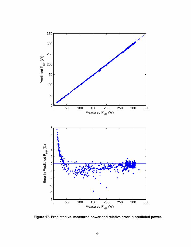
Figure 11. Determination of RSH0 (top) and RS0 (bottom). ...................................................... 36 Figure 12. I-V Curves at STC for simulated modules. ............................................................ 37 Figure 13. Irradiance and temperature conditions for model validation. ................................. 41 Figure 14. Error (percent) in performance parameters for fitted I-V curves. .......................... 41 Figure 15. Predicted vs. measured voltage and current. .......................................................... 42 Figure 16. Relative error (percent) in predicted voltage and current. ...................................... 43 Figure 17. Predicted vs. measured power and relative error in predicted power. .................... 44

TABLES Table 1. Parameters for simulated modules for method verification. ...................................... 38 Table 2. Estimation errors (percent) for model and performance parameters. ........................ 39 Table 3. Estimation errors (percent) for model and performance parameters when using exact

diode factor. ......................................................................................................................... 40 Table 4. Estimated model parameters for validation data. ....................................................... 42

7

NOMENCLATURE DOE Department of Energy SAPM Sandia Array Performance Model SNL Sandia National Laboratories STC standard test conditions

8

9

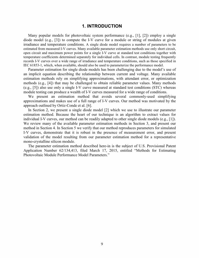
1. INTRODUCTION Many popular models for photovoltaic system performance (e.g., [1], [2]) employ a single

diode model (e.g., [3]) to compute the I-V curve for a module or string of modules at given irradiance and temperature conditions. A single diode model requires a number of parameters to be estimated from measured I-V curves. Many available parameter estimation methods use only short circuit, open circuit and maximum power points for a single I-V curve at standard test conditions together with temperature coefficients determined separately for individual cells. In contrast, module testing frequently records I-V curves over a wide range of irradiance and temperature conditions, such as those specified in IEC 61853-1, which, when available, should also be used to parameterize the performance model.

Parameter estimation for single diode models has been challenging due to the model’s use of an implicit equation describing the relationship between current and voltage. Many available estimation methods rely on simplifying approximations, with attendant error, or optimization methods (e.g., [4]) that may be challenged to obtain reliable parameter values. Many methods (e.g., [5]) also use only a single I-V curve measured at standard test conditions (STC) whereas module testing can produce a wealth of I-V curves measured for a wide range of conditions.

We present an estimation method that avoids several commonly-used simplifying approximations and makes use of a full range of I-V curves. Our method was motivated by the approach outlined by Ortiz-Conde et al. [6].

In Section 2, we present a single diode model [2] which we use to illustrate our parameter estimation method. Because the heart of our technique is an algorithm to extract values for individual I-V curves, our method can be readily adapted to other single diode models (e.g., [1]). We review many of the available parameter estimation methods in Section 3, and present our method in Section 4. In Section 5 we verify that our method reproduces parameters for simulated I-V curves, demonstrate that it is robust in the presence of measurement error, and present validation of the model resulting from our parameter estimation method for a representative mono-crystalline silicon module.

The parameter estimation method described here-in is the subject of U.S. Provisional Patent Application Number 62/134,413, filed March 17, 2015, entitled “Methods for Estimating Photovoltaic Module Performance Model Parameters.”

10

11

2. SINGLE DIODE MODELS A model for the electrical characteristic of a solar cell (e.g., [2], Eq. 1) can be derived from

physical principles (e.g., [3]) and is often formulated as an equivalent circuit comprising a current source, a diode, a parallel resistor and a series resistor (Figure 1). For a module comprising SN identical cells in series, use of the Shockley diode equation and summation of the indicated currents results in the single diode equation for the module’s I-V characteristic ([3], Eq. 3.154):

exp 1S SL O

th SH

V IR V IRI I InV R

+ += − − −

(1)

where LI is the photo-generated current (A),

OI is the dark saturation current (A), n is the diode ideality factor (unitless),

th S CV N kT q= is termed the thermal voltage (V) for the module, which is determined from cell temperature CT (K), Boltzmann’s constant k (J/K) and the elementary charge q (coulomb),

k is Boltzmann’s constant ( 231.38066 10 J/K−× ), q is the elementary charge ( 191.60218 10 coulomb−× ),

SR is the series resistance (Ω),

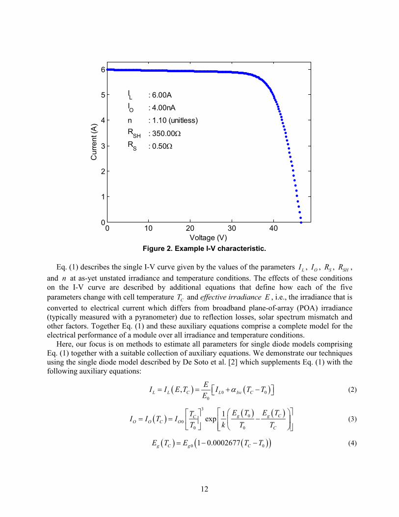
SHR is the shunt resistance (Ω). In this report, values for SR and SHR are considered at the module level; average values for the cells comprising a module can be obtained from the module values (e.g., [7]). Figure 2 displays an example I-V characteristic.

Figure 1. Single diode equivalent circuit for a PV cell or module.

12

0 10 20 30 400

1

2

3

4

5

6

IL : 6.00AIO : 4.00nA

n : 1.10 (unitless)R

SH : 350.00ΩR

S : 0.50Ω

Voltage (V)

Cur

rent

(A)

Figure 2. Example I-V characteristic.

Eq. (1) describes the single I-V curve given by the values of the parameters LI , OI , SR , SHR ,

and n at as-yet unstated irradiance and temperature conditions. The effects of these conditions on the I-V curve are described by additional equations that define how each of the five parameters change with cell temperature CT and effective irradiance E , i.e., the irradiance that is converted to electrical current which differs from broadband plane-of-array (POA) irradiance (typically measured with a pyranometer) due to reflection losses, solar spectrum mismatch and other factors. Together Eq. (1) and these auxiliary equations comprise a complete model for the electrical performance of a module over all irradiance and temperature conditions.

Here, our focus is on methods to estimate all parameters for single diode models comprising Eq. (1) together with a suitable collection of auxiliary equations. We demonstrate our techniques using the single diode model described by De Soto et al. [2] which supplements Eq. (1) with the following auxiliary equations:

( ) ( )0 00

,L L C L Isc CEI I E T I T TE

α= = + − (2)

( ) ( ) ( )30

00 0

1exp g g CCO O C O

C

E T E TTI I T IT k T T

= = −

(3)

( ) ( )( )0 01 0.0002677g C g CE T E T T= − − (4)

13

( ) 00SH SH SH

ER R E RE

= = (5)

0S SR R= (6)

0n n= (7)

In Eq. (2) through Eq.(7), the subscript 0~ indicates a value at the reference conditions 0E and

0T for irradiance and cell temperature, respectively; typical values are 0E =1000 W/m2 and

0T =298K. Other choices are available for the auxiliary equations, the use of which results in different single diode models (e.g., [1]).

In this paper we refer to Eq. (1) as the single diode equation and to Eq. (1) together with auxiliary equations as the single diode model. The term “five parameter model” is often used to refer to a single diode model that incorporates Eq. (1); this term arises from the presence of the coefficients LI , OI , SR , SHR , and n which are commonly referred as the “five parameters.” The term “five parameter model” is imprecise when used to refer to a complete model comprising Eq. (1) along with the auxiliary equations, because the auxiliary equations contain the model’s parameters whereas the single diode equation itself does not. For the exemplary single diode model considered here, the parameters are 0n , 0OI , 0LI , 0SHR , 0SR and 0gE , and Iscα ; it is these values which must be determined from measurements, i.e., from a set of I-V curves measured at various levels of irradiance and cell temperature.

14

15

3. REVIEW OF AVAILABLE PARAMETER ESTIMATION METHODS A successful parameter estimation method should satisfy the following criteria: 1) robust – the method should obtain parameter values for a wide range of module

technologies and in the presence of reasonable measurement errors. 2) reliable – the method should obtain the same parameter values repeatedly when applied

to the same data by different analysts. 3) accessible – the method should be fully documented and readily implemented and used

by anyone with an adequate general background in PV modeling and in numerical analysis techniques.

We use these criteria to guide our review of existing methods, although we do not attempt to assign quantitative ratings to different methods according to these criteria.

The literature describing proposed methods for extracting values for the five parameters appearing in Eq. (1) is extensive; as early as 1986, proposed methods were sufficiently numerous to merit comparative studies (e.g., [8]). A recent survey of published methods is found in [6]. Here, we do not attempt a comprehensive literature survey; instead we cite examples that illustrate different approaches to parameter estimation and comment on the obstacles to meeting the criteria of reliability, precision and robustness. We emphasize that all published methods we reviewed were successful in extracting parameters for which the computed I-V curves reasonably matched the data. We considered these numerically successful methods in light of our criteria — robustness; reliability; and accessiblity — to identify methods which could be candidates for a widely-adopted standard.

Some proposed methods (e.g., [9]; [10]) simplify or replace the diode equation Eq. (1)) to overcome its implicit nature before extracting parameters. We did not pursue these techniques, because fundamentally, they estimate parameter values for a model different than that described by Eq. (1).

Techniques that do not simplify the diode equation can be divided roughly into two categories: methods that use only a manufacturer’s data sheet, (e.g., [11]); and methods that use, in some manner, a range of I-V curves. Here, we do not investigate approaches that use only data sheet information although that problem is of significant practical interest; our focus is on obtaining model parameters from a set of measured I-V curves.

Most methods find values for parameters by solving a system of non-linear equations. Typically, a system of non-linear equations is formulated by evaluating Eq. (1) at specific conditions to obtain equations corresponding to different points on the I-V curve and minimizing the difference between these points and the corresponding measured values. For example, [2], [7] and [5] evaluate Eq. 1 at standard test conditions (STC) for the short-circuit, open-circuit and maximum power points and subtract the measured values to obtain three equations involving five unknowns; a fourth equation is obtained by setting 0dP dV = at the maximum power point, and a fifth equation is obtained by translating an I-V curve to a cell temperature different from STC (using temperature coefficients determined by some other method). Other proposed methods obtain a system of equations by making approximations to Eq. (1) over parts of its domain (e.g., [12], [13]) or to equations derived from Eq. (1) (e.g., [14], [15], [16]). The system of equations is then solved by a numerical technique: proposed methods include root-finding (e.g., [4], [7]) and global optimization (e.g., [17], [18]). We note that these methods require nested numeric evaluations: (i) to solve Eq. (1) for current (or voltage) (e.g., [4]) for particular values for parameters, and (ii) to adjust parameter values to minimize the error metric.

16

Root-finding and optimization methods require initial estimates of parameter values, selection of an error metric, and setting of conditions to determine convergence. Different choices for these aspects may result in different parameter values being obtained from the same data set. From the point of view of our desired criteria, the primary weakness of parameter estimation methods using root-finding and optimization techniques is achieving reliability because it is common for these methods to fail to converge unless initial estimates of parameters are sufficiently close to optimum. Reliability may be achieved by proscribing initial conditions, error metrics and convergence tolerances, if practical, although evidence suggests that proscribed initial conditions may in turn compromise robustness (e.g., [4]).

A challenge common to all parameter estimation methods arises from the widely disparate magnitudes of terms appearing in Eq. (1). For V near OCV , for a 72-cell module the argument

( )S S thV IR N nV+ of the exponential term in Eq. (1) takes values on the order of 30 (i.e.,

( )30 50 72 1.1 0.02sIR≈ + × × ). Unless SHR is unreasonably small (i.e., on the order of 5Ω ) so

that the term ( )S SHV IR R+ becomes comparable to the photocurrent 8ALI ≈ , LI must be

offset by ( )exp 1O S S thI V IR N nV + − in order for current I to be near 0. Consequently in

this region of the I-V curve ( ) 13exp 30 10OI −≈ − ≈ , and relatively small changes in the estimated value for the diode factor n (e.g., from 1.1 to 1.15) cause large changes to the value for OI (e.g., by a factor of more than 3). Multivariable optimization techniques, particularly root-finding methods that rely on derivatives (e.g., Newton’s method) or on domain partitioning (e.g., the Nelder-Mead method) may be challenged to overcome these greatly different scales and update individual parameter values appropriately.

Many methods simplify the system of equations by estimating certain parameters directly from the data by means of approximations. Commonly, e.g., [15], [19], SHR is approximated as

SC

SHI I

dVRdI =

≈ − (8)

from which a value for SHR is obtained by some kind of numerical differentiation or curve fitting. The value for SHR is then imposed when estimating the remaining parameters. While these methods appeal due to the reduction in dimension of the optimization problem, the resulting parameter values are likely to be biased, or result in inconsistencies among the parameter values for an I-V curve (i.e., Eq. (1) becomes an inequality) due to biases inherent in the approximation. For example, if Eq. (8) is used, the values for SR are likely to be unreasonably small; see Appendix E for details.

Other methods (e.g., [12], [14], [20]) simplify the resulting system of equation by dividing [ ]0, OCV into several intervals and formulating different systems of equations for each interval. Within a given interval the system of equations may be simplified by approximations and certain parameters are estimated from data in regions where those parameters are most influential. These methods are often attractive because they can be motivated by the behavior of the physical system being modeled. However, they are also difficult to formulate to meet the reliability criterion. The boundaries between the intervals comprising [ ]0, OCV must be defined, which often is done by visual examination of data rather than algorithmically, and different choices of

17

boundaries will result in different subsets of data being used to estimate each parameter with consequent differences in parameter values.

Among the surveyed literature we found several approaches ([6], [21], [22]) that consider the full range of each I-V curve and make no simplifying approximations. For example, [6] and [21] fit the integrated single diode equation to corresponding integrated data by regression instead of estimating coefficients by fitting the single diode equation (Eq. (1)) to data directly; these methods differ in the variable of integration (voltage in the case of [6]; current in the case of [21]). Fitting to integrated data may offer the advantage of suppressing the effects of random measurement error. Our proposed method (Section 4.2) was initially motivated by [6]. However, upon implementation and testing of [6], we found problems stemming from the use of regression. Colinearity of the predictors in the regression and inaccuracy in the numerical integration procedure compromised the method’s reliability resulting in parameter values which were unduly sensitive to small changes in the data. We attempted to overcome these problems by adding elements of our own innovation.

Finally, [22] fits the derivative dI dV determined from the single diode equation to values estimated by numerical differentiation of measured I-V curves. Error in the measurements of current and/or voltage may be amplified by direct numerical differentiation; consequently, the method in [22] smooths the data by fitting polynomials before differentiation, a step which may not be necessary for methods using integrated quantities.

18

19

4. NEW PARAMETER ESTIMATION METHOD Here we present an algorithm for estimating the parameters for the single diode model

outlined in Section 2. The core of the algorithm is a technique for fitting the single diode equation (Eq. (1)) to each of a set of measured I-V characteristics, thus obtaining, for each I-V curve, a set of five coefficient values (i.e., LI , OI , SR , SHR , and n ). Parameter values for the single diode model are then obtained by regressing the coefficients onto the irradiance and temperature conditions at which each I-V curve was measured.

The algorithm is demonstrated for the single diode model described in [2] but, with suitable modification, can be applied to any single diode model incorporating Eq. (1).

We first describe techniques for solving Eq. (1) analytically and numerically (Sect. 4.1) followed by an outline of our parameter estimation algorithm (Sect. 4.2).

4.1. Analytic and Numerical Solutions for Single Diode Equation Eq. (1) cannot be solved for current (or voltage) explicitly using elementary functions.

However, current can be expressed as a function of voltage ( )I I V= (or ( )V V I= ) by using the transcendental Lambert’s W function [23] as presented by several authors ([24], [25]). Lambert’s W function is the solution ( )W x of the equation ( ) ( )expx W x W x= . Using this function we

may write ( )I I V= :

( ) ( )exp S L OSH th S O SH SHL O

SH S SH S S th SH S SH S th

R I I VR nV R I R RVI I I WR R R R R nV R R R R nV

+ + = + − − + + + +

(9)

or ( )V V I= ; see Appendix A for the derivations.

( ) ( )exp L O SHO SHL O SH S th

th th

I I I RI RV I I I R IR nV WnV nV

+ − = + − − −

(10)

For convenience we introduce two variables

( )exp S L OS O SH SH

th SH S SH S th

R I I VR I R RnV R R R R nV

θ+ +

= + + (11)

and

( )exp L O SHO SH

th th

I I I RI RnV nV

ψ+ −

=

(12)

which permit Eq. (9) and Eq. (10) to be written compactly as

( ) ( )SH thL O

SH S SH S S

R nVVI I I WR R R R R

θ= + − −+ +

(13)

and

20

( ) ( )L O SH S thV I I I R IR nV W ψ= + − − − (14)

respectively. Lambert’s W function can be efficiently evaluated with very high precision [26]; thus Eq. (9)

and Eq. (10) can be directly implemented for most of the range of an I-V curve. However, for Eq. (10) approaching OCV (i.e., as current I becomes small), numerical overflow becomes a problem. For example, for 910 AOI −= , 1000SHR = Ω , 1.05n = , 6 ALI = (typical for a 72 cell module), and 1.973thV = , the argument ψ of the W function in Eq. (10) exceeds numerical overflow for 64-bit machines (approximately 30810 ) for 4.5 AI < . To compute this portion of the I-V curve we use logarithms as described in Appendix B.

4.2. Method Description We propose a sequential approach to obtaining single diode model parameters from measured

I-V curves. Throughout the process, we solve Eq. (1) using Lambert’s W function (e.g., by Eq. (9) and Eq. (10)). Using Lambert’s W function confers several advantages:

− Numerical computation is quite fast, requiring very little iteration. By contrast, other parameter estimation methods (e.g., [4]) solve Eq. (1) using fixed-point methods, which may require significantly more computational effort;

− Derivatives (e.g., dI dV ) can also be expressed exactly using the W function avoiding the pitfalls of estimating derivatives numerically;

− Asymptotic approximations for W are relatively simple which allows certain parameter estimation steps to be confirmed analytically.

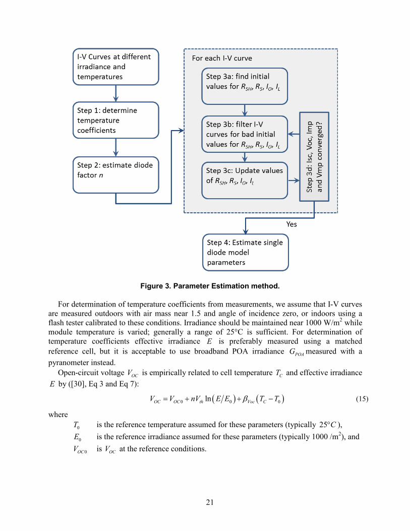
Figure 3 illustrates our parameter estimation method. We illustrate the steps of our method using data measured on a two-axis tracker for a 96-cell (i.e., 96SN = ), mono-crystalline cSi module.

Step 1: Temperature coefficients. We first determine temperature coefficients Iscα and Vocβ for short-circuit current SCI and

open-circuit voltage OCV , respectively, from I-V curves with irradiance near STC (i.e., 1000 W/m2). We employ linear regression as specified in IEC 60891 [27] and as has been extensively and successfully used ([28], [29]) for the Sandia Array Performance Model (SAPM) [30]. Only

Iscα appears explicitly in the performance model outlined in Sect. II, although to apply Step 2 of our method to the exemplary single diode model [2] we also need Vocβ .

21

Figure 3. Parameter Estimation method. For determination of temperature coefficients from measurements, we assume that I-V curves

are measured outdoors with air mass near 1.5 and angle of incidence zero, or indoors using a flash tester calibrated to these conditions. Irradiance should be maintained near 1000 W/m2 while module temperature is varied; generally a range of 25°C is sufficient. For determination of temperature coefficients effective irradiance E is preferably measured using a matched reference cell, but it is acceptable to use broadband POA irradiance POAG measured with a pyranometer instead.

Open-circuit voltage OCV is empirically related to cell temperature CT and effective irradiance E by ([30], Eq 3 and Eq 7):

( ) ( )0 0 0lnOC OC th Voc CV V nV E E T Tβ= + + − (15)

where 0T is the reference temperature assumed for these parameters (typically 25 C° ),

0E is the reference irradiance assumed for these parameters (typically 1000 /m2), and

0OCV is OCV at the reference conditions.

22

Appendix D demonstrates that the empirical relationship between OCV and E in Eq. (15) is asymptotically consistent with the single diode model described in Sect. 2. The linear relationship between OCV and CT is outlined for the single diode model in [3], Eq. 3.165.

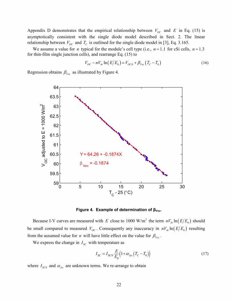
We assume a value for n typical for the module’s cell type (i.e., 1.1n = for cSi cells, 1.3n = for thin-film single junction cells), and rearrange Eq. (15) to

( ) ( )0 0 0lnOC th OC Voc CV nV E E V T Tβ− = + − (16)

Regression obtains Vocβ as illustrated by Figure 4.

0 5 10 15 20 25 3059

59.5

60

60.5

61

61.5

62

62.5

63

63.5

64

Y = 64.26 + -0.1874X

βVoc

= -0.1874

TC

- 25 (°C)

VO

C a

djus

ted

to E

= 1

000

W/m

2

Figure 4. Example of determination of βVoc. Because I-V curves are measured with E close to 21000 W/m the term ( )0lnthnV E E should

be small compared to measured OCV . Consequently any inaccuracy in ( )0lnthnV E E resulting from the assumed value for n will have little effect on the value for Vocβ .

We express the change in SCI with temperature as

( )( )0 00

1 IscSC SC CEI I T TE α= + − (17)

where 0SCI and Iscα are unknown terms. We re-arrange to obtain

23

( )( )

( )

00

0 1 0

1SC SC Isc C

C

EI I T TE

T T

α

β β

= + −

= + − (18)

Using measured SCI , E and CT , a linear, least-squares regression obtains coefficients 0β and

1β , from which Iscα is determined:

1 0Iscα β β= . (19)

Figure 5 illustrates the determination of Iscα .

0 5 10 15 20 25 305.88

5.89

5.9

5.91

5.92

5.93

5.94

5.95

5.96

5.97

Y = 5.89 + 0.00187X

aIsc

= 0.00187/5.8929 = 0.000317

TC

- 25 (°C)

I SC

adj

uste

d to

E =

100

0 W

/m2

Figure 5. Example of determination of αIsc. Step 2: Diode factor. In the exemplary single diode model [2], n is considered to have the same, constant value for

all conditions. We estimate n from the relationship between OCV and effective irradiance E . From Eq. (10) we obtain

( ) ( )exp L O SHO SHOC L O SH th

th th

I I RI RV I I R nV WnV nV

+ = + −

(20)

24

Asymptotic analysis (Appendix D) shows that when 0CT T= , to first order

( )0 0lnOC OC thV V nV E E− ≈ (21)

which is the same expression as is used in [30] (i.e., Eq. (15) in this presentation). Accordingly, we use Eq. (15) to obtain n from a linear regression:

( ) ( )0 0 0lnOC Voc C OC thV T T V nV E Eβ− − = + (22)

Figure 6 illustrates the determination of n . For the regression in Figure 6, I-V curves are required over a range of irradiance, preferably from 400 W/m2 to 1000 W/m2.

-8 -6 -4 -2 0 251

52

53

54

55

56

57

58

59

60

61

VOC

- βVoc

× (TC

- 50)

Vth

× ln

(E /

1000

)

Y = 60.04 + 1.17Xn = 1.17

DataModel

Figure 6. Example of determination of n.

Step 3. Values for RSH, RS, IO and IL for each I-V curve. These parameters are estimated using an iterative procedure: initial estimates are obtained,

and then the estimates are updated sequentially until convergence criteria are satisfied.

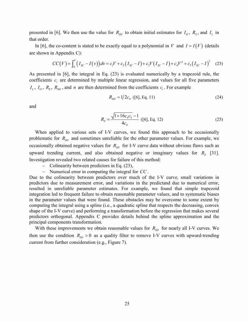
Step 3a: Initial estimates. For each I-V curve, we determine an initial value for SHR , SR , OI and LI . We obtain the initial estimate for SHR with a regression involving the co-content CC , i.e., an integral of the I-V curve over voltage, which method is an improvement upon that

25

presented in [6]. We then use the value for SHR to obtain initial estimates for OI , SR , and LI in that order.

In [6], the co-content is stated to be exactly equal to a polynomial in V and ( )I I V= (details are shown in Appendix C):

( ) ( )( ) ( ) ( ) ( )221 2 3 4 50

V

SC SC SC SCCC V I I v dv c V c I I c V I I c V c I I= − = + − + − + + −∫ (23)

As presented in [6], the integral in Eq. (23) is evaluated numerically by a trapezoid rule, the coefficients ic are determined by multiple linear regression, and values for all five parameters

LI , OI , SR , SHR , and n are then determined from the coefficients ic . For example

41 2SHR c= ([6], Eq. 11) (24)

and

4 5

4

1 16 14S

c cR

c+ −

= ([6], Eq. 12) (25)

When applied to various sets of I-V curves, we found this approach to be occasionally problematic for SHR and sometimes unreliable for the other parameter values. For example, we occasionally obtained negative values for SHR for I-V curve data without obvious flaws such as upward trending current, and also obtained negative or imaginary values for SR [31]. Investigation revealed two related causes for failure of this method:

− Colinearity between predictors in Eq. (23), − Numerical error in computing the integral for CC .

Due to the colinearity between predictors over much of the I-V curve, small variations in predictors due to measurement error, and variations in the predictand due to numerical error, resulted in unreliable parameter estimates. For example, we found that simple trapezoid integration led to frequent failure to obtain reasonable parameter values, and to systematic biases in the parameter values that were found. These obstacles may be overcome to some extent by computing the integral using a spline (i.e., a quadratic spline that respects the decreasing, convex shape of the I-V curve) and performing a transformation before the regression that makes several predictors orthogonal. Appendix C provides details behind the spline approximation and the principal components transformation.

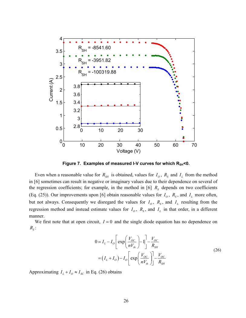
With these improvements we obtain reasonable values for SHR for nearly all I-V curves. We then use the condition 0SHR > as a quality filter to remove I-V curves with upward-trending current from further consideration (e.g., Figure 7).

26

0 10 20 30 40 50 60 700

0.5

1

1.5

2

2.5

3

3.5

4

RSH

= -8541.60

RSH

= -3951.82

RSH

= -100319.88

Voltage (V)

Cur

rent

(A)

0 10 20 302.8

3

3.2

3.43.6

3.8

Figure 7. Examples of measured I-V curves for which RSH<0. Even when a reasonable value for SHR is obtained, values for OI , SR and LI from the method

in [6] sometimes can result in negative or imaginary values due to their dependence on several of the regression coefficients; for example, in the method in [6] SR depends on two coefficients (Eq. (25)). Our improvements upon [6] obtain reasonable values for OI , SR , and LI more often, but not always. Consequently we disregard the values for OI , SR , and LI resulting from the regression method and instead estimate values for OI , SR , and LI in that order, in a different manner.

We first note that at open circuit, 0I = and the single diode equation has no dependence on SR :

( )

0 exp 1

exp

OC OCL O

th SH

OC OCL O O

th SH

V VI InV R

V VI I InV R

= − − −

= + − −

(26)

Approximating L O SCI I I+ ≈ in Eq. (26) obtains

27

0 exp OC OCSC O

th SH

V VI InV R

≈ − −

(27)

The initial estimate of OI is obtained from Eq. (27):

expOC OCO SC

SH th

V VI IR nV

= − −

(28)

With a value for OI in hand, the initial estimate of SR is obtained from the slope of the I-V

curve near OCV (but not at OCV ). Ideally, the derivative dIdV

will be negative and smoothly

decreasing as OCV V→ . Estimating the derivative from data requires use of some kind of numeric differentiation scheme. For measured I-V curves we cannot assume that the points comprising the I-V curve are taken at equally-spaced voltage values and consequently most common finite difference approximations (e.g., [32]) are not suitable. We employ a fifth order finite difference technique (i.e., Eq. A5b in [33]) which accommodates unequally-spaced data to estimate

( ) , 1, ,V kk

dII V k MV VdV

′ = ==

(29)

for data at voltages kV where 0.5 0.9OC k OCL V V V R= < < = and 1, ,k M= . Then, we estimate

SR as the average (Eq. (30))

,1

1 M

S S kk

R RM =

≅ ∑ (30)

where

( )( ), ln 1th th kS k SH V k

SC SH O th

nV nV VR R I VI R I nV

′= − + −

(31)

for points where ( ) 1 0SH V kR I V′ + < .

Eq. (30) is derived from the exact expression for dIdV

as follows: Writing for simplification

( ) ( )exp S L OS O SH SH

th SH S SH S th

R I I VR I R RVnV R R R R nV

θ θ+ +

= = + + (32)

and then differentiating Eq. (9) we obtain:

( )( )

( )

1 11

1 11 11

SH

SH S S

SH

SH S S

WRdIdV R R R W

RR R R W

θθ

θ

= − + + +

= − + − + +

(33)

28

For most of the range of voltage of interest, we may assume that 1θ << , consequently

( )W θ θ≈ [23], and hence ( )

1 1 11 1W

θθ θ

≈ ≈ −+ +

. Thus we obtain

1 1 SH

SH S S

RdIdV R R R

θ

≈ − + + (34)

Typically S SHR R<< and we also assume L O SCI I I+ ≈ so

expS O S SC

th th

R I R I VnV nV

θ +

≈

(35)

Combining Eq. (34) and Eq. (35)

1 1

1 exp

SH

SH S

SH O S SCSH

th th

RdIdV R R

R I R I VdIRdV nV nV

θ

≈ − +

+− ≈ +

(36)

which we solve for SR to obtain Eq. (31). When estimating an initial value for SR , care must be taken to exclude voltage points kV

where the term ( ) 1 0SH V kR I V′ + > , which can occur for either a positive value for ( )V kI V′ ,

indicative of questionable I-V curve data, or a negative but very small value for ( )V kI V′ , which may occur for V substantially less than MPV . However, we found it necessary to include voltages less than MPV in the average in Eq. (30) to obtain reasonable values for . We chose 0.5 OCL V= and 0.9 OCR V= , where the right limit is set to exclude points where the numerical derivative

( )V kI V′ becomes inaccurate due to a lack of measurements or due to the assumption that 1θ << which may fail for V very near OCV .

Lastly, LI is estimated by evaluating Eq. (1) at SCI :

exp S SC S SCL SC O O

th SH

R I R II I I InV R

= − + +

(37)

Step 3b: Filter out I-V curves with bad parameter sets. Once initial estimates are obtained, the

algorithm filters the parameter sets to exclude I-V curves where the parameter estimates indicate problems. An I-V curve is excluded if the corresponding parameter estimates meet any of the following criteria:

− The value for SHR is negative (indicating that current may be increasing with increasing voltage) or is indeterminate (indicating a lack of data or a problem with the regression which determines the coefficient 4c in Eq. (24)).

29

− The value for SR is negative, has a non-zero imaginary component, is indeterminate or is greater than SHR .

− The value for OI is zero, negative, or has a non-zero imaginary component. In addition, the algorithm expects that the PV device is substantially linear, i.e., the measured short-circuit current SCI is nearly proportional to effective irradiance E (or to broadband POA irradiance POAG ). An empirical efficiency η is obtained by regressing SCI onto E , i.e.:

0

SCEIE

η= (38)

and the residual ( )0 SCE E Iε η= − is used to exclude I-V curves where 0.05 SCIε > reasoning that these errors occur when there are substantial differences between E (or POAG ) and SCI due to shading or other external factors. When these rules are applied to data obtained at SNL’s laboratory typically only a few (<1%) I-V curves are filtered out, and these I-V curves usually display obvious problems such as increasing current as voltage increases.

Step 3c: Update initial estimates of SHR , SR , OI and LI to obtain final values for each I-V curve. The initial estimates SHR , SR , OI and LI may result in poor matches to measured OCV ,

MPV and MPI . Parameters are updated in order as follows:

1. SHR is adjusted to match MPV by a fixed point iteration, using previous values for SR ,

OI and LI ; 2. SR is updated to match MPV calculated using the new value for SHR and previous

values for OI and LI ; 3. OI is adjusted to match OCV by a method similar to Newton’s method using new

values for SHR and SR and the previous value for LI ; 4. LI is updated to match SCI by Eq. (37) using new values for SHR , SR and OI .

To adjust SHR we use Eq. (10) evaluated at the maximum power point:

( ) ( ) ( )MP L O SH MP SH S thV I I R I R R nV W ψ= + − + − (39)

where

( )exp SH L O MPO SH

th th

R I I II RnV nV

ψ+ −

=

(40)

However, Eq. (40) holds for any point ( ),V I on the I-V curve. Consequently we use a second equation which defines the maximum power point:

( ) ( ) ( )( ) ( )0

1L O MP SH MP S th MP SH SH SMP

WdP I I I R I R nV W I R R RI IdI W

ψψ

ψ

= = + − − − + − + = + (41)

30

Solving Eq. (39) and Eq. (41) for SR and equating the results to eliminate SR we obtain an expression involving SHR , OI , LI and the measured maximum power point ( ),MP MPV I :

( ) ( ) ( )( )

0 ,2 2 1 2

thL O SHMPSH O L SH

MP MP MP

nV W WI I RVf R I I RI I I W

ψ ψψ

+= = − − −

+ (42)

We solve for the updated value of SHR by fixing OI and LI at their previous values and applying fixed point iteration to the following re-arrangement of Eq. (42):

( )

( )( )

, 1 ,

1 2thL O MPSH k SH k

MP MP MP

W nV WI I VR RW I I I

ψ ψψ+

+ += − −

(43)

Numerical tests with measured I-V curves for modules with a variety of cell technologies (including cSi and thin-film cells) indicate that Eq. (43) converges, although the rate of convergence is slow. Analytic proof that Eq. (43) is a contraction mapping appears formidable to accomplish; we see this part of the algorithm as an opportunity for research and improvement.

With an adjusted value for SHR the value for SR is updated to be consistent with the new value for SHR and the measured maximum power point using Eq. (39):

( )L O MP th MPS SH

MP MP MP

I I I nV VR R WI I I

ψ+ −= − − (44)

Next, OI is adjusted so that calculated OCV matches measured OCV . Consider ( )OC OV I as a function of only OI (i.e., using Eq. (20) and fixing all parameters other than OI at their current

values) and denote the measured OCV by OCV . We seek a value OCI such that ( )ˆ ˆ 0OC OC OCV I V− =

and use a root-finding method akin to Newton’s method. Differentiating Eq. (20) with respect to OI we obtain:

( )( )

11

OCOC SHSH th

O OC O th

WdV RR nVdI W I nV

ψψ

= − + +

(45)

where

( )exp L O SHO SH

OCth th

I I RI RnV nV

ψ+

=

(46)

For most conceivable modules, we can safely assume that 1OCψ >> . The term

( )exp L O SH

th

I I RnV+

in Eq. (46) is orders of magnitude greater than the term O SH

th

I RnV

. For

example, taking 710OI A−− , a relatively large value, ~ 1LI A which is small for most modules,

2thnV − ,and ~ 100SHR Ω , a relatively small value, leads to

31

( )7

7 1410 100 100exp 10 exp 50 102 2OCψ

−−×

− − − (47)

Because we may assume that 1OCψ >> , we may also assume that ( )( )

11

OC

OC

WWψψ

≈+

simplifying

Eq. (45) to

OC th

O O

dV nVdI I

−≈ (48)

Approximating OCV as a linear function of OI near OCI :

( ) ( )*ˆ ˆOC

OC O OC O OO OO

dVV I V I II IdI

≈ + × −=

(49)

where the derivative is evaluated at *OI also near OCI . Because the curve described by

( )( ),O OC OI V I is concave upwards (per Eq. (48)) a better estimate of ( )OC OV I is obtained from

Eq. (49) by evaluating the derivative at the midpoint *ˆ

2O OI II +

= between OI and OI .

Combining Eq. (48) and Eq. (49)

( ) ( )

( )

ˆ ˆ

2ˆ ˆˆ

OCOC O OC O O

O

thOC O O

O O

dVV I V I IdI

nVV I II I

≈ + −

≈ − −+

(50)

Solving for OI obtains

( )( )( )( )( )( )

( )( )

ˆ 2ˆ

ˆ2

ˆ21

ˆ2

OC O OC thO O

th OC O OC

OC O OCO

th OC O OC

V I V nVI I

nV V I V

V I VI

nV V I V

− + ≈ − − − ≈ + − −

(51)

As in Newton’s method we iterate Eq. (51) to obtain a sequence of values ,O kI converging to OI :

( )( )

( )( ),

, 1 ,,

ˆ21

ˆ2OC O k OC

O k O kth OC O k OC

V I VI I

nV V I V+

− = × + − −

(52)

where we compute ( ),OC O kV I using Eq. (20). Convergence of Eq. (52) is rapid; in our testing ten iterations suffice.

32

Lastly, LI is updated to match measured SCI using updated values for SHR , SR and OI in Eq. (37).

Step 3d: Test for convergence. The parameter estimates for an I-V curve are considered

converged when the maximum difference between the predicted MPI , MPV and MPP and the corresponding measurements are all less than 0.002% of the measured values. We also fix an (arbitrary) upper limit on the number of iterations (e.g., 10). The threshold for precision and the iteration limit can be easily changed.

Step 4. Parameter values for single diode model equations. Step 3 results in a set of parameter values corresponding to each measured I-V curve. In step

4 we relate the parameter values for each I-V curve to the irradiance and temperature conditions extant when the I-V curve was measured to determine the appropriate parameters for each auxiliary equation. The regressions involved necessarily depend on the particular single diode model being considered. Here we show how the model parameters appearing in the auxiliary equations of the single diode model in [2] (i.e., Eq. (2) through Eq. (7)) are determined. The parameters to be estimated are: 0LI , 0OI , 0gE , 0SHR , 0SR and 0n . Throughout we recommend the use of a robust regression technique (e.g., iteratively reweighted least squares1) to minimize the effects of outlier data, e.g., unfiltered I-V curves where the module and the irradiance sensor were exposed to somewhat different irradiance conditions.

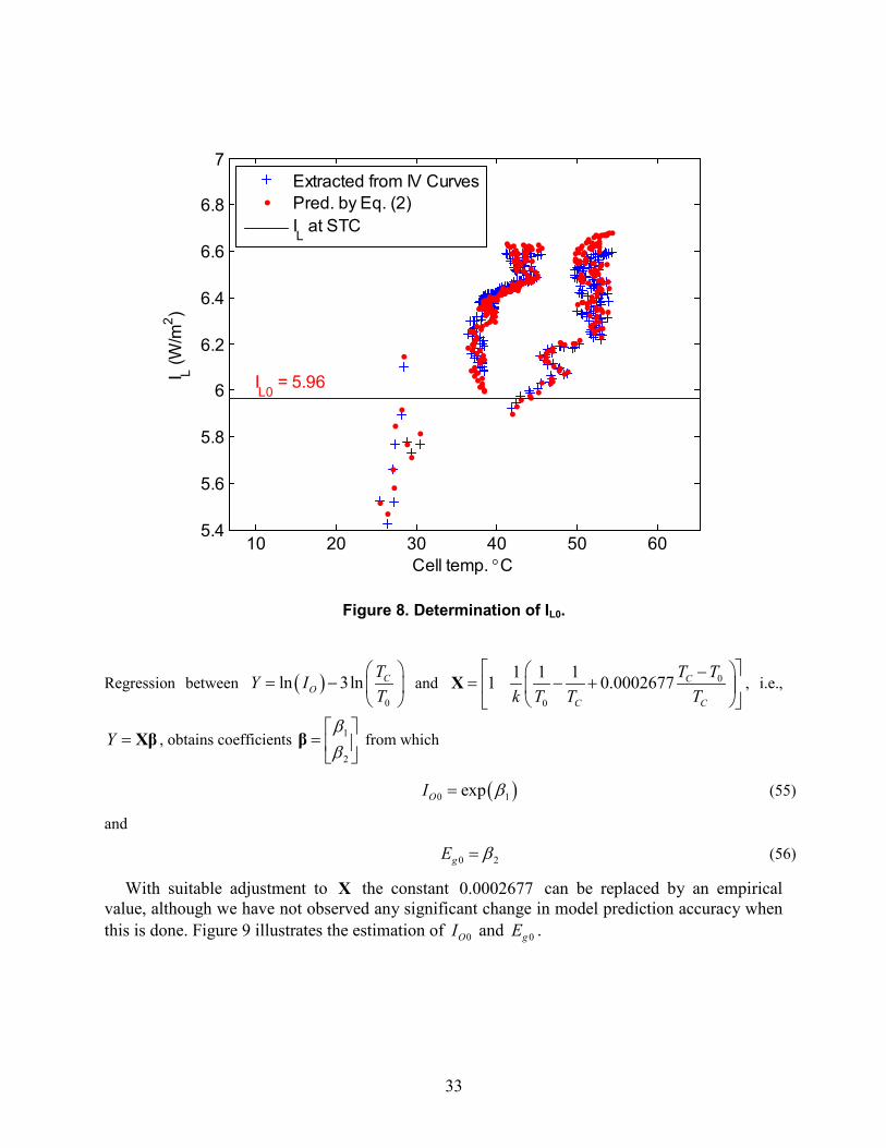
Light current at STC 0LI . 0LI is, by definition, the light current at STC conditions: POA irradiance of 1000 W/m2, cell temperature 25°C, and reference solar spectrum [34]. We estimate

0LI from a subset of values of LI determined for each of the N I-V curves by filtering for irradiance conditions near STC. In our example here, we select I-V curves with POA irradiance within 100 W/m2 of 1000 W/m2. Absolute (i.e., pressure adjusted) air mass AMa is often used as a surrogate for solar spectrum because it is easily calculated; we also filter for I-V curves within 0.5 units of 1.5AMa = . We estimate 0LI as the average of the values determined using Eq. (2) for each I-V curve in the selected subset indexed by 1, ,j M= :

( )00 , , 0

1

1 M

L L j Isc C jj j

EI I T TM E

α=

= − −

∑ (53)

A value for Iscα should be determined from separate testing as described in Section 4.2, Step 1. Figure 8 illustrates the estimate of 0LI .

Dark current 0OI and band gap 0gE . 0OI and 0gE are estimated jointly. Eq. (4) is substituted into Eq.

(3) and the result is re-arranged to obtain:

( ) ( ) 00 0

0 0

1 1 1ln 3ln ln 0.0002677C CO O g

C C

T T TI I ET k T T T

−− = + − +

(54)

1 E.g., http://www.mathworks.com/help/stats/robustfit.html

33

10 20 30 40 50 605.4

5.6

5.8

6

6.2

6.4

6.6

6.8

7

Cell temp. °C

I L (W/m

2 )

IL0

= 5.96

Extracted from IV CurvesPred. by Eq. (2)IL at STC

Figure 8. Determination of IL0.

Regression between ( )0

ln 3ln CO

TY IT

= −

and 0

0

1 1 11 0.0002677 C

C C

T Tk T T T

−= − +

X , i.e.,

Y = Xβ , obtains coefficients 1

2

ββ

=

β from which

( )0 1expOI β= (55)

and

0 2gE β= (56)

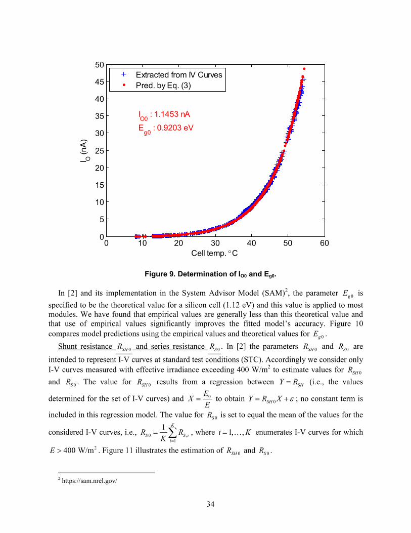
With suitable adjustment to X the constant 0.0002677 can be replaced by an empirical value, although we have not observed any significant change in model prediction accuracy when this is done. Figure 9 illustrates the estimation of 0OI and 0gE .

34

0 10 20 30 40 50 600

5

10

15

20

25

30

35

40

45

50

Cell temp. °C

I O (n

A)

IO0

: 1.1453 nA

Eg0

: 0.9203 eV

Extracted from IV CurvesPred. by Eq. (3)

Figure 9. Determination of IO0 and Eg0. In [2] and its implementation in the System Advisor Model (SAM)2, the parameter 0gE is

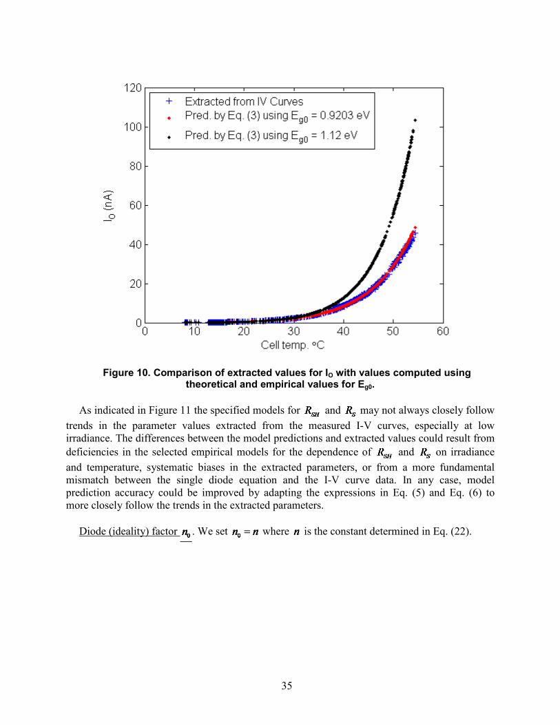
specified to be the theoretical value for a silicon cell (1.12 eV) and this value is applied to most modules. We have found that empirical values are generally less than this theoretical value and that use of empirical values significantly improves the fitted model’s accuracy. Figure 10 compares model predictions using the empirical values and theoretical values for 0gE .

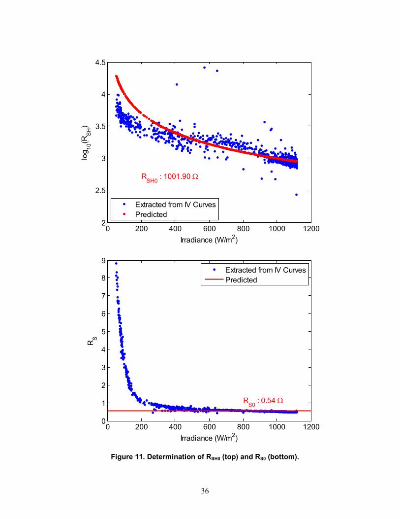
Shunt resistance 0SHR and series resistance 0SR . In [2] the parameters 0SHR and 0SR are intended to represent I-V curves at standard test conditions (STC). Accordingly we consider only I-V curves measured with effective irradiance exceeding 400 W/m2 to estimate values for 0SHR and 0SR . The value for 0SHR results from a regression between SHY R= (i.e., the values

determined for the set of I-V curves) and 0EXE

= to obtain 0SHY R X ε= + ; no constant term is

included in this regression model. The value for 0SR is set to equal the mean of the values for the

considered I-V curves, i.e., 0 ,1

1 K

S S ii

R RK =

= ∑ , where 1, ,i K= enumerates I-V curves for which

2400 W/mE > . Figure 11 illustrates the estimation of 0SHR and 0SR . 2 https://sam.nrel.gov/

35

Figure 10. Comparison of extracted values for IO with values computed using theoretical and empirical values for Eg0.

As indicated in Figure 11 the specified models for and may not always closely follow

trends in the parameter values extracted from the measured I-V curves, especially at low irradiance. The differences between the model predictions and extracted values could result from deficiencies in the selected empirical models for the dependence of and on irradiance and temperature, systematic biases in the extracted parameters, or from a more fundamental mismatch between the single diode equation and the I-V curve data. In any case, model prediction accuracy could be improved by adapting the expressions in Eq. (5) and Eq. (6) to more closely follow the trends in the extracted parameters.

Diode (ideality) factor . We set where is the constant determined in Eq. (22).

36

0 200 400 600 800 1000 12002

2.5

3

3.5

4

4.5

Irradiance (W/m2)

log 10

(RS

H)

RSH0

: 1001.90 Ω

Extracted from IV CurvesPredicted

0 200 400 600 800 1000 12000

1

2

3

4

5

6

7

8

9

Irradiance (W/m2)

RS

RS0

: 0.54 Ω

Extracted from IV CurvesPredicted

Figure 11. Determination of RSH0 (top) and RS0 (bottom).

37

5. VERIFICATION AND VALIDATION We verify the accuracy of our method by computing simulated I-V curves and then applying

our parameter estimation method to recover the parameters used to generate the simulated I-V curves. We validate our method by predicting outdoor performance of a representative module comprising mono-crystalline silicon cells. Parameters for a single diode model are estimated from a sample of I-V curves measured outdoors in Albuquerque, NM, and then module performance is predicted for measured, out-of-sample I-V curves.

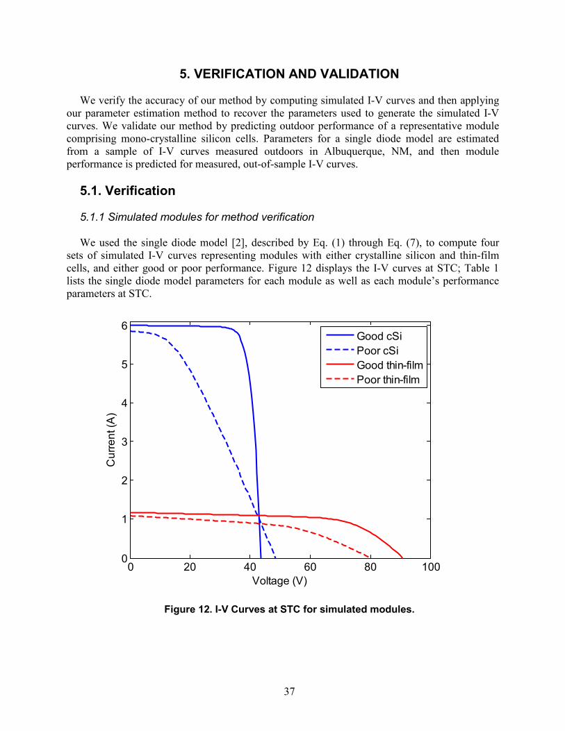
5.1. Verification 5.1.1 Simulated modules for method verification We used the single diode model [2], described by Eq. (1) through Eq. (7), to compute four

sets of simulated I-V curves representing modules with either crystalline silicon and thin-film cells, and either good or poor performance. Figure 12 displays the I-V curves at STC; Table 1 lists the single diode model parameters for each module as well as each module’s performance parameters at STC.

0 20 40 60 80 1000

1

2

3

4

5

6

Cur

rent

(A)

Voltage (V)

Good cSiPoor cSiGood thin-filmPoor thin-film

Figure 12. I-V Curves at STC for simulated modules.

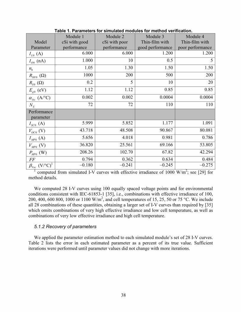
38

Table 1. Parameters for simulated modules for method verification.

Model Parameter

Module 1 cSi with good performance

Module 2 cSi with poor performance

Module 3 Thin-film with

good performance

Module 4 Thin-film with

poor performance 0LI (A) 6.000 6.000 1.200 1.200

0OI (nA) 1.000 10 0.5 5

0n 1.05 1.30 1.50 1.50

0SHR (Ω) 1000 200 500 200

0SR (Ω) 0.2 5 10 20

0gE (eV) 1.12 1.12 0.85 0.85

Iscα (A/°C) 0.002 0.002 0.0004 0.0004

SN 72 72 110 110 Performance

parameter

0SCI (A) 5.999 5.852 1.177 1.091

0OCV (V) 43.718 48.508 90.867 80.081

0MPI (A) 5.656 4.018 0.981 0.786

0MPV (V) 36.820 25.561 69.166 53.805

0MPP (W) 208.26 102.70 67.82 42.294 FF 0.794 0.362 0.634 0.484

Vocβ (V/°C)1 –0.180 –0.241 –0.245 –0.275 1 computed from simulated I-V curves with effective irradiance of 1000 W/m2; see [29] for

method details. We computed 28 I-V curves using 100 equally spaced voltage points and for environmental

conditions consistent with IEC-61853-1 [35], i.e., combinations with effective irradiance of 100, 200, 400, 600 800, 1000 or 1100 W/m2, and cell temperatures of 15, 25, 50 or 75 °C. We include all 28 combinations of these quantities, obtaining a larger set of I-V curves than required by [35] which omits combinations of very high effective irradiance and low cell temperature, as well as combinations of very low effective irradiance and high cell temperature.

5.1.2 Recovery of parameters We applied the parameter estimation method to each simulated module’s set of 28 I-V curves.

Table 2 lists the error in each estimated parameter as a percent of its true value. Sufficient iterations were performed until parameter values did not change with more iterations.

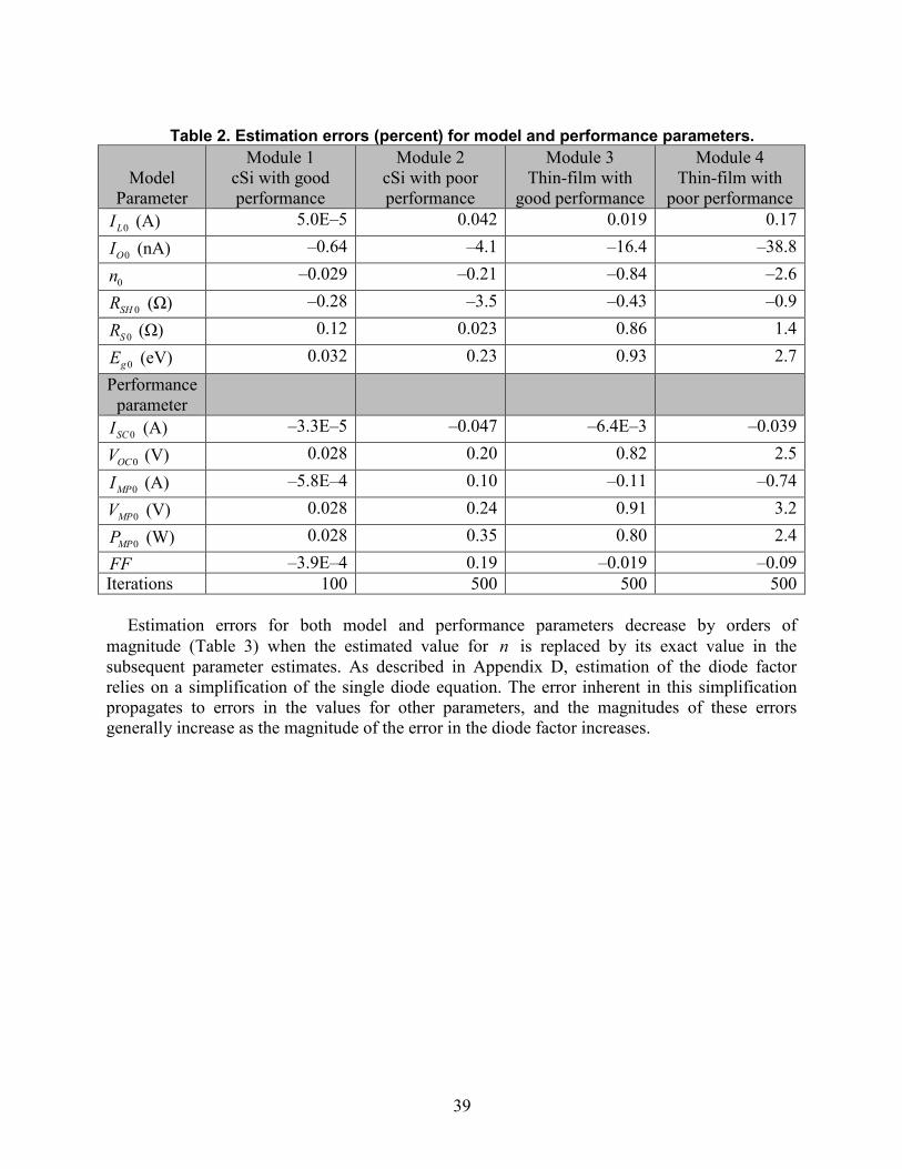
39

Table 2. Estimation errors (percent) for model and performance parameters.

Model Parameter

Module 1 cSi with good performance

Module 2 cSi with poor performance

Module 3 Thin-film with

good performance

Module 4 Thin-film with

poor performance 0LI (A) 5.0E–5 0.042 0.019 0.17

0OI (nA) –0.64 –4.1 –16.4 –38.8

0n –0.029 –0.21 –0.84 –2.6

0SHR (Ω) –0.28 –3.5 –0.43 –0.9

0SR (Ω) 0.12 0.023 0.86 1.4

0gE (eV) 0.032 0.23 0.93 2.7 Performance

parameter

0SCI (A) –3.3E–5 –0.047 –6.4E–3 –0.039

0OCV (V) 0.028 0.20 0.82 2.5

0MPI (A) –5.8E–4 0.10 –0.11 –0.74

0MPV (V) 0.028 0.24 0.91 3.2

0MPP (W) 0.028 0.35 0.80 2.4 FF –3.9E–4 0.19 –0.019 –0.09 Iterations 100 500 500 500

Estimation errors for both model and performance parameters decrease by orders of magnitude (Table 3) when the estimated value for n is replaced by its exact value in the subsequent parameter estimates. As described in Appendix D, estimation of the diode factor relies on a simplification of the single diode equation. The error inherent in this simplification propagates to errors in the values for other parameters, and the magnitudes of these errors generally increase as the magnitude of the error in the diode factor increases.

40

Table 3. Estimation errors (percent) for model and performance parameters when

using exact diode factor.

Model Parameter

Module 1 cSi with good performance

Module 2 cSi with poor performance

Module 3 Thin-film with

good performance

Module 4 Thin-film with

poor performance 0LI (A) –1.4E–8 –3.7E–8 2.8E–8 –9.4E–9

0OI (nA) 3.5E–7 2.4E–5 2.9E–7 –6.5E–7

0SHR (Ω) 1.9E–4 2.7E–3 1.9E–7 –5.5E–7

0SR (Ω) 3.7E–5 1.7E–3 2.1E–7 –1.0E–6

0gE (eV) 8.1E–4 8.1E–4 8.1E–4 8.1E–4 Performance

parameter

0SCI (A) 1.7E–8 1.9E–5 2.5E–8 3.5E–8

0OCV (V) 4.7E–8 4.5E–6 –1.0E–8 1.9E–8

0MPI (A) –1.2E–6 –1.0E–3 2.7E–5 –2.3E–5

0MPV (V) 1.3E–6 –2.7E–4 –2.7E–5 2.3E–5

0MPP (W) 1.0E–7 –1.3E–3 1.0E–8 1.6E–7 FF 3.8E–8 –1.3E–3 –6.5E–0 1.1E–7 Iterations 100 100 100 100

5.2. Validation We obtained a total of 951 I-V curves from a 96-cell monocrystalline silicon module

measured on a two-axis tracker in Albuquerque, NM. Effective irradiance was measured in the module’s plane with a reasonably well-matched reference cell. Prior testing of this module established the following parameters:

− 0.002 A/ CIscα = ° − 0.187 V/ CVocβ = − °

Cell temperature was estimated from measured OCV and SCI using an equivalent cell temperature method (e.g., [36]).

We divided the data into one set of 205 I-V curves for model estimation, and then predicted the performance of the module for the remaining 746 I-V curves. Figure 13 shows the environmental conditions for the whole data set and the subset selected for model fitting. Figure 14 displays the error (percent) in values calculated by Eq. (1) using the five coefficient values resulting from fitting Eq. (1) to each of the in-sample I-V curves. The very small errors (Figure 14) confirm that each I-V curve’s data is being fit quite well by the fitting algorithm described in Section 4.2 Step 2 and Step 3. The model parameter values resulting from Section 4.2 Step 4 are summarized in Table 4.

41

0 200 400 600 800 1000 12005

10

15

20

25

30

35

40

45

50

55

Eff. irradiance (W/m2)

Cel

l tem

p. °C

All dataData for model fitting

Figure 13. Irradiance and temperature conditions for model validation.

Measured

Erro

r (%

) in

mod

eled

val

ue

49 50 51 52 53-1

-0.5

0

0.5

1x 10

-5 VMP

4.5 5 5.5 6 6.5-1

-0.5

0

0.5

1x 10

-5 IMP

61 62 63 64-1

-0.5

0

0.5

1x 10

-12 VOC

5 5.5 6 6.5 7-4

-2

0

2

4x 10

-14 ISC

Figure 14. Error (percent) in performance parameters for fitted I-V curves.

42

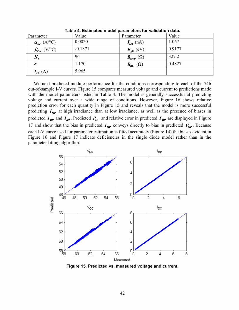
Table 4. Estimated model parameters for validation data. Parameter Value Parameter Value

(A/°C) 0.0020 (nA) 1.067 (V/°C) -0.1871 (eV) 0.9177

96 (Ω) 327.2 1.170 (Ω) 0.4827

(A) 5.965 We next predicted module performance for the conditions corresponding to each of the 746

out-of-sample I-V curves. Figure 15 compares measured voltage and current to predictions made with the model parameters listed in Table 4. The model is generally successful at predicting voltage and current over a wide range of conditions. However, Figure 16 shows relative prediction error for each quantity in Figure 15 and reveals that the model is more successful predicting at high irradiance than at low irradiance, as well as the presence of biases in predicted and . Predicted and relative error in predicted are displayed in Figure 17 and show that the bias in predicted conveys directly to bias in predicted . Because each I-V curve used for parameter estimation is fitted accurately (Figure 14) the biases evident in Figure 16 and Figure 17 indicate deficiencies in the single diode model rather than in the parameter fitting algorithm.

Figure 15. Predicted vs. measured voltage and current.

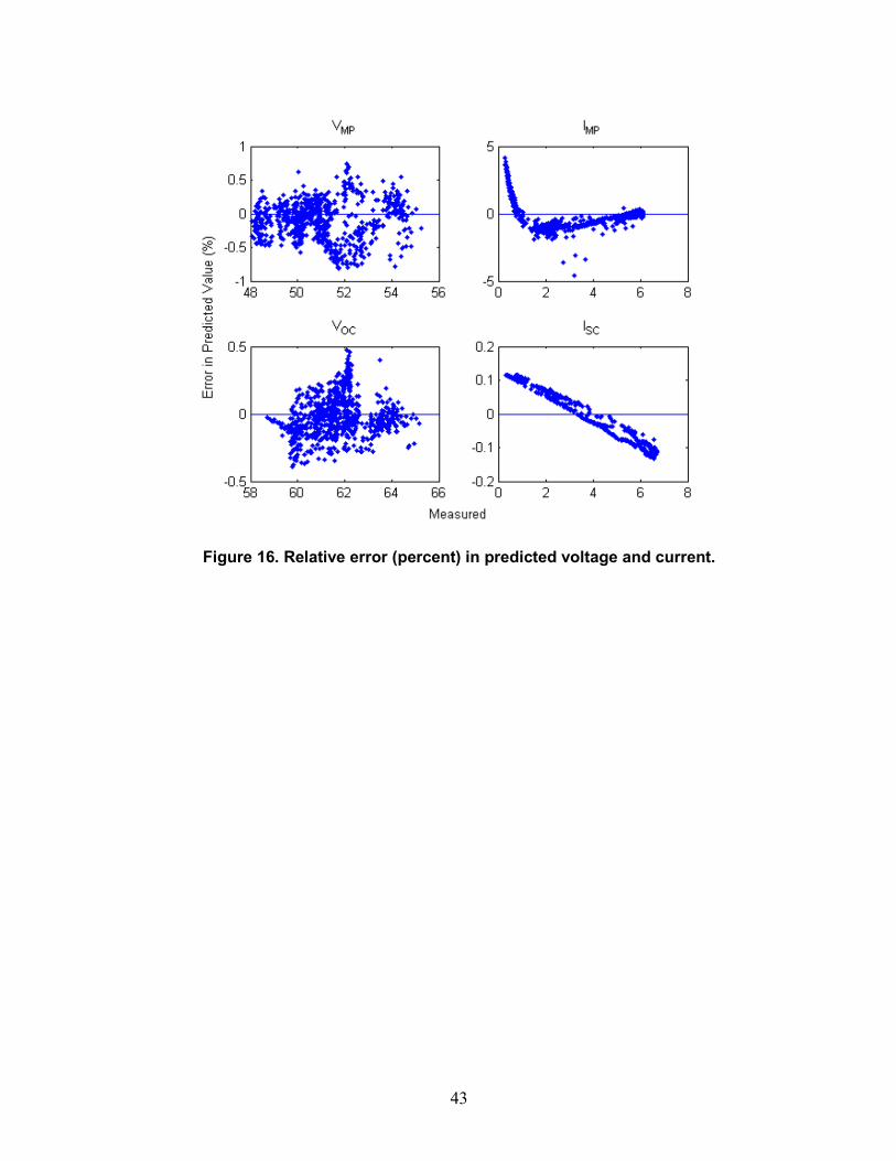
43

Figure 16. Relative error (percent) in predicted voltage and current.

44

0 50 100 150 200 250 300 3500

50

100

150

200

250

300

350

Measured PMP

(W)

Pre

dict

ed P

MP (W

)

0 50 100 150 200 250 300 350-5

-4

-3

-2

-1

0

1

2

3

4

5

Measured PMP

(W)

Erro

r in

Pre

dict

ed P

MP (%

)

Figure 17. Predicted vs. measured power and relative error in predicted power.

45

6. SUMMARY We have presented a new method for estimating parameters for single diode models,

illustrated by application to the single diode model specified in [2]. The method requires prior determination of module temperature coefficients for SCI and OCV and a set of I-V curves measured across a range of effective irradiance and cell temperature. The method first estimates the diode factor from measured OCV for a set of I-V curves, applies an iterative procedure to obtain values for LI , OI , SHR , and SR for each I-V curve, and finally, obtains parameters for the single diode model by a series of regressions.

We applied our method to recover parameters from I-V curves that were computed from several assumed sets of parameters for a single diode model to verify the method’s robustness. Being a sequential estimation algorithm, values for LI , OI , SHR , and SR for each fitted I-V curve are conditional on the value for the diode factor n . As demonstrated in Section 5.1, small errors in the recovered diode factor can result in significant differences in the values for the other parameters. The diode factor is estimated using a linear relationship (Eq. (22)) which is an approximation derived from the single diode equation (see Appendix D). We have observed that the other parameters for an I-V curve are quite sensitive to small changes in the diode factor. Consequently our method’s robustness may be improved by additional refinement of the technique for recovering the diode factor.

Our method involves numerical convergence at a number of steps. However, the initial values for the optimizations are not selected with randomness, and hence, subject to variation in machine precision and software (e.g., Matlab versions) we believe our method to be reliable.

Having outlined the method in detail we believe it to be accessible to one with an adequate mathematical and engineering background. However, we believe that the method, as described in this report, yet offers opportunities for simplification. For example, the initial estimate of SHR requires a fairly involved set of calculations (i.e., coordinate transformations, spline fitting and numerical integration) yet the initial estimate of SHR is later replaced with an updated value (see Section 4.2 Step 3c). Consequently, a less accurate initial estimate obtained by a simpler process may be just as good. We tested some simpler methods, e.g., Eq. (8) (see Appendix E) and found that most of the resulting values led to suitable values for all parameters. However the alternative methods also increased somewhat the number of I-V curves for which the parameter estimation failed and so we have retained the more complicated technique. We view the complexity involved in the initial estimate of SHR as indicating an opportunity to improve our algorithm.

46

47

7. REFERENCES

1. Mermoud, A. and T. Lejeune. Performance Assessment Of A Simulation Model For Pv Modules Of Any Available Technology. in 25th European Photovoltaic Solar Energy Conference, 2010. Valencia, Spain.

2. De Soto, W., S.A. Klein, and W.A. Beckman, Improvement and validation of a model for photovoltaic array performance. Solar Energy, 2006. 80(1): p. 78-88.

3. Gray, J.L., The Physics of the Solar Cell, in Handbook of Photovoltaic Science and Engineering, A. Luque, Hegedus, S., Editor. 2011, John Wiley and Sons.

4. Dobos, A., An Improved Coefficient Calculator for the California Energy Commission 6 Parameter Photovoltaic Module Model. Journal of Solar Energy Engineering, 2012. 134(2).

5. Duffie, J.A. and W.A. Beckman, Solar Engineering of Thermal Processes 2006: Wiley. 6. Ortiz-Conde, A., F.J. García Sánchez, and J. Muci, New method to extract the model

parameters of solar cells from the explicit analytic solutions of their illuminated I–V characteristics. Solar Energy Materials and Solar Cells, 2006. 90(3): p. 352-361.

7. Tian, H., et al., A cell-to-module-to-array detailed model for photovoltaic panels. Solar Energy, 2012. 86(9): p. 2695-2706.

8. Chan, D.S.H. and J.C.H. Phang, Analytical methods for the extraction of solar-cell single- and double-diode model parameters from I-V characteristics. Electron Devices, IEEE Transactions on, 1987. 34(2): p. 286-293.

9. Karmalkar, S. and S. Haneefa, A Physically Based Explicit Model of a Solar Cell for Simple Design Calculations. Electron Device Letters, IEEE, 2008. 29(5): p. 449-451.

10. Bonanno, F., et al., A radial basis function neural network based approach for the electrical characteristics estimation of a photovoltaic module. Applied Energy, 2012. 97(0): p. 956-961.

11. Farivar, G. and B. Asaei. Photovoltaic module single diode model parameters extraction based on manufacturer datasheet parameters. in Power and Energy (PECon), 2010 IEEE International Conference on, 2010.

12. Kim, W. and W. Choi, A novel parameter extraction method for the one-diode solar cell model. Solar Energy, 2010. 84(6): p. 1008-1019.

13. Phang, J.C.H., D.S.H. Chan, and J.R. Phillips, Accurate analytical method for the extraction of solar cell model parameters. Electronics Letters, 1984. 20(10): p. 406-408.

14. Dallago, E., D. Finarelli, and P. Merhej, Method based on single variable to evaluate all parameters of solar cells. Electronics Letters, 2010. 46(14): p. 1022-1024.

15. Ishibashi, K.I., Y. Kimura, and M. Niwano, An extensively valid and stable method for derivation of all parameters of a solar cell from a single current-voltage characteristic. Journal of Applied Physics, 2008. 103(9).

16. Datta, S.K., et al., An improved technique for the determination of solar cell parameters. Solid-State Electronics, 1992. 35(11): p. 1667-1673.

17. El-Naggar, K.M., et al., Simulated Annealing algorithm for photovoltaic parameters identification. Solar Energy, 2012. 86(1): p. 266-274.

18. Macabebe, E.Q.B., C.J. Sheppard, and E.E. van Dyk, Parameter extraction from I–V characteristics of PV devices. Solar Energy, 2011. 85(1): p. 12-18.

19. Chegaar, M., G. Azzouzi, and P. Mialhe, Simple parameter extraction method for illuminated solar cells. Solid-State Electronics, 2006. 50(7–8): p. 1234-1237.

48

20. Caracciolo, F., et al., Single-Variable Optimization Method for Evaluating Solar Cell and Solar Module Parameters. Photovoltaics, IEEE Journal of, 2012. 2(2): p. 173-180.

21. Peng, L., et al., A new method for determining the characteristics of solar cells. Journal of Power Sources, 2013. 227(0): p. 131-136.

22. Chen, Y., et al., Parameters extraction from commercial solar cells I–V characteristics and shunt analysis. Applied Energy, 2011. 88(6): p. 2239-2244.

23. Corless, R.M., et al., On the Lambert W Function in Advances in Computational Mathematics. 1996. p. 329-359.

24. Ortiz-Conde, A., F.J. Garcıa Sánchez, and J. Muci, Exact analytical solutions of the forward non-ideal diode equation with series and shunt parasitic resistances. Solid-State Electronics, 2000. 44(10): p. 1861-1864.

25. Jain, A. and A. Kapoor, Exact analytical solutions of the parameters of real solar cells using Lambert W-function. Solar Energy Materials and Solar Cells, 2004. 81(2): p. 269-277.

26. Barry, D.A., S.J. Barry, and P.J. Culligan-Hensley, Algorithm-743 - Wapr - a Fortran Routine for Calculating Real Values of the W-Function. ACM Transactions on Mathematical Software, 1995. 21(2): p. 172-181.

27. (IEC), I.E.C., 60891 Ed. 2.0: Photovoltaic devices - Procedures for temperature and irradiance corrections to measured I-V characteristics, 2010, IEC.

28. Hansen, C., et al. Parameter Uncertainty in the Sandia Array Performance Model for Flat-Plate Crystalline Silicon Modules. in 37th IEEE Photovoltaics Specialists Conference, 2011. Seattle, WA.

29. Hansen, C., D. Riley, and M. Jaramillo. Calibration of the Sandia Array Performance Model Using Indoor Measurements in IEEE Photovoltaic Specialists Conference, 2012. Austin, TX.

30. King, D.L., E.E. Boyson, and J.A. Kratochvil, Photovoltaic Array Performance Model, SAND2004-3535, Sandia National Laboratories, Albuquerque, NM, 2004.

31. Hansen, C., A. Luketa-Hanlin, and J.S. Stein. Sensitivity Of Single Diode Models For Photovoltaic Modules To Method Used For Parameter Estimation. in 28th European Photovoltaic Solar Energy Conference, 2013. Paris, FR.

32. Burden, R.L. and J.D. Faires, Numerical analysis. 4th ed. The Prindle, Weber, and Schmidt series in mathematics. 1989, Boston: PWS-KENT Pub. Co. xv, 729 p.

33. Bowen, M.K. and R. Smith, Derivative formulae and errors for non-uniformly spaced points. Proceedings of the Royal Society A: Mathematical, Physical and Engineering Science, 2005. 461(2059): p. 1975-1997.

34. ASTM, Standard Tables for Reference Solar Spetral Irradiances: Direct Normal and Hemispherical on 37° Tilted Surface, 2012, ASTM International.

35. (IEC), I.E.C., 61853-1 Ed. 1.0: Photovoltaic (PV) module performance testing and energy rating - Part I: Irradiance and temperature performance measurements and power rating, 2011.

36. (IEC), I.E.C., 60904-5 Ed. 2.0: Photovoltaic devices - Part 5: Determination of the equivalent cell temperature (ECT) of photovoltaic (PV) devices by the open-circuit voltage method, 2011.

37. Næs, T. and B.-H. Mevik, Understanding the collinearity problem in regression and discriminant analysis. Journal of Chemometrics, 2001. 15(4): p. 413-426.

49

38. Schumaker, L., On Shape Preserving Quadratic Spline Interpolation. SIAM Journal on Numerical Analysis, 1983. 20(4): p. 854-864.

50

51

APPENDIX A: EXPLICIT SOLUTION OF THE SINGLE DIODE EQUATION

Lambert’s W function is the solution ( )W W x= of the equation ( )expx W W= . An equation

of the form

ax bp cx d+ = + (A1)

can be transformed by the substitution

adt axc

− = + (A2)

to

adbt catp p

c−

= − (A3)

By the definition of Lambert’s W, we obtain

ln

ln

adbcaW p p

ct

p

− − = (A4)

which leads to a solution of Eq. (A1) in terms of Lambert’s W function:

1 lnln

adbca p dx W p

a p c c−

= − − −

(A5)

Considering ( )I I V= and applying this process to the single diode equation (Eq. (1)), we obtain

( )

exp 1

exp

S SL O

th SH

L O SHS SH S

th th O SH O SH

V IR V IRI I InV R

I I R VR R RVI InV nV I R I R

+ += − − −

+ − +

+ = − +

(A6)

which after using Eq. (A5) simplifies to Eq. (9) A similar process yields Eq. (10).

52

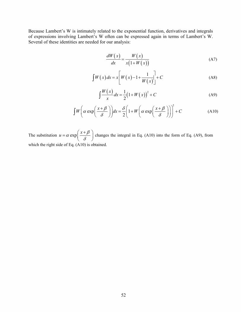
Because Lambert’s W is intimately related to the exponential function, derivatives and integrals of expressions involving Lambert’s W often can be expressed again in terms of Lambert’s W. Several of these identities are needed for our analysis:

( ) ( )

( )( )1dW x W x

dx x W x=

+ (A7)

( ) ( ) ( )11W x dx x W x C

W x

= − + +

∫ (A8)

( ) ( )( )21 1

2W x

dx W x Cx

= + +∫ (A9)

2

exp 1 exp2

x xW dx W Cβ d βα αd d

+ + = + + ∫ (A10)

The substitution exp xu βαd+ =

changes the integral in Eq. (A10) into the form of Eq. (A9), from

which the right side of Eq. (A10) is obtained.

53

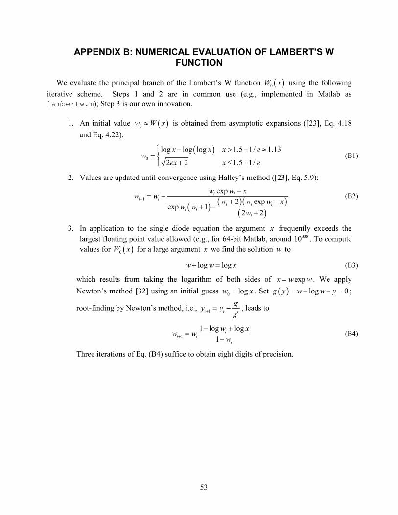
APPENDIX B: NUMERICAL EVALUATION OF LAMBERT’S W FUNCTION

We evaluate the principal branch of the Lambert’s W function ( )0W x using the following

iterative scheme. Steps 1 and 2 are in common use (e.g., implemented in Matlab as lambertw.m); Step 3 is our own innovation.

1. An initial value ( )0w W x≈ is obtained from asymptotic expansions ([23], Eq. 4.18

and Eq. 4.22):

( )

0

log log log 1.5 1/ 1.13

2 2 1.5 1/

x x x ew

ex x e

− > − ≈= + ≤ −

(B1)

2. Values are updated until convergence using Halley’s method ([23], Eq. 5.9):

( ) ( )( )

( )1

exp2 exp

exp 12 2

i ii i

i i ii i

i

w w xw ww w w x

w ww

+

−= −

+ −+ −

+

(B2)

3. In application to the single diode equation the argument x frequently exceeds the largest floating point value allowed (e.g., for 64-bit Matlab, around 30810 . To compute values for ( )0W x for a large argument x we find the solution w to

log logw w x+ = (B3)

which results from taking the logarithm of both sides of expx w w= . We apply Newton’s method [32] using an initial guess 0 logw x= . Set ( ) log 0g y w w y= + − = ;

root-finding by Newton’s method, i.e., 1i igy yg+ = −′, leads to

11 log log

1i

i ii

w xw ww+

− +=

+ (B4)

Three iterations of Eq. (B4) suffice to obtain eight digits of precision.

54

APPENDIX C: I-V CURVE FITTING USING THE CO-CONTENT INTEGRAL

C.1. Relationship between the co-content and the five parameters. Here we define the co-content integral and demonstrate the relationship between the co-

content integral and the parameters for the single diode equation (Eq. (1)). This relationship was first published by [6]; we provide here additional details regarding the derivation of the equations presented in [6] and comment on several challenges presented by the method described in [6]. We differ from [6] by setting the sign on current flow as indicated Figure 1 to obtain Eq. (1); [6] reverses the sign on the current flow.

Define the co-content ( )CC CC V= by

( ) ( )( )0

V

SCCC V I I dη η= −∫ (C1)

In [6] the definition is given as ( ) ( )( )0

V

SCCC V I I dη η= −∫ because the single diode equation is

also given in [6] using active rather than passive sign convention. Figure C1 illustrates the co-content function.

Figure C1. Illustration of co-content integral.

55

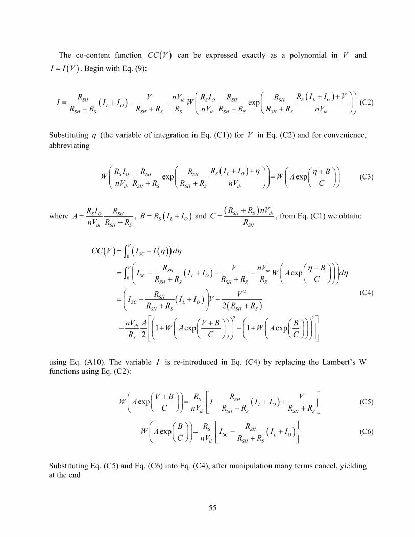
The co-content function ( )CC V can be expressed exactly as a polynomial in V and

( )I I V= . Begin with Eq. (9):

( ) ( )exp S L OSH th S O SH SHL O

SH S SH S S th SH S SH S th

R I I VR nV R I R RVI I I WR R R R R nV R R R R nV

+ + = + − − + + + +

(C2)

Substituting η (the variable of integration in Eq. (C1)) for V in Eq. (C2) and for convenience, abbreviating

( )exp expS L OS O SH SH

th SH S SH S th

R I IR I R R BW W AnV R R R R nV C

η η + + + = + + (C3)

where S O SH

th SH S

R I RAnV R R

=+

, ( )S L OB R I I= + and ( )SH S th

SH

R R nVC

R+

= , from Eq. (C1) we obtain:

( ) ( )( )

( )

( ) ( )

0

0

2

2 2

exp

2

1 exp 1 exp2

V

SC

V SH thSC L O

SH S SH S S

SHSC L O

SH S SH S

th

S

CC V I I d

R nVV BI I I W A dR R R R R C

R VI I I VR R R R

nV A V B BW A W AR C C

η η

η η

= −

+ = − + − − + +

= − + − + + + − + − +

∫

∫ (C4)

using Eq. (A10). The variable I is re-introduced in Eq. (C4) by replacing the Lambert’s W functions using Eq. (C2):

( )exp S SHL O

th SH S SH S

R RV B VW A I I IC nV R R R R

+ = − + + + + (C5)

( )exp S SHSC L O

th SH S

R RBW A I I IC nV R R

= − + + (C6)

Substituting Eq. (C5) and Eq. (C6) into Eq. (C4), after manipulation many terms cancel, yielding at the end

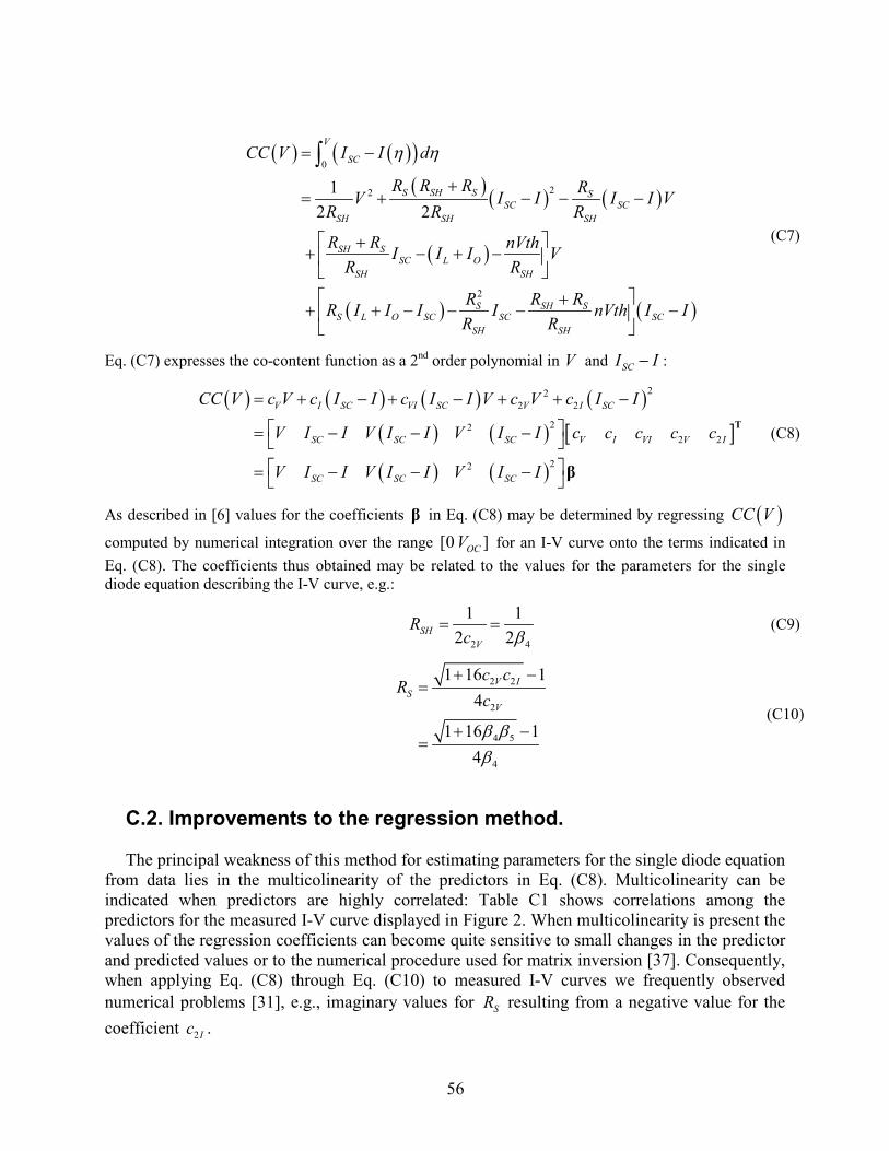
56

( ) ( )( )( ) ( ) ( )

( )

( ) ( )

0

22

2

12 2

V

SC

S SH S SSC SC

SH SH SH

SH SSC L O

SH SH

S SH SS L O SC SC SC

SH SH

CC V I I d

R R R RV I I I I VR R R

R R nVthI I I VR R

R R RR I I I I nVth I IR R

η η= −

+= + − − −

++ − + − +

+ + − − − −

∫

(C7)

Eq. (C7) expresses the co-content function as a 2nd order polynomial in V and SCI I− :

( ) ( ) ( ) ( )( ) ( ) [ ]

( ) ( )

222 2

222 2

22

V I SC VI SC V I SC

SC SC SC V I VI V I

SC SC SC

CC V c V c I I c I I V c V c I I

V I I V I I V I I c c c c c

V I I V I I V I I

= + − + − + + −

= − − − = − − −

T

β

(C8)

As described in [6] values for the coefficients β in Eq. (C8) may be determined by regressing ( )CC V

computed by numerical integration over the range [0 ]OCV for an I-V curve onto the terms indicated in Eq. (C8). The coefficients thus obtained may be related to the values for the parameters for the single diode equation describing the I-V curve, e.g.:

2 4

1 12 2SH

V

Rc β

= = (C9)

2 2

2

4 5

4

1 16 14

1 16 14

V IS

V

c cR

c

β ββ

+ −=

+ −=

(C10)

C.2. Improvements to the regression method. The principal weakness of this method for estimating parameters for the single diode equation

from data lies in the multicolinearity of the predictors in Eq. (C8). Multicolinearity can be indicated when predictors are highly correlated: Table C1 shows correlations among the predictors for the measured I-V curve displayed in Figure 2. When multicolinearity is present the values of the regression coefficients can become quite sensitive to small changes in the predictor and predicted values or to the numerical procedure used for matrix inversion [37]. Consequently, when applying Eq. (C8) through Eq. (C10) to measured I-V curves we frequently observed numerical problems [31], e.g., imaginary values for SR resulting from a negative value for the coefficient 2Ic .

57

Table C1. Correlation coefficients for predictors in Eq. C8.

V SCI I− ( )SCV I I− 2V ( )2SCI I−

V 1.000 0.626 0.609 0.968 0.484

SCI I− 0.626 1.000 0.999 0.750 0.954

( )SCV I I− 0.609 0.999 1.000 0.734 0.964 2V 0.968 0.750 0.734 1.000 0.601

( )2SCI I− 0.484 0.954 0.964 0.601 1.000

We observed that the coefficients in Eq. (C8) are quite sensitive to small deviations in ( )CC V resulting from the numerical integration procedures. For example, a simple trapezoid

rule applied to compute ( )CC V will produce biased values because the I-V curve is generally concave downward (Figure C1), and hence the values computed by a trapezoid rule will be negatively biased. The biased values in turn affect the coefficients indicated in Eq. (C8).

Multicolinearity among predictors may be remedied by a number of different techniques. We attempted several, including: standardizing the predictors, dropping predictors from the model, ridge regression, and principal components transformations involving several or all of the predictors. Among these methods we found that a principal components transformation of the predictors V and SCI I− yielded more reliable results than other methods, as judged by the agreement between the fitted single diode equation and the data, and the frequency of obtaining reasonable parameter values from I-V curve data without visible flaws (e.g., increasing current with increasing voltage). However, none of the methods we explored resulted in reasonable coefficient values for most I-V curves for each of a set of modules with diverse characteristics.

We use a modified version of the approach from [6] only to obtain an initial estimate of SHR . We modified the method in [6] to include the following steps:

1. Fit a quadratic spline ( )S V to the I-V curve data ( ), , 0, ,k kV I k N= , where

( ) ( )0 0, 0, SCV I I= and ( ) ( ), ,0N N OCV I V= using a technique [38] that preserves the monotonicity and convexity expected in the I-V curve. Ideally the data describing a measured I-V curve are monotonic decreasing and concave downward. Compute

( )k kCC CC V= by exact integration of the quadratic spline ( )S V fitted in Step 1. Because the spline fit is more sensitive to data variation at the ends of the I-V curve data (i.e, near SCI and OCV , e.g., for 0 5k≤ < and 5N k N− < ≤ ) a trapezoid rule is used to compute kCC for these intervals.

2. Standardize the predictors V and SCII I I= − by shifting and scaling to obtain

k V

k

V

VV µσ−

= (C11)

and

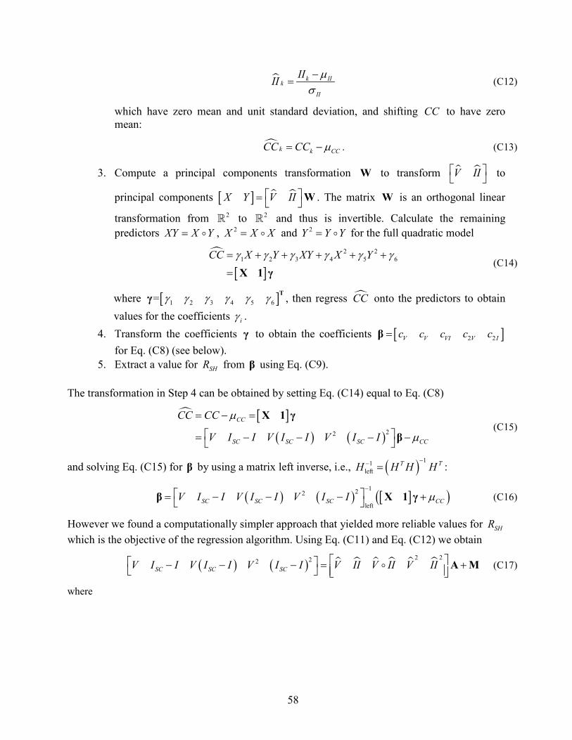
58

k II

k

II

IIII µσ−

= (C12)

which have zero mean and unit standard deviation, and shifting CC to have zero mean:

k k CCCC CC µ= − . (C13)

3. Compute a principal components transformation W to transform V II to

principal components [ ] X Y V II = W . The matrix W is an orthogonal linear

transformation from 2 to 2

and thus is invertible. Calculate the remaining predictors XY X Y= , 2X X X= and 2Y Y Y= for the full quadratic model

[ ]

2 21 2 3 4 5 6CC X Y XY X Yγ γ γ γ γ γ= + + + + +

= X 1 γ (C14)

where [ ]1 2 3 4 5 6= γ γ γ γ γ γ Tγ , then regress CC onto the predictors to obtain values for the coefficients iγ .

4. Transform the coefficients γ to obtain the coefficients [ ]2 2V V VI V Ic c c c c=β for Eq. (C8) (see below).

5. Extract a value for SHR from β using Eq. (C9). The transformation in Step 4 can be obtained by setting Eq. (C14) equal to Eq. (C8)

[ ]

( ) ( )22

CC

SC SC SC CC

CC CC

V I I V I I V I I

µ

µ

= − =

= − − − −

X 1 γ

β (C15)

and solving Eq. (C15) for β by using a matrix left inverse, i.e., ( ) 11left

T TH H H H−− = :

( ) ( ) [ ]( )122

leftSC SC SC CCV I I V I I V I I µ

− = − − − + β X 1 γ (C16)

However we found a computationally simpler approach that yielded more reliable values for SHR which is the objective of the regression algorithm. Using Eq. (C11) and Eq. (C12) we obtain

( ) ( )

2 222SC SC SCV I I V I I V I I V II V II V II − − − = +

A M (C17)

where

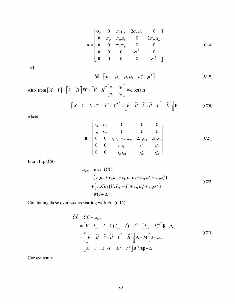
59

2

2

0 2 00 0 20 0 0 00 0 0 00 0 0 0

V V II V V

II II V II II

V II

V

II

σ σ µ σ µσ σ µ σ µ

σ σσ

σ

=

A (C18)

and

2 2V I V I V Iµ µ µ µ µ µ = M (C19)

Also, from [ ]

11 12

21 22

r rX Y V II V II

r r = =

W we obtain

2 22 2X Y X T X Y V II V II V II = B (C20)

where

11 12

21 22

11 22 12 21 11 21 12 222 2

11 12 11 122 2

21 22 21 22

0 0 00 0 0

0 0 2 20 00 0

r rr r

r r r r r r r rr r r rr r r r

= +

B (C21)

From Eq. (C8),

( )

( )( )

2 22 2

2 22 2

mean( )

,

CC

V V V V VI V I V V I I

VI SC V V I II

CC

c c c c c

c Cov V I I c c

µ

µ µ µ µ µ µ

σ σ

=

= + + + +

+ − + +

= + ∆Mβ

(C22)

Combining these expressions starting with Eq. (C15)

( ) ( )

22

2 2

2 2 1

CC

SC SC SC CC

CC

CC CC

V I I V I I V I I

V II V II V II

X Y X T X Y

µ

µ

µ

−

= −

= − − − − = + − = − ∆

β

A M β

B Aβ

(C23)

Consequently

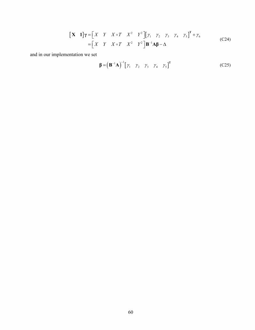
60

[ ] [ ]2 2

1 2 3 4 5 6

2 2 1

X Y X T X Y

X Y X T X Y

γ γ γ γ γ γ−

= + = − ∆

TX 1 γ

B Aβ

(C24)

and in our implementation we set

( ) [ ]111 2 3 4 5γ γ γ γ γ

−−= Tβ B A (C25)

61

APPENDIX D: ASYMPTOTIC ANALYSIS FOR VOC

Here, we show that Eq. (D1), relating OCV to ( )0ln E E , derives from a simplification to the

single diode equation.

( )0 0lnOC OC thV V nV E E− ≈ (D1)

Denote reference conditions and parameters at reference conditions by the subscript 0~ . From Eq. (10) we have

( ) ( )exp L O SHO SHOC L O SH th

th th

I I RI RV I I R nV WnV nV

+ = + −

(D2)

and at reference conditions:

( ) ( )0 0 00 00 0 0 0 0

0 0

exp L O SHO SHOC L O SH th

th th

I I RI RV I I R nV WnV nV

+ = + −

(D3)

The argument of the W function in Eq. (D2) is extremely large due to the factor ( )exp L O SH

th

I I RnV+

, e.g., ( )6A 200exp exp 5501.1 2V× Ω = ×

which results when substituting

coefficient values representative of a 72-cell cSi module. Therefore we may approximate ( ) ln ln ln lnW x x x x− ≈− [23] and obtain from Eq. (D2)

( ) ( )ln

ln

L O SHO SHOC L O SH th

th th

O SHth

th

I I RI RV I I R nVnV nV

I RnVnV

+ ≈ + − +

= −

(D4)

and from Eq. (D3)

0 00 0

0

ln O SHOC th

th

I RV nVnV

≈ −

(D5)

Setting 0CT T= (i.e., the cells are at the selected reference temperature), we have 0th thV V= and

0O OI I≈ (from Eq. (3)) so Eq. (D4) and Eq. (D5) lead to

62

0 0 00 0 0

0 0

00

00

ln ln

ln

ln

O SH O SHOC OC th th

th th

SHth

SH

th

I R I RV V nV nVnV nV

RnVR

EnVE

− ≈ − +

=

=

(D6)

where the last line results from Eq. (5): 0 0SH SHR R E E= . Eq. (5) is specific to the single diode model in [2], and the relationship in Eq. (D1) should also be established for other single diode models (e.g., PVsyst [1]) that use different relationships between SHR and E .

63

APPENDIX E: EVALUATION OF APPROXIMATIONS IN THE SINGLE DIODE EQUATION

We considered several simplifications to the single diode equation which are obtained by

substituting approximations for LI or SHR in order to reduce the number of parameters to be estimated. We found that, in each case considered, the approximations led to unreasonably small values for SR .

Approximations for LI . It is common to approximate LI as L SCI I≈ or as ( )1L S SH SCI R R I≈ + either of which

effectively replace the unknown parameter LI with the measured value of SCI . However, these substitutions are analytically equivalent to assuming that 0SR = in the first case or that SR is unreasonably small or negative in the second case. Consequently we do not recommend use of these simplifications.

Eq. (10) may be re-arranged to obtain an expression for SR at SCI I= :

( )exp L O SC SHL O SC O SH

S SH thSC th th

I I I RI I I I RR R nV WI nV nV

+ − + −= −

(E1)

Substituting 1 SL SC

SH

RI IR

= +

leads to

( ) ( )( )exp

exp

exp

S SH SC O SHS SH SC O th O SHS SH

SC SC th th

S SC SH O th O SH S SC SH O

SC SC th th

SH O th O SH S SC SH OS

SC SC th th

R R I I RR R I I nV I RR R WI I nV nV

R I R I nV I R R I R IWI I nV nV

R I nV I R R I R IR WI I nV nV

++ = −

+ += −

+= + −

(E2)

and in turn

expSH O O SH S SC SH O

th th th

R I I R R I R IWnV nV nV

+=

(E3)

Applying the definition of Lambert’s W function to Eq. (E3) obtains

exp expSH O SH O O SH S SC SH O

th th th th

R I R I I R R I R InV nV nV nV

+=

(E4)

which implies 0S SCR I = and in turn 0SR = .

64

Setting L SCI I≈ leads to unreasonably small values for SR . Substituting L SCI I= into the single diode equation at SCI I= (Eq. (1)):

0 exp SC S SC SO O

th SH

I R I RI InV R

= − −

(E5)

leads to

1 expSC SCS S

SH O th

I IR RR I nV

− + =

(E6)

which can be solved for SR using the transformation indicated by Eq. (A2):

expO SH O SHS

th th

I R I RR WnV nV

=

(E7)

Reasonable values for OI and SHR lead to 8 3 510 10 10O SHI R − −× =− which in turn results in

( )5 5exp ~ 10 1 ~ 10O SH O SHS

th th

I R I RR W WnV nV

− − = ×

which is far too small to be reasonable.

Approximation for SHR . If we approximate

SC

SHI I

dVRdI =

≈ − (E8)

and impose the resulting value on the estimates of the remaining three parameters (i.e., LI , OI and SR ) for an I-V curve, we find that the resulting value for SR will be orders of magnitude smaller than is credible. From Eq. (10)

( ) ( )

( ) ( )

exp L O SHO SHL O SH S th

th th

L O SH S th

I I I RI RV I I I R IR nV WnV nV

I I I R IR nV W ψ

+ − = + − − − = + − − −

(E9)

where

( )exp L O SHO SH

th th

I I I RI RnV nV

ψ+ −

=

(E10)

we compute

( )( )( )1SH S SH

WdV R R RdI W

ψψ ψ

= − − ++

(E11)

65

using Eq. (A7). Substituting

( )( )( ) ( )( )( )1

SC

SHI I

SCSH S SH

SC SC

dVRdI

W IR R R

I W I

ψ

ψ ψ

=

= −

= + −+

(E12)

leads to

( )

( )( )( )( )( )1SCSH

SSC SC

W IRRI W I

ψψ ψ

=+

(E13)

For a reasonable module,

( ) ( )

( )

8 3 1 3

5

16

exp

10 10 10 10~ exp2 2

~ 10 exp 50

~ 10

L O SHO SHSC

th th

I I I RI RInV nV

ψ

− −

−

+ − =

(E14)

which implies that

3

16

10~10SR (E15)

which is far too small to be credible. Figure E2 compares estimates of SHR obtained using the regression method (i.e., [6] with our

improvements) to those obtained using the common approximation in Eq. (E8). In this case, the derivative required in Eq. (E8) is computed by averaging the numerical derivatives obtained at each voltage point using [33] for 0.5 OCV V< . Note that the number of I-V curves with reasonable values for SHR are slightly fewer. The estimates from Eq. (E8) are systematically greater but are likely adequate as initial values for the updating algorithm described in Section 4.2, Step 3. Consequently the advantage of the more complex regression method is to more reliably obtain adequate initial values.

66

0 200 400 600 800 1000 12002

2.5

3

3.5

4

4.5

Effective irradiance (W/m2)

log 10

RS

H (R

SH

in Ω

)

Regression method (947 values)Eq. (E8) (942 values)

Figure E2. Initial estimates of RSH using different methods.

67

Distribution 1 MS0899 Technical Library 9536 (electronic copy) 1 MS0161 Legal Technology Transfer Center 11500