Parameter estimation for Parameter estimation for nonlinear models: Numerical nonlinear models: Numerical

approaches to solving the inverse approaches to solving the inverse problemproblem

Lecture 10Lecture 10 03/25/200803/25/2008

Sven Zenker

Review: Multiple Shooting homeworkReview: Multiple Shooting homeworkMethod of Multipliers:Method of Multipliers:

function [x, function [x, lastlambdalastlambda] = ] = mom(fhmom(fh, x0, , x0, terminationNormterminationNorm, , maxitermaxiter, lb, , lb, ubub))% minimize function f: % minimize function f: R^nR^n --> R > R s.ts.t. g: . g: R^nR^n --> > R^mR^m = 0 using Method of= 0 using Method of% Multipliers% Multipliers% function [% function [fxfx, , gradfgradf, , hxhx, , jachxjachx] = ] = fh(xfh(x))% % terminationNormterminationNorm = 1E= 1E--5; % terminate when constraint violation < than this5; % terminate when constraint violation < than this% % maxitermaxiter = 25;= 25;

beta = 5; % factor by which to increase c in each iterationbeta = 5; % factor by which to increase c in each iteration% first evaluation, find out dimensions% first evaluation, find out dimensions[[fxfx, , gradfgradf, , hxhx, , jachxjachx] = fh(x0)] = fh(x0)% initialization% initializationdimhdimh = = length(hxlength(hx); ); c = 1;c = 1;lambda = lambda = zeros(dimhzeros(dimh, 1); % 0 as initial guess for Lagrange multiplier, 1); % 0 as initial guess for Lagrange multiplierlastlambdalastlambda = lambda;= lambda;x = x0;x = x0;iteriter = 0;= 0;

opts = opts = optimset('Displayoptimset('Display', '', 'IterIter', '', 'GradObjGradObj', 'on', '', 'on', 'MaxIterMaxIter', 50);', 50);

while(norm(hxwhile(norm(hx) > ) > terminationNormterminationNorm && && iteriter < < maxitermaxiter))if if isempty(lbisempty(lb) && ) && isempty(ubisempty(ub))

[x, [x, fxfx] = ] = fminunc(@(thexfminunc(@(thex) ) L(thexL(thex, c, lambda), x, opts); % minimize augmented , c, lambda), x, opts); % minimize augmented LagrangianLagrangian with current parameter valueswith current parameter valueselseelse

[x, [x, fxfx] = ] = fmincon(@(thexfmincon(@(thex) ) L(thexL(thex, c, lambda), x, [], [], [], [], lb, , c, lambda), x, [], [], [], [], lb, ubub, [], opts); % minimize augmented , [], opts); % minimize augmented LagrangianLagrangian with current parameter valueswith current parameter valuesendend[[fxfx, , jacfxjacfx, , hxhx, , jachxjachx] = ] = fh(xfh(x); % find ); % find contraintcontraint valuesvaluesdisp(sprintf('Iterationdisp(sprintf('Iteration %d: %d: GradObjGradObj c=%d, c=%d, f(xf(x) = %d, ) = %d, norm(h(xnorm(h(x)) = %d', )) = %d', iteriter, c, , c, fxfx, , norm(hxnorm(hx)));)));lastlambdalastlambda = lambda;= lambda;lambda = lambda = lambdalambda + c*+ c*hxhx; % Method of Multipliers ; % Method of Multipliers LangrangeLangrange Multiplier Multiplier updataupdatac = beta * c; % increase penalty weightc = beta * c; % increase penalty weightiteriter = iter+1;= iter+1;

endend

function [Lx, function [Lx, gradLxgradLx] = ] = L(xL(x, c, lambda), c, lambda)% augmented % augmented LagrangianLagrangian with quadratic penalty termwith quadratic penalty term[[fxfx, , gradfgradf, , hxhx, , jachxjachx] = ] = fh(xfh(x););Lx = Lx = fxfx + lambda' * + lambda' * hxhx + c/2*+ c/2*hxhx'*'*hxhx;;gradLxgradLx = = gradfgradf + (lambda' * + (lambda' * jachxjachx)' + c * )' + c * jachxjachx' * ' * hxhx;;

endend

endend

Review: Multiple Shooting homeworkReview: Multiple Shooting homeworkMethod of Multipliers, initialization:Method of Multipliers, initialization:

function [x, function [x, lastlambdalastlambda] = ] = mom(fhmom(fh, x0, , x0, terminationNormterminationNorm, , maxitermaxiter, lb, , lb, ubub))% minimize function f: % minimize function f: R^nR^n --> R > R s.ts.t. g: . g: R^nR^n --> > R^mR^m = 0 using Method of= 0 using Method of% Multipliers% Multipliers% function [% function [fxfx, , gradfgradf, , hxhx, , jachxjachx] = ] = fh(xfh(x))% % terminationNormterminationNorm = 1E= 1E--5; % terminate when constraint violation < than this5; % terminate when constraint violation < than this% % maxitermaxiter = 25;= 25;

beta = 5; % factor by which to increase c in each iterationbeta = 5; % factor by which to increase c in each iteration% first evaluation, find out dimensions% first evaluation, find out dimensions[[fxfx, , gradfgradf, , hxhx, , jachxjachx] = fh(x0)] = fh(x0)% initialization% initializationdimhdimh = = length(hxlength(hx); ); c = 1;c = 1;lambda = lambda = zeros(dimhzeros(dimh, 1); % 0 as initial guess for Lagrange multiplier, 1); % 0 as initial guess for Lagrange multiplierlastlambdalastlambda = lambda;= lambda;x = x0;x = x0;iteriter = 0;= 0;

opts = opts = optimset('Displayoptimset('Display', '', 'IterIter', '', 'GradObjGradObj', 'on', '', 'on', 'MaxIterMaxIter', 50);', 50);

Review: Multiple Shooting homeworkReview: Multiple Shooting homeworkMethod of Multipliers, main loop:Method of Multipliers, main loop:

while(norm(hxwhile(norm(hx) > ) > terminationNormterminationNorm && && iteriter < < maxitermaxiter))if if isempty(lbisempty(lb) && ) && isempty(ubisempty(ub))

[x, [x, fxfx] = ] = fminunc(@(thexfminunc(@(thex) ) L(thexL(thex, c, lambda), x, opts); % minimize , c, lambda), x, opts); % minimize augmented augmented LagrangianLagrangian with current parameter valueswith current parameter values

elseelse[x, [x, fxfx] = ] = fmincon(@(thexfmincon(@(thex) ) L(thexL(thex, c, lambda), x, [], [], [], [], lb, , c, lambda), x, [], [], [], [], lb, ubub, ,

[], opts); % minimize augmented [], opts); % minimize augmented LagrangianLagrangian with current parameter with current parameter valuesvalues

endend[[fxfx, , jacfxjacfx, , hxhx, , jachxjachx] = ] = fh(xfh(x); % find constraint values); % find constraint valuesdisp(sprintf('Iterationdisp(sprintf('Iteration %d: %d: GradObjGradObj c=%d, c=%d, f(xf(x) = %d, ) = %d, norm(h(xnorm(h(x)) = )) =

%d', %d', iteriter, c, , c, fxfx, , norm(hxnorm(hx)));)));lastlambdalastlambda = lambda;= lambda;lambda = lambda = lambdalambda + c*+ c*hxhx; % Method of Multipliers ; % Method of Multipliers LangrangeLangrange

Multiplier updateMultiplier updatec = beta * c; % increase penalty weightc = beta * c; % increase penalty weightiteriter = iter+1;= iter+1;

endend

Review: Multiple Shooting homeworkReview: Multiple Shooting homeworkMethod of Multipliers, objective function:Method of Multipliers, objective function:

function [Lx, function [Lx, gradLxgradLx] = ] = L(xL(x, c, lambda), c, lambda)% augmented % augmented LagrangianLagrangian with quadratic penalty termwith quadratic penalty term[[fxfx, , gradfgradf, , hxhx, , jachxjachx] = ] = fh(xfh(x););Lx = Lx = fxfx + lambda' * + lambda' * hxhx + c/2*+ c/2*hxhx'*'*hxhx;;gradLxgradLx = = gradfgradf + (lambda' * + (lambda' * jachxjachx)' + c * )' + c * jachxjachx' * ' * hxhx;;

endend

Multiple shooting: initialization and Multiple shooting: initialization and solutionsolution

function [opty0, function [opty0, optparsoptpars] = ] = multiShoot(tdatamultiShoot(tdata, data, , data, odesolodesol, p0, , p0, pLowerpLower, , pUpperpUpper, , nodeindicesnodeindices))

if nodeindices(1) ~= 1if nodeindices(1) ~= 1nodeindicesnodeindices = [= [nodeindicesnodeindices; 1];; 1];

endendnumNodesnumNodes = = length(nodeindiceslength(nodeindices););numDimnumDim = = size(datasize(data, 1); % data in column vectors, since we assume fully and direc, 1); % data in column vectors, since we assume fully and directly observed system, tly observed system,

equal to solution dimensionequal to solution dimensionnumObsnumObs = = size(datasize(data, 2);, 2);numParsnumPars = length(p0);= length(p0);

% initialize initial guesses for initial conditions% initialize initial guesses for initial conditionsicsics = = zeros(numDimzeros(numDim, , numNodesnumNodes););for i = 1:length(nodeindices)for i = 1:length(nodeindices)

icsics(:, i) = data(:, (:, i) = data(:, nodeindices(inodeindices(i));));endend% create initial guess vector% create initial guess vectorx0 = [x0 = [reshape(icsreshape(ics, [, [numNodesnumNodes* * numDimnumDim 1]); p0];1]); p0];% and run method of multipliers on this...% and run method of multipliers on this...

lb = [lb = [ones(numNodesones(numNodes * * numDimnumDim, 1) * , 1) * --InfInf; ; pLowerpLower]; % constrain parameters to be positive]; % constrain parameters to be positiveubub = [= [ones(numNodesones(numNodes * * numDimnumDim, 1) * , 1) * InfInf; ; pUpperpUpper]; % constrain parameters to be positive]; % constrain parameters to be positive

[x, lambda] = [x, lambda] = mom(@msObjFunctionmom(@msObjFunction, x0, 1E, x0, 1E--3, 25, lb, 3, 25, lb, ubub))

opty0 = x(1:numDim); % initial conditions for first interval = opty0 = x(1:numDim); % initial conditions for first interval = overall initial conditionsoverall initial conditionsoptparsoptpars = = x(numDimx(numDim*numNodes+1:end); % parameters*numNodes+1:end); % parameters

Multiple shooting: objective function Multiple shooting: objective function (1)(1)

function [function [fxfx, , gradfxgradfx, , hxhx, , jachxjachx] = ] = msObjFunction(xmsObjFunction(x))cicscics = reshape(x(1:numNodes*= reshape(x(1:numNodes*numDimnumDim), [), [numDimnumDim numNodesnumNodes]); % extract initial conditions ]); % extract initial conditions cp = cp = x(numNodesx(numNodes*numDim+1:end); % and current parameter values*numDim+1:end); % and current parameter values% % preallocatepreallocate resultsresultsvfxvfx = = zeros(numDimzeros(numDim, , numObsnumObs); % residuals, for now in array format, will reshape later); % residuals, for now in array format, will reshape laterjacvfxjacvfx = = zeros(numObszeros(numObs, , numDimnumDim, , numNodesnumNodes * * numDimnumDim + + numParsnumPars); % ); % JacobianJacobian, will rearrange at the end, will rearrange at the endhxhx = zeros((numNodes= zeros((numNodes--1)*1)*numDimnumDim, 1); % one constraint deviation for each interior node, 1); % one constraint deviation for each interior nodejachxjachx = zeros((numNodes= zeros((numNodes--1)*1)*numDimnumDim, , numNodesnumNodes * * numDimnumDim + + numParsnumPars); % depend on everything...); % depend on everything...

for for cnodecnode = 1:numNodes % run over all nodes= 1:numNodes % run over all nodesif if cnodecnode < < numNodesnumNodes % all but last% all but last

indsinds = nodeindices(cnode):nodeindices(cnode+1);= nodeindices(cnode):nodeindices(cnode+1);elseelse

indsinds = = nodeindices(cnode):length(tdatanodeindices(cnode):length(tdata););endend[sol, [sol, jacsoljacsol] = ] = odesol(tdata(indsodesol(tdata(inds), ), cicscics(:, (:, cnodecnode), cp); % get solution at observation times including next node), cp); % get solution at observation times including next nodevfxvfx(:, inds(1:end(:, inds(1:end--1)) = sol(1:end1)) = sol(1:end--1, :)' 1, :)' -- data(:, inds(1:enddata(:, inds(1:end--1)); % deviation, assume arrangement of solution 1)); % deviation, assume arrangement of solution

is by MATLAB solver convention, i.e., is by MATLAB solver convention, i.e., ntimesntimes x x ndimndimjacvfx(inds(1:endjacvfx(inds(1:end--1), :, [(cnode1), :, [(cnode--1)*numDim+1:cnode*1)*numDim+1:cnode*numDimnumDim numNodesnumNodes*numDim+1:length(x)]) = *numDim+1:length(x)]) =

jacsol(1:endjacsol(1:end--1, :, :); % 1, :, :); % JacobianJacobian, assume is arranged by , assume is arranged by sens_analysissens_analysis convention, i.e. convention, i.e. ntimesntimes x x ndimndim x parsx pars% now the constraints% now the constraintsif if cnodecnode ~= ~= numNodesnumNodes % only for intervals which have following interval% only for intervals which have following interval

hx((cnodehx((cnode--1)*numDim+1:cnode*1)*numDim+1:cnode*numDimnumDim) = ) = sol(endsol(end, :)' , :)' -- x(cnodex(cnode*numDim+1:(cnode+1)**numDim+1:(cnode+1)*numDimnumDim); % ); % deviation of shared point with next interval from initial conditdeviation of shared point with next interval from initial condition of next intervalion of next interval

jachx((cnodejachx((cnode--1)*numDim+1:cnode*1)*numDim+1:cnode*numDimnumDim, [(cnode, [(cnode--1)*numDim+1:cnode*1)*numDim+1:cnode*numDimnumDim numNodesnumNodes*numDim+1:length(x)]) = *numDim+1:length(x)]) = squeeze(jacsol(endsqueeze(jacsol(end, :, :));, :, :));

jachx((cnodejachx((cnode--1)*numDim+1:cnode*1)*numDim+1:cnode*numDimnumDim, , cnodecnode*numDim+1:(cnode+1)**numDim+1:(cnode+1)*numDimnumDim) = ) = --eye(numDimeye(numDim); % ); % effect of initial conditions of next interval on this constrainteffect of initial conditions of next interval on this constraint deviationdeviation

else % last interval, final point matterselse % last interval, final point mattersvfxvfx(:, (:, inds(endinds(end)) = )) = sol(endsol(end, :)' , :)' -- data(:, data(:, inds(endinds(end)); % deviation, assume arrangement of solution is by )); % deviation, assume arrangement of solution is by

MATLAB solver convention, i.e., MATLAB solver convention, i.e., ntimesntimes x x ndimndimjacvfx(inds(endjacvfx(inds(end), :, [(cnode), :, [(cnode--1)*numDim+1:cnode*1)*numDim+1:cnode*numDimnumDim numNodesnumNodes*numDim+1:length(x)]) = *numDim+1:length(x)]) = jacsol(endjacsol(end, ,

:, :); % :, :); % JacobianJacobian, assume is arranged by , assume is arranged by sens_analysissens_analysis convention, i.e. convention, i.e. ntimesntimes x x ndimndim x parsx parsendend

endend

Multiple shooting: objective function Multiple shooting: objective function (2)(2)

% now reshape to obtain column vector of residuals% now reshape to obtain column vector of residuals% now realign everything, slow but sure version...% now realign everything, slow but sure version...indind = 1;= 1;vfxnvfxn = = zeros(numDimzeros(numDim**numObsnumObs, 1);, 1);jacvfxnjacvfxn = = zeros(numDimzeros(numDim**numObsnumObs, , numNodesnumNodes * * numDimnumDim + + numParsnumPars););for ii=1:numObsfor ii=1:numObs

for for jjjj=1:numDim=1:numDimvfxn(indvfxn(ind) = ) = vfx(jjvfx(jj, ii);, ii);jacvfxn(indjacvfxn(ind, :) = , :) = jacvfx(iijacvfx(ii, , jjjj, :);, :);indind = ind+1;= ind+1;

endendendendvfxvfx = = vfxnvfxn;;jacvfxjacvfx = = jacvfxnjacvfxn;;% compute squared residuals and their gradient% compute squared residuals and their gradientfxfx = 1/2 * = 1/2 * vfxvfx' * ' * vfxvfx;;gradfxgradfx = = jacvfxjacvfx' * ' * vfxvfx;;

endendendend

Function handles, numerical Function handles, numerical integration in MATLAB, etc.integration in MATLAB, etc.

Review Lecture 9Review Lecture 9

Probability density function:For our purposes:a way of describing a probability distribution by a function of the vectors of possible values such that:

:such that

( ) ( )

n

M

f S

P x M f x dx

+⊆ →

∈ = ∫

Review Lecture 9Review Lecture 9 Marginal and conditional distributionsMarginal and conditional distributions

1

1

Given a set {X ,..., } of random variables, one cancompute the probability densities for the marginal distributionof a subset of these variables indexed by a set S of indices in {1,..., } as

(

n

j n

X

n

f x ≤ ≤ 1 1

,

) ( )

Conditional probability in general is defined as( )( | )

( )For continuous random variables X and Y described by a joint PDF ( , ), we have the following relationship

S j n j n S

X Y

f x dx

P A BP A BP B

f x y

∈ ≤ ≤ ≤ ≤ ∉=

∩=

∫

, | |

|,|

between joint PDF, marginal PDFs, and conditional PDFs( , ) ( | ) ( ) ( |

(B

) ( )yield

ayes' theorem fo

ing( | ) ( )( , )

( | )

r PDFs)( )

.) (

X Y X Y Y Y X X

Y X XX YX Y

Y Y

f x y f x y f y f y x f x

f y x f xf x yf x y

f y f y

= =

= =

(Caveat limits and metric, sketch)

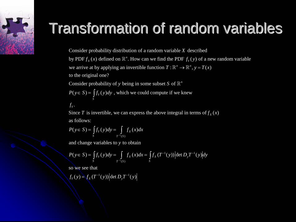
Transformation of random variablesTransformation of random variablesConsider probability distribution of a random variable describedby PDF ( ) defined on . How can we find the PDF ( ) of a new random variablewe arrive at by applying an invertible function :

nX Y

n

Xf x f y

T → , ( )to the original one?Consider probability of being in some subset of

( ) ( ) , which we could compute if we knew

.Since is invertible, we can express the above integral in t

n

n

YS

Y

y T x

y S

P y S f y dy

fT

=

∈ = ∫

1

1

( )

1 1

( )

1 1

erms of ( )as follows:

( ) ( ) ( )

and change variables to to obtain

( ) ( ) ( ) ( ( )) det ( )

so we see that

( ) ( ( )) det ( )

X

Y XS T S

Y X X yS ST S

Y X y

f x

P y S f y dy f x dx

y

P y S f y dy f x dx f T y D T y dy

f y f T y D T y

−

−

− −

− −

∈ = =

∈ = = =

=

∫ ∫

∫ ∫ ∫

Expected valueExpected value

For a random variable described by a probability densityfunction ( ), the expected value is

( ) ( )X

Xf x

E X x f x dx= ∫

(discrete gambling example)

“Prediction”

“Inference”

SingleStateVector

ProbabilityDensity functionon measurement

space

Measurement error and model stochasticity

(if present) introduce uncertainty

SingleMeasurement

vector

Probability densityFunction on state and

Parameter space

Measurement error, model stochasticity,

and ill-posedness introduce uncertainty

System states

Parameters

Quantitative

representation

of system

Measurement results

Mathematical model

of system

“Forward”

“Inverse”

“Int

erpr

etat

ion”

“Observation”

Sources of uncertainty in the forward and Sources of uncertainty in the forward and inverse problems, a more complete pictureinverse problems, a more complete picture

Bayesian inference for Bayesian inference for continouscontinous variablesvariables

|,|

||

( | ) ( )( , )( | )

( ) ( )while we also have

( ) ( , ) ( | ) ( )

so that( | ) ( )

( | )( | ) ( )

and can be vector valued, as well.So far, thi

Reca

s is

ll

that

j

Y X XX YX Y

Y Y

Y

Y X XX Y

f y x f xf x yf x y

f y f y

f y f x y dx f y x f x dx

f y x f xf x y

f y x f x dx

x y

= =

= =

=

∫ ∫

∫ust a statement about conditional

probability density functions (with the corresponding caveats...)The idea in Bayesian inference is now to use this in a setting where we obser data livi

ve song

me in y

|

and are interested in the distribution of parameters of some model living conditional on these observations. The conditional probability density fun space

in spacelike

ction( | ) is called li the Y Xf y x

x (and has been the object of our maximizing attempts so far.hood ..).

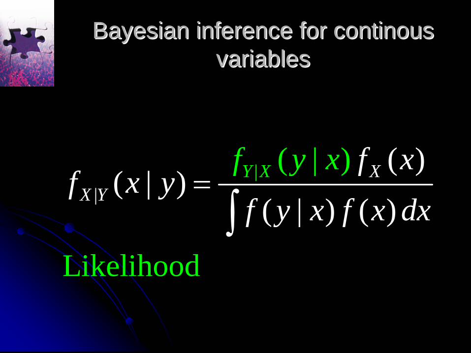
Bayesian inference for Bayesian inference for continouscontinous variablesvariables

||

( )( | )

( |( | )

Likelihoo

) ( )

d

XYX Y

X f xf x y

f y x f x dxf y x

=∫

ExampleExample

If the measurement errors for n measurements predictable by a model M are assumed to be independently and normally distributed, one could set up a likelihood function like this

2

2( ( ))

1

1( | ) ( )2

i i

i

y M xn

k i

f x y L x e σ

πσ

−−

=

= =∏

Bayesian inference for Bayesian inference for continouscontinous variablesvariables

||

( | ) ( )( | ) ( )

Probability density function

( | )

the posterior disof

tribution

YX Y

X Xff y x f xf y x d

yx

xf x

=∫

Bayesian inference for Bayesian inference for continouscontinous variablesvariables

||

( | )( | )

( | ) ( )

Probability density function of

( )

the prior distribution.

Y XX Y

Xf y xf x y

f y x f xf x

dx=∫

Bayesian inferenceBayesian inference

The underlying idea in Bayesian statistics is to identify probabilities with (subjective) degrees of belief in uncertain events. This conflicts with the more restrictive viewpoint of the frequentist philosophy, which accepts probabilities only as the relative frequency of occurrence of an event in a well defined random experiment. The extent to which this quantification of degree of belief is subjective is the matter of some debate.

Bayesian inferenceBayesian inference

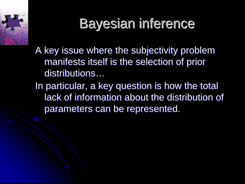
A key issue where the subjectivity problem A key issue where the subjectivity problem manifests itself is the selection of prior manifests itself is the selection of prior distributions…distributions…

In particular, a key question is how the total In particular, a key question is how the total lack of information about the distribution of lack of information about the distribution of parameters can be represented.parameters can be represented.

Prior distributionsPrior distributions

This question may seem innocent at first, but This question may seem innocent at first, but is in fact rather tricky and to my is in fact rather tricky and to my knowledge, no true consensus exists at knowledge, no true consensus exists at this point.this point.

Prior distributionsPrior distributionsIn the Bayesian spirit, priors can be used to implement the modelers belief (hopefully based on his domain expertise) about the distribution of parameters, e.g. along the lines of

•All values are equally probable (uniform distribution (on some interval), otherwise improper), or,

•The probability of each decade in the parameter range is equal (hyperbolic)

•Gaussian,

•etc.,etc.

Prior distributions and Prior distributions and reparametrizationreparametrization

It is crucial to recognize that the shape of a prior distributionand the specific parametrization of the model are linked:Consider for example a model ( ) of a single parameter . Let's assumethat o

y M x x=ur domain expertise leads us to believe that all values in

the interval [1,2] are equally likely, i.e., the prior is1 if 1 2

( )0 otherwise

Now consider a reparameterization of the model, e.g., by

X

xf x

≤ ≤⎧= ⎨⎩

1

11

ˆ

logarithmicallytransforming the independent variable:ˆ ˆ ˆ ˆ ˆ( ) ln , ( ) ( ) exp( )ˆ ˆ ˆ( ) : ( ( ))

ˆWhat does our prior distribution look like for ?

ˆ ˆ( )ˆ ˆ ˆ ˆ( ) ( ( )) (exp( ))expˆXX

x x x x x x x x

M x M x x

X

dx xf x f x x f xdx

−

−−

= = =

=

= =ˆ ˆexp( ) if 0 ln 2

ˆ( )0 otherwise

x xx

≤ ≤⎧= ⎨⎩

Prior distributions and Prior distributions and reparametrizationreparametrization

ˆ

Conversely, if we were to assume a uniform prior density on, e.g., [0, ln 2] for thelogarithmically transformed variable, the corresponding PDFfor the original variablewould be

1 if 11( ) (ln )X X

xf x f x x

x≤

= =2

0 otherwise

This kind of hyperbolic prior (uniform on the logarithmically transformedvariable) can be viewed as assigning equal probability to each decade of theparameter since

1( )ka

a

P a x ka dxx

⎧ ≤⎪⎨⎪⎩

≤ ≤ = ∫ ln ln lnka a k= − =

PriorsPriors

Invariance arguments can be brought into Invariance arguments can be brought into play to derive prior distributions that are play to derive prior distributions that are claimed to be as uninformative as claimed to be as uninformative as possible. The derivations are somewhat possible. The derivations are somewhat technical and we will not go into detail technical and we will not go into detail here. Well known examples include here. Well known examples include ““JeffreysJeffreys’ prior” for ’ prior” for parametrizedparametrized families of families of probability distributions and the soprobability distributions and the so--called called “reference priors”, each of which are not “reference priors”, each of which are not without issues (and may be expensive to without issues (and may be expensive to compute).compute).

Priors from a practical perspectivePriors from a practical perspectiveIf actual prior information is available, one should try to If actual prior information is available, one should try to incorporate itincorporate itOne needs to be aware of the interrelationship of model One needs to be aware of the interrelationship of model parametrizationparametrization and the shape of the prior distribution. If the and the shape of the prior distribution. If the phenomena modeled are well understood, a “canonical” phenomena modeled are well understood, a “canonical” parametrizationparametrization may be obvious on which the choice of a may be obvious on which the choice of a uniform prior, e.g., is physically meaningfuluniform prior, e.g., is physically meaningfulIf sufficient data is available, the effect of the prior may be If sufficient data is available, the effect of the prior may be smallsmallIf insufficient data is available, the prior will If insufficient data is available, the prior will dominatedominate, that , that is, the inference results will primarily depend on the choice is, the inference results will primarily depend on the choice of the priorof the priorExperimentation with different priors may (and should) Experimentation with different priors may (and should) reveal to what extent the conclusions drawn depend on the reveal to what extent the conclusions drawn depend on the choice of the priorchoice of the prior

Sampling to tackle high dimensional Sampling to tackle high dimensional problemsproblems

Full evaluation for analysis of functions of Full evaluation for analysis of functions of ofof the posterior density in high dimensions the posterior density in high dimensions intractable since it involves high intractable since it involves high dimensional integrals (e.g., 1D marginal dimensional integrals (e.g., 1D marginal will require computation of an (nwill require computation of an (n--1)1)--D D volume integral, expectation will require nvolume integral, expectation will require n--D volume integral, and so on and so D volume integral, and so on and so forth…)forth…)

Sampling to tackle high dimensional Sampling to tackle high dimensional problemsproblems

1

1

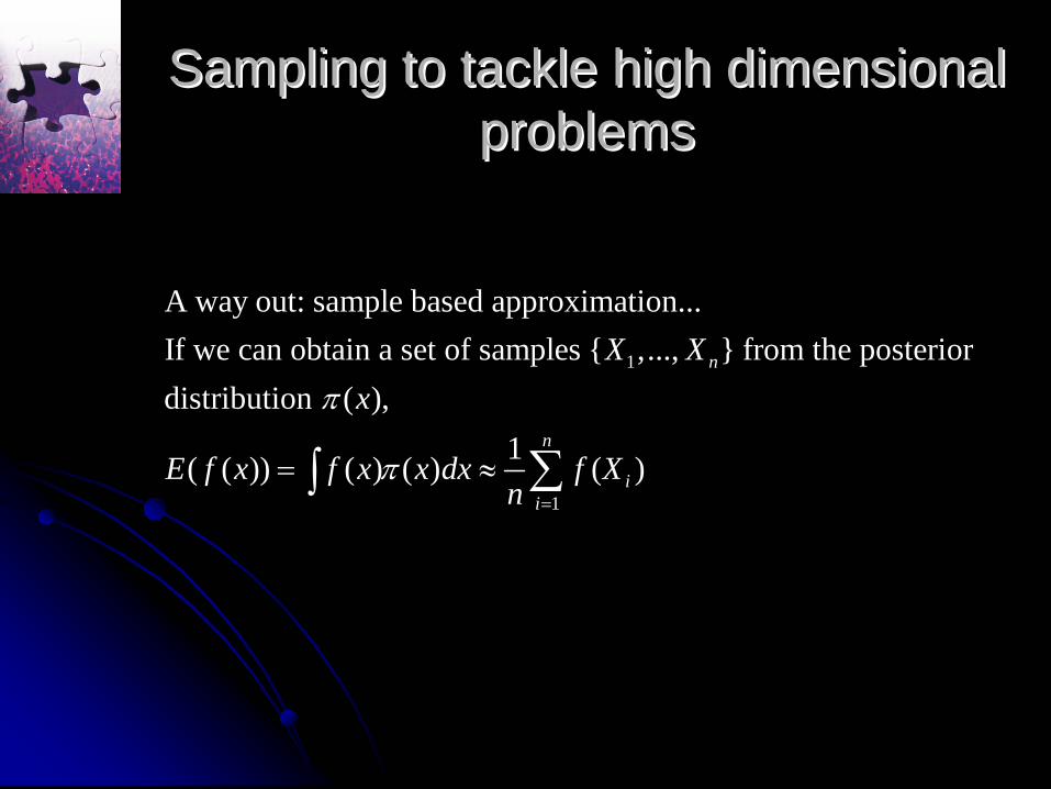
A way out: sample based approximation...If we can obtain a set of samples { ,..., } from the posteriordistribution ( ),

1( ( )) ( ) ( ) ( )

n

n

ii

X Xx

E f x f x x dx f Xn

π

π=

= ≈ ∑∫

What will therefore occupy us in the What will therefore occupy us in the futurefuture……

||

( | ) (( | )

( | ) ( ))Y X

XX

Yf xf

yf y x f x

f xx

y xd

=∫

How to sample from such a distribution given an implementation of the likelihood and the prior.

Assignment No. 8Assignment No. 8

1) Implement an (1) Implement an (unnormalizedunnormalized ) likelihood function corresponding to an ) likelihood function corresponding to an arbitrary number of independent observations with Gaussian arbitrary number of independent observations with Gaussian measurement noise for the unforced van measurement noise for the unforced van derder PolPol oscillator and plot the oscillator and plot the likelihood as a function of likelihood as a function of \\mumu on [0.05, 5] for the following scenarios, on [0.05, 5] for the following scenarios, using the parameters and initial conditions from homework no. 1 using the parameters and initial conditions from homework no. 1 unless unless stated otherwise. Describe your observations. Hint: it of coursestated otherwise. Describe your observations. Hint: it of course makes makes sense to implement a generic plotting routine that’ll handle allsense to implement a generic plotting routine that’ll handle all cases and cases and then run through the various combinations then run through the various combinations programaticallyprogramatically…)…)

a)a) 5, 10, and 20 measurements of both states simultaneously, with 5, 10, and 20 measurements of both states simultaneously, with measurements perturbed by additive Gaussian noise with standard measurements perturbed by additive Gaussian noise with standard deviations of 0.5, 1, and 2. Vary actual additive noise in the deviations of 0.5, 1, and 2. Vary actual additive noise in the measurements and the standard deviation you are using to computemeasurements and the standard deviation you are using to compute your your likelihood function independently a few times to observe their rlikelihood function independently a few times to observe their respective espective effects, but use the same values for both for the overall exploreffects, but use the same values for both for the overall exploration.ation.

b)b) Perform the same experiments as in a), but with observations forPerform the same experiments as in a), but with observations for only the only the 11stst and only the 2and only the 2ndnd state, respectively.state, respectively.

(for a total of 27 plots, as mentioned previously, you may wish (for a total of 27 plots, as mentioned previously, you may wish to automate to automate this)this)

2) Modify your plotting routine from 1) to plot the likelihood a2) Modify your plotting routine from 1) to plot the likelihood as a function of s a function of \\mumu \\in [0.05, 3] and the initial condition for state 1 in [0.05, 3] and the initial condition for state 1 \\in [0, 4], using the in [0, 4], using the surfcsurfc plotting function, and rerun the 9 scenarios where only state 2 plotting function, and rerun the 9 scenarios where only state 2 is is observed is observed. Describe your observations.observed is observed. Describe your observations.