Parallelization of the HIROMB Ocean Model7303/FULLTEXT01.pdf · Parallelization of the HIROMB Ocean...
120
Parallelization of the HIROMB Ocean Model Tomas Wilhelmsson Stockholm 2002 Licentiate Thesis Royal Institute of Technology Department of Numerical Analysis and Computer Science
Transcript of Parallelization of the HIROMB Ocean Model7303/FULLTEXT01.pdf · Parallelization of the HIROMB Ocean...

Parallelization of the HIROMB Ocean Model
Tomas Wilhelmsson
Stockholm 2002
Licentiate ThesisRoyal Institute of Technology
Department of Numerical Analysis and Computer Science

Akademisk avhandling som med tillstand av Kungl Tekniska Hogskolan framlag-ges till offentlig granskning for avlaggande av teknisk licentiatexamen mandagenden 10 juni 2002 kl 14.15 i sal D3, Kungl Tekniska Hogskolan, Lindstedtsvagen 5,Stockholm.
ISBN 91-7283-296-7TRITA-NA-0210ISSN 0348-2952ISRN KTH/NA/R--02/10--SE
c© Tomas Wilhelmsson, May 2002
Universitetsservice US AB, Stockholm 2002
Abstract
The HIROMB model of the North Sea and the Baltic Sea has been running oper-ationally at SMHI since 1995 and delivers daily forecasts of currents, temperature,salinity, water level, and ice conditions. We have parallelized and ported HIROMBfrom vector computers to distributed memory parallel computers like CRAY T3Eand SGI Origin 3800. The parallelization has allowed grid resolution to be refinedfrom 3 to 1 nautical miles over the Baltic Sea, without increasing the total runtime.
The grid decomposition strategy is designed by Jarmo Rantakokko. It is block-based and computed with a combination of structured and unstructured methods.Load balance is fine-tuned by assigning multiple block to each processor. We an-alyze decomposition quality for two variants of the algorithm and suggest someimprovements. Domain decomposition and block management routines are en-capsulated in F90 modules. With the use of F90 pointers, one block at a time ispresented to the original F77 code. We dedicate one processor for performing GRIBformatted file I/O which is fully overlapped with model time stepping.
Computation time in winter season is dominated by the model’s viscous-visco-plastic ice dynamics component. Its parallelization was complicated by the needfor a direct Gaussian elimination solver. Two parallel direct multi-frontal sparsematrix solvers have been integrated with parallel HIROMB: MUMPS and a solverwritten by Bruce Herndon. We have extended and adapted Herndon’s solver forHIROMB, and use ParMETIS for parallel load balancing of the matrix in each timestep. We compare the performance of the two solvers on T3E and Origin platforms.Herndon’s solver runs all solver stages in parallel which makes it the better choicefor our application.
ISBN 91-7283-296-7 • TRITA-NA-0210 • ISSN 0348-2952 • ISRN KTH/NA/R--02/10--SE
iii

iv

Acknowledgments
Many people have been involved in the parallelization of HIROMB and in themaking of this thesis. My advisors Prof Jesper Oppelstrup and Prof Bjorn Engquisthave supported me with great enthusiasm throughout my studies. Every chat withJesper has left me inspired and feeling a little bit wiser. Bjorn arranged for a verystimulating visit to his department at the University of California, Los Angeles(UCLA).
Dr Josef Schule initiated the work towards a parallel version of HIROMB andwe have collaborated on several conference papers and much of the work reportedin this thesis. Many thanks goes to him for his hospitality during my visits toBraunschweig. Dr Jarmo Rantakokko was also involved from the beginning andprovided the algorithms and program code for domain decomposition.
Dr Bruce Herndon, then at Stanford University, had great patience with mewhen explaining all the details about his linear solver in a long series of emails. The“Herndon solver” proved to be essential for the performance of parallel HIROMB.
Lennart Funkquist at SMHI and Dr Eckhard Kleine at BSH have helped outa lot with explaining the inner workings of HIROMB. Anette Jonsson at SMHIhas kept me continuously updated on the daily HIROMB operations and providedmany constructive comments to the thesis.
Anders Alund played important roles both at the very start and very end ofthis effort. First by declining an offer to parallelize HIROMB and thereby leav-ing the opportunity to me, and finally by insisting to get copies of this thesis forproofreading.
I started out at Nada in the SANS group working with software for computa-tional neuroscience. Dr Per Hammarlund, then a SANS graduate student, has beenmy most influential mentor as I entered the world of high performance computing.
Many thanks to my present and former colleagues at Nada and PDC with whomI had a great time both at and after work.
Finally, I would like to thank my family and friends for their never-endingsupport and strong confidence in me, even at times when my own confidence wasweak.
Financial support has been provided by the Ernst Johnson stipend fund, theParallel and Scientific Computing Institute (PSCI), KTH (internationaliserings-medel) and SMHI, and is gratefully acknowledged. Computer time was providedby the National Supercomputer Centre in Linkoping.
v

vi

Contents
1 Introduction 31.1 Baltic Sea forecasting at SMHI . . . . . . . . . . . . . . . . . . . . 31.2 Numerical ocean models . . . . . . . . . . . . . . . . . . . . . . . . 4
1.2.1 Ocean models compared to weather models . . . . . . . . . 81.3 High performance computer architecture . . . . . . . . . . . . . . . 81.4 Parallel program design . . . . . . . . . . . . . . . . . . . . . . . . 9
1.4.1 Parallel efficiency . . . . . . . . . . . . . . . . . . . . . . . . 101.5 Related work . . . . . . . . . . . . . . . . . . . . . . . . . . . . . . 12
1.5.1 Parallel ocean models . . . . . . . . . . . . . . . . . . . . . 121.5.2 Numerical methods . . . . . . . . . . . . . . . . . . . . . . . 141.5.3 Ice dynamics models . . . . . . . . . . . . . . . . . . . . . . 151.5.4 Parallelization aspects . . . . . . . . . . . . . . . . . . . . . 16
1.6 List of papers . . . . . . . . . . . . . . . . . . . . . . . . . . . . . . 171.7 Division of work . . . . . . . . . . . . . . . . . . . . . . . . . . . . 17
2 The HIROMB Model 192.1 Fundamental equations . . . . . . . . . . . . . . . . . . . . . . . . . 20
2.1.1 Momentum balance . . . . . . . . . . . . . . . . . . . . . . 212.1.2 Reynolds averaging . . . . . . . . . . . . . . . . . . . . . . . 222.1.3 Tracer transport . . . . . . . . . . . . . . . . . . . . . . . . 23
2.2 External forcing and boundary conditions . . . . . . . . . . . . . . 232.3 Numerical methods . . . . . . . . . . . . . . . . . . . . . . . . . . . 24
2.3.1 Barotropic and baroclinic modes . . . . . . . . . . . . . . . 252.3.2 Separating the vertical modes . . . . . . . . . . . . . . . . . 25
2.4 Grid configuration . . . . . . . . . . . . . . . . . . . . . . . . . . . 262.5 Numerical solution technique . . . . . . . . . . . . . . . . . . . . . 29
2.5.1 Space discretization . . . . . . . . . . . . . . . . . . . . . . 292.5.2 Time discretization . . . . . . . . . . . . . . . . . . . . . . . 302.5.3 Outline of the time loop . . . . . . . . . . . . . . . . . . . . 31
vii

viii Contents
3 Parallel Code Design 333.1 Serial code reorganization . . . . . . . . . . . . . . . . . . . . . . . 33
3.1.1 Multi-block memory management . . . . . . . . . . . . . . 343.1.2 Multiple grids . . . . . . . . . . . . . . . . . . . . . . . . . . 35
3.2 File input and output . . . . . . . . . . . . . . . . . . . . . . . . . 363.2.1 Parallelization of file I/O . . . . . . . . . . . . . . . . . . . 373.2.2 I/O optimizations . . . . . . . . . . . . . . . . . . . . . . . 39
4 Domain Decomposition 414.1 HIROMB domain decomposition methods . . . . . . . . . . . . . . 44
4.1.1 Multi-constraint partitioning . . . . . . . . . . . . . . . . . 444.1.2 Load balancing ice dynamics . . . . . . . . . . . . . . . . . 46
4.2 Finding a performance model . . . . . . . . . . . . . . . . . . . . . 464.3 Decomposition algorithm improvements . . . . . . . . . . . . . . . 504.4 Parameter sensitivity . . . . . . . . . . . . . . . . . . . . . . . . . . 534.5 Future work . . . . . . . . . . . . . . . . . . . . . . . . . . . . . . . 53
5 Ice Dynamics 555.1 Rheology . . . . . . . . . . . . . . . . . . . . . . . . . . . . . . . . 575.2 Numerical methods . . . . . . . . . . . . . . . . . . . . . . . . . . . 605.3 Evaluating solution quality . . . . . . . . . . . . . . . . . . . . . . 61
6 Parallel Direct Sparse Matrix Solvers 636.1 Matrix properties . . . . . . . . . . . . . . . . . . . . . . . . . . . . 63
6.1.1 Water level system . . . . . . . . . . . . . . . . . . . . . . . 636.1.2 Ice dynamics system . . . . . . . . . . . . . . . . . . . . . . 64
6.2 Available solver software . . . . . . . . . . . . . . . . . . . . . . . . 656.3 Direct sparse matrix solving . . . . . . . . . . . . . . . . . . . . . . 65
6.3.1 Multi-frontal factorization . . . . . . . . . . . . . . . . . . . 676.4 Interfacing the parallel solvers with HIROMB . . . . . . . . . . . . 68
6.4.1 Domain decomposition . . . . . . . . . . . . . . . . . . . . . 696.5 Solver performance on CRAY T3E-600 . . . . . . . . . . . . . . . . 70
6.5.1 Water level system . . . . . . . . . . . . . . . . . . . . . . . 706.5.2 Ice dynamics system . . . . . . . . . . . . . . . . . . . . . . 736.5.3 ParMETIS optimizations . . . . . . . . . . . . . . . . . . . 73
6.6 Solver performance on SGI Origin 3800 . . . . . . . . . . . . . . . 776.7 Other solvers . . . . . . . . . . . . . . . . . . . . . . . . . . . . . . 806.8 Conclusion . . . . . . . . . . . . . . . . . . . . . . . . . . . . . . . 81
7 Overall Parallel Performance 837.1 Parallel speedup . . . . . . . . . . . . . . . . . . . . . . . . . . . . 837.2 Analysis of a time step . . . . . . . . . . . . . . . . . . . . . . . . . 867.3 Conclusions and further work . . . . . . . . . . . . . . . . . . . . . 89

Contents ix
A Fundamental Equations 91A.1 Momentum balance and continuity . . . . . . . . . . . . . . . . . . 91A.2 Turbulence closure . . . . . . . . . . . . . . . . . . . . . . . . . . . 92
A.2.1 Horizontal momentum flux . . . . . . . . . . . . . . . . . . 92A.2.2 Vertical momentum flux . . . . . . . . . . . . . . . . . . . . 93A.2.3 Tracer mixing . . . . . . . . . . . . . . . . . . . . . . . . . . 94A.2.4 Non-local turbulence . . . . . . . . . . . . . . . . . . . . . . 95
A.3 Forcing and boundary conditions . . . . . . . . . . . . . . . . . . . 95A.3.1 Atmospheric forcing . . . . . . . . . . . . . . . . . . . . . . 95A.3.2 Open boundary forcing . . . . . . . . . . . . . . . . . . . . 97A.3.3 River runoff . . . . . . . . . . . . . . . . . . . . . . . . . . . 98A.3.4 Ocean wave forcing . . . . . . . . . . . . . . . . . . . . . . . 98
Bibliography 101

x

To my parents


Chapter 1
Introduction
The Swedish Meterological and Hydrological Institute (SMHI) makes daily forecastsof currents, temperature, salinity, water level, and ice conditions in the Baltic Sea.These forecasts are based on data from a High Resolution Operational Model ofthe Baltic Sea (HIROMB). Within the HIROMB project [27], the German FederalMaritime and Hydrographic Agency (BSH) and SMHI have developed an opera-tional ocean model, which covers the North Sea and the Baltic Sea region with ahorizontal resolution of 3 nautical miles (nm). This model has been parallelizedand ported from vector computers to distributed memory parallel computers. Itnow runs operationally on a CRAY T3E and an SGI Origin 3800. The added mem-ory and performance of the parallel computers have allowed the grid resolution tobe refined to 1 nm over the Baltic Sea, without increasing the total runtime. Thisthesis describes the efforts involved in parallelizing the HIROMB model.
1.1 Baltic Sea forecasting at SMHI
The use of numerical circulation models has a long tradition at SMHI. From themid 1970s, baroclinic 3D models have been used for analysis of environmental-oriented problems like spreading of oil, cooling water outlets from power plants andlong-term spreading of radio-active substances [24, 26, 100].
However, it was not until 1991 that the first use of an operational circulationmodel started at SMHI with a vertically integrated model covering the Baltic Seawith a resolution of 5 km and forced by daily weather forecasts and in- and outflowthrough the Danish Straits [25]. Later, in 1994 a barotropic 3D version of thePrinceton Ocean Model (POM) [14], covering both the North Sea and the BalticSea with 6 vertical levels and a horizontal resolution of 10 km, was set in operationaluse. With the POM model it was possible to give a more accurate forecast of surfacecurrents in all Swedish coastal water.
3

4 Chapter 1. Introduction
In 1995, a fruitful cooperation with the German BSH was started with the aimof a common operational system for the North Sea and Baltic Sea region. BSHhad already since 1993 a fully operational model working for the North Sea andBaltic Sea regions including an ice module and an interface to an operational wavemodel [60]. In transferring the BSH model to a more general Baltic Sea model, themain modifications of the model itself only composed of changing the nesting from aconfiguration adapted to the German waters to a more general one. The project gotthe acronym HIROMB with at the first stage Germany (BSH) and Sweden (SMHI)as participants. In 1999 the project group was extended with three additionalmembers: Denmark, Finland and Poland.
The first pre-operational HIROMB production started in summer of 1995 withdaily 24-hour forecasts running on a Convex 3840 vector-computer with a 3 nmgrid resolution. In 1997 the model was transferred to a CRAY C90 at the NationalSupercomputer Centre (NSC) in Linkoping, which made it possible to increase thedaily forecast length to 48 hours. During 1997–2000, the model code has succes-sively been parallelized [86, 107, 108, 109, 110] and a special method of partitioningthe computational domain has been developed [81, 82]. At present HIROMB runswith a 1 nm grid resolution on 33 processors of a SGI Origin 3800, with a CRAYT3E serving as backup.
Figure 1.1 illustrates the benefit of improved grid resolution by comparing 3 nmand 1 nm forecasts. In Figure 1.2 a time line of each processor’s activity during onefull time step is plotted using the VAMPIR tracing tool [73]. Such traces are usefulfor analyzing the behavior of a parallel program and the tracing data is furtherdiscussed in Section 7.2 on page 86.
1.2 Numerical ocean models
The dynamics of a fluid is well described by the Navier-Stokes equations, a set ofpartial differential equations (PDEs). In order to find approximate solutions to aPDE with a computer, the equations are discretized, whereby the derivatives arereplaced with difference quotients. In the discretization process, space is dividedinto a grid and time into steps. The difference formulae stemming from spatialderivatives can be represented with a stencil. The stencil shows which neighboringpoints in the grid that are used in the formulae for a given grid point. Higher ordermethods have larger stencils. In HIROMB a nine-point stencil is used when solvingfor sea surface height (SSH), see Figure 1.3.
Like most other ocean models, HIROMB uses spherical coordinates in the hor-izontal. For computing sea surface height, a 2D vertically averaged model is suf-ficient, but to represent stratification and depth varying currents a 3D represen-tation is necessary. Compared to the horizontal extents, the ocean is shallow andthe choice of vertical coordinate system and number of vertical layers is more orless independent from the horizontal resolution. In HIROMB fixed vertical levels(z-coordinates) are used.

1.2. Numerical ocean models 5
3 nm grid
1 nm grid
Figure 1.1. The benefit of increased resolution is illustrated with the same 48-hourforecast from September 26, 2000 with the old 3 nm grid above and the new 1 nmgrid below. The plots show a magnified portion of the Mid Baltic Sea and FinnishBay with arrows indicating surface current and colors salinity. Blue colors indicatelow salinity water from the Finnish Bay flowing into and mixing with the saltierBaltic Sea proper. In the 1 nm plot a current arrow is drawn for every ninth gridpoint to facilitate comparison.

6Chapter
1.Introduction
Continuity and momentum eqns(6 substeps) (T & S)
ParMETIS Factorize & solve(4 iterations)
Bulid Symbolicmatrix factorize
3nmgrid
12nmgrid
Ice dynamics1nm grid
Barotropic and baroclinic parts
Advection
Figure 1.2. VAMPIR time line plot of one full time step of a 1 nm forecast from May 5, 2000 on 17 processors of a CrayT3E-600. Time runs along the horizontal axis and processors along the vertical. The colors indicate different phases of thecomputation. Red is inactive time when waiting for messages from other processors, i.e. the master processor at the bottom.The many thin black lines represent messages sent between processors. (This figure is discussed in Section 7.2 on page 86.)

1.2. Numerical ocean models 7
Figure 1.3. When solving for sea surface height in HIROMB a nine-point stencilis used. The center grid point and its eight closest neighbors in a 3 × 3 block areused in the difference formulae.
The numerical schemes for solving time-dependent PDEs fall generally into twoclasses: explicit or implicit. In explicit methods the values for the next time stepn+ 1 are expressed directly in terms of values from the previous steps n, n− 1 etc.Explicit methods are straightforward to parallelize, but their time step is restrictedby the Courant-Friedrichs-Levy (CFL) stability constraint, ∆t < ∆x/c, where ∆t isthe time step, ∆x the grid spacing and c the wave speed in the model. Gravitationalsurface waves in the Baltic Sea move at around 50 m/s, which for a 1 nm grid wouldrestrict an explicit time step to 30 seconds.
Implicit methods, in which the new values at step n+ 1 are indirectly expressedin other unknown values at n + 1, are not restricted by a CFL criterion. But theyrequire the solution of a linear equation system at every time step and tend to bemore complex to parallelize. HIROMB makes use of a combination of explicit andimplicit methods with a base time step of 10 minutes, as is further described inChapter 2.
The grid spacing puts a limit on how fine structures that a model is able toresolve. By refining the grid, forecast resolution can be improved, but at the expenseof increased computer time and memory use. With explicit methods the time stephas to be reduced with finer grid spacing in order to maintain stability of themethod. Also the time step for implicit methods may have to be reduced forreasons of accuracy. A doubling of horizontal resolution will require an eight-foldincrease in computational work (four from the added number of grid points, andtwo from the smaller time steps).
A characteristic length scale for the dynamics of a rotating stratified system isthe internal Rossby radius, which for the Baltic Sea is on the order of 3 nm. In orderto fully resolve that scale, an order of magnitude finer grid of about 0.3 nm wouldbe desirable. Such a fine resolution is at the moment unattainable for operationalBaltic Sea forecasting, but with the parallelization of HIROMB a significant stephas been made with the refinement from 3 nm to 1 nm.
8 Chapter 1. Introduction
The Computational Science Education Project has a nice introduction to oceanmodeling which is available online [70]. In addition to the ocean fluid dynamicsmodel, HIROMB also contains a mechanical model for representing sea ice dynam-ics. It is highly nonlinear and based on Hibler’s standard ice rheology [51]. TheHIROMB ice model is further described in Chapter 5.
1.2.1 Ocean models compared to weather models
Meteorologists have been using the fastest computers available for doing numericalweather forecasting since the 1950s. Today the computationally most expensivepart in weather forecasting is not running the forecast model itself, but instead theanalysis phase, where the initial state of the atmosphere is estimated by combin-ing input from previous forecasts, satellite imagery, radio sondes etc. The field ofnumerical ocean forecasting is younger and less data is available for estimating ini-tial conditions. The current HIROMB forecast model has no analysis phase at all,which is possible for the shallow Baltic Sea as its dynamics is so strongly coupled tothe atmospheric forcing. Analysis of sea surface temperature (SST) from satelliteand ship data is however planned for the future.
As in the atmosphere, the ocean circulation contains a rich field of turbulenteddies. However, in contrast to the weather systems, with typical scales of the orderof a few 1000 km, the dimensions of the ocean vortices that correspond to the highsand lows of the atmosphere are only of the order of 50 km because of the weakerstratification of the ocean as compared to the atmosphere. Coupled atmosphere-ocean models for climate studies have been using a 9:2 ratio of atmosphere to oceangrid resolution [88].
Another difference between ocean models and atmospheric models is the shapeof the computational domain. Regional weather models use a grid with rectangularhorizontal extents and the same number of vertical levels everywhere in the domain.Ocean grids on the other hand have an irregular boundary due to the coastlines,sometimes also with holes in them from islands in the domain. This affects theconvergence properties of iterative solvers used for implicitly stepping the barotropicmode in ocean models and also makes the domain decomposition for parallelizationmore complex, see Chapter 4.
1.3 High performance computer architecture
Many consider the CRAY-1, introduced in 1976, to be the world’s first supercom-puter. The weather forecasting community has always been using the fastest com-puters available and in 1977 the first CRAY-1 machine on European ground wasinstalled by the European Center for Medium-Range Weather Forecasts (ECMWF)in Reading. In order to make efficient use of the machine’s vector processors, pro-grams had to be adapted or vectorized. In 1982, CRAY introduced the CRAY X-MP

1.4. Parallel program design 9
model which used the combined speed of four processors to achieve almost one bil-lion computations per second. In order to use the processors in parallel for solving asingle problem applications had to be adapted or parallelized. The four processorsof the X-MP shared the same memory which simplified their cooperation. Par-allelization involved inserting directives into the source code telling the compilerhow the work should be divided. Over time CRAY compilers reached the pointthat they could automatically parallelize programs without needing much guidancefrom the programmer.
CRAY’s parallel vector processor (PVP) line of machines evolved into the C90model in 1991 with up to 16 processors, the machine on which SMHI in 1997 wasrunning both HIROMB and the weather forecast model HIRLAM. By that timethe vector supercomputers where being replaced by massively parallel processing(MPP) machines built from commodity microprocessors. Each processor has itsown memory and they communicate by exchanging messages over a fast networkinterconnect. By distributing the memory, MPPs may scale up to hundreds ofprocessors, compared to tens of processors for shared memory machines like thePVPs. But distributed memory requires a more radical code restructuring andinsertion of message passing calls in order to get a parallel code. SMHI parallelizedtheir weather forecast system HIRLAM and moved it onto a CRAY T3E-600 with216 processors in late 1998. Preproduction runs of the parallelized HIROMB model,the topic of this thesis, started on the T3E in 1999.
In recent years a new type of machine has appeared. They try to combine thesimple programming model of shared memory processors (SMPs) with the scala-bility to many processors possible with distributed memory. The SGI Origin serieshas a cache coherent non-uniform memory access (cc-NUMA) architecture whichprovides a logically shared memory view of a physically distributed memory. Thisallows parallelization without explicit message passing calls, but the programmerstill has to be aware of where data is placed in memory in order to reach goodparallel speedup. Parallel codes based on message passing may run without changeon these machines. In late 2000 an SGI Origin 3800 was installed at NSC withabout three times better performance per processor than the T3E-600. HIRLAMand HIROMB could quickly be ported to the Origin, and both codes were runningoperationally in early 2001.
A current trend is heterogeneous machines, for example recent IBM SP systemwhere each node in the network is an SMP. For optimal performance, programsshould take advantage of the shared memory processing available in each node aswell as doing message passing between the nodes.
1.4 Parallel program design
The goal of parallelization is to split a computational task over several processors, sothat it runs faster than with just one processor. Geophysical models have predom-inately been divided along only the horizontal dimensions, so that each processor

10 Chapter 1. Introduction
Figure 1.4. By adding a layer of ghost points around each of the four processorregions (left), data from neighboring processors can be copied in (right) and stencilcomputations may be performed in the whole domain of each processor.
is responsible for a geographical region of the grid. Horizontal decomposition isenough to get a sufficient number of partitions and it also keeps the model’s ver-tical interactions unaffected by the parallelization. The processors cooperate byexchanging information when necessary. One example is when doing the horizontalstencil computations, where they will need values from the regions of neighboringprocessors in order to update the values along their borders. On an SMP, pro-cessors can directly read from regions assigned to other processors, but they haveto ensure that the data is updated and valid. On distributed memory machinesthe requested data has to be sent as messages between processors. By introducinga layer of ghost points around each processor’s region, see Figure 1.4, the stencilcomputations on distributed memory machines can be efficiently implemented.1
1.4.1 Parallel efficiency
The efficiency of a parallel program is often measured in terms of its speedup.Speedup is defined as the time for a serial program divided by the time for a parallelversion of the same program. Ideally, a parallel program running on N processorswould yield a speedup of N times. But in practice speedup levels off with moreprocessors, and might even go down if too many processors are added.2 There aretwo main reasons why ideal speedup cannot be achieved: parallel overhead andload imbalance.
1Ghost points are also beneficial for SMPs in avoiding false sharing and other cache-relatedproblems.
2Some programs may display super-linear speedup, i.e. run more than N times faster withN times more processors. One reason for this is that as the data set is divided into smaller andsmaller parts, they fit better and better in the processor’s cache memories. After the point whenthe whole data set fits in cache memory, speedup falls off again.

1.4. Parallel program design 11
Parallel overhead
Parallel overhead is the extra work that has to be done in a parallel program butnot in the corresponding serial program. It includes interprocessor communicationfor synchronizing the processors’ work, updating ghost points, doing reduction op-erations like global sums, performing data transfers between local and global arraysetc. The communication network in a distributed memory computer can be char-acterized by its latency and bandwidth. Latency is the time required to transfer aminimal message and bandwidth is the asymptotic transfer rate for large messages.With these parameters, a linear model of the network’s performance is
t(s) = l +s
b, (1.1)
where t(s) is the transfer time for a message of size s on a network with latency land bandwidth b. On machines with high latency it is beneficial to group messagestogether and send fewer but larger messages. The routines for updating ghostpoints in HIROMB have been constructed with this in mind, see Section 3.1.1.
Sometimes interprocessor communication can be avoided by duplicating com-putations. This counts however also as parallel overhead since some work is thenredundant, but it may be quicker than letting one processor do the computationand then communicate the result.
Load imbalance
The maximum attainable speedup is limited by the processor with the largest work-load. For good speedup it is necessary that all work is divided evenly over theprocessors, in other words that the grid partitioning has to be load balanced. Loadimbalance L is defined as the maximum workload wi on a processor divided by theoptimal workload per processor. If the processors have the same performance, theoptimal workload is equal to the mean workload,
L =maxwi∑Ni=1 wi/N
. (1.2)
If the work distribution is constant in time, static load balancing may be suffi-cient. But if the work load varies, dynamic load balancing and/or multi-constraintpartitioning may be necessary. With dynamic load balancing the actual load ismeasured during the computation and if too much unbalance is detected, the gridpartitioning is adjusted accordingly. Computing a new decomposition and redis-tributing the dataset takes time and adds to the parallel overhead. Dynamic loadbalancing works best when the load varies slowly in time and redistributions areinfrequent. If the work load varies between different sections of a program, multi-constraint partitioning can help by creating a single partitioning which balances allsections at once, see Section 4.1.1.
Not all sections of a program may be possible to parallelize. Some components,like for instance file I/O, may be left as a serial section. A serial section corresponds

12 Chapter 1. Introduction
η
−coordinatesz
η
−coordinatesσ −coordinates
η
ρ
Figure 1.5. Common vertical discretizations for ocean models. z-coordinatesrepresent vertical distance from a resting ocean surface. σ-coordinates are terrainfollowing and ρ-coordinates follow surfaces of constant potential density. η is thedeviation from the resting surface. (Adapted from [70].)
to the worst case of load imbalance and can severely limit the maximum achievablespeedup as indicated by the famous Amdahl’s law. Let S(N) be the speedup withN processors. Then S(N) is limited by
S(N) =ts + tp
ts + tp/N≤ 1 +
tpts
(1.3)
where ts is the time of serial fraction of the code and tp is the time of parallelizablefraction on one processor. If, say, a program is parallelizable to 90%, the maximumattainable speedup is 10 times. To get scaling up to large numbers of processors aprogram has to be close to 100% parallelizable.
File I/O in HIROMB is done serially but it is overlapped with computation asdescribed in Section 3.2. HIROMB uses static load balancing for the water model,and dynamic load balancing for the ice model, see Chapters 4 and 6. The overallparallel performance and speedup of HIROMB is discussed in Chapter 7.
1.5 Related work
Griffies et. al. [37] has reviewed the recent developments in ocean modeling withspecific reference to climate studies. A diverse set of codes is in use today andduring the 1990s many of them have been adapted for parallel computation. Inthis section we give a survey of parallel ocean models.
1.5.1 Parallel ocean models
The choice of vertical coordinate system is said to be the single most importantaspect of an ocean model’s design. Figure 1.5 shows the three main alternatives forvertical discretization. In the following overview, we group the models accordingto their vertical coordinates. Note that within each group many models have acommon ancestry.

1.5. Related work 13
Geopotential (z-coordinate) models
Geopotential vertical discretization is a common choice for coastal and sea-shelfmodels where a good representation of the surface mixed layer is important. HI-ROMB uses z-coordinates with the thickness of the lowest grid cell varying ac-cording to the bottom topography (the partial cell approach). A model with nu-merics similar to HIROMB is the Hamburg Ocean Primitive Equation (HOPE)model [31, 112]. Other parallel z-coordinate ocean models include the GFLD Mod-ular Ocean Model [78]. Currently in its third major revision, MOM3 has its rootsin the original Bryan-Cox-Semtner model from the 1960s. Many models have beenbased on earlier versions of MOM, for example the Southampton-East Anglia (SEA)model [10, 105] and the OCCAM model [40] developed within the British OceanCirculation Climate Advanced Modeling programme. The Rossby Centre at SMHIhas augmented OCCAM with an ice component and created the RCO model forclimate studies of the Baltic Sea [68]. Bremerhaven Regional Ice Ocean Simulations(BRIOS) has developed a model which is based on the MOM2 code [29].
Another widespread z-coordinate model is the Parallel Ocean Program (POP)which is being used as a component in several coupled climate models, for examplethe Parallel Climate System (PCM) [103]. POP was originally developed for theCM-2 Connection Machine [96] and was later ported [54] and optimized [102] forCRAY T3D and SGI Origin. POP descends from the Parallel Ocean Climate Model(POCM) which ran on CRAY vector machines [89].
Terrain following (σ-coordinate) models
Terrain following vertical coordinates are a commonly used in atmospheric models.In ocean models they provide a smooth representation of the bottom topographyand give increased vertical resolution in shallow regions where bottom boundarylayer processes are most important. The Princeton Ocean Model (POM) [14] hasbeen used extensively for ocean engineering applications. It has been parallelizedfor distributed memory machines using the source translation tool TOPAZ [76] andOpenMP directives have been added to improve load balance on heterogeneoussystems [66].
A number of σ-coordinate models have also been developed by groups at Rut-gers and UCLA, e.g., SPEM which later evolved into SCRUM [98]. SCRUM hasbeen completely rewritten to create the Regional Ocean Model System (ROMS)which includes OpenMP directives for shared memory, and with message-passingfor distributed memory in development [91].
Isopycnic (ρ-coordinate) models
Isopycnic coordinates are based on the potential density ρ referenced to a givenpressure. Tracer transport in the ocean interior has a strong tendency to occuralong directions defined by the potential density, rather than across, which makesisopycnic models suitable for representing dynamics in this regime. Examples of

14 Chapter 1. Introduction
isopycnic models include MICOM of which there are versions running on data-parallel, message-passing, shared-memory and heterogeneous machines [12, 84].The parallel design of MICOM is inherited in the new hybrid coordinate modelHYCOM [13]. The parallelization of POSEIDON, another hybrid model, is re-ported by Konchady et. al. [62]. The isopycnic NRL layered ocean model (NLOM)has been made portable to all machine types including data parallel and hetero-geneous systems [101]. OPYC was an early isopycnic model [74] parallelized forCRAY T3D [75], but it is not longer supported.
1.5.2 Numerical methods
A fundamental technique in ocean modeling is to split the solution of the mo-mentum equations into a barotropic and a baroclinic part, see Section 2.3. Thebarotropic part carries the fast dynamics of gravitational surface waves, leavingthe much slower deviations from the vertical average to the baroclinic part. Thismode splitting makes it possible to use different numerical methods for barotropicand baroclinic dynamics, which substantially improves efficiency. In a split-explicitapproach, where both parts are advanced with explicit methods, the barotropicpart has to be stepped with a much smaller time step than the baroclinic part. Byinstead solving the barotropic part implicitly, a common time step may be used.Various combinations of explicit and implicit methods have been employed by theocean modeling community. MICOM is an example of a purely explicit model whileHOPE and OPYC are fully implicit. Many models handle their horizontal interac-tions explicitly and their vertical interactions implicitly, for example HYCOM andPOM. This makes their parallelization easier as a horizontal decomposition doesnot affect their vertical solver.
Most models employ an explicit leap-frog scheme for stepping the baroclinicpart. A filter is necessary to remove the time-splitting computational mode in-herent in the leap-frog scheme. MOM, MICOM/HYCOM and POSEIDON all usea Robert-Asselin time filter, while ROMS uses an Adams-Molton corrector, POPuses time averaging, and OCCAM uses Euler backwards for filtering.
For the barotropic part, MOM (and its derivatives SEA and OCCAM), MI-COM/HYCOM, POSEIDON and ROMS use an explicit free surface method. MOMhas also implemented an implicit free surface method, which is also in use by HI-ROMB, HOPE, NLOM, OPYC and POP. In the implicit free surface method aHelmholtz equation is to be solved at each time step. Solvers can be grouped into ei-ther iterative or direct. Iterative solvers are more common and better suited for par-allelization. They are in use by OPYC which employs a line-relaxation method [74]and POP which uses a conjugate gradient method with local approximate-inversepreconditioning [96]. The NLOM model [101] has an iterative Red-Black SORsolver for the baroclinic part and uses the Capacitance Matrix Technique (CMT)for the barotropic part. CMT is a fast direct method based on FFTs. HOPE offersthe choice of either an iterative SOR method or a direct method based on Gaussianelimination for the barotropic part [112].

1.5. Related work 15
In regard to numerical methods for the barotropic part, HIROMB has most incommon with direct method used by HOPE. Both models do Gaussian eliminationand they assemble and factorize the matrix outside of the time loop. At each timestep only a back substitution step is necessary. Direct solvers are otherwise rarelyused in ocean models. For HIROMB the direct solver is necessary anyhow for itsice dynamics model, so it was a natural choice also for the barotropic part.
Slower convergence for iterative solvers on fine grids and difficulties in imple-menting implicit solvers on parallel computers has renewed the interest in explicitmethods. With increased resolution, the number of iterations for an iterative solvertends to increase, while the time step ratio between the baroclinic and barotropicparts stays constant for a split-explicit approach. With increasing number of ver-tical levels and improved model physics, the barotropic part of a model has ceasedto dominate the total computation time like it once did. The inherent data local-ity of explicit methods has made it much easier for them to achieve high parallelefficiency.
The review by Griffies et. al. [37] includes a discussion of solver choices, andrecent improvements to explicit free methods for z-coordinate models are also givenby Griffies et. al. in [36].
1.5.3 Ice dynamics models
Although there is now a large number of parallel ocean models in use, the numberof codes which include a parallelized ice dynamics model is still limited. Meierand Faxen [69] give a list of parallel ocean models which are coupled with a fullythermodynamic-dynamic ice model.3 The ice models of HIROMB [61], BRIOS [99],HOPE [112], MOM2 [29], OPYC [74], PCM [103], POCM [115], and RCO [68], areall based on Hibler’s viscous-plastic (VP) rheology [51].
Most models have started to use EVP, an Elastic regularization of the VPmodel [46]. One example is PCM which initially solved the VP model with linerelaxation [103]. In the second version of PCM [104] the ice component is replacedwith the CICE model [48] which implements EVP dynamics with an improvedcomputation of the stress tensor [47]. The EVP model is explicitly solved whichmakes it particularly easy to parallelize. The V-VP formulation in HIROMB, onthe other hand, requires the use of a direct sparse matrix solver and dominates theruntime in the winter season. It also accounted for a large part of the parallelizationeffort, see Chapters 5 and 6. To this author’s knowledge, HIROMB and the Germanice models employed at AWI in Bremerhaven (BRIOS and MOM2) and at DKRZin Hamburg (HOPE) are the only parallel ice models in use today which computeice dynamics with implicit methods.
3They also mention a Norwegian version of MICOM which is coupled to a serial ice modelwith EVP dynamics.

16 Chapter 1. Introduction
1.5.4 Parallelization aspects
The irregular shaped ocean coastlines makes the issue of domain decomposition andload balance an important aspect of the parallel design. For a global ocean modelgrid approximately 65% of the grid points are active water points. For a BalticSea grid the figure is lower still, with 26% active points for the rectangular gridcontaining HIROMB’s 1 nm model area. Early parallel implementations of oceanmodels ignored this fact and used a regular horizontal grid partitioning where everyprocessor gets an equally sized grid block. In many cases some processors wouldend up with a piece of the grid without any water points at all. MICOM [83] andPOSEIDON [62] use regular decompositions with more blocks so that the numberof blocks with water approaches the number of processors.
Load balance
Equally sized partitions is however not enough to achieve a good load balance asthe amount of active water points can vary substantially between partitions. Theparallelization of POM described by Luong et. al. [66] uses blocks of different shapesto minimize the number of unused land points in the grid. They alleviate loadimbalances by assigning more shared memory processors to larger blocks. ParallelHIROMB raises the water points fraction further by splitting the grid into moreblocks than there are processors and optimizing load balance as they are assignedto processors, see Chapter 4. The two closely related models OCCAM [40] andSEA [105] assign just one block per processor, but give the block an irregularoutline. This makes it possible to load balance with a granularity of individual gridpoints.
The spatial distribution of computational work may differ between differentcomponents of an ocean model. For instance, the work in the barotropic componentscales roughly with the amount of water surface, whereas the baroclinic componentdepends on the water volume. This is particularly true if ice dynamics is includedin the model, as the extent of ice cover varies dramatically in both space and time.The computationally most expensive part of HIROMB’s ice model is the linearsystem solver which has been load balanced separately, as described in Chapter 6.Another approach is to implement the ice component as a fully separate model, likefor instance is done in PCM [104] where atmosphere, ocean and ice components areindividually parallelized models interacting through a flux coupling library.
Overlapping computation with communication and file I/O
In addition to load imbalance, the attainable speedup for a parallel implementationis limited by overhead from interprocessor communication and serial code sections.Parallel HIROMB uses a dedicated master processor which takes care of file I/O,letting the other processors continue with the forecast uninterrupted. The time forfile I/O is in effect hidden from total runtime. Similar arrangements are in use inother ocean models.

1.7. Division of work 17
With suitable data structures it is also possible to improve speedup by over-lapping ghost point updates and other interprocessor communication with compu-tational work. OCCAM [40] and MICOM [84] overlaps ghost point updates withcommunication, but this is unfortunately hard to implement for HIROMB in itscurrent formulation.
1.6 List of papers
The parallelization of HIROMB has been reported at various international confer-ences:
1. Tomas Wilhelmsson. Parallel ice dynamics in an operational Baltic Seamodel. In Developments in Teracomputing, Proceedings of the Ninth ECMWFWorkshop on High Performance Computing in Meteorology. World Scientific,Singapore, 2001. In press.
2. Tomas Wilhelmsson, Josef Schule, Jarmo Rantakokko, and Lennart Funkquist.Increasing resolution and forecast length with a parallel ocean model. In Pro-ceedings of the Second International Conference on EuroGOOS, Rome, Italy,10–13 March 1999. Elsevier, Amsterdam, 2001. In press.
3. Tomas Wilhelmsson and Josef Schule. Running an operational Baltic Seamodel on the T3E. In Proceedings of the Fifth European SGI/Cray MPPWorkshop, CINECA, Bologna, Italy, September 9–10 1999.URL: http://www.cineca.it/mpp-workshop/proceed.htm.
4. Josef Schule and Tomas Wilhelmsson. Parallelizing a high resolution opera-tional ocean model. In P. Sloot, M. Bubak, A. Hoekstra, and B. Hertzberger,editors, High-Performance Computing and Networking, number 1593 in Lec-ture Notes in Computer Science, pages 120–129, Heidelberg, 1999. Springer-Verlag.
5. Tomas Wilhelmsson and Josef Schule. Fortran memory management forparallelizing an operational ocean model. In Hermann Lederer and FriedrichHertweck, editors, Proceedings of the Fourth European SGI/Cray MPP Work-shop, number R/46 in IPP, pages 115–123, Garching, Germany, September10–11 1998. Max-Planck-Institut fur Plasmaphysik.
1.7 Division of work
The HIROMB forecast model was originally designed and written by Dr EckhardKleine at the Federal Maritime and Hydrographic Agency in Hamburg, Germany.Before the author entered the project, Dr Josef Schule at the Institute for Scientific

18 Chapter 1. Introduction
Computing in Braunschweig, Germany rewrote the memory layout of HIROMB touse direct storage in three dimensional arrays.
I designed and wrote the block management modules and the parallelized I/Oroutines, both described in Chapter 3. The adaptation of the serial HIROMB codeto the parallel environment was a shared effort together with Dr Schule. Dr Schulewrote the grid management module and the transfer of boundary values betweendifferent grid resolutions. I carried out most of the bug tracking and validation ofthe parallel version.
Dr Jarmo Rantakokko at the Department of Scientific Computing, UppsalaUniversity designed the algorithms and wrote the code for domain decompositionused in HIROMB. I integrated his decomposition library into HIROMB, made somemodifications to it and evaluated the decomposition quality, see Chapter 4.
The parallelization of ice dynamics with integration and adaptation of Herndon’ssolver, MUMPS and ParMETIS, was done by me as described in Chapters 5 and 6.
Lennart Funkquist, Mikael Andersson and Anette Jonsson at SMHI are respon-sible for the day to day HIROMB operations and wrote the scripts which integratesHIROMB with SMHI’s forecasting environment. They have all been involved invalidating the parallel version for operational use.

Chapter 2
The HIROMB Model
HIROMB is a model based on the ocean primitive equations. It is similar to a modeldescribed by Backhaus [8, 9] and uses fixed levels in the vertical, i.e. z-coordinates.The horizontal discretization is uniform with a spherical coordinate representationand a staggered Arakawa C-grid [6]. Central differences have generally been usedto approximate derivatives. For the time discretization, explicit two-level methodshave been used for horizontal turbulent flux of momentum and matter, advectionof momentum and matter while implicit methods have been used for the barotropicgravity wave terms in the momentum equations and continuity equation and thevertical exchange of momentum and matter. From both a numeric and dynamicpoint of view, the model may essentially be divided into three components, thebarotropic part, the baroclinic part, and ice dynamics.
Barotropic part
A semi-implicit scheme is used for the vertically integrated flow, resulting in asystem of linear equations (the Helmholtz equations) over the whole surface forwater level changes. This system is sparse and non-symmetric due to the Coriolisterms. It is factorized with a direct solver once at the start of the simulation andthen solved for a new right-hand side in each time step.
Baroclinic part
Water temperature and salinity are calculated for the whole sea including all depthlevels. Explicit two-level time stepping is used for horizontal diffusion and ad-vection. Vertical exchange of momentum, salinity, and temperature is computedimplicitly. The two tracers, temperature and salinity are both advected the sameway, and handled with the same subroutine.
19

20 Chapter 2. The HIROMB Model
Ice dynamics
Ice dynamics occurs on a very slow time scale. It includes ice formation and melting,and changes in ice thickness and compactness. The equations are highly nonlin-ear and are solved with Newton iterations using a sequence of linearizations. Anew equation system is factorized and solved in each iteration using a direct sparsesolver. Convergence is achieved after at most a dozen iterations. The linear equa-tion systems are typically small, containing only surface points in the eastern andnorthern part of the Baltic Sea. In the mid winter season however, the time spentin ice dynamics calculations may dominate the total computation time. The icedynamics model is discussed further in Chapter 5 on page 55.
Coupling to other models
The operational HIROMB code is loosely coupled via disk I/O to the atmosphericmodel HIRLAM [39]. Atmospheric pressure, velocity and direction of wind, hu-midity and temperature, all at sea level, together with cloud coverage are the maininput, while sea level, currents, salinity, temperature, and coverage, thickness anddirection of ice are output. HIROMB is run once daily and uses the latest fore-cast from HIRLAM as input. There are plans to couple the models more tightlytogether in the future.
A North Atlantic storm surge model and tabulated tidal levels give sea levelinformation at the open boundary in the Atlantic. A hydrologic model [35] providesriver inflow and surface wave forcing comes from the HYPAS [32] model.
2.1 Fundamental equations
HIROMB is based on the ocean primitive equations, which govern much of thelarge scale ocean circulation. As described by Bryan [15] the equations consist ofthe Navier-Stokes equations subject to the Boussinesq, hydrostatic and thin shellapproximations. Prognostic variables are the active tracers (potential) temperatureand salinity, the two horizontal velocity components and the height of the seasurface.
Boussinesq approximation
The Boussinesq approximation means that density variations are only taken intoaccount in the momentum equation where they give rise to buoyancy forces whenmultiplying the gravitational constant. This is justified since ocean density typicallydeparts no more than 2% from its mean value. Equivalently, the vertical scale forvariations in vertical velocity is much less than the vertical scale for variations indensity, and fluctuating density changes due to local pressure variations is negligible.The latter implies incompressibility of the continuity equation.
2.1. Fundamental equations 21
Hydrostatic approximation
An examination of the orders of magnitude of the terms in the momentum equationshows that to a high degree of approximation, the vertical momentum balance maybe approximated by
0 = g +1
∂p
∂z. (2.1)
Here, g = 9.81 m/s2 is acceleration due to gravity, density, p pressure and z thevertical coordinate. This is usually referred to as the hydrostatic approximationand implies that vertical pressure gradients are due only to density.
Thin shell approximation
Consistent with the above approximations, Bryan also made the thin shell approxi-mation since the depth of the ocean is much less than the Earth’s radius, which itselfis assumed to be constant (i.e. a sphere rather than an oblate spheroid). The thinshell approximation amounts to replacing the radial coordinate of a fluid parcel bythe mean radius of the Earth, unless the coordinate is differentiated. Correspond-ingly, the Coriolis component and viscous terms involving vertical velocity in thehorizontal equations are ignored on the basis of scale analysis. For a review andcritique of the approximations commonly made in ocean modeling, see Marshall et.al. [67].
2.1.1 Momentum balance
With the approximations outlined above and neglecting molecular mixing, the mo-mentum equations expressed in spherical coordinates are
Du
Dt− tanφ
Ruv +
1Ruw = fv − 1
1R cosφ
∂p
∂λ, (2.2)
Dv
Dt+
tanφR
uu +1Rvw = −fu− 1
1R
∂p
∂φ, (2.3)
0 = g +1
∂p
∂z, (2.4)
where the total derivative operator in spherical coordinates is given by
D
Dt=
∂
∂t+
u
R cosφ∂
∂λ+
v
R
∂
∂φ+ w
∂
∂z. (2.5)
The coordinate φ is latitude and λ is longitude. The vertical coordinate z is positiveupwards and zero at the surface of a resting ocean. u, v and w are the velocity
22 Chapter 2. The HIROMB Model
components, and R = 6371 km the radius of the idealized spherical Earth. TheCoriolis parameter is given by
f = 2ω sinφ, (2.6)
where ω = 7.292 · 10−5 s−1 is the rotation rate of the Earth. With the Boussinesqapproximation the continuity equation becomes
1R cosφ
(∂u
∂λ+∂(cosφ v)
∂φ
)+∂w
∂z= 0. (2.7)
The continuity equation is used to diagnose vertical velocity.
2.1.2 Reynolds averaging
The flow in the ocean is more or less turbulent, and cannot be fully resolved ina computation due to limitations in computer capacity. To include the effects ofturbulence in the equations above, it is convenient to regard them as applied toa type of mean flow and to treat the fluctuating component in the same manneras the viscous shear stress. Following the statistical approach by Reynolds, theinstantaneous values of the velocity components and pressure are separated into amean and a fluctuating quantity
u = u + u′, v = v + v′, w = w + w′, p = p + p′ (2.8)
where the mean of the fluctuating components is zero by definition and the meandenoted by a bar is defined as u = 1
T
∫ T0udt. The averaging period has to be greater
than the fluctuating time scale but is more or less artificial as there is hardly no suchseparation of scales to be found in nature. Averaging the momentum equations andignoring density fluctuations in the acceleration terms result in a set of equationsusually referred to as the Reynolds equations for the mean flow.
With the Reynolds stresses included and neglecting the bar for mean quantities,we get the following equations for momentum balance
Du
Dt− tanφ
Ruv +
1Ruw − tanφ
Ru′v′ +
1Ru′w′
+1
R cosφ
(∂
∂λ(u′u′) +
∂
∂φ(cosφu′v′) +
∂
∂z(R cosφu′w′)
)
= fv − 1
1R cosφ
∂p
∂λ,
(2.9)
Dv
Dt+
tanφR
uu +1Rvw +
tanφR
u′u′ +1Rv′w′
+1
R cosφ
(∂
∂λ(v′u′) +
∂
∂φ(cosφ v′v′) +
∂
∂z(R cosφ v′w′)
)
= −fu− 1
1R
∂p
∂φ.
(2.10)

2.2. External forcing and boundary conditions 23
The new terms are called the Reynolds stresses and represent the non-resolvedscales of motion, i.e. what we here regard as turbulence. However, as the new setof equations is not closed, the Reynolds stress terms has to be expressed in themean quantities. The normal approach to this closure problem is to make use ofthe analogy with molecular viscosity concepts as was first outlined by Stokes andBoussinesq. This means that the stress components are expressed as proportionalto an eddy viscosity times the strain-rate of the mean flow. The expressions for theReynolds stresses are given in Appendix A.2 on page 92.
2.1.3 Tracer transport
With the same approximations as for the momentum equations and after applyingReynolds averaging, we get the following equations for salinity and temperature
DT
Dt+
1R cosφ
(∂u′T ′
∂λ+∂(cosφv′T ′)
∂φ
)+∂w′T ′
∂z= 0, (2.11)
DS
Dt+
1R cosφ
(∂u′S′
∂λ+∂(cosφv′S′)
∂φ
)+∂w′S′
∂z= 0. (2.12)
Temperature and salinity are coupled to the momentum equations by the equa-tion of state. It relates density to temperature, salinity and pressure, and beingnonlinear it represents important aspects of the ocean’s thermodynamics.
= (S, T, p) (2.13)
In HIROMB, is computed with the UNESCO formula [30].
2.2 External forcing and boundary conditions
HIROMB uses input from both an atmospheric and a hydrological model as wellas from an ocean wave model. SMHI runs the atmospheric model HIRLAM [39]four times per day on a grid encompassing an area from Canada in the west toUral in the east, and from the pole in the north to the Sahara desert in the south,see Figure 2.1. HIRLAM provides HIROMB with sea level pressure, wind at 10 mheight, air temperature and specific humidity at 2 m above surface and total cloudi-ness. These parameters fully control the momentum and thermodynamic balancebetween the sea surface and the atmosphere. The data is interpolated before it isapplied, as HIRLAM is run with a much coarser grid than HIROMB.
A storm surge model for the North Atlantic and tabulated tidal levels give thesea level at the open boundary between the North Sea and the North Atlantic. In-flow data of salinity and temperature at the open boundary is provided by monthlyclimatological fields. A sponge layer along the boundary line which acts as a bufferbetween the inner model domain and a “climatological reservoir” outside. A hy-drological model [35] gives fresh water inflow at 73 major river outlets.

24 Chapter 2. The HIROMB Model
Figure 2.1. The area covered by HIRLAM atmospheric forecast model. HIRLAMis the main source of forcing to HIROMB.
The operational wave model HYPAS [32] provides energy, mean direction andpeak frequency of wind waves including swell which is important parameters forestimating wave induced surface mixing and mass flux at the surface (Stoke’s drift1).More details on forcing and boundary conditions are given in Appendix A.3 onpage 95.
2.3 Numerical methods
Numerical solutions are computed within HIROMB by dividing the ocean volumeinto a three dimensional grid, discretizing the equations within each grid cell, andsolving these equations by finite difference techniques. The solution method couldbe formulated in a straightforward manner, but the result would be a numericallyinefficient algorithm. Instead, Bryan [15] introduced a fundamental technique toocean modeling in which the ocean velocity is separated into its depth averagedpart and the deviation from the depth average. The next section, which is adaptedfrom the MOM manual [78], introduces the ideas behind this approach.
1Stoke’s drift: Consider a body of water as multiple small layers. As wind passes over thewater surface, it places a shear stress on the top layer. That layer then applies a slightly smallershear stress on the next layer down. In this way, a surface stress will result in a greater transportnear the surface than near the bottom.
2.3. Numerical methods 25
2.3.1 Barotropic and baroclinic modes
As discussed in Gill [30], the linearized primitive equations for a stratified fluid canbe partitioned into an infinite number of orthogonal eigenmodes, each with a dif-ferent vertical structure. Gill denotes the zeroth vertical eigenmode the barotropicmode, and the infinity of higher modes are called baroclinic modes. Because ofweak compressibility of the ocean, wave motions associated with the barotropicmode are weakly depth dependent, and so correspond to elevations of the sea sur-face. Consequently, the barotropic mode also goes by the name external mode.Barotropic or external waves constitute the fast dynamics of the ocean primitiveequations. Baroclinic waves are associated with undulations of internal densitysurfaces, which motivates the name internal mode. Baroclinic waves, along withadvection and planetary waves, constitute the slow dynamics of the ocean primitiveequations.
In Bryan’s original model, the fast barotropic waves were filtered out completelyby putting a rigid lid as boundary condition at the upper surface. The depth aver-aged mode of a rigid lid ocean model corresponds directly to the barotropic modeof the linearized rigid lid primitive equations. Additionally, the rigid lid model’sdepth dependent modes correspond to the baroclinic modes of the linearized rigidlid primitive equations. Also in free surface models like HIROMB, the baroclinicmodes are well approximated by the model’s depth dependent modes, since thebaroclinic modes is quite independent of the upper surface boundary condition. Incontrast, the model’s depth averaged mode cannot fully describe the free surfaceprimitive equation’s barotropic mode, as it is weakly depth dependent. Therefore,some of the true barotropic mode spills over into the model’s depth dependentmodes. It turns out that ensuing weak coupling between the fast and slow linearmodes can be quite important for free surface ocean models [45]. The coupling, inaddition to the nonlinear interactions associated with advection, topography etc.,can introduce pernicious linear instabilities whose form is dependent on details ofthe time stepping schemes.
Regardless of the above distinction between vertically averaged and barotropicmode for free surface models, it is common parlance in ocean modeling to referto the vertically integrated mode as the barotropic or external mode. The depthdependent modes are correspondingly called baroclinic modes.
2.3.2 Separating the vertical modes
Although there are several technical problems associated with the separation intovertically averaged and vertically dependent modes, it is essential when buildinglarge scale ocean models.
Without separation, the full momentum field will be subject to the Courant-Friedrichs-Levy (CFL) stability constraint of the external mode gravitational sur-face wave speed, which is roughly
√gH ≈ 75 m/s for the deepest part of the HI-
ROMB model region with H ≈ 600 m. With an 1 nm grid resolution, the time step

26 Chapter 2. The HIROMB Model
24 oW
12oW
0o 12oE 24
o E
50 oN
55 oN
60 oN
65 oN
70 oN
Figure 2.2. The 12, 3 and 1 nm grids for the HIROMB model encapsulated bythe 24 nm grid for the North-East Atlantic storm surge model.
for an explicit method would be limited to around 25 seconds. With splitting, thetime step limit for the internal modes, which are roughly 100 times slower thanthe external mode, would instead be 40 minutes. The benefits of mode separationincrease with improved vertical resolution as the added vertical levels are subjectonly to the baroclinic mode time step.
2.4 Grid configuration
There are two main factors which determine the model area. First, each memberstate of the HIROMB project has their own interest area and though the mainregion of interest is the Baltic Sea, countries like Sweden, Denmark and Germanyalso want to cover Kattegat, Skagerrak and the North Sea. Second, the model areahas an open boundary to the Atlantic and there is no ultimate choice of its location.Both physical and computational aspects have to be taken into consideration, andthis has led to the configuration presented in Figure 2.2 and Table 2.1. All gridsuse uniform spherical coordinates in the horizontal.
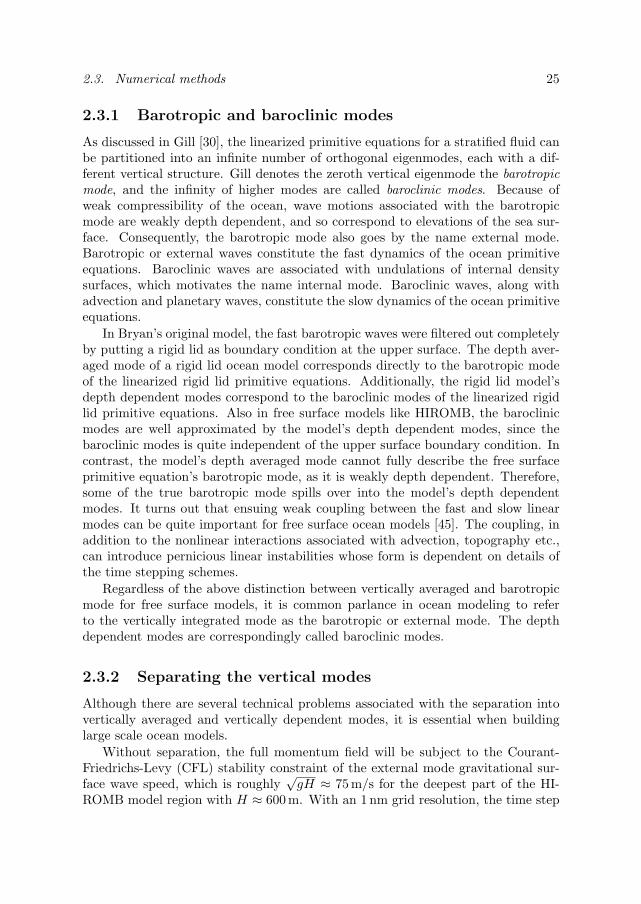
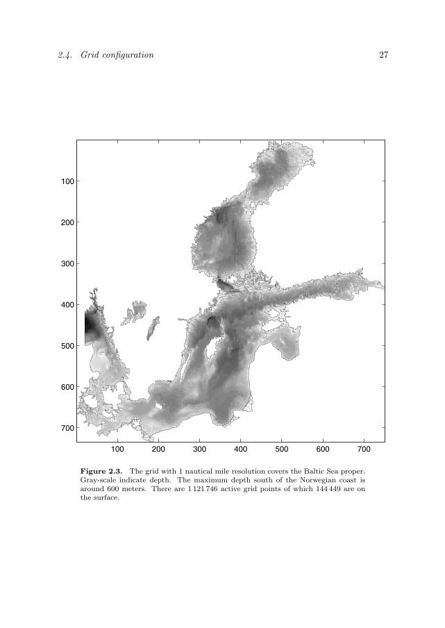
The 1 nm grid (see Figure 2.3) covers the Baltic Sea and Kattegat. Boundaryvalues at the open western border at 10 E are provided by a coarser 3 nm grid.This grid (see Figure 2.4) covers the waters east of 6 E and includes the Skagerrak,Kattegat, Belt Sea, and Baltic Sea. Boundary values for the 3 nm grid are providedby a coarser 12 nm grid (see Figure 2.4) which covers the whole North Sea and
2.4. Grid configuration 27
100 200 300 400 500 600 700
100
200
300
400
500
600
700
Figure 2.3. The grid with 1 nautical mile resolution covers the Baltic Sea proper.Gray-scale indicate depth. The maximum depth south of the Norwegian coast isaround 600 meters. There are 1 121 746 active grid points of which 144 449 are onthe surface.
28 Chapter 2. The HIROMB Model
50 100 150 200 250
50
100
150
200
250
20 40 60 80 100
10
20
30
40
50
60
70
80
Figure 2.4. The 3 nm grid, on top, provides boundary values for the 1 nm grid andhas 154 894 active grid points of which 19 073 are on the surface. The 12 nm grid,below, extends out to whole North Sea and has 9240 active grid points of which 2171are on the surface. It provides boundary values to the 3 nm grid. The sea level atthe open North Sea boundary of the 12 nm grid is provided by a storm surge model.

2.5. Numerical solution technique 29
Grid Points Points Longitude Latitudein W-E in N-S increment increment
HIROMB 1 nm 752 735 1’40” 1’HIROMB 3 nm 294 253 5’ 3’HIROMB 12 nm 105 88 20’ 12’Storm surge model 52 46 40’ 24’
Table 2.1. Horizontal configuration of the three HIROMB grids and the 24 nmNorth-East Atlantic storm surge model.
Baltic Sea region. All interaction between the grids takes place at the western edgeof the finer grid where values for flux, temperature, salinity, and ice properties areinterpolated and exchanged. In the vertical, there is a variable resolution startingat 4 m for the mixed layer and gradually increasing to 60 m for the deeper layers.The maximum number of layers is 24.
The 2-dimensional North-East Atlantic storm surge model which provides wa-ter level boundary values for the 12 nm HIROMB model runs with a 24 nm gridresolution. In the future, there are plans to extend the 1 nm grid to cover the samearea as today’s 3 nm grid and refine the 12 nm grid to 3 nm, as well as double thevertical resolution to a maximum of 48 layers.
2.5 Numerical solution technique
Much of HIROMB’s numerics stems from a model by Prof Jan Backhaus at Ham-burg University [8, 9]. HIROMB represents, however, a substantial update fromBackhaus’ model, for instance in areas like the water level equation, the implicittreatment of bottom stress as well as the advection scheme. The new physics hascalled for a more or less complete revision of the numerical methods, regarding boththe spatial and temporal discretization.
2.5.1 Space discretization
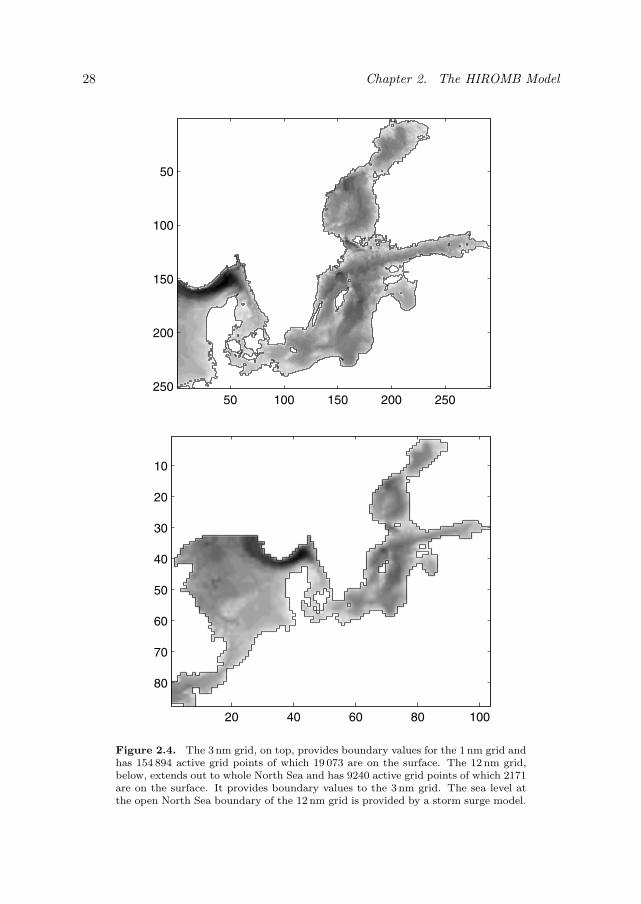
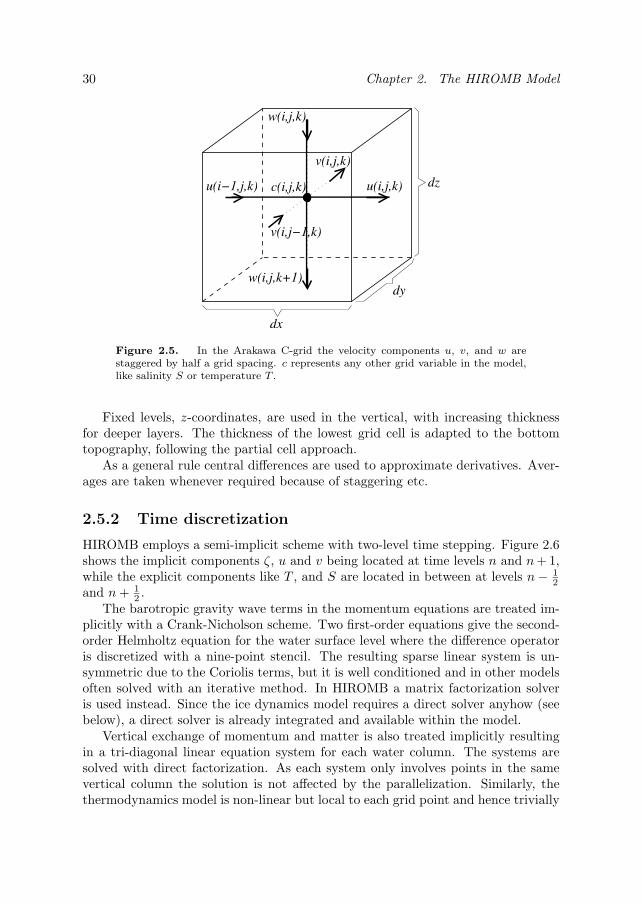
A number of options exists for how variables should be arranged in the grid. Themost widely used choice for high-resolution ocean modeling is the Arakawa C-grid [6]. It is a staggered grid in which the velocity components are offset by halfa grid spacing from the other grid variables, see Figure 2.5. The advantage ofthe C-grid lies in better dispersion properties and improvements in the geostrophicadjustment process as long as the horizontal resolution is less than the scale of theRossby radius. For the baroclinic part, the Rossby radius is typically of the orderof 4–8 km in the Baltic Sea compared to the present resolution of the model, whichis approximately 1.8 km.
30 Chapter 2. The HIROMB Model
dy
dx
v(i,j,k)
u(i,j,k)c(i,j,k)
w(i,j,k)
v(i,j−1,k)
w(i,j,k+1)
dzu(i−1,j,k)
Figure 2.5. In the Arakawa C-grid the velocity components u, v, and w arestaggered by half a grid spacing. c represents any other grid variable in the model,like salinity S or temperature T .
Fixed levels, z-coordinates, are used in the vertical, with increasing thicknessfor deeper layers. The thickness of the lowest grid cell is adapted to the bottomtopography, following the partial cell approach.
As a general rule central differences are used to approximate derivatives. Aver-ages are taken whenever required because of staggering etc.
2.5.2 Time discretization
HIROMB employs a semi-implicit scheme with two-level time stepping. Figure 2.6shows the implicit components ζ, u and v being located at time levels n and n+ 1,while the explicit components like T , and S are located in between at levels n− 1
2and n + 1
2 .The barotropic gravity wave terms in the momentum equations are treated im-
plicitly with a Crank-Nicholson scheme. Two first-order equations give the second-order Helmholtz equation for the water surface level where the difference operatoris discretized with a nine-point stencil. The resulting sparse linear system is un-symmetric due to the Coriolis terms, but it is well conditioned and in other modelsoften solved with an iterative method. In HIROMB a matrix factorization solveris used instead. Since the ice dynamics model requires a direct solver anyhow (seebelow), a direct solver is already integrated and available within the model.
Vertical exchange of momentum and matter is also treated implicitly resultingin a tri-diagonal linear equation system for each water column. The systems aresolved with direct factorization. As each system only involves points in the samevertical column the solution is not affected by the parallelization. Similarly, thethermodynamics model is non-linear but local to each grid point and hence trivially

2.5. Numerical solution technique 31
ζ , u, v ζ , u, vT, S T, S variables
time stepn+1n+1/2nn−1/2
Figure 2.6. Arrangement of time-levels for the implicit components (levels n andn + 1), and explicit system components (levels n − 1
2and n + 1
2), where the latter
concern baroclinic fields.
parallelized. The implicit treatment of the highly nonlinear ice dynamics model isfurther described in Chapters 5 and 6.
The remainder of the HIROMB model, like horizontal turbulent flux of momen-tum and matter, is solved explicitly. HIROMB’s advection scheme [59] is built onZalesak’s Flux Corrected Transport (FCT) scheme [113]. The FCT-scheme is ashock capturing algorithm which combines a conservative centered scheme with adissipative upwind scheme.
2.5.3 Outline of the time loop
The computations for one model time step are laid out as follows:
1. Update the interpolation of meteorological forcing fields.
2. Calculate density and baroclinic pressure from the hydrostatic equation.
3. Take into account the effects of surface waves.
4. Compute horizontal stresses and vertical eddy viscosity.
5. Solve equation of continuity and momentum equations (with sub-stepping):
(a) Set water level boundary values from a coarser grid or the external stormsurge model.
(b) Compute the RHS of the momentum equations.
(c) Insert the vertically integrated momentum (volume flux).
(d) Compute new water level by solving the Helmholtz equation.
(e) Solve the momentum equation with the new pressure.
6. Get boundary values for salinity and temperature from sponge layer.
7. Perform advection and diffusion of salinity and temperature.
8. Get boundary values for ice from sponge layer.

32 Chapter 2. The HIROMB Model
9. Dynamics of ice (ice momentum balance and constitutive equation):
(a) Set up matrix equation for the linearized ice dynamics model.
(b) Factorize and solve the matrix equation.
(c) Until convergence, update stress state projections and go back to step (b).
10. Advection of ice (thickness, compactness, and snow cover).
11. Heat flow at surface including ice thermodynamics (i.e. growth and melting).
The above stages are repeated for each grid. Currently, all grid resolutions usethe same 10-minute time step, giving 288 steps for a full 48-hour forecast. In thebarotropic solution (at stage 5), 2 sub-steps are taken for the 3 nm grid and 6sub-steps for the 1 nm grid.
Chapter 3
Parallel Code Design
As an initial effort it was decided to keep all algorithms and numerical methods inthe parallel version the same as in the serial version of HIROMB. This was possiblesince we had access to a direct sparse unsymmetric matrix solver for distributedmemory machines (Chapter 6). It was also desirable to maintain the file formatsof the serial version, so that auxiliary software like visualization packages wouldbe unaffected. This chapter describes how serial HIROMB was restructured forparallelization with special treatment of parallel file I/O in Section 3.2.
3.1 Serial code reorganization
The original serial version of HIROMB, which ran on a CRAY C90 vector com-puter, used an indirect addressing storage scheme to store and treat only the gridpoints containing water. While efficient in terms of memory use, this scheme wasexpected to have low computational efficiency on cache-based computers due toits irregular memory access pattern. Before this author entered the project, theindirect addressing storage was replaced with direct storage into regular two- andthree dimensional arrays. In this new scheme, a mask array is used to keep trackof if a grid point has water or land. The direct storage version of the code formedthe starting point for parallelization.
Our parallelization strategy is based on subdividing the computational gridinto a set of smaller rectangular grid blocks which are distributed onto the parallelprocessors. One processor may have one or more blocks. Software tools for handlinggrids divided into blocks in this manner are available, notably the KeLP packagefrom UCSD [22]. KeLP is a C++ class library providing run-time support forirregular decompositions of data organized into blocks. Unfortunately, we were notaware of this package when the HIROMB parallelization project started.
Serial HIROMB is almost entirely written in Fortran 77. The exception isa few low level I/O routines which use the C language. The new code added
33

34 Chapter 3. Parallel Code Design
for parallel HIROMB makes use of Fortran 90 features, but most of the originalcode is still Fortran 77. The Message Passing Interface (MPI) library is used forinterprocessor communication [97]. This makes parallel HIROMB portable to mostparallel computers available today. So far parallel HIROMB has been tested onCRAY T3E, SGI Origin, IBM SP, and a Compaq Alpha workstation cluster.
3.1.1 Multi-block memory management
The direct storage serial version represents each state variable in a two or threedimensional array covering the whole grid. In such an array only about 10% of thevalues are active water points. As discussed in Chapter 4, by decomposing the gridinto smaller subgrids, or blocks, many inactive land points can be avoided. Thefraction of active points in the subgrids, the block efficiency, increases with thenumber of subgrids. For parallel HIROMB we wanted to introduce several blocksper processor while still keeping as much as possible of the original code intact.This was done by replacing all arrays in the original code by Fortran 90 pointers.By reassigning these pointers, the current set of arrays is switched from one blockcontext to the next.
Within the computation routines the array indices still refer to the global grid.Unfortunately, Fortran 90 pointers do not support lower array bounds other thanthe default 1. Hence global grid indices cannot be used in the same routine aswhere block context is switched. However, this proved to be of no major concernsince block switching only has to take place in a few top level routines. Below is anexample of a basic code block in the parallel version of HIROMB:
! Do first part of ’flux’ routine!do b = 1, no blocks
if(.not. MyBlock(b)) cyclecall SetCurrentBlock(b)
call flux1(m1, m2, n1, n2, kmax, u, v, fxe, fye, ...)end do
call ExchangeBoundaries((/fxe id, fye id/))
Inside the flux1 routine, array dimensions are declared by their global indices withone line of ghost points added in each horizontal direction:
subroutine flux1(m1, m2, n1, n2, kmax, u, v, fxe, fye, ...)implicit none
integer m1, m2, n1, n2, kmax
real*8 u(m1-1:m2+1,n1-1:n2+1,kmax), v(m1-1:m2+1,n1-1:n2+1,kmax)
3.1. Serial code reorganization 35
real*8 fxe(m1-1:m2+1,n1-1:n2+1), fye(m1-1:m2+1,n1-1:n2+1)
integer i, j
do j = n1, n2do i = m1, m2
...
If ghost points need to be exchanged within one of HIROMB’s original routines,that routine is split into several parts. This has taken place in the example above,where the large routine flux in serial HIROMB was split into several routinesin parallel HIROMB with calls to ExchangeBoundaries in between. Note thatthe flux1 routine itself is not aware of more than one block at a time and maystill be compiled with a Fortran 77 compiler. All in all, there are 90 calls toSetCurrentBlock, and 39 calls to ExchangeBoundaries in parallel HIROMB.
Internally, the ExchangeBoundaries routine uses lists of block neighbors inorder to update the ghost points. If a neighbor block is located on the sameprocessor, boundary values are copied without calls to the communication library.For exchanges with blocks on other processors, buffered sends (MPI Bsend) followedby regular receives (MPI Recv) are used to avoid dead locks.
The block management routines, SetCurrentBlock, ExchangeBoundaries etc.are placed in Fortran 90 modules which encapsulate the low-level administrationcode for parallelization. The modules contain a list of all arrays that are decom-posed into blocks. New decomposed arrays may be added by changing just a fewlines of code. Each array has an associated handle, which is used in the call toExchangeBoundaries. Within the block management module all arrays with thesame number of dimensions n and type, e.g., three dimensional real, are storedtogether in an array with dimension n + 1. This reduces the number of MPI callsnecessary when exchanging boundaries between blocks without reverting to explicitpacking of messages. In the example above, the boundaries of both arrays fxe andfye are transferred in the same MPI call.1
File I/O is performed through a dedicated I/O processor. The block manage-ment module has routines for spreading out a global array from the I/O proces-sor to the workers (ScatterBlocks), and for assembling block data for output(GatherBlocks). These routines are called with the same array handle as used forExchangeBoundaries.
3.1.2 Multiple grids
Original HIROMB used two sets of arrays with different names, one for each gridin the model. In parallel HIROMB only one set of array names is used, and aroutine SetCurrentGrid is used to switch grid context in a manner analogous to the
1The MPI derived type mechanism could also have been used if an unique data type is createdfor each combination of arrays that appear in a call to ExchangeBoundaries.

36 Chapter 3. Parallel Code Design
Dataset Type Size Interval Total Format(Mbyte) (Mbyte)
Restart In/out 44.0 twice 88 Fortran, unformattedForcing In 0.3 3 hours 5 GRIBResults Out 12.6 1 hour 605 GRIB, bit-mapped
Table 3.1. The larger files which are read and written for the 1 nm grid during a48-hour forecast. Except for forcing, the same number of files are also accessed foreach of the coarser 3 nm and 12 nm grids.
way SetCurrentBlock switches block contexts. Data exchanges between grids arecurrently performed through one of the worker processors. The grid decompositionsare completely independent and do not regard geographical localizations. Theparallel version currently supports three different grids, and more grids may beadded with just minor code changes.
3.2 File input and output
Operational forecast models are often I/O intensive, and file input and outputcannot be neglected in a parallelization effort. Table 3.1 shows the larger filesinvolved in a 48-hour HIROMB forecast. A restart file is read at the beginning and anew one is written halfway through the forecast at 24 hours. Meteorological forcingfiles are read with an interval of three forecast hours and results are stored everyhour. The forcing and output files use the GRIB (gridded binary) standard [111],which is a very compact file format for representing meteorological data. The restartfile is stored as a regular unformatted Fortran file.
A GRIB file is grouped into description sections interleaved with data sections.Each data section stores a two-dimensional field. The compactness of GRIB isachieved by using only the necessary number of bits to store the values in the datasection. If, for example, a temperature is measured with one decimal precision andfalls in the range from -40 to +40, there are 800 possible values which may berepresented in 10 bits. Furthermore, for grids like HIROMB’s, with an irregularboundary, a bit-map may be used to store only the active points. This allows a rawdataset for the 1 nm grid2 of 291 Mbyte to be reduced to 12.6 Mbyte on disk.
Until mid 2000 bit-mapped GRIB had not been introduced in HIROMB andeach 1 nm result file was 59 Mbyte and stored every three hours. Including thecoarser grids, over 1 Gbyte of output was produced for a 48-hour forecast. Withthe recent introduction of bit-mapped GRIB storage, the output rate could beincreased to every hour adding up to 698 Mbyte per forecast. Although the amountof written data is reduced, the increased output rate invokes the output routine
2With a horizontal grid dimensions 752× 735, storing 4 3D-fields on 16 levels and 5 2D-fields,all in double precision (8 bytes per value).

3.2. File input and output 37
every sixth time step and could take a considerable fraction of the total time in aparallel implementation.
3.2.1 Parallelization of file I/O
Lockey et. al. has published a characterization of the I/O requirements in a mas-sively parallel sea shelf model running on a CRAY T3D [65]. Their I/O requirementsare similar to HIROMB’s with the same frequency of forcing input and result out-put and similar file sizes. As in HIROMB, the dominant I/O component is outputof results. They find that using a single processor for output creates a bottleneck,but that spreading the I/O operations over a few processors is enough for adequateperformance. Each processor then writes to a separate file and a post-processingstep is necessary to glue the files back together.
With the advent of the MPI-2 [72], there is now an machine independent stan-dard for doing parallel writes to a single file. Unfortunately, the interleaving of de-scription and data sections and the bit-oriented packing of the data section makes ithard to use parallel I/O routines in MPI-2 to read and write GRIB files. Hietanemiet. al. discuss the parallelization of GRIB I/O for the HIRLAM weather forecastmodel on an IBM SP system [44]. They also found it difficult to access a singleGRIB file in parallel and their solution was to write a pre- and post-processing toolwhich splits the input files into one for each processor before the forecast run, andthen pasting the output files together afterwards. These additional processing stepsare dependent on the number of processors and specific grid decomposition used inthe forecast run.
The approach taken in parallel HIROMB is instead to use a dedicated I/O pro-cessor. When writing, this allows the worker processors to carry on with theircomputation before the I/O operation is finished. Correspondingly, the I/O pro-cessor may complete a read operation before the data is required by the workers.As long as the I/O processor is quick enough to complete its task before the nextarrives, the I/O time may effectively be hidden completely from the model run-time. Similar dedicated I/O processor approaches has previously been used forboth atmospheric models [106] and ocean [40] models.
Input files
In serial HIROMB the initial model state was spread over three files, but for parallelHIROMB we have replaced them with a single restart file. Only the grid pointscontaining water are stored which limits the full 1 nm model state to 44 Mbyte. TheI/O processor reads the state variables one horizontal layer at a time and scattersthem to the workers. As this file is read and written only once per forecast, itsimpact on the total runtime is negligible.
The meteorological forcing for HIROMB is produced by the HIRLAM weatherforecasting model. In all 12 fields like wind speed, air temperature, humidity andcloud cover are provided in a GRIB formatted file. The weather model runs with

38 Chapter 3. Parallel Code Design
Figure 3.1. VAMPIR time line plots illustrating the overlap of GRIB outputand computation in a 3 nm forecast. In the upper graph the workers continue theircomputations uninterrupted, but in the lower graph they are stalled until the I/Oprocessor has finished its write operation. The upper graph shows 16 worker pro-cessors with a 17th I/O processor at the bottom. In the lower graph one of the16 worker processors is also responsible for I/O operations. Time runs along thehorizontal axis and processors along the vertical. Along the time dimension differentphases of the computation are shown in shades of gray. Note the repeating patternfrom time step to time step. The many thin black lines represent messages sentbetween processors. The diagonal lines show that all output messages are sent fromthe workers at the same time, but that the I/O processor receives them one by one.

3.2. File input and output 39
Architecture Compute Output Gather Reorder Pack Write(32 PEs) (sec) (sec) (sec) (sec) (sec) (sec)CRAY T3E-600 73 42 6 8 27 0.1SGI Origin 3800 27 9 3 1 5 0.1
Table 3.2. A comparison of the time to advance an 1 nm forecast 1 hour (six timesteps) to the time to output the result files. The last four columns show the outputtime split into gathering from workers to I/O processor, reorder and scaling, GRIBpacking and writing to disk. The write time is almost zero thanks to asynchronouswrite-behind buffering.
a coarser grid than the ocean model, and the forcing grid covering the largestHIROMB grid has dimensions 91 × 156. After reading the meteorological data isinterpolated to 12, 3, and 1 nm grid resolutions. The small size of the forcing gridmakes it possible to replicate it over all processors (with MPI Bcast) which theninterpolate those parts of the forcing grid that they require.
In addition to the files in Table 3.1 there are also a number of smaller filesproviding values for the open boundary in the North Atlantic and others specifyingfresh water inflow at 73 major river outlets. These files are also read by the I/Oprocessor and distributed to the workers.
Output files
HIROMB’s output for water consists of surface level, flow rate, temperature andsalinity, and for ice of thickness, compactness, and drift rate. Results are storedfor the upper 16 vertical levels of all HIROMB grids. With the use of bufferedsends (MPI Bsend) the workers are able to issue all their send operations and pro-ceed with their computations before the I/O processor has received all data. TheMPI Bsend calls return very quickly3 which allow the workers to proceed virtuallyuninterrupted, as is shown in Figure 3.1.
On T3E the raw amount of data for the 1 nm result file (291 Mbyte) would not fitin a single processor’s memory (128 or 256 Mbyte). Since a GRIB file is comprisedof a set of two-dimensional fields, only 4 Mbyte of data needs to be handled by theI/O processor at any one time. The rest of the data remains in the worker’s MPIbuffers until fetched by the I/O processor.
3.2.2 I/O optimizations
The strategy to overlap worker computation with I/O is dependent on the I/Oprocessor being able to keep up with the worker’s computational speed and outputrate. The time to output a GRIB file may be divided into time to fetch the data
3The amount of overlap possible between communication and computation may be dependenton the quality of the MPI implementation and the underlying hardware. We have so far verifiedthe overlap of computation and I/O on CRAY T3E and SGI Origin.
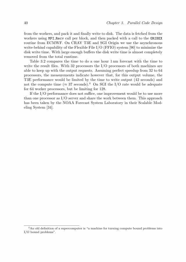
40 Chapter 3. Parallel Code Design
from the workers, and pack it and finally write to disk. The data is fetched from theworkers using MPI Recv call per block, and then packed with a call to the GRIBEXroutine from ECMWF. On CRAY T3E and SGI Origin we use the asynchronouswrite-behind capability of the Flexible File I/O (FFIO) system [90] to minimize thedisk write time. With large enough buffers the disk write time is almost completelyremoved from the total runtime.
Table 3.2 compares the time to do a one hour 1 nm forecast with the time towrite the result files. With 32 processors the I/O processors of both machines areable to keep up with the output requests. Assuming perfect speedup from 32 to 64processors, the measurements indicate however that, for this output volume, theT3E performance would be limited by the time to write output (42 seconds) andnot the compute time (≈ 37 seconds).4 On SGI the I/O rate would be adequatefor 64 worker processors, but be limiting for 128.
If the I/O performance does not suffice, one improvement would be to use morethan one processor as I/O server and share the work between them. This approachhas been taken by the NOAA Forecast System Laboratory in their Scalable Mod-eling System [34].
4An old definition of a supercomputer is “a machine for turning compute bound problems intoI/O bound problems”.

Chapter 4
Domain Decomposition
The computational grid for HIROMB, the Baltic Sea, has a very irregular shapewith varying depth. In order to make parallel HIROMB efficient, this workloadshould be evenly distributed over the processors, so that load balance is maximized,while at the same time inter-processor communication is minimized.
For irregular domains like the Baltic Sea, there are well established graph par-titioning algorithms like the Recursive Spectral Bisection (RSB) method [94]. Forlarge problems, multilevel methods quickly deliver high quality partitions. The stateof the art in multilevel algorithms is available in software packages like METIS [56]and Chaco [41]. All these methods generate partitionings where the boundarybetween two processor domains can take any shape.
Like most ocean models, the version of HIROMB used as starting point forparallelization employs block-based storage. Grid variables are stored directly inthree dimensional arrays with extents large enough to contain the whole computa-tional domain. The code loops over the full array dimensions and uses if-statementsfor avoiding unnecessary computations on land points. Unfortunately such an ar-rangement makes it cumbersome to directly use the irregular decompositions fromgraph partitioning algorithms. A decomposition method which splits the grid intoa set of smaller rectangular blocks lends itself better to the current structure of theHIROMB code.
In a rectangular block containing the whole 1 nm grid, only 26% of the surfacepoints and less than 10% of the volume points are active and contain water. Bydecomposing the grid into smaller rectangular blocks and discarding all blocks withno water points, it is possible to increase the block efficiency, i.e. the fraction of ac-tive points significantly. The blocks remaining are evenly distributed to the parallelprocessors. The grid is cut only along the north-south and east-west dimensionsand not between the surface and the sea bed. A further reduction in the number ofinactive grid points is achieved by allocating only the necessary number of verticallayers in each block, according to the maximum water depth in the block.
41

42 Chapter 4. Domain Decomposition
Figure 4.1. An illustration of the original domain decomposition method with the12 nm grid on 8 processors. (Upper left:) The domain is first divided into equallysized blocks. Blocks without any water are removed. (Upper right:) Blocks witha heavy work load are split further in order to get a more even workload. It iseasier to obtain a good load balance if the blocks have approximately the sameworkload. (Lower left:) Next, the blocks are shrunk before being distributed ontothe processors using a data distribution algorithm like recursive spectral bisection(RSB) or recursive coordinate bisection (RCB). (Lower right:) Blocks on the sameprocessor are combined and merged together in order to reduce the amount of blockboundary updating within each processor. As a final step, the number of inactivepoints is reduced further by shrinking the blocks where possible.

43
Figure 4.2. An illustration of the updated domain decomposition method with the12 nm grid on 8 processors. (Upper left:) The domain is split into halves and thetwo resulting blocks are shrunk to remove inactive points. (Upper right:) The firststep is repeated a number of times, where blocks with a lower than average fraction ofactive points are split and then shrunk. In this manner the block efficiency is kept upin the blocks. (Lower left:) The blocks are distributed onto the processors with therecursive spectral bisection (RSB) method. If the resulting load imbalance is abovea given threshold, one block is split to even out the load. (Lower right:) Therecursion continues until the number of partitions equals the number of processors.Blocks on the same processor are combined and merged together in order to reducethe amount of block boundary updating within each processor. As a final step, thenumber of inactive points is reduced further by shrinking the blocks where possible.

44 Chapter 4. Domain Decomposition
The geometry of the Baltic Sea forces the blocks to have different sizes andshapes in order to obtain a good load balance with minimal inter-block communi-cation. The more blocks the grid is decomposed into, the more inactive points canbe discarded. On the other hand, overhead from switching between blocks duringthe computation and updating block boundaries will increase with more blocks.Hence there is an optimal number of blocks which minimizes the total executiontime.
4.1 HIROMB domain decomposition methods
We use a domain decomposition package written by Dr Jarmo Rantakokko at Upp-sala University [80]. This package combines structured and unstructured methods.It consists of a set of low level operations that serve as building blocks for creating adiverse set of decomposition algorithms. The package was originally developed withthe HIROMB application in mind. We have used two main decomposition strate-gies with this package, the original algorithm as outlined in the 1998 paper [81] andan updated strategy described in [82], see Figures 4.1 and 4.2.
In the original algorithm, the domain is first split into a sufficiently large numberblocks, which are then distributed onto the processors. Timings have shown thatinactive (land) points amounts to a workload that cannot be ignored. Measurementsalso indicate that interprocessor communication time is fairly low on both Cray T3Eand SGI Origin systems. The updated strategy therefore puts more emphasis onload balance and block efficiency than communication volume (edge cuts). Here,the domain is first split up repeatedly with the blocks being shrunk to reduce theamount of land points in each iteration. The blocks are then distributed with arecusive bisection method. The new algorithm adds fine-tuning of the load balanceduring distribution by, if necessary, splitting a block between partitions at eachrecursion level. Figure 4.3 compares the output of the two algorithms. Note thatthe new algorithm gets a better load balance with a fewer number of blocks.
4.1.1 Multi-constraint partitioning
The workload of the three main components in HIROMB is not distributed equallyover the grid. The computationally most expensive component, ice dynamics, in-volves only those blocks with ice cover. The baroclinic workload depends on the to-tal number of active points in a block, i.e. the water volume, whereas the barotropicworkload also depends on the water surface area in the block. Note that for a do-main with varying depth, the ratio of water volume to water surface will differamong blocks.
Unfortunately it does not suffice to load balance the workload for all componentstogether. Interspersed in the code, in particular between the different components,there are interprocessor communication calls for updating block boundaries (seeSection 3.1.1). These calls synchronize the processors and expose any load balance

4.1. HIROMB domain decomposition methods 45
Figure 4.3. These decompositions of the 3 nm grid onto 16 differently shadedprocessors illustrate the difference between the two decomposition algorithms whenland point have zero weight. The old algorithm produced the 79 blocks on top withload balance 1.09. The new algorithm produced the decomposition below with 75blocks and load balance 1.01. Note that most of the blocks on top has been splitalong common lines, but that the new algorithm has split the blocks below morefreely. Furthermore the new algorithm has created a few narrow blocks which refinethe load balance, whereas the small blocks of the old algorithm is the result ofshrinking blocks with very few active points.

46 Chapter 4. Domain Decomposition
differences between them. A decomposition which balances only one constraint willnecessarily be a compromise if the load distribution varies between code sections.The METIS software package [56] can since version 4.0 do multi-constraint par-titioning and balance water surface, water volume and ice cover simultaneously,see Figure 4.4. Such a partitioning would potentially load balance all componentsof HIROMB. But as discussed above, the current version of HIROMB cannot useMETIS’ irregular partitionings. We instead use a performance model to find asingle constraint which best represents the accumulated workload of the barotropicand baroclinic components together, as is described in Section 4.2 below.
4.1.2 Load balancing ice dynamics
In order to maintain a decent load balance in winter, ice dynamics has to be treatedseparately. One strategy would be to use the algorithms described in Section 4.1above also for computing an ice cover partitioning. This has been evaluated forHIROMB by Schule [85]. At the start of each forecast run a new ice decompositionis computed. The ice covered area may grow during a 48-hour forecast run, but thiscan be accomodated by extending the ice decomposition to cover all water surfacewith a temperature sufficiently close to freezing. It was however decided not topursue this strategy in order to avoid the added code complexity from maintaingand updating two decompositions of the same grid. Furthermore, our experience isthat the block decomposition algorithms are not roboust enough to be integratedinto the daily forecast system. Occasionally, the generated decompositions may bebadly balanced and for 32 or more processors, decompositions with many blockssometimes fails to be computed at all.
Almost all ice dynamics time is spent in the sparse matrix solver. By usinga separate decomposition only for the matrix, the added complexity of anotherdecomposition may be contained within the solver itself and not affect the restof the HIROMB code. We partition the matrix with ParMETIS [57], a parallelversion of METIS, which includes a routine for sparse matrix partitioning, see Sec-tion 6.4.1. The efficiency of the parallel matrix factorization is highly dependent onthe amount of separator equations generated from the decomposition. ParMETISminimizes number of separator equations and can be expected to give better solverperformance than a block-based decomposition. ParMETIS is called once per timestep, and the extra time for computing the decomposition is offset by the muchreduced time for factorizing and solving a load balanced matrix.
4.2 Finding a performance model
In order to get a load balanced grid partitioning, the decomposition algorithmneeds a model of how the workload varies between blocks. A performance modelmay be developed from knowledge of the computational problem being solved andits performance on a particular machine. But for a complex code like HIROMB, it is

4.2. Finding a performance model 47
Water surface Water depth
Ice cover Partitioning on 16 processors
Figure 4.4. METIS can be used to generate a partitioning with an irregularboundary which balances water surface, water volume and ice cover at the sametime. In the 16 processor partitioning in the lower right, the amount of watersurface per processor is balanced to 2%, water volume to 1% and ice cover also to1%. The 1 nm grid used here has 144,449 vertices (water points) and 281,542 edges,of which 3304 were cut by processor boundaries. The partitioning was computed in2.5 seconds on one processor of an SGI-3800.
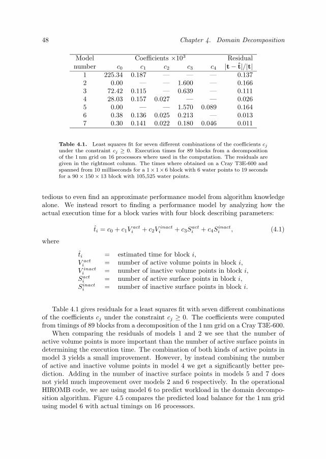
48 Chapter 4. Domain Decomposition
Model Coefficients ×103 Residualnumber c0 c1 c2 c3 c4 |t− t|/|t|
1 225.34 0.187 — — — 0.1372 0.00 — — 1.600 — 0.1663 72.42 0.115 — 0.639 — 0.1114 28.03 0.157 0.027 — — 0.0265 0.00 — — 1.570 0.089 0.1646 0.38 0.136 0.025 0.213 — 0.0137 0.30 0.141 0.022 0.180 0.046 0.011
Table 4.1. Least squares fit for seven different combinations of the coefficients cj
under the constraint cj ≥ 0. Execution times for 89 blocks from a decompositionof the 1 nm grid on 16 processors where used in the computation. The residuals aregiven in the rightmost column. The times where obtained on a Cray T3E-600 andspanned from 10 milliseconds for a 1× 1× 6 block with 6 water points to 19 secondsfor a 90× 150× 13 block with 105,525 water points.
tedious to even find an approximate performance model from algorithm knowledgealone. We instead resort to finding a performance model by analyzing how theactual execution time for a block varies with four block describing parameters:
ti = c0 + c1Vacti + c2V
inacti + c3S
acti + c4S
inacti , (4.1)
where
ti = estimated time for block i,V acti = number of active volume points in block i,V inacti = number of inactive volume points in block i,Sacti = number of active surface points in block i,Sinacti = number of inactive surface points in block i.
Table 4.1 gives residuals for a least squares fit with seven different combinationsof the coefficients cj under the constraint cj ≥ 0. The coefficients were computedfrom timings of 89 blocks from a decomposition of the 1 nm grid on a Cray T3E-600.
When comparing the residuals of models 1 and 2 we see that the number ofactive volume points is more important than the number of active surface points indetermining the execution time. The combination of both kinds of active points inmodel 3 yields a small improvement. However, by instead combining the numberof active and inactive volume points in model 4 we get a significantly better pre-diction. Adding in the number of inactive surface points in models 5 and 7 doesnot yield much improvement over models 2 and 6 respectively. In the operationalHIROMB code, we are using model 6 to predict workload in the domain decompo-sition algorithm. Figure 4.5 compares the predicted load balance for the 1 nm gridusing model 6 with actual timings on 16 processors.

4.2. Finding a performance model 49
0 2 4 6 8 10 12 14 160
0.2
0.4
0.6
0.8
1
Estimated load balance: 1.0672
Processor number
Est
imat
ed lo
ad
0 2 4 6 8 10 12 14 160
2
4
6
8
10
12
14
16
Measured load balance: 1.0841
Processor number
Ela
psed
tim
e pe
r st
ep
Figure 4.5. These bar graphs show the load balance for the 1 nm grid decomposedinto 60 blocks on 16 processors of an T3E-600. The top bar shows the estimatedload balance calculated by the decomposition algorithm, and the graph below showactual time per step (averaged over 18 steps).

50 Chapter 4. Domain Decomposition
Table 4.1 also shows the importance of minimizing the number of inactive gridpoints. Five land points are almost as computationally expensive as one waterpoint. We believe that this high cost for inactive points is due to wasted memorytraffic as whole cache lines are transfered even if there is only one active point inthem.
4.3 Decomposition algorithm improvements
We have introduced some minor improvements to the block splitting phase of theupdated decomposition algorithm [82], including:
• Split blocks with either low efficiency or high workload. If only blocks withlow efficiency are split, there might be blocks left with very large workload.Their workload may even be larger than the average workload per processor,making it impossible to achieve a load balanced decomposition.
• Do not split blocks if their absolute number of inactive points is too small. Ifonly the block efficiency is used as the split criterion, then there tend to be alarge number of tiny blocks along the coast lines.
• Do not combine blocks if their maximum depth differs too much. This keepsup the average block efficiency.
Both decomposition algorithms described in Section 4.1 assume that the totalworkload is independent of the decomposition. But a relatively high cost for inactivegrid points clearly invalidates this assumption. When the actual cost for inactivepoints is included in the performance model, the updated algorithm fails to achievemuch better load balance than the original strategy, as can be seen in Figure 4.6.
The distribution phase of the updated algorithm works recursively. All blocksare first divided into two groups, and if the load differs too much between the groups,one block is split to even out the load. We have improved this split operation sothat it makes an optimal split even in the presence of costly inactive points. But theload balance cannot be maintained through the recursion. At the next recursionlevel the original two groups are divided into four new groups, and if necessaryblocks are again split to achieve good load balance within each pair. However,since the dimensions of the newly split blocks usually can be shrunk a bit, the totalwork (including inactive points) for each new pair is reduced. This in turn destroysthe optimized load balance which was computed at previous recursion level. Thisexplains why the improved load balance of Figure 4.3 is not realized in practice inFigure 4.6.

4.3. Decomposition algorithm improvements 51
Figure 4.6. These decompositions of the 3 nm grid onto 16 differently shadedprocessors illustrate the difference between the two decomposition algorithms whena cost for inactive land point is included in the performance model. The originalalgorithm produced the 104 blocks on top with predicted load balance 1.20. Theupdated algorithm produced the decomposition below with 105 blocks and loadbalance 1.09. But the measured load balances are very similar with 1.12 for theoriginal and 1.11 for the updated algorithm.

52 Chapter 4. Domain Decomposition
0 100 200 3001.7
1.8
1.9
2
2.1
Number of blocks
Tim
e pe
r st
ep (
sec)
(a)
0 100 200 3000.4
0.5
0.6
0.7
Number of blocks
Ave
rage
blo
ck e
ffici
ency
(b)
1.05 1.1 1.15 1.2 1.25 1.31.7
1.8
1.9
2
2.1
Measured load balance
Tim
e pe
r st
ep (
sec)
(c)
0 100 200 3001.05
1.1
1.15
1.2
1.25
1.3
Number of blocks
Mea
sure
d lo
ad b
alan
ce
(d)
0.4 0.5 0.6 0.7 0.81.7
1.8
1.9
2
2.1
Average block efficiency
Tim
e pe
r st
ep (
sec)
(e)
0 100 200 3000.4
0.5
0.6
0.7
Number of blocks
Ave
rage
blo
ck e
ffici
ency
(f)
Figure 4.7. Scatter plots for 29 different decompositions of the 3 nm grid on 16processors, with time per step the best out of 18 steps. × indicates the original and the updated algorithm. (a) The best times are achieved with a little more than100 blocks. (b) For the same number of blocks, the updated algorithm gives slightlybetter block efficiency. (c) The best times are reached with balanced decompositions,and as can be expected (d) more blocks tends to improve load balance. (e) Shortertimes is surprisingly not correlated with higher block efficiency, but this is explainedin plot (f), which is the same as plot (b) but with symbol size indicating time perstep. High block efficiency is only achieved for decompositions with so many blocksthat other overheads take over.
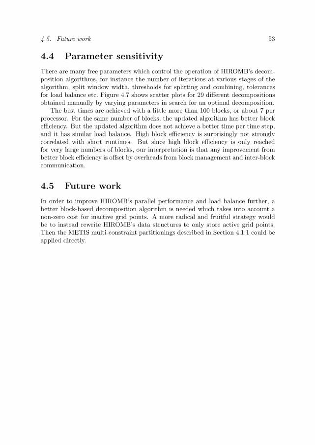
4.5. Future work 53
4.4 Parameter sensitivity
There are many free parameters which control the operation of HIROMB’s decom-position algorithms, for instance the number of iterations at various stages of thealgorithm, split window width, thresholds for splitting and combining, tolerancesfor load balance etc. Figure 4.7 shows scatter plots for 29 different decompositionsobtained manually by varying parameters in search for an optimal decomposition.
The best times are achieved with a little more than 100 blocks, or about 7 perprocessor. For the same number of blocks, the updated algorithm has better blockefficiency. But the updated algorithm does not achieve a better time per time step,and it has similar load balance. High block efficiency is surprisingly not stronglycorrelated with short runtimes. But since high block efficiency is only reachedfor very large numbers of blocks, our interpretation is that any improvement frombetter block efficiency is offset by overheads from block management and inter-blockcommunication.
4.5 Future work
In order to improve HIROMB’s parallel performance and load balance further, abetter block-based decomposition algorithm is needed which takes into account anon-zero cost for inactive grid points. A more radical and fruitful strategy wouldbe to instead rewrite HIROMB’s data structures to only store active grid points.Then the METIS multi-constraint partitionings described in Section 4.1.1 could beapplied directly.

54

Chapter 5
Ice Dynamics
The ice cover is regarded as a granular rubble of ice floes and modeled as a 2Dcontinuously deformable, and compressible medium. An ice model consists of twomain components: thermodynamics, i.e. growth and melting, and dynamics, i.e.drift. HIROMB’s ice thermodynamics is based on the Semtner zero-level model [87]and is described in [27]. Ice growth and melting, being a local process, is triviallyparallelized and will not be discussed further here.
The ice dynamics model computes forces and deformation. Thus, its compo-nents are an equation of motion (momentum budget) and a constitutive equationwhich gives the response of the ice to deformation. To close the system, there arealso evolution equations for the remaining budget quantities ice thickness hi, icecompactness A, and snow cover thickness hs.
The basic equations for momentum balance of sea ice come from 2D-continuummechanics, in the case of plane stress. In spherical coordinates, we have
ihi
(Du
Dt− tanφ
Ruv − fv + g
1R cosφ
∂ζ
∂λ
)= τλw + τλa + Fλ, (5.1)
ihi
(Dv
Dt− tanφ
Ruu + fu + g
1R
∂ζ
∂φ
)= τφw + τφa + Fφ. (5.2)
where tangential drag from water currents and wind is
τλw = cww√
(uw − u)2 + (vw − v)2(uw − u), (5.3)
τφw = cww√
(uw − u)2 + (vw − v)2(vw − v), (5.4)
τλa = caa√
(ua − u)2 + (va − v)2(ua − u), (5.5)
τφa = caa√
(ua − u)2 + (va − v)2(va − v). (5.6)
55

56 Chapter 5. Ice Dynamics
and forces due to internal stresses
Fλ =1
R cosφ
(∂σ11
∂λ+∂(cosφσ12)
∂φ
)− tanφ
Rσ12, (5.7)
Fφ =1
R cosφ
(∂σ21
∂λ+∂(cosφσ22)
∂φ
)+
tanφR
σ11. (5.8)
To characterize the deformation properties of the hypothesized large-scale con-tinuum mechanics material, use is made of Reiner-Rivlin equations as the generalform of constitutive equations of a fluid.1 The stress tensor components are
σ11 = ζ(ε11 + ε22) + η(ε11 − ε22) − P
2, (5.9)
σ12 = 2ηε12, (5.10)σ21 = 2ηε21, (5.11)
σ22 = ζ(ε22 + ε11) + η(ε22 − ε11) − P
2. (5.12)
where ζ and η are nonlinear bulk and shear viscosities, and P/2 is a reference pres-sure. The pressure is a measure of ice strength and depends on both ice thicknessand compactness. In spherical coordinates, the rates of deformation read
ε11 =1
R cosφ∂u
∂λ− tanφ
Rv, (5.13)
ε12 = ε21 =12
(1R
∂u
∂φ+
tanφR
u +1
R cosφ∂v
∂λ
), (5.14)
ε22 =1R
∂v
∂φ. (5.15)
It is assumed that large-scale pack ice is isotropic so that its mechanical behaviormay be stated in terms of invariants of stress and strain rate
σI =12
(σ11 + σ22), (5.16)
σII =12
√(σ11 − σ22)2 + 4σ12σ21, (5.17)
εI = ε11 + ε22, (5.18)
εII =√
(ε11 − ε22)2 + 4ε12ε21. (5.19)
Given these definitions, the constitutive equations, in terms of invariants, read
σI +P
2= ζεI , (5.20)
σII = ηεII . (5.21)
1Note that a fluid has no reference configuration. Thus, elastic phenomena are excluded.

5.1. Rheology 57
1σ / P
C
S
S
O
P2σ /
Figure 5.1. Hibler’s elliptical yield curve in principal stress space normalized withice pressure P . For plastic flow the stress states lie on the ellipse with the locationdictated by the ratio of the strain rate principal components. The stress state forpure shearing deformation is located at S and for isotropic compression at C. For verysmall strain rates, the stress states move inside the yield curve. (Adapted from [58].)
5.1 Rheology
A rheology relates stress to strain rate, and may be expressed through the nonlinearviscosities ζ, and η. Studies during the Arctic Ice Dynamics Joint Experiment(AIDJEX) in the 1970s [17] indicated that rate-independent plastic rheologies wereappropriate for modeling sea ice dynamics. With a rigid-plastic rheology, the icecover behaves like a solid resisting stress without deformation up to a yield limit,beyond which it flows with constant internal stress. It is common to let the yieldlimit take the shape of an ellipse in the space of principal stresses, see Figure 5.1.By locating the yield ellipse as in the figure, the ice cover is allowed to diverge withlittle or no stress, while strongly resisting compressive and shearing deformationunder convergent conditions.
To construct a numerical model, the AIDJEX project proposed an elastic-plasticrheology in which the deformation is proportional to the stress below the yieldlimit [18]. However, the introduction of elasticity entails keeping track of the strainstate of a given ice portion indefinitely, with substantial theoretical [79] and numer-ical [16] difficulties. In 1979 Hibler proposed a viscous-plastic (VP) rheology whichhas become the standard sea ice dynamics model [51, 52]. The essential idea is toapproximate the rigid or elastic portion of the plastic continuum by a state of very
58 Chapter 5. Ice Dynamics
slow creep. For small strain rates the ice behaves like a viscous2 fluid, whereas forlarge strain rates it flows in a plastic manner. A recent evaluation of different seaice rheology schemes may be found in [58].
Hibler specified the nonlinear viscosities as follows. Let
∆ =√ε2I + (εII/e)2 (5.22)
be one more invariant of the strain-rate tensor with e = 2. The viscosities increasewith pressure and with decreasing strain rate:
ζ =1
max(∆,∆0)P
2, (5.23)
η =1e2ζ. (5.24)
where ∆0 determines the switch between the viscous and plastic regimes. In Hibler’smodel ∆0 limits value of ζ to ζmax = 2.5 · 108P g/s. The pressure P , a measure ofice strength, is given by
P = P h e−c(1−A), c = 20, P = 27500 N/m2. (5.25)
where c and P are empirically determined parameters. The state of stress is thenconfined to the yield ellipse
(σI +P
2)2 + (eσII)2 =
(∆
max(∆,∆0)
)2(P
2
)2
≤(P
2
)2
, (5.26)
with e being the eccentricity of the ellipse.To avoid numerical instabilities Hibler also bounded the viscosities from below
with ζmin = 4 · 1011 g/s. In HIROMB another modification to the rheology is em-ployed. Kleine and Sklyar [61] found that it was appropriate to relax the plasticitycondition by admitting that the yield curve is exceeded. For sufficiently large ratesof strain, it should be possible to attain any stress. In practice, however, the stressstays in the neighborhood of the yield curve. Figure 5.2 shows schematically thestress as a function of strain rate.
Thus, the constitutive equation of HIROMB’s ice model is viscous-viscoplastic(V-VP) rather than viscous-plastic. Take some very small non-dimensional κ > 0parameter and let
ζ =1 + κmax( ∆
∆0− 1, 0)
max(∆, ∆0)P
2, (5.27)
η =1e2ζ. (5.28)
2It has been demonstrated that if time and/or length scales are chosen large enough, theaveraging of nonlinear (plastic) stochastic fluctuations in sea ice deformation rates yields a viscous-like law [50].

5.1. Rheology 59
Stress σ
Strain rate d /dtε
−P/2
Figure 5.2. One-dimensional view of the constitutive law in the Kleine and Sklyarviscous-viscoplastic modification to Hibler’s viscous-plastic model. The graph givesthe stress as a function of strain rate. Up to the yield limit, within the shadedregion, the viscosity is large, but beyond that the plastic viscosity is very small andcontrolled by the parameter κ.
Compared to equation (5.26), we now have
(σI +P
2)2 + (eσII)2 =
(∆∆0
∆0 + κmax(∆ − ∆0, 0)max(∆, ∆0)
)2(P
2
)2
. (5.29)
As shown in [61], introducing the parameter κ as a (minor) modification of Hibler’smodel amounts to regularizing the ice mechanics problem.
To close the ice dynamics model, there are two conservation equations for (mean)thickness and compactness:
∂h
∂t+
1R cosφ
(∂(uh)∂λ
+∂(cosφvh)
∂φ) = 0, (5.30)
∂A
∂t+
1R cosφ
(∂(uA)∂λ
+∂(cosφvA)
∂φ) = R(A). (5.31)
While the total mass of ice, given by its areal density h is conserved under transport,compactness in general is not. To prevent local compactness from exceeding unity,as could happen in cases of convergence, a sink term, the so-called ridging functionR ≤ 0, appears in the equation.3
3Keep in mind that there is no fundamental principle on which equation (5.31) is based.

60 Chapter 5. Ice Dynamics
5.2 Numerical methods
Hibler’s visco-plastic model is difficult to solve numerically. The difficulty is primar-ily due to the presence of shear strength (η = 0) which introduces a strong couplingbetween the momentum equations for u and v. The case η = 0 corresponds tothe much simpler and easier to solve cavitating fluid model [23]. Furthermore, thelarge maximum viscosities that are present in the model limits the time step for anexplicit solution method to under one second. Its large range of effective viscositiesalso gives problems for implicit methods. In addition, the Coriolis terms make thesystem unsymmetric.
Hibler [51] used a semi-implicit approach for solving the momentum equations,consisting of a combination of a predictor-corrector Euler scheme and a point suc-cessive over-relaxation (SOR) method. Specifically, predicted drift velocities at timelevel n+ 1
2 are used to center the nonlinear terms before advancing to time level n.Due to the linearizations of the viscosities, the solution at each full time step yieldsonly an approximation to plastic flow. However, by iterating the semi-implicit pro-cedure, a true plastic solution may be obtained. Oberhuber [74] improved uponHibler’s approach by using a variation of the line SOR method.
In 1996, Zhang and Hibler [114] increased the computational efficiency by treat-ing cross derivative terms at time level n instead of n + 1 thereby uncouplingthe u and v equations in such a manner that the uncoupled equations had betterconvergence properties. A two-level predictor-corrector scheme was used with anadditional third corrector level for treating the Coriolis terms implicitly.
The same year, Hunke and Dukowicz [46] presented their Elastic-Viscous-Plastic(EVP) model which regularizes the problem by adding an elastic term to the con-stitutive law. The momentum equation may then be advanced in time by explicitmethods. This makes the model easy to implement on parallel computers. Theirmodel exhibits unphysical elastic waves, which are damped out through a numberof pseudo time steps until a true plastic solution is obtained for each physical timestep. Concerns for the EVP model’s ability to obtain truly plastic flow has recentlybeen addressed in an improved formulation [47].
Hunke and Dukowicz [46] also gave a preconditioned conjugate gradient methodfor solving Hibler’s viscous-plastic model. The success of the conjugate gradientmethods depends on the symmetry of the iterating and preconditioning matrices,which they achieved by lagging the Coriolis terms, thereby restricting the timestep to about 2 hours for accuracy. The predictor-corrector method of Zhang andHibler [114] might remedy this time step restriction.
Kleine and Sklyar [61], the developers of HIROMB’s ice model, formulated theirviscous-viscoplastic model using projections of the stress state onto the yield ellipse.They solve for plastic flow with sequence of linearizations where the projections areupdated until convergence is reached in the ice drift velocity. In each iteration alarge linear equation system is to be solved. On parallel computers large linearsystem are most commonly solved by iterative methods. But for ill-conditionedmatrices an iterative solver needs a good preconditioner in order to have rapid and

5.3. Evaluating solution quality 61
−1 0
−1
0
σ2 / P
σ 1 / P
Figure 5.3. Normalized stresses plotted for 4,444 ice covered points of the 3 nmgrid in a forecast from April 11, 2001. 64% of the points are strictly within theellipse, and 90% are within 0.1 from its border.
robust convergence. Kleine and Sklyar [61] found it difficult to apply common iter-ative solvers to their ice equation system and they instead turned to a direct sparsesolver. It was therefore decided to use a direct solver also for parallel HIROMB.Parallel direct sparse matrix solvers for HIROMB are discussed in Chapter 6.
5.3 Evaluating solution quality
The quality of the solution in terms of how well it approximates plastic flow may bestudied by plotting stress states normalized with the ice pressure P , as is illustratedin Figure 5.3. For true plastic flow the invariants of the internal stress tensorshould lie on the yield ellipse. Zhang and Hibler [114] used such plots to estimatehow many pseudo time steps that were necessary to reach plastic flow in theirimplementation. The Sea Ice Model Intercomparision Project (SIMIP) [58] usessimilar plots to compare the solutions of the EVP-model with Hibler’s originalVP-model for different numbers of pseudo time steps.4
In the case shown in Figure 5.3, 90% of the points are inside or within 0.1normalized units from the border of the yield ellipse. Today, most models in useby the ocean community implement the EVP formulation of ice dynamics. The
4See the SIMIP home page at http://www.ifm.uni-kiel.de/me/SIMIP/simip.html

62 Chapter 5. Ice Dynamics
EVP model’s superior performance on parallel computers makes it an interestingalternative also for HIROMB. A comparative study of HIROMB’s V-VP rheologyto the latest EVP formulation [47] should be undertaken.

Chapter 6
Parallel Direct SparseMatrix Solvers
In the original serial version of HIROMB, the linear systems of equations for bothwater level and ice dynamics are solved with a direct solver from the Yale SparseMatrix Package (YSMP) [21]. In this chapter we first indicate some properties ofthe matrices, followed by a brief survey of available parallel direct sparse solvers. Wehave adapted parallel HIROMB to make use of two different solvers, Herndon’s [43]and MUMPS [2, 5]. A good matrix decomposition is necessary for parallel efficiency,and ice dynamics solution benefits from using the partitioning software ParMETIS.Finally we evaluate the performance of the different solvers employed in parallelHIROMB.
6.1 Matrix properties
6.1.1 Water level system
The water level equation system is derived from a discretization of the Helmholtzequations with a nine-point stencil. The matrix is positive definite and slightlyunsymmetric due to the Coriolis terms. Except for the equations from the openboundary, it is also strictly diagonally dominant.
Golub and Van Loan [33] give a criterion for when diagonal pivoting is notnecessary for an unsymmetric positive definite matrix. With A ∈ n×n, set T =(A + AT )/2 and S = (A−AT )/2. Then if
Ω =‖ST−1S‖2
‖A‖2(6.1)
is not too large it is safe not to pivot. For the 12 nm grid, we have Ω ≈ 0.05 sopivoting for stability is not necessary when using a direct solver. The matrices for
63
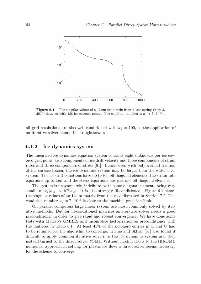
64 Chapter 6. Parallel Direct Sparse Matrix Solvers
0 200 400 600 800 1000
10−5
100
105
Figure 6.1. The singular values of a 12 nm ice matrix from a late spring (May 3,2000) data set with 138 ice covered points. The condition number is κ2 ≈ 7 · 1015.
all grid resolutions are also well-conditioned with κ2 ≈ 100, so the application ofan iterative solver should be straightforward.
6.1.2 Ice dynamics system
The linearized ice dynamics equation system contains eight unknowns per ice cov-ered grid point: two components of ice drift velocity and three components of strainrates and three components of stress [61]. Hence, even with only a small fractionof the surface frozen, the ice dynamics system may be larger than the water levelsystem. The ice drift equations have up to ten off-diagonal elements, the strain rateequations up to four and the stress equations has just one off-diagonal element.
The system is unsymmetric, indefinite, with some diagonal elements being verysmall: maxj |aij | > 106|aii|. It is also strongly ill-conditioned. Figure 6.1 showsthe singular values of an 12 nm matrix from the case discussed in Section 7.2. Thecondition number κ2 ≈ 7 · 1015 is close to the machine precision limit.
On parallel computers large linear system are most commonly solved by iter-ative methods. But for ill-conditioned matrices an iterative solver needs a goodpreconditioner in order to give rapid and robust convergence. We have done sometests with Matlab’s GMRES and incomplete factorization as preconditioner withthe matrices in Table 6.1. At least 45% of the non-zero entries in L and U hadto be retained for the algorithm to converge. Kleine and Sklyar [61] also found itdifficult to apply common iterative solvers to the ice dynamics system and theyinstead turned to the direct solver YSMP. Without modifications to the HIROMBnumerical approach in solving for plastic ice flow, a direct solver seems necessaryfor the scheme to converge.

6.3. Direct sparse matrix solving 65
Residual ‖Ax− b‖2 Max relative differenceGrid Equations Pivoting No pivoting maxi(|xnoi − xpivi |/|xpivi |)12 nm 787 4.0 · 10−11 4.5 · 10−11 4.5 · 10−14
3 nm 16,476 9.2 · 10−10 9.3 · 10−10 3.7 · 10−11
Table 6.1. A comparison of SuperLU dgstrf solutions with partial pivoting(diag pivot thresh = 1.0), and without pivoting (diag pivot thresh = 0.0). Boththe residual and and the differences between the solutions indicate that partial piv-oting is not necessary for these systems.
Lack of diagonal-dominance, indefiniteness, and bad condition number suggestthat partial pivoting would be necessary to reach a correct solution with a directsolver. However, serial HIROMB successfully makes use of the YSMP solver whichdoes no pivoting. We have compared solutions with and without partial pivoting us-ing the direct solver SuperLU [64] in Table 6.1. Both the residuals and the solutiondifferences indicate that pivoting is not needed for these matrices. Furthermore, asthe linear systems originate from Newton iterations of a nonlinear system, an exactlinear solution is not necessary for the iterations to converge to a solution to thenon-linear problem.
6.2 Available solver software
At the start of the parallelization project, there were few direct sparse solversavailable for distributed memory machines. At the time we only had access to asolver written by Bruce Herndon, then at Stanford University [43]. Like the YSMPsolver it handles unsymmetric matrices, and it also does not pivot for stability.Table 6.2 lists a number of other parallel direct sparse solvers for distributed mem-ory of which we are aware1. In addition to Herndon’s solver, the current version ofparallel HIROMB may also use the MUMPS solver [2, 5] from the European PARA-SOL project [4]. Note that the last four packages in the table only do Choleskyfactorization, and thus cannot handle HIROMB’s unsymmetric matrices.
For matrix partitioning we use ParMETIS [55], which is a parallel version ofthe popular METIS package [56] for graph partitioning and fill-reducing matrixreordering. It computes a matrix partitioning which is optimized for parallel fac-torization.
6.3 Direct sparse matrix solving
The solution of a sparse linear equation system with a direct method may be dividedinto four stages:
1Two good sources of free numerical software are the National HPCC Software Exchange(NHSE) at http://www.nhse.org/ and Netlib at http://www.netlib.org/.

66 Chapter 6. Parallel Direct Sparse Matrix Solvers
Solver Comment Ref.Herndon Default solver for HIROMB [43]MUMPS Optional solver for HIROMB [5]SuperLU For distributed memory since 1999 [64]S+ 11 Gflop/s on 128 node T3E-900 [92]SPOOLES Very flexible, but also complex [7]PSPASES Only for symmetric positive definite [38]MP SOLVE Only for symmetric positive definite [19]ScaLAPACK Only for symmetric positive definite [11]PasTiX Only for symmetric positive definite [42]
Table 6.2. Parallel direct sparse matrix solvers available for distributed memorycomputers.
Ordering where the equations are ordered to minimize the fill-in during factor-ization. A good fill-reducing ordering may substantially reduce both compu-tation time and memory use. Multiple minimum degree (MMD) [28] and theNested Dissection (ND) family of algorithms are commonly used. In a paral-lel implementation, the equation ordering is often performed in combinationwith partitioning of the matrix.
Symbolic factorization is based solely on the non-zero structure. In a non-pivoting solver, the fill-in pattern may be completely predicted from thenon-zero structure, and the whole factorization sequence and its memory re-quirements may be precomputed.
Numerical factorization where the actual factorization is computed. If thesolver pivots for stability, the fill-in pattern is dependent on the actual nu-merical values of the matrix elements which complicates parallelization.
Solving phase, where the unknowns are computed with forward and back substi-tution using the computed LU factors.
In HIROMB, the water level matrix remains the same during the whole com-putation, and it needs to be factorized only once at the start of the forecast run.The structure of the ice dynamics matrix may change from one time step to thenext due to freezing and melting, so a new ordering and symbolic factorization isdone in each time step. During the iterations to plastic flow convergence only thevalues of the matrix elements change so that only the numerical factorization andsolve phases are necessary in each iteration.
Herndon’s solver performs all four solution steps in parallel. It accepts any ma-trix partitioning as long as it has the properties of a nested bisection decomposition.For ordering, it uses an MMD algorithm locally on each processor.
MUMPS (version 4.0.3) only parallelizes the two latter numerical factorizationand solve phases. The whole matrix is first transfered to a master processor where

6.3. Direct sparse matrix solving 67
PE 0 PE 1
PE 3PE 2PE 3
PE 0
PE 2
PE 1
Separator level 2Separator level 1 Local equations
Figure 6.2. This example shows how equations generated from a nine pointstencil are classified. Equations on the first half of the PEs that involve equationson the second half are denoted level one separators. Recursively, equations on PE 1involving PE 2 are level two separators as are equations on PE 3 involving PE 4.All other equations are local. Separator equations are shared among the processors.
a fill-reducing ordering is computed using an approximate MMD algorithm [1]. Themaster processor also does the matrix partitioning and symbolic factorization beforethe matrix is distributed back to the remaining processors. MUMPS has the abilityto pivot for stability during the numerical factorization phase, but this is switchedoff in HIROMB.
The ParMETIS package partitions the graph of the matrix in parallel usingmultilevel recursive bisection, an ND algorithm, followed by a MMD ordering locallyin each partition.
6.3.1 Multi-frontal factorization
Both Herndon’s solver and MUMPS make use of the multi-frontal factorizationalgorithm [20]. It is a popular method for imposing order upon a sparse system. Theapproach is an extension of the frontal method first proposed by Irons [53] for finiteelement applications. The multi-frontal method seeks to take a poorly structuredsparse factorization and transform it into a series of smaller dense factorizations.These dense eliminations exhibit a well understood structure and can be made torun well using techniques already developed for dense systems.
In a parallel implementation of the multi-frontal method, the matrix is parti-tioned and distributed onto the participating processors. With a good partitioningmost equations refer only to unknowns on the same processor, and they may be fac-torized independently by each processor. The processors then cooperate to factorizealso the remaining “shared” equations, which involve unknowns on more than oneprocessor. In Herndon’s solver, these shared equations are arranged hierarchicallyinto an elimination tree, where the number of participating processors is halved ateach higher level in the hierarchy, see Figures 6.2 and 6.3. Thus, with a bad par-titioning, where the fraction of shared equations is large, performance may suffer
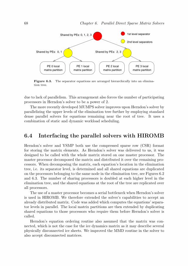
68 Chapter 6. Parallel Direct Sparse Matrix Solvers
Shared by PEs: 0, 1
PE 3 local
Shared by PEs: 2, 3
Shared by PEs: 0, 1, 2, 3
PE 2 localPE 1 localPE 0 localmatrix partition matrix partition matrix partition matrix partition
1st level separator
2nd level separators
Figure 6.3. The separator equations are arranged hierarchically into an elimina-tion tree.
due to lack of parallelism. This arrangement also forces the number of participatingprocessors in Herndon’s solver to be a power of 2.
The more recently developed MUMPS solver improves upon Herndon’s solver byparallelizing the upper levels of the elimination tree further by employing standarddense parallel solvers for equations remaining near the root of tree. It uses acombination of static and dynamic workload scheduling.
6.4 Interfacing the parallel solvers with HIROMB
Herndon’s solver and YSMP both use the compressed sparse row (CSR) formatfor storing the matrix elements. As Herndon’s solver was delivered to us, it wasdesigned to be called with the whole matrix stored on one master processor. Themaster processor decomposed the matrix and distributed it over the remaining pro-cessors. When decomposing the matrix, each equation’s location in the eliminationtree, i.e. its separator level, is determined and all shared equations are duplicatedon the processors belonging to the same node in the elimination tree, see Figures 6.2and 6.3. The number of sharing processors is doubled at each higher level in theelimination tree, and the shared equations at the root of the tree are replicated overall processors.
The use of a master processor becomes a serial bottleneck when Herndon’s solveris used in HIROMB. We therefore extended the solver’s capabilities to accept analready distributed matrix. Code was added which computes the equations’ separa-tor levels in parallel. The local matrix partitions are then extended by duplicatingshared equations to those processors who require them before Herndon’s solver iscalled.
Herndon’s equation ordering routine also assumed that the matrix was con-nected, which is not the case for the ice dynamics matrix as it may describe severalphysically disconnected ice sheets. We improved the MMD routine in the solver toalso accept disconnected matrices.

6.4. Interfacing the parallel solvers with HIROMB 69
100 200 300 400 500 600 700
100
200
300
400
500
600
700
Figure 6.4. The picture on the left shows the ice distribution in the 1 nm grid onMay 3, 2000. About 13% of the grid points (18,251 out of 144,449) were ice covered.The picture on the right shows an example of how this grid would be decomposedinto 74 blocks and distributed onto 16 differently shaded processors.
While the MUMPS solver does both equation ordering and symbolic factor-ization serially, is may still be called with a distributed matrix. This made itstraightforward to interface MUMPS with HIROMB.
6.4.1 Domain decomposition
Since MUMPS computes its own matrix decomposition, it may execute the numer-ical factorization and solve phases in parallel with an optimized load balance, nomatter what the original decomposition might have been. With our extensions,Herndon’s solver accepts and uses the original matrix decomposition directly. Nodata redistribution is necessary before calling the solver. The algorithms for decom-posing HIROMB’s grids into a set of rectangular blocks, as described in Chapter 4also leaves the water level matrix with a good decomposition for Herndon’s solver.But performance will suffer unless the matrix decomposition is load balanced andsuitable for factorization. As is immediately seen in Figure 6.4, the distribution ofthe ice cover is very uneven, making its decomposition in general poorly balanced.
In a further extension to Herndon’s solver, we introduced parallel matrix redis-tribution by calling the routine ParMETIS NodeND from the ParMETIS package [57].Unfortunately ParMETIS, being a graph decomposer, uses an input format differ-ent from the CSR format of the matrix solvers. It was necessary to make the matrixdescription symmetric and to remove all references to diagonal elements before call-ing ParMETIS. ParMETIS also assumes that all processors have a portion of thematrix, and fails to run otherwise. In HIROMB it is almost always the case that

70 Chapter 6. Parallel Direct Sparse Matrix Solvers
Matrix Grid Equations Non-zerosWater level 12 nm 2,171 16,951Ice dynamics 12 nm 1,012 4,969Water level 3 nm 19,073 161,647Ice dynamics 3 nm 16,109 84,073Water level 1 nm 144,449 1,254,609Ice dynamics 1 nm 144,073 762,606
Table 6.3. Matrix sizes fetched from the May 3, 2000 forecast.
some processors are void of ice. This forced us to also even out the initial distribu-tion so that all processors had some part of the matrix before the ParMETIS NodeNDcall.
In the next section we compare the performance of the MUMPS solver withHerndon’s solver, both with and without ParMETIS redistribution.
6.5 Solver performance on CRAY T3E-600
We have measured solver performance on a CRAY T3E-600 and on a SGI Ori-gin 3800 for a set of equation systems from a late spring forecast (May 3, 2000).On this date 13% of the 1 nm grid was ice covered, as shown in Figure 6.4. Table 6.3gives the matrix sizes. Note that ice matrices for the two finer grids have about thesame number of equations as the corresponding water matrices.
We limit the discussion below to the matrices for the two finer grids. Althoughnone of the solvers show decent speedup for the 12 nm grid, the elapsed times arestill insignificant in relation to the time for a whole time step.
6.5.1 Water level system
Figure 6.5 gives times for Herndon’s and MUMPS solvers on the 3 nm system for upto 64 processors of a T3E-600. The upper plot shows that MUMPS is factorizingfive times faster serially, but is overtaken by Herndon on 16 or more processors. Thetime to compute a fill-reducing equation ordering is included under the symbolicfactorization heading. MUMPS does its symbolic factorization phase serially whichaccounts for the mediocre speedup. However, HIROMB’s total performance onlydepends on the solve phase, as the water level matrices are only factorized once perforecast run. The solve times are given in the lower diagram of Figure 6.5. Here,Herndon’s solver is always faster than MUMPS, with the difference increasing forlarger number of processors.
Figure 6.6 shows timings for the larger 1 nm matrix on a T3E-600. Due tomemory limitations at least 8 processors was required to generate the matrix. Here,Herndon’s solver is better in all cases, and always does the solve phase at least three

6.5. Solver performance on CRAY T3E-600 71
1 2 4 8 16 32 640
2
4
6
8
10
12
14
Number of processors
Ela
psed
tim
e
(sec
onds
)
Factorize and solve water level matrix once
Miscellaneous Solve Numeric factorize Symbolic factorize
1 2 4 8 16 32 640
0.05
0.1
0.15
0.2
0.25
Number of processors
Ela
psed
tim
e
(sec
onds
)
Total for one HIROMB time step
Figure 6.5. The upper graph gives times factorizing and solving the water levelmatrix from the 3 nm grid. The left bars show times for MUMPS, and the rightbars show times for Herndon. This matrix is factorized once, and only solved for anew right-hand side in each time step. The time per time step is given in the lowergraph.

72 Chapter 6. Parallel Direct Sparse Matrix Solvers
8 16 32 640
5
10
15
20
25
30
35
40
45
50
Number of processors
Ela
psed
tim
e
(sec
onds
)
Factorize and solve water level matrix once
Miscellaneous Solve Numeric factorize Symbolic factorize
8 16 32 640
0.1
0.2
0.3
0.4
0.5
0.6
0.7
0.8
0.9
1
Number of processors
Ela
psed
tim
e
(sec
onds
)
Total for one HIROMB time step
Figure 6.6. The upper graph gives times factorizing and solving the water levelmatrix from the 1 nm grid. The left bars show times for MUMPS, and the rightbars show times for Herndon. This matrix is factorized once, and only solved for anew right-hand side in each time step. The time per time step is given in the lowergraph.

6.5. Solver performance on CRAY T3E-600 73
times faster than MUMPS. We conclude that Herndon’s solver is the best choicefor both water level matrices on all numbers of processor.
6.5.2 Ice dynamics system
For the ice dynamics matrices, the factorization time becomes important for thetotal runtime, whereas only the solve phase was relevant for the water level matrices.
In the forecast from May 3, 2000, on average 3.1 iterations were necessaryto reach convergence of the nonlinear system in each time step. The number ofiterations were almost the same for both the 3 nm and 1 nm grids. In order toestimate all time spent in the linear solver, the times for numerical factorizationand solve phases should be multiplied by the mean number of iterations.
The time to factorize and solve the 3 nm ice matrix once on a T3E-600 is shownin the upper graph of Figure 6.7, with the average time for a whole time step below.The graphs show that the MUMPS solver is the best alternative for all processorcounts up to 16. For 32 processors and above Herndon’s solver combined withParMETIS redistribution gives a slightly better performance.
Figure 6.8 gives the corresponding timings for the 1 nm grid where the matrixis 9 times larger than for the 3 nm grid. Here the MUMPS and Herndon solversgive about equal performance on one processor with the symbolic factorization ac-counting for more than a third of the total time, but only Herndon with ParMETISgives good speedup on more processors.
The reason for the differing times and speedups between the solvers is clearlyrevealed in Figure 6.9. Here a time line of each processor’s activity is shown usingthe VAMPIR tracing tool [73]. MUMPS is slowest because it does not parallelizesymbolic factorization which accounts for most of the elapsed time. Herndon’ssolver is faster because it parallelizes all solution phases. But it suffers from badload balance as the matrix is only distributed over those processors that happento have the ice covered grid points. By redistributing the matrix with ParMETISbefore calling Herndon’s solver, all processors can take part in the computationwhich substantially improves performance.
6.5.3 ParMETIS optimizations
Initially ParMETIS had low speedup and long execution times. For the 1 nm matrixin Table 6.3, the call to ParMETIS took 5.9 seconds with 32 processors. The localordering within ParMETIS is redundant as Herndon’s solver has its own MMDordering step. By removing local ordering from ParMETIS, the time was reducedto 5.0 seconds and another 0.7 seconds was also cut from the solver’s own orderingtime.
HIROMB originally numbered the ice drift equations first, then the strain rateequations and finally the stress equations, see Figure 6.10. This meant that equa-tions belonging to the same grid point would end up far away in the matrix. Renum-bering the equations so that all equations belonging to a grid point are held together

74 Chapter 6. Parallel Direct Sparse Matrix Solvers
1 2 4 8 16 32 640
1
2
3
4
5
6
7
Number of processors
Ela
psed
tim
e
(sec
onds
)Factorize and solve ice matrix once
Miscellaneous Solve Numeric factorize Symbolic factorizeParMETIS
1 2 4 8 16 32 640
1
2
3
4
5
6
7
Number of processors
Ela
psed
tim
e
(sec
onds
)
Average for one HIROMB time step
Figure 6.7. The upper graph gives times factorizing and solving the ice matrixfrom the 3 nm grid on a T3E-600. The left bar show times for MUMPS, the middlebar Herndon’s solver and the right Herndon with ParMETIS redistribution. Ineach time step this matrix is symbolically factorized once and is then numericallyfactorized and solved in each iteration until convergence. The lower graph gives timesper time step, corresponding to the average number of iterations, which was 3.1 forthis forecast. (A time for Herndon’s solver without ParMETIS on 64 processors ismissing.)

6.5. Solver performance on CRAY T3E-600 75
1 2 4 8 16 32 640
10
20
30
40
50
60
70
80
90
Number of processors
Ela
psed
tim
e
(sec
onds
)Factorize and solve ice matrix once
Miscellaneous Solve Numeric factorize Symbolic factorizeParMETIS
1 2 4 8 16 32 640
10
20
30
40
50
60
70
80
90
Number of processors
Ela
psed
tim
e
(sec
onds
)
Average for one HIROMB time step
Figure 6.8. The upper graph gives times factorizing and solving the ice matrixfrom the 1 nm grid on a T3E-600. The left bar show times for MUMPS, the middlebar Herndon’s solver and the right Herndon with ParMETIS redistribution. Ineach time step this matrix is symbolically factorized once and is then numericallyfactorized and solved in each iteration until convergence. The lower graph givestimes per time step, corresponding to the average number of iterations, which was3.1 for this forecast. (The time for Herndon’s solver with ParMETIS on 1 processoris missing due to memory constraints.)

76 Chapter 6. Parallel Direct Sparse Matrix Solvers
Figure 6.9. VAMPIR traces of MUMPS (top), Herndon (middle) and Hern-don with ParMETIS (bottom) when solving the 1 nm grid ice matrix from the May3, 2000 dataset on 16 processors. Light gray (with texts assemble, cdmford, 106,107, and 109) represents active time spent in the solver and dark gray (MPI Bcast,MPI Allreduce, MPI Send, and MPI Recv) is wasted waiting time due to load imbal-ance. Initialization shown in medium gray to the left is not part of the solver time.Compare with Figure 6.8, upper part.
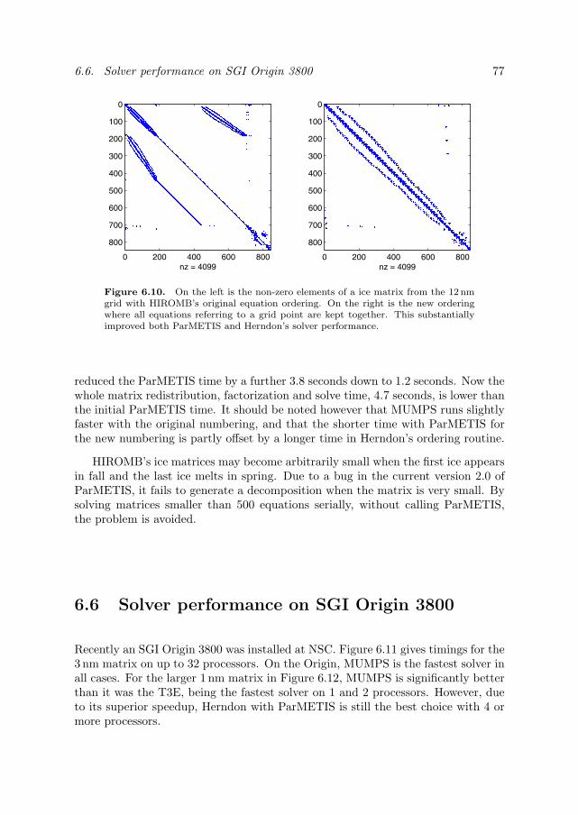
6.6. Solver performance on SGI Origin 3800 77
0 200 400 600 800
0
100
200
300
400
500
600
700
800
nz = 40990 200 400 600 800
0
100
200
300
400
500
600
700
800
nz = 4099
Figure 6.10. On the left is the non-zero elements of a ice matrix from the 12 nmgrid with HIROMB’s original equation ordering. On the right is the new orderingwhere all equations referring to a grid point are kept together. This substantiallyimproved both ParMETIS and Herndon’s solver performance.
reduced the ParMETIS time by a further 3.8 seconds down to 1.2 seconds. Now thewhole matrix redistribution, factorization and solve time, 4.7 seconds, is lower thanthe initial ParMETIS time. It should be noted however that MUMPS runs slightlyfaster with the original numbering, and that the shorter time with ParMETIS forthe new numbering is partly offset by a longer time in Herndon’s ordering routine.
HIROMB’s ice matrices may become arbitrarily small when the first ice appearsin fall and the last ice melts in spring. Due to a bug in the current version 2.0 ofParMETIS, it fails to generate a decomposition when the matrix is very small. Bysolving matrices smaller than 500 equations serially, without calling ParMETIS,the problem is avoided.
6.6 Solver performance on SGI Origin 3800
Recently an SGI Origin 3800 was installed at NSC. Figure 6.11 gives timings for the3 nm matrix on up to 32 processors. On the Origin, MUMPS is the fastest solver inall cases. For the larger 1 nm matrix in Figure 6.12, MUMPS is significantly betterthan it was the T3E, being the fastest solver on 1 and 2 processors. However, dueto its superior speedup, Herndon with ParMETIS is still the best choice with 4 ormore processors.

78 Chapter 6. Parallel Direct Sparse Matrix Solvers
1 2 4 8 16 320
0.5
1
1.5
Number of processors
Ela
psed
tim
e
(sec
onds
)
Factorize and solve ice matrix once
Miscellaneous Solve Numeric factorize Symbolic factorizeParMETIS
1 2 4 8 16 320
0.5
1
1.5
Number of processors
Ela
psed
tim
e
(sec
onds
)
Average for one HIROMB time step
Figure 6.11. The upper graph gives times factorizing and solving the ice matrixfrom the 3 nm grid on a SGI Origin 3800. The left bar show times for MUMPS, themiddle bar Herndon’s solver and the right Herndon with ParMETIS redistribution.In each time step this matrix is symbolically factorized once and is then numericallyfactorized and solved in each iteration until convergence. The lower graph givestimes per time step, corresponding to the average number of iterations, which was3.1 for this forecast.

6.6. Solver performance on SGI Origin 3800 79
1 2 4 8 16 320
5
10
15
20
25
Number of processors
Ela
psed
tim
e
(sec
onds
)Factorize and solve ice matrix once
Miscellaneous Solve Numeric factorize Symbolic factorizeParMETIS
1 2 4 8 16 320
5
10
15
20
25
Number of processors
Ela
psed
tim
e
(sec
onds
)
Average for one HIROMB time step
Figure 6.12. The upper graph gives times factorizing and solving the ice matrixfrom the 1 nm grid on a SGI Origin 3800. The left bar show times for MUMPS, themiddle bar Herndon’s solver and the right Herndon with ParMETIS redistribution.In each time step this matrix is symbolically factorized once and is then numericallyfactorized and solved in each iteration until convergence. The lower graph givestimes per time step, corresponding to the average number of iterations, which was3.1 for this forecast.

80 Chapter 6. Parallel Direct Sparse Matrix Solvers
Solver SGI Cache reuse SGI Cache hit ratio Total time (sec)Level 1 Level 2 Level 1 Level 2 SGI T3E
Herndon 10.3 14.7 91.1% 93.4% 12.7 64.4MUMPS 13.0 49.7 92.8% 98.0% 7.3 69.3
Table 6.4. Cache line reuse and cache line hit ratio when solving the 1 nm matrixin Table 6.3 on one processor of a SGI-3800. Elapsed times on SGI-3800 and T3E-600is also given for reference.
Cache performance data gathered with the SGI perfex tool is given in Table 6.4.The data indicates that MUMPS’ better performance relative to Herndon’s solveron Origin is related to better cache utilization. The MIPS R14000 processors of theOrigin 3800 has a 8 kbyte level 1 cache and 8192 kbyte level 2 cache. Both solversshow similar utilization of level 1 cache, but MUMPS is making better use of thelevel 2 cache. The Alpha EV-5 processors of the CRAY T3E has much smallercaches than the SGI Origin with 8 kbyte of level 1 and 96 kbyte of level 2. TheT3E’s level 2 cache is roughly of the same size as the MIPS processor’s level 1 cacheand the similar performance of the two solvers on T3E might be related to theirsimilar utilization of the MIPS level 1 cache.
6.7 Other solvers
In Table 6.2 on page 66, the three solvers SuperLU, S+ and SPOOLES are alsopossible candidates for use in HIROMB. Amestoy et. al. [3] compared MUMPSwith SuperLU on a CRAY T3E-900 up to 512 processors. SuperLU often usesless memory and scales better, and MUMPS is usually faster on smaller numberof processors. However, they also found that SuperLU spends more time on thesymbolic factorization phase than MUMPS. Like MUMPS this phase is done onjust one processor which limits SuperLU’s suitability for HIROMB.
The S+ solver from UCSB has reached a record breaking 11 Gflop/s sustainedperformance on a 128 processor CRAY T3E-900 [92]. Unfortunately we have notachieved similar performance for neither the water level nor the ice dynamics ma-trices in HIROMB. On both T3E and SGI S+ is close to a magnitude slower thanboth MUMPS and Herndon serially and has low parallel speedup too.
SPOOLES is an object-oriented sparse matrix library with a flexible but alsocomplex solver interface. Like Herndon’s solver, it does the symbolic factorizationphase in parallel. An evaluation of SPOOLES’ performance on HIROMB’s matricesremains future work.
6.8. Conclusion 81
6.8 Conclusion
The ice dynamics model used in HIROMB requires an efficient direct sparse solverin order to make operational 1 nm forecasts feasible. The performance achieved withHerndon’s solver and ParMETIS was absolutely essential on the CRAY T3E-600.The May 3, 2000 forecast with 13% ice coverage would with the MUMPS solverhave taken 6.8 hours on 33 processors. Using Herndon’s solver with ParMETIS theforecast was computed in 1.8 hours. The difference between the solvers grows evenlarger with more ice coverage.
Since August 2001, SMHI’s operational HIROMB forecasts run on 33 processorsof a SGI Origin 3800. The water model (barotropic and baroclinic) accounts forabout 5 seconds per time step. A full summer (ice free) 48-hour forecast is computedin 24 minutes with a time step of 10 minutes. On the SGI the difference in timebetween the MUMPS solver and Herndon/ParMETIS solver is not so large for theMay 3, 2000 example. It is computed in 58 minutes with MUMPS, and in 36minutes with Herndon’s solver and ParMETIS.

82

Chapter 7
Overall Parallel Performance
The main objective for parallelizing HIROMB is the ability to increase grid reso-lution and forecast length within the same runtime as before. Today 33 processorsof an SGI Origin 3800 are used operationally to compute a 48-hour 1 nm forecastwith output every hour in 23 minutes during the ice free season. This is about thesame time (20 minutes) as a 12-hour 3 nm forecast with output every third hourwas computed serially on a Cray C90 in 1997.
In winter season, runtime is highly dependent on the number of ice covered gridpoints. As discussed in Chapters 5 and 6, computation time for ice dynamics isdetermined by the size of the matrix to be factorized in each time step. Figure 7.1shows elapsed runtimes and matrix sizes for operational forecasts during a timeperiod from September 25, 2000 to April 10, 2002. The times are for 33 processorsof a Cray T3E-600, which since early 2001 has served as a backup for the SGIOrigin. With the same number of processors, the T3E-600 runs an ice-free forecastin just over an hour. But in the winter of 2001 runtimes exceeded 4 hours whenabout half the 1 nm grid was covered with ice. The largest ice matrix exceeded500,000 equations on March 19 2001. In the milder winter of 2002 wall clock timeon T3E stayed below 3 hours.
7.1 Parallel speedup
Table 7.1 shows runtime per step and speedup for HIROMB’s three grid sizes onSGI Origin 3800. Both finer grids (3 nm and 1 nm) have close to perfect speedupup to 16 processors and good speedup (26 times) on 32 processors. Figure 7.2illustrates the speedup graphically. The speedup for the coarse 12 nm grid dropsoff with more than 8 processors. The coarser grids does not affect the speedup fora full time step, which is dominated by the 1 nm grid on all numbers of processors.
Corresponding measurements on Cray T3E-600 are given in Table 7.2. Thedistributed memory architecture of the T3E with at most 256 Mbyte available per
83
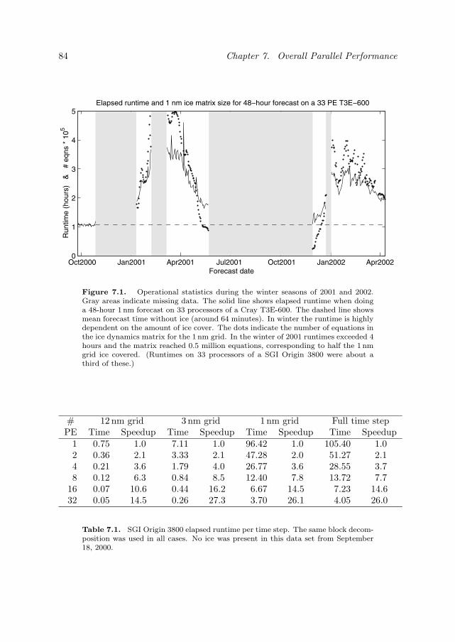
84 Chapter 7. Overall Parallel Performance
Oct2000 Jan2001 Apr2001 Jul2001 Oct2001 Jan2002 Apr20020
1
2
3
4
5
Forecast date
Run
time
(hou
rs)
&
# eq
ns *
105
Elapsed runtime and 1 nm ice matrix size for 48−hour forecast on a 33 PE T3E−600
Figure 7.1. Operational statistics during the winter seasons of 2001 and 2002.Gray areas indicate missing data. The solid line shows elapsed runtime when doinga 48-hour 1 nm forecast on 33 processors of a Cray T3E-600. The dashed line showsmean forecast time without ice (around 64 minutes). In winter the runtime is highlydependent on the amount of ice cover. The dots indicate the number of equations inthe ice dynamics matrix for the 1 nm grid. In the winter of 2001 runtimes exceeded 4hours and the matrix reached 0.5 million equations, corresponding to half the 1 nmgrid ice covered. (Runtimes on 33 processors of a SGI Origin 3800 were about athird of these.)
# 12 nm grid 3 nm grid 1 nm grid Full time stepPE Time Speedup Time Speedup Time Speedup Time Speedup
1 0.75 1.0 7.11 1.0 96.42 1.0 105.40 1.02 0.36 2.1 3.33 2.1 47.28 2.0 51.27 2.14 0.21 3.6 1.79 4.0 26.77 3.6 28.55 3.78 0.12 6.3 0.84 8.5 12.40 7.8 13.72 7.7
16 0.07 10.6 0.44 16.2 6.67 14.5 7.23 14.632 0.05 14.5 0.26 27.3 3.70 26.1 4.05 26.0
Table 7.1. SGI Origin 3800 elapsed runtime per time step. The same block decom-position was used in all cases. No ice was present in this data set from September18, 2000.

7.1. Parallel speedup 85
1 2 4 8 16 3212
4
8
16
32Parallel speedup on SGI Origin 3800
Processors
Spe
edup
1 nm grid 3 nm grid12 nm grid
Figure 7.2. Parallel speedup for HIROMB’s three grid resolutions on SGI Origin3800, based on the data in Table 7.1.
# 12 nm grid 3 nm grid 1 nm grid Full time stepPE Time Speedup Time Speedup Time Speedup Time Speedup
1 2.87 1.0 — — — — — —2 1.54 1.9 11.22 1.0 — — — —4 0.83 3.5 5.80 1.9 — — — —8 0.51 5.6 3.05 3.7 — — — —
16 0.26 11.4 1.46 7.7 17.40 1.0 19.19 1.032 0.20 14.4 0.91 12.3 10.70 1.6 11.87 1.6
Table 7.2. Cray T3E-600 elapsed runtime per time step. The larger grids couldnot be run on low numbers of processors due to lack of memory. No ice was presentin this data set from September 18, 2000.

86 Chapter 7. Overall Parallel Performance
# Grid resolutionPE 12 nm 3 nm 1 nm
1 1 1 12 1.01 1.04 1.004 1.05 1.12 1.048 1.09 1.08 1.03
16 1.22 1.08 1.0932 1.33 1.21 1.11
Table 7.3. SGI Origin 3800 average load balance for a 3-hour forecast (18 steps).The 12 nm grid was decomposed into 71 blocks, the 3 nm grid into 87 blocks, andthe 1 nm grid into 154 blocks.
processor made it necessary to use at least 2 processors for the 3 nm grid, and 16processors for the 1 nm grid.
Speedup is sensitive to domain decomposition quality, see discussion in Chap-ter 4. A high fraction of water points in the decomposition (block efficiency) andgood load balance reduce runtime. To achieve an accurate load balance the de-composition algorithm should use a performance model adapted to the target ar-chitecture. We used two 32-processor decompositions for all timings in Tables 7.1and 7.2, one optimized for Cray T3E and the other for SGI Origin. For the 16processor runs, the processor assignments were combined in pairs (1 & 2 to 1, 3& 4 to 2 etc.). On 8 processors they were combined in groups of four and so on.The block efficiency was therefore the same for all processor counts. Table 7.3 givesmeasured load balance for the SGI timings in Table 7.1. The dominating 1 nm gridhad an average load balance of 1.11 on 32 processors.
7.2 Analysis of a time step
Figure 1.2 on page 6 shows a time line of each processor’s activity during one fulltime step produced by the VAMPIR tracing tool [73] on 17 Cray T3E processors.1
The data is from the May 5 2000 forecast with 13% of the 1 nm grid ice covered, seeFigure 6.4 on page 69. Such traces are good for analyzing the behavior of a parallelprogram and they are especially effective for pinpointing problem areas like hotspots, load imbalances etc. The different parts of the time step is briefly discussedbelow.
1Note that due to a bug in VAMPIR on T3E, the time line at the top of Figures 1.2 and 7.3runs 4 times too fast when compared with Table 7.2.

7.2. Analysis of a time step 87
Coarse grids
The first 10% of the time in Figure 1.2 is spent on the two coarse (12 nm and 3 nm)grids, which provide boundary conditions to the 1 nm grid. Roughly the samenumber of messages (black lines) are transmitted for all grid resolutions and it wasfeared that a high communication overhead and low speedup for the coarse gridswould impact the runtime of the whole forecast. This has not been the case as canbe seen in Tables 7.1 and 7.2. The coarse grids stay around 10% of the total timefor all processor counts on both Cray T3E and SGI Origin.
Barotropic and baroclinic parts
The two most time consuming routines in HIROMB’s water model are flux andtflow. Flux, shown in orange on page 6, solves the continuity and momentumequations. Tflow, in purple, performs advection and diffusion of salinity and tem-perature. In serial HIROMB the total water model time was dominated by tflow,but algorithm improvements and and increased number of flux substeps for the1 nm grid has made flux the most time consuming routine in parallel HIROMB.
Six flux substeps are taken for the 1 nm grid, and Figure 7.3 shows a time linefor one of them. Computations are interspersed with interprocessor communicationfor updating block boundaries. At time 51.2 s in the trace, Herndon’s solver is calledto solve the Helmholtz equation for the water surface level. Only back substitutionis necessary and the solver time is insignificant in relation to the whole time step.
Ice dynamics
In the trace in Figure 1.2 about 50% of the total time is spent on ice dynamics. Theice cover is in this case spread over 3 processors, and all other processors are idle(red) while the ice matrix is assembled (turquoise) and before ParMETIS (green)is called. ParMETIS is used to redistribute the matrix over all processors beforeHerndon’s solver (yellow) is called. 95% of the ice dynamics time is spent insidethe matrix solver (yellow and green). The matrix solver performance is furtheranalyzed in Chapter 6.
Parallel overhead
On both Cray T3E and SGI Origin, direct interprocessor communication is an in-significant part of the total runtime. The delays visible in, for instance, Figure 7.3 isfrom wait-on-receive losses due to load imbalance. HIROMB’s routine for updatingblock boundaries, ExchangeBoundaries (see Chapter 3), uses nonblocking bufferedsends combined with regular receives. If the receiving processor is ready when themessage is sent, the communication time itself is minimal.

88Chapter
7.OverallParallelPerform
ance
Figure 7.3. Time line plot of one flux substep, enlarged from Figure 1.2 on page 6.

7.3. Conclusions and further work 89
For an operational 48-hour forecast on 33 SGI Origin processors, the time forExchangeBoundaries varied between 108 and 398 seconds, or 8% to 29% of an ice-free runtime. The variation between processors is due to load imbalance. Similarrelations have been measured on the Cray T3E.
7.3 Conclusions and further work
With the parallel version of HIROMB, SMHI has been able to track the ongoingdevelopments in computer architecture and produce increasingly longer and finerresolved forecasts of the conditions in the Baltic Sea.
In order to further decrease the forecast runtime, improvements can be madein domain decomposition, with multi-constraint partitioning being a promising op-tion, see Chapter 4. In the author’s opinion, a comparison between HIROMB’scurrent ice dynamics model [61] and the explicitly solved EVP model of Hunke andDukowicz [46, 47] should also be carried out, see Chapter 5.

90
Appendix A
Fundamental Equations
This appendix summarizes the main equations of the HIROMB model. A moredetailed description is available in manuscript [27].
A.1 Momentum balance and continuity
Horizontal momentum balance
Du
Dt− tanφ
Ruv +
1Ruw − tanφ
Ru′v′ +
1Ru′w′
+1
R cosφ
(∂
∂λ(u′u′) +
∂
∂φ(cosφu′v′) +
∂
∂z(R cosφu′w′)
)
= fv − 1
1R cosφ
∂p
∂λ,
(A.1)
Dv
Dt+
tanφR
uu +1Rvw +
tanφR
u′u′ +1Rv′w′
+1
R cosφ
(∂
∂λ(v′u′) +
∂
∂φ(cosφ v′v′) +
∂
∂z(R cosφ v′w′)
)
= −fu− 1
1R
∂p
∂φ,
(A.2)
where the total derivative is
D
Dt=
∂
∂t+
u
R cosφ∂
∂λ+
v
R
∂
∂φ+ w
∂
∂z. (A.3)
Vertical momentum balance (the hydrostatic approximation)
0 = g +1
∂p
∂z. (A.4)
91

92 Appendix A. Fundamental Equations
Equation of continuity (the Boussinesq approximation)
1R cosφ
(∂u
∂λ+∂(cosφv)
∂φ
)+∂w
∂z= 0. (A.5)
Budget of heat
DT
Dt+
1R cosφ
(∂u′T ′
∂λ+∂(cosφv′T ′)
∂φ
)+∂w′T ′
∂z= 0. (A.6)
Budget of salt
DS
Dt+
1R cosφ
(∂u′S′
∂λ+∂(cosφv′S′)
∂φ
)+∂w′S′
∂z= 0. (A.7)
Equation of state according to UNESCO
= (S, T, p). (A.8)
A.2 Turbulence closure
Depending on the large difference in scales between the horizontal and verticalmotion in the ocean, the eddy viscosity for horizontal motion is several orders ofmagnitude greater than the vertical one.
A.2.1 Horizontal momentum flux
In the horizontal, the approach by Smagorinsky [95] is used. Denoting the horizontaleddy viscosity by Kh, the horizontal stresses can be expressed as
−u′u′ = KhDt − k, (A.9)
−u′v′ = KhDs, (A.10)
−v′v′ = −KhDt − k, (A.11)
where Dt denotes the horizontal stretching rate
Dt =1
R cosφ∂u
∂λ− 1R
∂v
∂φ− tanφ
Rv, (A.12)
Ds denotes the horizontal shearing deformation
Ds =1R
∂u
∂φ+
tanφR
u +1
R cosφ∂v
∂λ, (A.13)
and k the fluctuating part of the horizontal kinetic energy
k = (u′u′ + v′v′)/2. (A.14)
A.2. Turbulence closure 93
The horizontal eddy viscosity may then be expressed as
Kh = L2hD (A.15)
where Lh is a horizontal length scale and D denotes an invariant of the deformationrate tensor
D =√D2s + D2
t . (A.16)
For the length scale we use the formula by Smagorinsky
L2h = (κR cosφ∆λ) · (κR∆φ) (A.17)
where κ = 0.4. For the eddy diffusivity we simply use the formula Mh = Kh.
A.2.2 Vertical momentum flux
The shear stress terms (vertical flux of horizontal momentum) are
−w′u′ = Kv∂u
∂z, (A.18)
−w′v′ = Kv∂v
∂z(A.19)
and in analogy with the horizontal mixing, the vertical eddy viscosity is defined as
Kv = L2vψ (A.20)
where Lv is a vertical length scale and ψ is defined as
ψ =
√(∂u
∂z
)2
+(∂v
∂z
)2
(A.21)
In its present version, HIROMB makes use of a diagnostic formula for eddy viscositybased on diagnosed length scale and time scale. To arrive at a formula for thevertical turbulent length scale, we first introduce the flux Richardson number
Rif = − gρ′w′
ρ(u′w′ ∂u
∂z + v′w′ ∂v∂z
) , (A.22)
the gradient Richardson number
Rig = − gρzρψ2
, (A.23)
and the turbulent Prandtl number
Pr =RigRif
=KvMv
. (A.24)
94 Appendix A. Fundamental Equations
The turbulence model by Mellor and Yamada [71] gives a functional dependencebetween Pr and Rig
Pr =Rig
0.725(Rig + 0.186 −√Ri2g − 0.316 Rig + 0.0346)
. (A.25)
From this it follows that
Rif = Rif (Rig) =1Pr
Rig. (A.26)
For the length scale, a generalization of the von Karman formula proposed byLaikhtman [63] is used,
L = κψ(1 − 4 Rif )
| ∂∂z (ψ(1 − 4 Rif ))|. (A.27)
In case of strong variations in the length scale, a smoothing procedure has beenadded. Then, the effective length scale Lv comes from the relaxation equation
dLvdt
= ψ(L− Lv). (A.28)
In this way, a similar equation for the vertical eddy viscosity is constructed,
∂
∂tKv =
ψ
4(Lvϕ−Kv). (A.29)
A.2.3 Tracer mixing
The Reynolds stress terms for tracers are defined analogous to the momentum stressterms
−u′T ′ = Mh1
R cosφ∂T
∂λ(A.30)
−v′T ′ = Mh1R
∂T
∂φ(A.31)
−w′T ′ = Mv∂T
∂z(A.32)
−u′S′ = Mh1
R cosφ∂S
∂λ(A.33)
−v′S′ = Mh1R
∂S
∂φ(A.34)
−w′S′ = Mv∂S
∂z(A.35)
A.3. Forcing and boundary conditions 95
A.2.4 Non-local turbulence
For any z along the vertical, −H ≤ z ≤ ζ, consider the following integral expressions
Ldv(z) = 2κ∫ H+z
0
exp(−∫ z
z−δ
κ dξ
L(ξ)
)dδ, (A.36)
Luv (z) = 2κ∫ ζ−z
0
exp
(−∫ z+δ
z
κ dξ
L(ξ)
)dδ, (A.37)
ψd(z) = κ
∫ H+z
0
exp(−∫ z
z−δ
κ dξ
L(ξ)ψ(z − δ)
)dδ, (A.38)
ψu(z) = κ
∫ ζ−z
0
exp
(−∫ z+δ
z
κ dξ
L(ξ)ψ(z + δ)
)dδ. (A.39)
These integrals are based on master distributions of local scales of length L andfrequency ψ and distinguish between upward and downward excursions, hence thesuperscripts u and d. They are constructed to give integral scales of length Lv andvelocity ϕ based on Prandtl’s picture about the action of turbulence in mixing.Consider a parcel of fluid as it undergoes turbulent excursions. During its travel, itis continuously disintegrated. In the sense of Prandtl, mixing length is the statisticaldistance which is traveled through in the process of disintegration. When theformulae are applied to the example of a logarithmic shear layer, it becomes clearhow an upward and downward integral have to be combined:
Lv(z) = min(Ldv(z), Luv (z)), (A.40)
ϕ(z) = max(ϕd(z), ϕu(z)). (A.41)
For HIROMB the Karman-Laikhtman scale (A.27) is inserted for L.
A.3 Forcing and boundary conditions
HIROMB requires input from both an atmospheric and a hydrological model aswell as from an ocean wave model.
A.3.1 Atmospheric forcing
The atmospheric model HIRLAM [39] provides HIROMB with sea level pressure,wind at 10 m height, air temperature and specific humidity at 2 m above surfaceand total cloudiness. These parameters fully control the momentum and the ther-modynamic balance between the sea surface and the atmosphere. These parametersfully control the momentum and thermodynamic balance between the sea surfaceand the atmosphere.
96 Appendix A. Fundamental Equations
The momentum exchange is computed with a drag formula where the dragcoefficient is computed by a linear relation to the 10 m wind
cD = 0.001(0.7 + 0.09W10) (A.42)
where W10 is wind speed in m/s. Ignoring sea ice, the radiation balance can bewritten as
Q = QI + QB + QH + QE (A.43)
where QI , QB , QH and QE stand for short-wave solar radiation, long-wave radia-tion, sensible heat flux and latent heat flux respectively. The Baltic Sea is almostin thermodynamic equilibrium with the atmosphere averaged over a year [77]. Themain contribution comes from the incoming short-wave radiation which as an an-nual mean is in balance with the heat loss terms. The formula for short-waveinsolation is given by Shine [93],
Qi = Q0s2
1.2s + (1 + s)ea + 0.046(1 − 0.6c). (A.44)
Q0 is the solar constant, s the sine of inclination of the sun above the horizon givenby
s = max(sinφ sin δ + cosφ cos δ cosω, 0) (A.45)
where δ is the declination angle of the sun and ω the time angle of the local meridian.QI is then calculated as QI = (1−α)Qi, where α is the albedo of the water surface.The net long-wave radiation is computed with a formula from Idso and Jackson [49],
QB = εσ(T 4a (1 − 0.26 exp(−7.7 · 10−4(Ta − 273)2)(1 − 0.75c2)) − T 4
s ). (A.46)
Here ε is the emissivity of the water surface, σ the Stefan-Boltzmann constant,Ts water temperature, Ta air temperature, ea the water vapor pressure in theatmosphere and c is the cloud coverage ranging from 0 to 1.
The sensible heat flux is driven by the temperature difference between waterand air and is expressed as
QH = cpaacH(Ta − Ts)W10 (A.47)
where cpa is the specific heat of air, air density, and cH a diffusivity constant. Inan analogous way, the latent heat flux is written
QE = LacE(qa − qs)W10 (A.48)
where L is the latent heat of evaporation, qs is specific humidity at sea surface andqa specific humidity at 10 m height.

A.3. Forcing and boundary conditions 97
45
45
50
55
60
65
70
-35
-30
-25
-20
-15
-10
-5 0 5
10
15
20
2530
Figure A.1. The computational grid of the 2D North Atlantic storm surge model.
A.3.2 Open boundary forcing
The coarsest HIROMB grid has an open boundary to the North Atlantic. One partof this boundary line runs through the British Channel, the other makes a straightline between northern Scotland and south-west Norway. Along all that line, waterlevel, salinity and temperature are prescribed at each time step.
Inflow data of salinity and temperature at the open boundary is provided bymonthly climatological fields. In order to relax their influence on the operationalsimulation, there is a sponge layer along the boundary line which acts as a bufferbetween the inner model domain and a “climatological reservoir” outside. It isflushed by the normal flow component as computed along the boundary line. Thisflow either brings a climatological signal or outflow from the interior into the sponge.When flow direction is reversed from outward to inward, it returns what it was filledwith, until, in sustained flow, its capacity is exhausted, and it passes more and moreof the reservoir. Conversely, for outward flow, the sponge empties into the reservoirwhich is thought to be of infinite capacity, i.e. not responding to that input. Theperformance of the sponge is a matter if its capacity. This capacity should besufficiently large not to let the reservoir be felt in tidal reversions, but sufficientlysmall to give an input effect for sustained inflow. There are three different types ofopen boundaries in the model system:
(i) Open boundary around the 2D Atlantic storm surge model area. The compu-tational grid of the 2D North Atlantic model is given in Figure A.1. Its boundariesare aligned with latitude and longitude where a radiation condition is used.
(ii) Open boundary for the coarsest 3D Baltic Sea model to the 2D Atlantic stormsurge model. The boundary values of water level come from two sources. They aresuperposed by the results of a storm surge model for the North Atlantic, which

98 Appendix A. Fundamental Equations
is void of tides, and a setup of 17 tidal constituents, specified for each individualboundary cell. All tidal forcing is supplied at the open boundaries between theNorth Sea and the Atlantic.
(iii) Open boundary between the different nested grids in the Baltic Sea model.The coupling between the nested 3D grids is both of a one-way and a two-waytype. For salinity and temperature, which are solved with an explicit scheme, usetwo-way coupling, whereas the implicitly solved water level is only one-way.
A.3.3 River runoff
A river runoff model [35] covering the entire Baltic drainage basin, Skagerrak andKattegat runs on an operational basis at SMHI. The hydrological model producesas output, daily river runoff for 43 sub-basins of which 8 represents the Skagerrak-Kattegat area, see Figure A.2. A further division of the runoff for each sub-basinis made between the major rivers ending up at a total of 82 rivers.
A.3.4 Ocean wave forcing
From the viewpoint of a filtered model (large scale, slow evolution), waves makea sub-scale process. The presence of waves gives a net effect which comes fromself-correlation. The Stokes drift is a mass flow which originates from correla-tion between surface elevation and flow. In an oscillating wave, forward flow andbackward flow do not exactly cancel out but leave a net flow. In the momentumequations, the quadratic terms also leave a non-vanishing effect on averaging. Thus,although waves are a much faster phenomenon than what a filtered model is de-signed to do, their presence should not be neglected. This is the more necessarythe more intense the waves are, because the filter effect is non-linear with respectto wave characteristics.
Unlike entirely irregular turbulent fluctuations, waves are much more accessibleto modeling. We employ HYPAS (HYbrid PArametric and Shallow) [32], whichis a phase-averaged model describing the comparatively slow evolution of waveenergy quantities. In that model, the entire wave energy spectrum is composedin a hybrid way from wind-sea and swell. Either component is given in a simpleform which depends on only a few parameters. A parameterization is also appliedto the influence of water depth. HYPAS provides what may be considered asthe “wave forcing” for HIROMB. Like the atmospheric model HIRLAM, it is runindependently and in advance of HIROMB.

A.3. Forcing and boundary conditions 99
Skagerak
BalticProper
Gulf of Finland
BothnianBay
BothnianSea
DanishStraits
Kattegat
Gulf ofRiga
Figure A.2. Catchment area with major rivers for the Baltic Sea, Skagerrak andKattegat and the distribution of separate drainage basins (black lines) for which theriver runoff forecast model is run.

100
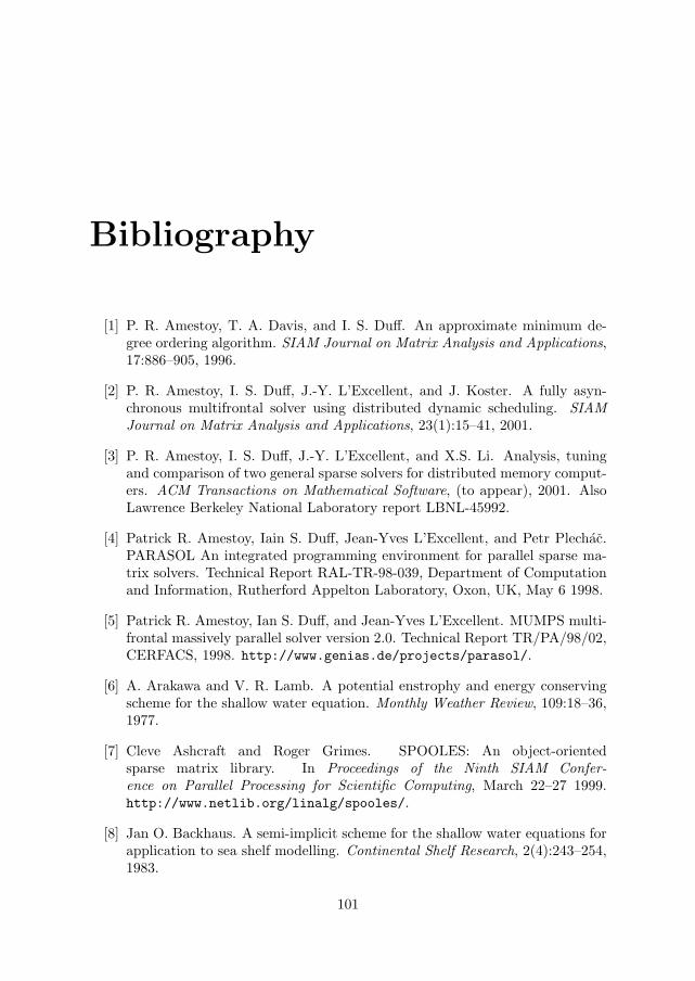
Bibliography
[1] P. R. Amestoy, T. A. Davis, and I. S. Duff. An approximate minimum de-gree ordering algorithm. SIAM Journal on Matrix Analysis and Applications,17:886–905, 1996.
[2] P. R. Amestoy, I. S. Duff, J.-Y. L’Excellent, and J. Koster. A fully asyn-chronous multifrontal solver using distributed dynamic scheduling. SIAMJournal on Matrix Analysis and Applications, 23(1):15–41, 2001.
[3] P. R. Amestoy, I. S. Duff, J.-Y. L’Excellent, and X.S. Li. Analysis, tuningand comparison of two general sparse solvers for distributed memory comput-ers. ACM Transactions on Mathematical Software, (to appear), 2001. AlsoLawrence Berkeley National Laboratory report LBNL-45992.
[4] Patrick R. Amestoy, Iain S. Duff, Jean-Yves L’Excellent, and Petr Plechac.PARASOL An integrated programming environment for parallel sparse ma-trix solvers. Technical Report RAL-TR-98-039, Department of Computationand Information, Rutherford Appelton Laboratory, Oxon, UK, May 6 1998.
[5] Patrick R. Amestoy, Ian S. Duff, and Jean-Yves L’Excellent. MUMPS multi-frontal massively parallel solver version 2.0. Technical Report TR/PA/98/02,CERFACS, 1998. http://www.genias.de/projects/parasol/.
[6] A. Arakawa and V. R. Lamb. A potential enstrophy and energy conservingscheme for the shallow water equation. Monthly Weather Review, 109:18–36,1977.
[7] Cleve Ashcraft and Roger Grimes. SPOOLES: An object-orientedsparse matrix library. In Proceedings of the Ninth SIAM Confer-ence on Parallel Processing for Scientific Computing, March 22–27 1999.http://www.netlib.org/linalg/spooles/.
[8] Jan O. Backhaus. A semi-implicit scheme for the shallow water equations forapplication to sea shelf modelling. Continental Shelf Research, 2(4):243–254,1983.
101

102 Bibliography
[9] Jan O. Backhaus. A three-dimensional model for the simulataion of shelf seadynamics. Deutsche Hydrographische Zeitschrift, 38(4):165–187, 1985.
[10] M. I. Beare and D. P. Stevens. Optimisation of a parallel ocean generalcirculation model. Ann. Geophysicae, 15:1369–1377, 1997.
[11] L.S. Blackford et al. ScaLAPACK Users’ Guide. SIAM, 1997.
[12] R. S. Bleck, M. O’Keefe, and A. Sawdey. A comparaision of data-parallel andmessage-passing versions of the Miami Isopycnic Coordinate Ocean ModelMICOM. Parallel Computing, 21:1695–1720, 1995.
[13] Rainer Bleck. An oceanic general circulation model framed in hybridisopycnic-cartesian coordinates. Ocean Modelling, 4(55–88), 2002.
[14] A. F. Blumberger and G. L. Mellor. A description of a three-dimensionalcoastal ocean circulation model. In N. S. Heaps, editor, Three-DimensionalCoastal Ocean Models, volume 4 of Coastal Estuarine Ser., page 208 pp. AGU,Washington, DC, 1987.
[15] K. Bryan. A numerical method for the study of the circulation of the worldocean. J. Comput. Phys., 4:347–376, 1969.
[16] R. Colony and R. S. Pritchard. Integration of elastic-plastic constitutive laws.AIDJEX Bull., 30:55–80, 1975.
[17] M. D. Coon. A review of AIDJEX modelling. In R. S. Prichard, editor, SeaIce Processes and Models, pages 12–25. University of Washington Press, 1980.
[18] M. D. Coon, S. A. Maykut, R. S. Pritchard, D. A. Rothrock, and A. S.Thorndike. Modeling the pack ice as an elastic-plastic material. AIDJEXBull., pages 1–105, 1974.
[19] William Dearholt, Steven Castillo, Derek Barnes, and Gary Henni-gan. Direct solution of large, sparse systems of equations on a dis-tributed memory computer. Technical report, Klipsch School of Elec-trical and Computer Engineering New Mexico State University, 1999.http://emlab2.nmsu.edu/papers/par_sparse/.
[20] I. S. Duff, A. M. Erisman, and J. K. Reid. Direct Methods for Sparse Matrices.Oxford University Press, 1986.
[21] S. C. Eisenstat, H. C. Elman, M. H. Schultz, and A. H. Sherman. The (new)Yale sparse matrix package. In G. Birkhoff and A. Schoenstadt, editors,Elliptic Problem Solvers II, pages 45–52. Academic Press, 1994.
[22] S. J. Fink, S. R. Kohn, and S. B. Baden. Efficient run-time support for ir-regular block-structured applications. J. Parallel and Distributed Computing,50:61–82, 1998.

Bibliography 103
[23] G. M. Flato and W. D. Hibler III. Modeling pack ice as a cavitating fluid. J.Phys. Oceanogr., 1992.
[24] L. Funkquist. Studies of upwelling in the Baltic Sea with a numerical model.Rapporter Hydrologi och Oceanografi 45, SMHI, SE-601 76 Norrkoping, Swe-den, 1985.
[25] L. Funkquist. An operational Baltic Sea circulation model. Reports Oceanog-raphy 18, SMHI, SE-601 76 Norrkoping, Sweden, 1993.
[26] L. Funkquist and L. Gidhagen. A model for pollution studies in the BalticSea. Rapporter Hydrologi och Oceanografi 39, SMHI, SE-601 76 Norrkoping,Sweden, 1984.
[27] Lennart Funkquist and Eckhard Kleine. An introduction to HIROMB, anoperational baroclinic model for the Baltic Sea. Technical report, SMHI,Norrkoping, Sweden, 200X. In manuscript.
[28] Alan George and Joseph W.-H. Liu. The evolution of the minimum degreeordering algorithm. SIAM Review, 31:1–19, 1989.
[29] R. Gerdes, M. Karcher, J. Brauch, C. Koeberle, and B. Fritzsch. Propa-gation of Atlantic water into the Nordic Seas and in the Actic Ocean inhigh-resolution coupled sea ice-ocean simulations. In preparation, 200X.
[30] Adrian. D. Gill, editor. Atmosphere-Ocean Dynamics. Academic Press, NewYork, 1982.
[31] V. Gulzow and K. Kleese. About the parallelization of the HOPE oceanmodel. In Geerd-R. Hoffman and Norbert Kreitz, editors, Coming of Age,Proceedings of the Sixth ECMWF Workshop on the Use of Parallel Processorsin Meteorology, pages 505–511. World Scientific, 1995.
[32] H. Gunther and W. Rosenthal. Shallow water surface wave model basedon the Texel-Marsen-Arsloe (TMA) wave spectrum. In Proceedings of the20th Congress of the International Association of Hydraulic Research (IAHR),Moscow, 1983.
[33] G. H. Golub and C. F. Van Loan. Unsymmetric positive definite linear sys-tems. Lin. Alg. and Its Applic., 28:85–98, 1979.
[34] M. W. Govett, D. S. Schaffer, T. Henderson, L. B. Hart, J. P. Edwards,C.S. Liou, and T.-L. Lee. SMS: A directive-based parallelization approachfor shared and distributed memory high performance computers. Technicalreport, NOAA Forecast System Laboratory, Boulder, March 2001.
[35] L. Phil Graham. Large-scale hydrological modeling in the Baltic basin. PhDthesis, Division of Hydraulic Engineering, Department of Civil and Environ-mental Engineering, Royal Institute of Technology, Stockholm, Sweden, 2000.
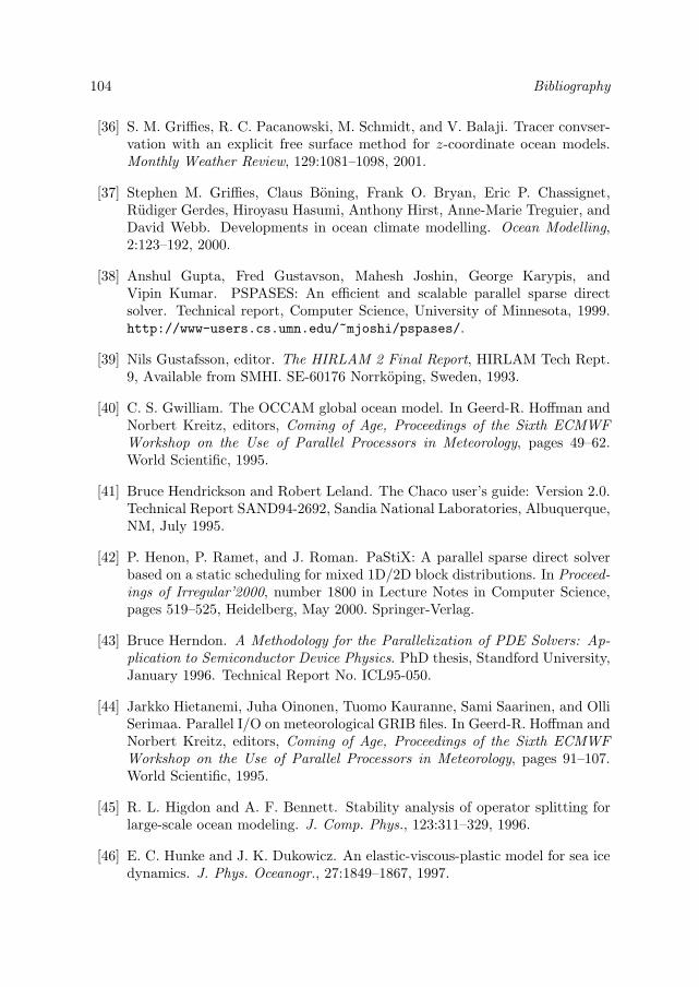
104 Bibliography
[36] S. M. Griffies, R. C. Pacanowski, M. Schmidt, and V. Balaji. Tracer convser-vation with an explicit free surface method for z-coordinate ocean models.Monthly Weather Review, 129:1081–1098, 2001.
[37] Stephen M. Griffies, Claus Boning, Frank O. Bryan, Eric P. Chassignet,Rudiger Gerdes, Hiroyasu Hasumi, Anthony Hirst, Anne-Marie Treguier, andDavid Webb. Developments in ocean climate modelling. Ocean Modelling,2:123–192, 2000.
[38] Anshul Gupta, Fred Gustavson, Mahesh Joshin, George Karypis, andVipin Kumar. PSPASES: An efficient and scalable parallel sparse directsolver. Technical report, Computer Science, University of Minnesota, 1999.http://www-users.cs.umn.edu/~mjoshi/pspases/.
[39] Nils Gustafsson, editor. The HIRLAM 2 Final Report, HIRLAM Tech Rept.9, Available from SMHI. SE-60176 Norrkoping, Sweden, 1993.
[40] C. S. Gwilliam. The OCCAM global ocean model. In Geerd-R. Hoffman andNorbert Kreitz, editors, Coming of Age, Proceedings of the Sixth ECMWFWorkshop on the Use of Parallel Processors in Meteorology, pages 49–62.World Scientific, 1995.
[41] Bruce Hendrickson and Robert Leland. The Chaco user’s guide: Version 2.0.Technical Report SAND94-2692, Sandia National Laboratories, Albuquerque,NM, July 1995.
[42] P. Henon, P. Ramet, and J. Roman. PaStiX: A parallel sparse direct solverbased on a static scheduling for mixed 1D/2D block distributions. In Proceed-ings of Irregular’2000, number 1800 in Lecture Notes in Computer Science,pages 519–525, Heidelberg, May 2000. Springer-Verlag.
[43] Bruce Herndon. A Methodology for the Parallelization of PDE Solvers: Ap-plication to Semiconductor Device Physics. PhD thesis, Standford University,January 1996. Technical Report No. ICL95-050.
[44] Jarkko Hietanemi, Juha Oinonen, Tuomo Kauranne, Sami Saarinen, and OlliSerimaa. Parallel I/O on meteorological GRIB files. In Geerd-R. Hoffman andNorbert Kreitz, editors, Coming of Age, Proceedings of the Sixth ECMWFWorkshop on the Use of Parallel Processors in Meteorology, pages 91–107.World Scientific, 1995.
[45] R. L. Higdon and A. F. Bennett. Stability analysis of operator splitting forlarge-scale ocean modeling. J. Comp. Phys., 123:311–329, 1996.
[46] E. C. Hunke and J. K. Dukowicz. An elastic-viscous-plastic model for sea icedynamics. J. Phys. Oceanogr., 27:1849–1867, 1997.
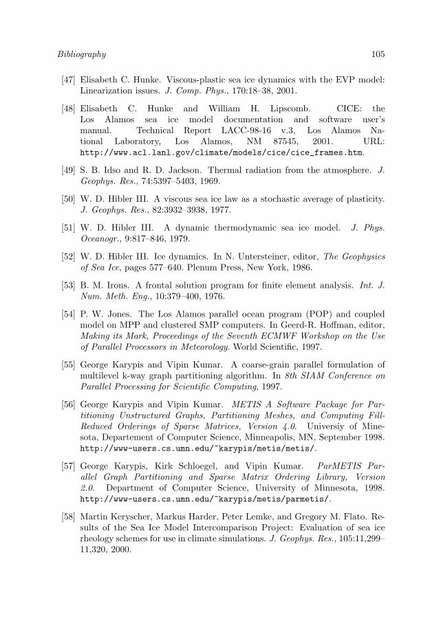
Bibliography 105
[47] Elisabeth C. Hunke. Viscous-plastic sea ice dynamics with the EVP model:Linearization issues. J. Comp. Phys., 170:18–38, 2001.
[48] Elisabeth C. Hunke and William H. Lipscomb. CICE: theLos Alamos sea ice model documentation and software user’smanual. Technical Report LACC-98-16 v.3, Los Alamos Na-tional Laboratory, Los Alamos, NM 87545, 2001. URL:http://www.acl.lanl.gov/climate/models/cice/cice_frames.htm.
[49] S. B. Idso and R. D. Jackson. Thermal radiation from the atmosphere. J.Geophys. Res., 74:5397–5403, 1969.
[50] W. D. Hibler III. A viscous sea ice law as a stochastic average of plasticity.J. Geophys. Res., 82:3932–3938, 1977.
[51] W. D. Hibler III. A dynamic thermodynamic sea ice model. J. Phys.Oceanogr., 9:817–846, 1979.
[52] W. D. Hibler III. Ice dynamics. In N. Untersteiner, editor, The Geophysicsof Sea Ice, pages 577–640. Plenum Press, New York, 1986.
[53] B. M. Irons. A frontal solution program for finite element analysis. Int. J.Num. Meth. Eng., 10:379–400, 1976.
[54] P. W. Jones. The Los Alamos parallel ocean program (POP) and coupledmodel on MPP and clustered SMP computers. In Geerd-R. Hoffman, editor,Making its Mark, Proceedings of the Seventh ECMWF Workshop on the Useof Parallel Processors in Meteorology. World Scientific, 1997.
[55] George Karypis and Vipin Kumar. A coarse-grain parallel formulation ofmultilevel k-way graph partitioning algorithm. In 8th SIAM Conference onParallel Processing for Scientific Computing, 1997.
[56] George Karypis and Vipin Kumar. METIS A Software Package for Par-titioning Unstructured Graphs, Partitioning Meshes, and Computing Fill-Reduced Orderings of Sparse Matrices, Version 4.0. Universiy of Mine-sota, Departement of Computer Science, Minneapolis, MN, September 1998.http://www-users.cs.umn.edu/~karypis/metis/metis/.
[57] George Karypis, Kirk Schloegel, and Vipin Kumar. ParMETIS Par-allel Graph Partitioning and Sparse Matrix Ordering Library, Version2.0. Department of Computer Science, University of Minnesota, 1998.http://www-users.cs.umn.edu/~karypis/metis/parmetis/.
[58] Martin Keryscher, Markus Harder, Peter Lemke, and Gregory M. Flato. Re-sults of the Sea Ice Model Intercomparison Project: Evaluation of sea icerheology schemes for use in climate simulations. J. Geophys. Res., 105:11,299–11,320, 2000.

106 Bibliography
[59] Eckhard Kleine. Die Konzeption eines numerischen Verfarens fur die Advek-tionsgleichung. Technical report, Bundesamt fur Seeschiffahrt und Hydrogra-phie, Hamburg, Germany, 1993.
[60] Eckhard Kleine. Das operationelle Model des BSH fur Nordsee und Ostsee,Konzeption und Ubersicht. Technical report, Bundesamt fur Seeschiffahrtund Hydrographie, Hamburg, Germany, 1994.
[61] Eckhard Kleine and Sergey Sklyar. Mathematical features of Hibler’smodel of large-scale sea-ice dynamics. Deutsche Hydrographische Zeitschrift,47(3):179–230, 1995.
[62] Manu Konchady, Arun Sood, and Paul S. Schopf. Implementation and perfor-mance evaluation of a parallel ocean model. Parallel Computing, 24(181–203),1998.
[63] D. L. Laikhtman. On the structure of the planetary boundary layer. Phys.Atmos. Oceans (russian), 15:983–987, 1979.
[64] Xiaoye S. Li and James W. Demmel. Making sparse Gaussian eliminationscalable by static pivoting. In Supercomputing ’98 Proceedings, 1998. URL:http://www.supercomp.org/sc98/.
[65] P. Lockey, R. Proctor, and I. D. James. Characterization of I/O requirementsin a massively parallel shelf sea model. The International Journal of HighPerformance Computing Applications, 12(3):320–332, 1998.
[66] Phu Luong, Clay P. Breshears, and Le N. Ly. Dual-level parallelism improvesload-balance in coastal ocean circulation modeling. Technical Report TR/00-18, ERDC MSRC/PET, February 2000.
[67] J. Marshall, C. Hill, L. Perelman, and A. Adcroft. Hydrostatic, quasi-hydrostatic and nonhydrostatic ocean modeling. J. Geophys. Res., 102:5733–5752, 1997.
[68] H. E. M. Meier, R. Doscher, A. C. Coward, J. Nycander, and K. Doos. RCO –Rossby Centre regional Ocean climate model: Model description (version 1.0)and first results from the hindcast period 1992/93. Technical Report ReportsOceanography No. 26, Swedish Meteorological and Hydrological Institute,SE-601 76 Norrkoping, Sweden, 1999. 102 pp.
[69] H. E. Markus Meier and Torgny Faxen. Performance analysis of a multipro-cessor coupled ice-ocean model for the Baltic Sea. Journal of Atmosphericand Oceanic Technology, 19(1), 2002.
[70] Verena Meiser, editor. Computational Science Education Project, e-bookOcean Models. Computational Science Education Project, 1995. URL:http://csep1.phy.ornl.gov/CSEP/OM/OM.html.

Bibliography 107
[71] G. L. Mellor and T. Yamada. A hierachy of turbulence closure models forplanetary boundary layers. J. Atmos. Sci., 31:1791–1806, 1974.
[72] Message Passing Interface Forum. MPI-2: Extensions to the Message-PassingInterface, 1997. Available at http://www.mpi-forum.org/.
[73] W. E. Nagel, A. Arnold, M. Weber, H.-C. Hoppe, and K. Solchenbach. VAM-PIR: visualization and analysis of MPI resources. Supercomputer, 12(1):69–90,1996.
[74] J. M. Oberhuber. Simulation of the Atlantic circulation with a coupled sea ice-mixed layer-isopycnal general circulation model. part I: Model experiment. J.Phys. Oceanogr., 23:808–829, 1993.
[75] J. M. Oberhuber and K. Ketelsen. Parallelization of an OGCM on the CRAYT3D. In Geerd-R. Hoffman and Norbert Kreitz, editors, Coming of Age,Proceedings of the Sixth ECMWF Workshop on the Use of Parallel Processorsin Meteorology, pages 494–504. World Scientific, 1995.
[76] Wade. D. Oberpiller, Aaron C. Sawdey, Matthew T. O’Keefe, and ShaobaiGao. Parallelizing the Princeton ocean model using TOPAZ. Technical re-port, Parallel Computer Sys. Lab., Dept. Elec. Comp. Eng., University ofMinnesota, 1999.
[77] A. T. Omstedt and A. Rutgersson. Closing the water and heat cycles of theBaltic Sea. Meteorol. Z., 9:57–64, 2000.
[78] Ronald C. Pacanowski and Stephen M. Griffies. MOM 3.1 Manual.NOAA/Geophysical Fluid Dynamics Laboratory, Princeton, NJ, 2000. 680pp.
[79] R. S. Pritchard. An elastic-plastic constitutive law for sea ice. J. Appl. Mech.,42E:379–384, 1975.
[80] Jarmo Rantakokko. Data Partitioning Methods and Parallel Block-OrientedPDE Solvers. PhD thesis, Uppsala University, 1998.
[81] Jarmo Rantakokko. A framework for partitioining domains with inhomoge-nous workload. Parallel Algorithms and Applications, 13:135–151, 1998.
[82] Jarmo Rantakokko. An integrated decomposition and partitioning approachfor irregular block-structured applications. In J. Rolim et al., editors, IPDPSWorkshops 2000, number 1800 in Lecture Notes in Computer Science, pages485–496, Heidelberg, 2000. Springer-Verlag.
[83] A. Sawdey, M. O’Keefe, R. Bleck, and R. W. Numrich. The design, implemen-tation, and performance of a parallel ocean circulation model. In Geerd-R.Hoffman and Norbert Kreitz, editors, Coming of Age, Proceedings of the Sixth

108 Bibliography
ECMWF Workshop on the Use of Parallel Processors in Meteorology. WorldScientific, 1995.
[84] Aaron C. Sawdey and Matthew T. O’Keefe. A general programming modelfor developing scalable ocean circulation applications. In Geerd-R. Hoffman,editor, Making its Mark, Proceedings of the Seventh ECMWF Workshop onthe Use of Parallel Processors in Meteorology. World Scientific, 1997.
[85] Josef Schule. Heading for an asynchronous parallel ocean model. In RecentAdvances in Parallel Virtual Machine and Message Passing Interface. 6thEuropean PVM/MPI User’s Group Meeting, volume 1697 of Lecture Notes inComputer Science, pages 404–409, Heidelberg, 1999. Springer-Verlag.
[86] Josef Schule and Tomas Wilhelmsson. Parallelizing a high resolution opera-tional ocean model. In P. Sloot, M. Bubak, A. Hoekstra, and B. Hertzberger,editors, High-Performance Computing and Networking, number 1593 in Lec-ture Notes in Computer Science, pages 120–129, Heidelberg, 1999. Springer-Verlag.
[87] A. Semtner. A model for the thermodynamic growth of sea ice in numericalinvestigations of climate. J. Phys. Oceanogr., 6:379–389, 1976.
[88] A. Semtner. Ocean and climate modelling. Communications of the ACM,43(4):81–89, April 2000.
[89] A. J. Semtner and R. M. Chervin. Ocean general circulation from a globaleddy-resolving model. J. Geophys. Res., 97:5493–5550, 1992.
[90] SGI. Application Programmer’s I/O Guide, document number 007-3695-004edition, 1999. Available at http://techpubs.sgi.com/.
[91] A. F. Shchepetkin and J. C. McWilliams. The Regional Ocean ModelingSystem: A split-explicit, free-surface, topography-following coordinates oceanmodel. In draft, URL: http://marine.rutgers.edu/po/models/roms/.
[92] Kai Shen, Tao Yang, and Xiangmin Jiao. S+ efficient 2D sparse LU factor-ization on parallel machines. SIAM Journal on Matrix Analysis and Appli-cations, 22(1):282–305, 2000.
[93] K. P. Shine. Parameterization of shortwave flux over high albedo surfacesas function of cloud thickness and surface albedo. Q. J. R. Meteorol. Soc.,110:747–761, 1984.
[94] Horst D. Simon. Partitioning of unstructured problems for parallel processing.Computing Systems in Engineering, 2:135–148, 1991.
[95] J. Smagorinsky. General circulation experiments with primitive equations, I.The basic experiment. Monthly Weather Review, 91:99–164, 1963.
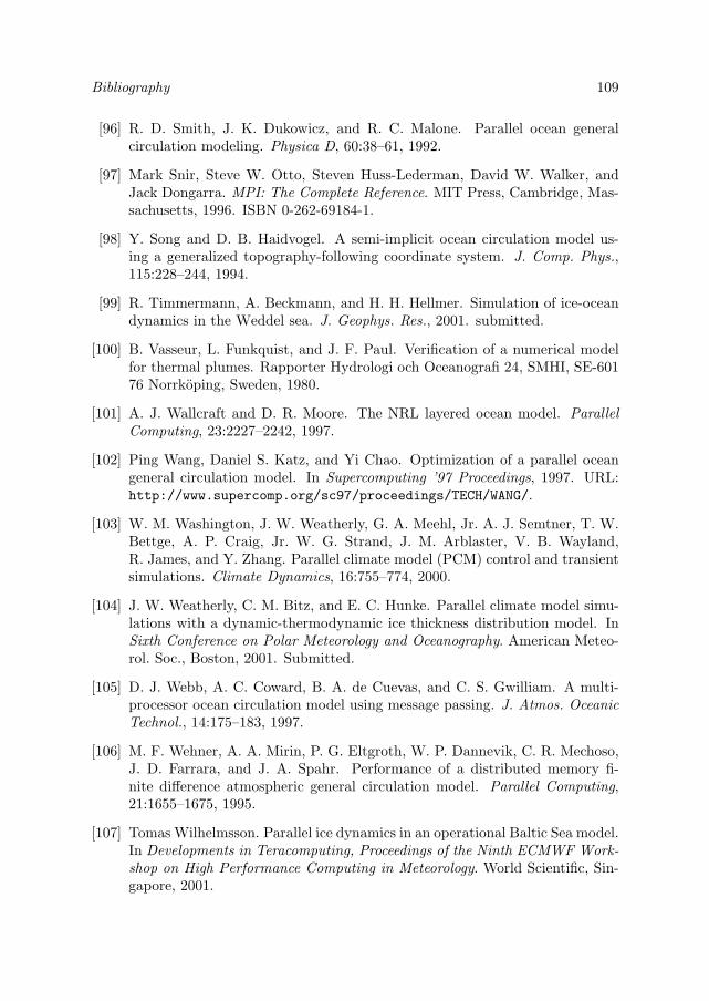
Bibliography 109
[96] R. D. Smith, J. K. Dukowicz, and R. C. Malone. Parallel ocean generalcirculation modeling. Physica D, 60:38–61, 1992.
[97] Mark Snir, Steve W. Otto, Steven Huss-Lederman, David W. Walker, andJack Dongarra. MPI: The Complete Reference. MIT Press, Cambridge, Mas-sachusetts, 1996. ISBN 0-262-69184-1.
[98] Y. Song and D. B. Haidvogel. A semi-implicit ocean circulation model us-ing a generalized topography-following coordinate system. J. Comp. Phys.,115:228–244, 1994.
[99] R. Timmermann, A. Beckmann, and H. H. Hellmer. Simulation of ice-oceandynamics in the Weddel sea. J. Geophys. Res., 2001. submitted.
[100] B. Vasseur, L. Funkquist, and J. F. Paul. Verification of a numerical modelfor thermal plumes. Rapporter Hydrologi och Oceanografi 24, SMHI, SE-60176 Norrkoping, Sweden, 1980.
[101] A. J. Wallcraft and D. R. Moore. The NRL layered ocean model. ParallelComputing, 23:2227–2242, 1997.
[102] Ping Wang, Daniel S. Katz, and Yi Chao. Optimization of a parallel oceangeneral circulation model. In Supercomputing ’97 Proceedings, 1997. URL:http://www.supercomp.org/sc97/proceedings/TECH/WANG/.
[103] W. M. Washington, J. W. Weatherly, G. A. Meehl, Jr. A. J. Semtner, T. W.Bettge, A. P. Craig, Jr. W. G. Strand, J. M. Arblaster, V. B. Wayland,R. James, and Y. Zhang. Parallel climate model (PCM) control and transientsimulations. Climate Dynamics, 16:755–774, 2000.
[104] J. W. Weatherly, C. M. Bitz, and E. C. Hunke. Parallel climate model simu-lations with a dynamic-thermodynamic ice thickness distribution model. InSixth Conference on Polar Meteorology and Oceanography. American Meteo-rol. Soc., Boston, 2001. Submitted.
[105] D. J. Webb, A. C. Coward, B. A. de Cuevas, and C. S. Gwilliam. A multi-processor ocean circulation model using message passing. J. Atmos. OceanicTechnol., 14:175–183, 1997.
[106] M. F. Wehner, A. A. Mirin, P. G. Eltgroth, W. P. Dannevik, C. R. Mechoso,J. D. Farrara, and J. A. Spahr. Performance of a distributed memory fi-nite difference atmospheric general circulation model. Parallel Computing,21:1655–1675, 1995.
[107] Tomas Wilhelmsson. Parallel ice dynamics in an operational Baltic Sea model.In Developments in Teracomputing, Proceedings of the Ninth ECMWF Work-shop on High Performance Computing in Meteorology. World Scientific, Sin-gapore, 2001.

110 Bibliography
[108] Tomas Wilhelmsson and Josef Schule. Fortran memory management for par-allelizing an operational ocean model. In Hermann Lederer and Friedrich Her-tweck, editors, Proceedings of the Fourth European SGI/CRAY MPP Work-shop, number R/46 in IPP, pages 115–123, Garching, Germany, September10–11 1998. Max-Planck-Institut fur Plasmaphysik.
[109] Tomas Wilhelmsson and Josef Schule. Running an operational Baltic Seamodel on the T3E. In Proceedings of the Fifth European SGI/CRAYMPP Workshop, CINECA, Bologna, Italy, September 9–10 1999. URL:http://www.cineca.it/mpp-workshop/proceed.htm.
[110] Tomas Wilhelmsson, Josef Schule, Jarmo Rantakokko, and LennartFunkquist. Increasing resolution and forecast length with a parallel oceanmodel. In Proceedings of the Second International Conference on EuroGOOS,Rome, Italy, 10–13 March 1999. Elsevier, Amsterdam, 2001. In press.
[111] WMO. Guide to WMO binary code forms. Technical Report Technical Re-port No. 17, World Meteorological Organization, Geneva, May 1994. URL:http://www.wmo.ch/web/www/reports/Guide-binary.html.
[112] Jorg-Olaf Wolff, Ernst Maier-Reimer, and Stephanue Legutke. The Hamburgocean primitive eqation model HOPE. Technical Report 13, DKRZ, Hamburg,April 1997.
[113] Steven. T. Zalesak. Fully multidimensional flux-corrected transport algo-rithms for fluids. J. Comput. Phys., 31:335–362, 1979.
[114] J. Zhang and W. D. Hibler III. On an efficient numerical method for modellingsea ice dynamics. J. Geophys. Res., 102:8691–8702, 1997.
[115] Y. Zhang and E. C. Hunke. Recent Artic sea ice change simulated with acoupled ice-ocean model. J. Gephys. Res., 106:4369–4390, 2001.