Parallel Sorting Algorithms

Copyright © 2015 Samuel S. Cho

CSC 391/691: GPU Programming Fall 2015

Sorting Algorithms Review

• Bubble Sort: O(n2)

• Insertion Sort: O(n2)

• Quick Sort: O(n log n)

• Heap Sort: O(n log n)

• Merge Sort: O(n log n)

• The best we can expect from a sequential sorting algorithm using p processors (if distributed evenly among the n elements to be sorted) is O(n log n) / p ~ O(log n).

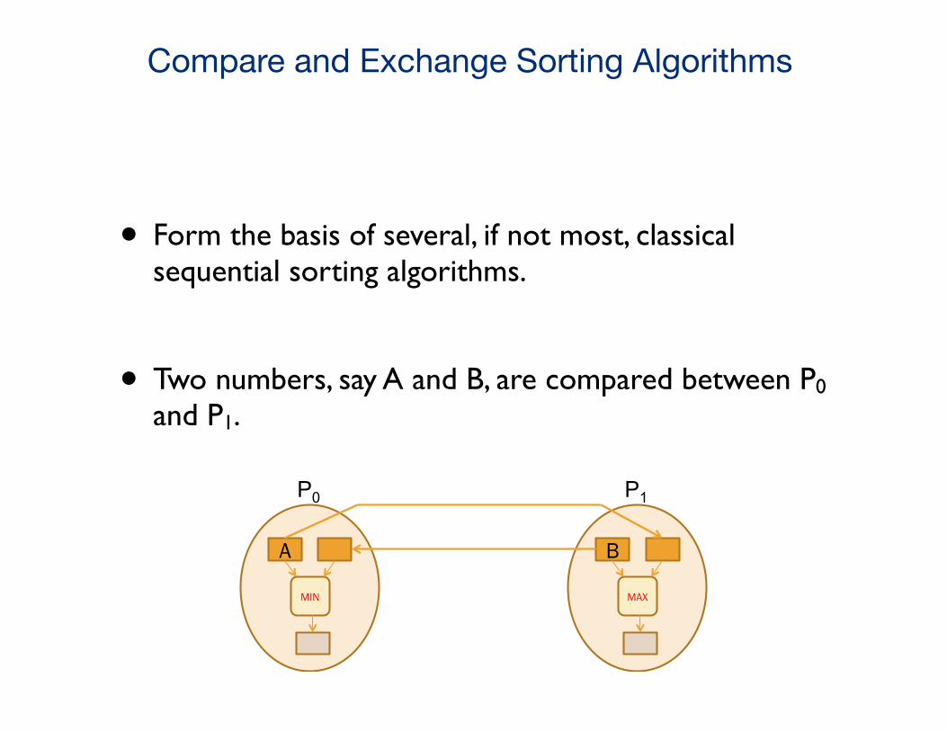
Compare and Exchange Sorting Algorithms

• Form the basis of several, if not most, classical sequential sorting algorithms.

• Two numbers, say A and B, are compared between P0 and P1.

A

MIN

B

MAX

P0 P1

Bubble Sort

• Generic example of a “bad” sorting algorithm.

• Algorithm:

• Compare neighboring elements.

• Swap if neighbor is out of order.

• Two nested loops.

• Stop when a whole pass completes without any swaps.

• Performance:

• Worst: O(n2)

• Average: O(n2)

• Best: O(n)

0 1 2 3 4 5

3 8 0 6 51start:

0 1 2 3 4 5

3 0 6 5 81after pass 1:

0 1 2 3 4 5

0 3 5 6 81after pass 2:

0 1 2 3 4 5

1 3 5 6 80after pass 3:

0 1 2 3 4 5

1 3 5 6 80after pass 4:

fin."The bubble sort seems to have nothing to recommend it, except a catchy name and the fact that it leads to some interesting theoretical problems."

- Donald Knuth, The Art of Computer Programming

Odd-Even Transposition Sort (also Brick Sort)

• Simple sorting algorithm that was introduced in 1972 by Nico Habermann who originally developed it for parallel architectures (“Parallel Neighbor-Sort”).

• A comparison sorting algorithm that is related to bubble sort because it shares a similar approach.

• It compares all (odd-even) indexed pairs of adjacent elements in a list and switches them if they are out of order. The next step repeats this process for (even-odd) indexed pairs and continues alternating until the list is sorted.

• The odd-even transposition sort makes use of a pipelining technique to ultimately run many phases of the bubble sort in parallel.

• The running time of this algorithm is O(n2

)/p ~ O(n)

MergeSort

• Divide and conquer approach

• Characterized by dividing the problem into sub-problems of same form as larger problem. Further divisions into still smaller sub-problems, usually done by recursion.

• Recursive divide-and-conquer amenable to parallelization because separate processes can be used for divided parts. Also usually data is naturally localized.

• Divide the n values to be sorted into two halves

• Recursively sort each half using MergeSort

• Base case n=1 no sorting required

• Merge the two halves (fundamental operation)

• O(n) operation

MergeSort

Div

ide

Conquer

Merge Operation

1 6 5 6 80 0 < 5

0

1 6 5 6 80 1 < 5

0 1

1 6 5 7 80 6 > 5

0 1 5

1 6 5 7 80 6 < 7

0 1 5 6

1 6 5 7 80 6 < 7

0 1 5 6 7 8

fin.

Now, do rest of second array..

O(n) running time because each element is considered (n-1 comparisons)

Parallel MergeSort

• Note: sorting two sub-arrays can be done in parallel. Therefore two recursive calls can be called in parallel.

• The first division phase is essentially scattering the array across the processors.

• The second merge phase can be done in parallel with each processor using a sequential merge operation.

• The overall running time is O(n log n) / (log p) ~ O(n) but the unbalanced processor load and communication makes this algorithm inefficient than expected in practice.

Bitonic MergeSort

• Bitonic Mergesort was introduced by K.E. Batcher in 1968.

• A monotonic sequence is a list that is increasing in value.

• a0, a1, a2, ... an-2, an-1 where a0 < a1 < a2 < ... an-2 < an-1

• A bitonic sequence is defined as a list with two sequences, one increasing and another decreasing; no more than one local minimum and one local maximum. (endpoints (i.e., wraparound) must be considered):

• a0 < a1 < a2 < ... ai-1 < ai > ai+1 ... > an-2 > an-1

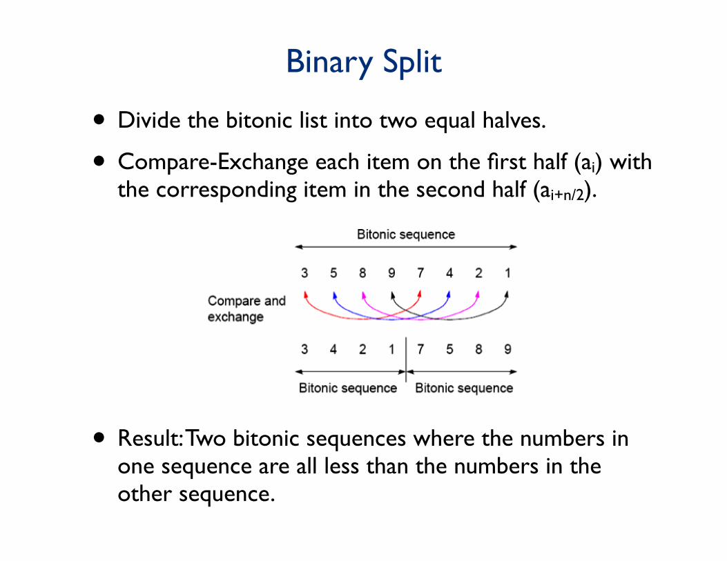
Binary Split

• Divide the bitonic list into two equal halves.

• Compare-Exchange each item on the first half (ai) with the corresponding item in the second half (ai+n/2).

• Result: Two bitonic sequences where the numbers in one sequence are all less than the numbers in the other sequence.

Sorting a Bitonic Sequence via Bitonic Splits

• Compare-and-exchange moves smaller numbers of each pair to left and larger numbers of pair to right.

• Given a bitonic sequence, recursively performing binary splits will sort the list.

• Q: How many binary splits does it takes to sort a list? A: log n

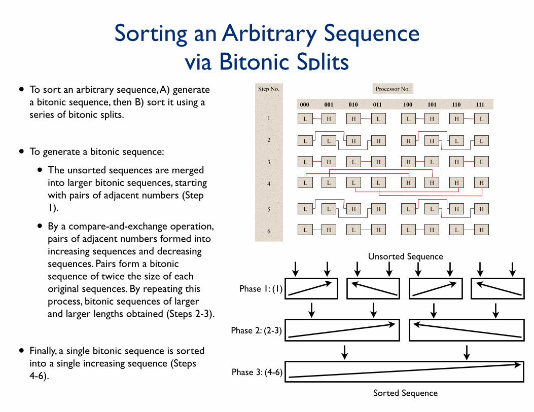
Sorting an Arbitrary Sequence via Bitonic Splits

• To sort an arbitrary sequence, A) generate a bitonic sequence, then B) sort it using a series of bitonic splits.

• To generate a bitonic sequence:

• The unsorted sequences are merged into larger bitonic sequences, starting with pairs of adjacent numbers (Step 1).

• By a compare-and-exchange operation, pairs of adjacent numbers formed into increasing sequences and decreasing sequences. Pairs form a bitonic sequence of twice the size of each original sequences. By repeating this process, bitonic sequences of larger and larger lengths obtained (Steps 2-3).

• Finally, a single bitonic sequence is sorted into a single increasing sequence (Steps 4-6).

Unsorted Sequence

Sorted Sequence

Step No. 1 2 3 4 5 6

Processor No.

000 001 010 011 100 101 110 111

L H H L L H H L

L L H H H H L L

L H L H H L H L

L L L L H H H H

L L H H L L H H

L H L H L H L H

Phase 1: (1)

Phase 2: (2-3)

Phase 3: (4-6)

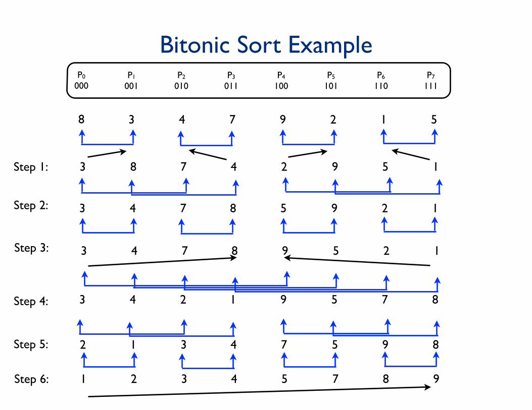
Bitonic Sort ExampleP0

000P1

001P2

010P3

011P4

100P5

101P6

110P7

111

8 3 4 7 9 2 1 5

3 8 7 4 2 9 5 1

3 4 7 8 5 9 2 1

Step 1:

Step 2:

3 4 7 8 9 5 2 1Step 3:

Step 4: 3 4 2 1 9 5 7 8

2 1 3 4 7 5 9 8Step 5:

1 2 3 4 5 7 8 9Step 6:

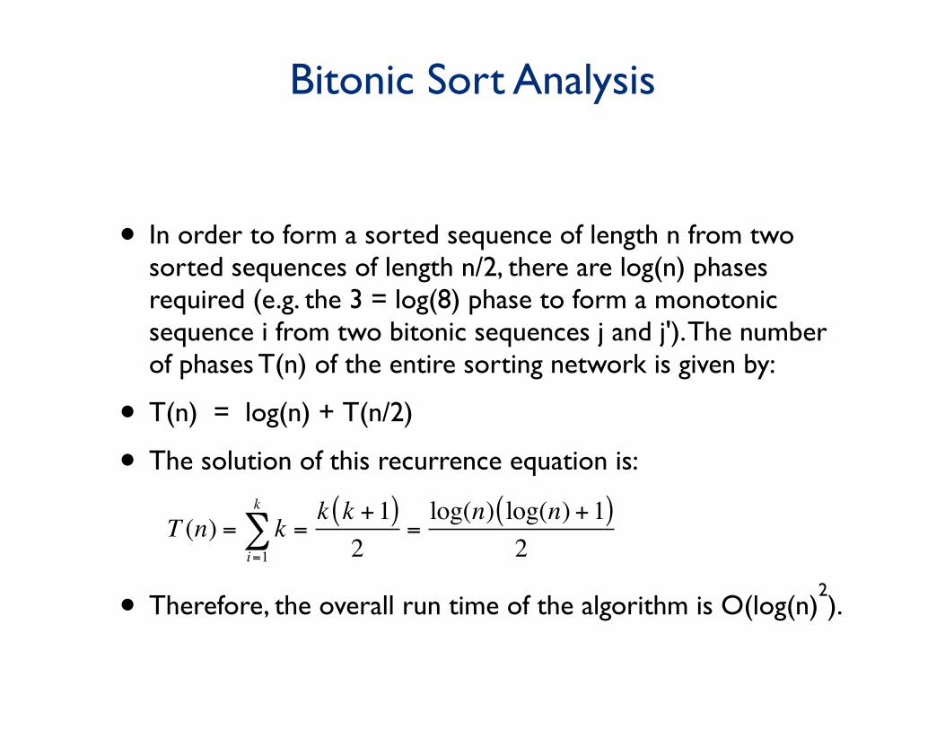
Bitonic Sort Analysis

• In order to form a sorted sequence of length n from two sorted sequences of length n/2, there are log(n) phases required (e.g. the 3 = log(8) phase to form a monotonic sequence i from two bitonic sequences j and j'). The number of phases T(n) of the entire sorting network is given by:

• T(n)  =  log(n) + T(n/2)

• The solution of this recurrence equation is:

• Therefore, the overall run time of the algorithm is O(log(n)2).

T (n) = ki=1

k

∑ =k k +1( )2

=log(n) log(n) +1( )

2

Rank Sort

• Number of elements that are smaller than each selected element is counted. This count provides the position of the selected number, its “rank” in the sorted list.

• First a[0] is read and compared with each of the other numbers, a[1] … a[n-1], recording the number of elements less than a[0].

• Suppose this number is x. This is the index of a[0] in the final sorted list.

• The number a[0] is copied into the final sorted list b[0] … b[n-1], at location b[x]. Actions repeated with the other numbers.

• Overall sequential time complexity of rank sort: T(n)= O(n2

)

// Serial Rank Sort

for (i = 0; i < n; i++) { /* for each number */ x = 0; for (j = 0; j < n; j++) /* count number less than it */ if (a[i] > a[j]) x++; /* copy number into correct place */ b[x] = a[i]; }

// *This code needs to be fixed if // duplicates exist in the sequence.

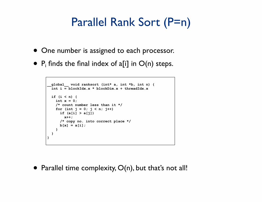
Parallel Rank Sort (P=n)

• One number is assigned to each processor.

• Pi finds the final index of a[i] in O(n) steps.

• Parallel time complexity, O(n), but that’s not all!

__global__ void ranksort (int* a, int *b, int n) { int i = blockIdx.x * blockDim.x + threadIdx.x

if (i < n) { int x = 0; /* count number less than it */ for (int j = 0; j < n; j++) if (a[i] > a[j]) x++; /* copy no. into correct place */ b[x] = a[i]; } } }

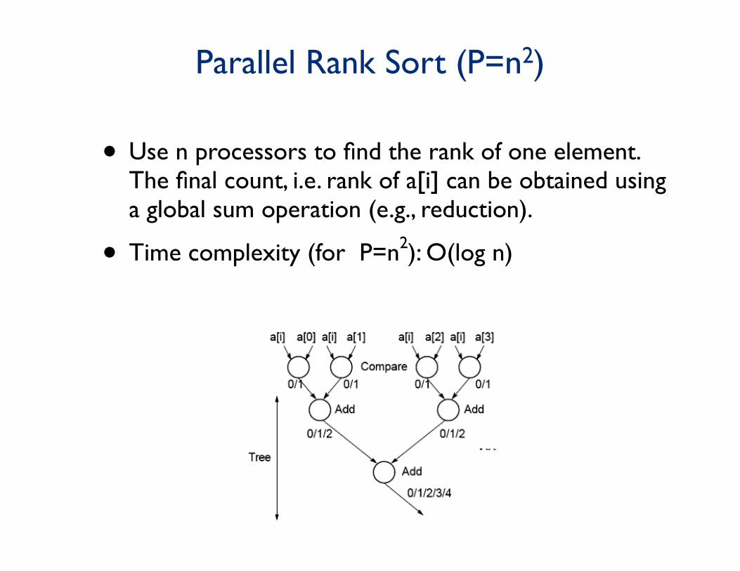
Parallel Rank Sort (P=n2)

• Use n processors to find the rank of one element. The final count, i.e. rank of a[i] can be obtained using a global sum operation (e.g., reduction).

• Time complexity (for P=n2): O(log n)

Bucket Sort

• For an array of N numbers, create M buckets (or bins) for the range of numbers in the array.

• Note in the example that there are two “2”s and two “1”s.

• Each of the elements are put into one of the M buckets.

• This is a stable sorting algorithm.

2 1 3 1 2

1

2

3

Bucket Sort

• For an array of N numbers, create M buckets (or bins) for the range of numbers in the array.

• Note in the example that there are two “2”s and two “1”s.

• Each of the elements are put into one of the M buckets.

• This is a stable sorting algorithm.

2 1 3 1 2

1

2

3

1

2

3

1

2

Bucket Sort

• For an array of N numbers, create M buckets (or bins) for the range of numbers in the array.

• Note in the example that there are two “2”s and two “1”s.

• Each of the elements are put into one of the M buckets.

• This is a stable sorting algorithm.

2 1 3 1 2

1

2

3

1

2

3

1

2

1 1 2 2 3

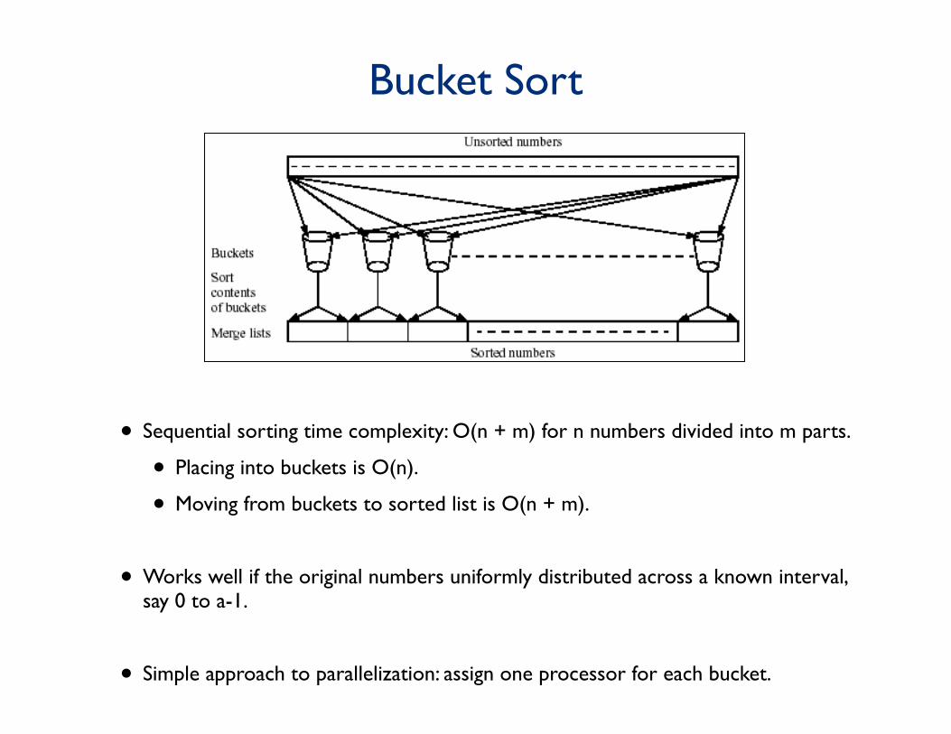
Bucket Sort

• Sequential sorting time complexity: O(n + m) for n numbers divided into m parts.

• Placing into buckets is O(n).

• Moving from buckets to sorted list is O(n + m).

• Works well if the original numbers uniformly distributed across a known interval, say 0 to a-1.

• Simple approach to parallelization: assign one processor for each bucket.

Radix Sort• A radix is the number taken to be the base (or root) of

a system of numbers. For example, for the binary system, the radix is 2, and for the decimal system, the radix is 10.

• Radix Sort is an integer sorting algorithm that uses bucket sort for each digit of an integer (keys) for a sequence of n integers starting from the least significant digit (LSD) to the most significant digit (MSD). The algorithm dates back to a patent in 1887 by Herman Hollerinth on tabulating machines.

• Consider a sequence of n b-bit integers: x = xb-1...x1x0

• For a set of binary numbers, we represent each element as a b-tuple of integers in the range [0,1] and apply radix sort with n=2.

• Serial running time: O(kn2

) where k is the number of digits.

• Parallel running time: O(kn2

)/p ~ O(kn)

Radix Sort Example 1

1001

0010

1101

0001

1110

0010

1110

1001

1101

0001

1001

1101

0001

0010

1110

1001

0001

0010

1101

1110

0001

0010

1001

1101

1110

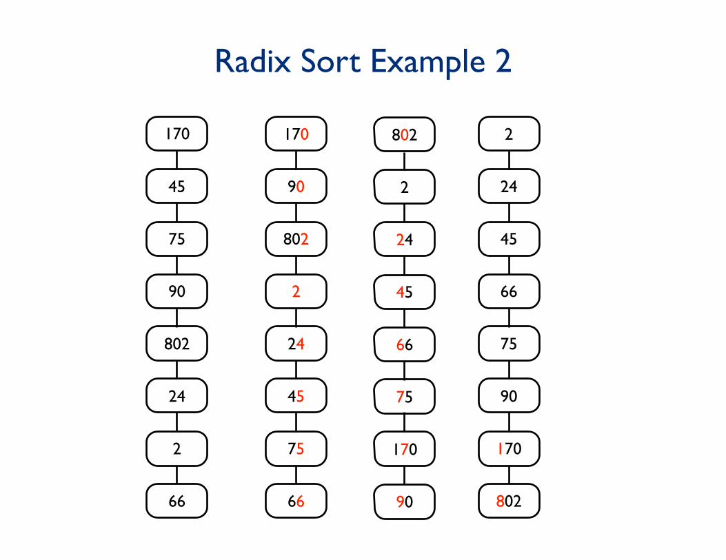
Radix Sort Example 2

170

45

75

90

802

24

2

66

170

90

802

2

24

45

75

66

802

2

24

45

66

75

170

90

2

24

45

66

75

90

170

802

Radix Sort Parallel Implementation

• Two approaches:

• 1) Bucket sort each of the keys.

• 2) Rank sort each of the keys.

Review

• Odd-Even Transposition Sort

• Merge Sort

• Bitonic Sort

• Rank Sort

• Bucket Sort

• Radix Sort