Parallel MATLAB: Single Program Multiple Data · Matlab program that calls a function containing...

Parallel MATLAB:Single Program Multiple Data

John Burkardt (FSU)Gene Cliff (AOE/ICAM - [email protected] )

Justin Krometis (ARC/ICAM - [email protected])James McClure (ARC/ICAM - [email protected])11:00am - 12:00pm, Wednesday, 29 October 2014

.......... NLI ..........FSU: Florida State University

AOE: Department of Aerospace and Ocean EngineeringARC: Advanced Research Computing

ICAM: Interdisciplinary Center for Applied Mathematics

1 / 68

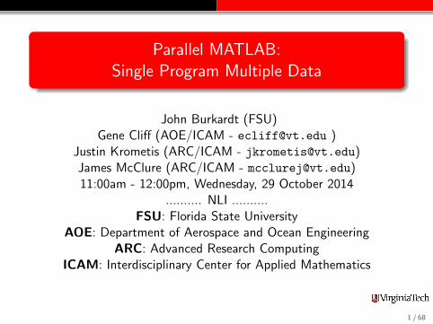
Matlab Parallel Computing

SPMD: Single Program, Multiple Data

QUAD Example

Distributed Arrays

LBVP & FEM 2D HEAT Examples

IMAGE Example

CONTRAST Example

CONTRAST2: Messages

Batch Computing

Conclusion

2 / 68

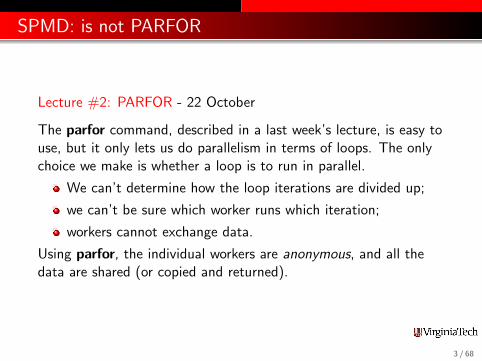
SPMD: is not PARFOR

Lecture #2: PARFOR - 22 October

The parfor command, described in a last week’s lecture, is easy touse, but it only lets us do parallelism in terms of loops. The onlychoice we make is whether a loop is to run in parallel.

We can’t determine how the loop iterations are divided up;

we can’t be sure which worker runs which iteration;

workers cannot exchange data.

Using parfor, the individual workers are anonymous, and all thedata are shared (or copied and returned).

3 / 68

SPMD: is Single Program, Multiple Data

Lecture #3: SPMD - 29 October

The SPMD command (today’s lecture) is like a very simplifiedversion of MPI. There is one client process, supervising workerswho cooperate on a single program. Each worker (sometimes alsocalled a “lab”) has an identifier, knows how many total workersthere are, and can determine its behavior based on that identifier.

each worker runs on a separate core (ideally);

each worker uses separate workspace;

a common program is used;

workers meet at synchronization points;

the client program can examine or modify data on any worker;

any two workers can communicate directly via messages.

4 / 68

SPMD: Getting Workers

An spmd program needs workers to cooperate on the program.

So on a desktop, we issue an interactive matlabpool or parpoolrequest:

pool_obj = parpool(’local’, 4 );results = myfunc ( args );

or use batch to run in the background on your desktop:

job = batch ( ’myscript’, ’Profile’, ’local’, ...’pool’, 4 )

or send the batch command to the Ithaca cluster:

job = batch ( ’myscript’, ’Profile’, ...’ithaca_R2013b’, ’pool’, 7 )

5 / 68

SPMD: The SPMD Environment

Matlab sets up one special agent called the client.

Matlab sets up the requested number of workers, each with acopy of the program. Each worker “knows” it’s a worker, and hasaccess to two special functions:

numlabs(), the number of workers;

labindex(), a unique identifier between 1 and numlabs().

The empty parentheses are usually dropped, but remember, theseare functions, not variables!

If the client calls these functions, they both return the value 1!That’s because when the client is running, the workers are not.The client could determine the number of workers available by

n = matlabpool ( ’size’ ) or n = pool_obj.NumWorkers

6 / 68

SPMD: The SPMD Command

The client and the workers share a single program in which somecommands are delimited within blocks opening with spmd andclosing with end.

The client executes commands up to the first spmd block, when itpauses. The workers execute the code in the block. Once theyfinish, the client resumes execution.

The client and each worker have separate workspaces, but it ispossible for them to communicate and trade information.

The value of variables defined in the “client program” can bereferenced by the workers, but not changed.

Variables defined by the workers can be referenced or changed bythe client, but a special syntax is used to do this.

7 / 68

SPMD: How SPMD Workspaces Are Handled

Client Worker 1 Worker 2a b e | c d f | c d f-------------------------------

a = 3; 3 - - | - - - | - - -b = 4; 3 4 - | - - - | - - -spmd | |c = labindex(); 3 4 - | 1 - - | 2 - -d = c + a; 3 4 - | 1 4 - | 2 5 -

end | |e = a + d{1}; 3 4 7 | 1 4 - | 2 5 -c{2} = 5; 3 4 7 | 1 4 - | 5 6 -spmd | |f = c * b; 3 4 7 | 1 4 4 | 5 6 20

end

8 / 68

SPMD: When is Workspace Preserved?

A program can contain several spmd blocks. When execution ofone block is completed, the workers pause, but they do notdisappear and their workspace remains intact. A variable set in onespmd block will still have that value if another spmd block isencountered. Unless the client has changed it, as in our example.You can imagine the client and workers simply alternate execution.In Matlab, variables defined in a function “disappear” once thefunction is exited. The same thing is true, in the same way, for aMatlab program that calls a function containing spmd blocks.While inside the function, worker data is preserved from one blockto another, but when the function is completed, the worker datadefined there disappears, just as the regular Matlab data does.It’s not legal to nest an smpd block within another spmd block orwithin a parfor loop. Some additional limitations are discussed at

http://www.mathworks.com/help/distcomp/programming-tips_brukbnp-9.html?searchHighlight=nested+spmd

9 / 68



QUAD Example

Distributed Arrays


IMAGE Example

CONTRAST Example

CONTRAST2: Messages

Batch Computing

Conclusion

10 / 68

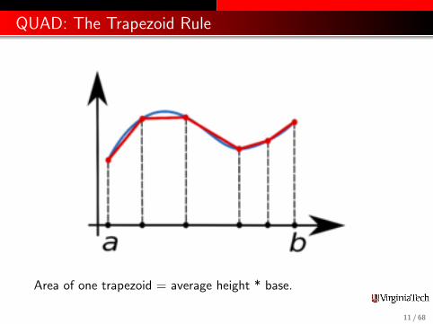
QUAD: The Trapezoid Rule

Area of one trapezoid = average height * base.

11 / 68

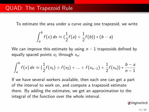
QUAD: The Trapezoid Rule

To estimate the area under a curve using one trapezoid, we write∫ b

af (x) dx ≈ (

1

2f (a) +

1

2f (b)) ∗ (b − a)

We can improve this estimate by using n − 1 trapezoids defined byequally spaced points x1 through xn:∫ b

af (x) dx ≈ (

1

2f (x1) + f (x2) + ... + f (xn−1) +

1

2f (xn)) ∗ b − a

n − 1

If we have several workers available, then each one can get a partof the interval to work on, and compute a trapezoid estimatethere. By adding the estimates, we get an approximation to theintegral of the function over the whole interval.

12 / 68

QUAD: Use the ID to assign work

To simplify things, we’ll assume our original interval is [0,1], andwe’ll let each worker define a and b to mean the ends of itssubinterval. If we have 4 workers, then worker number 3 will beassigned [1

2 , 34 ].

To start our program, each worker figures out its interval:

fprintf ( 1, ’ Set up the integration limits:\n’ );

spmda = ( labindex() - 1 ) / numlabs();b = labindex() / numlabs();

end

13 / 68

QUAD: One Name Must Reference Several Values

Each worker is a program with its own workspace. It can “see” thevariables on the client, but it usually doesn’t know or care what isgoing on on the other workers.

Each worker defines a and b but stores different values there.

The client can “see” the workspace of all the workers. Since thereare multiple values using the same name, the client must specifythe index of the worker whose value it is interested in. Thus a{1}is how the client refers to the variable a on worker 1. The clientcan read or write this value.

Matlab’s name for this kind of variable, indexed using curlybrackets, is a composite variable. The syntax is similar to a cellarray.

The workers can “see” the client’s variables and inherits a copy oftheir values, but cannot change the client’s data.

14 / 68

QUAD: Dealing with Composite Variables

So in QUAD, each worker could print a and b:

spmda = ( labindex() - 1 ) / numlabs();b = labindex() / numlabs();fprintf ( 1, ’ A = %f, B = %f\n’, a, b );

end

———— or the client could print them all ————

spmda = ( labindex() - 1 ) / numlabs();b = labindex() / numlabs();

endfor i = 1 : 4 <-- "numlabs" wouldn’t work here!fprintf ( 1, ’ A = %f, B = %f\n’, a{i}, b{i} );

end

15 / 68

QUAD: The Solution in 4 Parts

Each worker can now carry out its trapezoid computation:

spmdx = linspace ( a, b, n );fx = f ( x ); (Assume f can handle vector input.)quad_part = ( b - a ) / ( n - 1 ) *

* ( 0.5 * fx(1) + sum(fx(2:n-1)) + 0.5 * fx(n) );fprintf ( 1, ’ Partial approx %f\n’, quad_part );

end

with result:

2 Partial approx 0.8746764 Partial approx 0.5675881 Partial approx 0.9799153 Partial approx 0.719414

16 / 68

QUAD: Combining Partial Results

We really want one answer, the sum of all these approximations.

One way to do this is to gather the answers back on the client, andsum them:

quad = sum ( quad_part{1:4} );fprintf ( 1, ’ Approximation %f\n’, quad );

with result:

Approximation 3.14159265

17 / 68

QUAD: Source Code for QUAD FUN

f u n c t i o n v a l u e = quad fun ( n )

%∗∗∗∗∗∗∗∗∗∗∗∗∗∗∗∗∗∗∗∗∗∗∗∗∗∗∗∗∗∗∗∗∗∗∗∗∗∗∗∗∗∗∗∗∗∗∗∗∗∗∗∗∗∗∗∗∗∗∗∗∗∗∗∗∗∗∗∗∗∗∗∗∗∗∗∗∗80%%% QUAD FUN demons t r a t e s MATLAB’ s SPMD command f o r p a r a l l e l programming .%% D i s c u s s i o n :%% A b lock o f s t a t emen t s t ha t beg in w i th the SPMD command a r e c a r r i e d% out i n p a r a l l e l o ve r a l l the LAB’ s . Each LAB has a un ique v a l u e% o f LABINDEX , between 1 and NUMLABS.%% Va lues computed by each LAB are s t o r e d i n a compos i t e v a r i a b l e .% The c l i e n t copy o f MATLAB can a c c e s s t h e s e v a l u e s by u s i n g an i ndex .%% L i c e n s i n g :%% This code i s d i s t r i b u t e d under the GNU LGPL l i c e n s e .%% Mod i f i ed :%% 18 August 2009%% Author :%% John Burkardt%% Parameter s :%% Input , i n t e g e r N, the number o f p o i n t s to use i n each s u b i n t e r v a l .%% Output , r e a l VALUE, the e s t ima t e f o r the i n t e g r a l .%

f p r i n t f ( 1 , ’\n ’ ) ;f p r i n t f ( 1 , ’QUAD FUN\n ’ ) ;f p r i n t f ( 1 , ’ Demonstrate the use o f MATLAB ’ ’ s SPMD command\n ’ ) ;f p r i n t f ( 1 , ’ to c a r r y out a p a r a l l e l computat ion .\n ’ ) ;

%% The e n t i r e i n t e g r a l goes from 0 to 1 .% Each LAB, from 1 to NUMLABS, computes i t s s u b i n t e r v a l [A ,B ] .%

f p r i n t f ( 1 , ’\n ’ ) ;

spmda = ( l a b i n d e x − 1 ) / numlabs ;b = l a b i n d e x / numlabs ;f p r i n t f ( 1 , ’ Lab %d works on [%f ,% f ] .\ n ’ , l a b i nd e x , a , b ) ;

end%% Each LAB now e s t ima t e s the i n t e g r a l , u s i n g N po i n t s .%

f p r i n t f ( 1 , ’\n ’ ) ;

spmdi f ( n == 1 )

q u a d l o c a l = ( b − a ) ∗ f ( ( a + b ) / 2 ) ;e l s e

x = l i n s p a c e ( a , b , n ) ;f x = f ( x ) ;q u a d l o c a l = ( b − a ) ∗ ( f x (1 ) + 2 ∗ sum ( f x ( 2 : n−1) ) + f x ( n ) ) . . .

/ ( 2 . 0 ∗ ( n − 1 ) ) ;endf p r i n t f ( 1 , ’ Lab %d computed app rox imat i on %f\n ’ , l a b i nd e x , q u a d l o c a l ) ;

end%% The v a r i a b l e Q has been computed by each LAB .% Va r i a b l e s computed i n s i d e an SPMD sta tement a r e s t o r e d as ” compos i t e ”% v a r i a b l e s , s i m i l a r to MATLAB’ s c e l l a r r a y s . Out s ide o f an SPMD% statement , compos i t e v a r i a b l e v a l u e s a r e a c c e s s i b l e to the% c l i e n t copy o f MATLAB by i ndex .%% The GPLUS f u n c t i o n adds the i n d i v i d u a l v a l u e s , r e t u r n i n g% the sum to each LAB − so QUAD i s a l s o a compos i t e va lue ,% but a l l i t s v a l u e s a r e equa l .%

spmdquad = gp l u s ( q u a d l o c a l ) ;

end%% Outs ide o f an SPMD statement , the c l i e n t copy o f MATLAB can% ac c e s s any en t r y i n a compos i t e v a r i a b l e by i n d e x i n g i t .%

v a l u e = quad{1} ;

f p r i n t f ( 1 , ’\n ’ ) ;f p r i n t f ( 1 , ’ R e s u l t o f quad ra tu r e c a l c u l a t i o n :\n ’ ) ;f p r i n t f ( 1 , ’ Es t imate QUAD = %24.16 f\n ’ , v a l u e ) ;f p r i n t f ( 1 , ’ Exact v a l u e = %24.16 f\n ’ , p i ) ;f p r i n t f ( 1 , ’ E r r o r = %e\n ’ , abs ( v a l u e − p i ) ) ;f p r i n t f ( 1 , ’\n ’ ) ;f p r i n t f ( 1 , ’QUAD FUN\n ’ ) ;f p r i n t f ( 1 , ’ Normal end o f e x e c u t i o n .\n ’ ) ;

r e t u r nendf un c t i o n v a l u e = f ( x )

%∗∗∗∗∗∗∗∗∗∗∗∗∗∗∗∗∗∗∗∗∗∗∗∗∗∗∗∗∗∗∗∗∗∗∗∗∗∗∗∗∗∗∗∗∗∗∗∗∗∗∗∗∗∗∗∗∗∗∗∗∗∗∗∗∗∗∗∗∗∗∗∗∗∗∗∗∗80%%% F i s the f u n c t i o n to be i n t e g r a t e d .%% D i s c u s s i o n :%% The i n t e g r a l o f F(X) from 0 to 1 i s e x a c t l y PI .%% Mod i f i ed :%% 17 August 2009%% Author :%% John Burkardt%% Parameter s :%% Input , r e a l X(∗ ) , the v a l u e s where the i n t e g r a nd i s to be e v a l u a t e d .%% Output , r e a l VALUE( ) , the i n t e g r a nd v a l u e s .%

v a l u e = 4 .0 . / ( 1 + x .ˆ2 ) ;

r e t u r nend

18 / 68

QUAD: Source Code for QUAD FUN (cont’d)

f p r i n t f ( 1 , ’\n ’ ) ;f p r i n t f ( 1 , ’QUAD FUN\n ’ ) ;f p r i n t f ( 1 , ’ Demonstrate the use o f MATLAB ’ ’ s SPMD command\n ’ ) ;f p r i n t f ( 1 , ’ to c a r r y out a p a r a l l e l computat ion .\n ’ ) ;

%% The e n t i r e i n t e g r a l goes from 0 to 1 .% Each LAB, from 1 to NUMLABS, computes i t s s u b i n t e r v a l [A ,B ] .%

f p r i n t f ( 1 , ’\n ’ ) ;

spmda = ( l a b i n d e x − 1 ) / numlabs ;b = l a b i n d e x / numlabs ;f p r i n t f ( 1 , ’ Lab %d works on [%f ,% f ] .\ n ’ , l a b i nd e x , a , b ) ;

end%% Each LAB now e s t ima t e s the i n t e g r a l , u s i n g N po i n t s .%

f p r i n t f ( 1 , ’\n ’ ) ;

spmdi f ( n == 1 )

q u a d l o c a l = ( b − a ) ∗ f ( ( a + b ) / 2 ) ;e l s e

x = l i n s p a c e ( a , b , n ) ;f x = f ( x ) ;q u a d l o c a l = ( b − a ) ∗ ( f x (1 ) + 2 ∗ sum ( f x ( 2 : n−1) ) + f x ( n ) ) . . .

/ ( 2 . 0 ∗ ( n − 1 ) ) ;endf p r i n t f ( 1 , ’ Lab %d computed app rox imat i on %f\n ’ , l a b i nd e x , q u a d l o c a l ) ;

end19 / 68

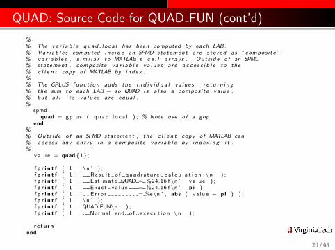
QUAD: Source Code for QUAD FUN (cont’d)

%% The v a r i a b l e q u a d l o c a l has been computed by each LAB .% Va r i a b l e s computed i n s i d e an SPMD sta tement a r e s t o r e d as ” compos i t e ”% v a r i a b l e s , s i m i l a r to MATLAB’ s c e l l a r r a y s . Out s ide o f an SPMD% statement , compos i t e v a r i a b l e v a l u e s a r e a c c e s s i b l e to the% c l i e n t copy o f MATLAB by i ndex .%% The GPLUS f u n c t i o n adds the i n d i v i d u a l v a l u e s , r e t u r n i n g% the sum to each LAB − so QUAD i s a l s o a compos i t e va lue ,% but a l l i t s v a l u e s a r e equa l .%

spmdquad = gp l u s ( q u a d l o c a l ) ; % Note use o f a gop

end%% Outs ide o f an SPMD statement , the c l i e n t copy o f MATLAB can% ac c e s s any en t r y i n a compos i t e v a r i a b l e by i n d e x i n g i t .%

v a l u e = quad{1} ;

f p r i n t f ( 1 , ’\n ’ ) ;f p r i n t f ( 1 , ’ R e s u l t o f quad ra tu r e c a l c u l a t i o n :\n ’ ) ;f p r i n t f ( 1 , ’ Es t imate QUAD = %24.16 f\n ’ , v a l u e ) ;f p r i n t f ( 1 , ’ Exact v a l u e = %24.16 f\n ’ , p i ) ;f p r i n t f ( 1 , ’ E r r o r = %e\n ’ , abs ( v a l u e − p i ) ) ;f p r i n t f ( 1 , ’\n ’ ) ;f p r i n t f ( 1 , ’QUAD FUN\n ’ ) ;f p r i n t f ( 1 , ’ Normal end o f e x e c u t i o n .\n ’ ) ;

r e t u r nend

20 / 68



QUAD Example

Distributed Arrays


IMAGE Example

CONTRAST Example

CONTRAST2: Messages

Batch Computing

Conclusion

21 / 68

DISTRIBUTED: The Client Can Distribute

If the client process has a 300x400 array called a, and there are4 SPMD workers, then the simple command

ad = distributed ( a );

distributes the elements of a by columns:

Worker 1 Worker 2 Worker 3 Worker 4Col: 1:100 | 101:200 | 201:300 | 301:400 ]Row1 [ a b c d | e f g h | i j k l | m n o p ]2 [ A B C D | E F G H | I J K L | M N O P ]

... [ * * * * | * * * * | * * * * | * * * * ]300 [ 1 2 3 4 | 5 6 7 8 | 9 0 1 2 | 3 4 5 6 ]

By default, the last dimension is used for distribution.

22 / 68

DISTRIBUTED: Workers Can Get Their Part

Once the client has distributed the matrix by the command

ad = distributed ( a );

then each worker can make a local variable containing its part:

spmdal = getLocalPart ( ad );[ ml, nl ] = size ( al );

end

On worker 3, [ ml, nl ] = ( 300, 100 ), and al is

[ i j k l ][ I J K L ][ * * * * ][ 9 0 1 2 ]

Notice that local and global column indices will differ!23 / 68

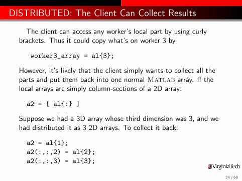
DISTRIBUTED: The Client Can Collect Results

The client can access any worker’s local part by using curlybrackets. Thus it could copy what’s on worker 3 by

worker3_array = al{3};

However, it’s likely that the client simply wants to collect all theparts and put them back into one normal Matlab array. If thelocal arrays are simply column-sections of a 2D array:

a2 = [ al{:} ]

Suppose we had a 3D array whose third dimension was 3, and wehad distributed it as 3 2D arrays. To collect it back:

a2 = al{1};a2(:,:,2) = al{2};a2(:,:,3) = al{3};

24 / 68

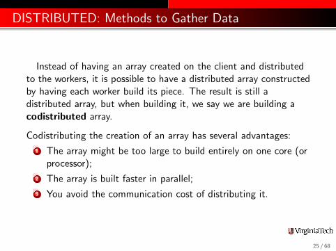
DISTRIBUTED: Methods to Gather Data

Instead of having an array created on the client and distributedto the workers, it is possible to have a distributed array constructedby having each worker build its piece. The result is still adistributed array, but when building it, we say we are building acodistributed array.

Codistributing the creation of an array has several advantages:

1 The array might be too large to build entirely on one core (orprocessor);

2 The array is built faster in parallel;

3 You avoid the communication cost of distributing it.

25 / 68

DISTRIBUTED: Accessing Distributed Arrays

The command al = getLocalPart ( ad ) makes a local copy ofthe part of the distributed array residing on each worker. Althoughthe workers could reference the distributed array directly, the localpart has some uses:

references to a local array are faster;

the worker may only need to operate on the local part; thenit’s easier to write al than to specify ad indexed by theappropriate subranges.

The client can copy a distributed array into a “normal” arraystored entirely in its memory space by the command

a = gather ( ad );

or the client can access and concatenate local parts.

26 / 68

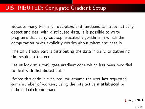
DISTRIBUTED: Conjugate Gradient Setup

Because many Matlab operators and functions can automaticallydetect and deal with distributed data, it is possible to writeprograms that carry out sophisticated algorithms in which thecomputation never explicitly worries about where the data is!

The only tricky part is distributing the data initially, or gatheringthe results at the end.

Let us look at a conjugate gradient code which has been modifiedto deal with distributed data.

Before this code is executed, we assume the user has requestedsome number of workers, using the interactive matlabpool orindirect batch command.

27 / 68

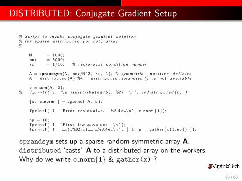
DISTRIBUTED: Conjugate Gradient Setup

% Sc r i p t to i n voke con j uga t e g r a d i e n t s o l u t i o n% f o r s p a r s e d i s t r i b u t e d ( or not ) a r r a y%

N = 1000 ;nnz = 5000 ;r c = 1/10 ; % r e c i p r o c a l c o n d i t i o n number

A = sprandsym (N, nnz/Nˆ2 , rc , 1 ) ; % symmetr ic , p o s i t i v e d e f i n i t eA = d i s t r i b u t e d (A ) ;%A = d i s t r i b u t e d . sprandsym ( ) i s not a v a i l a b l e

b = sum (A, 2 ) ;% f p r i n t f ( 1 , ’\n i s d i s t r i b u t e d ( b ) : %2 i \n ’ , i s d i s t r i b u t e d ( b ) ) ;

[ x , e norm ] = cg emc ( A, b ) ;

f p r i n t f ( 1 , ’ E r r o r r e s i d u a l : %8.4 e \n ’ , e norm {1}) ;

np = 10 ;f p r i n t f ( 1 , ’ F i r s t few x v a l u e s : \n ’ ) ;f p r i n t f ( 1 , ’ x ( %02 i ) = %8.4e \n ’ , [ 1 : np ; ga th e r ( x ( 1 : np ) ) ’ ] ) ;

sprandsym sets up a sparse random symmetric array A.distributed ‘casts’ A to a distributed array on the workers.Why do we write e norm{1} & gather(x) ?

28 / 68

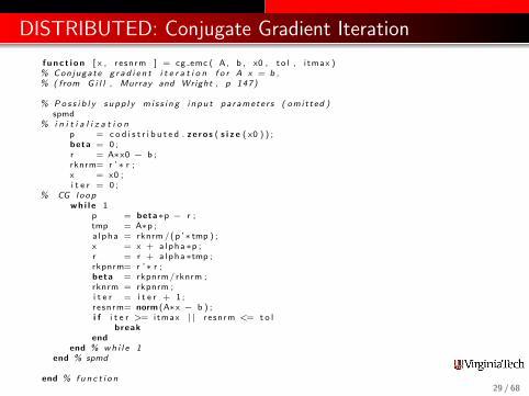
DISTRIBUTED: Conjugate Gradient Iteration

f u n c t i o n [ x , resnrm ] = cg emc ( A, b , x0 , t o l , i tmax )% Conjugate g r a d i e n t i t e r a t i o n f o r A x = b ,% ( from G i l l , Murray and Wright , p 147)

% Po s s i b l y s upp l y m i s s i n g i npu t pa ramete r s ( omi t ted )spmd

% i n i t i a l i z a t i o np = c o d i s t r i b u t e d . ze ro s ( s i z e ( x0 ) ) ;beta = 0 ;r = A∗x0 − b ;rknrm= r ’∗ r ;x = x0 ;i t e r = 0 ;

% CG loopwh i l e 1

p = beta∗p − r ;tmp = A∗p ;a lpha = rknrm /(p ’∗ tmp ) ;x = x + a lpha∗p ;r = r + a lpha∗tmp ;rkpnrm= r ’∗ r ;beta = rkpnrm/ rknrm ;rknrm = rkpnrm ;i t e r = i t e r + 1 ;resnrm= norm (A∗x − b ) ;i f i t e r >= itmax | | resnrm <= t o l

breakend

end % wh i l e 1end % spmd

end % fun c t i o n29 / 68

DISTRIBUTED: Comment

In cg emc.m, we can remove the spmd block and simply invokedistributed(); the operational commands don’t change.

There are several comments worth making:

The communication overhead can be severely increased

Not all Matlab operators have been extended to work withdistributed memory. In particular, (the last time we asked),the backslash or “linear solve” operator x=A\b can’t be usedyet for sparse distributed arrays.

Getting “real” data (as opposed to matrices full of randomnumbers) properly distributed across multiple processorsinvolves more choices and more thought than is suggested bythe conjugate gradient example !

30 / 68



QUAD Example

Distributed Arrays


IMAGE Example

CONTRAST Example

CONTRAST2: Messages

Batch Computing

Conclusion

31 / 68

DISTRIBUTED: Linear Boundary Value Problem

In the next example, we demonstrate a mixed approach whereinthe stiffness matrix (K) is initially constructed as acodistributed array on the workers. Each worker then modifies itslocalPart, and also assembles the local contribution to theforcing term (F). The local forcing arrays are then used to build acodistributed array.

32 / 68

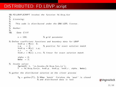
DISTRIBUTED: FD LBVP script

%% FD LBVP SCRIPT i n v o k e s the f u n c t i o n f d l b v p f u n%% L i c e n s i n g :%% This code i s d i s t r i b u t e d under the GNU LGPL l i c e n s e .%% Author :%%% Gene C l i f f

n = 100 ; % g r i d paramete r

% De f i n e c o e f f i c i e n t f u n c t i o n s and boundary data f o r LBVPhnd l p = @( x ) 0 ;c q = 4 ; % p o s i t i v e f o r e xac t s o l u t i o n matchhnd l q = @( x ) c q ;c r = −4;h n d l r = @( x ) c r∗x ; % l i n e a r f o r e xac t s o l u t i o n match

a lpha = 0 ;beta = 2 ;

% Invoke s o l v e rf p r i n t f ( 1 , ’\n Invoke f d l b v p f u n \n ’ ) ;T = f d l b v p f u n (n , hnd l p , hnd l q , hnd l r , a lpha , beta ) ;

% gathe r the d i s t r i b u t e d s o l u t i o n on the c l i e n t p r o c e s s

Tg = ga the r (T) ; % When ’ batch ’ f i n i s h e s the ’ pool ’ i s c l o s e d% and d i s t r i b u t e d data i s l o s t

33 / 68

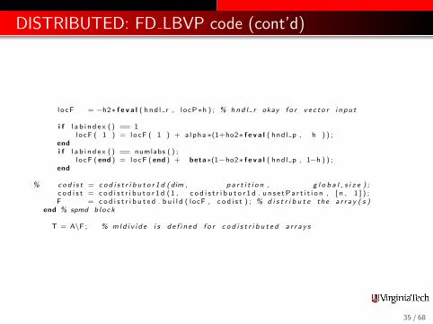
DISTRIBUTED: FD LBVP code

f u n c t i o n T = f d l b v p f u n (n , hnd l p , hnd l q , hnd l r , a lpha , beta )% F i n i t e−d i f f e r e n c e app rox imat i on to the BVP% T’ ’ ( x ) = p ( x ) T’ ( x ) + q ( x ) T( x ) + r ( x ) , 0 \ l e x \ l e 1% with T(0) = alpha , T(1) = beta

% Mod i f i ed :%% 2 March 2012%% Author :%% Gene C l i f f

% We use a un i fo rm g r i d w i th n i n t e r i o r g r i d p o i n t s% From Numer i ca l Ana l y s i s , Burden & Fa i r e s , 2001 , \S˜11 .3

h = 1/(n+1); ho2 = h /2 ; h2 = h∗h ;spmd

A = c o d i s t r i b u t e d . ze ro s (n , n ) ;locP = ge tLo c a lPa r t ( c o d i s t r i b u t e d . co l on (1 , n ) ) ; %index v a l s on l a bl ocP = locP ( : ) ;% make i t a column a r r a y

% Loop ove r columns e n t e r i n g u n i t y above / below the d i a g on a l e n t r y% a long wi th 2 p l u s the a p p r o p r i a t e q f u n c t i o n v a l u e s% Note tha t columns 1 and n a r e e x c e p t i o n s

f o r j j=locP ( 1 ) : locP ( end )% on the d i a g on a lA( j j , j j ) = 2 + h2∗ f e v a l ( hnd l q , j j ∗h ) ;% above the d i a g on a li f j j ˜= 1 ; A( j j −1, j j ) = −1+ho2∗ f e v a l ( hnd l p , ( j j −1)∗h ) ; end% below the d i a g ona li f j j ˜= n ; A( j j +1, j j ) = −1+ho2∗ f e v a l ( hnd l p , j j ∗h ) ; end

end

l o cF = −h2∗ f e v a l ( hnd l r , locP∗h ) ; % hnd l r okay f o r v e c t o r i n pu t

i f l a b i n d e x ( ) == 1locF ( 1 ) = locF ( 1 ) + a lpha∗(1+ho2∗ f e v a l ( hnd l p , h ) ) ;

endi f l a b i n d e x ( ) == numlabs ( ) ;

l o cF ( end ) = locF ( end ) + beta∗(1−ho2∗ f e v a l ( hnd l p , 1−h ) ) ;end

% co d i s t = c o d i s t r i b u t o r 1 d ( dim , p a r t i t i o n , g l o b a l s i z e ) ;c o d i s t = c o d i s t r i b u t o r 1 d (1 , c o d i s t r i b u t o r 1 d . u n s e t P a r t i t i o n , [ n , 1 ] ) ;F = c o d i s t r i b u t e d . b u i l d ( locF , c o d i s t ) ; % d i s t r i b u t e the a r r a y ( s )

end % spmd b lo ck

T = A\F ; % mld i v i d e i s d e f i n e d f o r c o d i s t r i b u t e d a r r a y s

34 / 68

DISTRIBUTED: FD LBVP code (cont’d)

l o cF = −h2∗ f e v a l ( hnd l r , locP∗h ) ; % hnd l r okay f o r v e c t o r i n pu t

i f l a b i n d e x ( ) == 1locF ( 1 ) = locF ( 1 ) + a lpha∗(1+ho2∗ f e v a l ( hnd l p , h ) ) ;

endi f l a b i n d e x ( ) == numlabs ( ) ;

l o cF ( end ) = locF ( end ) + beta∗(1−ho2∗ f e v a l ( hnd l p , 1−h ) ) ;end

% co d i s t = c o d i s t r i b u t o r 1 d ( dim , p a r t i t i o n , g l o b a l s i z e ) ;c o d i s t = c o d i s t r i b u t o r 1 d (1 , c o d i s t r i b u t o r 1 d . u n s e t P a r t i t i o n , [ n , 1 ] ) ;F = c o d i s t r i b u t e d . b u i l d ( locF , c o d i s t ) ; % d i s t r i b u t e the a r r a y ( s )

end % spmd b lo ck

T = A\F ; % mld i v i d e i s d e f i n e d f o r c o d i s t r i b u t e d a r r a y s

35 / 68

DISTRIBUTED: 2D Finite Element Heat Model

Next, we consider an example that combines SPMD anddistributed data to solve a steady state heat equations in 2D, usingthe finite element method. Here we demonstrate a differentstrategy for assembling the required arrays.

Each worker is assigned a subset of the finite element nodes. Thatworker is then responsible for constructing the columns of the(sparse) finite element matrix associated with those nodes.

Although the matrix is assembled in a distributed fashion, it has tobe gathered back into a standard array before the linear systemcan be solved, because sparse linear systems can’t be solved as adistributed array (yet).

This example is available as in the fem 2D heat folder.

36 / 68

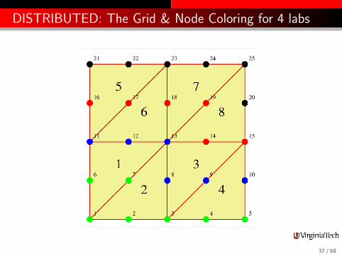
DISTRIBUTED: The Grid & Node Coloring for 4 labs

37 / 68

DISTRIBUTED: Finite Element System matrix

The discretized heat equation results in a linear system of the form

K z = F + b

where K is the stiffness matrix, z is the unknown finite elementcoefficients, F contains source terms and b accounts for boundaryconditions.

In the parallel implementation, the system matrix K and thevectors F and b are distributed arrays. The default distribution ofK by columns essentially associates each SPMD worker with agroup of finite element nodes.

38 / 68

DISTRIBUTED: Finite Element System Matrix

To assemble the matrix, each worker loops over all elements. Ifelement E contains any node associated with the worker, theworker computes the entire local stiffness matrix K . Columns of Kassociated with worker nodes are added to the local part of K. Therest are discarded (which is OK, because they will also becomputed and saved by the worker responsible for those nodes ).

When element 5 is handled, the “blue”, “red” and “black”processors each compute K . But blue only updates column 11 ofK, red columns 16 and 17, and black columns 21, 22, and 23.

At the cost of some redundant computation, we avoid a lot ofcommunication.

39 / 68

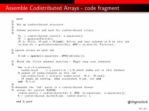
Assemble Codistributed Arrays - code fragment

spmd%% Set up c o d i s t r i b u t e d s t r u c t u r e%% Column p o i n t e r s and such f o r c o d i s t r i b u t e d a r r a y s .%

Vc = c o d i s t r i b u t e d . co l on (1 , n e qu a t i o n s ) ;lP = ge tLo c a lPa r t (Vc ) ;lP 1= lP ( 1 ) ; lP end = lP ( end ) ; %f i r s t and l a s t columns o f K on t h i s l a bc o d i s t V c = g e t C o d i s t r i b u t o r (Vc ) ; dPM = co d i s t V c . P a r t i t i o n ;

. . .% spa r s e a r r a y s on each l a b%

K lab = spa r s e ( n equa t i on s , dPM( l a b i n d e x ) ) ;. . .

% Bu i l d the f i n i t e e l ement ma t r i c e s − Begin l oop ove r e l ement s%

f o r n e l =1: n e l emen t sn o d e s l o c a l = e conn ( n e l , : ) ;% which nodes a r e i n t h i s e l ement

% sub s e t o f nodes / columns on t h i s l a bl a b n o d e s l o c a l = e x t r a c t ( n o d e s l o c a l , lP 1 , lP end ) ;

. . . i f empty do noth ing , e l s e accumulate K lab , e t c endend % n e l

%% Assemble the ’ lab ’ p a r t s i n a c o d i s t r i b u t e d format .% syn tax f o r v e r s i o n R2009b

c o d i s t m a t r i x = c o d i s t r i b u t o r 1 d ( 2 , dPM, [ n equa t i on s , n e qu a t i o n s ] ) ;K = c o d i s t r i b u t e d . b u i l d ( K lab , c o d i s t m a t r i x ) ;

end % spmd

40 / 68

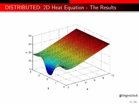
DISTRIBUTED: 2D Heat Equation - The Results

41 / 68



QUAD Example

Distributed Arrays


IMAGE Example

CONTRAST Example

CONTRAST2: Messages

Batch Computing

Conclusion

42 / 68

IMAGE: Image Processing in Parallel

Here is a mysterious SPMD program to be run with 3 workers:

x = imread ( ’ b a l l o o n s . t i f ’ ) ;

y = imno i s e ( x , ’ s a l t & pepper ’ , 0 .30 ) ;

yd = d i s t r i b u t e d ( y ) ;

spmdy l = ge tLo c a lPa r t ( yd ) ;y l = med f i l t 2 ( y l , [ 3 , 3 ] ) ;

end

z ( 1 : 4 80 , 1 : 6 4 0 , 1 ) = y l {1} ;z ( 1 : 4 8 0 , 1 : 6 4 0 , 2 ) = y l {2} ;z ( 1 : 4 8 0 , 1 : 6 4 0 , 3 ) = y l {3} ;

f i g u r e ;subp l o t ( 1 , 3 , 1 ) ; imshow ( x ) ; t i t l e ( ’X ’ ) ;subp l o t ( 1 , 3 , 2 ) ; imshow ( y ) ; t i t l e ( ’Y ’ ) ;subp l o t ( 1 , 3 , 3 ) ; imshow ( z ) ; t i t l e ( ’Z ’ ) ;

Without comments, what can you guess about this program?

43 / 68

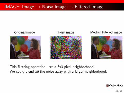
IMAGE: Image → Noisy Image → Filtered Image

This filtering operation uses a 3x3 pixel neighborhood.We could blend all the noise away with a larger neighborhood.

44 / 68

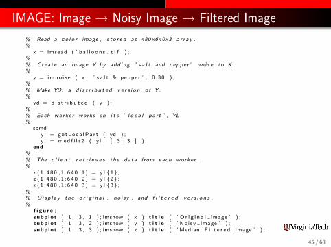
IMAGE: Image → Noisy Image → Filtered Image

% Read a c o l o r image , s t o r e d as 480 x640x3 a r r a y .%

x = imread ( ’ b a l l o o n s . t i f ’ ) ;%% Create an image Y by add ing ” s a l t and pepper ” n o i s e to X .%

y = imno i s e ( x , ’ s a l t & pepper ’ , 0 .30 ) ;%% Make YD, a d i s t r i b u t e d v e r s i o n o f Y .%

yd = d i s t r i b u t e d ( y ) ;%% Each worker works on i t s ” l o c a l p a r t ” , YL .%

spmdy l = ge tLo c a lPa r t ( yd ) ;y l = med f i l t 2 ( y l , [ 3 , 3 ] ) ;

end%% The c l i e n t r e t r i e v e s the data from each worker .%

z ( 1 : 4 80 , 1 : 6 4 0 , 1 ) = y l {1} ;z ( 1 : 4 8 0 , 1 : 6 4 0 , 2 ) = y l {2} ;z ( 1 : 4 8 0 , 1 : 6 4 0 , 3 ) = y l {3} ;

%% Di s p l a y the o r i g i n a l , no i s y , and f i l t e r e d v e r s i o n s .%

f i g u r e ;subp l o t ( 1 , 3 , 1 ) ; imshow ( x ) ; t i t l e ( ’ O r i g i n a l image ’ ) ;subp l o t ( 1 , 3 , 2 ) ; imshow ( y ) ; t i t l e ( ’ No i sy Image ’ ) ;subp l o t ( 1 , 3 , 3 ) ; imshow ( z ) ; t i t l e ( ’ Median F i l t e r e d Image ’ ) ;

45 / 68



QUAD Example

Distributed Arrays


IMAGE Example

CONTRAST Example

CONTRAST2: Messages

Batch Computing

Conclusion

46 / 68

CONTRAST: Image → Contrast Enhancement → Image2

%% Get 4 SPMD worke r s%

mat labpoo l open 4%% Read an image%

x = imageread ( ’ s u r f s u p . t i f ’ ) ;%% Since the image i s b l a c k and white , i t w i l l be d i s t r i b u t e d by columns%

xd = d i s t r i b u t e d ( x ) ;%% Each worker enhances the c o n t r a s t on i t s p o r t i o n o f the p i c t u r e%

spmdx l = ge tLo c a lPa r t ( xd ) ;x l = n l f i l t e r ( x l , [ 3 , 3 ] , @ad j u s tCon t r a s t ) ;x l = u i n t 8 ( x l ) ;

end%% Concatenate the s ubma t r i c e s to as semb le the whole image%

xf spmd = [ x l {:} ] ;

mat l abpoo l c l o s e

47 / 68


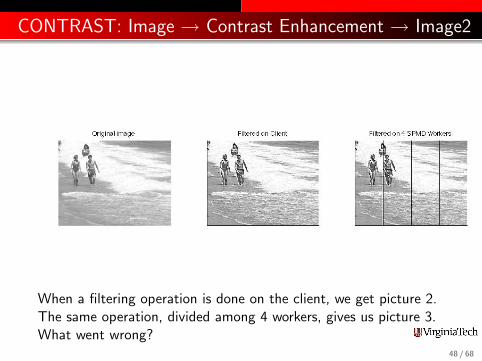
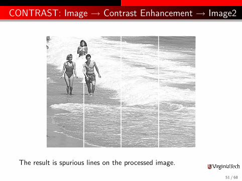
When a filtering operation is done on the client, we get picture 2.The same operation, divided among 4 workers, gives us picture 3.What went wrong?

48 / 68


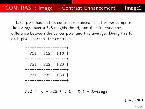
Each pixel has had its contrast enhanced. That is, we computethe average over a 3x3 neighborhood, and then increase thedifference between the center pixel and this average. Doing this foreach pixel sharpens the contrast.

+-----+-----+-----+| P11 | P12 | P13 |+-----+-----+-----+| P21 | P22 | P23 |+-----+-----+-----+| P31 | P32 | P33 |+-----+-----+-----+

P22 <- C * P22 + ( 1 - C ) * Average

49 / 68


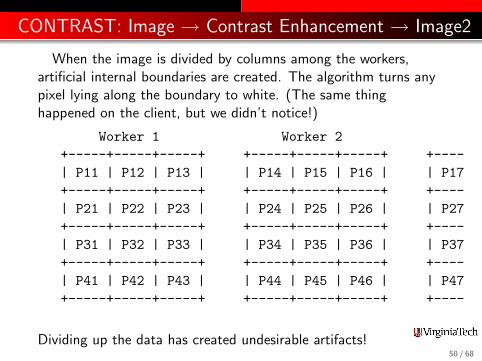
When the image is divided by columns among the workers,artificial internal boundaries are created. The algorithm turns anypixel lying along the boundary to white. (The same thinghappened on the client, but we didn’t notice!)

Worker 1 Worker 2+-----+-----+-----+ +-----+-----+-----+ +----| P11 | P12 | P13 | | P14 | P15 | P16 | | P17+-----+-----+-----+ +-----+-----+-----+ +----| P21 | P22 | P23 | | P24 | P25 | P26 | | P27+-----+-----+-----+ +-----+-----+-----+ +----| P31 | P32 | P33 | | P34 | P35 | P36 | | P37+-----+-----+-----+ +-----+-----+-----+ +----| P41 | P42 | P43 | | P44 | P45 | P46 | | P47+-----+-----+-----+ +-----+-----+-----+ +----

Dividing up the data has created undesirable artifacts!50 / 68


The result is spurious lines on the processed image.

51 / 68



QUAD Example

Distributed Arrays


IMAGE Example

CONTRAST Example

CONTRAST2: Messages

Batch Computing

Conclusion

52 / 68

CONTRAST2: Workers Need to Communicate

The spurious lines would disappear if each worker could just beallowed to peek at the last column of data from the previousworker, and the first column of data from the next worker.

Just as in MPI, Matlab includes commands that allow workers toexchange data.

The command we would like to use is labSendReceive() whichcontrols the simultaneous transmission of data from all the workers.

data_received = labSendReceive ( to, from, data_sent );

53 / 68

CONTRAST2: Whom Do I Want to Communicate With?

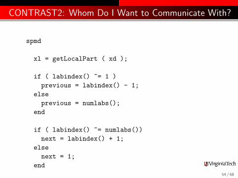
spmd

xl = getLocalPart ( xd );

if ( labindex() ~= 1 )previous = labindex() - 1;

elseprevious = numlabs();

end

if ( labindex() ~= numlabs())next = labindex() + 1;

elsenext = 1;

end54 / 68

CONTRAST2: First Column Left, Last Column Right

column = labSendReceive ( previous, next, xl(:,1) );

if ( labindex() < numlabs() )xl = [ xl, column ];

end

column = labSendReceive ( next, previous, xl(:,end) );

if ( 1 < labindex() )xl = [ column, xl ];

end

55 / 68

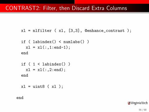
CONTRAST2: Filter, then Discard Extra Columns

xl = nlfilter ( xl, [3,3], @enhance_contrast );

if ( labindex() < numlabs() )xl = xl(:,1:end-1);

end

if ( 1 < labindex() )xl = xl(:,2:end);

end

xl = uint8 ( xl );

end

56 / 68

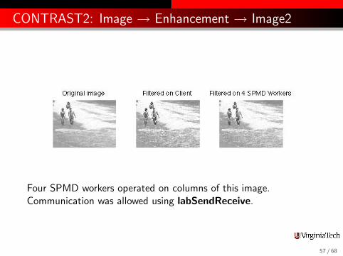
CONTRAST2: Image → Enhancement → Image2

Four SPMD workers operated on columns of this image.Communication was allowed using labSendReceive.

57 / 68



QUAD Example

Distributed Arrays


IMAGE Example

CONTRAST Example

CONTRAST2: Messages

Batch Computing

Conclusion

58 / 68

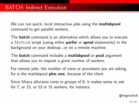
BATCH: Indirect Execution

We can run quick, local interactive jobs using the matlabpoolcommand to get parallel workers.

The batch command is an alternative which allows you to executea Matlab script (using either parfor or spmd statements) in thebackground on your desktop...or on a remote machine.

The batch command includes a matlabpool or pool argumentthat allows you to request a given number of workers.

For remote jobs, the number of cores or processors you are askingfor is the matlabpool plus one, because of the client.

Since Ithaca allocates cores in groups of 8, it makes sense to askfor 7, or 15, or 23 or 31 workers, for instance.

59 / 68

BATCH: Contrast2

Running contrast2 on Ithaca and locally:

% Run on Ithaca

job = batch ( ’contrast2_script’, ...

’Profile’, ’ithaca_R2013b’, ...

’CaptureDiary’, true, ...

’AttachedFiles’, { ’contrast2_fun’, ’contrast_enhance’, ’surfsup.tif’ }, ...

’CurrentDirectory’, ’.’, ...

’pool’, n );

% Run locally

x = imread ( ’surfsup.tif’ );

xf = nlfilter ( x, [3,3], @contrast_enhance );

xf = uint8 ( xf );

% Wait for Ithaca job to complete

wait ( job );

% Load results from Ithaca job

load ( job );

60 / 68

BATCH: Contrast2

Notes:

We need to include both scripts and the input filesurfsup.tif in the AttachedFiles flag

We can do some work before issuing wait()

We leverage two kinds of parallelism:

Parallel (using spmd) on IthacaRun locally while job is running on Ithaca

61 / 68



QUAD Example

Distributed Arrays


IMAGE Example

CONTRAST Example

CONTRAST2: Messages

Batch Computing

Conclusion

62 / 68

CONCLUSION: Summary of Examples

The QUAD example showed a simple problem that could be doneas easily with SPMD as with PARFOR. We just needed to learnabout composite variables!

The CONJUGATE GRADIENT example showed that manyMatlab operations work for distributed arrays, a kind of arraystorage scheme associated with SPMD.

The LBVP & FEM 2D HEAT examples show how to constructlocal arrays and assemble these to codistributed arrays. Thisenables treatment of very large problems.

The IMAGE and CONTRAST examples showed us problems whichcan be broken up into subproblems to be dealt with by SPMDworkers. We also saw that sometimes it is necessary for theseworkers to communicate, using a simple message-passing system.

63 / 68

Conclusion: Desktop-to-Ithaca Submission

If you want to work with parallel Matlab on Ithaca, youmust first get an account, by going to this website:

http://www.arc.vt.edu/forms/account_request.php

For remote submission you must define appropriate Profilefile(s) on your desktop:

http://www.arc.vt.edu/resources/software/matlab/remotesub.php

64 / 68

CONCLUSION: VT MATLAB LISTSERV

There is a local LISTSERV for people interested in Matlab onthe Virginia Tech campus. We try not to post messages hereunless we really consider them of importance!

Important messages include information about workshops, specialMatlab events, and other issues affecting Matlab users.

To subscribe to the mathworks listserver, send email to:

[email protected].

The body of the message should simply be:

subscribe mathworks firstname lastname

65 / 68

CONCLUSION: Where is it?

Matlab Parallel Computing Toolbox Product Documentationhttp://www.mathworks.com/help/toolbox/distcomp/

Gaurav Sharma, Jos Martin,MATLAB: A Language for Parallel Computing,International Journal of Parallel Programming,Volume 37, Number 1, pages 3-36, February 2009.

Links for downloading these Adobe PDF notes, along with azipped-folder containing the Matlab codes can be found onthe ARC Fall 2014 training pagehttp://www.arc.vt.edu/userinfo/training/2014 Fall Matlab NLI.php

66 / 68

AFTERWORD: PMODE

PMODE allows interactive parallel execution ofMatlabcommands. PMODE achieves this by defining and submitting aparallel job, and it opens a Parallel Command Window connectedto the labs running the job. The labs receive commands entered inthe Parallel Command Window, process them, and send thecommand output back to the Parallel Command Window.

pmode start ’local’ 2 will initiate pmode; pmode exit willdelete the parallel job and end the pmode session

This may be a useful way to experiment with computations on thelabs.

67 / 68

THE END

Please complete the evaluation form

Thanks

68 / 68

Parallel MATLAB: Single Program Multiple Data · Matlab program that calls a function containing...

Documents

Transcript of Parallel MATLAB: Single Program Multiple Data · Matlab program that calls a function containing...