Parallel MATLAB at VT - Virginia Tech · At VT, the concurrent ... Setting up intracluster...

Parallel MATLAB at VT

Gene Cliff (AOE/ICAM - [email protected])Justin Krometis (ARC/ICAM - [email protected])

10:00am-1:00pm Tuesday, 27 September 2016.......... NLI ..........

AOE: Department of Aerospace and Ocean EngineeringARC: Advanced Research Computing

ICAM: Interdisciplinary Center for Applied Mathematics

Slide images at: arc.vt.edu/resources/software/matlab

1 / 148

MATLAB Parallel Computing

Introduction

Programming Models

Execution

Example: Quadrature

Conclusion

2 / 148

INTRO: Parallel MATLAB

Parallel MATLAB is an extension of MATLAB that takesadvantage of multicore desktop machines and clusters.

The Parallel Computing Toolbox or PCT runs on a desktop, andcan take advantage of cores (R2014a has no limit, R2013b limit is12, ...). Parallel programs can be run interactively or in batch.

The Matlab Distributed Computing Server (MDCS) controlsparallel execution of MATLAB on a cluster with tens or hundredsof cores.

ARC’s clusters (DragonsTooth, NewRiver, BlueRidge) providesMDCS services for up to 224 cores. Currently, single users arerestricted to 96 cores.

3 / 148

http://www.arc.vt.edu/dragonstooth

http://www.arc.vt.edu/newriver

http://www.arc.vt.edu/blueridge

INTRO: What Do You Need?

1 Your machine should have multiple processors or cores:

On a PC: Start :: Settings :: Control Panel :: SystemOn a Mac: Apple Menu :: About this Mac :: More Info...

2 Your MATLAB must be version 2012a or later:

Go to the HELP menu, and choose About Matlab.

3 You must have the Parallel Computing Toolbox:

At VT, the concurrent (& student) license includes the PCT.The standalone license does not include the PCT.To list all your toolboxes, type the MATLAB command ver.When using an MDCS (server) be sure to use the sameversion of Matlab on your client machine.ARC Clusters currently support R2015a-b, R2016b.

4 / 148


Introduction

Programming Models

Execution

Example: Quadrature

Conclusion

5 / 148

PROGRAMMING: Obtaining Parallelism

Three ways to write a parallel MATLAB program:

suitable for loops can be made into parfor loops;

the spmd statement can define cooperating synchronizedprocessing;

the task feature creates multiple independent programs.

The parfor approach is a limited but simple way to get started.spmd is powerful, but may require rethinking the program/data.The task approach is simple, but suitable only for computationsthat need almost no communication.

6 / 148

PROGRAMMING: PARFOR: Parallel FOR Loops

Lecture #2: PARFOR

The simplest path to parallelism is the parfor statement, whichindicates that a given for loop can be executed in parallel.

When the “client” MATLAB reaches such a loop, the iterations ofthe loop are automatically divided up among the workers, and theresults gathered back onto the client.

Using parfor requires that the iterations are completelyindependent; there are also some restrictions on array-data access.

OpenMP implements a directive for ’parallel for loops’

7 / 148

PROGRAMMING: ”SPMD” Single Program Multiple Data

Lecture #3: SPMD

MATLAB can also work in a simplified kind of MPI model.

There is always a special “client” process.

Each worker process has its own memory and separate ID.

There is a single program, but it is divided into client and workersections; the latter marked by special spmd/end statements.

Workers can “see” the client’s data; the client can access andchange worker data.

The workers can also send messages to other workers.

OpenMP includes constructs similar to spmd.

8 / 148

PROGRAMMING: ”SPMD” Distributed Arrays

SPMD programming includes distributed arrays.

A distributed array is logically one array, and a large set ofMATLAB commands can treat it that way (e.g. ‘backslash’).

However, portions of the array are scattered across multipleprocessors. This means such an array can be really large.

The local part of a distributed array can be operated on by thatprocessor very quickly.

A distributed array can be operated on by explicit commands tothe SPMD workers that “own” pieces of the array, or implicitly bycommands at the global or client level.

9 / 148


Introduction

Programming Models

Execution

Example: Quadrature

Conclusion

10 / 148

EXECUTION: Models

There are several ways to execute a parallel MATLAB program:

Model Command Where It Runs

Interactive matlabpool This machine

Interactiveparpool

(R2013b)This machine

Indirect local batch This machine

Indirect remote batch Remote machine

11 / 148

EXECUTION: Direct using parpool

Parallel MATLAB jobs can be run directly, that is, interactively.

The parpool (previously matlabpool) command is used to reservea given number of workers on the local (or perhaps remote)machine.

Once these workers are available, the user can type commands, runscripts, or evaluate functions, which contain parfor statements.The workers will cooperate in producing results.

Interactive parallel execution is great for desktop debugging ofshort jobs.

Note: Starting in R2013b, if you try to execute a parallel programand a pool of workers is not already open, MATLAB will open itfor you. The pool of workers will then remain open for a time thatcan be specified under Parallel → Parallel Preferences (default =30 minutes).

12 / 148

EXECUTION: Indirect Local using batch

Parallel MATLAB jobs can be run indirectly.

The batch command is used to specify a MATLAB code to beexecuted, to indicate any files that will be needed, and how manyworkers are requested.

The batch command starts the computation in the background.The user can work on other things, and collect the results whenthe job is completed.

The batch command works on the desktop, and can be set up toaccess ARC clusters (e.g. NewRiver).

13 / 148

EXECUTION: Local and Remote MATLAB Workers

14 / 148

EXECUTION: Managing Cluster Profiles

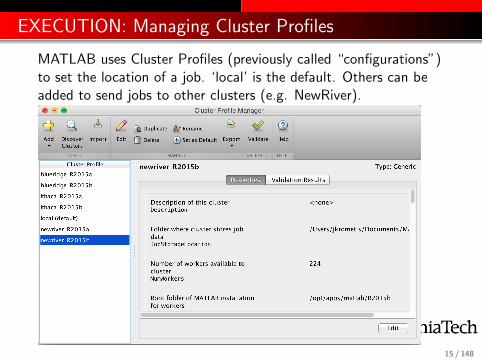
MATLAB uses Cluster Profiles (previously called “configurations”)to set the location of a job. ‘local’ is the default. Others can beadded to send jobs to other clusters (e.g. NewRiver).

15 / 148

EXECUTION: Ways to Run

Interactively, we call parpool and then our function:

mypool = parpool ( ’local’, 4 )

q = quad_fun ( n, a, b );

delete(mypool)

’local’ is a default Cluster Profile defined as part of the PCT.The batch command runs a script, with a Pool argument:

job = batch ( ’quad_script’, ’Pool’, 4 )

(or)

job = batch ( ’Profile’,’local’, ’quad_script’, ...

’Pool’, 4 )

16 / 148

EXECUTION: ARC Clusters

ARC offers resources with Matlab installed, including:

System Usage Nodes Node Description Special Features

DragonsTooth Single-node jobs 48 24 cores, 256GB

(2× Intel Haswell)

NewRiver Data Intensive 126 24 cores, 128 GB 8 K80 GPGPU

(2× Intel Haswell) 16 “big data” nodes

24 512GB nodes

2 3TB nodes

BlueRidge Large-scale CPU, MIC 408 16 cores, 64 GB 260 Intel Xeon Phi

(2× Intel Sandy Bridge) 4 K40 GPU

18 128GB nodes

ARC has a MDCS that can currently accommodate a combinationof jobs with a total of 224 workers. At this time the queueingsoftware imposes a limit of 96 workers per job.

17 / 148

http://www.arc.vt.edu/dragonstooth

http://www.arc.vt.edu/newriver

http://www.arc.vt.edu/blueridge

EXECUTION: Configuring Desktop-to-Cluster Submission

If you want to work with parallel MATLAB on ARC resources,you must first get an account. Go to

http://www.arc.vt.edu/account

Log in (PID and password), select the systems you want towork with and MATLAB in the Software section, and submit.

Steps to set up submission from your desktop include:1 Download and add some files to your MATLAB directory2 Run a script to create a new profile on your desktop.

A new cluster profile (e.g. newriver R2015b) will be createdthat can be used in batch().These steps are described in detail here:

http://www.arc.vt.edu/matlabremote

18 / 148

EXECUTION: Intracluster Submission

You can also submit jobs to ARC clusters from a cluster loginnode.

Pros: Easier to set up. Only one file system to manage.

Cons: Requires logging into the cluster (e.g., with SSH). Haveto use Matlab command line (except on NewRiver).

Setting up intracluster submission is very simple - running aone-question script at the Matlab command line on the ARCcluster.The full steps are described here:

http://www.arc.vt.edu/matlabremote#intracluster

19 / 148

EXECUTION: Job Monitor

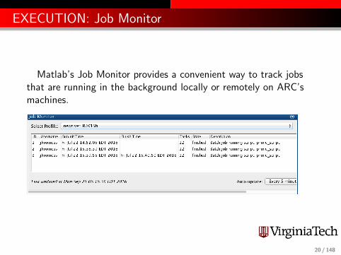
Matlab’s Job Monitor provides a convenient way to track jobsthat are running in the background locally or remotely on ARC’smachines.

20 / 148

MATLAB Parfor

Introduction

Programming Models

Execution

Example: Quadrature

Conclusion

21 / 148

QUAD: Estimating an Integral

22 / 148

QUAD: The QUAD FUN Function

funct ion q = quad fun ( n , a , b )

q =0.0 ;w=(b−a )/ n ;f o r i =1:n

x = ( ( n− i )∗ a+( i −1)∗b ) / ( n−1);f x= 4./(1+ x . ˆ 2 ) ;q = q+w∗ f x ;

end

returnend

23 / 148

QUAD: Comments

The function quad fun estimates the integral of a particularfunction over the interval [a, b].

It does this by evaluating the function at n evenly spaced points,multiplying each value by the weight (b − a)/n.

These quantities can be regarded as the areas of little rectanglesthat lie under the curve, and their sum is an estimate for the totalarea under the curve from a to b.

We could compute these subareas in any order we want.

We could even compute the subareas at the same time, assumingthere is some method to save the partial results and add themtogether in an organized way.

24 / 148

QUAD: The Parallel QUAD FUN Function

funct ion q = quad fun ( n , a , b )

q =0.0 ;w=(b−a )/ n ;

% f o r i =1:n % a v o i d s t a r t i n g p o o lp a r f o r i =1:n

x = ( ( n− i )∗ a+( i −1)∗b ) / ( n−1);f x= 4./(1+ x . ˆ 2 ) ;q = q+w∗ f x ;

end

returnend

25 / 148

QUAD: Comments

The parallel version of quad fun does the same calculations.

The parfor statement changes how this program does thecalculations. It asserts that all the iterations of the loop areindependent, and can be done in any order, or in parallel.

Execution begins with a single processor, the client. When a parforloop is encountered, the client is helped by a “pool” of workers.

Each worker is assigned some iterations of the loop. Once the loopis completed, the client resumes control of the execution.

MATLAB ensures that the results are the same (with exceptions)whether the program is executed sequentially, or with the help ofworkers.

The user can wait until execution time to specify how manyworkers are actually available.

26 / 148

QUAD: Interactive

To run quad fun.m in parallel on your desktop, type:

n = 10000; a = 0.5; b = 1;

pool = parpool(’local’,4)

q = quad_fun ( n, a, b );

delete(pool)

The word local is choosing the local profile, that is, the coresassigned to be workers will be on the local machine.

The value ”4” is the number of workers you are asking for. It canbe up to 12 on a local machine. It does not have to match thenumber of cores you have.

27 / 148

QUAD: Indirect Local BATCH

The batch command, for indirect execution, accepts scripts (andsince R2010b functions). We can make a suitable script calledquad script.m:

n = 10000; a = 0.5; b = 1;

q = quad_fun ( n, a, b )

Now we assemble the job information needed to run the script andsubmit the job:

job = batch ( ’quad_script’, ’Pool’, 4, ...

’Profile’, ’local’, ...

’AttachedFiles’, { ’quad_fun’ } )

28 / 148

QUAD: Indirect Local BATCH

After issuing batch(), the following commands wait for the jobto finish, gather the results, and clear out the job information:

wait ( job ); % no prompt until the job is finished

load ( job ); % load data from the job’s Workspace

delete ( job ); % clean up (destroy prior to R2012a)

Note: You may not want to have Matlab wait for long researchruns. Rather, you may want to submit (perhaps a few times) andcome back and check the results later (e.g., with Job Monitor).

29 / 148

QUAD: Indirect Remote BATCH

The batch command can send your job anywhere, and get theresults back, as long as you have set up an account on the remotemachine, and you have defined a Cluster Profile on your desktopthat tells it how to access the remote machine.

At Virginia Tech, with proper set up, your desktop can send abatch job to an ARC cluster as easily as running locally:

job = batch ( ’quad_script’, ’Pool’, 4, ...

’Profile’, ’newriver_R2015b, ...

’AttachedFiles’, { ’quad_fun’ } )

The job is submitted. You may wait for it, load it anddestroy/delete it, all in the same way as for a local batch job.

30 / 148


Introduction

Programming Models

Execution

Example: Quadrature

Conclusion

31 / 148

CONCLUSION: Summary

Introduction: Parallel Computing Toolbox

Models of parallelism: parfor, spmd, distributed

Models of execution: Interactive vs. Indirect, Local vs.Remote

ARC clusters

Quadrature example: Parallelizing and Running

32 / 148

CONCLUSION: Desktop Experiments

Virginia Tech has a limited number of concurrent MATLABlicenses, and including the Parallel Computing Toolbox.

Since Fall 2011, the PCT is included with the student license.

Run ver in the Matlab Command Window to see what licensesyou have available.

If you don’t have a multicore machine, you won’t see any speedup,but you may still be able to run some ‘parallel’programs.

33 / 148

Matlab Parallel For Loop

Introduction

FMINCON Example

Executing a PARFOR Program

PRIME Example

Classification of variables

ODE SWEEP Example

MD Example

Conclusion

34 / 148

INTRO: Parallel Loops in Matlab

In a previous lecture we discussed Matlab’s Parallel ComputingToolbox (PCT), and the Distributed Computing Server (MDCS)that runs on Virginia Tech’s cluster(s).

As noted previously there are three ways to write a parallelMatlab program:

suitable for loops can be made into parfor loops;

the spmd statement can define cooperating synchronizedprocessing;

the task feature creates multiple independent programs.

Here we focus on parfor loops and on options for parallelism inMatlab provided toolboxes.

35 / 148

INTRO: PARFOR: Parallel FOR Loops

PARFOR

The simplest path to parallelism is the parfor statement, whichindicates that a given for loop can be executed in parallel.

When the “client” Matlab reaches such a loop, the iterations ofthe loop are automatically divided up among the workers, and theresults gathered back onto the client.

Using parfor requires that the iterations are completelyindependent; the results must not depend on the order ofexecution. There are also restrictions on array-data access.

OpenMP implements a directive for ’parallel for loops’

36 / 148

Matlab Parallel Computing

Introduction

FMINCON Example


PRIME Example


ODE SWEEP Example

MD Example

Conclusion

37 / 148

FMINCON: Hidden Parallelism

FMINCON is a popular Matlab function available in theOptimization Toolbox. It finds a local minimizer of a real-valuedfunction of several real variables with constraints:

min F(X) subject to:

A*X <= B,

Aeq*X = Beq (linear constraints)

C(X) <= 0,

Ceq(X) = 0 (nonlinear constraints)

LB <= X <= UB (bounds)

If no derivative (Jacobian) information is supplied by the user, thenFMINCON uses finite differences to estimate these quantities. IfF, C or Ceq are expensive to evaluate, the finite differencing candominate the execution time.

38 / 148

FMINCON: Path of a Boat Against a Current

An example using FMINCON involves a boat trying to cross a riveragainst a current. The boat is given 10 minutes to make thecrossing, and must try to land as far as possible upstream. In thisunusual river, the current is zero midstream, negative above the xaxis, and positive (helpful) below the x axis!

39 / 148

FMINCON: Riding the Helpful Current

The correct solution takes maximum advantage of the favorablecurrent, and then steers back hard to the land on the line y = 1.

40 / 148

FMINCON: Hidden Parallelism

FMINCON uses an options structure that contains defaultsettings. The user can modify these by calling the procedureoptimset. The finite differencing process can be done in parallel ifthe user sets the appropriate option:

options = optimset ( optimset( ’fmincon’ ), ...

’LargeScale’,’off’, ...

’Algorithm’, ’active-set’, ...

’Display’ , ’iter’, ...

’UseParallel’, ’Always’);

[ x_star, f_star, exit ] = fmincon ( h_cost, z0, ...

[], [], [], [], LB, UB, h_cnst, options );

In version 2013a and earlier, the user must invoke thematlabpool command to make workers available!

41 / 148

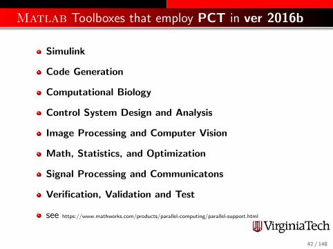
Matlab Toolboxes that employ PCT in ver 2016b

Simulink

Code Generation

Computational Biology

Control System Design and Analysis

Image Processing and Computer Vision

Math, Statistics, and Optimization

Signal Processing and Communicatons

Verification, Validation and Test

see https://www.mathworks.com/products/parallel-computing/parallel-support.html

42 / 148


Introduction

FMINCON Example


PRIME Example


ODE SWEEP Example

MD Example

Conclusion

43 / 148

INTRO: Direct Execution for PARFOR

Parallel MATLAB jobs can be run directly, that is, interactively.

The parpool command is used to reserve a given number ofworkers on the local (or perhaps remote) machine.

Once these workers are available, the user can type commands, runscripts, or evaluate functions, which contain parfor statements.The workers will cooperate in producing results.

Interactive parallel execution is great for desktop debugging ofshort jobs.

It’s an inefficient way to work on a cluster, because no one else canuse the workers until you release them!

So...don’t use the Matlab queue on an ARC Cluster, from yourdesktop machine or from an interactive session on an ARC Clusterlogin node! In our examples, we will indeed use NewRiver, butalways through the indirect batch system.

44 / 148

INTRO: Indirect Execution for PARFOR

Parallel PARFOR Matlab jobs can be run indirectly.

The batch command is used to specify a MATLAB code to beexecuted, to indicate any files that will be needed, and how manyworkers are requested.

The batch command starts the computation in the background.The user can work on other things, and collect the results whenthe job is completed.

The batch command works on the desktop, and can be set up toaccess the an ARC Cluster.

45 / 148

INTRO: batch options

46 / 148


Introduction

FMINCON Example


PRIME Example


ODE SWEEP Example

MD Example

Conclusion

47 / 148

PRIME: The Prime Number Example

For our next example, we want a simple computation involving aloop which we can set up to run for a long time.

We’ll choose a program that determines how many prime numbersthere are between 1 and N.

If we want the program to run longer, we increase the variable N.Doubling N multiplies the run time roughly by 4.

48 / 148

PRIME: The Sieve of Eratosthenes

49 / 148

PRIME: Program Text

f u n c t i o n t o t a l = pr ime ( n )

%% PRIME r e t u r n s the number o f p r imes between 1 and N.

t o t a l = 0 ;

f o r i = 2 : n

pr ime = 1 ;

f o r j = 2 : i − 1i f ( mod ( i , j ) == 0 )

pr ime = 0 ;end

end

t o t a l = t o t a l + pr ime ;

end

r e t u r nend

50 / 148

PRIME: We can run this in parallel

We can parallelize the loop whose index is i, replacing for byparfor. The computations for different values of i are independent.

There is one variable that is not independent of the loops, namelytotal. This is simply computing a running sum (a reductionvariable), and we only care about the final result. Matlab issmart enough to be able to handle this summation in parallel.

To make the program parallel, we replace for by parfor. That’s all!

Beware - reduction assignments require carehttp://www.mathworks.com/help/coder/ug/reduction-assignments-in-parfor-loops.html?searchHighlight=parfor

51 / 148

PRIME: Local Execution With parpool

% m a t l a b p o o l ( ’ open ’ , ’ l o c a l ’ , 4) % o l d form − not s u p p o r t e dR2015ap o o l o b j = p a r p o o l ( ’ l o c a l ’ , 4 ) ; % ( s i n c e R2013b )

n=50;

whi le ( n <= 5000000 )p r i m e s = p r i m e n u m b e r p a r f o r ( n ) ;f p r i n t f ( 1 , ’ %8d %8d\n ’ , n , p r i m e s ) ;n = n ∗ 1 0 ;

end

%m a t l a b p o o l ( ’ c l o s e ’ ) ; not s u p p o r t e d R2015ade lete ( p o o l o b j ) ;

52 / 148

PRIME: Timing

PRIME_PARFOR_RUN

Run PRIME_PARFOR with 0, 2, and 4 labs.

N 1+0 1+2 1+4

50000 0.13 0.10 0.08

500000 3.25 1.66 0.85

5000000 84.9 43.3 21.8

53 / 148

PRIME: Timing Comments

There are many thoughts that come to mind from these results!

This data suggests two conclusions:

Parallelism doesn’t pay until your problem is big enough;

AND

Parallelism doesn’t pay until you have a decent number of workers.

54 / 148


Introduction

FMINCON Example


PRIME Example


ODE SWEEP Example

MD Example

Conclusion

55 / 148

CLASSIFICATION: variable types in PARFOR loopsAdvanced Topics

error if it contains any variables that cannot be uniquely categorized or if anyvariables violate their category restrictions.

Classification Description

Loop Serves as a loop index for arrays

Sliced An array whose segments are operated on by differentiterations of the loop

Broadcast A variable defined before the loop whose value is usedinside the loop, but never assigned inside the loop

Reduction Accumulates a value across iterations of the loop,regardless of iteration order

Temporary Variable created inside the loop, but unlike sliced orreduction variables, not available outside the loop

Each of these variable classifications appears in this code fragment:

��

��

��

��

Loop VariableThe following restriction is required, because changing i in the parfor bodyinvalidates the assumptions MATLAB makes about communication betweenthe client and workers.

2-15

56 / 148

CLASSIFICATION: an example

Advanced Topics

error if it contains any variables that cannot be uniquely categorized or if anyvariables violate their category restrictions.

Classification Description

Loop Serves as a loop index for arrays

Sliced An array whose segments are operated on by differentiterations of the loop

Broadcast A variable defined before the loop whose value is usedinside the loop, but never assigned inside the loop

Reduction Accumulates a value across iterations of the loop,regardless of iteration order

Temporary Variable created inside the loop, but unlike sliced orreduction variables, not available outside the loop

Each of these variable classifications appears in this code fragment:

��

��

��

��

Loop VariableThe following restriction is required, because changing i in the parfor bodyinvalidates the assumptions MATLAB makes about communication betweenthe client and workers.

2-15

NB: ”The range of a parfor statement must be increasingconsecutive integers”Trick Ques: What values to a, i, and d have after exiting the loop ?

57 / 148

Sliced variables:

58 / 148

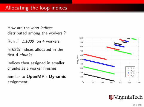
Allocating the loop indices

How are the loop indicesdistributed among the workers ?

Run ii=1:1000 on 4 workers.

≈ 63% indices allocated in thefirst 4 chunks.

Indices then assigned in smallerchunks as a worker finishes

Similar to OpenMP’s Dynamicassignment 0 50 100 150 200 250 300

0

100

200

300

400

500

600

700

800

900

1000

Loop

_ind

ex

W_1W_2W_3W_4

59 / 148

PCT vs Multithread:

At least since R2007a basic Matlab has incorporatedmultithreading

Many linear algebra functions (e.g. LU, QR, SVD) usemultithreads(http://www.mathworks.com/support/solutions/en/data/1-4PG4AN/index.html?solution=1-4PG4AN)

In the PCT each worker/lab runs a single thread

For some codes using parfor will increase the execution time

60 / 148


Introduction

FMINCON Example


PRIME Example


ODE SWEEP Example

MD Example

Conclusion

61 / 148

ODE: A Parameterized Problem

Consider a favorite ordinary differential equation, which describesthe motion of a spring-mass system:

md2x

dt2+ b

dx

dt+ k x = f (t), x(0) = 0, x(0) = v .

62 / 148


Solutions of this equation describe oscillatory behavior; x(t) swingsback and forth, in a pattern determined by the parameters m, b, k ,f and the initial conditions.

Each choice of parameters defines a solution, and let us supposethat the quantity of interest is the maximum deflection xmax thatoccurs for each solution.

We may wish to investigate the influence of b and k on thisquantity, leaving m fixed and f zero.

So our computation might involve creating a plot of xmax(b, k).

63 / 148

ODE: Each Solution has a Maximum Value

64 / 148


Evaluating the implicit function xmax(b, k) requires selecting apair of values for the parameters b and k , solving the ODE over afixed time range, and determining the maximum value of x that isobserved. Each point in our graph will cost us a significant amountof work.

On the other hand, it is clear that each evaluation is completelyindependent, and can be carried out in parallel. Moreover, if weuse a few shortcuts in Matlab, the whole operation becomesquite straightforward!

65 / 148

ODE: The Parallel Code

m = 5 . 0 ;bVa l s = 0 .1 : 0 .05 : 5 ;kVa l s = 1 .5 : 0 .05 : 5 ;

[ bGr id , kGr id ] = meshgr id ( bVals , kVa l s ) ;

peakVa l s = nan ( s i z e ( kGr id ) ) ;

t i c ;

p a r f o r i j = 1 : numel ( kGr id )

[ T, Y ] = ode45 ( @( t , y ) ode sys tem ( t , y , m, bGr id ( i j ) , . . .kGr id ( i j ) ) , [ 0 , 2 5 ] , [ 0 , 1 ] ) ;

peakVa l s ( i j ) = max ( Y( : , 1 ) ) ;

end

toc ;

66 / 148

ODE: PARPOOL or BATCH Execution

pool_obj = parpool(’local’, 4);

ode_sweep_parfor

delete(pool_obj)

ode_sweep_display

- - - - - - - - - - - - - - - - - - - -

job = batch ( ...

’ode_sweep_script’, ...

’Profile’, ’local’, ...

’AttachedFiles’, {’ode_system.m’}, ...

’pool’, 4 );

wait ( job );

load ( job );

ode_sweep_display

delete ( job ) % destroy prior to R2012a

67 / 148

ODE: Display the Results

%% D i s p l a y t he r e s u l t s .%

f i g u r e ;

s u r f ( bVals , kVals , peakVals , ’ EdgeColor ’ , . . .’ I n t e r p ’ , ’ F a c e C o l o r ’ , ’ I n t e r p ’ ) ;

t i t l e ( ’ R e s u l t s o f ODE Parameter Sweep ’ )x l a b e l ( ’ Damping B ’ ) ;y l a b e l ( ’ S t i f f n e s s K ’ ) ;z l a b e l ( ’ Peak D i s p l a c e m e n t ’ ) ;view ( 50 , 30 )

68 / 148


69 / 148

ODE: A Very Loosely Coupled Calculation

In the PRIME program, the parfor loop was invoked in the outerloop; in each iteration there is a reasonable workload/.

In the ODE parameter sweep, we have several thousand IVP’s tosolve, but we could solve them in any order, on various computers,or any way we wanted to. All that was important was that whenthe computations were completed, every value xmax(b, x) hadbeen computed.

This kind of loosely-coupled problem can be treated as a taskcomputing problem, wherein Matlab can treat this problem as acollection of many little tasks to be computed in an arbitraryfashion and assembled at the end.

70 / 148


Introduction

FMINCON Example


PRIME Example


ODE SWEEP Example

MD Example

Conclusion

71 / 148

MD: A Molecular Dynamics Simulation

Compute the positions and velocities of N particles at a sequenceof times. The particles exert a weak attractive force on each other.

72 / 148

MD: The Molecular Dynamics Example

The MD program runs a simple molecular dynamics simulation.

There are N molecules being simulated.

The program runs a long time; a parallel version would run faster.

There are many for loops in the program that we might replace byparfor, but it is a mistake to try to parallelize everything!

Matlab has a profile command that can report where the CPUtime was spent - which is where we should try to parallelize.

73 / 148

MD: Profile the Sequential Code

>> profile on

>> md

>> profile viewer

Step Potential Kinetic (P+K-E0)/E0

Energy Energy Energy Error

1 498108.113974 0.000000 0.000000e+00

2 498108.113974 0.000009 1.794265e-11

... ... ... ...

9 498108.111972 0.002011 1.794078e-11

10 498108.111400 0.002583 1.793996e-11

CPU time = 415.740000 seconds.

Wall time = 378.828021 seconds.

74 / 148

MD: Where is Execution Time Spent?This is a static copy of a profile report

Home

Profile SummaryGenerated 27-Apr-2009 15:37:30 using cpu time.

Function Name Calls Total Time Self Time* Total Time Plot

(dark band = self time)

md 1 415.847 s 0.096 s

compute 11 415.459 s 410.703 s

repmat 11000 4.755 s 4.755 s

timestamp 2 0.267 s 0.108 s

datestr 2 0.130 s 0.040 s

timefun/private/formatdate 2 0.084 s 0.084 s

update 10 0.019 s 0.019 s

datevec 2 0.017 s 0.017 s

now 2 0.013 s 0.001 s

datenum 4 0.012 s 0.012 s

datestr>getdateform 2 0.005 s 0.005 s

initialize 1 0.005 s 0.005 s

etime 2 0.002 s 0.002 s

Self time is the time spent in a function excluding the time spent in its child functions. Self time also includes overhead resulting from

the process of profiling.

Profile Summary file://localhost/Users/burkardt/public_html/m_src/md/md_profile.txt/file0.html

1 of 1 4/27/09 3:39 PM

75 / 148

MD: The COMPUTE Function

f u n c t i o n [ f , pot , k i n ] = compute ( np , nd , pos , v e l , mass )

f = z e r o s ( nd , np ) ;pot = 0 . 0 ;

f o r i = 1 : npf o r j = 1 : np

i f ( i ˜= j )r i j ( 1 : nd ) = pos ( 1 : nd , i ) − pos ( 1 : nd , j ) ;d = s q r t ( sum ( r i j ( 1 : nd ) . ˆ 2 ) ) ;d2 = min ( d , p i / 2 .0 ) ;pot = pot + 0 .5 ∗ s i n ( d2 ) ∗ s i n ( d2 ) ;f ( 1 : nd , i ) = f ( 1 : nd , i ) − r i j ( 1 : nd ) ∗ s i n ( 2 . 0 ∗ d2 ) / d ;

endend

end

k i n = 0 .5 ∗ mass ∗ sum ( v e l ( 1 : nd , 1 : np ) . ˆ 2 ) ;

r e t u r nend

76 / 148

MD: Can We Use PARFOR?

The compute function fills the force vector f(i) using a for loop.

Iteration i computes the force on particle i, determining thedistance to each particle j, squaring, truncating, taking the sine.

The computation for each particle is “independent”; nothingcomputed in one iteration is needed by, nor affects, thecomputation in another iteration. We could compute each value ona separate worker, at the same time.

The Matlab command parfor will distribute the iterations of thisloop across the available workers.

Tricky question: Could we parallelize the j loop instead?

Tricky question: Could we parallelize both loops?

77 / 148

MD: Speedup

Replacing “for i” by “parfor i”, here is our speedup:

78 / 148

MD: Speedup

Parallel execution gives a huge improvement in this example.

There is some overhead in starting up the parallel process, and intransferring data to and from the workers each time a parfor loopis encountered. So we should not simply try to replace every forloop with parfor.

That’s why we first searched for the function that was using mostof the execution time.

The parfor command is the simplest way to make a parallelprogram, but in the next lecture we will see some alternatives.

79 / 148

MD: PARFOR is Particular

We were only able to parallelize the loop because the iterationswere independent, that is, the results did not depend on the orderin which the iterations were carried out.

In fact, to use Matlab’ parfor in this case requires some extraconditions, which are discussed in the PCT User’s Guide. Briefly,parfor is usable when vectors and arrays that are modified in thecalculation can be divided up into distinct slices, so that each sliceis only needed for one iteration.

This is a stronger requirement than independence of order!

Trick question: Why was the scalar value POT acceptable?

80 / 148


Introduction

FMINCON Example


PRIME Example


ODE SWEEP Example

MD Example

Conclusion

81 / 148

CONCLUSION: Summary of Examples

In the FMINCON example, all we had to do to take advantage ofparallelism was set an option (and possibly make sure someworkers were available).

By timing the PRIME example, we saw that it is inefficient to workon small problems, or with only a few processors.

In the ODE SWEEP example, the loop we modified was not asmall internal loop, but a big “outer” loop that defined the wholecalculation.

In the MD example, we did a profile first to identify where thework was.

82 / 148


We only briefly mentioned the limitations of the parfor statement.

You can look in the User’s Guide for some more information onwhen you are allowed to turn a for loop into a parfor loop. It’s notas simple as just knowing that the loop iterations are independent.Matlab has concerns about data usage as well.

Matlabs built in program editor (mlint) knows all about therules for using parfor. You can experiment by changing a for toparfor, and the editor will immediately complain to you if there is areason that Matlab will not accept a parfor version of the loop.

83 / 148

Matlab Parallel Computing; SPMD

SPMD: Single Program, Multiple Data

QUAD Example

Distributed Arrays

LBVP & FEM 2D HEAT Examples

IMAGE Example

CONTRAST Example

CONTRAST2: Messages

Batch Computing

Conclusion

84 / 148

SPMD: is not PARFOR

Previous Lecture: PARFOR

The parfor command, described earlier, is easy to use, but it onlylets us do parallelism in terms of loops. The only choice we makeis whether a loop is to run in parallel.

We can’t determine how the loop iterations are divided up;

we can’t be sure which worker runs which iteration;

workers cannot exchange data.

Using parfor, the individual workers are anonymous, and all thedata are shared (or copied and returned).

85 / 148

SPMD: is Single Program, Multiple Data

Lecture: SPMD

The SPMD construct is like a very simplified version of MPI.There is one client process, supervising workers who cooperate ona single program. Each worker (sometimes also called a “lab”) hasan identifier, knows how many total workers there are, and candetermine its behavior based on that identifier.

each worker runs on a separate core (ideally);

each worker uses a separate workspace;

a common program is used;

workers meet at synchronization points;

the client program can examine or modify data on any worker;

any two workers can communicate directly via messages.

86 / 148

SPMD: The SPMD Environment

Matlab sets up one special agent called the client.

Matlab sets up the requested number of workers, each with acopy of the program. Each worker “knows” it’s a worker, and hasaccess to two special functions:

numlabs(), the number of workers;

labindex(), a unique identifier between 1 and numlabs().

The empty parentheses are usually dropped, but remember, theseare functions, not variables!

If the client calls these functions, they both return the value 1!That’s because when the client is running, the workers are not.The client could determine the number of workers available by

n = matlabpool ( ’size’ ) or

n = pool_obj.NumWorkers

87 / 148

SPMD: The SPMD Command

The client and the workers share a single program in which somecommands are delimited within blocks opening with spmd andclosing with end.

The client executes commands up to the first spmd block, when itpauses. The workers execute the code in the block. Once theyfinish, the client resumes execution.

The client and each worker have separate workspaces, but it ispossible for them to communicate and trade information.

The value of variables defined in the “client program” can bereferenced by the workers, but not changed.

Variables defined by the workers can be referenced or changed bythe client, but a special syntax is used to do this.

88 / 148

SPMD: How SPMD Workspaces Are Handled

Client Worker 1 Worker 2

a b e | c d f | c d f

-------------------------------

a = 3; 3 - - | - - - | - - -

b = 4; 3 4 - | - - - | - - -

spmd | |

c = labindex(); 3 4 - | 1 - - | 2 - -

d = c + a; 3 4 - | 1 4 - | 2 5 -

end | |

e = a + d{1}; 3 4 7 | 1 4 - | 2 5 -

c{2} = 5; 3 4 7 | 1 4 - | 5 6 -

spmd | |

f = c * b; 3 4 7 | 1 4 4 | 5 6 20

end

89 / 148

SPMD: When is Workspace Preserved?

A program can contain several spmd blocks. When execution ofone block is completed, the workers pause, but they do notdisappear and their workspace remains intact. A variable set in onespmd block will still have that value if another spmd block isencountered. Unless the client has changed it, as in our example.You can imagine the client and workers simply alternate execution.In Matlab, variables defined in a function “disappear” once thefunction is exited. The same thing is true, in the same way, for aMatlab program that calls a function containing spmd blocks.While inside the function, worker data is preserved from one blockto another, but when the function is completed, the worker datadefined there disappears, just as the regular Matlab data does.It’s not legal to nest an smpd block within another spmd block orwithin a parfor loop. Some additional limitations are discussed at

http://www.mathworks.com/help/distcomp/programming-tips_brukbnp-9.html?searchHighlight=nested+spmd

90 / 148



QUAD Example

Distributed Arrays


IMAGE Example

CONTRAST Example

CONTRAST2: Messages

Batch Computing

Conclusion

91 / 148

QUAD: The Trapezoid Rule

Area of one trapezoid = average height * base.

92 / 148

QUAD: The Trapezoid Rule

To estimate the area under a curve using one trapezoid, we write∫ b

af (x) dx ≈ (

1

2f (a) +

1

2f (b)) ∗ (b − a)

We can improve this estimate by using n − 1 trapezoids defined byequally spaced points x1 through xn:∫ b

af (x) dx ≈ (

1

2f (x1) + f (x2) + ... + f (xn−1) +

1

2f (xn)) ∗ b − a

n − 1

If we have several workers available, then each one can get a partof the interval to work on, and compute a trapezoid estimatethere. By adding the estimates, we get an approximation to theintegral of the function over the whole interval.

93 / 148

QUAD: Use the ID to assign work

To simplify things, we’ll assume our original interval is [0,1], andwe’ll let each worker define a and b to mean the ends of itssubinterval. If we have 4 workers, then worker number 3 will beassigned [12 ,

34 ].

To start our program, each worker figures out its interval:

fprintf ( 1, ’ Set up the integration limits:\n’ );

spmd

a = ( labindex() - 1 ) / numlabs();

b = labindex() / numlabs();

end

94 / 148

QUAD: One Name Must Reference Several Values

Each worker has its own workspace. It can “see” the variables onthe client, but it usually doesn’t know or care what is going on onthe other workers.

Each worker defines a and b but stores different values there.

The client can “see” the workspace of all the workers. Since thereare multiple values using the same name, the client must specifythe index of the worker whose value it is interested in. Thus a{1}is how the client refers to the variable a on worker 1. The clientcan read or write this value.

Matlab’s name for this kind of variable, indexed using curlybrackets, is a composite variable. The syntax is similar to a cellarray.

The workers can “see” the client’s variables and inherits a copy oftheir values, but cannot change the client’s data.

95 / 148

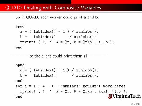
QUAD: Dealing with Composite Variables

So in QUAD, each worker could print a and b:

spmd



fprintf ( 1, ’ A = %f, B = %f\n’, a, b );

end

———— or the client could print them all ————

spmd



end

for i = 1 : 4 <-- "numlabs" wouldn’t work here!

fprintf ( 1, ’ A = %f, B = %f\n’, a{i}, b{i} );

end

96 / 148

QUAD: The Solution in 4 Parts

Each worker can now carry out its trapezoid computation:

spmd

x = linspace ( a, b, n );

fx = f ( x ); (Assume f can handle vector input.)

quad_part = ( b - a ) / ( n - 1 ) *

* ( 0.5 * fx(1) + sum(fx(2:n-1)) + 0.5 * fx(n) );

fprintf ( 1, ’ Partial approx %f\n’, quad_part );

end

with result:

2 Partial approx 0.874676




97 / 148

QUAD: Combining Partial Results

We really want one answer, the sum of all these approximations.

One way to do this is to gather the answers back on the client, andsum them:

quad = sum ( quad_part{1:4} );

fprintf ( 1, ’ Approximation %f\n’, quad );

with result:

Approximation 3.14159265

98 / 148

QUAD: Source Code for QUAD FUN

f u n c t i o n v a l u e = quad fun ( n )

%∗∗∗∗∗∗∗∗∗∗∗∗∗∗∗∗∗∗∗∗∗∗∗∗∗∗∗∗∗∗∗∗∗∗∗∗∗∗∗∗∗∗∗∗∗∗∗∗∗∗∗∗∗∗∗∗∗∗∗∗∗∗∗∗∗∗∗∗∗∗∗∗∗∗∗∗∗80%%% QUAD FUN demons t r a t e s MATLAB’ s SPMD command f o r p a r a l l e l programming .%% D i s c u s s i o n :%% A b lock o f s t a t emen t s t ha t beg in w i th the SPMD command a r e c a r r i e d% out i n p a r a l l e l o ve r a l l the LAB’ s . Each LAB has a un ique v a l u e% o f LABINDEX , between 1 and NUMLABS.%% Va lues computed by each LAB are s t o r e d i n a compos i t e v a r i a b l e .% The c l i e n t copy o f MATLAB can a c c e s s t h e s e v a l u e s by u s i n g an i ndex .%% L i c e n s i n g :%% This code i s d i s t r i b u t e d under the GNU LGPL l i c e n s e .%% Mod i f i ed :%% 18 August 2009%% Author :%% John Burkardt%% Parameter s :%% Input , i n t e g e r N, the number o f p o i n t s to use i n each s u b i n t e r v a l .%% Output , r e a l VALUE, the e s t ima t e f o r the i n t e g r a l .%

f p r i n t f ( 1 , ’\n ’ ) ;f p r i n t f ( 1 , ’QUAD FUN\n ’ ) ;f p r i n t f ( 1 , ’ Demonstrate the use o f MATLAB ’ ’ s SPMD command\n ’ ) ;f p r i n t f ( 1 , ’ to c a r r y out a p a r a l l e l computat ion .\n ’ ) ;

%% The e n t i r e i n t e g r a l goes from 0 to 1 .% Each LAB, from 1 to NUMLABS, computes i t s s u b i n t e r v a l [A ,B ] .%

f p r i n t f ( 1 , ’\n ’ ) ;

spmda = ( l a b i n d e x − 1 ) / numlabs ;b = l a b i n d e x / numlabs ;f p r i n t f ( 1 , ’ Lab %d works on [%f ,% f ] .\ n ’ , l a b i nd e x , a , b ) ;

end%% Each LAB now e s t ima t e s the i n t e g r a l , u s i n g N po i n t s .%

f p r i n t f ( 1 , ’\n ’ ) ;

spmdi f ( n == 1 )

q u a d l o c a l = ( b − a ) ∗ f ( ( a + b ) / 2 ) ;e l s e

x = l i n s p a c e ( a , b , n ) ;f x = f ( x ) ;q u a d l o c a l = ( b − a ) ∗ ( f x (1 ) + 2 ∗ sum ( f x ( 2 : n−1) ) + f x ( n ) ) . . .

/ ( 2 . 0 ∗ ( n − 1 ) ) ;endf p r i n t f ( 1 , ’ Lab %d computed app rox imat i on %f\n ’ , l a b i nd e x , q u a d l o c a l ) ;

end%% The v a r i a b l e Q has been computed by each LAB .% Va r i a b l e s computed i n s i d e an SPMD sta tement a r e s t o r e d as ” compos i t e ”% v a r i a b l e s , s i m i l a r to MATLAB’ s c e l l a r r a y s . Out s ide o f an SPMD% statement , compos i t e v a r i a b l e v a l u e s a r e a c c e s s i b l e to the% c l i e n t copy o f MATLAB by i ndex .%% The GPLUS f u n c t i o n adds the i n d i v i d u a l v a l u e s , r e t u r n i n g% the sum to each LAB − so QUAD i s a l s o a compos i t e va lue ,% but a l l i t s v a l u e s a r e equa l .%

spmdquad = gp l u s ( q u a d l o c a l ) ;

end%% Outs ide o f an SPMD statement , the c l i e n t copy o f MATLAB can% ac c e s s any en t r y i n a compos i t e v a r i a b l e by i n d e x i n g i t .%

v a l u e = quad{1} ;

f p r i n t f ( 1 , ’\n ’ ) ;f p r i n t f ( 1 , ’ R e s u l t o f quad ra tu r e c a l c u l a t i o n :\n ’ ) ;f p r i n t f ( 1 , ’ Es t imate QUAD = %24.16 f\n ’ , v a l u e ) ;f p r i n t f ( 1 , ’ Exact v a l u e = %24.16 f\n ’ , p i ) ;f p r i n t f ( 1 , ’ E r r o r = %e\n ’ , abs ( v a l u e − p i ) ) ;f p r i n t f ( 1 , ’\n ’ ) ;f p r i n t f ( 1 , ’QUAD FUN\n ’ ) ;f p r i n t f ( 1 , ’ Normal end o f e x e c u t i o n .\n ’ ) ;

r e t u r nendf u n c t i o n v a l u e = f ( x )

%∗∗∗∗∗∗∗∗∗∗∗∗∗∗∗∗∗∗∗∗∗∗∗∗∗∗∗∗∗∗∗∗∗∗∗∗∗∗∗∗∗∗∗∗∗∗∗∗∗∗∗∗∗∗∗∗∗∗∗∗∗∗∗∗∗∗∗∗∗∗∗∗∗∗∗∗∗80%%% F i s the f u n c t i o n to be i n t e g r a t e d .%% D i s c u s s i o n :%% The i n t e g r a l o f F(X) from 0 to 1 i s e x a c t l y PI .%% Mod i f i ed :%% 17 August 2009%% Author :%% John Burkardt%% Parameter s :%% Input , r e a l X(∗ ) , the v a l u e s where the i n t e g r a nd i s to be e v a l u a t e d .%% Output , r e a l VALUE( ) , the i n t e g r a nd v a l u e s .%

v a l u e = 4 .0 . / ( 1 + x .ˆ2 ) ;

r e t u r nend

99 / 148

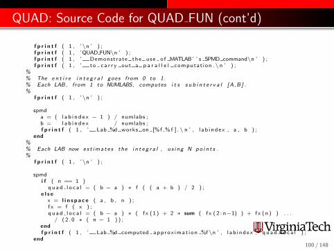
QUAD: Source Code for QUAD FUN (cont’d)

f p r i n t f ( 1 , ’\n ’ ) ;f p r i n t f ( 1 , ’QUAD FUN\n ’ ) ;f p r i n t f ( 1 , ’ Demonstrate the use o f MATLAB ’ ’ s SPMD command\n ’ ) ;f p r i n t f ( 1 , ’ to c a r r y out a p a r a l l e l computat ion .\n ’ ) ;

%% The e n t i r e i n t e g r a l goes from 0 to 1 .% Each LAB, from 1 to NUMLABS, computes i t s s u b i n t e r v a l [A ,B ] .%

f p r i n t f ( 1 , ’\n ’ ) ;

spmda = ( l a b i n d e x − 1 ) / numlabs ;b = l a b i n d e x / numlabs ;f p r i n t f ( 1 , ’ Lab %d works on [%f ,% f ] .\ n ’ , l a b i nd e x , a , b ) ;

end%% Each LAB now e s t ima t e s the i n t e g r a l , u s i n g N po i n t s .%

f p r i n t f ( 1 , ’\n ’ ) ;

spmdi f ( n == 1 )

q u a d l o c a l = ( b − a ) ∗ f ( ( a + b ) / 2 ) ;e l s e

x = l i n s p a c e ( a , b , n ) ;f x = f ( x ) ;q u a d l o c a l = ( b − a ) ∗ ( f x (1 ) + 2 ∗ sum ( f x ( 2 : n−1) ) + f x ( n ) ) . . .

/ ( 2 . 0 ∗ ( n − 1 ) ) ;endf p r i n t f ( 1 , ’ Lab %d computed app rox imat i on %f\n ’ , l a b i nd e x , q u a d l o c a l ) ;

end100 / 148

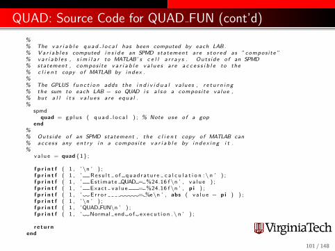
QUAD: Source Code for QUAD FUN (cont’d)

%% The v a r i a b l e q u a d l o c a l has been computed by each LAB .% Va r i a b l e s computed i n s i d e an SPMD sta tement a r e s t o r e d as ” compos i t e ”% v a r i a b l e s , s i m i l a r to MATLAB’ s c e l l a r r a y s . Out s ide o f an SPMD% statement , compos i t e v a r i a b l e v a l u e s a r e a c c e s s i b l e to the% c l i e n t copy o f MATLAB by i ndex .%% The GPLUS f u n c t i o n adds the i n d i v i d u a l v a l u e s , r e t u r n i n g% the sum to each LAB − so QUAD i s a l s o a compos i t e va lue ,% but a l l i t s v a l u e s a r e equa l .%

spmdquad = gp l u s ( q u a d l o c a l ) ; % Note use o f a gop

end%% Outs ide o f an SPMD statement , the c l i e n t copy o f MATLAB can% ac c e s s any en t r y i n a compos i t e v a r i a b l e by i n d e x i n g i t .%

v a l u e = quad{1} ;

f p r i n t f ( 1 , ’\n ’ ) ;f p r i n t f ( 1 , ’ R e s u l t o f quad ra tu r e c a l c u l a t i o n :\n ’ ) ;f p r i n t f ( 1 , ’ Es t imate QUAD = %24.16 f\n ’ , v a l u e ) ;f p r i n t f ( 1 , ’ Exact v a l u e = %24.16 f\n ’ , p i ) ;f p r i n t f ( 1 , ’ E r r o r = %e\n ’ , abs ( v a l u e − p i ) ) ;f p r i n t f ( 1 , ’\n ’ ) ;f p r i n t f ( 1 , ’QUAD FUN\n ’ ) ;f p r i n t f ( 1 , ’ Normal end o f e x e c u t i o n .\n ’ ) ;

r e t u r nend

101 / 148



QUAD Example

Distributed Arrays


IMAGE Example

CONTRAST Example

CONTRAST2: Messages

Batch Computing

Conclusion

102 / 148

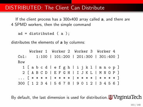
DISTRIBUTED: The Client Can Distribute

If the client process has a 300x400 array called a, and there are4 SPMD workers, then the simple command

ad = distributed ( a );

distributes the elements of a by columns:

Worker 1 Worker 2 Worker 3 Worker 4

Col: 1:100 | 101:200 | 201:300 | 301:400 ]

Row

1 [ a b c d | e f g h | i j k l | m n o p ]

2 [ A B C D | E F G H | I J K L | M N O P ]

... [ * * * * | * * * * | * * * * | * * * * ]

300 [ 1 2 3 4 | 5 6 7 8 | 9 0 1 2 | 3 4 5 6 ]

By default, the last dimension is used for distribution.

103 / 148

DISTRIBUTED: Workers Can Get Their Part

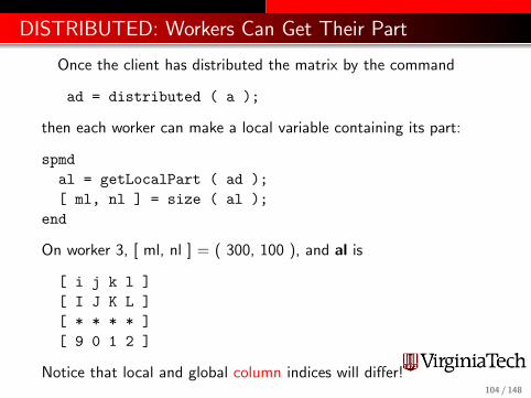
Once the client has distributed the matrix by the command

ad = distributed ( a );

then each worker can make a local variable containing its part:

spmd

al = getLocalPart ( ad );

[ ml, nl ] = size ( al );

end

On worker 3, [ ml, nl ] = ( 300, 100 ), and al is

[ i j k l ]

[ I J K L ]

[ * * * * ]

[ 9 0 1 2 ]

Notice that local and global column indices will differ!104 / 148

DISTRIBUTED: The Client Can Collect Results

The client can access any worker’s local part by using curlybrackets. Thus it could copy what’s on worker 3 by

worker3_array = al{3};

However, it’s likely that the client simply wants to collect all theparts and put them back into one normal Matlab array. If thelocal arrays are simply column-sections of a 2D array:

a2 = [ al{:} ]

Suppose we had a 3D array whose third dimension was 3, and wehad distributed it as 3 2D arrays. To collect it back:

a2 = al{1};

a2(:,:,2) = al{2};

a2(:,:,3) = al{3};

105 / 148

DISTRIBUTED: Methods to Gather Data

Instead of having an array created on the client and distributedto the workers, it is possible to have a distributed array constructedby having each worker build its piece. The result is still adistributed array, but when building it, we say we are building acodistributed array.

Codistributing the creation of an array has several advantages:

1 The array might be too large to build entirely on one core (orprocessor);

2 The array is built faster in parallel;

3 You avoid the communication cost of distributing it.

106 / 148

DISTRIBUTED: Accessing Distributed Arrays

The command al = getLocalPart ( ad ) makes a local copy ofthe part of the distributed array residing on each worker. Althoughthe workers could reference the distributed array directly, the localpart has some uses:

references to a local array are faster;

the worker may only need to operate on the local part; thenit’s easier to write al than to specify ad indexed by theappropriate subranges.

The client can copy a distributed array into a “normal” arraystored entirely in its memory space by the command

a = gather ( ad );

or the client can access and concatenate local parts.

107 / 148

DISTRIBUTED: Conjugate Gradient Setup

Because many Matlab operators and functions can automaticallydetect and deal with distributed data, it is possible to writeprograms that carry out sophisticated algorithms in which thecomputation never explicitly worries about where the data is!

The only tricky part is distributing the data initially, or gatheringthe results at the end.

Let us look at a conjugate gradient code which has been modifiedto deal with distributed data.

Before this code is executed, we assume the user has requestedsome number of workers, using the interactive parpool or indirectbatch command. (R2013b and later can do this automatically).

108 / 148

DISTRIBUTED: Conjugate Gradient Setup

% Sc r i p t to i n voke con j uga t e g r a d i e n t s o l u t i o n% f o r s p a r s e d i s t r i b u t e d ( or not ) a r r a y%

N = 1000 ;nnz = 5000 ;r c = 1/10 ; % r e c i p r o c a l c o n d i t i o n number

A = sprandsym (N, nnz/Nˆ2 , rc , 1 ) ; % symmetr ic , p o s i t i v e d e f i n i t eA = d i s t r i b u t e d (A ) ;%A = d i s t r i b u t e d . sprandsym ( ) i s not a v a i l a b l e

b = sum (A, 2 ) ;% f p r i n t f ( 1 , ’\n i s d i s t r i b u t e d ( b ) : %2 i \n ’ , i s d i s t r i b u t e d ( b ) ) ;

[ x , e norm ] = cg emc ( A, b ) ;

f p r i n t f ( 1 , ’ E r r o r r e s i d u a l : %8.4 e \n ’ , e norm {1}) ;

np = 10 ;f p r i n t f ( 1 , ’ F i r s t few x v a l u e s : \n ’ ) ;f p r i n t f ( 1 , ’ x ( %02 i ) = %8.4e \n ’ , [ 1 : np ; ga th e r ( x ( 1 : np ) ) ’ ] ) ;

sprandsym sets up a sparse random symmetric array A.distributed ‘casts’ A to a distributed array on the workers.Why do we write e norm{1} & gather(x) ?

109 / 148

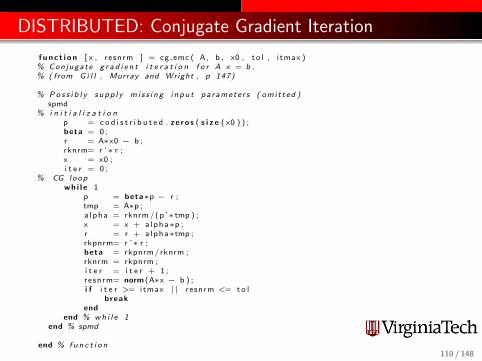
DISTRIBUTED: Conjugate Gradient Iteration

f u n c t i o n [ x , resnrm ] = cg emc ( A, b , x0 , t o l , i tmax )% Conjugate g r a d i e n t i t e r a t i o n f o r A x = b ,% ( from G i l l , Murray and Wright , p 147)

% Po s s i b l y s upp l y m i s s i n g i npu t pa ramete r s ( omi t ted )spmd

% i n i t i a l i z a t i o np = c o d i s t r i b u t e d . z e r o s ( s i z e ( x0 ) ) ;beta = 0 ;r = A∗x0 − b ;rknrm= r ’∗ r ;x = x0 ;i t e r = 0 ;

% CG loopw h i l e 1

p = beta∗p − r ;tmp = A∗p ;a lpha = rknrm /(p ’∗ tmp ) ;x = x + a lpha∗p ;r = r + a lpha∗tmp ;rkpnrm= r ’∗ r ;beta = rkpnrm/ rknrm ;rknrm = rkpnrm ;i t e r = i t e r + 1 ;resnrm= norm (A∗x − b ) ;i f i t e r >= itmax | | resnrm <= t o l

breakend

end % wh i l e 1end % spmd

end % fun c t i o n110 / 148

DISTRIBUTED: Comment

In cg emc.m, we can remove the spmd block and simply invokedistributed(); the operational commands don’t change.

There are several comments worth making:

The communication overhead can be severely increased

Not all Matlab operators have been extended to work withdistributed memory. In particular, (the last time we asked),the backslash or “linear solve” operator x=A\b can’t be usedyet for sparse distributed arrays.

Getting “real” data (as opposed to matrices full of randomnumbers) properly distributed across multiple processorsinvolves more choices and more thought than is suggested bythe conjugate gradient example !

111 / 148



QUAD Example

Distributed Arrays


IMAGE Example

CONTRAST Example

CONTRAST2: Messages

Batch Computing

Conclusion

112 / 148

DISTRIBUTED: Linear Boundary Value Problem

In the next example, we demonstrate a mixed approach whereinthe stiffness matrix (K) is initially constructed as acodistributed array on the workers. Each worker then modifies itslocalPart, and also assembles the local contribution to theforcing term (F). The local forcing arrays are then used to build acodistributed array.

113 / 148

DISTRIBUTED: FD LBVP script

%% FD LBVP SCRIPT i n v o k e s the f u n c t i o n f d l b v p f u n%% L i c e n s i n g :%% This code i s d i s t r i b u t e d under the GNU LGPL l i c e n s e .%% Author :%%% Gene C l i f f

n = 100 ; % g r i d paramete r

% De f i n e c o e f f i c i e n t f u n c t i o n s and boundary data f o r LBVPhnd l p = @( x ) 0 ;c q = 4 ; % p o s i t i v e f o r e xac t s o l u t i o n matchhnd l q = @( x ) c q ;c r = −4;h n d l r = @( x ) c r∗x ; % l i n e a r f o r e xac t s o l u t i o n match

a lpha = 0 ;beta = 2 ;

% Invoke s o l v e rf p r i n t f ( 1 , ’\n Invoke f d l b v p f u n \n ’ ) ;T = f d l b v p f u n (n , hnd l p , hnd l q , hnd l r , a lpha , beta ) ;

% gathe r the d i s t r i b u t e d s o l u t i o n on the c l i e n t p r o c e s s

Tg = ga the r (T) ; % When ’ batch ’ f i n i s h e s the ’ pool ’ i s c l o s e d% and d i s t r i b u t e d data i s l o s t

114 / 148

DISTRIBUTED: FD LBVP code

f u n c t i o n T = f d l b v p f u n (n , hnd l p , hnd l q , hnd l r , a lpha , beta )% F i n i t e−d i f f e r e n c e app rox imat i on to the BVP% T’ ’ ( x ) = p ( x ) T’ ( x ) + q ( x ) T( x ) + r ( x ) , 0 \ l e x \ l e 1% with T(0) = alpha , T(1) = beta

% Mod i f i ed :%% 2 March 2012%% Author :%% Gene C l i f f

% We use a un i fo rm g r i d w i th n i n t e r i o r g r i d p o i n t s% From Numer i ca l Ana l y s i s , Burden & Fa i r e s , 2001 , \S˜11 .3

h = 1/(n+1); ho2 = h /2 ; h2 = h∗h ;spmd

A = c o d i s t r i b u t e d . z e r o s (n , n ) ;locP = ge tLo c a lPa r t ( c o d i s t r i b u t e d . co l on (1 , n ) ) ; %index v a l s on l a bl ocP = locP ( : ) ;% make i t a column a r r a y

% Loop ove r columns e n t e r i n g u n i t y above / below the d i a g on a l e n t r y% a long wi th 2 p l u s the a p p r o p r i a t e q f u n c t i o n v a l u e s% Note tha t columns 1 and n a r e e x c e p t i o n s

f o r j j=locP ( 1 ) : locP ( end )% on the d i a g on a lA( j j , j j ) = 2 + h2∗ f e v a l ( hnd l q , j j ∗h ) ;% above the d i a g on a l

i f j j ˜= 1 ; A( j j −1, j j ) = −1+ho2∗ f e v a l ( hnd l p , ( j j −1)∗h ) ; end% below the d i a g ona li f j j ˜= n ; A( j j +1, j j ) = −1+ho2∗ f e v a l ( hnd l p , j j ∗h ) ; end

end

l o cF = −h2∗ f e v a l ( hnd l r , locP∗h ) ; % hnd l r okay f o r v e c t o r i n pu t

i f l a b i n d e x ( ) == 1locF ( 1 ) = locF ( 1 ) + a lpha∗(1+ho2∗ f e v a l ( hnd l p , h ) ) ;

endi f l a b i n d e x ( ) == numlabs ( ) ;

l o cF ( end ) = locF ( end ) + beta∗(1−ho2∗ f e v a l ( hnd l p , 1−h ) ) ;end

% co d i s t = c o d i s t r i b u t o r 1 d ( dim , p a r t i t i o n , g l o b a l s i z e ) ;c o d i s t = c o d i s t r i b u t o r 1 d (1 , c o d i s t r i b u t o r 1 d . u n s e t P a r t i t i o n , [ n , 1 ] ) ;F = c o d i s t r i b u t e d . b u i l d ( locF , c o d i s t ) ; % d i s t r i b u t e the a r r a y ( s )

end % spmd b lo ck

T = A\F ; % mld i v i d e i s d e f i n e d f o r c o d i s t r i b u t e d a r r a y s

115 / 148

DISTRIBUTED: FD LBVP code (cont’d)

l o cF = −h2∗ f e v a l ( hnd l r , locP∗h ) ; % hnd l r okay f o r v e c t o r i n pu t

i f l a b i n d e x ( ) == 1locF ( 1 ) = locF ( 1 ) + a lpha∗(1+ho2∗ f e v a l ( hnd l p , h ) ) ;

endi f l a b i n d e x ( ) == numlabs ( ) ;

l o cF ( end ) = locF ( end ) + beta∗(1−ho2∗ f e v a l ( hnd l p , 1−h ) ) ;end

% co d i s t = c o d i s t r i b u t o r 1 d ( dim , p a r t i t i o n , g l o b a l s i z e ) ;c o d i s t = c o d i s t r i b u t o r 1 d (1 , c o d i s t r i b u t o r 1 d . u n s e t P a r t i t i o n , [ n , 1 ] ) ;F = c o d i s t r i b u t e d . b u i l d ( locF , c o d i s t ) ; % d i s t r i b u t e the a r r a y ( s )

end % spmd b lo ck

T = A\F ; % mld i v i d e i s d e f i n e d f o r c o d i s t r i b u t e d a r r a y s

116 / 148

DISTRIBUTED: 2D Finite Element Heat Model

Next, we consider an example that combines SPMD anddistributed data to solve a steady state heat equations in 2D, usingthe finite element method. Here we demonstrate a differentstrategy for assembling the required arrays.

Each worker is assigned a subset of the finite element nodes. Thatworker is then responsible for constructing the columns of the(sparse) finite element matrix associated with those nodes.

Although the matrix is assembled in a distributed fashion, it has tobe gathered back into a standard array before the linear systemcan be solved, because sparse linear systems can’t be solved as adistributed array (yet).

This example is available as in the fem 2D heat folder.

117 / 148

DISTRIBUTED: The Grid & Node Coloring for 4 labs

118 / 148

DISTRIBUTED: Finite Element System matrix

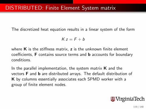
The discretized heat equation results in a linear system of the form

K z = F + b

where K is the stiffness matrix, z is the unknown finite elementcoefficients, F contains source terms and b accounts for boundaryconditions.

In the parallel implementation, the system matrix K and thevectors F and b are distributed arrays. The default distribution ofK by columns essentially associates each SPMD worker with agroup of finite element nodes.

119 / 148

DISTRIBUTED: Finite Element System Matrix

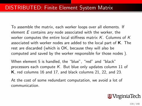
To assemble the matrix, each worker loops over all elements. Ifelement E contains any node associated with the worker, theworker computes the entire local stiffness matrix K . Columns of Kassociated with worker nodes are added to the local part of K. Therest are discarded (which is OK, because they will also becomputed and saved by the worker responsible for those nodes ).

When element 5 is handled, the “blue”, “red” and “black”processors each compute K . But blue only updates column 11 ofK, red columns 16 and 17, and black columns 21, 22, and 23.

At the cost of some redundant computation, we avoid a lot ofcommunication.

120 / 148

Assemble Codistributed Arrays - code fragment

spmd%% Set up c o d i s t r i b u t e d s t r u c t u r e%% Column p o i n t e r s and such f o r c o d i s t r i b u t e d a r r a y s .%

Vc = c o d i s t r i b u t e d . co l on (1 , n e qu a t i o n s ) ;lP = ge tLo c a lPa r t (Vc ) ;lP 1= lP ( 1 ) ; lP end = lP ( end ) ; %f i r s t and l a s t columns o f K on t h i s l a bc o d i s t V c = g e t C o d i s t r i b u t o r (Vc ) ; dPM = co d i s t V c . P a r t i t i o n ;

. . .% spa r s e a r r a y s on each l a b%

K lab = s p a r s e ( n equa t i on s , dPM( l a b i n d e x ) ) ;. . .

% Bu i l d the f i n i t e e l ement ma t r i c e s − Begin l oop ove r e l ement s%

f o r n e l =1: n e l emen t sn o d e s l o c a l = e conn ( n e l , : ) ;% which nodes a r e i n t h i s e l ement

% sub s e t o f nodes / columns on t h i s l a bl a b n o d e s l o c a l = e x t r a c t ( n o d e s l o c a l , lP 1 , lP end ) ;

. . . i f empty do noth ing , e l s e accumulate K lab , e t c endend % n e l

%% Assemble the ’ lab ’ p a r t s i n a c o d i s t r i b u t e d format .% syn tax f o r v e r s i o n R2009b

c o d i s t m a t r i x = c o d i s t r i b u t o r 1 d ( 2 , dPM, [ n equa t i on s , n e qu a t i o n s ] ) ;K = c o d i s t r i b u t e d . b u i l d ( K lab , c o d i s t m a t r i x ) ;

end % spmd

121 / 148

DISTRIBUTED: 2D Heat Equation - The Results

122 / 148



QUAD Example

Distributed Arrays


IMAGE Example

CONTRAST Example

CONTRAST2: Messages

Batch Computing

Conclusion

123 / 148

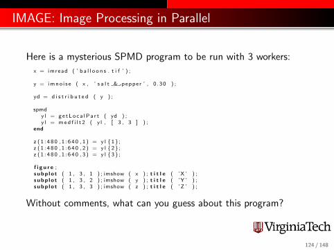
IMAGE: Image Processing in Parallel

Here is a mysterious SPMD program to be run with 3 workers:

x = imread ( ’ b a l l o o n s . t i f ’ ) ;

y = imno i s e ( x , ’ s a l t & pepper ’ , 0 .30 ) ;

yd = d i s t r i b u t e d ( y ) ;

spmdy l = ge tLo c a lPa r t ( yd ) ;y l = med f i l t 2 ( y l , [ 3 , 3 ] ) ;

end

z ( 1 : 4 80 , 1 : 6 4 0 , 1 ) = y l {1} ;z ( 1 : 4 8 0 , 1 : 6 4 0 , 2 ) = y l {2} ;z ( 1 : 4 8 0 , 1 : 6 4 0 , 3 ) = y l {3} ;

f i g u r e ;s u b p l o t ( 1 , 3 , 1 ) ; imshow ( x ) ; t i t l e ( ’X ’ ) ;s u b p l o t ( 1 , 3 , 2 ) ; imshow ( y ) ; t i t l e ( ’Y ’ ) ;s u b p l o t ( 1 , 3 , 3 ) ; imshow ( z ) ; t i t l e ( ’Z ’ ) ;

Without comments, what can you guess about this program?

124 / 148

IMAGE: Image → Noisy Image → Filtered Image

This filtering operation uses a 3x3 pixel neighborhood.We could blend all the noise away with a larger neighborhood.

125 / 148

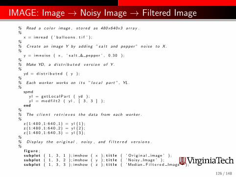
IMAGE: Image → Noisy Image → Filtered Image

% Read a c o l o r image , s t o r e d as 480 x640x3 a r r a y .%

x = imread ( ’ b a l l o o n s . t i f ’ ) ;%% Create an image Y by add ing ” s a l t and pepper ” n o i s e to X .%

y = imno i s e ( x , ’ s a l t & pepper ’ , 0 .30 ) ;%% Make YD, a d i s t r i b u t e d v e r s i o n o f Y .%

yd = d i s t r i b u t e d ( y ) ;%% Each worker works on i t s ” l o c a l p a r t ” , YL .%

spmdy l = ge tLo c a lPa r t ( yd ) ;y l = med f i l t 2 ( y l , [ 3 , 3 ] ) ;

end%% The c l i e n t r e t r i e v e s the data from each worker .%

z ( 1 : 4 80 , 1 : 6 4 0 , 1 ) = y l {1} ;z ( 1 : 4 8 0 , 1 : 6 4 0 , 2 ) = y l {2} ;z ( 1 : 4 8 0 , 1 : 6 4 0 , 3 ) = y l {3} ;

%% Di s p l a y the o r i g i n a l , no i s y , and f i l t e r e d v e r s i o n s .%

f i g u r e ;s u b p l o t ( 1 , 3 , 1 ) ; imshow ( x ) ; t i t l e ( ’ O r i g i n a l image ’ ) ;s u b p l o t ( 1 , 3 , 2 ) ; imshow ( y ) ; t i t l e ( ’ No i sy Image ’ ) ;s u b p l o t ( 1 , 3 , 3 ) ; imshow ( z ) ; t i t l e ( ’ Median F i l t e r e d Image ’ ) ;

126 / 148



QUAD Example

Distributed Arrays


IMAGE Example

CONTRAST Example

CONTRAST2: Messages

Batch Computing

Conclusion

127 / 148

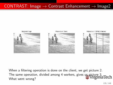
CONTRAST: Image → Contrast Enhancement → Image2

%% Get 4 SPMD worke r s%

pa rpoo l open 4%% Read an image%

x = imageread ( ’ s u r f s u p . t i f ’ ) ;%% Since the image i s b l a c k and white , i t w i l l be d i s t r i b u t e d by columns%

xd = d i s t r i b u t e d ( x ) ;%% Each worker enhances the c o n t r a s t on i t s p o r t i o n o f the p i c t u r e%

spmdx l = ge tLo c a lPa r t ( xd ) ;x l = n l f i l t e r ( x l , [ 3 , 3 ] , @con t r a s t enhance ) ;x l = u i n t 8 ( x l ) ;

end%% Concatenate the s ubma t r i c e s to as semb le the whole image%

xf spmd = [ x l {:} ] ;

p a r poo l / d e l e t e

128 / 148


When a filtering operation is done on the client, we get picture 2.The same operation, divided among 4 workers, gives us picture 3.What went wrong?

129 / 148


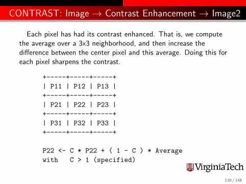
Each pixel has had its contrast enhanced. That is, we computethe average over a 3x3 neighborhood, and then increase thedifference between the center pixel and this average. Doing this foreach pixel sharpens the contrast.

+-----+-----+-----+

| P11 | P12 | P13 |

+-----+-----+-----+

| P21 | P22 | P23 |

+-----+-----+-----+

| P31 | P32 | P33 |

+-----+-----+-----+

P22 <- C * P22 + ( 1 - C ) * Average

with C > 1 (specified)

130 / 148


When the image is divided by columns among the workers,artificial internal boundaries are created. The nlfilter algorithmturns any pixel lying along the boundary to white. (The samething happened on the client, but we didn’t notice!)

Worker 1 Worker 2

+-----+-----+-----+ +-----+-----+-----+ +----

| P11 | P12 | P13 | | P14 | P15 | P16 | | P17

+-----+-----+-----+ +-----+-----+-----+ +----

| P21 | P22 | P23 | | P24 | P25 | P26 | | P27

+-----+-----+-----+ +-----+-----+-----+ +----

| P31 | P32 | P33 | | P34 | P35 | P36 | | P37

+-----+-----+-----+ +-----+-----+-----+ +----

| P41 | P42 | P43 | | P44 | P45 | P46 | | P47

+-----+-----+-----+ +-----+-----+-----+ +----

Dividing up the data has created undesirable artifacts!131 / 148


The result is spurious lines on the processed image.

132 / 148



QUAD Example

Distributed Arrays


IMAGE Example

CONTRAST Example

CONTRAST2: Messages

Batch Computing

Conclusion

133 / 148

CONTRAST2: Workers Need to Communicate

The spurious lines would disappear if each worker could just beallowed to peek at the last column of data from the previousworker, and the first column of data from the next worker.

Just as in MPI, Matlab includes commands that allow workers toexchange data.

The command we would like to use is labSendReceive() whichcontrols the simultaneous transmission of data from all the workers.

data_received = labSendReceive ( to, from, data_sent );

134 / 148

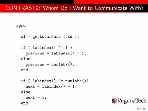
CONTRAST2: Whom Do I Want to Communicate With?

spmd

xl = getLocalPart ( xd );

if ( labindex() ~= 1 )

previous = labindex() - 1;

else

previous = numlabs();

end

if ( labindex() ~= numlabs())

next = labindex() + 1;

else

next = 1;

end

135 / 148

CONTRAST2: First Column Left, Last Column Right

column = labSendReceive ( previous, next, xl(:,1) );

if ( labindex() < numlabs() )

xl = [ xl, column ];

end

column = labSendReceive ( next, previous, xl(:,end) );

if ( 1 < labindex() )

xl = [ column, xl ];

end

136 / 148

CONTRAST2: Filter, then Discard Extra Columns

xl = nlfilter ( xl, [3,3], @enhance_contrast );

if ( labindex() < numlabs() )

xl = xl(:,1:end-1);

end

if ( 1 < labindex() )

xl = xl(:,2:end);

end

xl = uint8 ( xl );

end

137 / 148

CONTRAST2: Image → Enhancement → Image2

Four SPMD workers operated on columns of this image.Communication was allowed using labSendReceive.

138 / 148



QUAD Example

Distributed Arrays


IMAGE Example

CONTRAST Example

CONTRAST2: Messages

Batch Computing

Conclusion

139 / 148

BATCH: Indirect Execution

We can run quick, local interactive jobs using the matlabpool orparpool command to get parallel workers.

The batch command is an alternative which allows you to executea Matlab script (using either parfor or spmd statements) in thebackground on your desktop...or on a remote machine.

The batch command includes a matlabpool or pool argumentthat allows you to request a given number of workers.

For remote jobs, the number of cores or processors you are askingfor is the matlabpool plus one, because of the client.

140 / 148

BATCH: Contrast2

Running contrast2 on NewRiver and locally:

% Run on Ithaca

job = batch ( ’contrast2_script’, ...

’Profile’, ’newriver_R2015b’, ...

’CaptureDiary’, true, ...

’AttachedFiles’, { ’contrast2_fun’, ’contrast_enhance’, ’surfsup.tif’ }, ...

’CurrentDirectory’, ’.’, ...

’pool’, n );

% Run locally

x = imread ( ’surfsup.tif’ );

xf = nlfilter ( x, [3,3], @contrast_enhance );

xf = uint8 ( xf );

% Wait for NewRiver job to complete

wait ( job );

% Load results from NewRiver job

load ( job );

141 / 148

BATCH: Contrast2

Notes:

We need to include both scripts and the input filesurfsup.tif in the AttachedFiles flag

We can do some work before issuing wait()

We leverage two kinds of parallelism:

Parallel (using spmd) on an ARC ClusterRun locally while job is running on an ARC Cluster

142 / 148



QUAD Example

Distributed Arrays


IMAGE Example

CONTRAST Example

CONTRAST2: Messages

Batch Computing

Conclusion

143 / 148


The QUAD example showed a simple problem that could be doneas easily with SPMD as with PARFOR. We just needed to learnabout composite variables!

The CONJUGATE GRADIENT example showed that manyMatlab operations work for distributed arrays, a kind of arraystorage scheme associated with SPMD.

The LBVP & FEM 2D HEAT examples show how to constructlocal arrays and assemble these to codistributed arrays. Thisenables treatment of very large problems.

The IMAGE and CONTRAST examples showed us problems whichcan be broken up into subproblems to be dealt with by SPMDworkers. We also saw that sometimes it is necessary for theseworkers to communicate, using a simple message-passing system.

144 / 148

CONCLUSION: VT MATLAB LISTSERV

There is a local LISTSERV for people interested in MATLAB onthe Virginia Tech campus. We try not to post messages hereunless we really consider them of importance!

Important messages include information about workshops, specialMATLAB events, and other issues affecting MATLAB users.

To subscribe to this email list, send a blank email to

[email protected]

The subject and body of the message should both be empty.

145 / 148

CONCLUSION: Where is it?

Matlab Parallel Computing Toolbox Product Documentationhttp://www.mathworks.com/help/toolbox/distcomp/

Gaurav Sharma, Jos Martin,MATLAB: A Language for Parallel Computing, InternationalJournal of Parallel Programming,Volume 37, Number 1, pages 3-36, February 2009.

An Adobe PDF with these notes, along with a zipped-foldercontaining the Matlab codes can be downloaded from theARC website at

http://www.arc.vt.edu/matlab#resources

146 / 148

AFTERWORD: PMODE

PMODE allows interactive parallel execution ofMatlabcommands. PMODE achieves this by defining and submitting aparallel job, and it opens a Parallel Command Window connectedto the labs running the job. The labs receive commands entered inthe Parallel Command Window, process them, and send thecommand output back to the Parallel Command Window.

pmode start ’local’ 2 will initiate pmode; pmode exit willdelete the parallel job and end the pmode session

This may be a useful way to experiment with computations on thelabs.

147 / 148

THE END

Please complete the evaluation form

Thanks

148 / 148

Parallel MATLAB at VT - Virginia Tech · At VT, the concurrent ... Setting up intracluster...

Documents

Transcript of Parallel MATLAB at VT - Virginia Tech · At VT, the concurrent ... Setting up intracluster...