Parallel Data Analysis Directly on Scientific File Formats

Spyros Blanas 1 Kesheng Wu 2 Surendra Byna 2 Bin Dong 2 Arie Shoshani 2

1 The Ohio State University 2 Lawrence Berkeley National Laboratory

blanas.2@osu.edu {kwu, sbyna, dbin, ashosani}@lbl.gov

ABSTRACT

Scientific experiments and large-scale simulations producemassive amounts of data. Many of these scientific datasetsare arrays, and are stored in file formats such as HDF5and NetCDF. Although scientific data management systems,such as SciDB, are designed to manipulate arrays, there arechallenges in integrating these systems into existing analy-sis workflows. Major barriers include the expensive task ofpreparing and loading data before querying, and convert-ing the final results to a format that is understood by theexisting post-processing and visualization tools. As a con-sequence, integrating a data management system into anexisting scientific data analysis workflow is time-consumingand requires extensive user involvement.

In this paper, we present the design of a new scientificdata analysis system that efficiently processes queries di-rectly over data stored in the HDF5 file format. This designchoice eliminates the tedious and error-prone data loadingprocess, and makes the query results readily available to thenext processing steps of the analysis workflow. Our designleverages the increasing main memory capacities found insupercomputers through bitmap indexing and in-memoryquery execution. In addition, query processing over theHDF5 data format can be effortlessly parallelized to utilizethe ample concurrency available in large-scale supercomput-ers and modern parallel file systems. We evaluate the per-formance of our system on a large supercomputing systemand experiment with both a synthetic dataset and a realcosmology observation dataset. Our system frequently out-performs the relational database system that the cosmologyteam currently uses, and is more than 10× faster than Hivewhen processing data in parallel. Overall, by eliminatingthe data loading step, our query processing system is moreeffective in supporting in situ scientific analysis workflows.

1. INTRODUCTIONThe volume of scientific datasets has been increasing rapidly.Scientific observations, experiments, and large-scale simula-tions in many domains, such as astronomy, environment,

(c) 2014 Association for Computing Machinery. ACM acknowledges that this con-

tribution was authored or co-authored by an employee, contractor or affiliate of the

United States government. As such, the United States Government retains a nonexclu-

sive, royalty-free right to publish or reproduce this article, or to allow others to do so,

for Government purposes only.

SIGMOD/PODS’14, June 22 - 27 2014, Snowbird, UT, USA.

Copyright 2014 ACM 978-1-4503-2376-5/14/06...$15.00.

http://dx.doi.org/10.1145/2588555.2612185 ...$15.00.

and physics, produce massive amounts of data. The size ofthese datasets typically ranges from hundreds of gigabytesto tens of petabytes. For example, the Intergovernmen-tal Panel on Climate Change (IPCC) multi-model CMIP-5archive, which is used for the AR-5 report [22], contains over10 petabytes of climate model data. Scientific experiments,such as the LHC experiment routinely store many gigabytesof data per second for future analysis. As the resolution ofscientific data is increasing rapidly due to novel measure-ment techniques for experimental data and computationaladvances for simulation data, the data volume is expectedto grow even further in the near future.

Scientific data are often stored in data formats that sup-port arrays. The Hierarchical Data Format version 5 (HDF5)[2] and the Network Common Data Form (NetCDF) [1] aretwo well-known scientific file formats for array data. Thesefile formats are containers for collections of data objects andmetadata pertaining to each object. Scientific data stored inthese formats is accessed through high-level interfaces, andthe library can transparently optimize the I/O dependingon the particular storage environment. Applications thatuse these data format libraries can achieve the peak I/Obandwidth from parallel file systems on large supercomput-ers [6]. These file formats are well-accepted for scientificcomputing and are widely supported by visualization andpost-processing tools.

The analysis of massive scientific datasets is critical forextracting valuable scientific information. Often, the mostvital pieces of information for scientific insights consist ofa small fraction of these massive datasets. Because thesescientific file format libraries are optimized for storing andretrieving consecutive parts of the data, there are severalinefficiencies in accessing individual elements. It is impor-tant for the scientific data analysis systems to support suchselective data accesses efficiently.

Additionally, scientific file format libraries commonly lacksophisticated query interfaces. For example, searching fordata that satisfy a given condition in an HDF5 file todayrequires accessing the entire dataset and sifting through thedata for values that satisfy the condition. Moreover, usersanalyzing the data need to write custom code to perform thisstraightforward operation. In comparison, with a databasemanagement system (DBMS), searches can be expressed asdeclarative SQL queries. Existing high-level interfaces forscientific file formats do not support such declarative query-ing and management capabilities.

Scientific data management and analysis systems, such asSciDB [11], SciQL [39], and ArrayStore [30], have been re-

cently developed to manage and query scientific data storedas arrays. However, there are major challenges in integrat-ing these systems into scientific data production and analysisworkflows. In particular, in order to benefit from the query-ing capabilities and the storage optimizations of a scientificdata management system, the data need to be prepared intoa format that the system can load. Preparing and loadinglarge scientific datasets is a tedious and error-prone task fora domain scientist to perform, and hurts scientific productiv-ity during exploratory analysis. Moreover, after executingqueries in a data management system, the scientists needto convert the results into a file format that is understoodby other tools for further processing and visualization. Asa result, the integration of data management systems in sci-entific data processing workflows has been scarce and theusers frequently revert to inefficient and ad hoc methods fordata analysis.

In this paper, we describe the design of a prototype sys-tem, called SDS/Q, that can process queries directly overdata that are stored in the HDF5 file format1. SDS/Q standsfor Scientific Data Services [18], and we describe the Queryengine component. Our goal is to support data analysis di-rectly on file formats that are familiar to scientific users. Thechoice of the HDF5 storage format is based on its popularity.

SDS/Q is capable of executing SQL queries on data storedin the HDF5 file format in an in situ fashion, which elim-inates the need for expensive data preparation and loadingprocesses. While query processing in database systems is amatured concept, developing the same level of support onarray storage formats directly is a challenge. The capabilityto perform complex operations, such as JOIN operations ondifferent HDF5 datasets increases the complexity further.To optimize sifting through massive amounts of data, wedesigned SDS/Q to use the parallelism available on largesupercomputer systems, and we have used in-memory query-ing execution and bitmap indexing to take advantage of theincreasing memory capacities.

We evaluate the performance of SDS/Q on a large super-computing system and experiment with a real cosmologyobservations database, called the Palomar Transient Fac-tory (PTF), which is a PostgreSQL database. The schemaand the queries running on PostgreSQL were already op-timized by a professional database administrator, so thischoice gives us a realistic comparison baseline. Our testsshow that our system frequently performs better than Post-greSQL without the laborious process of preparing and load-ing the original data into the data management system. Inaddition, SDS/Q can effortlessly speed up query processingby requesting more processors from the supercomputer, andoutperforms Hive by more than 10× on the same cosmologydataset. This ease of parallelization is an important featureof SDS/Q for processing scientific data.

The following are the contributions of our work:

• We design and develop a prototype in situ relationalquery processing system for querying scientific datain the HDF5 file format. Our prototype system caneffortlessly speed up query processing by leveraging themassive parallelism of modern supercomputer systems.

1The ability to query data directly in their native file for-mat has been referred to as in situ processing in the datamanagement community [3].

• We combine an in-memory query execution engine andbitmap indexing to significantly improve performancefor highly selective queries over HDF5 data.

• We systematically explore the performance of the pro-totype system when processing data in the HDF5 fileformat.

• We demonstrate that in situ SQL query processingoutperforms PostgreSQL when querying a real cosmol-ogy dataset, and is more than 10× faster than Hivewhen querying this dataset in parallel.

The remainder of the paper is structured as follows. First,we discuss related work on scientific data management inSection 2. Then, in Section 3, we describe the SDS/Q pro-totype. Section 4 follows with a description of the experi-mental setup and presents the performance evaluation. Weconclude and briefly discuss future work in Section 5.

2. RELATED WORKSeveral technologies have been proposed to make scientificdata manipulation more elegant and efficient. Among thesetechnologies, Array Query Language (AQL) [24], RasDaMan[5], ArrayDB [25], GLADE [16], Chiron [26], Relational Ar-ray Mapping (RAM) [34], ArrayStore [30], SciQL [39], Mon-etDB [21], and SciDB [11] have gained prominence in analyz-ing scientific data. Libkin et al. [24] propose a declarativequery language, called Array Query Language (AQL), formulti-dimensional arrays. AQL treats arrays as functionsfrom index sets to values rather than as collection types.Libkin et al. provide readers/writers for data exchange for-mats like NetCDF to tie their system to legacy scientificdata. ArrayStore [30] is a storage manager for storing arraydata using regular and arbitrary chunking strategies. Array-Store supports full scan, subsampling, join, and clusteringoperations on array data.

Scientific data management systems can operate on ar-rays and support declarative querying capabilities. Ras-DaMan [5] is a domain-independent array DBMS for multi-dimensional arrays. It provides a SQL-based array querylanguage, called RasQL, for optimizing data storage, trans-fer, and query execution. ArrayDB [25] is a prototype ar-ray database system that provides Array Manipulation Lan-guage (AML). AML is customizable to support a wide-varietyof domain-specific operations on arrays stored in a database.MonetDB [21] is a column-store DBMS supporting applica-tions in data mining, OLAP and data warehousing. Rela-tional Array Mapping (RAM) [34] and SciQL [39] are im-plemented on top of MonetDB to take advantage of thevertically-fragmented storage model and other optimizationsfor scientific data. SciQL provides a SQL-based declarativequery language for scientific data stored either in tables orarrays. SciDB [11] is a shared-nothing parallel database sys-tem for processing multidimensional dense arrays. SciDBsupports both the Array Functional Language (AFL) andthe Array Query Language (AQL) for analyzing array data.Although these systems can process array data, scientificdatasets stored in “legacy” file formats, such as HDF5 andNetCDF, have to be prepared and loaded into these datasystems first in order to reap the benefits of their rich query-ing functionality and performance. In contrast, our solutionprovides in situ analysis support, and allows users to analyzedata using SQL queries directly over the HDF5 scientific fileformat.

Figure 1: Overview of SDS/Q, the querying compo-nent of a prototype scientific data management sys-tem. The new components are highlighted in gray.

There have also been efforts to query data in their orig-inal file formats. Alagiannis et al. eliminate the data loadstep for PostgreSQL and run queries directly over comma-separated value files [3]. In this paper, we adapt the po-sitional map Alagiannis et al. proposed and index HDF5data (see Algorithm 2) and experimentally evaluate its suit-ability for SDS/Q in Section 4.4.3. Several recent effortspropose techniques to support efficient selections and ag-gregations over scientific data formats, and are importantbuilding blocks for advanced SDS/Q querying capabilities,such as joins between different datasets. Wang et al. [36] pro-pose to automatically annotate HDF5 files with metadata toallow users to query data with a SQL-like language. Fast-Bit [37], an open-source bitmap indexing technology, sup-ports some features of in situ analysis as indexes can bequeried and stored alongside the original data. FastQuery[17], implemented on top of FastBit, parallelizes FastBit’sindex generation and query processing operations, and pro-vides a programming interface for executing simple lookups.DIRAQ [23] is a parallel data encoding and reorganizationtechnique that supports range queries while data is beingproduced by scientific simulations. FlexQuery [40] is an-other proposed system to perform range queries to supportvisualization of data while the data is being generated. Su etal. [32] implemented user-defined subsetting and aggregationoperations on NetCDF data. Finally, several MapReduce-based solutions have been proposed to query scientific data.SciHadoop [12] enables parallel processing through Hadoopfor data stored in the NetCDF format. Wang et al. [35]propose a unified scientific data processing API to enableMapReduce-style processing directly on different scientificfile formats.

3. A SCIENTIFIC DATA ANALYSIS SYSTEMA scientist today uses a diverse set of tools for scientificcomputation and analysis, such as simulations, visualiza-tion tools, and custom scripts to process data. Scientificfile format libraries, however, lack the sophisticated query-

ing capabilities found in database management systems. Weaddress this shortcoming by adding relational querying ca-pabilities directly over data stored in the HDF5 file format.

Figure 1 shows an overview of SDS/Q, a prototype in situ

scientific data analysis system. Compared to a databasemanagement system, SDS/Q faces three unique technicalchallenges. First, SDS/Q relies on the HDF5 library for fastdata access. Section 3.1 presents how data are stored inand retrieved from the HDF5 file format. Second, SDS/Qdoes not have the opportunity to reorganize the original databecause legacy applications may manipulate the HDF5 filedirectly. SDS/Q employs external bitmap indexing to im-prove performance for highly selective queries, which is de-scribed in Section 3.2. Third, SDS/Q needs to leverage theabundant parallelism of large-scale supercomputers whichis exposed through a batch processing execution environ-ment. Section 3.3 describes how the query processing isparallelized across and within nodes, presents how HDF5data are ingested in parallel, and discusses the integrationof the bitmap indexing capabilities in the SDS/Q prototype.

3.1 Storing scientific data in HDF5The Hierarchical Data Format version 5 (HDF5) is a portablefile format and library for storing scientific data. The HDF5library defines an abstract data model, which includes files,data groups, datasets, metadata objects, datatypes, prop-erties, and links between objects. The parallel implemen-tation of the HDF5 library is designed to operate on largesupercomputers. This implementation relies on the MessagePassing Interface (MPI) [20] and on the I/O implementationof the MPI, known as MPI-IO [33]. The HDF5 library andthe MPI-IO layers of the parallel I/O subsystem offer var-ious performance tuning parameters to achieve peak I/Obandwidth on large-scale computing systems [6].

A key concept in HDF5 is the dataset, which is a multi-dimensional array of data elements. An HDF5 dataset cancontain basic datatypes, such as integers, floats, or charac-ters, as well as composite or user-defined datatypes. Theelements of an HDF5 dataset are either stored as a contin-uous stream of bytes in a file, or in a chunked form. Theelements within one chunk of an HDF5 dataset are storedcontiguously, but chunks may be scattered within the HDF5file. HDF5 datasets that represent variables from the sameevent or experiment can be structured as a group. Groups,in turn, can be contained in other groups and form a grouphierarchy.

An HDF5 dataset may be stored on disk in a number ofdifferent physical layouts. The HDF5 dataspace abstractiondecouples the logical data view at the application level fromthe physical representation of the data on disk. Throughthis abstraction, applications become more portable as theycan control the in-memory representation of scientific datawithout implementing endianness or dimensionality trans-formations for common operations, such as sub-setting, sub-sampling, and scatter-gather access. In addition, analysisbecomes more efficient, as applications can take advantageof transparent optimizations within the HDF5 library, suchas compression, without any modifications.

Reading data from the disk into the memory requires amapping between the source dataspace (the file dataspace,or filespace) and the destination dataspace (the memorydataspace, or memspace). The file and the memory datas-paces may have different shapes or sizes, and neither datas-

pace needs to be continuous. A mapping between datas-paces of the same shape but different size performs arraysub-setting. A mapping between dataspaces that hold thesame number of elements but have different shapes triggersan array transformation. Finally, mapping a non-continuousfilespace onto a continuous memspace performs a gather op-eration. Once a mapping has been set up, the H5Dread()

function of the HDF5 library loads the data from disk intomemory.

3.2 Indexing HDF5 dataIndexing is an essential tool for accelerating highly-selectivequeries in relational database management systems. Thesame is true for scientific data management systems [29].However, in order to work with scientific data files in situ,one mainly uses secondary indexes, as the original data recordscannot usually be reorganized. Other characteristics of sci-entific workloads include that the data is frequently append-only and that the accesses are read-dominant. Hence, theperformance of analytical queries is much more importantthan the performance of data manipulation queries. Bitmapindexing has been shown to be effective given the above sci-entific data characteristics [27]. The original bitmap indexdescribed by O’Neil [27] indexes each key value precisely andonly supports equality encoding. Researchers have since ex-tended bitmap indexing to support range encoding [14] andinterval encoding [15]. Scientific datasets often have a largenumber of distinct values which leads to large bitmap in-dexes. In many scientific applications, and especially dur-ing exploratory analysis, the constants involved in queriesare low precision numbers, such as 1-degree temperature in-crements. Binning techniques have been proposed to allowthe user to control the number of bitmaps produced, andindirectly control the index size. Compression is anothercommon technique to control the bitmap index sizes [38].

For this work we use FastBit, an open-source bitmap in-dexing library [37]. In addition to implementing many bitmapindexing techniques, FastBit also adopts techniques seen indata warehousing engines. For example, it organizes its datain a vertical organization and it implements cost-based opti-mization for dynamically selecting the most efficient execu-tion strategy among the possible ways of resolving a querycondition. Although FastBit is optimized for bitmap indexesthat fit in memory, it can handle bitmap indexes that arelarger than memory too. If a small part of an index file isneeded to resolve the relevant query condition, FastBit onlyretrieves the necessary part of the index files. FastBit alsomonitors its own memory usage and could free the unusedindexing data structures when the memory is needed forother operations. Most importantly, the FastBit softwarehas a feature that makes it particularly suitable for in situ

data analysis: its bitmap indexes are generated alongsidethe base data, without needing to reorganize the base files.

Probing the FastBit index on every lookup, however, isprohibitively expensive because many optimizations in theFastBit implementation aim to maximize throughput forbulk processing. Although these optimizations benefit cer-tain types of scientific data analysis, one needs to optimizefor latency to achieve good performance for highly selec-tive queries. To improve the efficiency of point lookups inSDS/Q, we have separated the index lookup operation intothree discrete actions: prepare(), refine() and perform().The first, prepare() is called once per query and permits

FastBit to optimize for static conditions, that is, conditionsthat are known or can be inferred from the query plan dur-ing initialization. In our existing prototype, these are joinconditions and user-defined predicates that can be pusheddown to the index. Once this initial optimization has beencompleted, the query execution engine invokes the refine()function to further restrict the index condition (for example,to look for a particular key value or key range). Because re-fine() may be invoked multiple times per lookup, we onlyallow the index condition to be passed in programmatically,as parsing a SQL statement would be prohibitively expen-sive. Finally, the engine invokes the perform() function todo the lookup. FastBit can choose to optimize the executionstrategy again prior to retrieving the data, if the optimiza-tion is deemed worthwhile.

3.2.1 Automatic index invalidation by in situ updates

SDS/Q maintains scientific data in their original formatfor in situ data analysis, and augments the raw scientificdata with indexing information for efficiency. By storing in-dexing information separately, legacy applications that di-rectly update or append scientific data through the HDF5library would render indexing information stale. As a con-sequence, analysis tasks that use indexes may miss newerdata and return wrong results. This would severely limitthe effectiveness of indexing for certain classes of applica-tions. To ensure the consistency of the index data in thepresence of updates, SDS/Q needs to detect that the orig-inal dataset has been modified or appended to, and act onthe knowledge that the index data are now stale.

We leverage the Virtual Object Layer (VOL) abstractionof the HDF5 library to intercept writes to HDF5 objects andto generate notifications when a dataset changes during in

situ processing. VOL allows users to customize how HDF5metadata structures and scientific data are represented ondisk. A VOL plugin acts as an intermediary between theHDF5 API and the actual driver that performs the I/O.Using VOL, we can intercept HDF5 I/O requests initiatedby legacy applications and notify SDS/Q to invalidate allindex data for the dataset in question. In the future, we planto avoid the expensive index regeneration step and updateindex data directly.

3.3 Analyzing scientific dataA key component of SDS/Q is a query execution enginethat ingests and analyzes data stored in the HDF5 format.The query engine is written in C++, and intermediate re-sults that are produced during query execution are stored inmemory. The engine accepts queries in the form of a physicalexecution plan, which is a tree of relational operators. TheHDF5 scan operator (described in detail in Section 3.3.3)retrieves elements from different HDF5 datasets and pro-duces relational tuples. An index scan operator can retrievedata from FastBit indexes. For additional processing, thequery engine currently supports a number of widely-used re-lational operators such as expression evaluation, projection,aggregation, and joins. Aggregations and joins on compositeattributes are also supported. We have implemented bothhash-based and sort-based aggregation and join operators,as the database research community is currently engagedin an ongoing debate about the merits of hash-based andsort-based methods for in-memory query execution [4].

The execution model is based on the iterator concept,which is pull-based, and is similar to the Volcano system[19]. All operators in our query engine have the same inter-face, which consists of: a start() function for initializationand operation-specific parameter passing (such as the keyrange for performing an index lookup), a next() functionfor retrieving data, and a stop() function for termination.Previous research has shown that retrieving one tuple at atime is prohibitively expensive [10], so the next() call re-turns an array of tuples to amortize the cost of functioncalls. The pull-based model allows operators to be pipelinedarbitrarily and effortlessly to evaluate complex query plansin our prototype system.

3.3.1 Parallelizing across nodes

A scientist analyzes large volumes of data by submittinga parallel job request to the supercomputer’s batch process-ing system. The request includes the number of nodes thatneed to be allocated before this job starts. When the analy-sis task is scheduled for execution, the mpirun utility is calledto spawn one SDS/Q process per node. The scan operatorsat the leaf level of the query tree partition the input usingthe MPI_comm_size() and MPI_comm_rank() functions to re-trieve the total number of processes and the unique identi-fier of this process, respectively. Each node then retrievesand processes a partition of the data, and synchronizes withother nodes in the supercomputer using MPI primitives suchas MPI_Barrier().

If intermediate results need to be shuffled across nodes tocomplete the query, SDS/Q leverages the shared disk archi-tecture of the supercomputer and shuffles data by writing toand reading from the parallel file system. For example, eachSDS/Q process participating in a broadcast hash join algo-rithm produces data in a staging directory in the parallel filesystem, and then every process builds a hash table by read-ing every file in the staging directory. Although disk I/Ois more expensive than native MPI communication primi-tives (such as MPI_Bcast() and MPI_Alltoall()), storingintermediate data in the parallel file system greatly simpli-fies fault tolerance and resource elasticity for our prototypesystem.

3.3.2 Parallelizing within a node

At the individual node level, the single SDS/Q processspawns multiple threads to fully utilize all the CPU coresof the compute node. We encapsulate thread creation andmanagement in a specialized operator, the parallelize op-erator. The main data structure for thread synchroniza-tion is a multi-producer, single-consumer queue: Multiplethreads produce intermediate results concurrently for all op-erators rooted under the parallelize operator in the querytree, but these intermediate results are consumed sequen-tially by the operator above the parallelize operator. Thestart() method spawns the desired number of threads, andreturns to the caller when all spawned threads have propa-gated the start() call to the subtree. The producer threadsstart working and push intermediate results to the queue.The next() method pops a result from the queue and re-turns it to the caller. The stop() method of the parallelize

operator propagates the stop() call to the entire subtree,and signals all threads to terminate.

By using multiple worker threads, and not multiple pro-cesses per node, all threads can efficiently exchange data,

Figure 2: The HDF5 scan operation. Chunks arearray regions that are stored contiguously on disk.For every HDF5 dataset di, each SDS/Q process op-erates on a unique subset of the array (the filespacefi). Every array subset is linearized in memory inthe one-dimensional memspace mi, which becomesone column of the final output.

Algorithm 1 The HDF5 scan operator

1: function start(HDF5 datasets {d1, . . . , dn}, int count)2: for each HDF5 dataset di do

3: open dataset di, verify data type and shape4: create filespace fi to cover this node’s di partition5: create memspace mi to hold count elements6: map mi on fi at element 07: end for

8: end function

9: function next()10: for each filespace fi do

11: call H5Dread() to populate memspace mi from fi12: copy memspace mi into column i of output buffer13: advance mapping of mi on fi by count elements14: if less than count elements remain in filespace fi then15: shrink memspace mi

16: end if

17: end for

18: end function

synchronize and share data structures through the commonprocess address space and not rely on expensive inter-processcommunication. For example, during a hash join, all threadscan synergistically share a single hash table, synchronize us-ing spinlocks, and access any hash bucket directly. (Thishash join variant has also been shown to use working mem-ory judiciously and perform well in practice [7].) If inter-mediate results need to be shuffled between threads duringquery processing (for example, for partitioning), threads ex-change pointers and read the data directly.

3.3.3 Ingesting data from the HDF5 library

The query engine ingests HDF5 data through the HDF5scan operator. The HDF5 scan operator reads a set of user-defined HDF5 datasets (each a multi-dimensional array) and“stitches”elements into a relational tuple. The HDF5 librarytransparently optimizes the data access pattern at the MPI-IO driver layer, while the query execution engine remainsoblivious to where the data is physically stored.

The HDF5 scan operation is described in Algorithm 1.The operation is initialized by calling the start() methodand providing two parameters: (1) a list of HDF5 datasets toaccess ({d1, d2, . . . , dn}), and (2) the desired output buffer

Algorithm 2 Positional map join

1: function start(Positional index idx, HDF5 datasets{d1, . . . , dn}, Join key JR from R, int count)

2: for each HDF5 dataset di do

3: open dataset di, verify data type and shape4: create empty sparse filespace fi5: end for

6: load idx in memory7: create empty hash table HT8: for each tuple r ∈ R do

9: pos← idx.lookup(πJR(r))

10: if join key πJR(r) found in idx then

11: expand all filespaces {fi} to cover element at pos12: store r in HT under join key πJR

(r)13: end if

14: end for

15: for each filespace fi do

16: create memspace mi to hold count elements17: map mi on fi at element 018: end for

19: allocate buffer BS to hold count elements20: end function

21: function next(Join key JS from S)22: for each dataset di do

23: call H5Dread() to populate memspace mi from fi24: copy memspace mi into column i of buffer BS

25: advance mapping of mi on fi by count elements26: end for

27: for each tuple s ∈ BS do

28: for each r in HT such that πJS(s) = πJR

(r) do

29: copy s ✶ r to output buffer30: end for

31: end for

32: end function

size (count). For example, consider a hypothetical atmo-spheric dataset shown in Figure 2. The user opens thetwo-dimensional HDF5 datasets “temperature” (d1), “pres-sure” (d2) and “wind velocity” (d3). Every process firstcomputes partitions of the dataset and constructs the two-dimensional filespaces {f1, f2, f3}, which define the array re-gion that will be analyzed by this process. Each processthen creates the one-dimensional memspaces {m1,m2,m3}to hold count elements. (The user defines how the multi-dimensional filespace fi is linearized in the one-dimensionalmemspace mi.) Finally, the HDF5 scan operator maps eachmemspace mi to the beginning of the filespace fi before re-turning to the caller of the start() function.

When the next() method is invoked, the HDF5 scan oper-ator iterates through each filespace fi in sequence and callsH5Dread() to retrieve elements from the filespace fi intomemspace mi. This way, the k-th tuple in the output bufferis the tuple (m1[k], m2[k], . . . ,mn[k]). Before returning thefilled output buffer to the caller, the operator checks if eachmemspace mi needs to be resized because insufficient ele-ments remain in the filespace fi.

We have experimentally observed that optimally sizing theoutput buffer of the HDF5 scan operator represents a trade-off between two antagonistic factors. The parallel filesystemand the HDF5 library are optimized for bulk transfers andhave high fixed overheads for each read. We have found thattransferring less than 4MB per H5Dread() call is very ineffi-cient. Amortizing these fixed costs over larger buffer sizes in-creases performance. On the other hand, buffer sizes greaterthan 256MB result in large intermediate results. This in-creases the memory management overhead, and causes finalresults to arrive unpredictably and in batches, instead of

Algorithm 3 Semi-join with FastBit index

1: function start(FastBit index idx, Predicate p on S, Joinkey JR from R, int count)

2: idx.prepare(p)3: create empty predicate q(·)4: create empty hash table HT5: for each tuple r ∈ R do

6: store r in HT under join key πJR(r)

7: q(·) ← q(·) ∨(

πJR(·) = πJR

(r))

8: end for

9: idx.refine(q)10: allocate buffer BS to hold count elements11: end function

12: function next(Join key JS from S)13: BS ← idx.perform(count)14: for each tuple s ∈ BS do

15: for each r in HT such that πJS(s) = πJR

(r) do

16: copy s ✶ r to output buffer17: end for

18: end for

19: end function

continuously. Very large buffer sizes, therefore, eliminatemany of the benefits of continuous pipelined query execu-tion [13]. We have experimentally found that a 32MB out-put buffer balances these two factors, and we use this outputbuffer size for our experiments in Section 4.

3.3.4 Positional map join

In addition to index scans, SDS/Q can use indexes toaccelerate join processing for in situ data processing. Ala-giannis et al. have proposed maintaining positional maps toremember the locations of attributes in text files and avoidthe expensive parsing and tokenization overheads [3]. Weextend the idea of maintaining positional information toquickly navigate through HDF5 data, and we exploit thisinformation for join processing. In particular, we use po-sitional information from a separate index file which stores(key, position) pairs, and use this information to create asparse filespace fi over the elements of interest in an HDF5dataset. Mapping a sparse filespace fi onto a continuousmemspace mi triggers the HDF5 gather operation, and theselected data elements are selectively retrieved from diskwithout loading the entire dataset.

Algorithm 2 describes the positional map join algorithm.R is the table that is streamed in from the next operator inthe query tree, and S is the table that the positional indexhas been built on. The algorithm first creates an emptysparse filespace fi for each dataset of interest and loads theentire positional map in memory (lines 2–7). The indexis probed with the join key of each input tuple, and if amatching position (pos) is found in the index, the inputtuple is stored in a hash table and the position is addedto the filespace fi (lines 8–14). When the next() methodis called, count elements at the selected positions in fi areretrieved from the HDF5 file and stored in buffer BS (lines22–26). Finally, a hash join is performed between BS andthe hash table (lines 27–31) and the results are returned tothe caller.

3.3.5 FastBit index semi-join

We now describe an efficient semi-join based index joinover the FastBit index (Algorithm 3). We assume that R isthe table that is streamed in from the operator below theFastBit semi-join operator, and S is the table that is stored

in the FastBit index. The FastBit index semi-join operatoraccepts: (1) the FastBit index file (idx), (2) an optional se-lection σ(·) to directly apply on the indexed table S, (3) thejoin key projection πj(·) and the columns of interest π(·) ofthe streamed input table R, and (4) the number of elementsthat the output buffer will return (count). The optional fil-tering condition σ(·) is passed to the initialization functionprepare() to allow FastBit to perform initial optimizationsfor static information in the query plan. As the input R isconsumed, the algorithm stores the input π(R) in a hash ta-ble, and adds the join keys πj(R) to the σj predicate. Whenthe entire build input has been processed, the σj predicate ispassed to the refine() method to further restrict the indexcondition before performing the index lookup. The algo-rithm’s next() method populates the BS buffer with count

tuples from FastBit and joins BS with the hash table.

4. EXPERIMENTAL SETUP AND RESULTSIn this section we evaluate the performance of the SDS/Qprototype for in situ analysis of scientific data. Since ourgoal is to provide SQL query processing capabilities directlyon scientific file formats, we looked for real scientific datasetsthat are already queried using SQL. We have chosen a Post-greSQL database that contains cosmological observation datafrom the Palomar Transient Factory (PTF) sky survey. Thepurpose of our experiments is to run the workload the sci-entists currently run on PostgreSQL, and compare the queryresponse time to running the same SQL queries on our SDS/Qsystem, which runs directly on top of HDF5. The advantageof taking this experimental approach is that the relationalschema has already been designed by the application scien-tists, and PostgreSQL has been tuned and optimized by anexpert database administrator. This makes our comparisonsmore realistic.

We conduct our experimental evaluation on the Carversupercomputer at the National Energy Research ScientificComputing Center (NERSC). We describe the NERSC in-frastructure in more detail in Section 4.1, and provide thedetails of our experimental methodology in Section 4.2. Wefirst evaluate the performance of reading data from the HDF5file format library through controlled experiments with asynthetic workload in Section 4.3. We complete the evalu-ation of our SDS/Q prototype using the PTF observationdatabase in Section 4.4.

4.1 Computational PlatformNERSC is a high-performance computing facility that servesa large number of scientific teams around the world. We usethe Carver system at NERSC for all our experiments, whichis an IBM iDataPlex cluster with 1,202 compute nodes. Themajority of these compute nodes have dual quad-core IntelXeon X5550 (“Nehalem”) 2.67 GHz processors, for a totalof eight cores per node, and 24 GB of memory. The nodeshave no local disk; the root file system resides in RAM, anduser data are stored in a parallel file system (GPFS).

Scientific applications run on the NERSC infrastructureas a series of batch jobs. The user submits a batch scriptto the scheduler that specifies (1) an executable to be run,(2) the number of nodes and processing cores that will beneeded to run the job, and (3) a wall-clock time limit, af-ter which the job will be terminated. When the requestedresources become available, the job starts running and thescheduler begins charging the user (in CPU hours) based on

the elapsed wall-clock time and the number of processingcores allocated to the job.

4.2 Experimental methodologyEvaluating system performance on large-scale shared infras-tructure poses some unique challenges, as ten-thousand-coreparallel systems such as the Carver system are rarely idle.Although the batch queuing system guarantees that a num-ber of compute nodes will be exclusively reserved to a partic-ular task, the parallel file system and the network intercon-nect offer no performance isolation guarantees. Scientificworkloads, in particular, commonly exhibit sudden burstsof I/O activity, such as when a large-scale simulation com-pletes and materializes all data to disk. We have observedthat disk performance is volatile, and sudden throughputswings of more than 200% over a period of a few minutesare common. Another challenge is isolating the effect ofcaching that may happen in multiple layers of the parallelfile system and is opaque to user applications. Althoughrequesting different nodes from the batch scheduler for dif-ferent iterations of the same task bypasses caching at thecompute node level, the underlying layers of the parallel filesystem infrastructure are still shared.

In order to discount the effect of caching and disk con-tention, all experimental results we present in this paperhave been obtained by repeating each experiment every fourhours over at least a three day period. As the Carver sys-tem has a backlog of analysis jobs, a cool-down period ofa few hours ensures that the data touched in a particu-lar experiment will most likely have been evicted from allcaches. We report median response times when presentingthe performance results to reduce the effect of unpredictablebackground I/O activity from other analysis tasks.

The PTF cosmology workload we used in this study isa PostgreSQL workload and is described in detail in Sec-tion 4.4. We use PostgreSQL version 9.3.1 for evaluation,and we report the response time returned from the \tim-

ing command. We have increased the working memoryper query (option work_mem) to ensure that intermediatedata are not spilled to disk during query execution, andwe have also disabled synchronous logging and increasedthe checkpointing frequency to improve load performance.For the parallel processing performance evaluation, we useHive (version 0.12) for query processing and Hadoop (version0.20) as the underlying execution engine, and we scheduleone map task per requested processor. All SDS/Q experi-ments use version 1.8.9 of the HDF5 library and the MPI-IOdriver to optimize and parallelize data accesses.

4.3 Evaluation of the HDF5 read performancethrough a synthetic workload

We now evaluate the efficiency of in situ data analysis overthe HDF5 array format through a synthetic workload. Weconsider two access patterns. Section 4.3.1 describes the per-formance of the full scan operation, where the query engineretrieves all elements of one or more arrays. Section 4.3.2presents performance results for point lookups, where indi-vidual elements are retrieved from specific array locations.

Consider a hypothetical climatology research applicationthat manipulates different observed variables, such as tem-perature, pressure, etc. We generate synthetic data for eval-uation that contain one billion observations and twelve vari-ables v1, . . . , v12. (Each variable is a random double-precision

1 2 4 8 12

010

02

00

30

04

00

Me

dia

n r

esp

on

se

tim

e (

se

c)

Number of HDF5 datasets retrieved

8 KB chunk

256 KB chunk

8 MB chunk

128 MB chunk

PostgreSQL

Figure 3: Median response time (in seconds) as afunction of the number of HDF5 datasets that areretrieved from the HDF5 file for a full scan.

floating point number.) We store this synthetic dataset intwo forms: an HDF5 file and a PostgreSQL database. TheHDF5 file contains twelve different HDF5 datasets, one foreach variable, and each HDF5 dataset is a one-dimensionalarray that contains one billion eight-byte floating point num-bers. Under the relational data model, we represent thesame data as a single table with one billion rows and thir-teen attributes (id, v1, . . . , v12): The first attribute id isa four-byte observation identifier, followed by twelve eight-byte attributes v1, . . . , v12 (one attribute for each variable).Thus, the PostgreSQL table is 100 bytes wide.

4.3.1 Full scan performance

Suppose a scientist wants to combine information from dif-ferent variables of this hypothetical climatology data collec-tion into a new array and then compute a simple summarystatistic over the resulting array. We evaluate the perfor-mance of this type of data analysis through a query thatretrieves each of v1[i], v2[i], . . . , vn[i], where n ≤ 12. ForPostgreSQL, the SQL query we run is:

SELECT AVG(v1 + v2 + · · ·+ vn) FROM R;

Figure 3 shows the median response time of this analysis(in seconds) on the vertical axis, and the horizontal axis isthe number of variables (n) being retrieved. PostgreSQL(the dotted line) scans and aggregates the entire table inabout 210 seconds. Because different variables are storedcontiguously in a tuple, the disk access pattern is identicalregardless of the number of variables being retrieved. Eachsolid line represents a scan over an HDF5 file with a differ-ent chunk size. For HDF5, each variable has been verticallydecomposed into a separate HDF5 dataset, and is physi-cally stored in a different location in the HDF5 file. Similarto column-store database systems [10, 31], accessing multi-ple HDF5 datasets requires reading from different regionsof the HDF5 file. When comparing data accesses on HDF5files with different chunk sizes, we observe that full scanperformance benefits from a large chunk size. Based on thisperformance result, we fix the HDF5 chunk size to 128MBfor the remainder of the experimental evaluation.

4.3.2 Point lookup performance

Suppose that the scientist exploring the climatology datadecides to inspect specific locations, instead of scan through

10 100 1000 10000 100000

0.1

110

10

010

00

Me

dia

n r

esp

on

se

tim

e (

se

c)

Number of random lookups

HDF5, 12 datasets

HDF5, 4 datasets

HDF5, 1 dataset

PostgreSQL

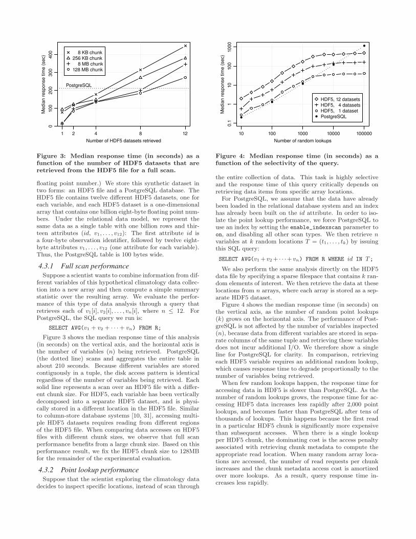
Figure 4: Median response time (in seconds) as afunction of the selectivity of the query.

the entire collection of data. This task is highly selectiveand the response time of this query critically depends onretrieving data items from specific array locations.

For PostgreSQL, we assume that the data have alreadybeen loaded in the relational database system and an indexhas already been built on the id attribute. In order to iso-late the point lookup performance, we force PostgreSQL touse an index by setting the enable_indexscan parameter toon, and disabling all other scan types. We then retrieve n

variables at k random locations T = (t1, . . . , tk) by issuingthis SQL query:

SELECT AVG(v1+ v2+ · · ·+ vn) FROM R WHERE id IN T;

We also perform the same analysis directly on the HDF5data file by specifying a sparse filespace that contains k ran-dom elements of interest. We then retrieve the data at theselocations from n arrays, where each array is stored as a sep-arate HDF5 dataset.

Figure 4 shows the median response time (in seconds) onthe vertical axis, as the number of random point lookups(k) grows on the horizontal axis. The performance of Post-greSQL is not affected by the number of variables inspected(n), because data from different variables are stored in sepa-rate columns of the same tuple and retrieving these variablesdoes not incur additional I/O. We therefore show a singleline for PostgreSQL for clarity. In comparison, retrievingeach HDF5 variable requires an additional random lookup,which causes response time to degrade proportionally to thenumber of variables being retrieved.

When few random lookups happen, the response time foraccessing data in HDF5 is slower than PostgreSQL. As thenumber of random lookups grows, the response time for ac-cessing HDF5 data increases less rapidly after 2,000 pointlookups, and becomes faster than PostgreSQL after tens ofthousands of lookups. This happens because the first readin a particular HDF5 chunk is significantly more expensivethan subsequent accesses. When there is a single lookupper HDF5 chunk, the dominating cost is the access penaltyassociated with retrieving chunk metadata to compute theappropriate read location. When many random array loca-tions are accessed, the number of read requests per chunkincreases and the chunk metadata access cost is amortizedover more lookups. As a result, query response time in-creases less rapidly.

Table Cardinality Columnscandidate 672,912,156 48

rb_classifier 672,906,737 9subtraction 1,039,758 51

Table 1: Our snapshot of the PTF database.

Matching Tuples inσs time subtraction Cardinality

Query interval that match σs of the resultQ1 hour 226 5,878Q2 night 2,876 42,530Q3 week 21,026 339,634

Table 2: Number of tuples that match the filtercondition, and cardinalities of the final answers.

4.3.3 Summary of results from the synthetic dataset

We find that the performance of a sequential data scanwith the HDF5 library is comparable to the performance ofPostgreSQL, if the HDF5 chunk size is hundreds of megabytes.A full scan over a single HDF5 dataset can be significantlyfaster because of the vertically-partitioned nature of theHDF5 file format. Performance drops when multiple HDF5datasets are retrieved, because these accesses will be scat-tered within the HDF5 file. When comparing the pointlookup performance of the HDF5 library with PostgreSQL,we find that accessing individual elements from multipleHDF5 datasets can be one order of magnitude slower thanone B-tree lookup in PostgreSQL, because the HDF5 ac-cesses have no locality.

4.4 Evaluating the SDS/Q prototype using thePalomar Transient Factory workload

The Palomar Transient Factory is an automated survey ofthe sky for transient astronomical events, such as super-novae. Over the past 15 years, observations of supernovaehave been the basis for scientific breakthroughs such as theaccelerating universe [28]. Because the phenomena are tran-sient, a critical component of the survey is the automatedtransient detection pipeline that enables the early detectionof these events. A delay of a few hours in the data process-ing pipeline may mean that astronomers will need to waitfor the next night to observe an event of interest.

The data processing pipeline starts on the site of the wide-field survey camera. The first step is image subtraction,where event candidates are isolated and extracted. The can-didates are then classified through a complex machine learn-ing pipeline [9] which detects whether the candidate is real oran image artifact, and if it is real, what is the transient typeof the candidate (supernova, variable star, etc.). After thisinitial processing, each candidate event is described with 47different variables, and each image subtraction with 50 vari-ables. The classifier has produced a list of matches betweencandidate events and image subtractions (an M-to-N rela-tionship) and 7 generated variables containing confidencescores about each match.

The data are then loaded into a PostgreSQL database forprocessing. The database schema consists of three tables.The candidate table contains one row for each candidateevent, the subtraction table contains one row for each im-age subtraction, and the rb_classifier table has one rowper potential match between a candidate event and an image

subtraction candidate

rb_classifier

σs σc

σr

✶

✶

(a) PTF query plan.

Q1 Q2 Q3

02

00

40

06

00

80

0

Me

dia

n r

esp

on

se

tim

e (

se

c)

45

2

46

9

46

8

56

9

578 6

30

PostgreSQL

SDS/Q

(b) Query response time.

Figure 5: Query performance for the three PTFqueries when performing a full scan.

subtraction. Every variable is stored as a separate column,and an id field is prepended to differentiate each observationand combine information through joins between the tables.We have obtained a nightly snapshot of the database usedby the PTF team for near-real-time transient event detec-tion for evaluating our SDS/Q prototype. The snapshot weexperiment with is a PostgreSQL database of about 180GBof raw data, with another 200GB of space used by indexesto speed up query processing. The cardinalities of the threetables, and the size of each tuple are shown in Table 1.

The workhorse query for this detection workload is a three-way join. The query seeks to find events in the candi-

date table exceeding certain size and brightness thresholds,that have been observed in images in the subtraction tableover some time interval of interest, and are high-confidencematches (based on the scores in the rb_classifier table.)The final result returns 18 columns for further processingand visualization by scripts written by the domain experts.PostgreSQL evaluates this query using the query plan shownin Figure 5(a). By varying the time interval of interest,we create three queries with different selectivities from thisquery template. Each query corresponds to three differentscientific use cases. Q1 looks for matches over the time spanof one hour and is extremely selective, as it returns only0.02% of the tuples in the subtraction table. This is an ex-ample of a near-real-time query that runs periodically duringthe night. Q2 matches an entire night of observations, andreturns 0.3% of the tuples in the subtraction table. Finally,Q3 is looking for matches over last week’s image archive.The selectivity of the condition on the subtraction table isabout 2%. Table 2 shows how many tuples match the filtercondition, and the cardinality of the answer.

4.4.1 Query performance without indexing

If an index has not been constructed yet, PostgreSQL eval-uates all PTF queries by scanning the entire input relations,and uses the hash join as the join algorithm of choice. Weexecute the same query plan in SDS/Q to evaluate the per-formance of in situ data processing in the HDF5 file format.

Figure 5(b) shows the median response time (in seconds)on the vertical axis for each of the three queries. We find thatthe response time of SDS/Q is similar to that of PostgreSQLfor all three queries, and SDS/Q completes all queries about

1 2 4 8 16 32 64 128 256 512

012

02

40

36

04

80

60

0

Re

sp

on

se

tim

e (

se

c)

Number of requested processors

PostgreSQL

SDS/Q

Hive

1801 926

Figure 6: PTF Q1 response time as more processorsare requested from the job scheduler.

25% faster. SDS/Q outperforms PostgreSQL because thequery retrieves HDF5 datasets selectively from each table,as only about 10 out of the approximately 50 attributes ofthe candidate and rb_classifier table are accessed. (Wehave systematically explored this effect in Section 4.3.1.)The performance improvement for SDS/Q is because of thevertically-partitioned layout of the HDF5 datasets that re-sults in less I/O for the three PTF queries.

4.4.2 Parallel processing of native HDF5 data

All experiments so far have presented single-threaded per-formance. A major advantage of native scientific data for-mats such as HDF5 is that they have been designed for par-allel processing on modern supercomputers. In this section,we evaluate how the response time for PTF Q1 improves(on the same data) if one requests more than one processingcore when the batch job is submitted for execution.

Figure 6 shows the response time of the PTF Q1 queryas more processors are requested when the job is submit-ted for execution. We request n cores to be allocated on⌈n8⌉ compute nodes. PostgreSQL has not been designed for

a parallel computing environment, therefore we only showresponse time for a single core. We instead compare theperformance of SDS/Q with the Apache Hadoop data pro-cessing stack. As the PTF queries generate small interme-diate results (cf. Table 2), we have rewritten the query toforce each join to use the efficient map-only broadcast join,instead of the expensive repartition join [8]. Analyzing thePTF dataset with Hive using 8 processors (one node) takes30 minutes, but performance improves almost proportion-ally with the number of processors: the analysis takes lessthan two minutes when using 256 cores. The poor perfor-mance of Hive is rooted in the fact that the Apache Hadoopstack has not been designed for a high-performance environ-ment like the Carver supercomputer, where the parallel filesystem can offer up to 80GB/sec of disk read throughput.As indicated by the near-optimal speedup when allocatingmore processors, the Hive query is a CPU-bound task in thisenvironment.

SDS/Q parallelizes the PTF Q1 query to use all n coresautomatically in the HDF5 scan operator (see Algorithm 1),and uses the broadcast hash join to create identical hashtables in every node to compute the join result. The perfor-mance of SDS/Q improves significantly from parallel data

Q1 Q2 Q3 Q1 Q2 Q3

First query Subsequent queries

010

20

30

40

Me

dia

n r

esp

on

se

tim

e (

se

c)

3.5

5

5.6

2

13

.51

0.2

6

1.8

4

7.18

6.2

3

3.6

1

5.6

9 9.0

5

34

.19

0.1

2

1.9

2

27.

53

93 360 79 358

PostgreSQL SDS/Q pos. index SDS/Q FastBit

Figure 7: Median response time of the three PTFqueries when accessing data through an index.

processing, and when using 16 cores (two nodes) the re-sponse time drops to less than one minute. There are lim-ited performance improvements when using more than 64cores. This is caused by two factors. First, there are highfixed overheads to initiate a new job. Given the small sizeof the original database, these fixed overheads become sig-nificant very quickly at scale. (For example, at 128 coreseach spawned task is processing less than 2GB of data.)The second factor is skew. The references on the candi-

date and rb_classifier tables exhibit high locality for anychosen time range on the subtraction table. This causes afew cores to encounter many matches that propagate acrossthe two joins, while the majority of the processors find nomatches after the first join and terminate quickly. In sum-mary, we find that SDS/Q can significantly improve queryprocessing performance when more processors are requested,and SDS/Q completes the PTF Q1 query 10× – 15× fasterthan Hive on the Carver supercomputer.

4.4.3 Using an index for highly selective queries

We now turn our attention to how indexing can improvethe response time of highly selective queries. PostgreSQLrelies on an index for the range lookup on subtraction, andon index-based joins for the rb_classifier and candidate

tables. We adopt the same query plan for SDS/Q.Figure 7 shows the response time for all PTF queries when

accessing data through an index. We ran a given querymultiple times, in sequence, and report the response time ofthe “cold”first query on the left, and the“warm” subsequentqueries on the right. PostgreSQL relies on a B-tree index,and SDS/Q uses either a positional index (Algorithm 2) orFastBit (Algorithm 3).

Performance is poor for all queries that use the positionalindex. As described in detail in Algorithm 2, this opera-tion consists of two steps: it first retrieves offsets from thepositional index, and then retrieves specific elements fromthe HDF5 file at these offsets. As shown in prior work [3],retrieving the offsets from the positional index is fast. Theperformance bottleneck is retrieving elements at specific off-sets in the HDF5 file, which we have explored systematicallyin Section 4.3.2 (cf. Figure 4). Aside from response time,another important consideration is the amount of workingmemory that a join requires [7]. The FastBit index semi-joinand positional map join have different memory footprints.

SystemTime (minutes)Load Index

PostgreSQL 212.4 99.6SDS/Q 0 11.3

Hive 0 N/A

Table 3: Data preparation time (in minutes) ofdifferent systems for the PTF database.

As FastBit is forming an intermediate result table, it may ac-cess a number of different bitmap indexes for each retrievedvariable, which requires more working memory. Therefore,positional indexing may still be appropriate when the avail-able working memory is limited.

Both PostgreSQL and SDS/Q with FastBit return resultsnearly instantaneously for the most selective PTF query(Q1). As the query becomes less selective (Q3), the queryresponse time from SDS/Q is 3.8× faster than PostgreSQL.PostgreSQL benefits from high selectivity as it stores eachtuple contiguously: all variables can be retrieved with onlyone I/O request. In comparison, SDS/Q relies on FastBitfor both indexing and data access. FastBit partitions datavertically during indexing, hence SDS/Q needs to performmultiple I/O requests to retrieve all data. As the querybecomes less selective, SDS/Q can identify all matching tu-ples at once from the bitmap indexes on rb_classifier andcandidate (see Algorithm 3). In comparison, PostgreSQLhas to perform multiple B-tree traversals to retrieve all data.

To summarize, we find that SDS/Q with FastBit bitmapindexing delivers performance that is comparable to that ofPostgreSQL for extremely selective queries. As the queriesbecome less selective, the bitmap index favors SDS/Q, whereit outperforms PostgreSQL by nearly 4×. Positional index-ing performs poorly due to the inherent cost of performingrandom point lookups over HDF5 data.

4.4.4 The user perspective: end-to-end time

The user of a scientific data analysis system wants to un-derstand the data produced by some simulation or observedduring an experiment. For the case of the PTF dataset, theastronomer has the choice of loading the data in a relationaldatabase system, which takes significant time (see Table 3).Alternatively the astronomer can choose to process the datain situ using SDS/Q or Hadoop [12], leaving data in a fileformat that is understood by the analysis scripts and visu-alization tools she is using already.

Figure 8 shows the time it takes for the astronomer togain the desired insight from the PTF database on the ver-tical axis, as a function of the number of Q1 queries thatneed to be completed on the horizontal axis. Using fourCarver compute nodes, the scientist can get an answer toher first question in about 30 seconds by running SDS/Q onall processing cores. In comparison, the first answer fromHive needs approximately eight minutes. PostgreSQL wouldrespond after the time-consuming data load process is com-plete, which takes four hours. If the scientist desires to askmultiple questions over the same dataset, the indexing ca-pabilities of SDS/Q can produce the final answer faster thanloading and indexing the data in PostgreSQL, or perform-ing full scans in parallel. Due to the cumbersome data loadprocess of the PTF database, the sophisticated querying ca-pabilities of a relational database only outperform SDS/Qafter many thousands of queries. SDS/Q allows scientists

1 10 100 1 K 10 K 100 K 1 M

30 secs

2 mins

10 mins

1 hr

4 hrs

24 hrs

Tim

e to

in

sig

ht

Number of PTF Q1 queries until insight

PostgreSQL, B−tree index, 1 core

PostgreSQL, scan, 1 core

SDS/Q, FastBit index, 1 core

Hive, scan, 32 cores

SDS/Q, scan, 32 cores

Figure 8: Time to insight as a function of the num-ber of the PTF Q1 queries completed. The result forthe first query includes the data preparation time.

to take advantage of the ample parallelism of a supercom-puter through a parallel relational query processing engineand a fast bitmap index without modifying their existingdata analysis workflow.

5. CONCLUSIONSWe propose an in situ relational parallel query processingsystem that operates directly on the popular HDF5 scien-tific file format. This prototype system, named SDS/Q,provides a relational query interface that directly accessesdata stored in the HDF5 format without first loading thedata. By removing the need to convert and load the dataprior to querying, we are able to answer the first query ofthe Palomar Transient Factory (PTF) cosmology workloadmore than 40× faster than loading and querying the rela-tional database system that the scientists use today.

In addition, SDS/Q is able to easily take advantage ofthe parallelism available in a supercomputing system andeffortlessly speed up query processing by simply requestingmore CPU cores when the batch job is submitted for exe-cution. Given that parallel database systems are often tooexpensive for large scientific applications, this ease of par-allelization is an important feature of SDS/Q for processingscientific data. In a test with the same query from the PTFcosmology dataset, SDS/Q responds 10× faster than ApacheHive when running on 512 CPU cores.

We also demonstrate that SDS/Q can use bitmap indexesto significantly reduce query response times. The bitmapindexes are external indexes and do not alter the base datastored in the HDF5 files. On sample queries from the samePTF workload, these bitmap indexes are able to reduce thequery processing time from hundreds of seconds to a fewseconds or less.

We plan to focus our future work in reducing the time togenerate the bitmap indexes. In the current prototype, thebitmap indexes are built with intermediate data files whichare generated from the HDF5 data. We are working to ac-celerate the index build phase by directly reading data fromthe HDF5 file. This will reduce the time needed to answerthe first query using a bitmap index. We also plan to extend

our Scientific Data Services to support operations that areimportant to scientific applications that manipulate largescientific datasets, such as transparent transposition, andreorganization based on query patterns. Finally, query op-timization on shared-disk supercomputers has unique chal-lenges and opportunities, and we see this as a promisingavenue for future work.

Source code

The source code for the core SDS/Q components is available:• Bitmap index: https://sdm.lbl.gov/fastbit/• Query engine: https://github.com/sblanas/pythia/

Acknowledgements

We would like to acknowledge the insightful comments andsuggestions of three anonymous reviewers that greatly im-proved this paper. In addition, we thank Avrilia Floratouand Yushu Yao for assisting with the Hive setup, and PeterNugent for answering questions about the PTF workload.This work was supported in part by the Director, Office ofLaboratory Policy and Infrastructure Management of theU.S. Department of Energy under Contract No. DE-AC02-05CH11231, and used resources of The National Energy Re-search Scientific Computing Center (NERSC).

6. REFERENCES

[1] NetCDF. http://www.unidata.ucar.edu/software/netcdf.[2] The HDF5 Format. http://www.hdfgroup.org/HDF5/.[3] I. Alagiannis, R. Borovica, M. Branco, S. Idreos, and

A. Ailamaki. NoDB: Efficient query execution on raw datafiles. In SIGMOD, pages 241–252, 2012.

[4] C. Balkesen, G. Alonso, J. Teubner, and M. T. Ozsu.Multi-core, main-memory joins: Sort vs. hash revisited.PVLDB, 7(1):85–96, 2013.

[5] P. Baumann, A. Dehmel, P. Furtado, R. Ritsch, andN. Widmann. The multidimensional database systemRasDaMan. In ACM SIGMOD, 1998.

[6] B. Behzad, H. V. T. Luu, J. Huchette, et al. Tamingparallel I/O complexity with auto-tuning. In SC, 2013.

[7] S. Blanas and J. M. Patel. Memory footprint matters:efficient equi-join algorithms for main memory dataprocessing. In SoCC, 2013.

[8] S. Blanas, J. M. Patel, V. Ercegovac, J. Rao, E. J. Shekita,and Y. Tian. A comparison of join algorithms for logprocessing in MapReduce. In ACM SIGMOD, 2010.

[9] J. S. Bloom, J. W. Richards, P. E. Nugent, et al.Automating discovery and classification of transients andvariable stars in the synoptic survey era. arXiv preprintarXiv:1106.5491, 2011.

[10] P. A. Boncz, M. Zukowski, and N. Nes. MonetDB/X100:Hyper-pipelining query execution. In CIDR, 2005.

[11] P. G. Brown. Overview of SciDB: Large scale array storage,processing and analysis. In ACM SIGMOD, 2010.

[12] J. B. Buck, N. Watkins, J. LeFevre, K. Ioannidou,C. Maltzahn, N. Polyzotis, and S. A. Brandt. SciHadoop:array-based query processing in Hadoop. In SC, 2011.

[13] G. Candea, N. Polyzotis, and R. Vingralek. A scalable,predictable join operator for highly concurrent datawarehouses. PVLDB, 2(1):277–288, 2009.

[14] C.-Y. Chan and Y. E. Ioannidis. Bitmap index design andevaluation. In SIGMOD, 1998.

[15] C. Y. Chan and Y. E. Ioannidis. An efficient bitmapencoding scheme for selection queries. In SIGMOD, 1999.

[16] Y. Cheng, C. Qin, and F. Rusu. GLADE: Big dataanalytics made easy. In SIGMOD, pages 697–700, 2012.

[17] J. Chou, K. Wu, and Prabhat. FastQuery: A generalindexing and querying system for scientific data. InSSDBM, pages 573–574, 2011.

[18] B. Dong, S. Byna, and K. Wu. SDS: A framework forscientific data services. In Proceedings of the 8th ParallelData Storage Workshop, PDSW ’13, pages 27–32, 2013.

[19] G. Graefe. Encapsulation of parallelism in the Volcanoquery processing system. In SIGMOD, pages 102–111, 1990.

[20] W. Gropp, E. Lusk, N. Doss, and A. Skjellum. Ahigh-performance, portable implementation of the MPImessage passing interface standard. Parallel Comput.,22(6):789–828, Sept. 1996.

[21] S. Idreos, F. Groffen, N. Nes, et al. MonetDB: Two decadesof research in column-oriented database architectures.IEEE Data Eng. Bull., 35(1):40–45, 2012.

[22] IPCC 2013. Climate Change 2013: The Physical ScienceBasis. Contribution of Working Group I to the FifthAssessment Report of the Intergovernmental Panel onClimate Change. Cambridge University Press, in press.

[23] S. Lakshminarasimhan, D. A. Boyuka, et al. Scalable insitu scientific data encoding for analytical query processing.In HPDC, pages 1–12, 2013.

[24] L. Libkin, R. Machlin, and L. Wong. A query language formultidimensional arrays: Design, implementation, andoptimization techniques. In SIGMOD, 1996.

[25] A. P. Marathe and K. Salem. Query processing techniquesfor arrays. The VLDB Journal, 11(1):68–91, Aug. 2002.

[26] E. Ogasawara, D. Jonas, et al. Chiron: A parallel engine foralgebraic scientific workflows. Journal of Concurrency andComputation: Practice and Experience, 25(16), 2013.

[27] P. E. O’Neil. Model 204 architecture and performance. InHPTS, pages 40–59, 1989.

[28] S. Perlmutter. Nobel Lecture: Measuring the accelerationof the cosmic expansion using supernovae. Reviews ofModern Physics, 84:1127–1149, July 2012.

[29] A. Shoshani and D. Rotem, editors. Scientific DataManagement: Challenges, Technology, and Deployment.Chapman & Hall/CRC Press, 2009.

[30] E. Soroush, M. Balazinska, and D. Wang. ArrayStore: Astorage manager for complex parallel array processing. InACM SIGMOD, pages 253–264, 2011.

[31] M. Stonebraker, D. J. Abadi, A. Batkin, et al. C-store: Acolumn-oriented DBMS. In VLDB, pages 553–564, 2005.

[32] Y. Su and G. Agrawal. Supporting user-defined subsettingand aggregation over parallel NetCDF datasets. InIEEE/ACM CCGRID, pages 212–219, 2012.

[33] R. Thakur, W. Gropp, and E. Lusk. On implementingMPI-IO portably and with high performance. In IOPADS,pages 23–32, 1999.

[34] A. R. van Ballegooij. RAM: A multidimensional arrayDBMS. In EDBT, pages 154–165, 2004.

[35] Y. Wang, W. Jiang, and G. Agrawal. SciMATE: A novelMapReduce-like framework for multiple scientific dataformats. In CCGRID, pages 443–450, 2012.

[36] Y. Wang, Y. Su, and G. Agrawal. Supporting a light-weightdata management layer over HDF5. In CCGRID, 2013.

[37] K. Wu. FastBit: An efficient indexing technology foraccelerating data-intensive science. Journal of Physics:Conference Series, 16:556–560, 2005.

[38] K. Wu, E. Otoo, and A. Shoshani. Optimizing bitmapindices with efficient compression. ACM Transactions onDatabase Systems, 31:1–38, 2006.

[39] Y. Zhang, M. Kersten, and S. Manegold. SciQL: Array dataprocessing inside an RDBMS. In ACM SIGMOD, 2013.

[40] H. Zou, M. Slawinska, K. Schwan, et al. FlexQuery: Anonline in-situ query system for interactive remote visualdata exploration at large scale. In IEEE Cluster, 2013.