Parallel Algorithm Design

Parallel Algorithm Design• Look at Ian Foster’s Methodology (PCAM)• Partition

– Decompose the problem– Identify the concurrent tasks– Often the most difficult step

• Communication– Often dictated by partition

• Agglomeration– Often not much you can do here

• Mapping– Difficult problem– Load Balancing

We will focus on Partitioning and MappingWe will focus on Partitioning and Mapping

Preliminaries

• A given problem may be partitioned in many different ways.

• Tasks may be the same, different, or even indeterminate sizes– Coarse grain – large tasks– Fine grain – very small tasks

• Often, partitionings are illustrated in the form of a “task dependency graph”– Directed graph – Nodes are tasks– Edges denote that the result of one task is

needed for the computation of the result in another task

Task Dependency Graph

• Can be a graph or adjacency matrix

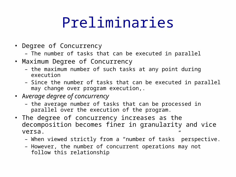
Preliminaries• Degree of Concurrency

– The number of tasks that can be executed in parallel

• Maximum Degree of Concurrency– the maximum number of such tasks at any point during

execution– Since the number of tasks that can be executed in parallel may

change over program execution,.

• Average degree of concurrency – the average number of tasks that can be processed in parallel

over the execution of the program.

• The degree of concurrency increases as the decomposition becomes finer in granularity and vice versa.– When viewed strictly from a “number of tasks” perspective.– However, the number of concurrent operations may not follow

this relationship

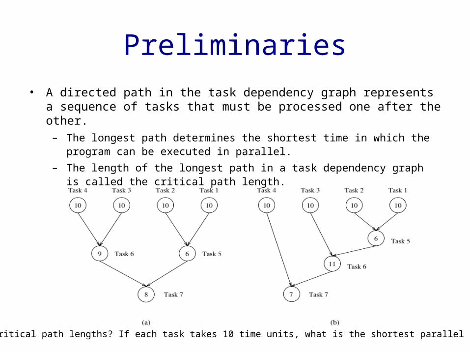
Preliminaries• A directed path in the task dependency graph represents a

sequence of tasks that must be processed one after the other. – The longest path determines the shortest time in which the program

can be executed in parallel.

– The length of the longest path in a task dependency graph is called the critical path length.

What are the critical path lengths? If each task takes 10 time units, what is the shortest parallel execution time?

Limits on Parallel Performance

• It would appear that the parallel time can be made arbitrarily small by making the decomposition finer in granularity.

• There is an inherent bound on how fine the granularity of a computation can be. – For example, in the case of multiplying a dense matrix

with a vector, there can be no more than (n2) concurrent tasks.

• Concurrent tasks may also have to exchange data with other tasks. This results in communication overhead.

• The tradeoff between the granularity of a decomposition and associated overheads often determines performance bounds.

Partitioning Techniques

• There is no single recipe that works for all problems.

• We can benefit from some commonly used techniques:– Recursive Decomposition– Data Decomposition– Exploratory Decomposition– Speculative Decomposition

Recursive Decomposition

• Generally suited to problems that are solved using a divide and conquer strategy.

• Decompose based on sub-problems• Often results in natural concurrency as

sub-problems can be solved in parallel.

• Need to think recursively– parallel not sequential

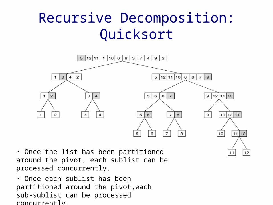
Recursive Decomposition: Quicksort

• Once the list has been partitioned around the pivot, each sublist can be processed concurrently. • Once each sublist has been partitioned around the pivot,each sub-sublist can be processed concurrently.• Once each sub-sublist …

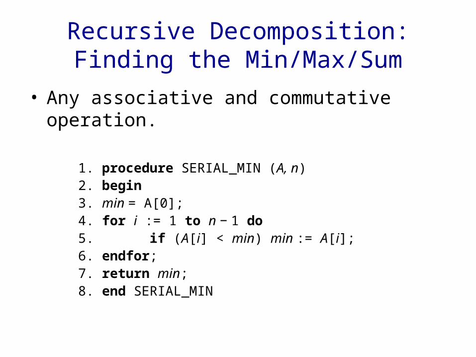
Recursive Decomposition:Finding the Min/Max/Sum

• Any associative and commutative operation.

1. procedure SERIAL_MIN (A, n)2. begin3. min = A[0];4. for i := 1 to n − 1 do5. if (A[i] < min) min := A[i];6. endfor;7. return min;8. end SERIAL_MIN

Recursive Decomposition:Finding the Min/Max/Sum

• Rewrite using recursion and max partitioning– Don’t make a serial recursive routine

1. procedure RECURSIVE_MIN (A, n) 2. begin 3. if ( n = 1 ) then 4. min := A [0] ; 5. else 6. lmin := RECURSIVE_MIN ( A, n/2 ); 7. rmin := RECURSIVE_MIN ( &(A[n/2]), n - n/2 ); 8. if (lmin < rmin) then 9. min := lmin; 10. else 11. min := rmin; 12. endelse; 13. endelse; 14. return min; 15. end RECURSIVE_MIN

Note: Divide the workin half each time.Note: Divide the workin half each time.

Recursive Decomposition:Finding the Min/Max/Sum

• Example: Find min of {4,9,1,7,8,11,2,12}

4 9 1 7 8 11 2 12

1 9 1 7 2 11 2 12

1 9 1 7 2 11 2 12

Step

1

2

3

Recursive Decomposition:Finding the Min/Max/Sum

• Strive to divide in half• Often, can be mapped to a

hypercube for a very efficient algorithm

• Make sure that the overhead of dividing the computation is worth it.– How much does it cost to communicate

necessary dependencies?

Data Decomposition

• Most common approach• Identify the data and partition across

tasks• Can partition in various ways

– critically impacts performance• Three approaches

– Output Data Decomposition– Input Data Decomposition– Domain Decomposition

Output Data Decomposition

• Often, each element of the output can be computed independently of the others– A function of the input– All may be able to share the input or have a

copy of their own

• Often decomposes the problem naturally.

• Embarrassingly Parallel– Output data decomposition with no need for

communication– Mandelbrot, Simple Ray Tracing, etc.

Output Data Decomposition

• Matrix Multiplication: A * B = C• Can partition output matrix C

Output Data Decomposition

• Count the instances of given itemsets

Input Data Decomposition

• Applicable if the output can be naturally computed as a function of the input.

• In many cases, this is the only natural decomposition because the output is not clearly known a-priori– finding minimum in list, sorting, etc.

• Associate a task with each input data partition.

• Tasks communicate where necessary input is “owned” by another task.

Input Data Decomposition

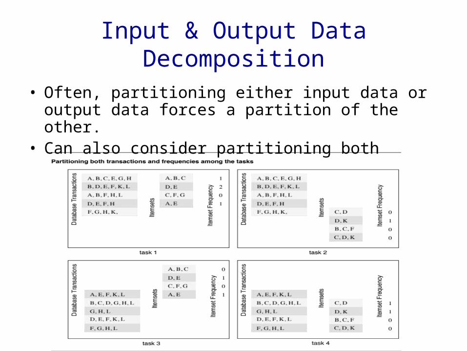
• Count the instances of given itemsets• Each task generates partial counts for all

itemsets which must be aggregated.

• Must combine partial results at the end

Input & Output Data Decomposition

• Often, partitioning either input data or output data forces a partition of the other.

• Can also consider partitioning both

Domain Decomposition

• Often can be viewed as input data decomposition– May not be input data– Just domain of calculation

• Split up the domain among tasks• Each task is responsible for computing

the answer for its partition of the domain

• Tasks may end up needing to communicate boundary values to perform necessary calculations

Domain Decomposition

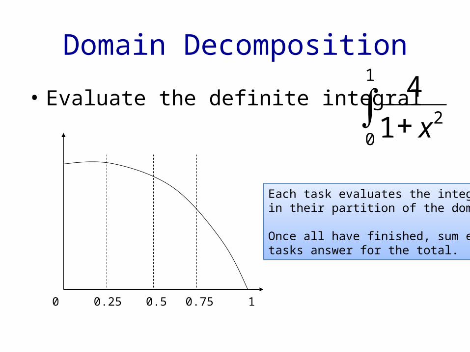
• Evaluate the definite integral

1

021

4

x

0 10.50.25 0.75

Each task evaluates the integralin their partition of the domain

Once all have finished, sum eachtasks answer for the total.

Each task evaluates the integralin their partition of the domain

Once all have finished, sum eachtasks answer for the total.

Domain Decomposition

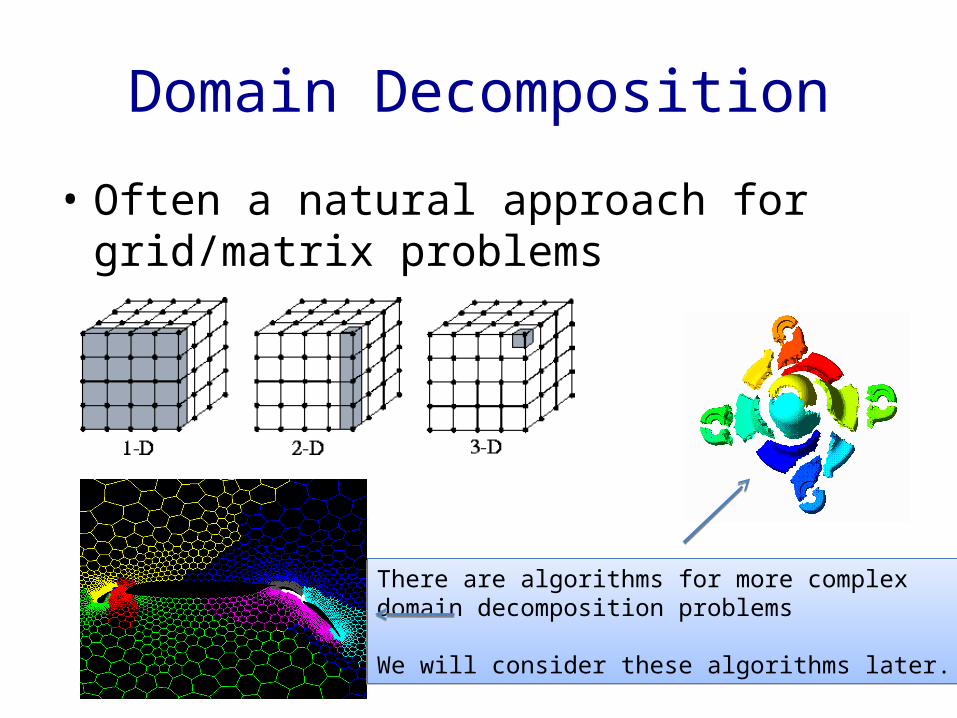
• Often a natural approach for grid/matrix problems

There are algorithms for more complexdomain decomposition problems

We will consider these algorithms later.

There are algorithms for more complexdomain decomposition problems

We will consider these algorithms later.

Exploratory Decomposition

• In many cases, the decomposition of a problem goes hand-in-hand with its execution.

• Typically, these problems involve the exploration of a state space.– Discrete optimization– Theorem proving– Game playing

Exploratory Decomposition

• 15 puzzle – put the numbers in order– only move one piece at a time to a blank

spot

Exploratory Decomposition

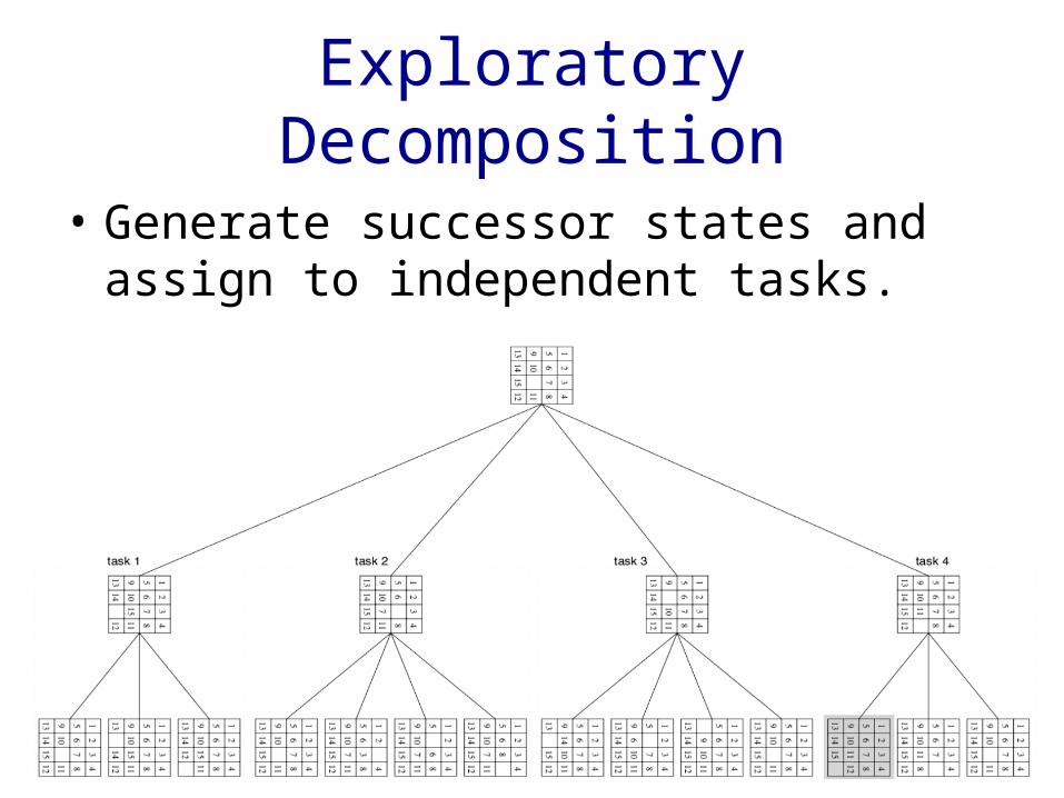
• Generate successor states and assign to independent tasks.

Exploratory Decomposition• Exploratory decomposition techniques may

change the amount of work done by the parallel implementation.

• Change can result in super- or sub-linear speedups

Speculative Decomposition

• Sometimes, dependencies are not known a-priori• Two approaches

– conservative – identify independent tasks only when they are guaranteed to not have dependencies

• May yield little concurrency– optimistic – schedule tasks even when they may be

erroneous• May require a roll-back mechanism in the case of an error.

• The speedup due to speculative decomposition can add up if there are multiple speculative stages

• Examples– Concurrently evaluating all branches of a C switch stmt– Discrete event simulation

Speculative DecompositionDiscrete Event Simulation

• The central data structure is a time-ordered event list. • Events are extracted precisely in time order, processed,

and if required, resulting events are inserted back into the event list.

• Consider your day today as a discrete event system - – you get up, get ready, drive to work, work, eat lunch,

work some more, drive back, eat dinner, and sleep. • Each of these events may be processed independently,

– however, in driving to work, you might meet with an unfortunate accident and not get to work at all.

• Therefore, an optimistic scheduling of other events will have to be rolled back.

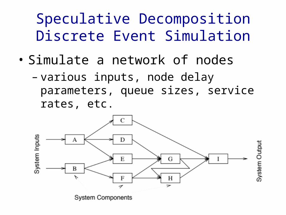
Speculative DecompositionDiscrete Event Simulation

• Simulate a network of nodes– various inputs, node delay parameters,

queue sizes, service rates, etc.

Hybrid Decomposition

• Often, a mix of decomposition techniques is necessary

• In quicksort, recursive decomposition alone limits concurrency (Why?). A mix of data and recursive decompositions is more desirable.

• In discrete event simulation, there might be concurrency in task processing. A mix of speculative decomposition and data decomposition may work well.

• Even for simple problems like finding a minimum of a list of numbers, a mix of data and recursive decomposition works well.

Task Characterization

• Task characteristics can have a dramatic impact on performance

• Task Generation– Static– Dynamic

• Task Size– Uniform– Non-uniform

• Task Data– Size– Uniformity

Task Generation

• Static– known a priori– constant throughout run– image processing, matrix & graph algorithms

• Dynamic– # tasks changes throughout run– difficult to launch during run – scheduled

environment– most often dealt with using dynamic load

balancing techniques

Task Size – Data size

• Execution time– uniform – synchronous steps– non-uniform – difficult to determine

synchronization points• often handled using Master-Worker paradigm• otherwise polling is necessary in message passin

• Data Size– Can determine performance

• swapping• cache effects super-linear speedup

Task Interactions

• Static interactions: The tasks and their interactions are known a-priori. These are relatively simple to code into programs.

• Dynamic interactions: The timing or interacting tasks cannot be determined a-priori. These interactions are harder to code, especially using message passing APIs.

• Regular interactions: There is a definite pattern (in the graph sense) to the interactions. These patterns can be exploited for efficient implementation.

• Irregular interactions: Interactions lack well-defined topologies.

Static Task Interaction PatternsRegular patterns are easier to codeBoth producer and consumer are aware of when communication is required Explicit and Simple code

Regular patterns are easier to codeBoth producer and consumer are aware of when communication is required Explicit and Simple code

Irregular patterns must take intoaccount the variable number of neighbors for each task.Timing becomes more difficult

Irregular patterns must take intoaccount the variable number of neighbors for each task.Timing becomes more difficult

A Sparse Matrix and its associated irregular task interaction graphA Sparse Matrix and its associated irregular task interaction graph

Typical image processing partitioningTypical image processing partitioning

Static & Regular Interaction

• Algorithm has phases of computation and communication

• Example - Hotplate– Communicate initial conditions– Loop

• Communicate dependencies• Calculate “owned” values• Check for convergence in “owned” values• Communicate to determine convergence

– Communicate final conditions

Dynamic Interaction

Tasks don’tknow when toreceive amessage –

periodically poll

Task Interactions

• Read-only or Read-Write– Read-only – just read data items associated with other tasks– Read-write – read and modify data associated with other tasks

• Read-Write interactions are harder to code. They require additional synchronization

• One-way or Two-way– One-way – One task pushes data to another– Two-way – Both tasks are involved

• One-way interactions are not generally available in most message passing APIs

• One-way interactions require either shared memory or support from the system

Mapping

• Once a problem has been decomposed into concurrent tasks, the tasks must be mapped to processes.– Mapping and Decomposition are often interrelated steps

• Mapping must minimize overhead– communication and idling

• Minimizing overhead is a trade-off game– Assigning all work to one processor trivially minimizes

communication at the expense of significant idling.

• Goal: Performance

Mapping

• Load-balancing– NP complete– We will discuss in much more detail later

• Static– tasks mapped to processes a-priori– need a good estimate of the size of each task– often based on data or task graph partitioning

• Dynamic– tasks mapped to processes at runtime.– tasks are either unknown or have indeterminate

processing times

Mapping – Data Partitioning

• Based on “owner-computes” rule

Block-wise distribution

Mapping and Data Sharing

• Partitioning and Mapping often induces the need for communication.

• Changes in mapping schemes can reduce communication needs

• Partitioning and Mapping often create load imbalance due to indeterminate computation times

• Changes in mapping schemes can reduce load imbalance

Data Sharing in Dense Matrix Multiplication

Computation Sharing

• Cyclic distributions often “spread the load”

Mapping

• Irregular interaction graphs are more complex to map

• Goal: Balance the load while minimizing edge-cuts in the task interaction graph– edge-cuts indicate the need for communication

Partitioning Lake Superior for minimum edge-cut.

More on this topic later!More on this topic later!

Dynamic Mapping

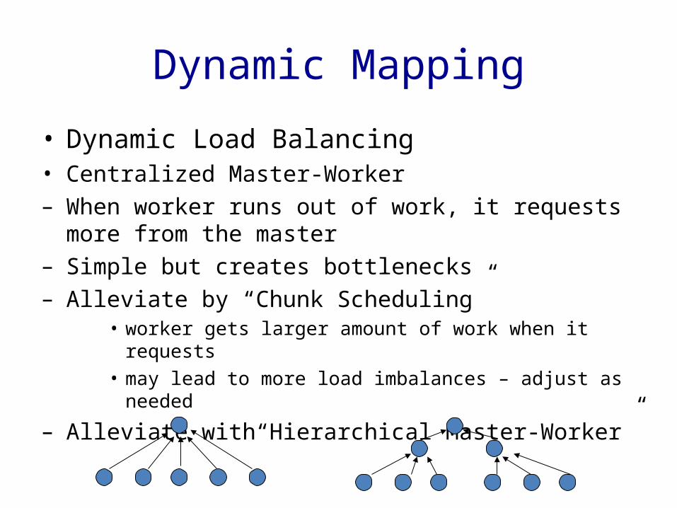
• Dynamic Load Balancing• Centralized Master-Worker– When worker runs out of work, it requests more

from the master– Simple but creates bottlenecks– Alleviate by “Chunk Scheduling”

• worker gets larger amount of work when it requests• may lead to more load imbalances – adjust as needed

– Alleviate with“Hierarchical Master-Worker”

Dynamic Mapping

• Who has the work and where do I get it from when I run out?– Can everybody have it?

• Who initiates work transfer?• How much work is transferred?• How often do we check for load imbalance?• How do we detect load imbalance?

• Often, the answers are application specific.

• More on this topic later!

Minimizing Interaction Overheads

• Maximize data locality– Where possible, reuse intermediate data.– Restructure computation so that data can be reused in

smaller time windows

• Minimize volume of data exchange– There is a cost associated with each word communicated.

• Minimize frequency of interactions– There is a startup cost associated with each interaction– Batch communication if possible

• Minimize contention and hot-spots– Decentralize communication where possible– Replicate data where necessary

Minimizing Interaction Overheads

• Overlap communication with computation– Use non-blocking communication,

multithreading, and prefetching to hide latencies

• Replicate data or computations– It may be less expensive to recalculate or store

redundantly than to communicate

• Use group communication instead of point to point primitives– They are more optimized generally

Example - Hotplate

• Use Domain Decomposition– domain is the hotplate– split the hotplate up among tasks

• row-wise or block-wise

Consider the communication costs

Row-wise 2 neighbors

Block-wise 4 neighbors

Consider the communication costs

Row-wise 2 neighbors

Block-wise 4 neighbors

Consider data sharing and computational needs & efficiency

About the same for row or block

Consider data sharing and computational needs & efficiency

About the same for row or block

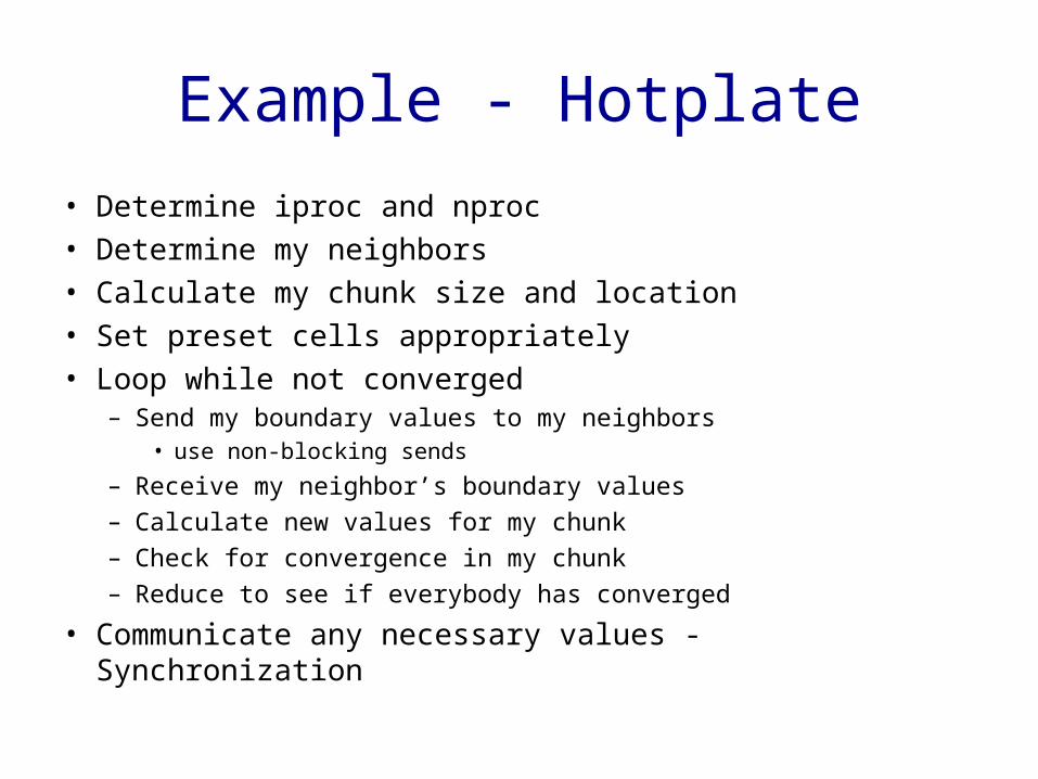
Example - Hotplate

• Determine iproc and nproc• Determine my neighbors• Calculate my chunk size and location• Set preset cells appropriately• Loop while not converged

– Send my boundary values to my neighbors• use non-blocking sends

– Receive my neighbor’s boundary values– Calculate new values for my chunk– Check for convergence in my chunk– Reduce to see if everybody has converged

• Communicate any necessary values - Synchronization

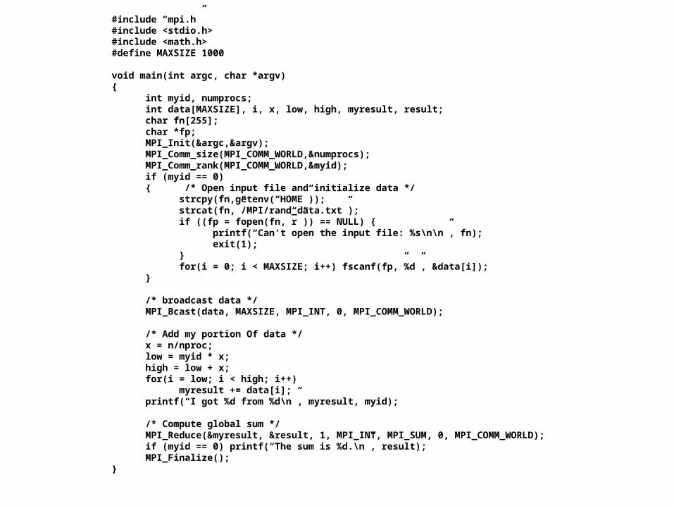
#include “mpi.h”#include <stdio.h>#include <math.h>#define MAXSIZE 1000

void main(int argc, char *argv){

int myid, numprocs;int data[MAXSIZE], i, x, low, high, myresult, result;char fn[255];char *fp;MPI_Init(&argc,&argv);MPI_Comm_size(MPI_COMM_WORLD,&numprocs);MPI_Comm_rank(MPI_COMM_WORLD,&myid);if (myid == 0) { /* Open input file and initialize data */

strcpy(fn,getenv(“HOME”));strcat(fn,”/MPI/rand_data.txt”);if ((fp = fopen(fn,”r”)) == NULL) {

printf(“Can’t open the input file: %s\n\n”, fn);exit(1);

}for(i = 0; i < MAXSIZE; i++) fscanf(fp,”%d”, &data[i]);

}

/* broadcast data */MPI_Bcast(data, MAXSIZE, MPI_INT, 0, MPI_COMM_WORLD);

/* Add my portion Of data */x = n/nproc;low = myid * x;high = low + x;for(i = low; i < high; i++)

myresult += data[i];printf(“I got %d from %d\n”, myresult, myid);

/* Compute global sum */MPI_Reduce(&myresult, &result, 1, MPI_INT, MPI_SUM, 0, MPI_COMM_WORLD);if (myid == 0) printf(“The sum is %d.\n”, result);MPI_Finalize();

}