Chapter �

Transforms

The �rst step in data analysis is to learn how to represent and manipulate waveformsin a digital computer� Time and space are ordinarily regarded as continuous� but forpurposes of computer analysis we must discretize them� This discretizing is also calleddigitizing or sampling� Discretizing continuous functions may at �rst be regarded asan evil that is necessary only because our data are not always known analytic func�tions� However� after gaining some experience with sampled functions� one realizesthat many mathematical concepts are easier with sampled time than with continuoustime� For example� in this chapter� the concept of the Z transform is introducedand is shown to be equivalent to the Fourier transform� The Z transform is readilyunderstood on a basis of elementary algebra� whereas the Fourier transform requiressubstantial experience in calculus�

��� SAMPLED DATA AND Z TRANSFORMS

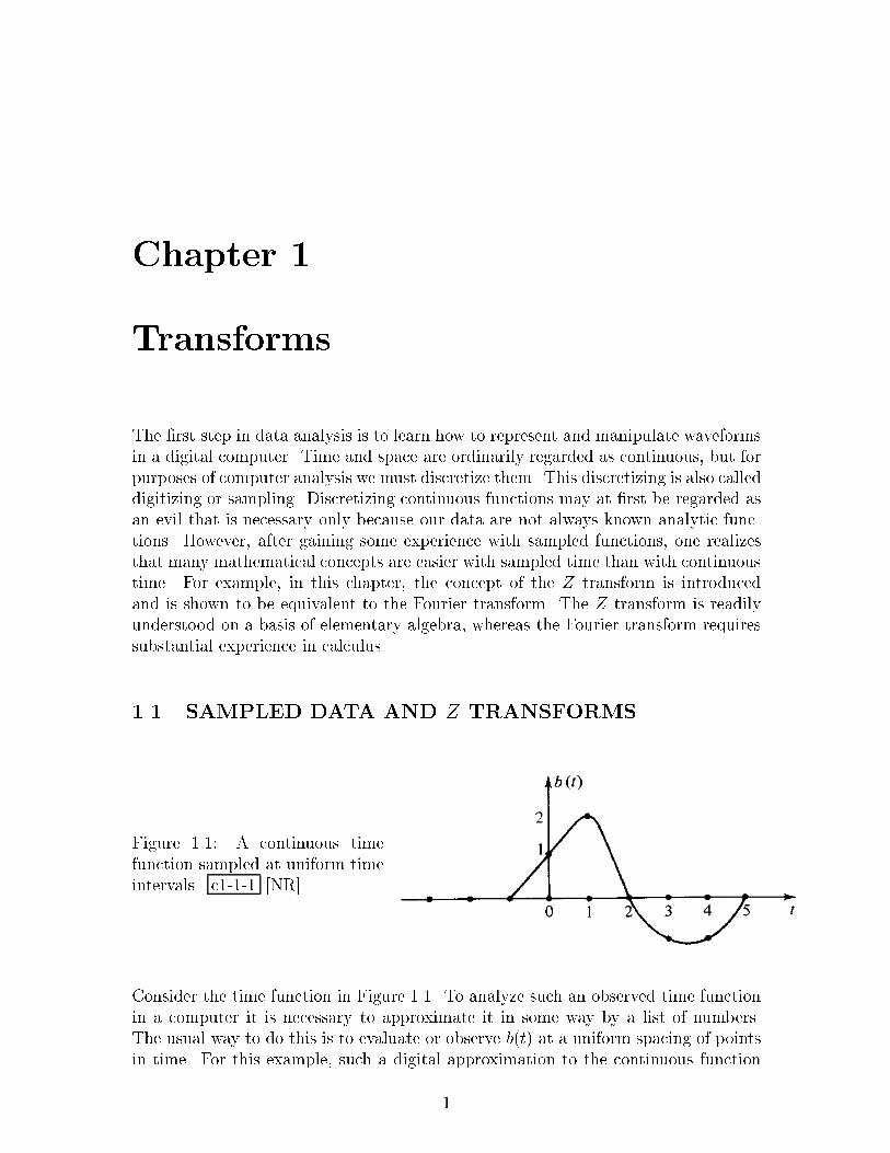
Figure ���� A continuous timefunction sampled at uniform timeintervals� c����� �NR

Consider the time function in Figure ���� To analyze such an observed time functionin a computer it is necessary to approximate it in some way by a list of numbers�The usual way to do this is to evaluate or observe bt� at a uniform spacing of pointsin time� For this example� such a digital approximation to the continuous function

�

� CHAPTER �� TRANSFORMS

could be denoted by the vector

bt � � � �� �� �� �� �� ��� ��� �� �� � � �� ����

Of course if time points were taken more closely together we would have a more accu�rate approximation� Besides a vector� a function can be represented as a polynomialwhere the coe�cients of the polynomial represent the values of bt� at successive timepoints� In this example� we have

BZ� � � �Z � �Z�� Z�

� Z� ����

This polynomial is called a Z transform� What is the meaning of Z in this polynomial�The meaning is not that Z should take on some numerical value� the meaning ofZ is that it is the unit delay operator� For example the coe�cients of ZBZ� Z��Z��Z��Z� are plotted in Figure ���� It is the same waveform as in Figure ����but it has been delayed�

Figure ���� Coe�cients of ZBZ�are shifted version of the coe��cients of BZ� c����� �NR

We see that the time function bt is delayed n time units when BZ� is multipliedby Zn� The delay operator Z is very important in analyzing waves simply becausewaves take a certain amount of time to get from place to place�

Another value of the delay operator is that it may be used to build up morecomplicated time functions from simpler ones� Suppose bt� represents the acousticpressure function or the seismogram observed after a distant explosion� Then bt� iscalled the impulse response� If another explosion occurs at t �� time units afterthe �rst� we expect the pressure function yt� depicted in Figure ����

Figure ���� Response to two ex�plosions� c����� �NR

In terms of Z transforms this would be expressed as Y Z� BZ� � Z��BZ��If the �rst explosion were followed by an implosion of half strength� we would haveBZ�� �

�Z��BZ�� If pulses overlap one another in time �as would be the case if BZ�

���� SAMPLED DATA AND Z TRANSFORMS �

was of degree greater than ��� the waveforms would just add together in the regionof overlap� The supposition that they just add together without any interaction iscalled the linearity assumption� This linearity assumption is very often true in prac�tical cases� In seismology we �nd that�although the earth is a very heterogeneousconglomerations of rocks of di�erent shapes and types�when seismic waves of usualamplitude� travel through the earth� they do not interfere with one another� Theysatisfy linear superposition� The plague of nonlinearity arises from large amplitudedisturbances� Nonlinearity does not arise from geometrical complications�

Now suppose there was an explosion at t �� a half�strength implosion at t ��and another� quarter�strength explosion at t �� This sequence of events determinesa �source� time series� xt ����

�� �� �

��� The Z transform of the source is XZ�

�� ��Z� �

�Z�� The observed yt for this sequence of explosions and implosions through

the seismometer has a Z transform Y Z� given by

Y Z� BZ��Z

�BZ� �

Z�

�BZ�

���

Z

��Z�

�

�BZ�

XZ�BZ� ����

The last equation illustrates the underlying basis of linear�system theory that theoutput Y Z� can be expressed as the input XZ� times the impulse response BZ��

There are many examples of linear systems� A wide class of electronic circuits iscomprised of linear systems� Complicated linear systems are formed by taking theoutput of one system and plugging it into the input of another� Suppose we havetwo linear systems characterized by BZ� and CZ�� respectively� Then the questionarises whether the two combined systems of Figure ��� are equivalent� The use of Ztransforms makes it obvious that these two systems are equivalent since products ofpolynomials commute� i�e��

Y�Z� �XZ�BZ�CZ� XBC

Y�Z� �XZ�CZ�BZ� XCB XBC ����

Consider a system with an impulse response BZ� ��Z�Z�� This polynomialcan be factored into ��Z�Z� ��Z� ��Z�� and so we have the three equivalentsystems in Figure ���� Since any polynomial can be factored� any impulse response canbe simulated by a cascade of two�term �lters impulse responses whose Z transformsare linear in Z��

What do we actually do in a computer when we multiply two Z transforms to�gether� The �lter � � Z would be represented in a computer by the storage inmemory of the coe�cients �� ��� Likewise� for ��Z the numbers ����� are stored�The polynomial multiplication program should take these inputs and produce the

� CHAPTER �� TRANSFORMS

Figure ���� Two equivalent �ltering systems� c����� �NR

Figure ���� Three equivalent �ltering systems� c����� �NR

���� SAMPLED DATA AND Z TRANSFORMS �

sequence ��������� Let us see how the computation proceeds in a general case� say

XZ�BZ� Y Z� ����

x� � x�Z � x�Z � � � �� b� � b�Z � b�Z� y� � y�Z � y�Z� � � � �� ����

Identifying coe�cients of successive powers of Z� we get

y� x�b�

y� x�b� � x�b�

y� x�b� � x�b� � x�b� ����

y� x�b� � x�b� � x�b�

y� x�b� � x�b� � x�b�

yk �X

i��

xk�ibi ����

Equation ���� is called a convolution equation� Thus� we may say that the product oftwo polynomials is another polynomial whose coe�cients are found by convolution�A simple Fortran computer program which does convolution� including end e�ects onboth ends� is this�

DIMENSION X�LX�� B�LB�� Y�LY�

DO �� IY���LY

�� Y�IY� � ��

DO � IX���NX

DO � IB���NB

IY � IXIB��

� Y�IY� � Y�IY� X�IX��B�IB�

The reader should notice that XZ� and Y Z� need not strictly be polynomials�they may contain both positive and negative powers of Z� that is

XZ� � � �x��Z�

�x��Z

� x� � x�Z � � � � ����

Y Z� � � �y��Z�

�y��Z

� y� � y�Z � � � � �����

The e�ect of using negative powers of Z in XZ� and Y Z� is merely to indicate thatdata are de�ned before t �� The e�ect of using negative powers of Z in the �lter isquite di�erent� Inspection of ���� shows that the output yk which occurs at time k isa linear combination of current and previous inputs� that is� xi� i � k�� If the �lterBZ� had included a term like b���Z� then the output yk at time k would be a linearcombination of current and previous inputs and xk��� an input which really has notarrived at time k� Such a �lter is called a nonrealizable �lter because it could notoperate in the real world where nothing can respond now to an excitation which hasnot yet occurred� However� nonrealizable �lters are occasionally useful in computersimulations where all of the data are prerecorded�

� CHAPTER �� TRANSFORMS

EXERCISES�

� Let BZ� � � Z � Z� � Z� � Z�� Graph the coe�cients of BZ� as a functionof the powers of Z� Graph the coe�cients of �BZ���

� If xt cos��t� where t takes on integral values� bt b�� b��� and Y Z� XZ�BZ�� what are A and B in yt A cos��t�B sin��t �

� Deduce that� if xt cos��t and bt b�� b�� � � � � bn�� then yt always takes theform A cos��t �B sin��t�

��� Z�TRANSFORM TO FOURIER TRANSFORM

We have de�ned the Z transform as

BZ� Xt

btZt �����

If we make the substitution Z ei� we have a �Fourier sum�

BZ� Bei�� Xt

btei�t �����

This is like a Fourier integral� and we could do a limiting operation to make it intoan integral� Another point of view is that the Fourier integral

B�� Z ��

��

bt� ei�t dt �����

reduces to the sum ����� when bt� is not a continuous function of time but is de�nedas

bt� Xk

bk �t� k� �����

where � is an impulse function�

In the last section we saw that to multiply two polynomials the coe�cients mustbe convolved� The same process in Fourier transform language is that a product inthe frequency domain corresponds to a convolution in the time domain�

Although one thinks of a Fourier transform as an integral which may be di�cult orimpossible to do� the Z transform is always easy� in fact trivial� To do a Z transformone merely attaches powers of Z to successive data points� When one has BZ� onecan refer to it either as a time function or a frequency function� depending on whetherone graphs the polynomial coe�cients or if one evaluates and graphs BZ ei�� forvarious frequencies �� Notice that as � goes from zero to ��� Z ei� cos�� i sin�migrates once around the unit circle in the counterclockwise direction�

If taking a Z transform amounts to attaching powers of Z to successive points of atime function� then the inverse Z transform must be merely identifying coe�cients of

���� Z�TRANSFORM TO FOURIER TRANSFORM �

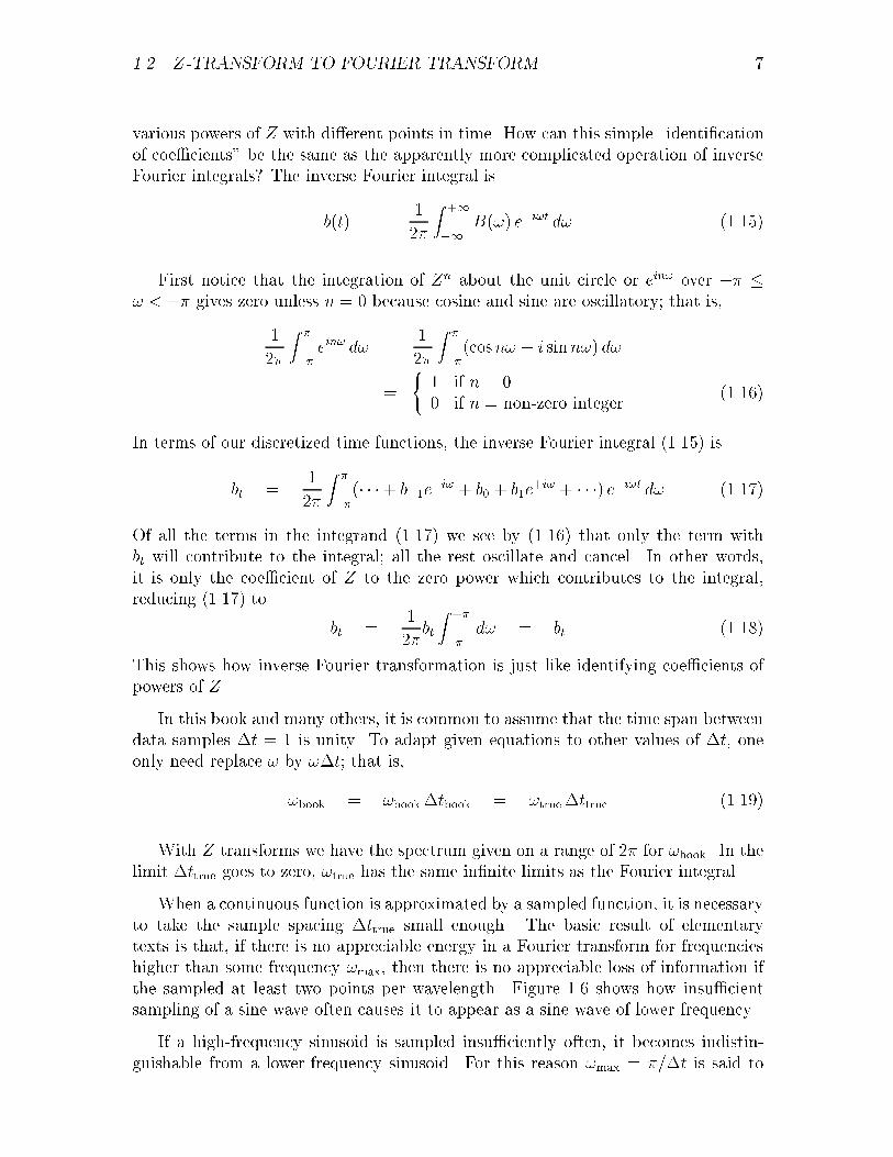
various powers of Z with di�erent points in time� How can this simple �identi�cationof coe�cients� be the same as the apparently more complicated operation of inverseFourier integrals� The inverse Fourier integral is

bt� �

��

Z ��

��

B�� e�i�t d� �����

First notice that the integration of Zn about the unit circle or ein� over �� �

� � �� gives zero unless n � because cosine and sine are oscillatory� that is�

�

��

Z �

��ein� d�

�

��

Z �

��cosn� � i sinn�� d�

�� if n �� if n non�zero integer

�����

In terms of our discretized time functions� the inverse Fourier integral ����� is

bt �

��

Z �

��� � �� b��e

�i� � b� � b�e�i� � � � �� e�i�t d� �����

Of all the terms in the integrand ����� we see by ����� that only the term withbt will contribute to the integral� all the rest oscillate and cancel� In other words�it is only the coe�cient of Z to the zero power which contributes to the integral�reducing ����� to

bt �

��bt

Z ��

��d� bt �����

This shows how inverse Fourier transformation is just like identifying coe�cients ofpowers of Z�

In this book and many others� it is common to assume that the time span betweendata samples �t � is unity� To adapt given equations to other values of �t� oneonly need replace � by ��t� that is�

�book �book�tbook �true�ttrue �����

With Z transforms we have the spectrum given on a range of �� for �book� In thelimit �ttrue goes to zero� �true has the same in�nite limits as the Fourier integral�

When a continuous function is approximated by a sampled function� it is necessaryto take the sample spacing �ttrue small enough� The basic result of elementarytexts is that� if there is no appreciable energy in a Fourier transform for frequencieshigher than some frequency �max� then there is no appreciable loss of information ifthe sampled at least two points per wavelength� Figure ��� shows how insu�cientsampling of a sine wave often causes it to appear as a sine wave of lower frequency�

If a high�frequency sinusoid is sampled insu�ciently often� it becomes indistin�guishable from a lower�frequency sinusoid� For this reason �max ���t is said to

� CHAPTER �� TRANSFORMS

Figure ���� Subsampled sinusoid�c�����a �NR

be the folding frequency� as higher frequencies are folded down to look like lowerfrequencies�

In practice� quasi�sinusoidal waves are always sampled more frequently than twiceper wavelength�

Next we wish to examine odd�even symmetries to see how they are a�ected inFourier transformation� The even part et of a time function bt is de�ned as

et bt � b�t

������

The odd part is

ot bt � b�t

������

A function is the sum of its even and odd parts� By adding ������� and �������� weget

bt et � ot �����

Consider a simple� real� even time function such as b��� b�� b�� �� �� ��� Itstransform Z � ��Z � cos� is an even function of � since cos� cos���� Con�sider the real� odd time function b��� b�� b�� ��� �� ��� Its transform Z � ��Z �sin���i is imaginary and odd� since sin� � sin���� Likewise� the transformof the imaginary even function i� �� i� is the imaginary even function i cos� and thetransform of the imaginary odd function �i� �� i� is real and odd� Let r and i referto real and imaginary� e and o refer to even and odd� and lower�case and upper�case refer to time and frequency functions� A summary of the symmetries of Fouriertransformation is shown in Figure ����

Figure ���� Mnemonic tableillustrating how even�odd andreal�imaginary properties are af�fected by Fourier transformation�c�����b �NR

More elaborate time functions can be made up by adding together the two pointfunctions we have considered� Since sums of even functions are even� and so on� the

���� THE FAST FOURIER TRANSFORM �

table of Figure ��� applies to all time functions� Note that an arbitrary time functiontakes the form bt re � ro�t � iie � io�t� On transformation of bt� each of the fourindividual parts transforms according to the table

EXERCISES�

� Normally a function is speci�ed entirely in the time domain or entirely in the fre�quency domain� When one is known� the other is determined by transformation�Now let us give half the information in the time domain by specifying that bt �for t � �� and half in the frequency domain by giving the real part RE � RO inthe frequency domain� How can you determine the rest of the function�

��� THE FAST FOURIER TRANSFORM

When we write the expression

BZ� b� � b�Z � b�Z� � � � � �����

we have both a time function and its Fourier transform� If we plot the coe�cientsb�� b�� � � ��� we plot the time function� If we evaluate and plot ����� at numerous real�� then we have plotted the transform� Note that for real �� Z is of unit magnitude�i�e�� on the unit circle�� Since � is a continuous variable and everything in a computeris �nite� how do we select a �nite number of values �k for plotting� The usualchoice is to take evenly spaced frequencies� The lowest frequency can be zero� �NoteZ� �� eio �� A frequency as high as � �� �Note Z� ��� ei�� � alsoneed not be considered� since ����� gives the same value for it as for zero frequency�Choosing uniformly spaced frequencies between these limits we have

�k �� �� �� � � � �M � �� ��

M�����

where M is some integer� Now let us abbreviate BZ�k�� as Bk�

For the special case of an N �point time function where N �� ����� may beexpressed by the matrix multiplication

�����B�

B�

B�

B�

����

������ � � �� W W � W �

� W � W � W

� W � W W

���������b�b�b�b�

���� �����

whereW e��i�N �����

It is not essential to choose N M as we have done in ������ but it is a convenience�There is no loss of generality because one may always append zeros to a time function

�� CHAPTER �� TRANSFORMS

before inserting it into ������ A convenience of the choice N M is that the matrixin ����� will then be square and there will be an exact inverse� In fact� the inverseto ����� may be easily shown to be

�����b�b�b�b�

���� ��N

������ � � �� ��W ��W � ��W �

� ��W � ��W � ��W

� ��W � ��W ��W

���������B�

B�

B�

B�

���� �����

Since ��W is the complex conjugate of W � the matrices of ����� and ����� arejust complex conjugates of one another� In fact� one observes no fundamental math�ematical di�erence between time functions and frequency functions� This �duality�would be even more complete if we had used a scale factor of N���� in each of �����and ����� rather than � in ����� and N�� in ������ Note also that time functionsand frequency functions could be interchanged in the mnemonic table describing sym�metries� In fact� our earlier observation that the product of two frequency functionsamounts to a convolution of two time functions corresponds to the convolution of thecorresponding two frequency functions� We will not �provide� this duality as it isstandard fare in both mathematics and systems theory books� However we will occa�sionally call upon the reader to realize that in any theorem the meanings of �time�and �frequency� may be interchanged�

In making a plot of the transform Bk for k �� �� � � � �M � ��� the frequency axisranges as � � �k � ��� It is often more natural to display the interval �� � � � ��Since the transform is periodic with period ��� values ofBk on the interval � � � � ��may simply be moved to the interval �� � � � � for display�

Thus� for N � one might plot successively

B� B� B B� B� B� B� B� �����

corresponding to values of � equal to

������

���

�

���

�

�� ��

�

���

����

������

One advantage of this display interval is that for continuous time series which aresampled su�ciently densely in time the transform values Bk get small on both ends�If the time series is real� the real part of Bk has even symmetry about B�� theimaginary part has odd symmetry about B�� Then� one need not bother to displayhalf the values� Choice of an odd value of N would enable us to put � � exactlyin the middle of the interval� but the reader will soon see why we stick to an evennumber of data points�

The matrix times vector operation in ����� requires N� multiplications and ad�ditions� The rest of this section describes a trick method� called the fast Fouriertransform� of accomplishing the matrix multiplication in N log� N multiplications

���� THE FAST FOURIER TRANSFORM ��

and additions� Since� for example� log� ���� is ��� this is a tremendous saving ine�ort�

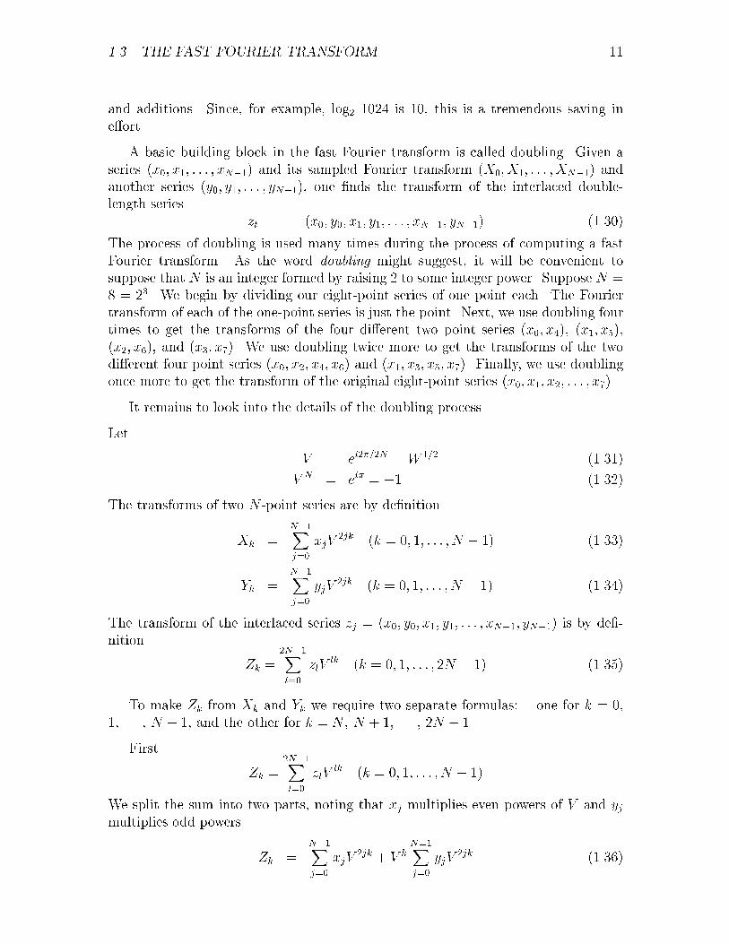
A basic building block in the fast Fourier transform is called doubling� Given aseries x�� x�� � � � � xN��� and its sampled Fourier transform X�� X�� � � � � XN��� andanother series y�� y�� � � � � yN���� one �nds the transform of the interlaced double�length series

zt x�� y�� x�� y�� � � � � xN��� yN��� �����

The process of doubling is used many times during the process of computing a fastFourier transform� As the word doubling might suggest� it will be convenient tosuppose that N is an integer formed by raising � to some integer power� Suppose N � ��� We begin by dividing our eight�point series of one point each� The Fouriertransform of each of the one�point series is just the point� Next� we use doubling fourtimes to get the transforms of the four di�erent two point series x�� x��� x�� x���x�� x�� and x�� x��� We use doubling twice more to get the transforms of the twodi�erent four point series x�� x�� x�� x� and x�� x�� x�� x��� Finally� we use doublingonce more to get the transform of the original eight�point series x�� x�� x�� � � � � x���

It remains to look into the details of the doubling process�

Let

V ei����N W ��� �����

V N ei� �� �����

The transforms of two N �point series are by de�nition

Xk N��Xj��

xjV�jk k �� �� � � � � N � �� �����

Yk N��Xj��

yjV�jk k �� �� � � � � N � �� �����

The transform of the interlaced series zj x�� y�� x�� y�� � � � � xN��� yN��� is by de��nition

Zk �N��Xl��

zlVlk k �� �� � � � � �N � �� �����

To make Zk from Xk and Yk we require two separate formulas� one for k ���� � � � � N � �� and the other for k N � N � �� � � � � �N � ��

First

Zk �N��Xl��

zlVlk k �� �� � � � � N � ��

We split the sum into two parts� noting that xj multiplies even powers of V and yjmultiplies odd powers�

Zk N��Xj��

xjV�jk � V k

N��Xj��

yjV�jk �����

�� CHAPTER �� TRANSFORMS

Xk � V kYk �����

We obtain the last half of the Zk by

Zk �N��Xl��

zlVlk k N�N � �� � � � � �N � �� �����

�N��Xl��

zlVl�m�N k �N m �� �� � � � � N � �� �����

�N��Xl��

zlVlmV N�

l�����

�N��Xl��

zlVlm���l

��� Phase delay and group delay

This material was revised and included in my third book� ESA�PVI�

��� Correlation and spectra

This material was revised and included in my third book� ESA�PVI�

��� Hilbert transform

This material was revised and included in my third book� ESA�PVI�

���� HILBERT TRANSFORM ��

Figure ���� A program to do fast Fourier transform� Modi�ed from Brenner� Callingthis program twice returns the original data� SIGNI should be ��� on one call and��� on the other� LX must be a power of �� c����� �NR