1

Paper SAS6685-2016

Credit Risk Modeling in a New Era

Jimmy Skoglund, Wei Chen, Martim Rocha, SAS Institute Inc.

ABSTRACT

The recent advances in regulatory stress testing, including stress testing regulated by Comprehensive Capital Analysis and Review (CCAR) in the US, the Prudential Regulation Authority (PRA) in the UK, and the European Banking Authority in the EU, as well as the new international accounting requirement known as IFRS 9 (International Financial Reporting Standard), all pose new challenges to credit risk modeling. There is an increasingly sophisticated requirement on credit models to cover long-term survival projections as well as integration of economic forward-looking components. Models are also required at a more granular level. The fact that credit models are supposed to cover all the material risks in the underlying assets in various economic scenarios makes the models harder to implement. Banks are currently spending significant resources on the model implementation but are still facing issues due to long time from model development to model deployment and to a disconnection between the model development and implementation teams. Efficient model execution becomes valuable for banks to get timely response to the analysis requests. At the same time, models are subject to more stringent internal and external scrutiny. This paper introduces a suite of credit modeling approaches suitable for the new challenges and discusses how to implement these models in the risk modeling solutions from credit risk modeling leader SAS®. The solution helps banks overcome these new challenges and be competent to meet the regulatory requirements.

INTRODUCTION: THE CREDIT MODEL CHALLENGES

Credit risk is arguably the most significant risk to every classical banking institution. The traditional regulatory credit risk approach to risk capital (risk-weighted assets) take a Through The Cycle (TTC) approach or even a downturn adjusted approach for the risk parameters Probability of Default (PD), Loss Given default (LGD), and Exposure at Default (EAD). This can be seen as an attempt to stabilize banks’ regulatory capital requirements over the years. The regulatory stress testing exercises, starting in the wake of the 2007 financial crisis, introduced a new credit risk modeling paradigm where Point in Time (PIT) or best estimate forward looking macroeconomic credit risk projection approaches were introduced.. Macroeconomic stress testing is being officially adopted as a risk management standard by many jurisdictions in the world. As a result, multi-horizon credit modeling, based on macroeconomic scenarios, becomes increasingly important. The new international accounting standard for the recognition of the credit loss known as IFRS 9 (IASB 2014) has taken the same approach. The US financial standard (FASB 2015) is following suit as well.

In general the new credit risk modeling requirements can be summarized into three features. The credit risk chapter of Skoglund and Chen (2015) provides a more detailed review of the past and new credit modeling methodologies.

1. Forward looking macroeconomic scenario based

In the past individual credit assessment was mostly static, based on history, and invariant to the macroeconomic environment. For some banks, the macroeconomic environment was introduced in a second step when the credit models were applied in the credit portfolio economic capital modeling in Pillar 2 of the Basel Accord. Because of the limited focus of traditional credit score models on the macroeconomic environment, the upward trending housing market and low default rate prior to the financial crisis led the credit modeling to bias toward the optimistic side. The key of the new credit modeling requirements is to first call for a macroeconomic sensitive credit analysis based on a forward looking view that reflects scenarios that might not have existed in the available historical economic data. The macroeconomic driven credit modeling can also naturally capture the underlying factors for the systemic credit contagion that was overlooked in the past. The challenge of this requirement to the financial institutions is to consider models focusing on survival through a series of projected economic horizons rather than a credit score or rating at a certain point in time.

2. Multi-horizon path dependent

2

The other important requirement to the credit risk modeling for the stress testing and new accounting standard is the path dependency for a multi-horizon analysis. Most of the banking book credits are held to maturity and there is rarely a jump-to-default. True defaults happen as a consequence of migrations to increasing delinquency period by period. In the same time-frame, delinquent accounts can recover and be considered healthy once more. Careful credit risk analysis must recognize the credit deterioration long before the actual default. Such recognition has also been practiced through, for example, credit rating changes for the commercial exposures and tracking delinquency status for retail loans. Such past behavior not only affects the forecasting of the default but also models the cash flows in the future. For example, a forecasted delinquency might cause the shortage of cash inflow, which affects the net income and liquidity of a future period. On the other hand, the cure of a delinquency might bring in more cash flows and accrued interest plus fees to the bank. In addition, in a multi-horizon analysis a prepayment or modification of the loan can also change the cash flow patterns in the subsequent horizons which again can significantly impact the loss forecasting and cash flows.

All the major regulatory stress testing initiatives define multi-horizon regulatory macroeconomic scenarios where the full balance sheet stress testing must be projected with these scenarios. For example, US CCAR and DFAST are based on nine quarter scenarios and in Europe, EBA stress testing is based on twelve quarter (3 year) scenarios. The credit models themselves can of course have a different frequency such as monthly even if, say, quarterly projections are used. This is natural for retail portfolios, for example, where delinquency status is typically measured monthly due to the payment frequency.

For the best estimate of expected credit loss calculation in the new accounting standards such as IFRS 9, when an exposure’s credit quality significantly deteriorates or is impaired, the exposure is subject to a lifetime credit loss calculation based on a business-as-usual economic scenario. In other cases a 12 month best estimate of expected credit loss is used. In practice a bank might also use multiple economic scenarios as the basis for a best estimate of expected credit loss with probability weighting.

3. Increased granularity

The new stress testing and accounting standards also call for as much granularity as possible. In most cases the best practice is to project credit loss at the asset or loan level. For example, the Board of Governors of the Federal Reserve System (2013) has required the credit modeling for the US CCAR to be carried out at sufficient granularity to capture the exposure that reacts differently to risk drivers under stress scenarios. IFRS 9 expect credit loss (ECL) is similarly assessed at sufficiently granular level.

The increased granularity of the credit modeling significantly increases the computational requirements and at the same time demands better programming practices to optimize the modeling performance.

In this paper we first review the typical credit risk models that capture these new requirements and then introduce the SAS solution that helps ease the implementation and improve the execution performance of these new models.

BACKGROUND: THE TRADITIONAL USE OF MACROECONOMIC CREDIT MODELS

Traditional credit score models for retail portfolios focus on the score at a point in time using for example, origination information and current status of the borrower. A score or probability of default is derived from the model. In most cases the outcome modeled is a default or no default event.

Traditional credit models for the commercial portfolios focus on the rating migrations in the rating scales assessed by external rating agencies such as Standard and Poor’s or Moody’s. The rating assessment and the empirical transition probabilities in the transition matrix are frequently based on long-term history covering many business cycles.

As we have mentioned before, with the Basel Pillar 2 adoption many banks implemented their own firmwide credit portfolio economic capital models. The implementation was often based on the standard

3

macroeconomic industry models such as CreditMetrics (1997), CreditPortfolioView (Wilson (1997)) and CreditRisk+ (1997). See Skoglund and Chen (2015) for an overview. The objective was to contrast the Pillar 1 capital requirements with the internal economic capital model. Hence, both the retail and commercial credit models were extended to include macroeconomic variables. At this time there was naturally much research activity on how to further enhance the standard industry models, for example, Nyström and Skoglund (2006) generalized the CreditPortfolioView approach to credit economic capital by introducing a full dynamic transition matrix approach. The model was based on a two-step calibration procedure. In the first step the traditional score or probability of default of the loan is obtained over a period of time and mapped to internal risk grades. Secondly, using the empirical transitions between risk grades a multinomial logistic transition model is fitted that depends on the macroeconomic factors. This yields a dynamic transition matrix for the portfolio with transition rates that are sensitive to the economic scenario. Similar approaches to dynamic transition matrix analysis were also developed and were usually based on the ordered probit model. For example, Nickell et al (2000) consider estimation of transition matrices that depend on macroeconomic variables. They consider an ordered probit model that allows a transition matrix to be conditioned on the business cycle and other factors such as industry. Belkin et al (1998) use a default/no default mode macroeconomic credit transition model based on the ordered probit that is generalized by Wei (2003) to multiple credit states. Wei (2003) models the deviation of the conditional transition matrix from the long-term, unconditional, transition matrix. The deviation model is referred to as a Z-score model that is a standard normal regression depending on the common macroeconomic factor and rating grade specific factors. The term Z-score relates back to the famous Altman (1968) Z-score model for bankruptcy prediction. More recently, Forster and Sudjianto (2013) consider a so-called EMV decomposition of the dynamic transition matrix with exogenous (macroeconomic) variability (E), maturity (time since origination; M) and vintage (V). Bellotti and Crook (2014) use discrete survival analysis with macroeconomic co-variates to stress retail portfolios. They generate a distribution of outcomes from a set of macroeconomic scenarios and use a risk measure approach to select a particular (set of) stressed outcomes. Berteloot et al (2013) apply macroeconomic (business cycle) credit migration modeling to a corporate portfolio using logistic regressions.

While both the macroeconomic retail and commercial models traditionally used for the banks can in principle accommodate multi-horizon analysis with path-dependency, many banks use the models only for a single, 1-year horizon economic capital projection. Subsequently the total 1-year horizon economic capital risk is contrasted with the 1-year horizon regulatory risk capital requirement from Pillar 1. Of significant interest is the difference due to concentration risk captured in the economic capital model as well as the implications to relative risk (capital) consumption by assets or loans.

MODELING: MACROECONOMIC CREDIT MODELS FOR STRESS TESTING AND IMPAIRMENTS

With the introduction of macroeconomic based stress testing and ECL analysis requirements the traditional credit portfolio economic capital models are not made obsolete. In fact, they become more important. However, there is a focus on deploying these models in path-dependent projections as well as capturing more exactly the dynamics along the path. Such path dynamics can include different delinquency behavior as well as so-called rating momentum. On the retail side it is obvious that delinquency status and delinquency path are important predictors of future credit quality. On the commercial side empirical evidence has been reported in the literature with respect to the impact of previous corporate downgrades or upgrades on future transitions (that is, rating momentum). For example, Cantor and Hamilton (2004) find that past rating history is important for predicting corporate default - violating the Markov feature for Moody’s transition matrices. Guttler and Raupach (2008) apply a credit transition model that is sensitive to past rating downgrades and compare with a credit transition model that is insensitive to past downgrades. They analyze the Value at Risk differences between the models and find potential significant underestimation with the rating momentum insensitive Value at Risk model.

In this section we consider general state transition models and how one can use state transition sampling or (expanded) Markov iteration to compute the associated expected loss given a single stress scenario for a set of economic risk factors. We also consider some specific models frequently used in the industry to compute stressed transitions for credit books and the associated loss. The specific models include

4

those used for large corporate and wholesale exposures as well as retail exposures. Our focus in this section is more on the structure of the models rather than their actual calibration to data. Of particular interest is how the models can be "solved" and hence used in stress testing execution to compute for example, default and expected loss flows conditional on a macroeconomic scenario. We focus on state transition model representations with multiple states. Simpler models such as default mode only models are special cases of this formulation. Default mode only models examples include parametric duration models such as the Weibull model as well as nonparametric duration models such as the Cox (1972) proportional hazard model. In default mode only models the default term-structure is usually an input to the model. For example, in the Weibull duration model the shape parameter controls the term-structure to yield increasing, flat, or decreasing term-structures appropriate for good, medium, and bad grade credits, respectively. In the nonparametric proportional hazard model the term-structure is usually embedded in the baseline hazard. In state transition models with multiple competing states (credit qualities) the resulting upward sloping, flat (or hump-shaped), decreasing term structure according to credit quality is usually a consequence of the state transition matrix and the subsequent migration paths that can happen. This is clearly an advantage of the model. We refer to Lancaster (1990) for an excellent introduction to the classical duration models.

Our exposition in this section will draw significantly from Skoglund and Chen (2016) as well as Skoglund and Chen (2015). However, we will avoid technical and mathematical details in this paper and we refer the reader to those references for the details

CREDIT MIGRATION AND STATE TRANSITION MODELS

State Transition Matrix Representation

We consider the discrete time state transition probability matrix, A[i,t], for i=1,...,n and times t=1,...,T. Here i=1,..,n represents the actual credit objects for which we are modeling the credit state transitions. In the retail banking book i=1,...,n usually denote loans while for the wholesale exposures and the trading book i=1,..,n can refer to issuer counterparties or specific bond exposures. We will refer to t=1,..,T as the future times for which we can obtain a predicted state transition matrix, A[i,t], conditional on the realization of the economic scenario, Z(t), and other relevant variables determining the transition probabilities. Such variables can include static idiosyncratic variables such as region of the borrower; age-indexed variables, such as loan age and economics; as well as dynamic variables that depend on past transition history such as realized delinquency spells and their severity. The times before t=0, denoting today, could have been used to calibrate the transition probability models although at this point we don't have to be explicit about the model calibration approach.

We assume that there are k=1,....,K possible states in the state transition probability matrix where d(r,l,t) is the probability that state r is entered at time t after state l at time t-1 given the history of the process up to time t. That is, the past state transition history. We assume that at t=0, each i=1,...,n, is located in one of the states 1,2,…,K-1. We therefore have, for each i, a K×K matrix of transition probabilities. The last row of A[i,t] defined as [0 0 ⋯ 0 1] as the default state K is an absorbing default state. While we have explicitly denoted the default state in the transition matrix as the last absorbing state, there can of course be multiple absorbing states. For example, in practice we might also need to handle the fact that some credit exposures exit the portfolio at times without defaulting on their obligations, due to prepayments, for example. By definition we have that transition probabilities for a row in the transition matrix must sum to unity. Migration can happen between any two states for which the transition probability is nonzero. Such states are usually referred to as competing states.

Simulation of State Transitions

To simulate a new state r for i=1,...,n in our discrete time state transition model we take as given a state transition matrix, A[i,t]. Here, the transition matrix is a matrix-valued stochastic process. However, conditional on a realization for the transition model(s) explanatory variables it is deterministic. The exact realization of Z(t) is of course determined by the exact economic scenario specification.

Now, assuming that each row of the transition matrix is normalized to sum to unity, using normalization or an explicit multinomial model specification, we sample a uniform random variable u. Given the sampled u we have that the transition state of i=1,...,n, previously in state l, is determined by the K-dimensional

5

transition indicator d[i,t] where element k is unity if and only if the transition occurs to state k. The sampling at t=1,…,T creates a state transition path, j. Assuming that we are searching for the expected credit loss we can then average the estimated expected credit loss across the j=1,…,M paths. The implementation of this type of state transition simulation algorithm is trivial in practice. The drawbacks of the state transition simulation approach are that it is not exact and that in general a large number of state transition paths are needed for accuracy. Especially since default is a remote event and might for example, only happen as a consequence of period by period migrations to worse delinquency events.

Markov Iteration of State Transitions

In any state transition model we can of course sample j=1,...,M state transition paths conditional on the economic scenario and then obtain for example, expected scenario loss. However, we can also try to compute the expected state occupancy probabilities using Markov iteration. For example, it is well-known (see for example, Lancaster (1990)) that for a time-inhomogeneous Markov chain that does not depend on past state transition history we have a simple expected state occupancy, x, iteration relation using the updated state transition matrix and the past state occupancy:

x[i,t]=A’[i,t]x[i,t-1].

In this Markov model we can also easily incorporate portfolio growth and decay rates (amortization). When the transition models depend on past transition behavior, such as past delinquency history or rating momentum, the corresponding Markov iteration can become very complex. This is because we need to track the past state occupancy. However, in practice many “non-Markov” models only track a few discrete events such as month since last delinquent, ever delinquent 90 days before, and so on. Skoglund and Chen (2016) therefore consider an expanded conditional Markov iteration that conditions on these events and is still tractable. This is an important insight because when using simulation of state transition paths to solve a non-Markov model we require in general many paths in the order of 100,000 – 1,000,000 to have accurate results at the loan level. As we have mentioned this is because many credit events are remote and moreover might only happen as consequence of period migrations. This makes the requirement on the number of state transition simulations even greater. Therefore, a Markov iteration approach is preferred in practice if available. Especially in cases where accurate loan-level expected credit losses are required such as in the ECL calculation for IFRS9.

Specific State Transition Models

Commercial Models

The multivariate version of the Merton (1974) model of defaultable corporate bond pricing is often used to model corporate default and rating migration. Standard industry models such as the CreditMetrics (1997) model stem from this approach and use factor models where the underlying factors are macroeconomic variables. In the CreditMetrics approach different states cut-off levels are calibrated based on empirical default and transition data. In the frequently used multi-factor approach a set of macroeconomic factors are linked to the credit health of the corporate through a linear regression model. Conditional on the resolved credit health index the credit quality state is obtained from comparison with a long-run state transition matrix such as the published state transition matrices by the rating agencies. The calibration of the model includes both a selection of economic indices to use as well as their weights. Such a calibration can either use expert judgment or regression techniques. In the latter case the unobserved corporate credit health index is often approximated by equity. Subsequently the transition matrix transition probabilities are transformed to conditional (on the macroeconomic factors) transition probabilities. The resulting dynamic transition matrix can be mathematically expressed as a multinomial probit model conditional on the economic factors. Taking an expectation on the conditional state distribution (that is, using a law of large numbers) the model can be seen as a time-inhomogeneous Markov chain and hence has analytic expected credit loss. This is an important feature of the model as the “solving” of the model for stress testing or lifetime credit loss reduces to updating a simple Markov iteration equation at each t=1,…,T.

We have previously discussed that commercial models might also have “non-Markov” features such as rating momentum. The rating momentum is usually modeled in this model context as switching state transition matrices conditional on rating events. This is because such different transition matrices can

6

usually be estimated on data (see Guttler and Raupach (2008)). Because the non-Markov events are usually limited, for example, recent downgrade indicator, it means that the model can still be solved with an expanded conditional Markov iteration instead of simulation of state transition paths.

Retail Models

Just like the commercial models the retail models can also be based on state transition matrices. The states might be for example, internal credit grades or different delinquency status such as current, past due 30 days, and past due 60 days. Since for the retail segment there is generally more data available for calibration (panel or cohort data) a variety of regression-based approaches are used such as logistic regression, proportional hazard models, and so on. The different models for each cell of the state transition matrix can be estimated together and retain the conditions of the transition matrix such as when using multinomial logistic models for a row of the transition matrix. The models can also be estimated as atomic models that is, separate models for each transition from and to state. See Bellotti and Crook (2013) for an example of discrete survival model calibration (with a logistic model) to a conditional default or delinquency indicator using both static application variables, macroeconomic variables, and behavioral delinquency variables.

When the model only considers segmentation (static) and macroeconomic variables for determining the state transition probability, the model is a time-inhomogeneous Markov chain that does not depend on past state transition history. It can therefore be solved with a simple Markov iteration. On the other hand, if the model includes past state transition history – usually in the form of past delinquency events such as months since last delinquent or ever delinquent 90 days before – one either has to resort to a more complex expanded Markov iteration or state transition simulation. As detailed in Skoglund and Chen (2016) a delinquency state transition model typically has only l=1,…,L discrete events that need to be tracked and can therefore often be solved with a slightly expanded conditional Markov iteration rather than requiring simulation. However, in practice one must carefully analyze the model and see if a Markov iteration scheme is too complex to implement and instead if it is preferable to resort to sampling.

IMPLEMENTATION: SAS® MODEL IMPLEMENTATION PLATFORM

The implementation of credit models for the purpose of stress testing and impairment calculation faces many challenges in practice. Such challenges include:

Having a structured and timely process for moving models from development to implementation.

Having an optimal implementation that require strong knowledge in both modeling and computer science.

Having a modeling framework that supports factors like multiple model families, competing risks, models with both static, economic, and dynamic variables (for example, delinquency tracking), collateral models, loan dynamics, and cash flow projections, ability to define custom measures for example, EBA impairments or IFRS9 lifetime expected credit loss.

Having the ability to do what-if analysis such as application of new macroeconomic scenarios and sensitivity analysis as well as easy comparison of champion and challenger models.

A timely model execution time even on very large portfolios.

The SAS® Model Implementation Platform was designed to address these challenges for banks. It supports model import from model metadata, generates optimal parallel code based on the model metadata, and allows the user to bring together all the different models (for example, state transition models, severity models, collateral haircut models, and facility drawdown models) that need to work in concert for a particular application against a portfolio or sub portfolio

1.

1 The fact that model metadata is used to import models means that models do not have to be estimated

in SAS.

7

The SAS® Model Implementation Platform provides user with a flexible way to define their own calculation logic for example, stress test or ECL calculation logic using the models. Once a set of models are chosen to run against a portfolio, the user can choose one or multiple economic scenarios to use for the projection. The results are held in memory for users to explore dynamically down to the most granular level and to compare the results under different economic scenarios and model choices.

AN OVERVIEW OF THE SAS® MODEL IMPLEMENTATION PLATFORM WORKFLOW

Model Execution Library

The model execution library stores all models of the different model types needed for the analysis such as default probability models, loss given default models and exposure models. Users can view all the models or a filtered list of models in the library.

Display 1. Model Execution Library

The Model Implementation Platform does not require full model code but the key model information such as model attributes, model variables, and parameters. This allows the system to generate consistent code for a model when it is going to be used. It does not matter on which estimation platform the model is developed. From the model execution library a user can choose a particular model to see its details. The example below is from a logistic model that has been calibrated on the basis of the odds-ratio and hence returns an odds-ratio. The sample model is also part of a transition matrix and consequently has from and to state assigned to it.

8

Display 2. Model Library Model Details

Model Groups and User-defined Logic

Once the user has imported the models that are to be used, the next step is to group models together for the purpose of applying them to the portfolios for one or multiple analyses such as loss and cash flow projection. The figure below shows examples of a few model groups already created.

Display 3. Model Groups

Within a particular model group the user selects which models (model associations) to use and assigns output variables. Within a particular model group the user also defines the calculation logic that applies to the models. It includes any pre- or post-model logic, connections between models and output variable derivation from the models. If applicable to the model group, a user can also generate one or many transition matrices. The system makes it easy for the user to set up a transition matrix through its defined states and associate transition probability models through the from and to states already defined in the models. Since the system is already set up to handle path-dependent multi-horizon logic, a model group only needs to define the logic for computation within one horizon and how a cross horizon variable should get its value in one particular horizon. Display 4 illustrates the model group components.

9

Display 4. Model Group Details

Model Group and Portfolio Mapping

Once the model groups have been created by the user, the next step is to map the model groups to sub portfolios. This is the step where the user tells the system how to treat a specific sub portfolio. The mapping mechanism allows the user to easily apply different model groups to a sub portfolio in case different calculation are to be explored. Display 5 shows that the retail and corporate parts of the portfolio use different model groups

Display 5. Model Mapping to Portfolios

Model Execution

When the model group to portfolio mapping has been assigned, the next step is typically to run the analysis. The user can choose different combinations of portfolio, scenario, and model group mappings and, for example, champion or challenger model groups to try different what-if scenarios in different runs. The system will generate optimal code and automatically distributes the portfolio for massively parallel and in-memory processing. Each execution instance is kept in the system with its generated code, logs, output data sets, and result exploration link. Display 6 is a view of model execution and run instance list.

10

Display 6. Model Execution

Results Exploration and Analysis

Once the results have been generated, the user can explore the results using the risk explorer. The risk explorer uses the in-memory technology to allow the user to drill down into ad hoc portfolio hierarchies, select output measures, and scenarios to view. Results can be displayed graphically such as in the example shown in Display 7 where expected loss is displayed for three different economic scenarios for the retail portfolio with internal rating grade INT1.

Display 7. Results Exploration and Analysis

11

Ad Hoc Scenario Definition and Application

In addition to using the economic scenarios provided with the model execution users can also create ad hoc multi-horizon scenarios on the fly and run them against the portfolio. The risk scenario manager has all the model variables that a user wants to create scenarios for as well as additional risk factors such as foreign exchange rates and interest rate curves. The factors are displayed as risk sources and the grouping of the factors is user defined. The user can build multi-horizon scenarios by perturbing selected variables at individual, curve, and group levels. Graphical exploration and perturbation of the scenario for the variable are also possible. Display 8 is an illustration of one scenario.

Display 8. Scenario Management and Definition

TWO EXAMPLE IMPLEMENTATIONS IN THE SAS® MODEL IMPLEMENTATION PLATFORM

In this section we illustrate the concrete implementation of a couple of models in the SAS® Model Implementation Platform. Our first model example uses time-inhomogeneous Markov state transition matrices for retail and commercial portfolios to compute IFRS9 ECL and EBA stress testing required outputs. Our second model approach uses dynamic state transition matrices with delinquency tracking to compute stressed default rates and losses. The scope of the SAS® Model Implementation Platform is broader than the model types we consider here and also covers, for example,duration models with competing risks and simple vintage curve or roll rate models implementation.

A MARKOV STATE TRANSITION MODELS EXAMPLE

The Markov state transition models process is outlined in Figure 1. The corporate portfolio part uses macroeconomic multi-factor models for each corporate and a state transition matrix. It also uses collateral models segmented on type and region of the collateral together with haircut models to calculate collateralized recovery value. The retail part of the portfolio uses a dynamic transition matrix approach that is calibrated on the log-odds ratios of the historical transition rates to the macroeconomic factors. As for the corporate models there are collateral models segmented on collateral type and region as well as collateral haircut models.

12

Figure 1. The Markov State Transition Models

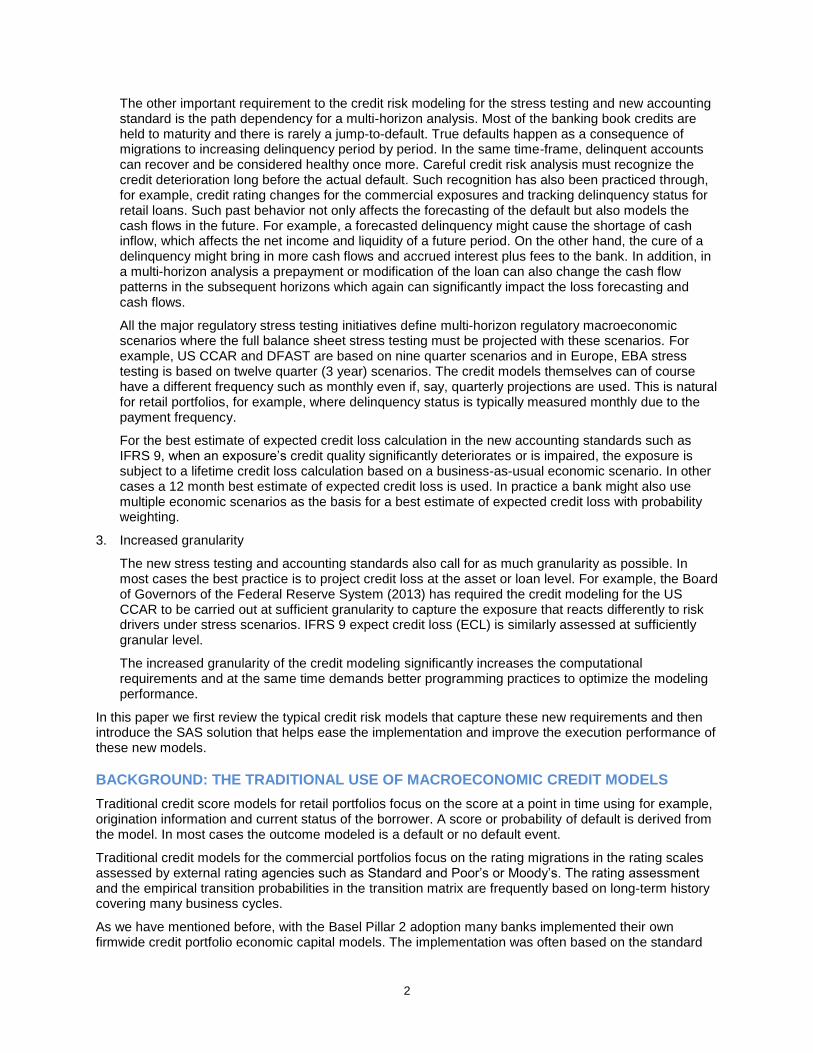
Display 9 shows the retail portfolio transition matrix. All the transition rates in the matrix are dependent on a GDP index. The corporate transition matrix looks similar in structure. The corporate transition matrix is constant while each corporate has a multi-factor model (macroeconomic factor model) to convert the constant transition probabilities to point in time (PIT) transition probabilities. A sample multi-factor model is shown in display 10.

Display 9. Retail Transition Matrix

13

Display 10. Sample Corporate Multi-factor Model

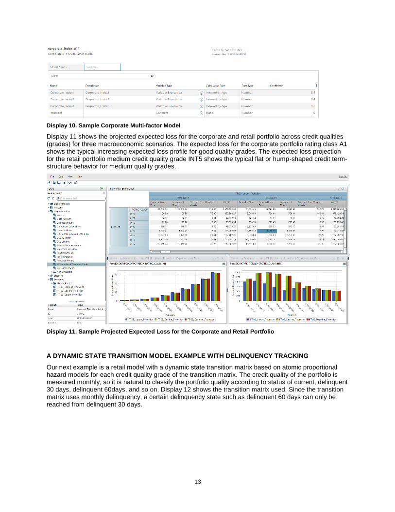
Display 11 shows the projected expected loss for the corporate and retail portfolio across credit qualities (grades) for three macroeconomic scenarios. The expected loss for the corporate portfolio rating class A1 shows the typical increasing expected loss profile for good quality grades. The expected loss projection for the retail portfolio medium credit quality grade INT5 shows the typical flat or hump-shaped credit term-structure behavior for medium quality grades.

Display 11. Sample Projected Expected Loss for the Corporate and Retail Portfolio

A DYNAMIC STATE TRANSITION MODEL EXAMPLE WITH DELINQUENCY TRACKING

Our next example is a retail model with a dynamic state transition matrix based on atomic proportional hazard models for each credit quality grade of the transition matrix. The credit quality of the portfolio is measured monthly, so it is natural to classify the portfolio quality according to status of current, delinquent 30 days, delinquent 60days, and so on. Display 12 shows the transition matrix used. Since the transition matrix uses monthly delinquency, a certain delinquency state such as delinquent 60 days can only be reached from delinquent 30 days.

14

Display 12. Monthly Delinquency Transition Matrix

Display 13 shows a sample atomic proportional hazard model in the transition matrix. All the transition models depend on a macroeconomic factor (unemployment index) as well as delinquency status variables including months since last delinquent, ever delinquent 60days, and so on. Because the model depends on variables that track delinquency status, the model is non-Markov. This means that the expected loss (conditional on a macroeconomic scenario for the unemployment index) has to be solved by either simulation of state transition paths or an expanded conditional Markov iteration.

Display 13. Sample Atomic Proportional Hazard Model in the Transition Matrix

Display 14 shows the portfolio projected loss amount using a million state transition paths when the loan is in state current at the start. It also shows as overlay the corresponding projected expected loss profile using an exact expanded conditional Markov iteration. Even with such a large number of state transition paths as a million there is still some randomness compared to the smooth Markov path. This is because the sample portfolio is small such that randomness is not averaged away. Clearly, loan level accurate results require many state transition paths while accurate results on a large portfolio can benefit from the law of large numbers when aggregating loan results.

15

Display 14. Portfolio Projected Loss Amount with State Transition Simulation and the Exact Expanded Conditional Markov Iteration (in the highlighted chart)

CONCLUSIONS

The financial crisis in the last decade calls for the evolution of the credit risk modeling to more accurately capture the behavior of the loans sensitive to macroeconomic dynamics at granular level. Banks are facing methodological and technical challenges from the new era of credit risk modeling. SAS® Model Implementation Platform provides a platform for banks to implement and execute their credit models in a structured way with a timely process for moving models from development to implementation. The modeling framework supports multiple model families including competing risks, models with static, economic, and dynamic variables (for example, delinquency tracking), collateral models, loan dynamics, and cash flow projections. Users can also define custom measures and model calculation approaches easily. In addition to supporting the model execution the SAS® Model Implementation Platform makes it easy to carry out what-if and sensitivity analysis of models together with a timely model execution time even on very large portfolios.

The SAS® Model Implementation Platform can manage both simple and complex models as well as multiple types of analytical model executions in concert. This includes the traditional retail and commercial macroeconomic credit models that can often be efficiently implemented using conditional Markov iteration as well as the more complex dynamic models that require state transition simulation or an expanded conditional Markov iteration to produce forecast of losses, impairments, future balances, and so on.

REFERENCES

Altman, E. I (1968), Financial Ratios, Discriminant Analysis and the Prediction of Corporate Bankruptcy, Journal of Finance, September, pp. 189-209.

Belkin, B, Suchower, S, and Forest Jr. L (1998), A One-Parameter Representation of Credit Risk and Transition Matrices, CreditMetrics Monitor, Third Quarter.

Bellotti, T and Crook, J (2104), Retail Credit Stress Testing using a Discrete Hazard Model with Macroeconomic Factors. Journal of the Operational Research Society, 65, pp. 340--350.

16

Bertelot, K, Verbeke, W, Castermans, G, Van Gestel, T, Martens, D and Baesens, B (2013), A Novel Credit Rating Migration Modeling Approach Using Macroeconomic Indicators, Journal of Forecasting, 32 (7), pp. 654--672.

Cantor, R and Hamilton, D (2004) , Rating Transitions and Defaults Conditional on Watchlist, Outlook and Rating History, Moody’s special comments.

Cox, D. R (1972), Regression Models and Life Tables, (with discussion), Journal of the Royal Statistical Society, 34, pp. 187-220.

CreditRisk+ manual, (1997), available from http://www.csfb.com/creditrisk.

CreditMetrics manual, (1997), JP Morgan.

Forster, J and Sudjianto, A (2013), Modelling Time and Vintage Variability in Retail Credit Portfolios: The Decomposition Approach, working paper, Lloyds Banking Group.

Guttler, A and Raupach, P (2008), The Impact of Downward Rating Momentum on Credit Portfolio Risk, Deutsche Bundesbank, Discussion Paper Series 2: Banking and Financial Studies, No 16.

Lancaster, T (1990), The Econometric Analysis of Transition Data, Cambridge University Press.

Merton, R. C (1974), On the Pricing of Corporate Debt: The Risk Structure of Interest Rates, Journal of Finance, Vol 29 (2), pp. 449-470.

Nickell, P, Perraudin, W and Varotto, S (2000), Stability of Rating Transitions, Journal of Banking and Finance, 24, pp. 203-227.

Nyström, K and Skoglund, J (2006), A Credit Risk Model for Large Dimensional Portfolios with Application to Economic Capital, Journal of Banking & Finance, 30, pp. 2163-2197.

Skoglund, J. and Chen, W. (2015). Financial Risk Management – Applications in Market Risk, Credit Risk, Asset and Liability Management and Firmwide Risk. Wiley Finance.

Skoglund, J and Chen, W (2016), The Application of Credit Risk Models to Macroeconomic Scenario Analysis and Stress Testing, forthcoming Journal of Credit Risk.

Wei, J. Z (2003), A Multi-Factor, Credit Migration Model for Sovereign and Corporate Debts, Journal of International Money and Finance, 22, pp. 709-735.

Wilson, A (1997), Portfolio Credit Risk. Risk Magazine 9, pp. 111-117, and 10, pp. 56-61.

CONTACT INFORMATION

Your comments and questions are valued and encouraged. Contact the author at:

Jimmy Skoglund SAS Institute Inc. jimmy.skoglund@sas.com Wei Chen SAS Institute Inc. wei.chen@sas.com Martim Rocha SAS Institute Inc. martim.rocha@sas.com

SAS and all other SAS Institute Inc. product or service names are registered trademarks or trademarks of SAS Institute Inc. in the USA and other countries. ® indicates USA registration.

Other brand and product names are trademarks of their respective companies.