Paper : Football (Soccer) A DEA Approach to Evaluating ... · DEA allows a relative evaluation...

DEA Approach to Evaluation of J-league Players

Football Science Vol.13, 9-25, 2016http://www.jssf.net/home.html

9

1. Introduction

Data envelopment analysis (DEA) is a method of obtaining a relative evaluation of the efficiency of study subjects utilizing the ratio of outputs to inputs. This method is often used in analyzing the efficiency of business organizations (e.g. Copper et al., 2007). It is also used to evaluate the efficiency of teams and players in baseball and soccer. When applied to sports teams, DEA can evaluate efficiency in terms of number of wins against total annual salary of players, in other words, the efficiency of winning with lower total annual salaries (e.g. Lewin et al., 2013). Applied to players, DEA can evaluate efficiency according to position in terms of successful goals, assists, passes, and tackles against time played (Tiedemann et al., 2011), or can rank players in terms of games played and successful goals (Santin, 2014).

Hirotsu et al. (2012) focused on the characteristics rather than the rank of each soccer player. They used annual data from the J-League Division 1 (J1)

in 2008, used time played as an input, and used successful basic plays such as goals, passes, and dribbles as outputs for analysis applying the Charnes-Cooper-Rhodes (CCR) model (e.g. Copper et al., 2007), the most basic DEA model, to extract the characteristics of each player and indicate target values for improvement. Their study was significant for its attempt to extract the characteristics of according to player using DEA to evaluate the frequency of basic plays in combination with multiple items. In other words, when evaluating each player based on frequency of basic plays, not only did they separately evaluate the frequency of successful goals and crosses, but also the combined frequency of both successful goals and crosses to identify the characteristics of each player for evaluation based on a 0 to 1 index of “efficiency.” DEA was also applied to evaluate player similarity, which also includes frequency of basic plays between players.

In general, team “efficiency” is calculated as a function of cost; that is, the number of wins per year

A DEA Approach to Evaluating Characteristics of J-League Players in terms of Time played and Player Similarity

Nobuyoshi Hirotsu* , Kiyoshi Osawa**, Yukihiro Aoba*** and Masafumi Yoshimura*

*Graduate School of Health and Sports Science, Juntendo University**Japan Institute of Sports Sciences, Japan Sport Council

***School of Health and Sports Science, Juntendo University1-1 Hiragagakuendai, Inzaishi, Chiba 270-1695, Japan

[email protected][Received November 4, 2014; Accepted October 8, 2015]

In this paper, J-league player performance was evaluated using data envelopment analysis (DEA) models to identify player characteristics from the standpoints of time played and player similarity. For this purpose, the concepts of scale efficiency and super efficiency were introduced to this study. Time played was used as the input and data from ten basic plays or actions such as goals, passes, dribbles and fouls, were used as the outputs. The performance of J-league field players was analyzed according to player position using data from the 2013 season based on the CCR (Charnes-Cooper-Rhodes) and BCC (Banker-Charnes-Cooper) models. Characteristics were discussed in reference not only to efficiency scores, but also scale efficiency and super efficiency scores. The suitability of player time on pitch was identified by scale efficiency with estimation of returns to scale. Efficient players were differentiated by super efficiency scores, and the relationship between efficient players was quantified with regard to the characteristics of plays in the position.

Keywords: BCC, DEA, Evaluation, Scale Efficiency, Super Efficiency

Paper : Football (Soccer)

[Football Science Vol.13, 9-25, 2016]

Football Science Vol.13, 9-25, 2016

Hirotsu, N. et al.

http://www.jssf.net/home.html10

against total annual player salaries. Although the analysis conducted by Hirotsu et al. (2012) used the term “efficiency” as defined by DEA, they simply focused on the frequency of successful individual goals and passes during a game by defining success as a function of the higher number of goals or passes. In other words, considering basic plays in a comprehensive manner, a player whose efficiency score is “1” has a specific characteristic of frequency that cannot be seen in other players.

H i r o t s u e t a l . ( 2 0 1 2 ) e v a l u a t e d p l a y e r characteristics utilizing the CCR model. However, the CCR model is based on constant returns to scale. Evaluation requires that the ratio of frequency of plays to time played is constant regardless of the actual time played. If the time played doubles, the frequency of basic plays doubles. This CCR model is problematic due to the fact that it obtains efficiency scores based on time played without considering the difference of impact caused by the length of time played between players with longer and less time played. Hirotsu et al. (2012) also found a relationship between efficient and inefficient players utilizing the CCR model. However, analysis utilizing CCR model alone can neither quantify the difference in characteristics among players with an efficiency score of “1,” nor find similarity in characteristics among efficient players. Therefore, the CCR model has limitations as an analytical method for the evaluation of player characteristics.

To address these issues, we should employ both the Banker-Charnes-Cooper (BCC) model and the concept of super efficiency for analysis. BCC models variable returns to scale, which can evaluate player efficiency scores and scale efficiency considering player time on pitch. This makes it possible to analyze data that fully considers the characteristics of each player from the standpoint of whether the player should play more or less in the season, and determine suitable time played for each player. This is a completely different evaluation based on “scale efficiency”.

The concept of super efficiency allows us to observe the differences in characteristics of players with efficiency scores of “1,” which allows us to perceive similarity in characteristics among efficient players. The concept of super efficiency allows an efficiency score greater than 1, which Santin (2014) also adopted. The implementation of the concept of super efficiency makes it possible to

efficiently quantify the similarity of efficient players’ characteristics and to evaluate the characteristics of a player based on a combination of other players, which could be useful in player recruitment.

This study was carried out to analyze the performance of J1 players in terms of appropriate time played, difference and similarity in player characteristics based on the study by Hirotsu et al. (2012) adopting the BCC model and the concept of super efficiency, and to compare evaluation utilizing the CCR model with evaluation utilizing the BCC model and the concept of super efficiency.

2. Method

2.1. Data

For analysis in this study, we first selected data in accordance with the study by Hirotsu et al. (2012). We selected time played as an input, and frequency of ten major plays such as goals and passes as outputs as shown below.

Input (1 item): Time playedOutputs (10 items): Number of goals, assists,

passes, crosses, dribbles, tackles, intercepts, clearances, blocks, and fouls

(Note) Passes: Number of passes to a team playerCrosses: Number of crosses to a team playerDribbles: Number of successful dribblesFouls: Difference from the maximum number

of fouls after conversion with time played (Evaluated as a grade)

Although fouls were used as an output, it is of greater advantage to have a lower number different from other outputs. Therefore, we converted data for evaluation. Hirotsu et al. (2012) set the base number of fouls per unit time at 78 times/ 1414 minutes (0.05512 times/ min.) utilizing the data of S. HIRAYAMA who committed the maximum number of fouls in 2008. This study set the base number per unit time at 53 times/ 1287 minutes (0.04118 times/ min.) by WELLINGTON from 2013 data.

We acquired 2013 J1 data aggregated by Data Stadium Inc. and evaluated the above-mentioned 11 input and outputs for players who played more than 900 minutes according to their registered position.



11

Subjects were 238 players; namely, 57 forwards (FW), 95 mid fielders (MF), and 86 defenders (DF). A summary of evaluation item statistics according to their position is shown in Table 1.

FW goals, assists, passes, crosses, and dribbles in the shaded area of Table 1 are in order of frequency, as shown in Table 2. This shows FW characteristics. For example, Y. OKUBO ranked top in number of goals, and RENATO was top in number of assists and crosses, which reveal characteristics. Utilizing DEA, we can also identify player characteristics for multiple items. DEA obtains better analytical results than those acquired from frequency data.

2.2. Models

As for the DEA model, we will first explain the CCR model, followed by the BBC model and the concept of super efficiency.

2.2.1. CCR ModelDEA allows a relative evaluation employing the

ratio of inputs and outputs. If we define “goal rate” as the ratio of “goals/ time played,” the goal rate equals the ratio of “time played (input)” and “goals (output),” which evaluates player efficiency. Multiple items can be employed as inputs and outputs in DEA. If “passes” are added as outputs, the ratio is defined as “time played (input)” and “u1×goals+u2×passes” (output). The variables u1 and u2 express the weight

Table 1 Summary statistics

Table 2 Top and bottom players in terms of goals, assists, passes, crosses and dribbles for FW

PositionNo, ofplayers

Time Goals Asists Passes Crosses Dribbles TacklesInter-

ceptionsClears Blocks Fouls

(Foul Points)

57 Average 1906.4 7.7 2.9 435.7 7.2 21.8 19.0 3.1 20.2 22.5 35.6 (42.9)

SD 636.3 6.0 2.3 192.3 6.9 18.2 11.6 2.4 13.5 8.8 15.5 (23.9)

Max 2969 26 11 866 29 81 67 13 56 42 79 (91.6)

Min 937 0 0 162 0 1 4 0 0 5 15 (0.00)

95 Average 2142.3 2.3 3.0 916.8 9.5 15.1 39.6 9.1 34.4 42.8 28.2 (60.0)

SD 686.7 3.0 2.6 487.6 9.0 17.3 23.2 5.9 20.1 18.2 14.5 (22.4)

Max 3060 21 12 2910 44 105 130 24 128 83 65 (113.3)

Min 902 0 0 228 0 0 7 0 4 8 5 (15.8)

86 Average 2148.0 1.5 1.1 858.8 7.4 7.1 42.1 8.2 81.3 48.7 25.7 (62.8)

SD 674.4 1.6 1.5 413.2 11.5 10.7 19.3 6.0 33.4 18.0 11.6 (23.9)

Max 3060 9 8 2565 58 64 96 33 164 90 67 (109.9)

Min 910 0 0 187 0 0 10 0 10 17 5 (18.5)

FW

MF

DF

Remarks) * Recognized as outstanding players in 2013** Recognized as the best eleven in 2013

Player Goals Player Asists Player Passes Player Crosses Player Dribbles

Y.OKUBO** 26 RENATO* 11 RENATO* 866 RENATO* 29 RENATO* 81

K.KAWAMATA 23 J.TANAKA 11 K.TAMADA 857 Choi Jung-Han 26 JUNINHO 63

Y.TOYODA 20 KENNEDY 7 Y.OKUBO** 842 JUNINHO 23 CHO Young Cheol 61

Y.OSAKO** 19 M.SAITO* 6 LUCAS Severino 811 T.TAKAGI 22 Choi Jung-Han 61

M.KUDO 19 ・・・・・・ CHO Young Cheol 791 M.SAITO* 20 M.SAITO* 57

・・・・・・・・・・・・・・・・・・・・・・・・・・・・・・

・・・・・・・・・・・・・・・・・・ R.MAEDA 1 ・・・・・・

K.YANO 1 H.KANAZONO 0 A.YANAGISAWA 195 S.ITO 1 Y.MORISHIMA 5

Choi Jung-Han 1 WELLINGTON 0 QUIRINO 185 H.KANAZONO 0 HUGO 5

A.KAWAMOTO 1 A.KAWAMOTO 0 Radončić 174 HUGO 0 K.TAKETOMI 4

M.MATSUHASHI 0 HUGO 0 BARE 171 T.YAZIMA 0 H.KANAZONO 2

GILSINHO 0 K.TAKETOMI 0 T.YAZIMA 162 A.YANAGISAWA 0 A.YANAGISAWA 1


Hirotsu, N. et al.


of goals and passes. If an evaluator determines the weight u1 as 10 and u2 to be 1 considering the goal is ten times as important as the pass, the evaluation scale is influenced by evaluator bias. In order to avoid evaluator influence on DEA, we must select u1 and u2 values to obtain the maximum ratio; in other words, the highest evaluation. In such case, there is no deviation by evaluator, and all players can be evaluated by their most advantageous weight, which is fair for everyone. DEA sets a player with the maximum ratio as the standard (1) to evaluate each player with the efficiency score of 0 to 1. If a player cannot achieve an efficiency score of 1 even after evaluation with the most advantageous weight, the player is inferior to the players that had an efficiency score of 1. The model that evaluates subjects with such a ratio is CCR. Hirotsu et al. (2012) also evaluated players utilizing the CCR model.

2.2.2. BCC Model and Scale EfficiencyThe above-mentioned CCR model was developed

into the BCC model. We replace time played (input) with v1×time played+v0, and the v1 and v0 values were selected to obtain the maximum ratio for each player. The greater the increase in the number of variables, the greater the increase in the level of flexibility. This can convert to the multi-input-multi-output formula shown below. When the number of inputs is m and the number of outputs is s, data (xijo) regarding input i (=1,2,…,m) of a subject player (jo) was multiplied by weight (νi). Adding v0 to the result yields virtual

input i =1

vi xijo + v0

m∑ . The data (yrjo) regarding the output

r (=1,2,…,s) of a subject player (jo) was multiplied by

weight (ur). It yields virtual output ur yrjo

r =1

s∑

Virtual outputVirtual input

Ratio= =i =1

vi xijo + v0

m∑

ur yrjo

r =1

s∑

(1)

This is the ratio in the BCC model. The BCC model determines the suitable v0, νi, and ur of subject players to maximize (1) under non-negative conditions, and calculates efficiency scores. In the present study, we use one input and ten outputs; therefore, m=1 and s=10.

The significance of adding the new variable v0 can be explained in a case of one input and output utilizing “v1× time played + v0” as input and “u1×

number of goals” as output. Figure 1 shows the relationship between time played and goals of 57 FW in J1 during 2013. Point D in Figure 1 shows K. KAWAMATA (time played: 2503 min., number of goals: 23), and Point C shows G. OMAE (time played: 1207 min., number of goals: 7).

We compared CCR and BCC model ratios. The CCR model does not consider the variable v0 (i.e. v0=0). When there is one input and one output (m=1,s=10), formula (1) is described as shown below:

u1 y1jo

v1 x1joRatio = (2)

In this case, the player with the maximum goal percentage (goals/ time played) is K. KAWAMATA, who is shown as Point D, and the value equals the inclination of a straight line obtained by connecting the origin and Point D in Figure 1. If we set the ratio acquired by formula (2) at 1, the formula can be

described as u1 y1jo

v1 x1jo1 = which is equals

v1u1

x1joy1 jo = .

If we set the ratio of K. KAWAMATA as the standard value, as shown above, v1/u1 equals 23/2503, and 0.009189. This means that the straight line running through the origin with 0.009189 inclination becomes the CCR efficient frontier with the maximum goal percentage. At the point on this straight line, the ratio shown in formula (2) is 1, which means the efficiency value is 1.

Whereas, in the BCC model, we use the variable v0. When we set formula (1) as equal to 1 with one input and one output, the formula is described as

u1 y1jo

v1 x1jo + v01 = , which becomes

v1u1

x1jo +y1 jo =v0u1

.

In this case, the ratio of points on the straight line that does not pass through the original position (0,

Figure 1 CCR efficient frontier and BCC efficient frontiers

0

5

10

15

20

25

30

0 500 1000 1500 2000 2500 3000 3500

ED

T C

BA

CCR efficient frontier

BCC efficient frontiers

Time (min.)

Goa

l

P

P'



13

0) becomes 1. For example, in Figure 1, the ratio of points on the straight line that passes through Points C and D becomes 1. The inclination of the straight line is v1/u1=(23-7)/(2503-1207)=0.01235, and the interception is v0/u1=-7.901. If we consider the straight line that passes through Points A and B, the straight line that passes through Points B and C, and the straight line that passes through Points D and E similarly, the points that make formula (1) equal to 1 are on a polyline that passes through Point A, B, C, D, and E that covers all players shown in Figure 1; and that line forms the BCC efficient frontier. In the case of multi-input-multi-output, a boundary surface that covers all players forms the BCC efficient frontier although it cannot be shown in a figure here.

For example, Point T, which does not exist on the BCC efficient frontier line, describes J. TANAKA (time played: 2022 min., number of goals: 11). The 2022 min. point of time played on the CCR efficiency frontier line is on the straight line that passes through the origin (0, 0) with a 0.009189 inclination, and shows 18.58 (=0.009189×2022) as the number of goals. This should be the target value for improvement (Point P) for J. TANAKA in the CCR model. The point on the BCC efficiency frontier line is equivalent to 17.06 (=0.01235×2022–7.901) goals, and this should be the target value for improvement (reference point P’) for J. TANAKA in BCC model. For J. TANAKA who achieved 11 goals, 18.58 is the target value in the CCR model, and 17.06 in the BCC model; and the ratios with the actual goals are 11/ 18.58 (=0.592) (CCR efficiency score) and 11/ 17.06 (=0.645) (BCC efficiency score). In the CCR model, only Point D forms the efficient frontier while in the BCC model not only Point T, but also Points C and D, whose time played are close to Point T, become frontiers for the target value for improvement. Furthermore, Points B and E, whose time played are not close to Point T, are not associated with the target value for improvement. Based on this concept of models, the target value for improvement in BCC model tends to be set lower than in the CCR mode; and the efficiency score in the BCC model tends to be greater than that in the CCR model. (This method of calculation is thought to focus more on output than input because the efficiency scores are calculated from the standpoint of increasing output under the same period of time played, and called “output-oriented”.)

The multi-input-multi-output (output-oriented)

BCC model, which generalizes the above-mentioned one-input-one-output model, is formulated as described below (e.g. Cooper et al., 2007). For an output-oriented case, formula (3) shown below is made by replacing the denominator and numerator in formula (1).

i =1vi xijo + v0

m∑

ur yrj0

r =1

s∑

(3)

And formula (3) is minimized in a constraint formula as a fractional programming problem, as shown below.

i =1vi xij + v0

m∑

ur yrjr =1

s∑

≥1　( j =1,...,n) (4)

ur ≥ 0　(r =1,...,s) (5)vi ≥ 0　(i =1,...,m) (6)

The reciprocal of the obtained minimum value is the efficiency score of player jo. (There is no sign restriction such as in (5) and (6) for variable v0). In this study, n is set for each position: 57 for FW, 95 for MF, and 86 for DF.

In the actual calculations, a fractional programming problem is replaced with a linear programming problem by standardizing the denominator of formula (3) as 1, and obtains a solution for each player jo (jo = 1, 2,…,n) as a minimization problem. The calculation provides the efficiency score and the variables for each player. Players with an efficiency score of 1 are thought to be BCC efficient, and characterized by frequency of plays. (Strictly speaking, players whose efficiency score is 1 and 0 for all variables called slacks are BBC efficient. In this study, all players whose efficiency score is 1 are BBC efficient.) Players who are inefficient can be compared with players who have better characteristics.

Scale efficiency can be calculated by the formula shown below (e.g. Copper et al., 2007).

Scale efficiency = CCR efficiency score/ BCC efficiency score

When both CCR and BCC efficiency scores are 1, scale efficiency also becomes 1, which shows that players perform in a suitable scale. When scale


Hirotsu, N. et al.


efficiency becomes less than 1, the scale may not be suitable. Although we do not describe this in detail here, according to v0 we can determine the returns to scale that will be described later.

2.2.3. Super EfficiencyThe concept of super efficiency can be formulated

by removing the constraint formula regarding the subject of evaluation for fractional programming problems in both the CCR and BCC models. In order to acquire the super efficiency score of player jo, it is necessary to replace the range of j in formula (4) with “j=2,…, n” (jo=1), “j=1, 2,… jo-1, jo+1, …, n” (2≦jo≦n-1), and “j=1,…, n-1” (jo=n), which means removing the constraint formula regarding jo and solving the fractional programming problem. This removes the constraint formula that limits the efficiency score of player jo to 1 or lower, and allows it to be greater than 1. The concept of super efficiency calls for calculation of the degree to which each efficient player differs from the efficient frontier that is formulated by other players. The greater the player’s distance from the efficient frontier, the higher the player’s super efficiency score becomes; and this determines that the player has more distinctive characteristics compared with other players.

2.3. Parameters

DEA analysis provides useful indices for player evaluation, not only efficiency, scale efficiency, and super efficiency, but also returns to scale, reference set, reference frequency, and lambda value. We call these parameters.

An explanation of returns to scale follows. Increasing the scale to increase the efficiency score is defined as increasing returns to scale. Decreasing the scale is defined as decreasing returns to scale. Maintaining the scale is defined as the constant returns to scale (e.g. Cooper et al., 2007). In the analysis in this study, the scale is associated with time played, which suggests whether individual time played is appropriate from the standpoint of utilizing the characteristics of each player. Therefore, the returns to scale is considered a factor in the evaluation of players.

An explanation of reference set and reference frequency follows. An inefficient player has a group of efficient players, which is characterized by greater frequency of plays, located to the direction

in which the inefficient player’s frequency of plays is increased. This group of efficient players is called a reference set. The greater the degree to which an efficient player is included in the reference set of an inefficient player, the more that specific efficient player becomes a target of the inefficient player in terms of the frequency of plays. The frequency is called the reference frequency. A player with a high reference frequency is a player with distinctive comprehensive characteristics. A player with low reference frequency is a player who is not considered to be a target for an inefficient player, which suggests that such a player also has a peculiar or unique play style. Therefore, reference set and reference frequency serve as indices that identify differences in the characteristics of efficient players.

Lambda value is a parameter that quantifies the relationship between players. Characteristics of efficient players and similarity in characteristics between players can be quantified by comparison with a virtual player with inputs and outputs obtained by multiplying appropriate coefficients (lambda values) by the inputs and outputs of a group of players in a reference set. Under advantageous weights of players such as νi and ur, frequency of play for each player is evaluated in comparison with the virtual player. Under the concept of super efficiency, an efficient player is superior to the virtual player formulated by a group of other efficient players under advantageous weights, while an inefficient player is inferior to this virtual player. Interpretation of lambda value is described in Section 4 with specific results.

2.4. Statistical Analysis

Efficiency, scale efficiency, super efficiency, and parameters were calculated using DEA calculation software, DEA-Solver-PRO (Cooper et al., 2007) manufactured by SEITECH. Co., Ltd. Results for each player were provided for comparison in both CCR and BCC models. Although Hirotsu et al. (2012) examined the characteristics of efficient players utilizing reference frequency, we adopted the concept of super efficiency which differs from the reference frequency in this study to quantify the characteristics of efficient players and similarity between players. We then examined the correlation between reference frequency and super efficiency scores utilizing the Pearson product-moment correlation coefficient as an index to clarify the characteristics of efficient players.



15

3. Results

3.1. Efficiency and Scale Efficiency

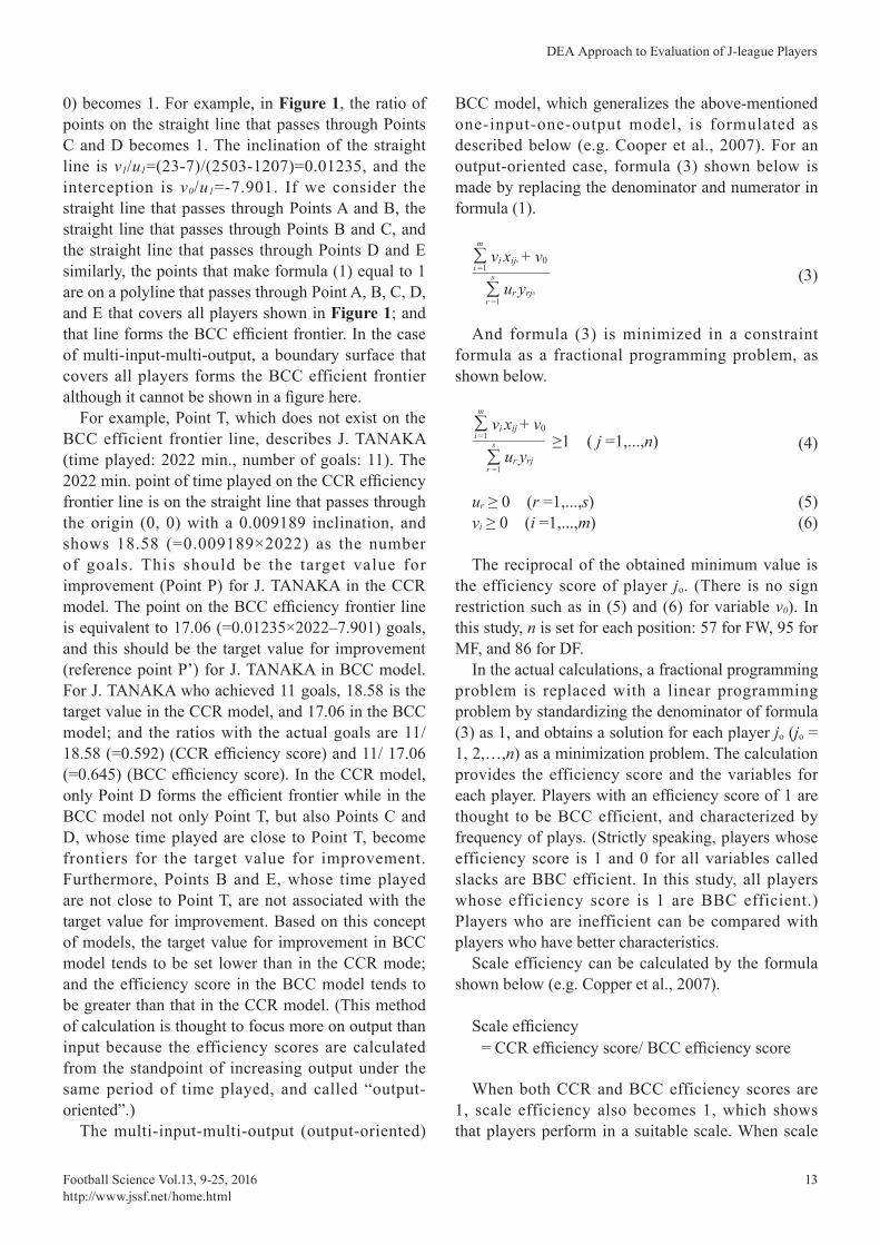
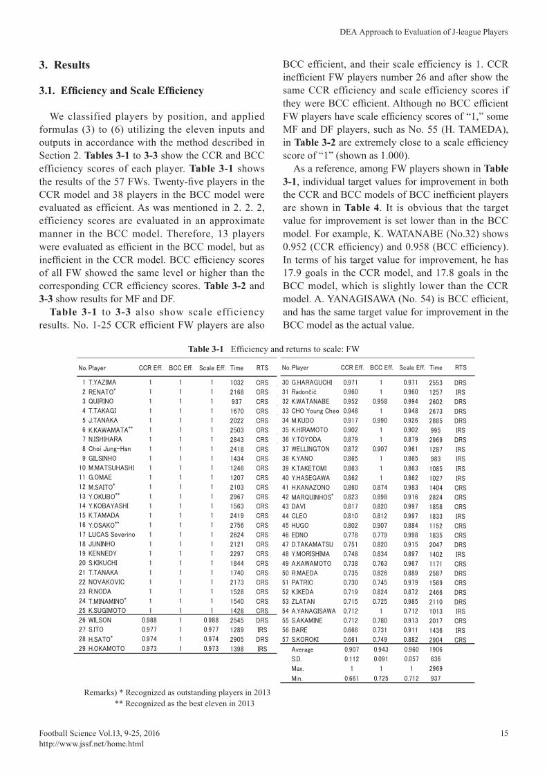
We classified players by position, and applied formulas (3) to (6) utilizing the eleven inputs and outputs in accordance with the method described in Section 2. Tables 3-1 to 3-3 show the CCR and BCC efficiency scores of each player. Table 3-1 shows the results of the 57 FWs. Twenty-five players in the CCR model and 38 players in the BCC model were evaluated as efficient. As was mentioned in 2. 2. 2, efficiency scores are evaluated in an approximate manner in the BCC model. Therefore, 13 players were evaluated as efficient in the BCC model, but as inefficient in the CCR model. BCC efficiency scores of all FW showed the same level or higher than the corresponding CCR efficiency scores. Table 3-2 and 3-3 show results for MF and DF.

Table 3-1 to 3-3 also show scale efficiency results. No. 1-25 CCR efficient FW players are also

BCC efficient, and their scale efficiency is 1. CCR inefficient FW players number 26 and after show the same CCR efficiency and scale efficiency scores if they were BCC efficient. Although no BCC efficient FW players have scale efficiency scores of “1,” some MF and DF players, such as No. 55 (H. TAMEDA), in Table 3-2 are extremely close to a scale efficiency score of “1” (shown as 1.000).

As a reference, among FW players shown in Table 3-1, individual target values for improvement in both the CCR and BCC models of BCC inefficient players are shown in Table 4. It is obvious that the target value for improvement is set lower than in the BCC model. For example, K. WATANABE (No.32) shows 0.952 (CCR efficiency) and 0.958 (BCC efficiency). In terms of his target value for improvement, he has 17.9 goals in the CCR model, and 17.8 goals in the BCC model, which is slightly lower than the CCR model. A. YANAGISAWA (No. 54) is BCC efficient, and has the same target value for improvement in the BCC model as the actual value.

Table 3-1 Efficiency and returns to scale: FW

Remarks) * Recognized as outstanding players in 2013 ** Recognized as the best eleven in 2013

No. Player CCR Eff. BCC Eff. Scale Eff. Time RTS

1 T.YAZIMA 1 1 1 1032 CRS2 RENATO* 1 1 1 2168 CRS3 QUIRINO 1 1 1 937 CRS4 T.TAKAGI 1 1 1 1670 CRS5 J.TANAKA 1 1 1 2022 CRS6 K.KAWAMATA** 1 1 1 2503 CRS7 N.ISHIHARA 1 1 1 2843 CRS8 Choi Jung-Han 1 1 1 2418 CRS9 GILSINHO 1 1 1 1434 CRS

10 M.MATSUHASHI 1 1 1 1246 CRS11 G.OMAE 1 1 1 1207 CRS12 M.SAITO* 1 1 1 2103 CRS13 Y.OKUBO** 1 1 1 2967 CRS14 Y.KOBAYASHI 1 1 1 1563 CRS15 K.TAMADA 1 1 1 2419 CRS16 Y.OSAKO** 1 1 1 2756 CRS17 LUCAS Severino 1 1 1 2624 CRS18 JUNINHO 1 1 1 2121 CRS19 KENNEDY 1 1 1 2297 CRS20 S.KIKUCHI 1 1 1 1844 CRS21 T.TANAKA 1 1 1 1740 CRS22 NOVAKOVIC 1 1 1 2173 CRS23 R.NODA 1 1 1 1528 CRS24 T.MINAMINO*: 1 1 1 1540 CRS25 K.SUGIMOTO 1 1 1 1428 CRS26 WILSON 0.988 1 0.988 2545 DRS27 S.ITO 0.977 1 0.977 1289 IRS28 H.SATO* 0.974 1 0.974 2905 DRS29 H.OKAMOTO 0.973 1 0.973 1398 IRS

30 G.HARAGUCHI 0.971 1 0.971 2553 DRS31 Radončić 0.960 1 0.960 1257 IRS32 K.WATANABE 0.952 0.958 0.994 2602 DRS33 CHO Young Cheo 0.948 1 0.948 2673 DRS34 M.KUDO 0.917 0.990 0.926 2885 DRS35 K.HIRAMOTO 0.902 1 0.902 995 IRS36 Y.TOYODA 0.879 1 0.879 2969 DRS37 WELLINGTON 0.872 0.907 0.961 1287 IRS38 K.YANO 0.865 1 0.865 983 IRS

39 K.TAKETOMI 0.863 1 0.863 1085 IRS40 Y.HASEGAWA 0.862 1 0.862 1027 IRS41 H.KANAZONO 0.860 0.874 0.983 1404 CRS42 MARQUINHOS* 0.823 0.898 0.916 2824 CRS43 DAVI 0.817 0.820 0.997 1858 CRS44 CLEO 0.810 0.812 0.997 1833 IRS45 HUGO 0.802 0.907 0.884 1152 CRS46 EDNO 0.778 0.779 0.998 1835 CRS47 D.TAKAMATSU 0.751 0.820 0.915 2047 DRS48 Y.MORISHIMA 0.748 0.834 0.897 1402 IRS49 A.KAWAMOTO 0.738 0.763 0.967 1171 CRS50 R.MAEDA 0.735 0.826 0.889 2587 DRS51 PATRIC 0.730 0.745 0.979 1569 CRS52 K.IKEDA 0.719 0.824 0.872 2466 DRS53 ZLATAN 0.715 0.725 0.985 2110 DRS54 A.YANAGISAWA 0.712 1 0.712 1013 IRS55 S.AKAMINE 0.712 0.780 0.913 2017 CRS56 BARE 0.666 0.731 0.911 1436 IRS57 S.KOROKI 0.661 0.749 0.882 2904 CRS

Average 0.907 0.943 0.960 1906

S.D. 0.112 0.091 0.057 636

Max. 1 1 1 2969

Min. 0.661 0.725 0.712 937

No. Player CCR Eff. BCC Eff. Scale Eff. Time RTS


Hirotsu, N. et al.


3.2. Super Efficiency

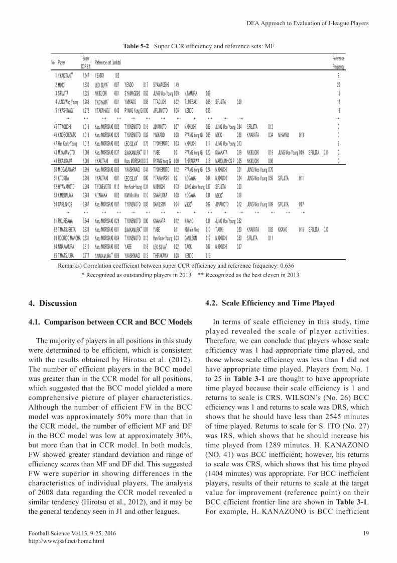
Tables 5-1 to 5-3 show super CCR efficiency results by position. Table 5-1 shows super efficiency scores of CCR efficient FW players from higher to

lower. Players No. 26 and after in Table 5-1 are CCR inefficient players. Efficient frontier does not change regardless of inclusion or exclusion of the inefficient player himself; therefore, super efficiency and CCR efficiency scores become equal. Table 5-2 and 5-3

Table 3-2 Efficiency and returns to scale: MF


49 R.KAJIKAWA 1 1 1 1166 CRS

50 M.OGASAWARA 0.999 1 0.999 2933 DRS

51 K.TOKITA 0.998 0.998 0.999 1434 IRS

52 H.YAMAMOTO 0.994 1 0.994 2554 DRS

53 K.MIZUNUMA 0.988 1 0.988 1808 IRS

54 CARLINHOS 0.987 1 0.987 989 IRS

55 H.TAMEDA 0.983 0.983 1.000 1786 DRS

56 S.TOMITA 0.980 0.980 1.000 2766 CRS

57 Y.MARUHASHI 0.977 1 0.977 2566 DRS

58 A.HASEGAWA 0.971 0.988 0.983 2797 DRS

59 R.NAGAKI 0.969 0.979 0.989 2887 DRS

60 H.OTANI 0.967 1 0.967 2770 DRS

61 Y.OTA 0.966 1 0.966 2563 DRS

62 H.ISHIGE 0.965 0.966 1.000 2131 CRS

63 S.HYODO 0.965 1 0.965 2821 DRS

64 Y.TAKAHAGI* 0.964 0.965 1.000 2744 CRS

65 Y.KAWAI 0.960 0.968 0.993 2543 DRS

66 S.KANAZAWA 0.955 0.965 0.990 2104 DRS

67 SIMPLICIO 0.949 0.951 0.999 2582 CRS

68 R.OSHIMA 0.946 1 0.946 955 IRS

69 H.TAKAHASHI 0.940 0.949 0.991 2618 DRS

70 K.HIGASHI 0.940 0.941 0.998 2594 CRS

71 K.SUZUKI 0.934 0.937 0.997 2289 CRS

72 N.FUJITA 0.933 1 0.933 2596 DRS

73 K.YAMAMOTO 0.932 0.943 0.988 1548 CRS

74 N.TAMURA 0.930 1 0.930 955 IRS

75 K.SUGIYAMA 0.927 0.998 0.929 2602 DRS

76 T.HONDA 0.921 1 0.921 1335 IRS

77 LEANDRO D 0.919 1 0.919 1031 IRS

78 T.MARUTANI 0.912 1 0.912 936 IRS

79 K.HOSAKA 0.907 0.998 0.909 1151 IRS

80 Y.KOBAYASHI 0.907 0.951 0.953 2621 DRS

81 JORGE WAGNER 0.901 0.903 0.998 1752 IRS

82 R.TAKEUCHI 0.899 0.914 0.984 1453 IRS

83 M.MIYAZAWA 0.885 0.924 0.958 1550 IRS

84 G.SHIBASAKI 0.880 0.935 0.941 2972 DRS

85 A.BARADA 0.877 0.962 0.912 1333 IRS

86 Y.KASHIWA 0.868 0.990 0.877 2934 DRS

87 T.UGAJIN 0.864 0.903 0.957 2337 DRS

88 N.SAKEMOTO 0.862 0.976 0.883 2544 DRS

89 K.MORIYA 0.860 1 0.860 902 IRS

90 H.NISHI 0.849 0.849 1.000 1570 CRS

91 R.KURISAWA 0.844 0.849 0.994 1938 CRS

92 T.MATSUSHITA 0.833 0.854 0.976 1487 IRS

93 RODRIGO MANCHA 0.831 0.853 0.974 2470 DRS

94 N.NAKAMURA 0.810 0.932 0.870 1289 IRS

95 T.MATSUURA 0.777 0.872 0.890 1318 IRS

Average 0.962 0.981 0.981 2142

S.D. 0.054 0.038 0.034 687

Max. 1 1 1 3060

Min. 0.777 0.849 0.860 902

No. Player CCR Eff. BCC Eff Scale Eff. Time RTS

1 Y.KAKITANI** 1 1 1 3018 CRS

2 MIKIC* 1 1 1 2256 CRS

3 S.FUJITA 1 1 1 950 CRS

4 JUNG Woo Young 1 1 1 967 CRS

5 Y.KASHIWAGI 1 1 1 2903 CRS

6 Kazu MORISAKI 1 1 1 2970 CRS

7 T.UMESAKI 1 1 1 1484 CRS

8 K.KANO 1 1 1 1120 CRS

9 N.KIKUCHI 1 1 1 1452 CRS

10 Y.OGAWA 1 1 1 2654 CRS

11 A.TANAKA 1 1 1 2935 CRS

12 Y.ABE* 1 1 1 2960 CRS

13 S.NAKAMURA** 1 1 1 2963 CRS

14 T.YONEMOTO 1 1 1 2764 CRS

15 LEO SILVA* 1 1 1 2812 CRS

16 S.YAMAGISHI 1 1 1 1206 CRS

17 Y.ENDO 1 1 1 1657 CRS

18 T.AOKI 1 1 1 3060 CRS

19 K.NAKATA 1 1 1 1866 CRS

20 T.HIRAKAWA 1 1 1 1906 CRS

21 KIM Min Woo 1 1 1 2932 CRS

22 RYANG Yong Gi 1 1 1 2549 CRS

23 K.NAKAMURA* 1 1 1 2532 CRS

24 J.INAMOTO 1 1 1 1758 CRS

25 MARQUINHOS P 1 1 1 1641 CRS

26 Y.MIKADO 1 1 1 2691 CRS

27 J.FUJIMOTO 1 1 1 2195 CRS

28 H.YAMADA 1 1 1 2698 CRS

29 T.AOYAMA* 1 1 1 2962 CRS

30 S.NARUOKA 1 1 1 2767 CRS

31 N.SUGAI 1 1 1 1857 CRS

32 T.AOKI 1 1 1 2440 CRS

33 H.YAMAGUCHI** 1 1 1 2926 CRS

34 T.EDAMURA 1 1 1 1048 CRS

35 Y.TAKAHASHI 1 1 1 2764 CRS

36 S.KOBAYASHI 1 1 1 2367 CRS

37 D.WATANABE 1 1 1 2849 CRS

38 T.NOZAWA 1 1 1 1553 CRS

39 R.HAYASAKA 1 1 1 1182 CRS

40 K.TAKAYAMA 1 1 1 2772 CRS

41 N.HANYU 1 1 1 1286 CRS

42 K.NAKAMACHI* 1 1 1 2903 CRS

43 DANILSON 1 1 1 2411 CRS

44 Y.KIMURA 1 1 1 1874 CRS

45 T.TAGUCHI 1 1 1 1665 CRS

46 K.NOBORIZATO 1 1 1 2517 CRS

47 Han Kook-Young 1 1 1 2634 CRS

48 M.YAMAMOTO 1 1 1 2820 CRS

No. Player CCR Eff. BCC Eff Scale Eff. Time RTS



17

show the results for MF and DF players. Super efficiency can be calculated in both CCR and

BCC models. As a reference, super efficiency scores utilizing the BCC model are also shown in Tables 6-1 to 6-3. QUIRINO (No. 38) has a super efficiency score of 1 in Table 6-1; however, his reference set players are not shown. This is because QUIRINO’s time played is 937 minutes, the shortest among the 57 FW players, making it impossible to form a reference set for QUIRINO combining other players after excluding him. (His BCC efficiency score 1 is tentatively shown as the super efficiency score.) The same is the case for K. MORIYA and T. KOBAYASHI in Tables 6-2 to 6-3.

3.3. Parameters

Results of returns to scale are shown in the RTS column in Table 3-1 to 3-3. Constant returns to scale, increasing returns to scale, and decreasing returns to scale are indicated as CRS, IRS, and DRS respectively. Results for the reference set, reference frequency, and lambda value of players in the CCR model based on the concept of super efficiency are shown in Tables 5-1 to 5-3, and those in the BCC model are shown in Tables 6-1 to 6-3 according to player position.

Table 3-3 Efficiency and returns to scale: DF


44 DUTRA* 0.997 1 0.997 2952 DRS45 T.SHIMOHIRA 0.995 1 0.995 2625 IRS46 K.OI 0.995 1 0.995 2912 DRS47 H.MIZUMOTO* 0.994 1 0.994 3060 DRS48 T.SIMAMURA 0.993 0.999 0.994 2013 DRS49 Y.TANAKA 0.987 0.992 0.995 2637 CRS50 J.KAMATA 0.982 0.990 0.992 2610 DRS51 T.IMAI 0.975 0.976 1.000 1900 IRS52 KIM Kun-Hoan 0.974 1 0.974 1630 IRS53 S.SUGANUMA 0.960 1 0.960 1437 IRS54 Y.FUJITA 0.959 0.973 0.986 2859 CRS55 Y.IGAWA 0.956 1 0.956 1092 IRS56 Y.TOKUNAGA 0.956 0.996 0.959 3060 CRS57 YEO Sung Hae 0.955 0.969 0.986 2587 CRS58 N.KAWAGUCHI 0.950 0.952 0.998 1821 IRS59 S.SASAKI 0.949 1 0.949 2970 DRS60 T.MASUKAWA 0.940 0.942 0.997 2425 CRS61 K.KIKUCHI 0.938 1 0.938 2970 DRS62 T.MURAMATSU 0.932 1 0.932 2942 DRS63 K.FUJIMOTO 0.922 0.974 0.947 2464 DRS64 T.YAMASHITA* 0.918 0.963 0.953 2223 DRS65 D.NISHI 0.918 0.935 0.982 2380 CRS66 T.SAKAI 0.916 0.998 0.919 1147 IRS67 JNAG Hyun Soo 0.907 0.909 0.998 1946 CRS68 M.INOHA 0.907 0.913 0.994 2055 CRS69 Y.KURIHARA* 0.906 0.923 0.982 2790 DRS70 Y.TSUCHIYA 0.904 0.909 0.994 1699 IRS71 N.KONDO 0.902 0.955 0.945 2790 DRS72 K.WATANABE 0.896 0.907 0.987 1694 IRS73 K.KAGA 0.894 0.973 0.919 1372 IRS74 T.MASUSHIMA 0.892 0.895 0.997 1907 DRS75 M.MORISHIGE** 0.892 0.908 0.983 2970 CRS76 H.ITO 0.892 0.949 0.940 1486 IRS77 CALVIN JONG A PIN 0.885 0.988 0.896 2340 DRS78 S.NAKAZAWA 0.869 1 0.869 1125 IRS79 S.TAKAHASHI 0.865 0.875 0.989 2854 DRS80 Y.SANETO 0.851 0.867 0.982 1679 IRS81 T.MONIWA 0.843 0.856 0.985 1342 IRS82 KIM Chang Soo 0.843 0.869 0.970 1624 IRS83 Y.YOSHIDA 0.839 0.842 0.996 2155 IRS84 S.TOMISAWA* 0.829 0.845 0.982 2502 CRS85 K.ONO 0.770 0.805 0.957 2866 DRS86 D.IWASE 0.747 0.748 0.999 1338 DRS

Average 0.958 0.972 0.986 2148

S.D. 0.059 0.052 0.026 674

Max. 1 1 1 3060

Min. 0.747 0.748 0.869 910

No. Player CCR Eff. BCC Eff Scale Eff Time RTS

1 HWANG Seok Ho 1 1 1 993 CRS2 T.OGIHARA 1 1 1 2704 CRS3 D.NASU** 1 1 1 2646 CRS4 H.TANAKA 1 1 1 3003 CRS5 K.OTA* 1 1 1 3033 CRS6 DANIEL 1 1 1 1006 CRS7 K.CHIBA 1 1 1 2992 CRS8 S.ABE 1 1 1 2700 CRS9 D.WATABE 1 1 1 1028 CRS

10 M.KAMEKAWA 1 1 1 1214 CRS11 Y.KOMANO 1 1 1 3015 CRS12 W.ENDO 1 1 1 1530 CRS13 Kim Jin-Su 1 1 1 2778 CRS14 K.HACHISUKA 1 1 1 1332 CRS15 K.YAMAMURA 1 1 1 1903 CRS16 T.MAKINO* 1 1 1 3060 CRS17 R.NIWA 1 1 1 2948 CRS18 D.SUZUKI 1 1 1 1953 CRS19 T.SHIOTANI* 1 1 1 3049 CRS20 Y.YASUKAWA 1 1 1 1922 CRS21 K.TAKAGI 1 1 1 1782 CRS22 Y.HIRAOKA 1 1 1 2670 CRS23 W.SAKATA 1 1 1 2070 CRS24 N.ISHIKAWA 1 1 1 2339 CRS25 JECI 1 1 1 1710 CRS26 T.MIYAZAKI 1 1 1 1964 CRS27 M.KAKUDA 1 1 1 2295 CRS28 LEE Kije 1 1 1 1418 CRS29 S.KAMATA 1 1 1 1699 CRS30 M.FUJITA 1 1 1 1102 CRS31 Y.NAKAZAWA** 1 1 1 3009 CRS32 MICHAEL JAMES 1 1 1 1169 CRS33 N.AOYAMA 1 1 1 2602 CRS34 T.MAENO 1 1 1 1233 CRS35 H.WATANABE 1 1 1 1056 CRS36 K.FUKUDA 1 1 1 2695 CRS37 W.HASHIMOTO 1 1 1 1608 CRS38 Marcus T.TANAKA 1 1 1 2350 CRS39 M.WAKASA 1 1 1 1572 CRS40 Y.KOBAYASHI 1 1 1 2839 CRS41 R.MORIWAKI 1 1 1 2796 CRS42 CHO Byung kuk 1 1 1 1784 CRS43 T.KOBAYASHI 0.998 1 0.998 910 IRS

No. Player CCR Eff. BCC Eff Scale Eff Time RTS


Hirotsu, N. et al.


3.4. Correlation between Reference Frequency and Super Efficiency Scores

In terms of the correlation coefficients between reference frequency and super efficiency score in the CCR model, FW was 0.630, MF was 0.636, and DF

was 0.326, as shown in Tables 5-1 to 5-3. In terms of the correlation coefficients between reference frequency and super efficiency score in the BCC model, FW was 0.414, MF was 0.574, and DF was 0.081, as is shown in Tables 6-1 to 6-3.

Table 4 Target values for improvement

Table 5-1 Super CCR efficiency and reference sets: FW

Remark) * Recognized as outstanding players in 2013

Present Target（CCR) Target(BCC)

No. Player

Goals

Asis

ts

Passes

Crosses

Drib

ble

s

Tackle

s

Intercep

tio

ns

Cle

ars

Blo

cks

Fouls

Goals

Asis

ts

Passes

Crosses

Drib

ble

s

Tackle

s

Intercep

tio

ns

Cle

ars

Blo

cks

Fouls

Goals

Asis

ts

Passes

Crosses

Drib

ble

s

Tackle

s

Intercep

tio

ns

Cle

ars

Blo

cks

Fouls

32 K.WATANABE 17 2 661 5 17 21 4 16 19 35 17.9 6.4 695 9.2 37.8 22.1 4.2 24.9 28.4 31.3 17.8 6.2 690 9.0 36.0 21.9 4.2 24.2 27.3 31.8

・・・・・・・・・・・・・・・・・・・・・・・・・・・・・・・・・・・・・・・・・・・・・・・・・・・・・・・・・・・・・・・・・・・・・・・・・・・・・・・・・・・・・・・・・・・・・34 M.KUDO 19 4 517 10 27 16 1 9 30 39 20.7 7.6 739 13.3 39.2 17.5 3.9 29.3 32.7 31.7 19.2 4.0 760 10.1 54.4 16.2 2.6 23.7 32.8 38.2

・・・・・・・・・・・・・・・・・・・・・・・・・・・・・・・・・・・・・・・・・・・・・・・・・・・・・・・・・・・・・・・・・・・・・・・・・・・・・・・・・・・・・・・・・・・・・37 WELLINGTON 3 0 279 3 6 25 1 23 19 53 3.4 2.2 320 3.4 9.3 28.7 4.3 26.4 25.3 27.1 3.3 2.4 308 3.4 12.8 27.6 3.8 26.7 24.3 35.3

・・・・・・・・・・・・・・・・・・・・・・・・・・・・・・・・・・・・・・・・・・・・・・・・・・・・・・・・・・・・・・・・・・・・・・・・・・・・・・・・・・・・・・・・・・・・・

42 MARQUINHOS* 16 3 529 11 30 25 4 5 20 79 19.4 6.6 643 13.4 38.3 30.4 4.9 31.3 28.7 45.0 17.8 6.5 818 12.2 53.1 27.8 4.45 13.7 33.2 48.2

・・・・・・・・・・・・・・・・・・・・・・・・・・・・・・・・・・・・・・・・・・・・・・・・・・・・・・・・・・・・・・・・・・・・・・・・・・・・・・・・・・・・・・・・・・・・・

53 ZLATAN 6 1 552 14 27 17 3 10 18 52 8.6 9.5 773 21.6 54.7 29.0 4.2 14.0 32.6 38.1 8.9 7.6 761 19.3 50.3 31.8 4.1 13.8 30.2 38.854 A.YANAGISAWA 3 1 195 0 1 8 0 0 8 18 4.2 2.7 317 6.1 12.0 11.2 2.2 9.4 14.4 8.4 3.0 1.0 195 0.0 1.0 8.0 0.0 0.0 8.0 18.055 S.AKAMINE 3 4 424 5 7 13 1 32 16 45 4.9 5.6 595 13.6 23.1 32.3 2.8 44.9 44.8 29.6 6.2 5.1 543 16.3 31.2 28.4 4.0 41.0 33.0 27.756 BARE 4 1 171 9 22 10 0 16 9 34 6.0 3.5 348 13.5 33.1 15.4 1.6 24.0 20.1 20.3 5.5 4.4 368 12.3 30.1 18.6 3.1 21.9 27.1 24.757 S.KOROKI 13 5 607 6 19 10 1 14 11 75 19.7 7.6 919 16.7 65.5 25.5 2.9 21.2 39.4 46.6 17.4 6.7 811 14.5 50.1 22.2 3.0 18.7 31.8 50.5

Remarks) Correlation coefficient between super CCR efficiency and reference frequency: 0.630 * Recognized as outstanding players in 2013 ** Recognized as the best eleven in 2013

No. PlayerSuperCCR Eff.

Reference set (lambda)ReferenceFrequency

1 T.YAZIMA 1.695 N.ISHIHARA 0.36 52 RENATO* 1.621 Y.OKUBO** 0.09 M.SAITO* 0.71 J.TANAKA 0.19 15

3 QUIRINO 1.482 K.KAWAMATA** 0.00 Choi Jung-Han 0.04 KENNEDY 0.10 Radončić 0.01 M.MATSUHASHI 0.48 22

4 T.TAKAGI 1.408 RENATO* 0.54 T.YAZIMA 0.49 3

5 J.TANAKA 1.395 NOVAKOVIC 0.09 RENATO* 0.49 T.TAKAGI 0.29 QUIRINO 0.29 18・・・・・・・・・・・・・・・・・・・・・・・・・・・・・・・・・

21 T.TANAKA 1.027 K.TAMADA 0.15 J.TANAKA 0.34 GILSINHO 0.33 T.YAZIMA 0.21 022 NOVAKOVIC 1.026 K.KAWAMATA** 0.41 Choi Jung-Han 0.02 J.TANAKA 0.20 M.MATSUHASHI 0.56 1

23 R.NODA 1.016 RENATO 0.12 M.SAITO* 0.23 GILSINHO 0.03 M.MATSUHASHI 0.03 T.YAZIMA 0.10 QUIRINO 0.65 0

24 T.MINAMINO*: 1.009 K.TAMADA 0.00 RENATO 0.11 J.TANAKA 0.34 Y.KOBAYASHI 0.20 M.MATSUHASHI 0.24 025 K.SUGIMOTO 1.008 RENATO 0.28 M.MATSUHASHI 0.53 QUIRINO 0.17 0

26 WILSON 0.988 Y.OKUBO** 0.30 JUNINHO 0.28 J.TANAKA 0.21 T.TAKAGI 0.3827 S.ITO 0.977 J.TANAKA 0.51 M.MATSUHASHI 0.03 G.OMAE 0.01 QUIRINO 0.2128 H.SATO* 0.974 Y.OSAKO 0.10 K.KAWAMATA** 0.13 J.TANAKA 1.1329 H.OKAMOTO 0.973 N.ISHIHARA 0.02 J.TANAKA 0.39 Y.KOBAYASHI 0.17 T.YAZIMA 0.2930 G.HARAGUCHI 0.971 RENATO* 0.25 JUNINHO 0.12 J.TANAKA 0.44 T.TAKAGI 0.52

・・・・・・・・・・・・・・・・・・・・・・・・・・・・・・42 MARQUINHOS* 0.823 Y.OKUBO** 0.10 N.ISHIHARA 0.27 Y.OSAKO** 0.06 K.KAWAMATA 0.46 RENATO* 0.20

・・・・・・・・・・・・・・・・・・・・・・・・・・・・・・

53 ZLATAN 0.715 RENATO* 0.50 J.TANAKA 0.24 GILSINHO 0.32 M.MATSUHASHI 0.0754 A.YANAGISAWA 0.712 K.TAMADA 0.10 J.TANAKA 0.19 Y.KOBAYASHI 0.2555 S.AKAMINE 0.712 RENATO

* 0.12 J.TANAKA 0.28 M.MATSUHASH 0.83 QUIRINO 0.1456 BARE 0 666 K KAWAMATA** 0 16 Choi Jung-Han 0 26 RENATO* 0 16 QUIRINO 0 0757 S.KOROKI 0.661 Y.OKUBO** 0.50 LUCAS Severino 0.11 RENATO* 0.42 QUIRINO 0.24



19

4. Discussion

4.1. Comparison between CCR and BCC Models

The majority of players in all positions in this study were determined to be efficient, which is consistent with the results obtained by Hirotsu et al. (2012). The number of efficient players in the BCC model was greater than in the CCR model for all positions, which suggested that the BCC model yielded a more comprehensive picture of player characteristics. Although the number of efficient FW in the BCC model was approximately 50% more than that in the CCR model, the number of efficient MF and DF in the BCC model was low at approximately 30%, but more than that in CCR model. In both models, FW showed greater standard deviation and range of efficiency scores than MF and DF did. This suggested FW were superior in showing differences in the characteristics of individual players. The analysis of 2008 data regarding the CCR model revealed a similar tendency (Hirotsu et al., 2012), and it may be the general tendency seen in J1 and other leagues.

4.2. Scale Efficiency and Time Played

In terms of scale efficiency in this study, time played revealed the scale of player activities. Therefore, we can conclude that players whose scale efficiency was 1 had appropriate time played, and those whose scale efficiency was less than 1 did not have appropriate time played. Players from No. 1 to 25 in Table 3-1 are thought to have appropriate time played because their scale efficiency is 1 and returns to scale is CRS. WILSON’s (No. 26) BCC efficiency was 1 and returns to scale was DRS, which shows that he should have less than 2545 minutes of time played. Returns to scale for S. ITO (No. 27) was IRS, which shows that he should increase his time played from 1289 minutes. H. KANAZONO (NO. 41) was BCC inefficient; however, his returns to scale was CRS, which shows that his time played (1404 minutes) was appropriate. For BCC inefficient players, results of their returns to scale at the target value for improvement (reference point) on their BCC efficient frontier line are shown in Table 3-1. For example, H. KANAZONO is BCC inefficient

Table 5-2 Super CCR efficiency and reference sets: MF

Remarks) Correlation coefficient between super CCR efficiency and reference frequency: 0.636* Recognized as outstanding players in 2013 ** Recognized as the best eleven in 2013

No. PlayerSuper

CCR Eff.Reference set (lambda)

ReferenceFrequency

1 Y.KAKITANI** 1.647 Y.ENDO 1.82 9

2 MIKIC* 1.630 LEO SILVA* 0.07 Y.ENDO 0.17 S.YAMAGISHI 1.49 203 S.FUJITA 1.325 N.KIKUCHI 0.01 S.YAMAGISHI 0.63 JUNG Woo Young 0.09 N.TAMURA 0.09 154 JUNG Woo Young 1.286 T.AOYAMA* 0.01 Y.MIKADO 0.08 T.TAGUCHI 0.32 T.UMESAKI 0.06 S.FUJITA 0.09 125 Y.KASHIWAGI 1.272 Y.TAKAHAGI 0.43 RYANG Yong Gi 0.00 J.FUJIMOTO 0.36 Y.ENDO 0.56 16

・・・・・・・・・・・・・・・・・・・・・・・・・・・・・・・・・・・・・・・45 T.TAGUCHI 1.016 Kazu MORISAKI 0.02 T.YONEMOTO 0.16 J.INAMOTO 0.07 N.KIKUCHI 0.09 JUNG Woo Young 0.84 S.FUJITA 0.12 046 K.NOBORIZATO 1.016 Kazu MORISAKI 0.20 T.YONEMOTO 0.02 Y.MIKADO 0.08 RYANG Yong Gi 0.05 MIKIC 0.28 K.NAKATA 0.34 N.HANYU 0.19 047 Han Kook-Young 1.012 Kazu MORISAKI 0.02 LEO SILVA* 0.75 T.YONEMOTO 0.03 N.KIKUCHI 0.17 JUNG Woo Young 0.13 2

48 M.YAMAMOTO 1.008 Kazu MORISAKI 0.37 S.NAKAMURA** 0.11 Y.ABE 0.01 RYANG Yong Gi 0.20 K.NAKATA 0.19 N.KIKUCHI 0.19 JUNG Woo Young 0.09 S.FUJITA 0.11 049 R.KAJIKAWA 1.006 Y.KAKITANI 0.09 Kazu MORISAKI 0.12 RYANG Yong Gi 0.00 T.HIRAKAWA 0.18 MARQUINHOS P 0.05 N.KIKUCHI 0.06 050 M.OGASAWARA 0.999 Kazu MORISAKI 0.03 Y.KASHIWAGI 0.41 T.YONEMOTO 0.12 RYANG Yong Gi 0.24 N.KIKUCHI 0.01 JUNG Woo Young 0.7051 K.TOKITA 0.998 Y.KAKITANI 0.01 LEO SILVA* 0.00 Y.TAKAHASHI 0.21 Y.OGAWA 0.04 N.KIKUCHI 0.04 JUNG Woo Young 0.59 S.FUJITA 0.1152 H.YAMAMOTO 0.994 T.YONEMOTO 0.12 Han Kook-Young 0.31 N.KIKUCHI 0.73 JUNG Woo Young 0.37 S.FUJITA 0.0053 K.MIZUNUMA 0.988 A.TANAKA 0.02 KIM Min Woo 0.10 S.NARUOKA 0.08 Y.OGAWA 0.31 MIKIC* 0.18

54 CARLINHOS 0.987 Kazu MORISAKI 0.07 T.YONEMOTO 0.03 DANILSON 0.04 MIKIC* 0.09 J.INAMOTO 0.12 JUNG Woo Young 0.09 S.FUJITA 0.07・・・・・・・・・・・・・・・・・・・・・・・・・・・・・・・・・・・・・・・・・・・・・・・・

91 R.KURISAWA 0.844 Kazu MORISAKI 0.29 T.YONEMOTO 0.00 K.NAKATA 0.12 K.KANO 0.31 JUNG Woo Young 0.5292 T.MATSUSHITA 0.833 Kazu MORISAKI 0.01 S.NAKAMURA** 0.01 Y.ABE 0.11 KIM Min Woo 0.10 T.AOKI 0.20 K.NAKATA 0.02 K.KANO 0.16 S.FUJITA 0.1093 RODRIGO MANCHA 0.831 Kazu MORISAKI 0.04 T.YONEMOTO 0.13 Han Kook-Young 0.33 DANILSON 0.12 N.KIKUCHI 0.50 S.FUJITA 0.1194 N.NAKAMURA 0.810 Kazu MORISAKI 0.02 Y.ABE 0.16 LEO SILVA* 0.22 T.AOKI 0.02 N.KIKUCHI 0.07

95 T.MATSUURA 0.777 S.NAKAMURA** 0.06 Y.KASHIWAGI 0.13 T.HIRAKAWA 0.28 Y.ENDO 0.13


Hirotsu, N. et al.


Table 5-3 Super CCR efficiency and reference sets: DF

Table 6-1 Super BCC efficiency and reference sets: FW

Remarks) Correlation coefficient between super BCC efficiency and reference frequency: 0.414 * Recognized as outstanding players in 2013 ** Recognized as the best eleven in 2013

No. PlayerSuper

BCC Eff.Reference set (lambda)

ReferenceFrequency

1 T.YAZIMA 2.424 GILSINHO 0.08 G.OMAE 0.05 K.YANO 0.86 1

2 N.ISHIHARA 1.919 LUCAS Severino 0.11 KENNEDY 0.89 8

3 RENATO* 1.622 Y.OKUBO** 0.09 M.SAITO* 0.71 J.TANAKA 0.19 11

4 Choi Jung-Han 1.546 LUCAS Severino 0.63 JUNINHO 0.35 QUIRINO 0.02 7

5 Y.OKUBO** 1.413 M.KUDO 0.16 Y.OSAKO 0.76 RENATO* 0.09 10

・・・・・・・・・・・・・・・・・・・・・・・・・・・

34 G.HARAGUCHI 1.018 Y.OKUBO** 0.35 N.ISHIHARA 0.01 CHO Young Cheol 0.15 Choi Jung-Han 0.28 JUNINHO 0.05 M.SAITO* 0.07 J.TANAKA 0.01 T.TAKAGI 0.08 0

35 WILSON 1.017 Y.OKUBO** 0.38 Choi Jung-Han 0.39 RENATO* 0.06 J.TANAKA 0.16 0

36 K.SUGIMOTO 1.010 RENATO* 0.26 GILSINHO 0.06 M.MATSUHASHI 0.47 QUIRINO 0.21 0

37 H.OKAMOTO 1.010 J.TANAKA 0.22 Y.KOBAYASHI 0.17 S.ITO 0.16 G.OMAE 0.09 T.YAZIMA 0.36 0

38 QUIRINO 1.000 12

39 M.KUDO 0.990 Y.OKUBO** 0.67 H.SATO* 0.00 Y.OSAKO 0.06 Choi Jung-Han 0.24 RENATO* 0.03

40 K.WATANABE 0.958 Y.OKUBO** 0.29 H.SATO* 0.00 N.ISHIHARA 0.06 Y.OSAKO** 0.31 K.TAMADA 0.05 J.TANAKA 0.28

41 HUGO 0.907 Y.OKUBO** 0.03 K.KAWAMATA** 0.01 G.OMAE 0.52 QUIRINO 0.44

42 WELLINGTON 0.907 N.ISHIHARA 0.15 GILSINHO 0.09 K.HIRAMOTO 0.26 QUIRINO 0.50

43 MARQUINHOS* 0.898 Y.OKUBO** 0.43 N.ISHIHARA 0.22 Y.OSAKO** 0.03 RENATO* 0.32

44 H.KANAZONO 0.874 N.ISHIHARA 0.04 Y.OSAKO** 0.17 G.OMAE 0.35 QUIRINO 0.45

・・・・・・・・・・・・・・・・・・・・・・・・・・・・・・

53 A.KAWAMOTO 0.763 RENATO* 0.02 GILSINHO 0.40 M.MATSUHASHI 0.02 QUIRINO 0.55

54 S.KOROKI 0.749 Y.OKUBO** 0.41 LUCAS Severino 0.21 RENATO* 0.25 J.TANAKA 0.13

55 PATRIC 0.745 K.KAWAMATA 0.20 RENATO* 0.20 G.OMAE 0.20 T.YAZIMA 0.08 QUIRINO 0.31

56 BARE 0.731 Choi Jung-Han 0.03 RENATO* 0.19 J.TANAKA 0.03 T.TAKAGI 0.19 S.ITO 0.15 QUIRINO 0.42

57 ZLATAN 0.725 N.ISHIHARA 0.05 LUCAS Severino 0.13 K.TAMADA 0.06 RENATO* 0.46 J.TANAKA 0.06 GILSINHO 0.22

Remarks) Correlation coefficient between super CCR efficiency and reference frequency: 0.326 * Recognized as outstanding players in 2013 ** Recognized as the best eleven in 2013

No. PlayerSuper

CCR Eff.Reference set (lambda)

ReferenceFrequency

1 HWANG Seok Ho 1.729 T.MAKINO* 0.14 Y.KOMANO 0.13 D.NASU** 0.07 2

2 T.OGIHARA 1.700 K.OTA* 0.38 R.NIWA 0.29 R.MORIWAKI 0.25 11

3 D.NASU** 1.521 T.MAKINO* 0.55 M.KAKUDA 0.15 HWANG Seok Ho 0.62 134 H.TANAKA 1.489 K.OTA 0.04 W.HASHIMOTO 1.37 M.KAMEKAWA 0.56 45 K.OTA* 1.427 Y.KOMANO 0.79 T.OGIHARA 0.23 HWANG Seok Ho 0.02 3

・・・・・・・・・・・・・・・・・・・・・・・・39 M.WAKASA 1.016 Kim Jin-Su 0.00 D.NASU** 0.05 Y.YASUKAWA 0.74 HWANG Seok Ho 0.00 140 Y.KOBAYASHI 1.010 Y.KOMANO 0.40 S.ABE 0.25 T.MIYAZAKI 0.17 S.KAMATA 0.20 D.WATABE 0.28 041 R.MORIWAKI 1.010 T.MAKINO* 0.09 T.OGIHARA 0.28 D.NASU** 0.35 K.HACHISUKA 0.33 M.KAMEKAWA 0.33 0

42 CHO Byung kuk 1.003 T.SHIOTANI* 0.18 Kim Jin-Su 0.00 T.OGIHARA 0.15 Y.YASUKAWA 0.40 DANIEL 0.06 0

43 T.KOBAYASHI 0.998 N.AOYAMA 0.10 JECI 0.27 DANIEL 0.1944 DUTRA* 0.997 Y.KOMANO 0.18 K.CHIBA 0.03 S.ABE 0.35 N.ISHIKAWA 0.01 T.MIYAZAKI 0.31 S.KAMATA 0.02 M.KAMEKAWA 0.59

45 T.SHIMOHIRA 0.995 T.SHIOTANI* 0.35 K.OTA* 0.09 Kim Jin-Su 0.46

46 K.OI 0.995 T.SHIOTANI* 0.05 D.NASU** 0.03 W.SAKATA 0.34 JECI 0.19 D.WATABE 1.29 DANIEL 0.33

47 H.MIZUMOTO* 0.994 K.CHIBA 0.22 S.ABE 0.06 S.KAMATA 0.23 W.ENDO 0.74 M.KAMEKAWA 0.58・・・・・・・・・・・・・・・・・・・・・・・・・・・・・・・・・・・・

82 KIM Chang Soo 0.843 Y.KOMANO 0.06 H.TANAKA 0.07 R.NIWA 0.02 Kim Jin-Su 0.13 S.ABE 0.21 W.SAKATA 0.09 D.SUZUKI 0.01 K.YAMAMURA 0.0083 Y.YOSHIDA 0.839 T.SHIOTANI* 0.00 Y.KOMANO 0.16 H.TANAKA 0.12 R.NIWA 0.16 Kim Jin-Su 0.02 T.OGIHARA 0.05 S.ABE 0.18 D.NASU** 0.05 D.SUZUKI 0.01

84 S.TOMISAWA* 0.829 T.SHIOTANI* 0.36 K.OTA* 0.01 K.CHIBA 0.02 T.OGIHARA 0.01 D.NASU** 0.24 W.ENDO 0.12 D.WATABE 0.47

85 K.ONO 0.770 D.NASU** 0.21 N.ISHIKAWA 0.07 W.SAKATA 0.63 JECI 0.17 D.WATABE 0.5386 D.IWASE 0.747 T.OGIHARA 0.18 LEE Kije 0.00 MICHAEL JAMES 0.05 DANIEL 0.80



21

Table 6-2 Super BCC efficiency and reference sets: MF

Table 6-3 Super BCC efficiency and reference sets: DF


No. PlayerSuperBCC Eff.

Reference set (lambda)ReferenceFrequency

1 S.FUJITA 2.819 S.YAMAGISHI 0.03 N.TAMURA 0.69 R.OSHIMA 0.01 K.MORIYA 0.26 92 Y.KAKITANI** 2.100 S.NAKAMURA** 1.00 53 MIKIC* 1.946 S.NAKAMURA** 0.45 S.KOBAYASHI 0.22 S.YAMAGISHI 0.33 124 JUNG Woo Young 1.784 T.EDAMURA 0.25 CARLINHOS 0.12 N.TAMURA 0.13 S.FUJITA 0.22 K.MORIYA 0.27 135 T.AOKI 1.703 Y.ABE 0.14 K.TAKAYAMA 0.09 H.YAMAMOTO 0.77 8

・・・・・・・・・・・・・・・・・・・・・・・・・・・

60 K.MIZUNUMA 1.018 Y.OGAWA 0.36 MIKIC* 0.16 Y.ENDO 0.03 K.KANO 0.09 JUNG Woo Young 0.19 S.FUJITA 0.17 061 Y.KIMURA 1.018 T.YONEMOTO 0.01 RYANG Yong Gi 0.02 J.FUJIMOTO 0.65 K.NAKATA 0.07 K.KANO 0.01 JUNG Woo Young 0.19 S.FUJITA 0.06 162 Han Kook-Young 1.013 T.AOKI 0.00 Kazu MORISAKI 0.01 T.AOYAMA* 0.06 LEO SILVA* 0.74 H.YAMAMOTO 0.07 N.KIKUCHI 0.12 JUNG Woo Young 0.01 363 N.FUJITA 1.008 T.AOKI 0.01 Y.KASHIWAGI 0.22 H.OTANI 0.23 T.YONEMOTO 0.22 Y.TAKAHASHI 0.16 T.TAGUCHI 0.10 JUNG Woo Young 0.05 064 K.MORIYA 1.000 1

65 K.SUGIYAMA 0.998 T.AOKI 0.19 Y.TAKAHASHI 0.51 Han Kook-Young 0.11 H.YAMAMOTO 0.05 N.KIKUCHI 0.15

66 K.TOKITA 0.998 Y.KAKITANI** 0.01 H.YAMAGUCHI** 0.00 T.YONEMOTO 0.00 Y.TAKAHASHI 0.20 Y.OGAWA 0.03 N.KIKUCHI 0.04 JUNG Woo Young 0.60 S.FUJITA 0.112

67 K.HOSAKA 0.998 Y.KAKITANI** 0.01 T.AOKI 0.05 N.KIKUCHI 0.08 R.KAJIKAWA 0.09 K.KANO 0.18 JUNG Woo Young 0.17 R.OSHIMA 0.41

68 Y.KASHIWA 0.990 T.AOKI 0.03 S.NAKAMURA** 0.05 H.YAMAGUCHI** 0.28 Y.KASHIWAGI 0.10 LEO SILVA* 0.08 MIKIC* 0.45

69 A.HASEGAWA 0.988 H.YAMAGUCHI** 0.05 Y.KASHIWAGI 0.82 M.YAMAMOTO 0.03 K.TAKAYAMA 0.04 N.KIKUCHI 0.07

・・・・・・・・・・・・・・・・・・・・・・・・・・・・・・・・・

91 T.MATSUURA 0.872 T.HIRAKAWA 0.20 Y.ENDO 0.20 T.UMESAKI 0.00 S.YAMAGISHI 0.01 LEANDRO D 0.45 R.OSHIMA 0.14

92 T.MATSUSHITA 0.854 Kazu MORISAKI 0.08 LEO SILVA* 0.01 T.AOKI 0.11 Y.ENDO 0.21 K.KANO 0.20 JUNG Woo Young 0.28 R.OSHIMA 0.01 S.FUJITA 0.092

93 RODRIGO MANCHA 0.853 T.AOKI 0.02 Kazu MORISAKI 0.02 T.YONEMOTO 0.01 Y.TAKAHASHI 0.05 Han Kook-Young 0.31 H.YAMAMOTO 0.32 K.NOBORIZATO 0.09 K.NAKATA 0.19

94 H.NISHI 0.849 H.YAMAGUCHI** 0.07 MIKIC* 0.12 MARQUINHOS P 0.16 N.HANYU 0.65

95 R.KURISAWA 0.849 Kazu MORISAKI 0.25 KIM Min Woo 0.00 K.NAKAMACHI* 0.15 MIKIC* 0.00 K.NAKATA 0.19 K.KANO 0.06 JUNG Woo Young 0.35


No. DMUSuper

BCC Eff.Reference set (lambda)

ReferenceFrequency

1 HWANG Seok Ho 6.138 M.FUJITA 0.19 DANIEL 0.49 T.KOBAYASHI 0.32 1

2 M.KAMEKAWA 1.773 R.NIWA 0.04 T.MAENO 0.44 H.WATANABE 0.52 4

3 T.OGIHARA 1.705 K.OTA* 0.37 R.NIWA 0.28 R.MORIWAKI 0.20 T.MAENO 0.14 9

4 D.NASU** 1.649 T.MAKINO* 0.46 M.KAKUDA 0.54 9

5 Y.KOMANO 1.619 T.MAKINO* 0.55 K.OTA* 0.44 HWANG Seok Ho 0.02 10

・・・・・・・・・・・・・・・・・・・・・・・・・・・・・・

50 S.SUGANUMA 1.006 K.CHIBA 0.07 S.KAMATA 0.06 W.ENDO 0.39 M.KAMEKAWA 0.16 D.WATABE 0.32 0

51 Y.IGAWA 1.005 T.SHIOTANI* 0.01 K.CHIBA 0.03 H.WATANABE 0.16 DANIEL 0.80 0

52 KIM Kun-Hoan 1.003 K.CHIBA 0.01 N.ISHIKAWA 0.31 D.SUZUKI 0.02 W.ENDO 0.33 M.KAMEKAWA 0.01 D.WATABE 0.28 DANIEL 0.04 0

53 T.SHIMOHIRA 1.001 T.SHIOTANI* 0.32 K.OTA* 0.12 Kim Jin-Su 0.40 H.WATANABE 0.12 D.WATABE 0.04 0

54 T.KOBAYASHI 1.000 4

55 T.SIMAMURA 0.999 Y.KOMANO 0.02 S.ABE 0.01 Y.HIRAOKA 0.08 N.AOYAMA 0.39 K.TAKAGI 0.09 JECI 0.18 DANIEL 0.23

56 T.SAKAI 0.998 S.KAMATA 0.21 D.WATABE 0.62 T.KOBAYASHI 0.18

57 Y.TOKUNAGA 0.996 T.SHIOTANI* 0.16 Y.KOMANO 0.30 Y.NAKAZAWA 0.34 S.ABE 0.19

58 Y.TANAKA 0.992 K.OTA* 0.28 Kim Jin-Su 0.22 T.OGIHARA 0.27 Y.HIRAOKA 0.09 Y.YASUKAWA 0.07 D.WATABE 0.04 DANIEL 0.03

59 J.KAMATA 0.990 T.SHIOTANI* 0.40 K.OI 0.02 Kim Jin-Su 0.38 W.SAKATA 0.06 DANIEL 0.13

・・・・・・・・・・・・・・・・・・・・・・・・・・・・・・・・・・・・・・・

82 T.MONIWA 0.856 N.ISHIKAWA 0.16 W.SAKATA 0.14 D.WATABE 0.05 DANIEL 0.43 T.KOBAYASHI 0.22

83 S.TOMISAWA* 0.845 T.SHIOTANI* 0.32 K.OTA* 0.10 Kim Jin-Su 0.05 T.OGIHARA 0.00 S.ABE 0.08 D.NASU** 0.25 D.WATABE 0.20

84 Y.YOSHIDA 0.842 T.SHIOTANI* 0.03 Y.KOMANO 0.11 H.TANAKA 0.14 Kim Jin-Su 0.06 S.ABE 0.17 D.NASU** 0.05 D.SUZUKI 0.01 W.HASHIMOTO 0.04 T.MAENO 0.11 M.KAMEKAWA 0.28

85 K.ONO 0.805 K.OI 0.55 Kim Jin-Su 0.01 S.ABE 0.03 Y.HIRAOKA 0.28 D.NASU** 0.14

86 D.IWASE 0.748 T.OGIHARA 0.18 K.TAKAGI 0.02 W.ENDO 0.00 LEE Kije 0.02 DANIEL 0.78


Hirotsu, N. et al.


and needs to increase efficiency to the target value for improvement. His returns to scale at the target value for improvement (reference point) are CRS, and his time played is appropriate. Returns to scale of K. WATANABE (No. 32) at his target value for improvement (reference point) is DRS, indicating that it is more efficient to decrease his time played. Application of the DEA method as described above allows us to discuss player characteristics from the standpoint of scale efficiency.

In this study, players did not increase meaningless passes or dribbles during games. We used data on frequency acquired while players were playing to win. Therefore, it is necessary to understand that target values for improvement were not set to increase meaningless plays for improvement in frequency, but simply to improve their play naturally during games.

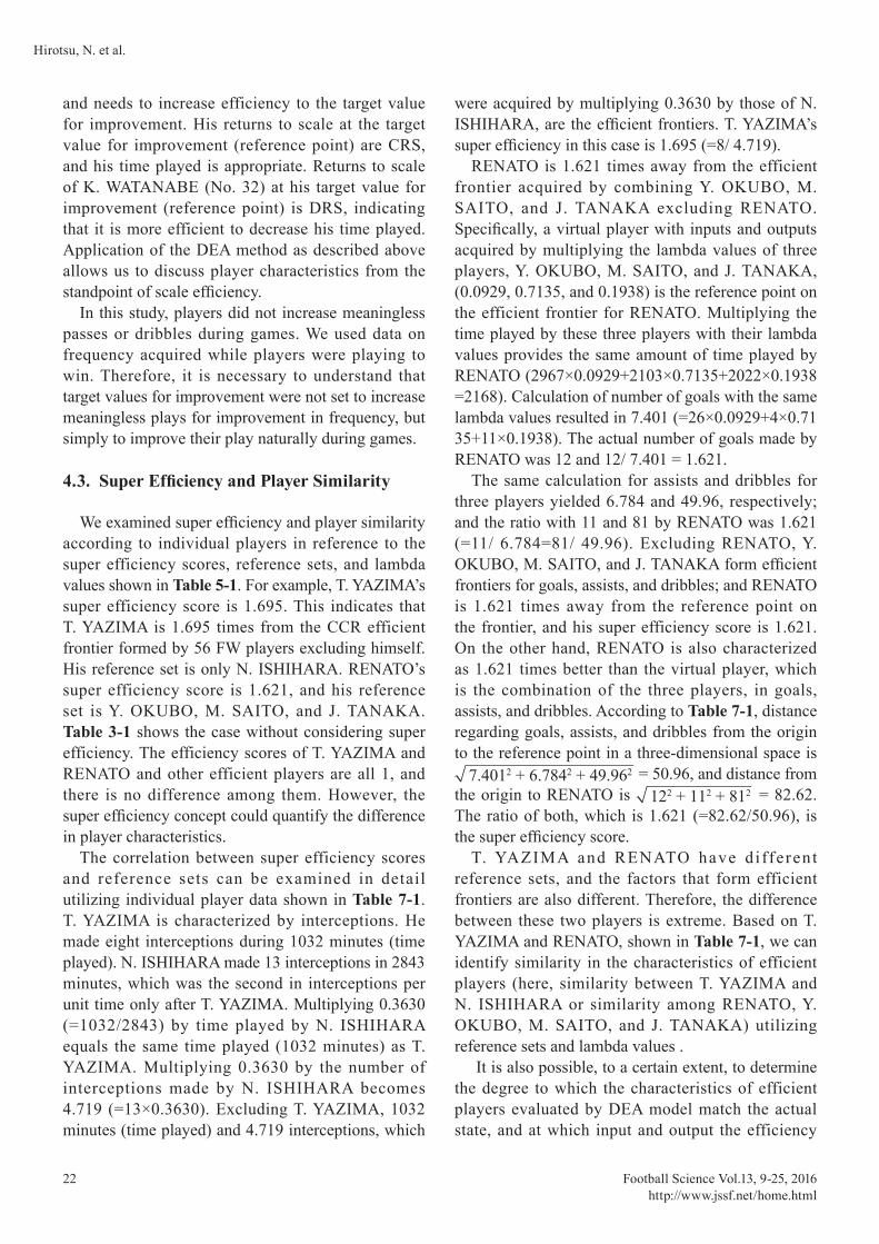
4.3. Super Efficiency and Player Similarity

We examined super efficiency and player similarity according to individual players in reference to the super efficiency scores, reference sets, and lambda values shown in Table 5-1. For example, T. YAZIMA’s super efficiency score is 1.695. This indicates that T. YAZIMA is 1.695 times from the CCR efficient frontier formed by 56 FW players excluding himself. His reference set is only N. ISHIHARA. RENATO’s super efficiency score is 1.621, and his reference set is Y. OKUBO, M. SAITO, and J. TANAKA. Table 3-1 shows the case without considering super efficiency. The efficiency scores of T. YAZIMA and RENATO and other efficient players are all 1, and there is no difference among them. However, the super efficiency concept could quantify the difference in player characteristics.

The correlation between super efficiency scores and reference sets can be examined in detail utilizing individual player data shown in Table 7-1. T. YAZIMA is characterized by interceptions. He made eight interceptions during 1032 minutes (time played). N. ISHIHARA made 13 interceptions in 2843 minutes, which was the second in interceptions per unit time only after T. YAZIMA. Multiplying 0.3630 (=1032/2843) by time played by N. ISHIHARA equals the same time played (1032 minutes) as T. YAZIMA. Multiplying 0.3630 by the number of interceptions made by N. ISHIHARA becomes 4.719 (=13×0.3630). Excluding T. YAZIMA, 1032 minutes (time played) and 4.719 interceptions, which

were acquired by multiplying 0.3630 by those of N. ISHIHARA, are the efficient frontiers. T. YAZIMA’s super efficiency in this case is 1.695 (=8/ 4.719).

RENATO is 1.621 times away from the efficient frontier acquired by combining Y. OKUBO, M. SAITO, and J. TANAKA excluding RENATO. Specifically, a virtual player with inputs and outputs acquired by multiplying the lambda values of three players, Y. OKUBO, M. SAITO, and J. TANAKA, (0.0929, 0.7135, and 0.1938) is the reference point on the efficient frontier for RENATO. Multiplying the time played by these three players with their lambda values provides the same amount of time played by RENATO (2967×0.0929+2103×0.7135+2022×0.1938=2168). Calculation of number of goals with the same lambda values resulted in 7.401 (=26×0.0929+4×0.7135+11×0.1938). The actual number of goals made by RENATO was 12 and 12/ 7.401 = 1.621.

The same calculation for assists and dribbles for three players yielded 6.784 and 49.96, respectively; and the ratio with 11 and 81 by RENATO was 1.621 (=11/ 6.784=81/ 49.96). Excluding RENATO, Y. OKUBO, M. SAITO, and J. TANAKA form efficient frontiers for goals, assists, and dribbles; and RENATO is 1.621 times away from the reference point on the frontier, and his super efficiency score is 1.621. On the other hand, RENATO is also characterized as 1.621 times better than the virtual player, which is the combination of the three players, in goals, assists, and dribbles. According to Table 7-1, distance regarding goals, assists, and dribbles from the origin to the reference point in a three-dimensional space is

7.4012 + 6.7842 + 49.962 = 50.96, and distance from the origin to RENATO is 122 + 112 + 812 = 82.62. The ratio of both, which is 1.621 (=82.62/50.96), is the super efficiency score.

T. YAZIMA and RENATO have d i ffe rent reference sets, and the factors that form efficient frontiers are also different. Therefore, the difference between these two players is extreme. Based on T. YAZIMA and RENATO, shown in Table 7-1, we can identify similarity in the characteristics of efficient players (here, similarity between T. YAZIMA and N. ISHIHARA or similarity among RENATO, Y. OKUBO, M. SAITO, and J. TANAKA) utilizing reference sets and lambda values .

It is also possible, to a certain extent, to determine the degree to which the characteristics of efficient players evaluated by DEA model match the actual state, and at which input and output the efficiency



23

score 1 is acquired utilizing each value in the

weighted output r =1

ur yrjo

s∑ (Hirotsu et al., 2012). Table

7-2 shows the data for T. YAZIMA and RENATO. These values show the ratio of the contribution of each input and output to bring the efficiency score to 1, which makes it possible to identify player characteristics and correlation with actual frequency.

As is shown in Table 7-2, for example, T YAZIMA only excels in interceptions with a super efficiency score of 1.695. This proves that he was evaluated by the number of interceptions per time played, as was mentioned above. Ranking second in interceptions, N. ISHIHARA’s goals, tackles and interceptions are 0.18, 0.58, and 0.24, respectively, indicating that he is efficient, and made many tackles. In fact, N. ISHIHARA was ranked top among FW players at 67 tackles for the year.

When RENATO’s goals, assists, and dribbles against time played were 0.18, 0.25, and 0.57, respectively, his characteristics were very distinctive. RENATO was characterized by frequency exceeding the virtual player who made the same number of goals Y. OKUBO scored, assists that J. TANAKA made, and dribbles M. SAITO made. In addition, RENATO was ranked top among FW players at 11 assists and

81 dribbles for the year, which proves that RENATO was evaluated because of these facts. As shown in Table 2, RENATO is ranked top among FW players for passes and crosses per time played; however, he is followed by others at a very narrow margin. Therefore, his passes and crosses were not items that differentiate his characteristics. Y. OKUBO is ranked top at 26 goals, and J. TANAKA is ranked top at 11 assists (the same as RENATO).

Looking at the best eleven players and those who were recognized as outstanding players in 2013 (J-League, 2014) from the standpoint of a comprehensive evaluation for the year, these players are also BCC efficient in Table 3-1, 3-2, and 3-3. However, MARQUINHOS (No. 42, FW), Y. TAKAHAGI (No. 64, MF), and T. YAMASHITA (No. 64, DF) are BCC inefficient although they were recognized as outstanding players. This is because their characteristics were overshadowed by other players’ performance. For example, MARQUINHOS was inferior to the virtual player combining Y. OKUBO, N. ISHIHARA, Y. OSAKO, and RENATO as shown in Table 6-1. MARQUINHOS (weighted output for goals : 0.60) was characterized by the number of goals and as a desirable FW. BBC model analysis did not evaluate MARQUINHOS

Table 7-1 Input and output values and reference point

Table 7-2 Virtual output values

Time Goals Asists Passes Crosses Dribbles Tackles Interceptions Clears Blocks Fouls Lambda

T.YAZIMA 1032 3 1 162 0 6 7 8 9 18 15N.ISHIHARA 2843 10 5 739 5 16 67 13 29 40 56 0.3630Ref.Point 1032 3.630 1.815 268.3 1.815 5.808 24.32 4.719 10.53 14.52 20.33

RENATO 2168 12 11 866 29 81 27 2 3 33 40

Y.OKUBO 2967 26 4 842 4 52 8 2 12 31 37 0.0929M.SAITO 2103 4 6 594 20 57 40 6 7 42 33 0.7135J.TANAKA 2022 11 11 610 19 23 13 5 24 30 15 0.1938Ref.Point 2168 7.401 6.784 620.3 18.32 49.96 31.80 5.436 10.76 38.66 29.89

Player Goals Asists Passes Crosses Dribbles Tackles Interceptions Clears Blocks Fouls

T.YAZIMA 1.00N.ISHIHARA 0.18 0.58 0.24

RENATO 0.18 0.25 0.57Y.OKUBO 0.70 0.30

M.SAITO 0.01 0.23 0.23 0.12 0.24 0.17

J.TANAKA 0.44 0.05 0.10 0.41


Hirotsu, N. et al.


as a distinctive player because there were other excellent players in terms of the number of goals. In terms of goals, MARQUINHOS’s target value for improvement was to increase approximately two more goals, as shown in Table 4.

We can see a difference between CCR and BCC model evaluations under the concept of super efficiency through a comparison of Table 5-1, 5-2, and 5-3 with Table 6-1, 6-2, and 6-3. Individually, while N. ISHIHARA is included in the reference set based on the CCR model for T. YAZIMA, three other players were the reference set based on the BBC model. This shows that players included in the reference set for an individual player differ significantly between CCR and BCC models. This is because BCC model evaluation is a relative evaluation among players whose scale (here, time played) is close, which results in the inclusion of players whose efficiency scale is close in the reference set. On the other hand, the CCR model does not impose restrictions on the scale, which allows a relative evaluation among players regardless of their scale. This results in the formation of a significantly different reference set. Time played by GILSINHO, G. OMAE, and K. YANO, who were included in the reference set of T. YAZIMA in the BCC model, were 1434, 1207, and 983 minutes, respectively, and relatively close to T. YAZIMA’s performance (1032 minutes). However, time played by N. ISHIHARA, included in the reference set based on the CCR model is 2843 minutes, and his efficiency scale becomes significantly different.

4.4. Correlation between Reference Frequency and Super Efficiency

Reference frequency and super efficiency score show characteristics of efficient players. The correlation between the two was 0.326 – 0.636 in the CCR model. This shows that super efficiency and reference frequency do not necessarily have a strong correlation and that these two factors are evaluations from slightly different viewpoints. As was described in 2. 3, while high reference frequency identifies differences in the characteristics of efficient players and whether the player has comprehensive or peculiar characteristics, super efficiency provides a relative indication of how far the player is from other similar players. As a result, they show that they do not necessarily have a strong correlation

Correlation in the BCC model was also weak at 0.574 or lower. Correlation in DF was 0.081, which was extremely low. This was due to the fact that the super efficiency of WANG SEOK HO (No. 1) in Table 6-3 is extremely high. Excluding HWANG SEOK HO, the correlation is 0.591.

Comparison of correlation between reference frequency and super efficiency in the CCR and BCC models, the BCC model was always low. This may have been because the BCC model has more flexibility in evaluation, and many players were evaluated as efficient. However, excluding HWANG SEOK HO (DF), the correlation was 0.591, which was higher than that in the CCR model (0.34). Therefore, we need to examine and discuss this more in detail.

We concluded that evaluation using both CCR and BCC models helped us to more broadly understand player characteristics. We could also acquire scale efficiency, which suggested whether a player needs to increase or decrease time played. Furthermore, the concept of super efficiency allowed us to quantify the difference in characteristics of players, and to identify similarity in characteristics between efficient players utilizing reference set and lambda value. Reference frequency and super efficiency scores do not necessarily show strong correlation, but they evaluate player characteristics from slightly different viewpoints. This study suggested that evaluation utilizing the BCC model and concept of super efficiency is more useful than utilizing the CCR model only.

5. Conclusion

We explained the evaluat ion of J1 player character is t ics developed from the analysis established by Hirotsu et al. (2012) utilizing DEA. We calculated efficiency, scale efficiency, and super efficiency according to player position and classified players into three groups, “increasing returns to scale,” “decreasing returns to scale,” and “constant returns to scale,” to examine whether the time played by each player was appropriate from the standpoint of utilizing their characteristics. We also quantified the characteristics of efficient players and similarity between players utilizing super efficiency and lambda value. We showed that evaluations by super efficiency and reference frequency in reference sets were slightly different utilizing correlation coefficient.



25

Utilizing DEA analysis in this study, we could quantify characteristics of individual players as well as evaluate various abilities of players from the standpoint of efficiency, and expand the potential for discovering various player abilities.

In this study, we applied the DEA method to analyze data on inputs and outputs based on the performance results of the year to understand player performance, which is difficult to analyze by simply examining data. Because it is data based, a methodological limitation of this study is that it cannot analyze information that cannot be seen by the data. The interpretation of the results of the analysis is left to the judgment of coaches.

Inputs and outputs can be changed freely according to requirement, which allows researchers to discover other player characteristics through changes in input and output items, such as adding number of games played and analyzing inputs and outputs according to player position. We will further expand this study to make this analysis useful to coaches. We also hope that more analyses on soccer players utilizing DEA will be conducted, which will promote research on the usefulness and validity of evaluations.

[We would like to express our deep appreciation to two reviewers who gave us precious advice. This study was supported by Grants-in-Aid for Scientific Research (C) of Japan (No.26350434). The data on J1 players used in this study was provided by Data Stadium Inc.]

ReferencesAnderson, T.R. & Sharp, G.P. (1997). A new measure of baseball

batters using DEA. Annals of Operations Research, 73: 141-155.

Cooper,W.W., Seiford, L.M .& Tone, K. (2007). Data envelopment analysis: a comprehensive text with models, applications, references and DEA-Solver software 2nd ed. New York: Springer.

Haas, D.J. (2003). Technical efficiency in the Major League Soccer. Journal of Sports Economics, 4: 203-215.

Hirotsu. N., Yoshii, H.,Aoba,Y. & Yoshimura, M.(2012). An evaluation of characteristics of J-league players using Data Envelopment Analysis, Football Science, 9:1-13.

J.League (2014). J.League Yearbook 2014, Tokyo: Asahi Shinbun Publications.

Lewis, H.F., Mallikarjun,S. & Sexton, T.R. (2013). Unoriented two-stage DEA: The case of the oscillating intermediate products. European Journal of Operational Research, 229:529–539.

Opta Index Limited (2000). The Opta Football Yearbook: 2000-2001, London: Carlton Books.

Santín, D.(2014). Measuring the technical efficiency of football

legends: who were Real Madrid's all-time most efficient players? International Transactions in Operational Research, 21:439-452.

Tiedemann,T., Francksen,T. & Latacz-Lohmann,U. (2011). Assessing the performance of German Bundesliga football players: a non-parametric metafrontier approach. Central European Journal of Operations Research, 19:571-587.

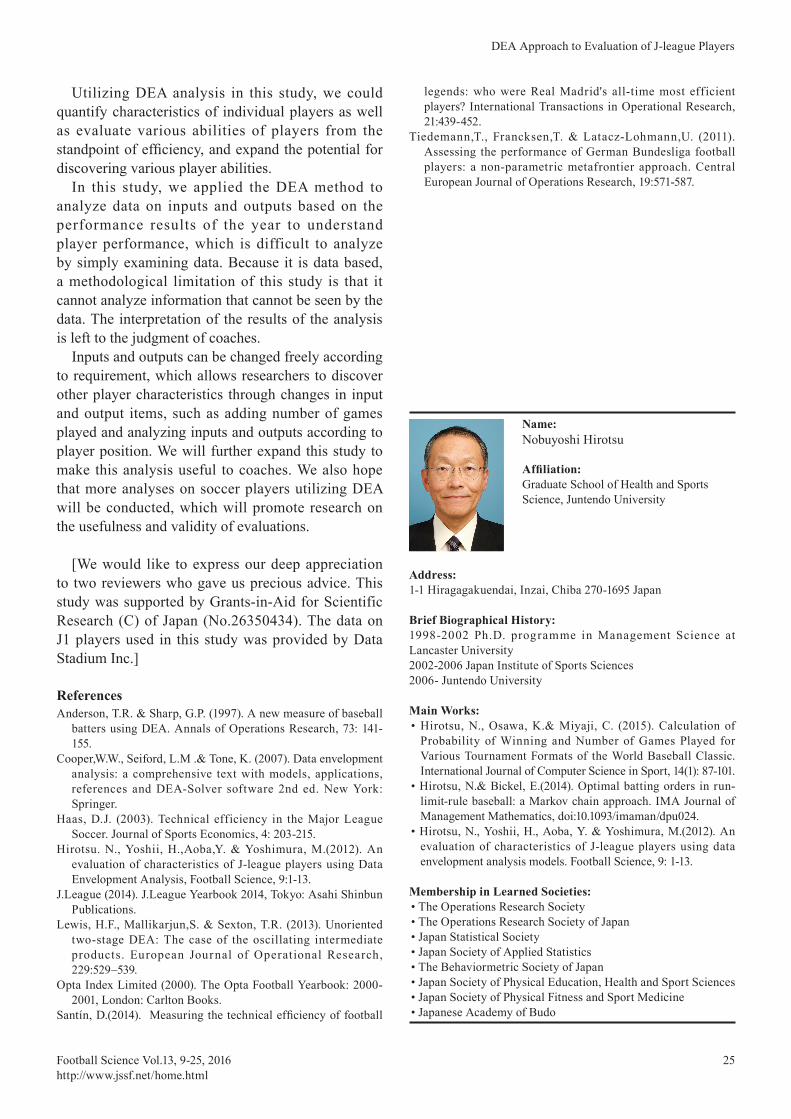
Name: Nobuyoshi Hirotsu

Affiliation: Graduate School of Health and Sports Science, Juntendo University

Address:1-1 Hiragagakuendai, Inzai, Chiba 270-1695 Japan

Brief Biographical History:1998-2002 Ph.D. programme in Management Science at Lancaster University2002-2006 Japan Institute of Sports Sciences2006- Juntendo University

Main Works:• Hirotsu, N., Osawa, K.& Miyaji, C. (2015). Calculation of

Probability of Winning and Number of Games Played for Various Tournament Formats of the World Baseball Classic. International Journal of Computer Science in Sport, 14(1): 87-101.

• Hirotsu, N.& Bickel, E.(2014). Optimal batting orders in run-limit-rule baseball: a Markov chain approach. IMA Journal of Management Mathematics, doi:10.1093/imaman/dpu024.

• Hirotsu, N., Yoshii, H., Aoba, Y. & Yoshimura, M.(2012). An evaluation of characteristics of J-league players using data envelopment analysis models. Football Science, 9: 1-13.

Membership in Learned Societies:• The Operations Research Society• The Operations Research Society of Japan• Japan Statistical Society• Japan Society of Applied Statistics• The Behaviormetric Society of Japan• Japan Society of Physical Education, Health and Sport Sciences• Japan Society of Physical Fitness and Sport Medicine• Japanese Academy of Budo

Paper : Football (Soccer) A DEA Approach to Evaluating ... · DEA allows a relative evaluation...

Documents

Transcript of Paper : Football (Soccer) A DEA Approach to Evaluating ... · DEA allows a relative evaluation...