Paper de Referencia
28
University of Connecticut DigitalCommons@UConn Economics Working Papers Department of Economics 1-1-2005 Determinan ts of Poverty in Kenya: A Household Level Analysis Alemayehu Geda Institute of Soc ial Studies, Te H ague and Addis Aba ba University Niek de Jong Institute of Soc ial Studies, Te H ague Mwangi S. Kimenyi University of Connecticut Germano Mwabu University of Nairobi and Yale University Follow this and additional works at: hp://digitalcommons.uconn.edu/econ_wpapers Part of the Economics Commons Tis Article is brought to you for free and open access by the Department of Economics at DigitalCommons@UConn. I t has been accepted for inclusion in Economics Working Papers by an authorized administrator of DigitalCommons@UC onn. For more information, please contact [email protected] . Recommended Citation Geda, Alemayehu; de Jong, Niek; Kimenyi, Mwangi S.; and Mwabu, Germano, "Determinants of Poverty in Kenya: A Household Level Analysis" (2005). Economics W orking P apers. Paper 200544. hp://digitalcommons.uconn.edu/econ_wpapers/200544
-
Upload
richterdavidrojasdelgado -
Category
Documents
-
view
215 -
download
0
Transcript of Paper de Referencia
8/18/2019 Paper de Referencia
http://slidepdf.com/reader/full/paper-de-referencia 1/28
University of Connecticut
DigitalCommons@UConn
Economics Working Papers Department of Economics
1-1-2005
Determinants of Poverty in Kenya: A HouseholdLevel Analysis
Alemayehu Geda Institute of Social Studies, Te Hague and Addis Ababa University
Niek de Jong Institute of Social Studies, Te Hague
Mwangi S. KimenyiUniversity of Connecticut
Germano MwabuUniversity of Nairobi and Yale University
Follow this and additional works at: hp://digitalcommons.uconn.edu/econ_wpapers
Part of the Economics Commons
Tis Article is brought to you for free and open access by the Department of Economics at DigitalCommons@UConn. It has been accepted for
inclusion in Economics Working Papers by an authorized administrator of DigitalCommons@UConn. For more information, please contact
Recommended CitationGeda, Alemayehu; de Jong, Niek; Kimenyi, Mwangi S.; and Mwabu, Germano, "Determinants of Poverty in Kenya: A HouseholdLevel Analysis" (2005). Economics Working Papers. Paper 200544.hp://digitalcommons.uconn.edu/econ_wpapers/200544
8/18/2019 Paper de Referencia
http://slidepdf.com/reader/full/paper-de-referencia 2/28
Department of Economics Working Paper Series
Determinants of Poverty in Kenya: A Household Level Analysis
Alemayehu GedaInstitute of Social Studies and Addis Ababa University
Niek de JongInstitute of Social Studies, The Hague
Mwangi S. KimenyiUniversity of Connecticut
Germano MwabuUniversity of Nairobi and Yale University
Working Paper 2005-44
January 2005
341 Mansfield Road, Unit 1063
Storrs, CT 06269–1063
Phone: (860) 486–3022
Fax: (860) 486–4463http://www.econ.uconn.edu/
This working paper is indexed on RePEc, http://repec.org/
8/18/2019 Paper de Referencia
http://slidepdf.com/reader/full/paper-de-referencia 3/28
Abstract
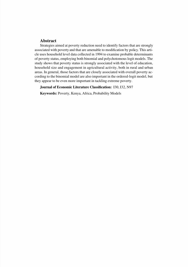
Strategies aimed at poverty reduction need to identify factors that are stronglyassociated with poverty and that are amenable to modification by policy. This arti-
cle uses household level data collected in 1994 to examine probable determinants
of poverty status, employing both binomial and polychotomous logit models. The
study shows that poverty status is strongly associated with the level of education,
household size and engagement in agricultural activity, both in rural and urban
areas. In general, those factors that are closely associated with overall poverty ac-
cording to the binomial model are also important in the ordered-logit model, but
they appear to be even more important in tackling extreme poverty.
Journal of Economic Literature Classification: I30, I32, N97
Keywords: Poverty, Kenya, Africa, Probability Models
8/18/2019 Paper de Referencia
http://slidepdf.com/reader/full/paper-de-referencia 4/28
1
I. INTRODUCTION1
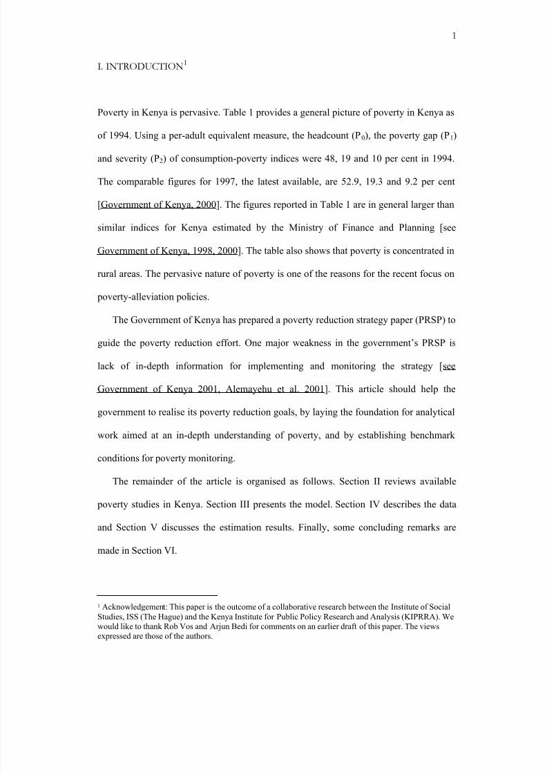
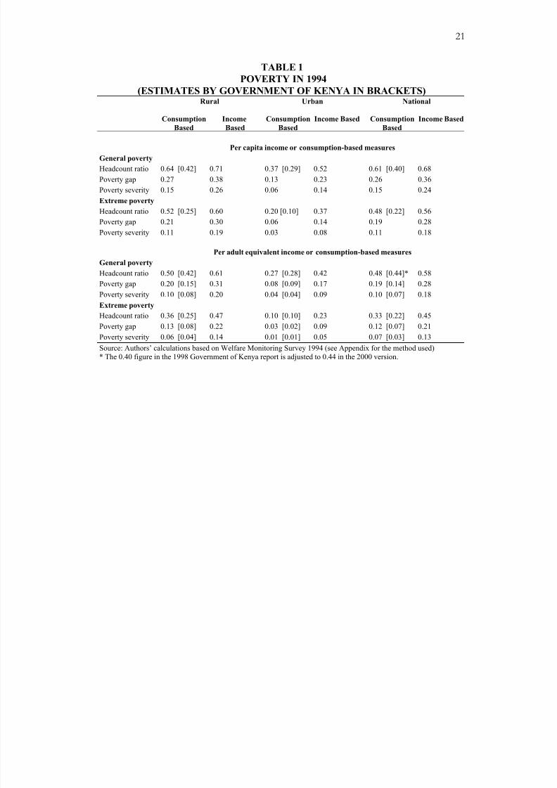
Poverty in Kenya is pervasive. Table 1 provides a general picture of poverty in Kenya as
of 1994. Using a per-adult equivalent measure, the headcount (P0), the poverty gap (P1)
and severity (P2) of consumption-poverty indices were 48, 19 and 10 per cent in 1994.
The comparable figures for 1997, the latest available, are 52.9, 19.3 and 9.2 per cent
[Government of Kenya, 2000]. The figures reported in Table 1 are in general larger than
similar indices for Kenya estimated by the Ministry of Finance and Planning [see
Government of Kenya, 1998, 2000]. The table also shows that poverty is concentrated in
rural areas. The pervasive nature of poverty is one of the reasons for the recent focus on
poverty-alleviation policies.
The Government of Kenya has prepared a poverty reduction strategy paper (PRSP) to
guide the poverty reduction effort. One major weakness in the government’s PRSP is
lack of in-depth information for implementing and monitoring the strategy [see
Government of Kenya 2001, Alemayehu et al. 2001]. This article should help the
government to realise its poverty reduction goals, by laying the foundation for analytical
work aimed at an in-depth understanding of poverty, and by establishing benchmark
conditions for poverty monitoring.
The remainder of the article is organised as follows. Section II reviews available
poverty studies in Kenya. Section III presents the model. Section IV describes the data
and Section V discusses the estimation results. Finally, some concluding remarks are
made in Section VI.
1 Acknowledgement: This paper is the outcome of a collaborative research between the Institute of Social
Studies, ISS (The Hague) and the Kenya Institute for Public Policy Research and Analysis (KIPRRA). We
would like to thank Rob Vos and Arjun Bedi for comments on an earlier draft of this paper. The views
expressed are those of the authors.
8/18/2019 Paper de Referencia
http://slidepdf.com/reader/full/paper-de-referencia 5/28
2
II. PREVIOUS POVERTY STUDIES IN KENYA
Analytical work on determinants of poverty in Kenya is at best scanty. Most of the
available studies are descriptive and focus mainly on measurement issues. Earlier
poverty studies have focused on a discussion of inequality and welfare based on limited
household level data [see Bigsten 1981, Hazlewood 1981, House and Killick 1981]. One
recent comprehensive study on the subject is that of Mwabu et al. [2000], which deals
with measurement, profile and determinants of poverty. The study employs a household
welfare function, approximated by household expenditure per adult equivalent. The
authors run two categories of regressions, using overall expenditures and food
expenditures as dependent variables. In each of the two cases, three equations are
estimated which differ by type of dependent variable. These dependent variables are:
total household expenditure, total household expenditure gap (the difference between the
absolute poverty line and the actual expenditure) and the square of the latter. A similar
set of dependent variables is used for food expenditure, with the explanatory variables
being identical in all cases.
Mwabu et al. [2000] justified their choice of this approach (compared to a
logit/probit model) as follows. First, the two approaches (discrete and continuous choice-
based regressions) yield basically similar results (see below, however); second, the
logit/probit model involves unnecessary loss of information in transforming household
expenditure into binary variables. Although their specification is simple and easy to
follow, it has certain inherent weaknesses. One obvious weakness is that, unlike the
logit/probit model, the levels regression does not directly yield a probabilistic statement
8/18/2019 Paper de Referencia
http://slidepdf.com/reader/full/paper-de-referencia 6/28
3
about poverty. Second, the major assumption of the welfare function approach is that
consumption expenditures are negatively associated with absolute poverty at all
expenditure levels. Thus, factors that increase consumption expenditure reduce poverty.
However, this basic assumption needs to be taken cautiously. For instance, though
increasing welfare, raising the level of consumption expenditure of households that are
already above the poverty line does not affect the poverty level (as for example measured
by the headcount ratio).
Notwithstanding such weaknesses, the approach is widely used and the Mwabu et al.
[2000] study identified the following as important determinants of poverty: unobserved
region-specific factors, mean age, size of household, place of residence (rural versus
urban), level of schooling, livestock holding and sanitary conditions. The importance of
these variables does not change whether the total expenditure, the expenditure gap or the
square of the gap is taken as the dependent variable. The only noticeable change is that
the sizes of the estimated coefficients are enormously reduced in the expenditure gap and
in the square of the expenditure gap specifications. Moreover, except for minor changes
in the relative importance of some of the variables, the pattern of coefficients again
fundamentally remains unchanged when the regressions are run with food expenditure as
dependent variable.
Another recent study on the determinants of poverty in Kenya is Oyugi [2000],
which is an extension to earlier work by Greer and Thorbecke [1986a,b]. The latter study
used household calorie consumption as the dependent variable and a limited number of
household characteristics as explanatory variables. Oyugi [2000] uses both discrete and
continuous indicators of poverty as dependent variables and employs a much larger set of
household characteristics as explanatory variables. An important aspect of Oyugi’s study
8/18/2019 Paper de Referencia
http://slidepdf.com/reader/full/paper-de-referencia 7/28
4
is that it analyses poverty both at micro (household) and meso (district) level, with the
meso level analysis being the innovative component of the study.
Oyugi [2000] estimates a probit model using data of the 1994 Welfare Monitoring
Survey data. The explanatory variables (household characteristics) include: holding area,
livestock unit, the proportion of household members able to read and write, household
size, sector of economic activity (agriculture, manufacturing/industrial sector or
wholesale/retail trade), source of water for household use, and off-farm employment. The
results of the probit analysis show that almost all variables used are important
determinants of poverty in rural areas and at the national level, but that there are
important exceptions for urban areas [Oyugi, 2000]. These results are consistent with
those obtained from the meso-level regression analysis.
It is interesting to compare the implications of the levels [Mwabu et al. 2000] and
probit [Oyugi, 2000] regression approaches. From the levels regressions, age, household
size, residence, reading and writing and level of schooling are the top five important
determinants of poverty at the national level. In the probit model, however, in order of
importance the key determinants of poverty are: being able to read and write,
employment in off-farm activities, being engaged in agriculture, having a side-business
in the service sector, source of water and household size. Region of residence appears to
be equally important in determining poverty status in the two approaches. Although the
two approaches did not employ the same explanatory variables, this comparison points to
the possibility of arriving at different policy conclusions from the two approaches.
III. BINOMIAL AND POLYCHOTOMOUS MODELS OF POVERTY ANALYSIS
8/18/2019 Paper de Referencia
http://slidepdf.com/reader/full/paper-de-referencia 8/28
5
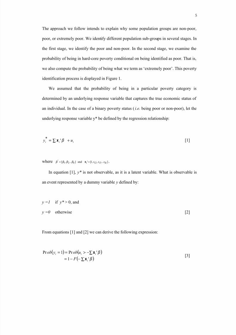
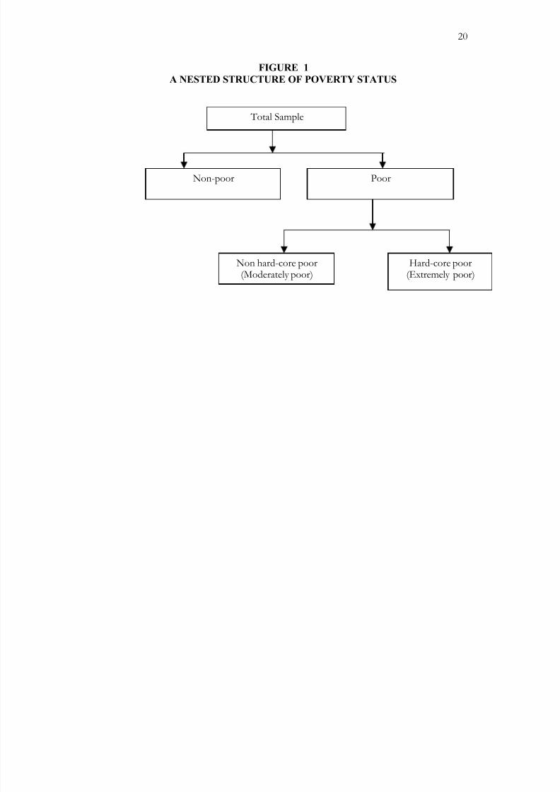
The approach we follow intends to explain why some population groups are non-poor,
poor, or extremely poor. We identify different population sub-groups in several stages. In
the first stage, we identify the poor and non-poor. In the second stage, we examine the
probability of being in hard-core poverty conditional on being identified as poor. That is,
we also compute the probability of being what we term as ‘extremely poor’. This poverty
identification process is displayed in Figure 1.
We assumed that the probability of being in a particular poverty category is
determined by an underlying response variable that captures the true economic status of
an individual. In the case of a binary poverty status ( i.e. being poor or non-poor), let the
underlying response variable y* be defined by the regression relationship:
∑ += iii u y '* β x [1]
where ]...,,1[' and ]...,[ 3221'
ik iiik x x x== xβ β β β .
In equation [1], y* is not observable, as it is a latent variable. What is observable is
an event represented by a dummy variable y defined by:
y =1 if y* > 0, and
y =0 otherwise [2]
From equations [1] and [2] we can derive the following expression:
( ) ( )
( )∑−−=
∑−>==
β
β
'1
'Pr 1Pr
i
iii
F
uob yob
x
x [3]
8/18/2019 Paper de Referencia
http://slidepdf.com/reader/full/paper-de-referencia 9/28
6
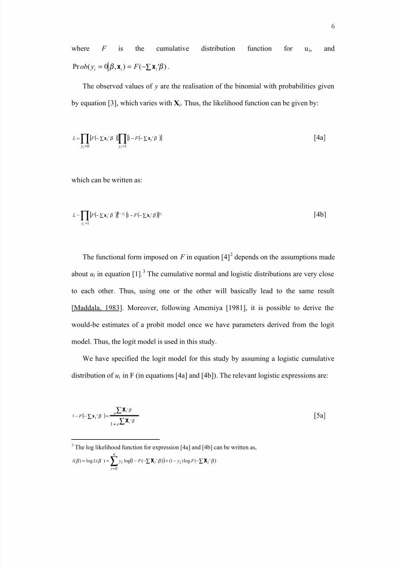
where F is the cumulative distribution function for ui, and
)'(),0(Pr β β ∑−== iii F yob xx .
The observed values of y are the realisation of the binomial with probabilities given
by equation [3], which varies with Xi. Thus, the likelihood function can be given by:
( )[ ] ( )[ ]∏ ∏= =
∑−−∑−=
0 1
'1'
i i y y
ii F F L β β xx [4a]
which can be written as:
( )[ ] ( )[ ]∏=
−∑−−∑−=
1
1 '1'
i
ii
y
yi
yi F F L β β xx [4b]
The functional form imposed on F in equation [4]2 depends on the assumptions made
about ui in equation [1].3 The cumulative normal and logistic distributions are very close
to each other. Thus, using one or the other will basically lead to the same result
[Maddala, 1983]. Moreover, following Amemiya [1981], it is possible to derive the
would-be estimates of a probit model once we have parameters derived from the logit
model. Thus, the logit model is used in this study.
We have specified the logit model for this study by assuming a logistic cumulative
distribution of ui in F (in equations [4a] and [4b]). The relevant logistic expressions are:
( )∑
∑
+
=−− ∑'
'
1
'1β
β
β i
i
e
e F i
x
xx [5a]
2 The log likelihood function for expression [4a] and [4b] can be written as,
( ) ∑∑ −−+−−== ∑=
)) '(log)1('(1log)(log)(
0
β β β β iii
n
i
i F y F y Ll xx
8/18/2019 Paper de Referencia
http://slidepdf.com/reader/full/paper-de-referencia 10/28
7
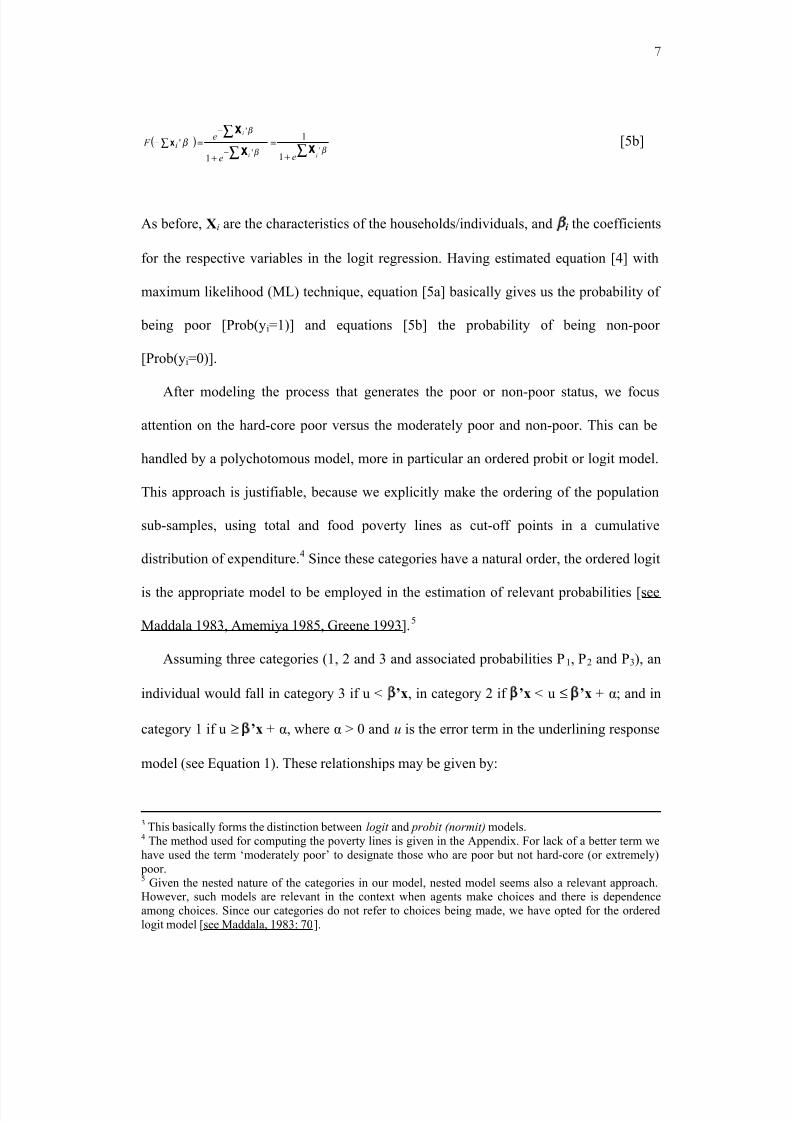
( )β β
β
β ''
'
1
1
1
'
ii
i
ee
e F i
∑∑
∑
+
=
+
=−−
−
∑xx
xx [5b]
As before, Xi are the characteristics of the households/individuals, and i the coefficients
for the respective variables in the logit regression. Having estimated equation [4] with
maximum likelihood (ML) technique, equation [5a] basically gives us the probability of
being poor [Prob(yi=1)] and equations [5b] the probability of being non-poor
[Prob(yi=0)].
After modeling the process that generates the poor or non-poor status, we focus
attention on the hard-core poor versus the moderately poor and non-poor. This can be
handled by a polychotomous model, more in particular an ordered probit or logit model.
This approach is justifiable, because we explicitly make the ordering of the population
sub-samples, using total and food poverty lines as cut-off points in a cumulative
distribution of expenditure.4 Since these categories have a natural order, the ordered logit
is the appropriate model to be employed in the estimation of relevant probabilities [see
Maddala 1983, Amemiya 1985, Greene 1993].5
Assuming three categories (1, 2 and 3 and associated probabilities P1, P2 and P3), an
individual would fall in category 3 if u < ’x, in category 2 if ’x < u ≤ ’x + α; and in
category 1 if u ≥ ’x + α, where α > 0 and u is the error term in the underlining response
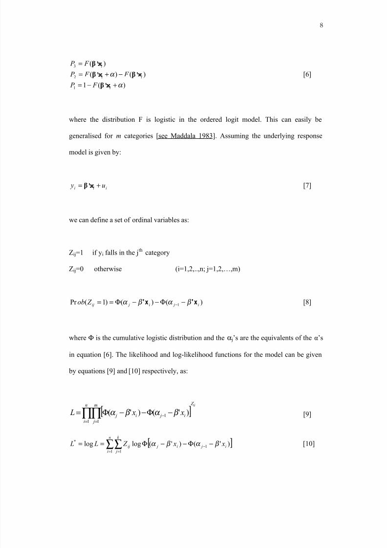
model (see Equation 1). These relationships may be given by:
3 This basically forms the distinction between logit and probit (normit) models.4 The method used for computing the poverty lines is given in the Appendix. For lack of a better term we
have used the term ‘moderately poor’ to designate those who are poor but not hard-core (or extremely)
poor.5 Given the nested nature of the categories in our model, nested model seems also a relevant approach.
However, such models are relevant in the context when agents make choices and there is dependence
among choices. Since our categories do not refer to choices being made, we have opted for the ordered
logit model [see Maddala, 1983: 70].
8/18/2019 Paper de Referencia
http://slidepdf.com/reader/full/paper-de-referencia 11/28
8
)(1
)()(
)(
1
2
3
α
α
+−=
−+=
=
i
ii
i
F P
F F P
F P
x'
x'x'
x'
β
ββ
β
[6]
where the distribution F is logistic in the ordered logit model. This can easily be
generalised for m categories [see Maddala 1983]. Assuming the underlying response
model is given by:
iii u y += x'β [7]
we can define a set of ordinal variables as:
Zij=1 if yi falls in the jth
category
Zij=0 otherwise (i=1,2,..,n; j=1,2,…,m)
)()()1(Pr 1 i ji jij Z ob x'x' β α β α −Φ−−Φ== − [8]
where Φ is the cumulative logistic distribution and the α j’s are the equivalents of the α’s
in equation [6]. The likelihood and log-likelihood functions for the model can be given
by equations [9] and [10] respectively, as:
[ ]ij Z n
i
m
j
i ji j x x L ∏∏= =
− −Φ−−Φ=1 1
1 )'()'( β α β α [9]
[ ])'()'(loglog 1
1 1
*
i ji j
n
i
k
j
ij x x Z L L β α β α −Φ−−Φ== −
= =
∑∑ [10]
8/18/2019 Paper de Referencia
http://slidepdf.com/reader/full/paper-de-referencia 12/28
9
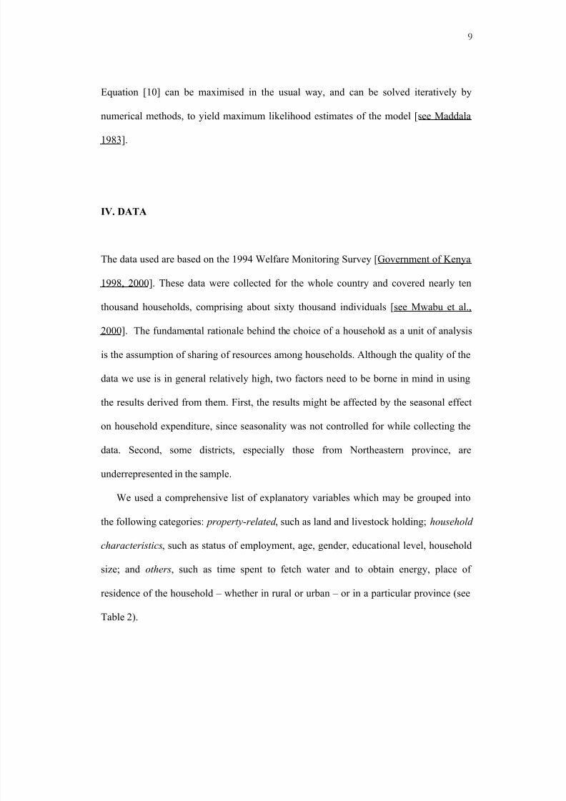
Equation [10] can be maximised in the usual way, and can be solved iteratively by
numerical methods, to yield maximum likelihood estimates of the model [see Maddala
1983].
IV. DATA
The data used are based on the 1994 Welfare Monitoring Survey [Government of Kenya
1998, 2000]. These data were collected for the whole country and covered nearly ten
thousand households, comprising about sixty thousand individuals [see Mwabu et al.,
2000]. The fundamental rationale behind the choice of a household as a unit of analysis
is the assumption of sharing of resources among households. Although the quality of the
data we use is in general relatively high, two factors need to be borne in mind in using
the results derived from them. First, the results might be affected by the seasonal effect
on household expenditure, since seasonality was not controlled for while collecting the
data. Second, some districts, especially those from Northeastern province, are
underrepresented in the sample.
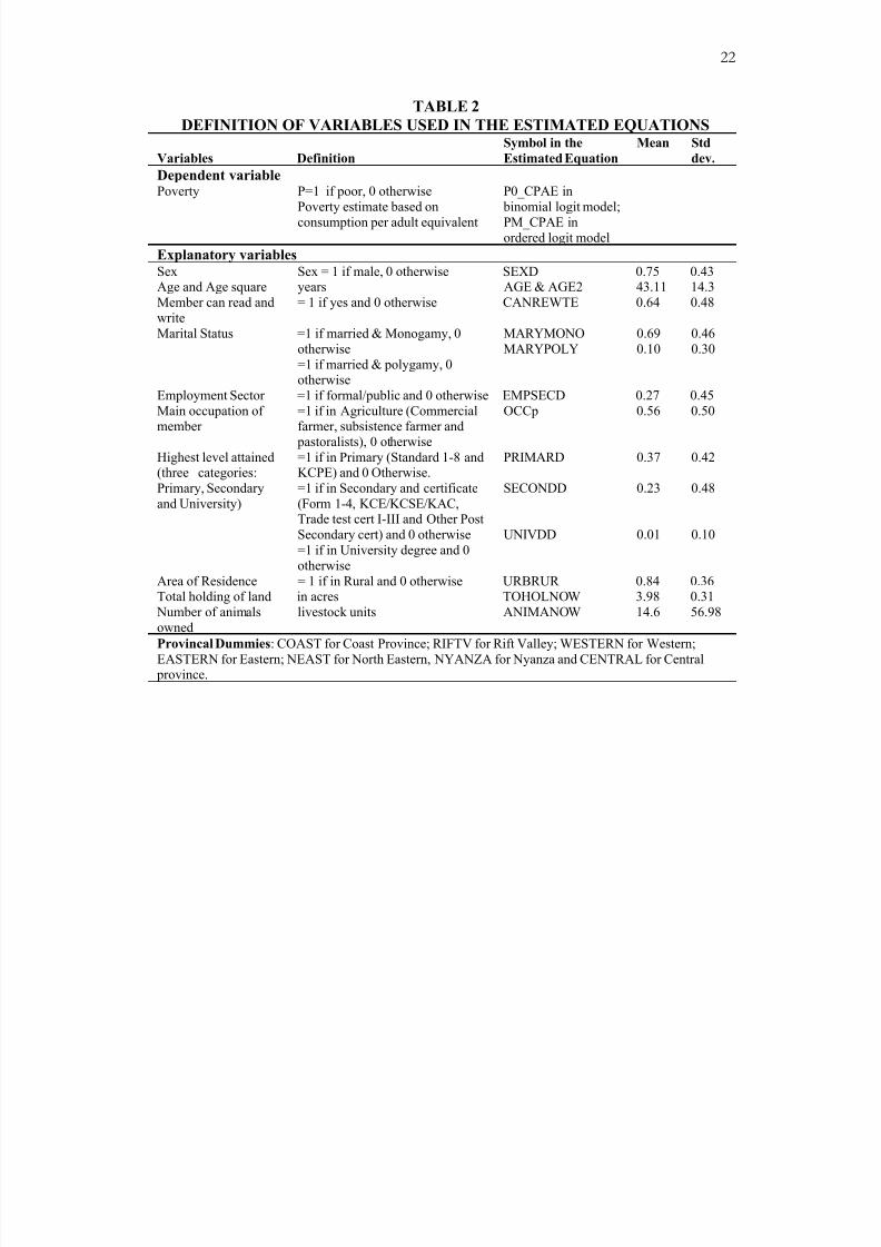
We used a comprehensive list of explanatory variables which may be grouped into
the following categories: property-related , such as land and livestock holding; household
characteristics, such as status of employment, age, gender, educational level, household
size; and others, such as time spent to fetch water and to obtain energy, place of
residence of the household – whether in rural or urban – or in a particular province (see
Table 2).
8/18/2019 Paper de Referencia
http://slidepdf.com/reader/full/paper-de-referencia 13/28
10
The estimation was made after inflating the number of households in the sample
(about 10,000) to that in the total population (nearly 26 million in 1994), using expansion
factors. The expansion factors are however adjusted downwards for children in case of
adult equivalent-based estimations. The household characteristics are assumed to affect
(adult-equivalent) members of the household equally.6
V. ESTIMATION RESULTS
Poverty Status: National Sample
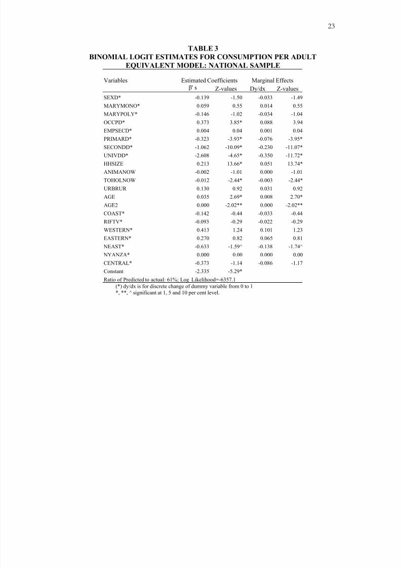
According to the estimation results, male-headed households are less likely to be poor.
Similarly, the likelihood of being poor is smaller in urban areas than in rural areas.
Probably to some extent related to this, people living in households mainly engaged in
agricultural activities are more likely to be poor, compared to households in
manufacturing activities. In all models the most important determinant of poverty status
is the level of education. The effects of this variable are similar across the four models.
The coefficient for household size is almost twice as high in the consumption-based as
income-based models ones, while the impacts of the sector of employment, as well as the
number of animals owned is insignificant in the consumption-based models. Total
holding of land does not seem to be important in any of the specifications. An
explanation for this may lie on the importance of the quality of land and/or lack of
complementary agricultural inputs [see Alemayehu et al. 2001]. Table 3 shows the
estimated model and the marginal effects of each explanatory variable on the probability
of being poor, based on models in which per adult equivalent consumption is used to
6 To save space, we have reported only those results derived from estimates based on poverty defined on
the basis of consumption per adult-equivalent. The interested reader is referred to Alemayehu et al. (2001)
for per capita and income-based estimates and related details.
8/18/2019 Paper de Referencia
http://slidepdf.com/reader/full/paper-de-referencia 14/28
11
estimate poverty. Estimation results using per capita income and consumption are
reported in Alemayehu et al. [2001].
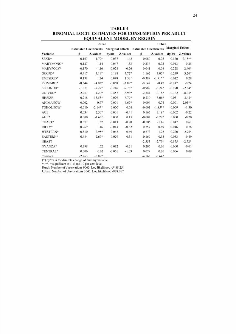
Poverty Status: Rural and Urban Sub-Samples
Following the finding that place of residence is associated with level of poverty, we have
fitted the model to data for rural and urban areas separately. The estimation results and
the marginal effects are given in Table 4. Again the detailed results are given in
Alemayehu et al. [2001]. In general, the results show that the factors strongly associated
with poverty (level of education, household size, engagement in agricultural activities)
are the same in both rural and urban areas. However, the size of the coefficients
associated with these regressors is larger in rural areas. Moreover, polygamous marriage
seems to worsen poverty in urban as opposed to rural areas. This may point at the larger
importance of labour input in rural rather than in urban economic activities. In rural areas
all the members of the extended household do often work in agriculture, while in urban
areas there may be less scope for all the members of the extended household to be
meaningfully engaged. This result does not seem to hold in the consumption-based
estimation, however . Given the reliability problem with income data and the fact that
even the consumption based estimates are not statistically significant at conventional
levels, this result may be taken as inconclusive. The consumption-based estimation yield
fairly similar results about determinants of poverty, particularly with regard to
educational attainment. The coefficients obtained in the latter model are relatively
smaller, however. Moreover, factors such as age, size of land holding (albeit with very
small coefficients) are found to be statistically significant in this version of the model.
Regional dummies for Western and Eastern provinces that are virtually insignificant in
the income-based model are found to be statistically significant in the consumption-
8/18/2019 Paper de Referencia
http://slidepdf.com/reader/full/paper-de-referencia 15/28
12
based version of the model for rural areas. Moreover, working in the urban modern
sector seems to reduce the likelihood of being poor.
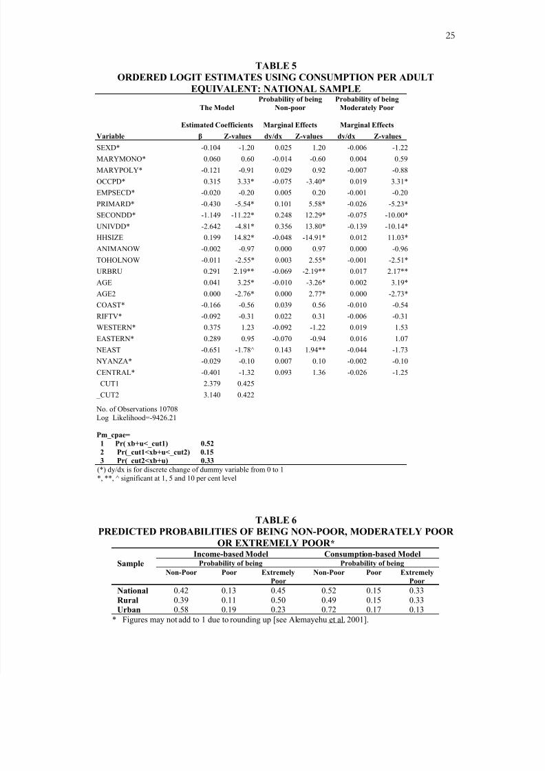
Ordered Poverty Status: National and Urban-Rural Sub-Samples
Following the discussion in Section 3, we have ordered the sample into three mutually
exclusive categories: non-poor (category 1), moderately poor (category 2) and hard-core
or extremely poor (category 3), with households in category 3 being most affected by
poverty. This classification is based on the poverty and food poverty lines computed
from the 1994 Welfare Monitoring Survey (see Appendix).
The estimated model and the marginal effects of the regressors for the consumption-
based models are given in Table 5. We noted that the consumption-based model is fairly
different from the income-based model. It exhibits regressors with statistically significant
coefficients as well as weaker explanatory effects in the case of category 1 (non-poor)
and category 2 (poor), respectively [see Alemayehu et al. 2001 for details].7
In general, it is interesting to note that those factors that are important in the binomial
model are still important in the ordered-logit model. More importantly, by comparing the
marginal effects for categories 2 and 3, we note that these variables are much more
important in tackling hard-core poverty than moderate poverty.
The ordered logit model is estimated for rural and urban sub-samples too (not
reported here, but available on request). Basically the results are similar to those obtained
for the national sample. However, the following interesting differences are observed.
First, although secondary and university level education are important both in rural and
urban areas, primary education is found to be extremely important in rural areas. Second,
agriculture as main occupation is more closely associated with poverty in urban areas
8/18/2019 Paper de Referencia
http://slidepdf.com/reader/full/paper-de-referencia 16/28
13
than in rural areas. This indicates that agriculture being the main occupation is a factor
that more strongly differentiates between being poor or non-poor in urban areas. Third,
the negative impact of aging is stronger in urban than rural areas. This may reflect the
collapse of the extended family network in urban areas, which normally serves as a
traditional insurance scheme in Africa. Finally, urban poverty is worst in Western and
Northeastern provinces [see Alemayehu et al. 2001].
The ordered-logit estimation of income-based models shows that at the national level
the predicted probability of falling in the non-poor category and into moderately and
extremely poor categories are 42, 13 and 45 percent, respectively. The corresponding
figures for rural areas are similar, while for urban areas they are 58, 19 and 23 percent
respectively. This basically shows that for a poor Kenyan residing in rural areas the
probability of falling in extreme poverty is much greater than for his/her urban
counterpart. A similar pattern is observed when the ordered logit model is estimated
using consumption-based data. However, the probability for the first category in general
declines while that for the third category rises. This information is summarised in Table
6. The details are given in Alemayehu et al. [2001].
The ordered-logit model results show clearly that determinants of poverty have
different impacts across the poverty categories defined. For instance, if we take the most
important determinant of poverty status in Kenya, i.e. thelevel of education, Table 4
shows that the marginal effect of having a primary level of education are 0.10, -0.03 and
-0.07 for non-poor, moderately poor and hard-core poor categories, respectively. The
comparable marginal effect figure for secondary level education are 0.25, -0.08 and -
0.16; and for university level education 0.36, -0.14 and -0.22, respectively. This shows
7 The marginal coefficients for category 3 (hard-core poor) are not reported as they could be derived from
the sum of the three, which should add to zero. This is because the probabilities of falling in either one of
the three categories adds up to one.
8/18/2019 Paper de Referencia
http://slidepdf.com/reader/full/paper-de-referencia 17/28
14
that, in general, education is more important for the hard-core poor than for the
moderately poor. The relative difference is largest in the case of primary education.
VI. CONCLUDING REMARKS
In this article an attempt has been made to explore the determinants of poverty in Kenya.
We have employed both binomial and polychotomous logit models using the 1994
Welfare Monitoring Survey data. Although a number of specific policy conclusions
could be drawn from the estimation results, the following policy implications of the
study stand out:
First, as expected, we have found that poverty is concentrated in rural areas in
general, and in the agricultural sector in particular. Being employed in the agricultural
sector accounts for a good part of the probability of being poor. Thus, investing in the
agricultural sector to reduce poverty should be a matter of great priority. Moreover, the
finding that the size of land holding is not a determinant of poverty status may suggest
the importance in poverty reduction not only of improving the quality of land, but also of
providing complementary inputs that may enhance productivity.
Second, the educational attainment of the head of the household (in particular high
school and university education) is found to be the most important factor that is
associated with poverty. Lack of education is a factor that accounts for a higher
probability of being poor. Thus, promotion of education is central in addressing
8/18/2019 Paper de Referencia
http://slidepdf.com/reader/full/paper-de-referencia 18/28
15
problems of moderate and extreme poverty. Specifically, primary education is found to
be of paramount importance in reducing extreme poverty in, particularly, rural areas.
Third, and related to the second point above, the importance of female education in
poverty reduction should be noted. We have found that female-headed households are
more likely to be poor than households of which the head is a men and that female
education plays a key role in reducing poverty. Thus, promoting female education should
be an important element of poverty reduction policies. Because there is evidence that
female education and fertility are negatively correlated, such a policy could also have an
impact on household size, which is another important determinant of poverty in Kenya.
Moreover, given the importance of female labour in rural Kenya and elsewhere in Africa,
investing in female education should be productivity enhancing.
Finally, in line with the three strategies that are outlined in the PRSP and directly
related to issues of poverty (economic growth and macro stability, raising income
opportunity of the poor, and improving quality of life), the findings in this study point to
the importance of focusing on education in general and primary education in rural areas
in particular. The study also highlights the higher likelihood of being poor of those who
are engaged in the agricultural sector. Thus, the PRSP’s strategy of raising income
opportunities of the poor should focus on investing in agriculture. Since the
macroeconomic environment is important in determining the productivity of such
investment, macroeconomic and political stability are a pre-requisite for addressing
poverty.
8/18/2019 Paper de Referencia
http://slidepdf.com/reader/full/paper-de-referencia 19/28
16
REFERENCES
Alemayehu, Geda, N. de Jong, M. Kimenyi and G. Mwabu, 2001, ‘Determinants of
Poverty in Kenya: Household Level Analysis’, KIPPRA Discussion Paper , July.
Amemiya, Takeshi, 1981, ‘Qualitative Response Model: A Survey’, Journal of
Economic Literature, Vol. 19, No. 4.
Amemiya, Takeshi, 1985, Advanced Econometrics, Cambridge: Cambridge University
Press.
Bigsten, Arne, 1981, ‘Regional Inequality in Kenya’ in Tony Killick. Papers on the
Kenyan Economy: Performance, Problems and Policies. Nairobi: Heinemann
Educational Books Ltd.
Government of Kenya, 1998, First Report on Poverty in Kenya: Incidence and Depth of
Poverty, Volume I. Nairobi: Ministry of Finance and Planning.
Government of Kenya, 2000, Second Report on Poverty in Kenya: Incidence and Depth
of Poverty, Volume I. Nairobi: Ministry of Finance and Planning.
Government of Kenya, 2001, Poverty Reduction Strategy Paper (PRSP) for the Period
2000-2003. Nairobi: The Government Printer.
Hazlewood, Arthur, 1981, ‘Income Distribution and Poverty: An Unfashionable View’ in
Tony Killick. Papers on the Kenyan Economy: Performance, Problems and
Policies. Nairobi: Heinemann Educational Books Ltd.
House, William and Tony Killick, 1981, ‘Inequality and Poverty in Rural Economy and
the Influence of Some Aspects of Policy’ in Tony Killick. Papers on the Kenyan
Economy: Performance, Problems and Policies. Nairobi: Heinemann Educational
Books Ltd.
8/18/2019 Paper de Referencia
http://slidepdf.com/reader/full/paper-de-referencia 20/28
17
Maddala, G.S., 1983, Limited Dependent and Qualitative Variables in Econometrics.
Cambridge: Cambridge University Press.
Manda, Kulundu, Mwangi Kimenyi and Germano Mwabu, 2001, ‘A Review of Poverty
and Antipoverty Initiatives in Kenya’, KIPPRA Working Paper (Forthcoming).
Mukherjee, C., H. White and M. Wuyts, 1998, Econometrics and Data Analysis for
Developing Countries. London: Routledge.
Mwabu, Germano, Wafula Masai, Rachel Gesami, Jane Kirimi, Godfrey Ndeng’e,
Tabitha Kiriti, Francis Munene, Margaret Chemngich and Jane Mariara, 2000,
‘Poverty in Kenya: Profile and Determinants’, Nairobi: University of Nairobi and
Ministry of Finance and Planning.
Oyugi, Lineth Nyaboke, 2000, ‘The Determinants of Poverty in Kenya’ (Unpublished
MA Thesis, Department of Economics, University of Nairobi).
Greer, J. and E. Thorbecke, 1986a, ‘A Methodology for Measuring Food Poverty
Applied to Kenya’, Journal Development Economics, Vol. 24, No. 1.
Greer, J. and E. Thorbecke, 1986b, ‘Food Poverty Profile Applied to Kenyan
Smallholders’ Economic Development and Cultural Change, Vol. 35, No. 1.
8/18/2019 Paper de Referencia
http://slidepdf.com/reader/full/paper-de-referencia 21/28
18
APPENDIX
Computations of Poverty Lines and Indices
There are a number of studies on the condition of poverty in Kenya, the most important
of which being the series of reports published by the Ministry of Finance and Planning.
In this paper, we have attempted to follow the method of poverty line determination used
by the Ministry of Finance and Planning. This is aimed at allowing for comparison with
the results of those studies.
The first step we took is to value the monthly food consumption required to satisfy
the 2250 calories that defines the biological minimum required per adult per day. This
food poverty line is computed by the Ministry of Finance and Planning for 1994 to be
Kshs. 874.72 for urban areas and Kshs.702.99 for rural areas per adult per month.
If, for illustration purposes, we take the urban areas, the procedure we adopted is as
follows. First we ranked the households according to per adult-equivalent expenditure on
food and identified the household that approximately spent Kshs. 874.72 per adult
equivalent on food items. Then we computed non-food consumption per adult
equivalent, by taking the mean non-food consumption per adult equivalent of those
households in the neighbourhood of this particular household (i.e. households with food
per adult-equivalent food expenditure in a band of +10% and –20% of the food poverty
line). Adding this mean non-food consumption, Kshs. 452.24, to the Kshs. 874.72 gives
the poverty line per adult equivalent of Kshs. 1326.96 per adult per month.
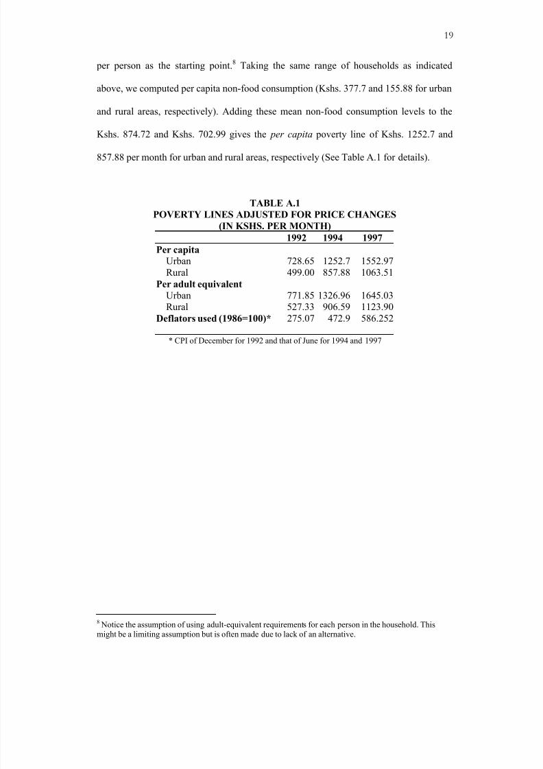
A similar procedure is followed to compute the per capita poverty line. We have used
the same Kshs. 874.72 for urban and Kshs. 702.99 for rural food requirement per month
8/18/2019 Paper de Referencia
http://slidepdf.com/reader/full/paper-de-referencia 22/28
19
per person as the starting point.8 Taking the same range of households as indicated
above, we computed per capita non-food consumption (Kshs. 377.7 and 155.88 for urban
and rural areas, respectively). Adding these mean non-food consumption levels to the
Kshs. 874.72 and Kshs. 702.99 gives the per capita poverty line of Kshs. 1252.7 and
857.88 per month for urban and rural areas, respectively (See Table A.1 for details).
TABLE A.1
POVERTY LINES ADJUSTED FOR PRICE CHANGES
(IN KSHS. PER MONTH)
1992 1994 1997
Per capita
Urban 728.65 1252.7 1552.97
Rural 499.00 857.88 1063.51Per adult equivalent
Urban 771.85 1326.96 1645.03
Rural 527.33 906.59 1123.90
Deflators used (1986=100)* 275.07 472.9 586.252
* CPI of December for 1992 and that of June for 1994 and 1997
8 Notice the assumption of using adult-equivalent requirements for each person in the household. This
might be a limiting assumption but is often made due to lack of an alternative.
8/18/2019 Paper de Referencia
http://slidepdf.com/reader/full/paper-de-referencia 23/28
20
FIGURE 1
A NESTED STRUCTURE OF POVERTY STATUS
Total Sample
Non-poor Poor
Hard-core poor
(Extremely poor)
Non hard-core poor
(Moderately poor)
8/18/2019 Paper de Referencia
http://slidepdf.com/reader/full/paper-de-referencia 24/28
21
TABLE 1
POVERTY IN 1994
(ESTIMATES BY GOVERNMENT OF KENYA IN BRACKETS)Rural Urban National
Consumption
Based
Income
Based
Consumption
Based
Income Based Consumption
Based
Income Based
Per capita income or consumption-based measures
General poverty
Headcount ratio 0.64 [0.42] 0.71 0.37 [0.29] 0.52 0.61 [0.40] 0.68
Poverty gap 0.27 0.38 0.13 0.23 0.26 0.36
Poverty severity 0.15 0.26 0.06 0.14 0.15 0.24
Extreme poverty
Headcount ratio 0.52 [0.25] 0.60 0.20 [0.10] 0.37 0.48 [0.22] 0.56
Poverty gap 0.21 0.30 0.06 0.14 0.19 0.28
Poverty severity 0.11 0.19 0.03 0.08 0.11 0.18
Per adult equivalent income or consumption-based measures
General poverty
Headcount ratio 0.50 [0.42] 0.61 0.27 [0.28] 0.42 0.48 [0.44]* 0.58Poverty gap 0.20 [0.15] 0.31 0.08 [0.09] 0.17 0.19 [0.14] 0.28
Poverty severity 0.10 [0.08] 0.20 0.04 [0.04] 0.09 0.10 [0.07] 0.18
Extreme poverty
Headcount ratio 0.36 [0.25] 0.47 0.10 [0.10] 0.23 0.33 [0.22] 0.45
Poverty gap 0.13 [0.08] 0.22 0.03 [0.02] 0.09 0.12 [0.07] 0.21
Poverty severity 0.06 [0.04] 0.14 0.01 [0.01] 0.05 0.07 [0.03] 0.13
Source: Authors’ calculations based on Welfare Monitoring Survey 1994 (see Appendix for the method used)* The 0.40 figure in the 1998 Government of Kenya report is adjusted to 0.44 in the 2000 version.
8/18/2019 Paper de Referencia
http://slidepdf.com/reader/full/paper-de-referencia 25/28
22
TABLE 2
DEFINITION OF VARIABLES USED IN THE ESTIMATED EQUATIONS
Variables Definition
Symbol in the
Estimated Equation
Mean Std
dev.
Dependent variablePoverty P=1 if poor, 0 otherwise
Poverty estimate based on
consumption per adult equivalent
P0_CPAE in
binomial logit model;
PM_CPAE inordered logit model
Explanatory variablesSex Sex = 1 if male, 0 otherwise SEXD 0.75 0.43Age and Age square years AGE & AGE2 43.11 14.3
Member can read and
write
= 1 if yes and 0 otherwise CANREWTE 0.64 0.48
Marital Status =1 if married & Monogamy, 0
otherwise
=1 if married & polygamy, 0otherwise
MARYMONO
MARYPOLY
0.69
0.10
0.46
0.30
Employment Sector =1 if formal/public and 0 otherwise EMPSECD 0.27 0.45
Main occupation ofmember
=1 if in Agriculture (Commercialfarmer, subsistence farmer and
pastoralists), 0 otherwise
OCCp 0.56 0.50
Highest level attained(three categories:
Primary, Secondary
and University)
=1 if in Primary (Standard 1-8 andKCPE) and 0 Otherwise.
=1 if in Secondary and certificate
(Form 1-4, KCE/KCSE/KAC,Trade test cert I-III and Other Post
Secondary cert) and 0 otherwise
=1 if in University degree and 0
otherwise
PRIMARD
SECONDD
UNIVDD
0.37
0.23
0.01
0.42
0.48
0.10
Area of Residence = 1 if in Rural and 0 otherwise URBRUR 0.84 0.36Total holding of land in acres TOHOLNOW 3.98 0.31
Number of animals
owned
livestock units ANIMANOW 14.6 56.98
Provincal Dummies: COAST for Coast Province; RIFTV for Rift Valley; WESTERN for Western;
EASTERN for Eastern; NEAST for North Eastern, NYANZA for Nyanza and CENTRAL for Central province.
8/18/2019 Paper de Referencia
http://slidepdf.com/reader/full/paper-de-referencia 26/28
23
TABLE 3
BINOMIAL LOGIT ESTIMATES FOR CONSUMPTION PER ADULT
EQUIVALENT MODEL: NATIONAL SAMPLE
Variables Estimated Coefficients Marginal Effectsβ' s Z-values Dy/dx Z-values
SEXD* -0.139 -1.50 -0.033 -1.49MARYMONO* 0.059 0.55 0.014 0.55
MARYPOLY* -0.146 -1.02 -0.034 -1.04
OCCPD* 0.373 3.85* 0.088 3.94
EMPSECD* 0.004 0.04 0.001 0.04
PRIMARD* -0.323 -3.93* -0.076 -3.95*
SECONDD* -1.062 -10.09* -0.230 -11.07*
UNIVDD* -2.608 -4.65* -0.350 -11.72*
HHSIZE 0.213 13.66* 0.051 13.74*
ANIMANOW -0.002 -1.01 0.000 -1.01
TOHOLNOW -0.012 -2.44* -0.003 -2.44*
URBRUR 0.130 0.92 0.031 0.92
AGE 0.035 2.69* 0.008 2.70*AGE2 0.000 -2.02** 0.000 -2.02**
COAST* -0.142 -0.44 -0.033 -0.44
RIFTV* -0.093 -0.29 -0.022 -0.29
WESTERN* 0.413 1.24 0.101 1.23
EASTERN* 0.270 0.82 0.065 0.81
NEAST* -0.633 -1.59^ -0.138 -1.74^
NYANZA* 0.000 0.00 0.000 0.00
CENTRAL* -0.373 -1.14 -0.086 -1.17
Constant -2.335 -5.29*
Ratio of Predicted to actual: 61%; Log Likelihood=-6357.1
(*) dy/dx is for discrete change of dummy variable from 0 to 1
*, **, ^ significant at 1, 5 and 10 per cent level.
8/18/2019 Paper de Referencia
http://slidepdf.com/reader/full/paper-de-referencia 27/28
24
TABLE 4
BINOMIAL LOGIT ESTIMATES FOR CONSUMPTION PER ADULT
EQUIVALENT MODEL BY REGION
Rural Urban
Estimated Coefficients Marginal Effects Estimated Coefficients Marginal Effects
Variable β Z-values dy/dx Z-values β Z-values dy/dx Z-values
SEXD* -0.163 -1.72^ -0.037 -1.42 -0.080 -0.25 -0.120 -2.18**
MARYMONO* 0.127 1.14 0.047 1.53 -0.236 -0.75 -0.013 -0.25
MARYPOLY* -0.170 -1.16 -0.028 -0.76 0.041 0.08 0.228 2.40*
OCCPD* 0.417 4.19* 0.198 7.72* 1.162 3.05* 0.249 3.20*
EMPSECD* 0.138 1.24 0.048 1.58^ -0.389 -1.91** 0.012 0.28
PRIMARD* -0.344 -4.02* -0.068 -3.08* -0.147 -0.47 -0.017 -0.24
SECONDD* -1.071 -9.27* -0.246 -9.78* -0.989 -3.24* -0.190 -2.84*
UNIVDD* -2.951 -4.20* -0.457 -8.93* -2.344 -3.18* -0.362 -8.03*
HHSIZE 0.218 13.55* 0.029 6.79* 0.230 5.06* 0.031 3.42*
ANIMANOW -0.002 -0.97 -0.001 -4.67* 0.004 0.74 -0.001 -2.05**
TOHOLNOW -0.010 -2.14** 0.000 0.08 -0.091 -1.85** -0.009 -1.30
AGE 0.034 2.50* -0.001 -0.41 0.165 3.18* -0.002 -0.22
AGE2 0.000 -1.63^ 0.000 0.15 -0.002 -3.29* 0.000 -0.20
COAST* 0.377 1.32 -0.013 -0.20 -0.385 -1.16 0.047 0.61
RIFTV* 0.269 1.16 -0.043 -0.82 0.257 0.69 0.046 0.76
WESTERN* 0.810 2.95* 0.042 0.69 0.673 1.25 0.220 2.76*
EASTERN* 0.684 2.67* 0.029 0.51 -0.169 -0.33 -0.033 -0.49
NEAST -2.553 -2.79* -0.175 -2.72*
NYANZA* 0.398 1.52 -0.012 -0.21 0.296 0.66 0.000 -0.01
CENTRAL* 0.006 0.02 -0.061 -1.09 0.079 0.20 0.006 0.09
Constant -2.763 -6.89* -4.563 -3.64*
(*) dy/dx is for discrete change of dummy variable*, **, ^ significant at 1, 5 and 10 per cent level Rural: Number of observations 9063, Log likelihood -5488.25
Urban: Number of observations 1645; Log likelihood -828.767
8/18/2019 Paper de Referencia
http://slidepdf.com/reader/full/paper-de-referencia 28/28
25
TABLE 5
ORDERED LOGIT ESTIMATES USING CONSUMPTION PER ADULT
EQUIVALENT: NATIONAL SAMPLE
The Model
Probability of being
Non-poor
Probability of being
Moderately Poor
Estimated Coefficients Marginal Effects Marginal Effects
Variable β Z-values dy/dx Z-values dy/dx Z-values
SEXD* -0.104 -1.20 0.025 1.20 -0.006 -1.22
MARYMONO* 0.060 0.60 -0.014 -0.60 0.004 0.59
MARYPOLY* -0.121 -0.91 0.029 0.92 -0.007 -0.88
OCCPD* 0.315 3.33* -0.075 -3.40* 0.019 3.31*
EMPSECD* -0.020 -0.20 0.005 0.20 -0.001 -0.20
PRIMARD* -0.430 -5.54* 0.101 5.58* -0.026 -5.23*
SECONDD* -1.149 -11.22* 0.248 12.29* -0.075 -10.00*
UNIVDD* -2.642 -4.81* 0.356 13.80* -0.139 -10.14*
HHSIZE 0.199 14.82* -0.048 -14.91* 0.012 11.03*
ANIMANOW -0.002 -0.97 0.000 0.97 0.000 -0.96
TOHOLNOW -0.011 -2.55* 0.003 2.55* -0.001 -2.51*
URBRU 0.291 2.19** -0.069 -2.19** 0.017 2.17**
AGE 0.041 3.25* -0.010 -3.26* 0.002 3.19*
AGE2 0.000 -2.76* 0.000 2.77* 0.000 -2.73*
COAST* -0.166 -0.56 0.039 0.56 -0.010 -0.54
RIFTV* -0.092 -0.31 0.022 0.31 -0.006 -0.31
WESTERN* 0.375 1.23 -0.092 -1.22 0.019 1.53
EASTERN* 0.289 0.95 -0.070 -0.94 0.016 1.07
NEAST -0.651 -1.78^ 0.143 1.94** -0.044 -1.73
NYANZA* -0.029 -0.10 0.007 0.10 -0.002 -0.10
CENTRAL* -0.401 -1.32 0.093 1.36 -0.026 -1.25
_CUT1 2.379 0.425
_CUT2 3.140 0.422
No. of Observations 10708
Log Likelihood=-9426.21
Pm_cpae=
1 Pr( xb+u<_cut1) 0.52
2 Pr(_cut1<xb+u<_cut2) 0.15
3 Pr(_cut2<xb+u) 0.33
(*) dy/dx is for discrete change of dummy variable from 0 to 1
*, **, ^ significant at 1, 5 and 10 per cent level
TABLE 6
PREDICTED PROBABILITIES OF BEING NON-POOR, MODERATELY POOR
OR EXTREMELY POOR *Income-based Model Consumption-based Model
Probability of being Probability of beingSampleNon-Poor Poor Extremely
Poor
Non-Poor Poor Extremely
Poor
National 0.42 0.13 0.45 0.52 0.15 0.33
Rural 0.39 0.11 0.50 0.49 0.15 0.33
Urban 0.58 0.19 0.23 0.72 0.17 0.13
* Figures may not add to 1 due to rounding up [see Alemayehu et al. 2001].