0

Panic on the Streets of London:

Police, Crime and the July 2005 Terror Attacks

Mirko Dracai, Stephen Machin

iiand Robert Witt

iii

July 2009 - Revised

Abstract

In this paper we study the causal impact of police on crime by looking at what happened

to crime and police before and after the terror attacks that hit central London in July

2005. The attacks resulted in a large redeployment of police officers to central London as

compared to outer London – in fact, police deployment in central London increased by

over 30 percent in the six weeks following the July 7 bombings, before sharply falling

back to pre-attack levels. During this time crime fell significantly in central relative to

outer London. Study of the timing of the crime reductions and their magnitude, the

subsequent sharp return back to pre-attack crime levels, the types of crime which were

more likely to be affected and a series of robustness tests looking at possible biases all

make us confident that our research approach identifies a causal impact of police on

crime. The instrumental variable approach we use uncovers an elasticity of crime with

respect to police of approximately -0.3, so that a 10 percent increase in police activity

reduces crime by around 3 percent.

Keywords: Crime; Police; Terror attacks.

JEL Classifications: H00, H5, K42.

Acknowledgements

We would like to thank Trevor Adams, Jay Gohil, Paul Leppard and Carol McDonald at

the Metropolitan Police and Gerry Weston at Transport for London for assistance with

the data used in this study. Helpful comments were received from three referees, the

Editor, Joshua Angrist, Christian Dustmann, Radha Iyengar, Alan Manning, Enrico

Moretti, from seminar participants at Aberdeen, Essex, LSE, UCL, the Paris School of

Economics and from participants in the 2007 Royal Economic Society annual conference

held in Warwick, the 2007 American Law and Economics Association annual meeting at

Harvard, the 2007 European Economic Association annual conference in Budapest and

the NBER Inter American Seminar in Economics in Buenos Aires. Amy Challen and

Richard Murphy contributed valuable research assistance. Any errors are our own. And,

of course, we must thank Morrissey and Marr for the title.

i Centre for Economic Performance, London School of Economics and Department of Economics,

University College London ii Department of Economics, University College London, Centre for the Economics of Education and

Centre for Economic Performance, London School of Economics iii

Department of Economics, University of Surrey

1

1. Introduction

Terrorism is arguably the single most significant topic of political discussion of

the past decade. In response, a small economic literature has begun to investigate the

causes and impacts of terrorism (see Krueger, 2006, for a summary or Krueger and

Maleckova, 2003, for some empirical work in this area). Terror attacks, or the threat

thereof, have also been considered in research on one important area of public policy,

namely the connections between crime and policing. Some recent studies (such as Di

Tella and Schargrodsky, 2004 and Klick and Taborrak, 2005) have used terrorism-

related events to look at the police-crime relationship since terror attacks can induce an

increased police presence in particular locations. This deployment of additional police

can, under certain conditions, be used to test whether or not increased police reduce

crime.

In this paper we also consider the crime-police relationship before and after a

terror attack, but in a very different context to other studies by looking at the increased

security presence following the terrorist bombs that hit central London in July 2005. Our

application is a more general one than the other studies in that it covers a large

metropolitan area following one of the most significant and widely known terror attacks

of recent years. The scale of the security response in London after these attacks provides

a good setting to examine the relationship between police and crime.

Moreover, and unlike the other studies in this area, we have very good data on

police deployment and can use these to identify the magnitude of the causal impact of

police on crime.1 Thus a major strength of this paper is that we are able to offer explicit

instrumental variable-based estimates of the police-crime elasticity which can be

compared to other estimates like Levitt’s (1997) contribution, that of Corman and Mocan

(2000) and Di Tella and Schrgrodsky’s (2004) implied elasticity. In fact, the sharp

discontinuity in police deployment that we able to identify using this data means we are

able to pin down this causal relation between crime and police very precisely. The

natural experiment that we consider also has some important external validity in the

sense that it involves the deployment of a clear “deterrence technology” (that is, more

police on the streets) rather than a simple measure of expenditures (e.g. as in Evans and

Owens, 2007, or Machin and Marie, 2009). Arguably, this type of visible increase in

1 Neither Di Tella and Schargrodsky (2004) nor Klick and Tabarrok (2005) had data on police activity.

2

police deployment is the main type of policy mechanism under discussion in public

debates about the funding and use of police resources.

Furthermore, the effectiveness of police is important in the context of a large

criminological literature that has generally failed to find significant impacts of police on

crime, even in quasi-experimental studies. Sherman and Weisburd (1995) review some

of the conclusions from this work. Gottfriedson and Hirschi (1990: 270) state that “no

evidence exists that augmentation of police forces or equipment, differential police

strategies, or differential intensities of surveillance have an effect on crime rates”.

Similar emphatic arguments are made by Felson(1994) and Klockars(1984).

The focus of the current paper is on what happened to criminal activity following

a large and unanticipated increase in police presence. The scale of the change in police

deployment that we study is much larger than in any of the other work in the crime-

police research field. Indeed, results reported below show that police activity in central

London increased by over 30 percent in the six weeks following the July 7 bombings as

part of a police deployment policy stylishly titled “Operation Theseus” by the authorities.

This police intervention represented the deployment of a very strong deterrence

technology. The coverage of police was more sustained, widespread and complete than

in any of the studies analysed in the existing literature. We therefore view the scale of

this change as important in addressing the paradox of the criminology literature

discussed above where it proves hard to detect crime reductions linked to increased

police presence. This is particularly the case since during the time period when police

presence was heightened, crime fell significantly in central London relative to outer

London. Both the timing of the crime reductions and the types of crime that were more

affected make us confident that this research approach identifies a causal impact of

police on crime. Moreover, when police deployments returned to their pre-attack levels

some six weeks later, the crime rate rapidly returned to its pre-attack level. Exploiting

these sharp discontinuities in police deployment we estimate an elasticity of crime with

respect to police of approximately -.3 to -.4, so that a 10 percent increase in police

activity reduces crime by around 3 to 4 percent. Furthermore, we are unable to find

evidence of either temporal or spatial displacement effects arising from the six-week

police intervention.

3

A crucial part of identifying a causal impact in this type of setting is establishing

the exclusion restriction which shows that terrorist attacks affect crime through the post-

attack increase in police deployment, rather than via other observable and unobservable

factors correlated with the attack or shock. This is important to generate credibility that

the findings inform the crime-police debate rather than being just about an episode where

a terror attack occurred. The police deployment data we use are invaluable here as (under

certain conditions) their availability make it possible to distinguish the impact of police

on crime from any general impact of the terrorist attack. In particular, our research

design features two interesting discontinuities related to the police intervention. The first

is the introduction of the geographically-focused police deployment policy in the week

of the terrorist attack. This immediate period surrounding the introduction of the policy

was also characterized by a series of correlated observable and unobservable shocks

related to the attack. In contrast, the second discontinuity associated with the withdrawal

of the policy occurred in a very different context. In this case, the observable and

unobservable shocks associated with the attack were still in effect and dissipating

gradually. Crucially though, the police deployment was discretely “switched off” after a

six week period and we observe an increase in crime that is exactly timed with this

change. Thus, we argue that is difficult to attribute this clear change in crime rates to

observable and unobservable shocks arising from the terrorist attacks. If these types of

shocks were significantly affecting crime rates then we would expect that effect to

continue even as the police deployment was being withdrawn. Indeed, an interesting

feature of our empirical results is just how clearly and definitively crime seems to

respond to a police presence.

The rest of the paper is organized as follows. Section 2 describes the events of

July 2005 and goes over the main modeling and identification issues. In Section 3 we

describe the data and provide an initial descriptive analysis. Section 4 presents the

statistical results and a range of additional empirical tests. Section 5 concludes.

2. Crime, Police and the London Terror Attacks

The Terror Attacks

In July 2005 London’s public transport system was subject to two waves of terror

attacks. The first occurred on Thursday 7th July and involved the detonation of four

4

bombs. The 32 boroughs of London are shown in Figure 1. Three of the bombs were

detonated on London Underground train carriages near the tube stations of Russell

Square (in the borough of Camden), Liverpool Street (Tower Hamlets) and Edgware

Road (Kensington and Chelsea). A fourth bomb was detonated on a bus in Tavistock

Square, Bloomsbury (Camden). The second wave of attacks occurred two weeks later on

the 21st July, consisting of four unsuccessful attempts at detonating bombs on trains near

the underground stations of Shepherds Bush (Kensington and Chelsea), the Oval

(Lambeth), Warren Street (Westminster) and on a bus in Bethnal Green (Tower

Hamlets). Despite the failure of the bombs to explode, this second wave of attacks

caused much turmoil in London. There was a large manhunt to find the four men who

escaped after the unsuccessful attacks and all of them were captured by 29th July.

Terror Attacks, Crime and Correlated Shocks

Di Tella and Schargrodsky (2004) were first to use police allocation policies in

the wake of terror attacks to circumvent the endogeneity problem of crime and police.

Using a July 1994 terrorist attack that targeted the main Jewish center in Buenos Aires,

they show that motor vehicle thefts fell significantly in areas where extra police were

subsequently deployed compared to areas several blocks away which did not receive

extra protection. Their effect is large (approximately a 75% reduction in thefts relative to

the comparison group) but also extremely local with no evidence that the police presence

reduced crime one or two blocks away from the protected areas. Another study by Klick

and Tabarrok (2005) uses terror alert levels in Washington DC to make inferences about

the police-crime relationship. The deployments they consider cover a more general area

but (as already discussed) are speculative since they are not able to quantify them with

data on police numbers or hours.

Both of these papers touch on the issue of correlated shocks to observables and

unobservables. However, in our case of London this could be a greater concern since the

terrorist attacks were a more significant, dislocating event for the city. Therefore, in

thinking about the question of correlated shocks, it is helpful to first consider a basic

equation in levels that describes the determinants of the crime rate in a set of

geographical areas (in our case, London boroughs) over time:

jt jt jt j t jk jtC = α + δP + λX + µ + τ + υ + ε (1)

5

where Cjt denotes the crime rate for borough j in period t, Pjt the level of police deployed

and Xjt is a vector of control variables that could be comprised of observable or

unobservable elements. The next set of terms are: jµ , a borough level fixed effect; tτ , a

common time effect (for example, to capture common weather or economic shocks); and

a final term jkυ which represents borough-specific seasonal effects with k indexing the

season (e.g. from 1-12 for monthly or 1-52 for a weekly frequency).2

Now consider a seasonally differenced version of equation (1), where the

dependent variable becomes the change in the area crime rate relative to the rate at the

same time in the previous year. This is highly important in crime modeling since crime is

strongly persistent across areas over time. In practical terms, this eliminates the

borough-level fixed effect and the borough-specific seasonality terms, yielding:

jt j(t-k) jt j(t-k) jt j(t-k) t t-k jt j(t-k)(C - C ) = α + δ(P -P ) + λ(X -X ) + (τ -τ ) + (ε - ε ) (2)

Note that the τt – τt-k difference term can now be interpreted as the year-on-year change

in factors that are common across all of the areas. By expressing this equation more

concisely we can make the correlated shocks issue explicit as follows:

k jt k jt k jt k t k jt∆ C = α + δ∆ P + λ∆ X + ∆ τ + ∆ ε (3)

where ∆ is a difference operator with k indexing the order of the seasonal differencing.

Using this framework we can carefully consider how a terrorist attack – which we

can denote generally as Z - affects the determinants of crime across areas. Following the

argument in the papers discussed above, the terror attack Z affects jtP∆ , shifting police

resources in a way that one can hypothesise is unrelated to crime levels. This hypothesis

is, of course, a crucial aspect of identification that needs serious consideration. For

example, it is possible that Z could affect the elements of jtX∆ creating additional

channels via which terrorist attacks could influence crime rates.

What are these potential impacts or channels? The economics of terrorism

literature stresses that the impacts of terrorism can be strong, but generally turn out to be

temporary (OECD, 2002; Bloom, 2009) in that economic activity tends to recover and

normalize itself fairly rapidly. Of course, a sharp but temporary shock would still have

2 These types of effects could prevail where seasonal patterns affect different boroughs with varying levels

of intensity. For example, the central London boroughs are more exposed to fluctuations due to tourism

activity and exhibit sharper seasonal patterns with respect to crime.

6

ample scope to intervene in our identification strategy by affecting crime in a way that is

correlated with the police response. In particular, three channels demand consideration.

First there is the physical dislocation caused by the attack. A number of tube stations

were closed and many Londoners changed their mode of transport after the attacks (e.g.

from the tube to buses or bicycles). This would have reshaped travel patterns and could

have affected the potential supply of victims for criminals in some areas. Secondly, the

volume of overall economic activity was affected. Studies on the aftermath of the attack

indicate that both international and domestic tourism fell after the attacks, as measured

by hotel vacancy rates, visitor spending data and counts of domestic day trips (Greater

London Authority, 2005). Finally, there may be a psychological impact on individuals in

terms of their attitudes towards risk. As Becker and Rubinstein (2004) outline, this

influences observable travel decisions as well as more subtle unobservable behavior.

To summarize, we think of these effects as being manifested in three elements of

the Xjt vector outlined above:

1 2

jt jt jt jtX = [X , X , θ ] (4)

In (4), 1

jtX is a set of exogenous control variables (observable to researchers), that is

observable factors such as area-level labour market conditions that change slowly and

are unlikely to be immediately affected by terrorist attacks (if at all). The second 2

jtX

vector represents the observable factors that change more quickly and are therefore

vulnerable to the dislocation caused by terrorist attacks. As discussed above, here we are

thinking primarily of factors such as travel patterns which could influence the potential

supply of victims to crime across areas. The final element jtθ then captures an analogous

set of unobservable factors that are susceptible to change due to the terrorist attack. In

the spirit of Becker and Rubinstein’s (2004) discussion, the main factor to consider here

is fear or how individuals handle the risks associated with terrorism. For example, it is

plausible that, in the wake of the attacks, commuters in London became more vigilant to

suspicious activity in the transport system and in public spaces. This vigilance would

have been focused mainly on potential terrorist activity, but one might expect that this

type of cautious behaviour could have a spillover onto crime.

The implications of these correlated shocks for our identification strategy can

now be clearly delineated. For our exclusion restriction to hold it needs to be shown that

7

the terrorist attack Z affected the police deployment in a way that can be separately

identified from Z’s effect on other observable and unobservable factors that can

influence crime rates. Practically, we show this later in the paper by mapping the timing

and location of the police deployment shock and comparing it to the profiles of the

competing observable and unobservable shocks.

Possible Displacement Effects

Another issue that could potentially affect our identification strategy is that of

crime displacement. Since the police intervention affected the costs of crime across

locations and time, it may be that criminals take these changes into account and adjust

their behavior. This raises the possibility that criminal activity was either diverted into

other areas (e.g. the comparison group of boroughs) during Operation Theseus or

postponed until after the extra police presence was withdrawn. The implication then is

that simple differences-in-differences estimates of the police effect on crime would be

upwardly biased if these offsetting spatial displacement effects are not taken into

account. Temporal displacement can have the opposite effect and we discuss this more

in the final empirical section.

3. Data Description and Initial Descriptive Analysis

Data

We use daily police reports of crime from the London Metropolitan Police

Service (LMPS) before and after the July 2005 terrorist attacks. Our crime data cover the

period from 1st January 2004 to 31st December 2005 and are aggregated up from ward

to borough level and from days to weeks over the two year period. There are 32 London

boroughs as shown on the map in Figure 1.3 There are also monthly borough level data

available over a longer time period that we use for some robustness checks.

The basic street-level policing of London is carried out by 33 Borough

Operational Command Units (BOCUs), which operate to the same boundaries as the 32

London borough councils apart from one BOCU which is dedicated to Heathrow Airport.

We have been able to put together a weekly panel covering 32 London boroughs over

two years giving 3,328 observations. Crime rates are calculated on the basis of

3 The City of London has its own police force and so this small area is excluded from our analysis.

8

population estimates at borough level, supplied by the Office of National Statistics

(ONS) online database.4

The police deployment data are at borough level and were produced under special

confidential data-sharing agreements with the LMPS. The main data source used is

CARM (Computer Aided Resource Management), the police service’s human resource

management system. This records hours worked by individual officers on a daily basis.

We aggregate the deployment data to borough-level since the CARM data is mainly

defined at this level. However, there is also useful information on the allocation of hours

worked by incident and/or police operation.5 While hours worked are available according

to officer rank our main hours measure is based on total hours worked by all officers in

the borough adjusted for this reallocation effect. In addition to crime and deployment, we

have also obtained weekly data on tube journeys for all stations from Transport for

London (TFL). It is daily borough-level data aggregated up to weeks based on entries

into and exits from tube stations. Finally, we also use data from the UK Labour Force

Survey (LFS) to provide information on local labour market conditions.

Initial Approach

Our analysis begins by looking at what happened to police deployment and crime

before and after the July 2005 terror attacks in London using a differences-in-differences

approach. This rests upon defining a treatment group of boroughs in central and inner

London where the extra police deployment occurred and comparing their crime

outcomes to the other, non-treated boroughs. The police hours data we use facilitates the

development of this approach, with two features standing out. First, the data allow us to

measure the increase in total hours worked in the period after the attacks. The increase in

total hours was accomplished through the increased use of overtime shifts across the

police service and this policy lasted approximately six weeks. Secondly, the police data

contain a special resource allocation code denoted as Central Aid. This code allows us to

identify how police hours worked were geographically reallocated over the six-week

period. For example, we can identify how hours worked by officers stationed in the outer

London boroughs were reallocated to public security duties in central and inner London.

4 Web Appendix Table A1 shows some summary statistics on the crime data.

5 Since the CARM information is also used for calculating police pay it is considered a very reliable

measure of police activity. We gained access to this data after repeated inquiries to the MPS. The main

condition for access was that we not reveal any strategic information about ongoing or individual,

borough-specific police deployment policies.

9

The extra hours were mainly reallocated to the boroughs of Westminster, Camden,

Islington, Kensington and Chelsea, and Tower Hamlets, with individual borough

allocations being proportional to the number of Tube stations in the borough.6 These

boroughs either contained the sites of the attacks or featured many potential terrorist

targets such as transport nodes or significant public spaces. Using these two features of

the data we are able to define a treatment group comprised of the five named boroughs.

A map showing the treatment group is given in Figure 1. In most of the descriptive

statistics and modeling below we use all other boroughs as the comparison group in

order to simplify the analysis.

What did the extra police deployment in the treated boroughs entail? The number

of mobile police patrols were greatly increased and officers were posted to guard major

public spaces and transport nodes, particularly tube stations. In areas of central London

where many stations were located this resulted in a highly visible police presence and

this is confirmed by public surveys conducted at the time.7 Given this high visibility we

think of it as potentially exerting a deterrent effect on public, street-level crimes such as

thefts and violent assault. We test for this prediction in the empirical work.

Basic Differences-in-Differences

In Table 1 we compare what happened to police deployment and to total crime

rates before and after the July 2005 terror attacks in the treatment group boroughs as

compared to all other boroughs. Police deployment is measured in a similar way to crime

rates, that is, we normalize police hours worked by the borough population. Following

the discussion in Section 2 we define the before and after periods in year-on-year,

seasonally adjusted terms. This ensures that we are comparing like-with-like in terms of

the seasonal effects prevailing at a given time of the year. For example, looking at Table

1 the crime rate of 4.03 per 1000 population in panel B represents the treatment group

crime rate in the period from the 8th

of July 2004 until the 19th

of August 2004. The post-

6 We say “mainly reallocated” due to the fact that some mobile patrols crossed into adjacent boroughs and

because some bordering areas of boroughs were the site of some small deployments. A good case here is

the southern tip of Hackney borough (between Islington and Tower Hamlets). However, the majority of

Hackney was not treated by the policy (since this borough is notoriously lacking in Tube station links) so

we exclude it from the treatment group. 7 Table A2 of the Web Appendix reports the results of a survey of London residents in the aftermath of the

attacks. Approximately 70 percent of respondents from inner London attested to a higher police presence

in the period since the attacks. The lower percentage reported by outer London residents also supports the

hypothesis of differential deployment across areas.

10

period or “policy on” period then runs from July 7th

2005 until August 18th

2005 with a

crime rate of 3.59.8 Thus by taking the difference between these “pre” and “post” crime

rates we are able to derive the year-on-year, seasonally adjusted change in crime rates

and police hours. These are then differenced across the treatment (T = 1) and comparison

(T = 0) groups to get the customary differences-in-differences (DiD) estimate.

The first panel of Table 1 shows unconditional DiD estimates for police hours. It

is clear that the treatment boroughs experienced a very large relative change in police

deployment. Per capita hours worked increased by 34.6% in the DiD (final row, column

3). Arguably, the composition of this relative change is almost as important for our

experiment as the scale. The relative change was driven by an increase in the treatment

group (of 72.8 hours per capita) with little change in hours worked for the comparison

group (only 2.2 hours more per capita). This was feasible because of the large number of

overtime shifts worked. In practice, it means that while there was a diversion of police

resources from the comparison boroughs to the treatment boroughs the former areas were

able to keep their levels of police hours constant. Obviously, this ceteris paribus feature

greatly simplifies our later analysis of displacement effects since we do not have to deal

with the implications of a zero-sum shift of resources across areas. The next panel of

Table 1 deals with the crime rates. It shows that crime rates fell by 11.1% in the DiD

(final row, column 6). Again, this change is driven by a fall in treatment group crime

rates and a steady crime rate in the comparison group. This is encouraging since it is

what would be expected from the type of shift we have just seen in police deployment.

A visual check of weekly police deployment and crime rates is offered in Figures

2a and 2b. Here we do two things. First, we normalize crime rates and police hours

across the treatment and comparison groups by their level in week one of our sample (i.e.

January 2004). This re-scales the levels in both groups so that we can directly compare

their evolution over time. Secondly, we mark out the attack or “policy-on” period in

2005 along with the comparison period in the previous year. As Figure 2a shows, this

reveals a clear, sharp discontinuity in police deployment. Police hours worked in the

treatment group rise immediately after the attack and fall sharply at the end of the six

week Operation Theseus period.

8 The one day difference in calendar date across years ensures we compare the same days of the week.

11

The visual evidence for the crime rate in Figure 2b is less decisive because the

weekly crime rates are clearly more volatile than the police hours data. This is to be

expected insofar as police hours are largely determined centrally by policy-makers, while

crime rates are essentially the outcomes of decentralized activity. This volatility does

raise the possibility that the fall in crime rates seen in the Table 1 DiD estimates may

simply be due to naturally occurring, short-run time series volatility rather than the result

of a policy intervention – a classic problem in the literature (Donohue, 1998). After the

correlated shocks issue this is probably the biggest modeling issue in the paper and we

deal with it extensively in the next section.

4. Statistical Models of Crime and Police

In this section we present our statistical estimates. We begin with a basic set of

estimates and then move on to focus on specific issues to do with different crime types,

timing, correlated shocks and displacement effects.

Statistical Approach

The starting point for the statistical work is a DiD model of crime determination.

We have borough level weekly data for the two calendar years 2004 and 2005. The terror

attack variable (Z as discussed above) is specified as an interaction term Tb*POSTt,

where T denotes the treatment boroughs and POST is a dummy variable equal to one in

the post-attack period.

In this setting the basic reduced form seasonally differenced weekly models for

police deployment and crime (with lower case letters denoting logs) are:

52 bt 1 1 t 1 b t 1 52 bt 52 1bt∆ p = α + β POST + δ (T *POST ) + λ ∆ x + ∆ ε (5)

52 bt 2 2 t 2 b t 2 52 bt 52 2bt∆ c = α + β POST + δ (T *POST ) + λ ∆ x + ∆ ε (6)

Because of the highly seasonal nature of crime noted above, the equations are

differenced across weeks of the year (hence the k = 52 subscript in the ∆k differences).

The key parameters of interest are the δ’s, which are the seasonally adjusted differences-

in-differences estimates of the impact of the terror attacks on police deployment and

crime.

These reduced form equations can be combined to form a structural model

relating crime to police deployment, from which we can identify the causal impact of

police on crime. The structural equation is:

12

52 bt 3 3 t 3 52 bt 3 52 bt 52 3bt∆ c = α + β POST + δ p + λ ∆ x + ∆ ε∆ (7)

where the variation in police deployment induced by the terror attacks identifies the

causal impact of police on crime. The first stage regression is equation (5) above and so

equation (7) is estimated by instrumental variables (IV) where the Tb*POSTt variable is

used as the instrument for the change in police deployment. Here the structural

parameter of interest, δ3 (the coefficient on police deployment), is equal to the ratio of

the two reduced form coefficients, so that δ3 = δ2/δ1.

Finally, note that in some of the reduced form specifications that we consider

below we split the POSTt*Tb into two distinct post 7/7 time periods so as to distinguish

the “post-policy” period after the end of Operation Theseus. This term is added in order

to directly to test for any persistent effect of the police deployment, and importantly to

explicitly focus upon the second ‘experiment’ when police levels fell sharply back to

their pre-attack levels. Thus the reduced forms in (5) and (6) now become:

1 2

52 bt 4 4 t 41 b t 42 b t 4 52 bt 52 4bt∆ p = α + β POST + δ (T *POST ) + δ (T *POST ) + λ ∆ x + ∆ ε (8) 1 2

52 bt 5 5 t 51 b t 52 b t 5 52 bt 52 5bt∆ c = α + β POST + δ (T *POST ) + δ (T *POST ) + λ ∆ x + ∆ ε (9)

In these specifications POSTt1 represents the six-week policy period immediately

after the July 7th

attack when the police deployment was in operation while POSTt2

covers the time period subsequent to the deployment until the end of the year (that is,

from the 19th

of August 2005 until December 31st 2005).

9 Also note that a test of δ41 =

δ42 (in the police equation, (8)) or δ51 = δ52 (in the crime equation, (9)) amounts to a test

of temporal variations in the initial six week period directly after July 7th

as compared to

the remainder of the year.

Basic Differences-in-Differences Estimates

Table 2 provides the basic reduced form OLS and structural IV results for the

models outlined in equations (5)-(9). For comparative purposes, we specify three terms

to uncover the differences-in-differences estimate. Specifically, in columns (1) and (5)

we include an interaction term that uses the full period from July 7th

2005 to December

31st 2005 to measure the post-attack period (in the Table denoting Tb*POSTt from

equations (5) and (6) as T*Post-Attack). The adjacent columns ((2)-(4) and (6)-(8)) then

split this period in two with one interaction term for the six-week Operation Theseus

9 As we discuss later police deployment levels in London boroughs were returned to their pre-attack

baselines after the end of Operation Theseus.

13

period (denoting 1

b tT *POST from equations (8) and (9) as T*Post-Attack1) and another

for the remaining part of the year (denoting 2

b tT *POST as T*Post-Attack2). As already

noted, the second term is useful for testing whether there were any persistent effects of

the police deployment or any longer-term trends in the treatment group after police

deployment fell back to its pre-attack levels.

The findings from the unconditional DiD estimates reported earlier are confirmed

in the basic models in Table 2. The estimated coefficient on T*Post-Attack1 in the

reduced form police equation shows a 34.1% increase in police deployment during

Operation Theseus, and there is no evidence that this persists for the rest of the year (i.e.

the T*Post-Attack2 coefficient is statistically indistinguishable from zero). For the crime

rate reduced form there is an 11.1% fall during the six-week policy-on period with

minimal evidence of either persistence or a treatment group trend in the estimates for the

T*Post-Attack2 variable.10 Despite this we include a full set of 32 borough-specific

trends in the specifications in columns (7) and (8) to test robustness. The crime rate

coefficient for the Operation Theseus period halves but the interaction term is still

significant indicating that there was a fall in crime during this period that was over and

above that of any combination of trends.

The coincident nature of the respective timings of the increase in police

deployment and the fall in crime suggests that the increased security presence lowered

crime. The final three columns of the Table therefore show estimates of the causal

impact of increased deployment on crime. Column (11) shows the basic IV estimate

where the post-attack effects are constrained to be time invariant. Columns (12) and (13)

allow for time variation to identify a more local causal impact. The Instrumental

Variable estimates are precisely determined owing to the strength of the first stage

regressions in the earlier columns of the Table. The preferred estimate with time-varying

terror attack effects (reported in column (12)) shows an elasticity of crime with respect to

police of around -.32. This implies that a 10 percent increase in police activity reduces

crime by around 3.2 percent. The magnitudes of these causal estimates are similar to the

small number of causal estimates found in the literature (they are also estimated much

10

Whilst we have seasonally differenced the data one may have concerns about possible contamination

from further serial correlation. We follow Bertrand et al (2004) and collapse the data before and after the

attacks and obtain extremely similar results: the estimate (standard error) based on collapsed data

comparable to the T*Post-Attack 1 estimate in column (6) of Table 2 was -.112 (.027).

14

more precisely in statistical terms because of the very sharp discontinuity in police

deployment that occurred). Levitt’s (1997) study found elasticities in the -0.43 to -0.50

range, while Corman and Mocan (2000) estimated an average elasticity of -0.45 across

different types of offences and Di Tella and Schargrodsky (2004) reported an elasticity

of motor vehicle thefts with respect to police of -0.33.

OLS estimates are reported in columns (9) and (10) for comparison. The column

labelled ‘levels’ estimates a pooled cross-sectional regression resulting in a high, positive

coefficient on the police deployment variable. In column (10) we estimate a seasonally-

differenced version of this OLS regression getting a negligible, insignificant coefficient.

This reflects the fact there is limited year-on-year change in police hours to be found

when the seasonal difference is taken.

Different Crime Types

So far the results use a measure of total crimes. However, heterogeneity of the

overall effect by the type of crime is potentially important. The pattern of the impact by

crime type is an important falsification exercise. The main feature of Operation Theseus

was a highly visible public deployment of police officers in the form of foot and mobile

patrols, particularly around major transport hubs. We could therefore expect any police

effect to be operating mainly through a deterrence technology through increased

visibility, that is an increase in the probability of detection for crimes committed in or

around public places. As a result, the crime effect documented in Tables 1 and 2 should

be concentrated in crime types more susceptible to this type of technology.

We have therefore estimated the reduced form treatment effect across the 6 major

crime categories defined by the Metropolitan Police – thefts, violent crimes, sexual

offences, robbery, burglary and criminal damage – and these are reported in Table 3.

There are differences across these groups, with strongly significant effects for thefts and

violent crimes which are comprised of crimes such as street-level thefts (picking pockets,

snatches, thefts from stores, motor vehicle-related theft and tampering) as well as street-

level violence (common assault, harassment, aggravated bodily harm). Also of note is the

lack of any effect for burglary. As a crime that mainly occurs at night and in private

dwellings this is arguably the crime category that is least susceptible to a public

deterrence technology.

15

In Table 4 we aggregate these major categories into a group of crimes potentially

susceptible to Operation Theseus (thefts, violent crimes and robberies) and a group of

remaining non-susceptible crimes (burglary, criminal damage and sexual offences). The

point estimate for our preferred susceptible crimes estimate is -0.131 (column 3, panel

(I)) which compares to an estimate of -0.109 for total crimes in column (7) of Table 2,

and a much smaller (in absolute terms) and statistically insignificant estimate of -0.033

for non-susceptible crimes (column (3), panel (II)). We therefore use this susceptible

crimes classification as the main outcome variable in the remainder of our analysis. The

estimated elasticity of susceptible crimes with respect to police deployment in the

column (8) model is -0.39 and again very precisely determined.

Timing

The previous section cited the volatility of the crime rates and timing in general

as an important issue. Given that we are using weekly data there is a need to investigate

to what extent short-term variations could be driving the results for our policy

intervention. To test this we take the extreme approach of testing every week for

hypothetical or “placebo” policy effects. Specifically, we estimate the reduced form

models outlined in equations (5) and (6) defining a single week-treatment group

interaction term for each of the 52 weeks in our data. We then run 52 regressions each

featuring a different week*Tb interaction and plot the estimated coefficient and

confidence intervals. The major advantage of this is that it extracts all the variation and

volatility from the data in a way that reveals the implications for our main DiD estimates.

Practically, this exercise is therefore able to test whether our 6-week Operation Theseus

effect is merely a product of time-series volatility or variation that is equally likely to

occur in other sub-periods.

We plot the coefficients and confidence intervals for all 52 weeks in Figures 3a

and 3b. Figure 3a shows the results for police hours repeating the clear pattern seen in

Figure 2a of the police deployment policy being switched on and off. (Note that precisely

estimated treatment effects in this graph are characterized by confidence intervals that do

not overlap the zero line). The analogous result for the susceptible crime rate is then

shown in Figure 3b. The falls in crime are less dramatic than the increases in police

hours but the two clearly coincide in timing. Here it is interesting to note that the pattern

of six consecutive weeks of significant, negative treatment effects in the crime rate is not

16

repeated in any other period of the data except Operation Theseus. This is impressive as

it shows that the effect of the policy intervention can be seen despite the noise and

volatility of the weekly data.11

Correlated Shocks

The discussion of timing has a direct bearing on the issue of correlated shocks

outlined in Section 2. In particular, it is important to examine the extent to which any

shifts in correlated observables do or do not coincide in timing with the fall - and

subsequent bounce back - in crime. The major observable variable we consider here

concerns transport decisions and we study this using data on tube journeys obtained from

Transport for London. This records journey patterns for the main method of public

transport around London and therefore provides a good proxy for shifts in the volume of

activity around the city. We aggregate the journeys information to borough level and

normalise it with respect to the number of tube stations in the borough.

Figure 5 shows how journeys changed year-on-year terms across the treatment

and comparison groups. There is no evidence of a discontinuity in travel patterns

corresponding exactly to the timing of the six week period of increased police presence.

In fact the Figure shows a smoother change in tube usage, with the number of journeys

trending back up and returning only gradually to pre-attack levels by the end of the year,

but with no sharp discontinuity like the police and crime series.

Table 5 formally tests for this difference in the journeys across treatment and

comparison groups. It shows reduced form estimates using tube journeys as the

dependent variable. This specification tests to what extent the fall in tube journeys after

the attacks followed the pattern of the police deployment. The estimates indicate that

total journeys fell by 22% (column 2, controls) over the period of Operation Theseus.

However, some of this fall may have been due to a diversion of commuters onto other

modes of public transport. This is particularly plausible given that two tube lines running

11

As a further check on the issue of volatility we made use of monthly, borough-level crime data available

from 2001 onwards (as the daily crime data we use to construct our weekly panel is only available since

the beginning of 2004). These data allow us to examine whether there is a regular pattern of negative

effects in the middle part of the year. In this exercise, we define year-on-year differences in crime for the

July-August period over the a range of intervals: 2001-2002, 2002-2003, 2003-2004, and 2004-2005. The

results are shown in Web Appendix Table A3. We find that a significant treatment effect in susceptible

crimes is only evident for the 2004-2005 time period. This gives us further confidence that our estimate for

this year is a unique event that cannot be likened to arbitrary fluctuations of previous years.

17

through the treatment group were effectively closed down for approximately four weeks

after 7th

July. To examine this we instead normalize journeys by the number of open tube

stations with the results reported in panel B of the Table. The effect is now smaller at

13%. Importantly, on timing, notice that the reduced use of the tube persisted and

carried on well after the police numbers had gone back to their original levels.

This final point about the persistent effect of the terror attacks on tube-related

travel decisions is useful for illustrating the correlated shocks issue. As Table 5 shows,

tube travel continued to be significantly lower in the treatment group for the whole

period until the end of 2005. For example, columns (2) and (4) show that there was a

persistent 10.3% fall in tube travel after the police deployment was completed, which is

approximately half of the 21% effect seen in the Operation Theseus period. If the change

in travel patterns induced by the terrorist attacks was responsible for reducing crime then

we would expect some part of this effect to continue after the deployment.

At this point it is worth re-considering the week-by-week evidence presented in

Figures 3a and 3b. A unique feature of the Operation Theseus deployment is that it

provides us with two discontinuities in police presence, namely the way that the

deployment was discretely switched on and off. The first discontinuity is of course

related to the initial attack on July 7th. Notably, along with an increased police

deployment this first discontinuity is associated with a similarly timed shift in observable

and unobservable factors. In particular, this first discontinuity in police deployment was

also accompanied by a similarly acute shift in unobservable factors (that is, widespread

changes in behaviors and attitudes towards public security risks – “panic” for shorthand).

Because these two effects coincide exactly it is legitimate to raise the argument that the

reduction in crime could have been partly driven by the shift in correlated unobservables.

However, the second discontinuity provides a useful counterfactual. In this case

the police deployment was “switched off” in an environment where unobservable factors

were still in effect. Importantly, the Metropolitan Police never made an official public

announcement that the police deployment was being significantly reduced. This decision

therefore limits the scope for unobservable factors to explicitly follow or respond to the

police deployment. It is therefore interesting to compare the treatment effect estimates

immediately before and after the deployment was switched off. The estimated treatment

interaction in week 85 (the last week of the police deployment) was -0.107 (0.043) while

18

the same interaction in the two following weeks are estimated as being -0.040 (0.061)

and -0.041 (0.045). This shows that crime in the treatment group increased again at the

exact point that the police deployment was withdrawn. Furthermore, this discrete shift in

deployment occurred as observable and unobservable factors that could have affected

crime were still strongly persisted (for example, recall the -10.3% gap in tube travel

evident in Table 5 for the period after the deployment was withdrawn).

More generally, this second discontinuity illustrates the point that any correlated,

unobservable shocks affecting crime would need to be exactly and exquisitely timed to

account for the drop in crime that occurred during Operation Theseus. Our argument

then is that such timing is implausible given the decentralized nature of the decisions

driving changes in unobservables. That is, the unobservable shocks are the result of

individual decisions by millions of commuters and members of the public while

Operation Theseus was a centrally determined policy with a clear “on” and “off” date.

Indeed, the evidence on the police deployment that we show in this paper indicates that

the Metropolitan Police’s response was quite deterministic. That is, deployment levels

were raised in the treatment group while carefully keeping levels constant in the

comparison group. Furthermore, police deployment levels were effectively restored to

their pre-attack levels after Operation Theseus.12 In contrast, shifts in travel patterns by

inbound commuters did not match the timing and location of the police response.13

The issue of work travel decisions also uncovers a source of variation that we are

able to exploit for evaluating the possible effect of observable, activity-related shocks.

Specifically, any basic model of work and non-work travel decisions predicts interesting

variations in terms of timing. For example, we would expect that faced with the terrorist

risks associated with travel on public transport people would adjust their behavior

differently for non-work travel. That is, the travel decision is less elastic for the travel to

12

Our discussions with MPS policy officers indicate that big changes in the relative levels of ongoing

police deployment in different boroughs occur only rarely. Relative levels of police deployment are

determined mainly by centralised formulas (where the main criteria are borough characteristics) with

changes determined by a centralised committee. 13

Further support for the hypothesis that changing travel patterns did not match the timing of change in

police presence follows from an analysis of Labour Force Survey (LFS) data. The LFS data gives

information on where people live and where they work and so we were able to look at whether the number

of inbound commuters to Inner London changed. There is no evidence that the work travel decisions of

people commuting in from Outer London and the South-East were affected by the attacks in that changes

in the proportion of inbound commuters before and after the attacks are statistically insignificant, lending

support to the idea that modes of transport activity were affected more than the volume of travel (see Web

Appendix Table A4).

19

work decision compared to that for non-work travel. We would therefore expect that tube

journeys would fall by proportionately more on weekends (when most non-work travel

takes place) than on weekdays. This does seem to have been the case with tube journeys

falling by 28% on weekends as compared to 20% on weekdays.

Thus there is an important source of intra-week variation in the shock to

observables. If the shock to observables is driving the fall in crime then we would expect

this to reflect a more pronounced effect of police on crime on weekends. Following this,

we have re-estimated the baseline models excluding all observations relating to

weekends.14

This results in very similar coefficient estimates and only slightly larger

standard error as shown in Table 6. Importantly, this means that our estimates are

unaffected even when we drop the section of our crime data that is most vulnerable to the

problem of correlated observable shocks.

A similar argument prevails in terms of correlated unobservable shocks. As we

have already seen there is a distinctive pattern to the timing of the fall in crime and its

subsequent bounce back. For unobservable shocks to be driving our results their effect

would have to be large and exquisitely timed to perfectly match the police and crime

changes. However, basic survey evidence on risk attitudes amongst Inner and Outer

London residents also suggests that there is not a significant difference in the types of

attitudes that would drive a set of significant, differential unobservable shocks across our

treatment and control groups. Indeed, responses on attitudes to the terror attacks given by

Inner and Outer London residents are closely comparable.15

The attacks almost certainly

had an impact on risk attitudes but they seem to be very similar in the treatment and

control areas of London that we study. From this we conclude that the effect of

unobservables is likely to be minimal.

Possible Crime Displacement

The final empirical issue we consider is that of crime displacement, both spatial

and temporal. These two displacement effects have opposing effects on the police-crime

relationship we have estimated above. Firstly, spatial displacement into the control areas

is likely to impart a downward bias on our estimate. That is, spatial displacement will

move criminal activity into the non-treated boroughs, increasing crime there and

14

Recall that our crime, police and tube journeys data are available at daily level for the years 2004-2005.

This gives us the flexibility to drop Saturday and Sunday prior to aggregating to a weekly frequency. 15

See Web Appendix Table A5.

20

lowering the difference-in- difference estimate. Secondly, temporal displacement could

impart an upward bias on our estimate. Criminals operating in the treatment group could

delay their actions, thus contributing to a larger fall in crime during the policy-on period.

However, under a temporal displacement effect there will be a compensating increase in

crime in the wake of the policy.

Draca, Machin and Witt (2009) looks at the spatial displacement effects of

Operation Theseus in more detail. Here, we note the results of a robustness check where

we restrict the comparison group to a set of adjacent and/or Central London boroughs. If

crime were displaced to these geographically closer boroughs then we would see

different estimates from the baseline estimates considered earlier. In particular, if crime

rose in these nearby boroughs as a result of displacement then we would expect a smaller

difference-in-difference estimate.

As it turns out, using these more matched control boroughs (Adjacent and Central

Ten) produces very similar results to the estimates based on using all outer London

boroughs.16

In specifications comparable to the standard baseline estimates discussed

earlier (-0.132, with associated standard error 0.031), for susceptible crimes the

estimated effects (standard errors) were -0.129 (0.040) for Adjacent and -0.108 (0.051)

for Central Ten. Thus the estimates are similar, identifying a crime fall of around 11-13

percent for susceptible crimes in central London relative to the (respective) control

boroughs. In line with the earlier baseline results there was no impact on non-susceptible

crimes. As such, it does not seem that spatial displacement is operating strongly at the

borough level.17

Finally, the issue of temporal displacement can be best addressed by referring

back to the week-by-week estimates of treatment effects in Figure 3). As we have

already stressed, there is no evidence of a significant positive effect on crime in the

periods immediately after the end of Operation Theseus. This would seem to run against

the hypothesis of inter-temporal substitution in criminal activity where criminal activity

rebounds after the police deployment is withdrawn from the treatment group.

16

Adjacent boroughs were: Brent, Hackney, Hammersmith and Fulham, Lambeth, Newham, Southwark

and Wandsworth. Central Ten boroughs were: Westminster, Camden, Islington, Kensington and Chelsea,

Tower Hamlets (Treatment Group) and Brent, Hackney, Hammersmith and Fulham, Lambeth and

Southwark. 17

As a further check for displacement effects, we also followed the approach of Grogger (2002) in

contrasting crime trends between adjacent and non-adjacent comparison boroughs. However, again we

could not uncover decisive evidence of between-borough displacement effects.

21

5. Conclusions

In this paper we provide new, highly robust evidence on the causal impact of

police on crime. Our starting point is the basic insight at the centre of Di Tella and

Schargrodsky’s (2004) paper, namely that terrorist attacks can induce exogenous

variations in the allocation of police resources that can be used to estimate the causal

impact of police on crime. Using the case of the July 2005 London terror attacks, our

paper extends this strategy in two significant ways. First, the scale of the police

deployment we consider is much greater than the highly localized responses that have

previously been studied. Together with the unique police hours data we use, this allows

us to provide the new, highly robust IV-based estimates of the police-crime elasticity.

Furthermore, there is a novel ceteris paribus dimension to the London police

deployment. By temporarily extending its resources (primarily through overtime) the

police service was able to keep their force levels constant in the comparison group that

we consider while simultaneously increasing the police presence in the treatment group.

This provides a clean setting to test the relationship between crime and police.

This research design delivers some striking results. There is clear evidence that

the timing and location of falls in crime coincide with the increase in police deployment.

Crime rates return to normal after the six week “policy-on” period, although there is little

evidence of a compensating temporal displacement effect afterwards. Shocks to

observable activity (as measured by tube journey data) cannot account for the timing of

the fall and it is hard to conceive of a pattern of unobservable shocks that could do so.

However, as with other papers like ours that adopt a ‘quasi-experimental’ approach, one

might have some concerns about the study’s external validity. Using a very different

approach from other papers looking at the causal impact of crime, our preferred IV

causal estimate of the crime-police elasticity is approximately -0.32 to -0.39, which is

similar to the existing results in the literature (e.g. those of Levitt, 1997, and Corman and

Mocan, 2000, and Di Tella and Schargrodsky, 2004). Moreover, because of the scale of

the deployment change and the very clear coincident timing in the crime fall, this

elasticity is very precisely estimated and supportive of the basic economic model of

crime in which more police reduce criminal activity.

22

References

Becker, G. and Y. Rubinstein (2004) Fear and the Response to Terrorism: An Economic

Analysis, University of Chicago mimeo.

Bertrand, M., E. Duflo and S. Mullainathan (2004) How Much Should we Trust

Differences-in-Differences Estimates?, Quarterly Journal of Economics, 119,

249-75.

Bloom, N. (2009) The Impact of Uncertainty Shocks, Econometrica, 77, 623-85.

Corman, H and H. Mocan (2000) A Time Series Analysis of Crime, Deterrence and Drug

Abuse, American Economic Review, 87, 270-290.

Di Tella, R. and E. Schargrodsky (2004) Do Police Reduce Crime? Estimate Using the

Allocation of Police Forces After a Terrorist Attack, American Economic

Review, 94, 115-133.

Donohue, J (1998) Understanding the Time Path of Crime, The Journal of Criminal Law

and Criminology, 88, 1423-1451.

Draca, M., S. Machin and R. Witt (2009) Crime Displacement and Police Interventions:

Evidence from London’s “Operation Theseus”, forthcoming in Di Tella, R. and

E. Schargrodsky (eds.) Crime, Institutions and Policies, NBER Conference

Volume (Inter-American Seminar of Economics Series).

Evans, W. and E. Owens (2007) COPS and Crime, Journal of Public Economics, 91,

181-201.

Freeman, R. (1999) The Economics of Crime, in O. Ashenfelter and D. Card (eds.)

Handbook of Labor Economics, North Holland.

Gottfriedson, M and Hirschi, T (1990) A General Theory of Crime. Stanford, CA.

Stanford University Press.

Greater London Authority (GLA) Economics (2005) London’s Economic Outlook, 1-66.

Grogger, J. (2002) The Effects of Civil Gang Injunctions on Reported Violent Crime:

Evidence From Los Angeles County, Journal of Law and Economics, 45, 69-90.

Jacob, B., Lofgren, L. and E. Moretti (2007) The Dynamics of Criminal Behavior:

Evidence from Weather Shocks, Journal of Human Resources, 42, 489-527.

Klick, J and A. Tabarrok (2005) Using Terror Alert Levels to Estimate the Effect of

Police on Crime, The Journal of Law and Economics, 48, 267-279.

Klockars, C (1983) Thinking About Police. New York, NY. McGraw Hill.

Krueger, A. (2006) International Terrorism: Causes and Consequences, 2006 Lionel

Robbins Lectures, LSE.

Krueger, A. and J. Maleckova (2003) Education, Poverty, Political Violence and

Terrorism: Is there a Causal Connection?, Journal of Economic Perspectives, 17,

119-44.

Levitt, S. (1997) Using Electoral Cycles in Police Hiring to Estimate the Effect of Police

on Crime, American Economic Review, 87, 270-290.

Machin, S. and O. Marie (2009) Crime and Police Resources: The Street Crime

Initiative, forthcoming Journal of the European Economic Association.

OECD Economic Outlook No.71 (2002) Economic Consequences of Terrorism.

Sherman, L and Weisburd, D (1995) General Deterrent Effects of Police Patrols in Crime

“Hot Spots”: A Randomized Control Trial, Justice Quarterly, 12, 625-648.

23

FIGURE 1: MAP OF LONDON BOROUGHS

Notes: 32 boroughs of London. Treatment group for Operation Theseus police intervention includes: Camden, Kensington and Chelsea,

Islington, Tower Hamlets and Westminster. See Table A1 of the Web Appendix for descriptive statistics on crime levels for the

treatment and comparison groups.

FIGURE 2:

POLICE HOURS AND TOTAL CRIME (LEVELS) 2004-2005,

TREATMENT VERSUS COMPARISON GROUP

(a) Police Hours (per 1000 population) (b) Total Crimes (per 1000 population)

AttackPeriod

ComparisonPeriod

11

.1N

orm

aliz

ed

Crim

e/P

opu

lation

Jan Apr Jul Oct Jan Apr Jul OctWeeks, Jan 2004 - Dec 2005

Treatment Group Control Group

Weekly Level of Police Hours per 1000 Population (normalised), 2004-2005

AttackPeriod

ComparisonPeriod

.7.8

.91

1.1

1.2

No

rma

lized

Crim

e/P

op

ula

tion

Jan April July October Jan April July OctWeeks, Jan 2004 - Dec 2005

Treatment Group Comparison Group

Weekly Level of Crime per 1000 Population (normalised), 2004-2005

Notes: This Figure plots levels of police and crime for the treatment and comparison groups. Horizontal axis covers the period from

January2004 – January 2006. The values of police and crime have been normalised relative to the values in the first week of January

2004. Treatment and Comparison groups defined as per Figure 1.

24

FIGURE 3:

WEEK-BY-WEEK PLACEBO POLICY EFFECTS-POLICE HOURS AND SUSCEPTIBLE CRIMES

(a) Year-on-Year Change in Police Hours (per 1000 population) (b) Year-on-Year Change in Susceptible Crime Rate

Policy On

-.2

0.2

.4.6

Cha

ng

e in

(lo

g p

olic

e h

ou

rs/p

op

ula

tio

n)

Jan Feb Mar Apr May Jun Jul Aug Sep Oct Nov Dec JanWeeks

Confidence Intervals Operation Theseus

Week-by-Week Treatment Effects

Policy On

-.4

-.2

0.2

Cha

ng

e in

log

(crim

e/p

op

ula

tio

n)

Jan Feb Mar Apr May Jun Jul Aug Sep Oct Nov Dec JanWeeks

Confidence Intervals Operation Theseus

Week-by-Week Treatment Effects

Notes: This Figure plots the coefficients and confidence intervals for week-by-week treatment*week interactions from January 2005-

January 2006. These are estimated following the reduced form specifications in the main body of the paper. Standard errors clustered

by borough. Note that since this is year-on-year, seasonally differenced data it reflects an underlying sample extending from January

2004-January 2006.

FIGURE 4:

YEAR-ON-YEAR CHANGES IN NUMBER OF TUBE JOURNEYS,

JANUARY 2004-JANUARY 2006.

T = 0

T=1

AttackPeriod

-.6

-.4

-.2

0.2

.4lo

g C

ha

ng

e in

Jo

urn

eys

Jan Feb Mar Apr May Jun Jul Aug Sep Oct Nov Dec JanWeeks

Treatment Group, T=1 Comparison Group, T=0

Notes: Horizontal axis covers the period from January 2005-January 2006. Note that since this is year-on-year, seasonally differenced

data it reflects an underlying sample extending from January 2004-January 2006. The vertical axis measures the year-on-year log

change in tube journeys. Tube journeys per station are measured as the sum of station entry and exit (i.e. inward and outward

journeys) as recorded at station gates. Journeys per station are then aggregated to the borough and treatment/comparison group level

for this graph. Data provided by Transport for London (TfL).

25

TABLE 1:

POLICE DEPLOYMENT AND MAJOR CRIMES, DIFFERENCES-IN-DIFFERENCES, 2004-2005

(A)

Police Deployment

(Hours worked per 1000 Population)

(B)

Crime Rate

(Crimes per 1000 Population)

(1)

Pre-Period

(2)

Post-Period

(3)

Difference

(Post – Pre)

(4)

Pre-Period

(5)

Post-7/11

(6)

Difference

(Post – Pre)

T = 1

169.46

242.29

72.83

4.03

3.59

-0.44

T = 0

82.77

84.95

2.18

1.99

1.97

-0.02

Differences-in-

Differences (Levels)

Differences-in-

Differences (Logs)

70.65***

(5.28)

0.34***

(0.03)

-0.42***

(0.11)

-0.11***

(0.03)

Notes: Post-period defined as the 6 weeks following 7/7/2005. Pre-period defined as the six weeks following 8/7/2004. Weeks defined in a Thursday-

Wednesday interval throughout to ensure a clean pre and post split in the 2005 attack weeks. Treatment group (T = 1) defined as boroughs of Westminster,

Camden, Islington, Tower Hamlets and Kensington-Chelsea. Comparison group (T = 0) defined as other boroughs of London. Police deployment defined as

total weekly hours worked by police staff at borough-level. Standard errors are in parentheses.

26

TABLE 2:

DIFFERENCE-IN-DIFFERENCE REGRESSION ESTIMATES, POLICE DEPLOYMENT AND TOTAL CRIMES, 2004-2005.

(A)

Police Deployment

(Hours Worked per 1000 Population)

(B)

Total Crimes

(Crimes per 1000 Population)

(C)

OLS

(D)

IV Estimates

Full Split +Controls +Trends Full Split +Controls +Trends Levels Differences Full Split +Trends

(1) (2) (3) (4) (5) (6) (7) (8) (9) (10) (11) (12) (13)

T*Post-Attack 0.081*** -0.052**

(0.010) (0.021)

T*Post-Attack1 0.341*** 0.342*** 0.356*** -0.111*** -0.109*** -0.056*

(0.028) (0.029) (0.027) (0.027) (0.027) (0.030)

T*Post-Attack2 -0.001 0.001 0.014 -0.033 -0.031 0.024 -0.031 0.026

(0.011) (0.010) (0.016) (0.027) (0.028) (0.054) (0.029) (0.054)

ln(Police Hours) 0.785***

(0.053)

∆ln(Police Hours) -0.031 -0.641** -0.320*** -0.158*

(0.051) (0.301) (0.092) (0.089)

Controls No No Yes Yes No No Yes Yes Yes Yes Yes Yes Yes

Trends No No No Yes No No No Yes Yes Yes No No Yes

Number of

Boroughs 32 32 32 32 32 32 32 32 32 32 32 32

Number of

Observations 1664 1664 1664 1664 1664 1664 1664 1664 3328 1664 1664 1664 1664

Notes: All specifications include week fixed effects. Standard errors clustered by borough in parentheses. Boroughs weighted by population. Post-period for baseline models (1) and (5) defined as all weeks

after 7/7/2005 until 31/12/2005 attack inclusive. Weeks defined in a Thursday-Wednesday interval throughout to ensure a clean pre and post split in the attack weeks. T*Post-Attack is then defined as

interaction of treatment group with a dummy variable for the post-period. T*Post-Attack1 is defined as interaction of treatment group with a deployment “policy” dummy for weeks 1-6 following the July 7th

2005 attack. T*Post-Attack2 is defined as treatment group interaction for all weeks subsequent to the main Operation Theseus deployment. Treatment group defined as boroughs of Westminster, Camden,

Islington, Tower Hamlets and Kensington-Chelsea. Police deployment defined as total weekly hours worked by all police staff at borough-level. Controls based on Quarterly Labour Force Survey (QLFS)

data and include: borough unemployment rate, employment rate, males under 25 as proportion of population, and whites as proportion of population (following QLFS ethnic definitions).

27

TABLE 3:

TREATMENT EFFECTS BY MAJOR CATEGORY OF CRIMES

THEFTS, VIOLENCE AND SEX CRIMES

Crime Category Thefts Violence Sex Crimes

(1) (2) (3) (4) (5) (6)

T*Post-Attack1 -0.139*** -0.082* -0.124*** -0.108*** -0.078 -0.089

(0.044) (0.045) (0.043) (0.034) (0.124) (0.139)

T*Post-Attack2 -0.017 0.044 -0.054 -0.038 -0.080 -0.090

(0.039) (0.085) (0.032) (0.056) (0.082) (0.086)

Trends No Yes No Yes No Yes

Number of Boroughs 32 32 32 32 32 32

Number of

Observations 1664 1664 1664 1664 1664 1664

ROBBERY, BURGLARY AND CRIMINAL DAMAGE

Crime Category Robbery Burglary Criminal Damage

(1) (2) (3) (4) (5) (6)

T*Post-Attack1 -0.132 -0.013 -0.035 -0.029 -0.047 -0.005

(0.119) (0.130) (0.057) (0.067) (0.052) (0.041)

T*Post-Attack2 -0.090 0.023 -0.093 -0.078 -0.018 0.020

(0.098) (0.149) (0.059) (0.075) (0.043) (0.057)

Trends No Yes No Yes No Yes

Number of Boroughs 32 32 32 32 32 32

Number of

Observations 1664 1664 1664 1664 1664 1664

Notes: All specifications include week fixed effects. Standard clustered by borough in parentheses. Boroughs

weighted by population. T*Post-Attack1 and T*Attack2 defined as per Table 2. Treatment group also defined as per

Table 2. See Table A6 in the Web Appendix for definitions of the Major Crime categories in terms of the

constituent Minor Crimes. Crime categories used follow the definitions provided by the Metropolitan Police Service

(MPS).

28

TABLE 4:

SUSCEPTIBLE CRIME VERSUS NON-SUSCEPTIBLE CRIMES, 2004-2005.

SUSCEPTIBLE CRIMES

(A)

Reduced Forms

(B)

OLS

(C)

IV Estimates

Full Split +Controls +Trends Levels Differences Full Split +Trends

(1) (2) (3) (4) (5) (6) (7) (8) (9)

T*Post-Attack -0.056**

(0.023)

T*Post-Attack1 -0.131*** -0.132*** -0.067*

(0.031) (0.031) (0.035)

T*Post-Attack2 -0.033 -0.033 0.033 -0.032 0.036

(0.030) (0.030) (0.063) (0.030) (0.063)

ln(Police Hours) 0.952***

(0.056)

∆ln(Police Hours) -0.019 -0.694** -0.386*** -0.189*

(0.063) (0.336) (0.105) (0.105)

Controls No No Yes Yes Yes Yes Yes Yes Yes

Trends No No No Yes No Yes No No Yes

Number of

Boroughs 32 32 32 32 32 32 32 32 32

Number of

Observations 1664 1664 1664 1664 3328 1664 1664 1664 1664

NON-SUSCEPTIBLE CRIMES

(A)

Reduced Forms

(B)

OLS

(C)

IV Estimates

Full Split +Controls +Trends Levels Differences Full Split +Trends

(1) (2) (3) (4) (5) (6) (7) (8) (9)

T*Post-Attack -0.048*

(0.024)

T*Post-Attack1 -0.033 -0.023 -0.015

(0.026) (0.027) (0.031)

T*Post-Attack2 -0.053 -0.043 -0.033 -0.043 -0.032

(0.034) (0.037) (0.045) (0.037) (0.045)

ln(Police Hours) 0.327***

(0.046)

∆ln(Police Hours) -0.056 -0.597* -0.068 -0.043

(0.094) (0.337) (0.079) (0.088)

Controls No No Yes Yes Yes Yes Yes Yes Yes

Trends No No No Yes No Yes No No Yes

Number of

Boroughs 32 32 32 32 32 32 32 32 32

Number of

Observations 1664 1664 1664 1664 3328 1664 1664 1664 1664

Notes: All specifications include include week fixed effects. Standard errors clustered by borough in parentheses. Boroughs weighted by population.

Susceptible Crimes defined as: Violence Against the Person; Theft and Handling; Robbery. Non-Susceptible Crimes defined as: Burglary and Criminal

Damage; Sexual Offences. Treatment group definitions and T*Post-Attack terms defined as per Table 2. Controls also defined as per Table 2.

29

TABLE 5:

CHANGES IN TUBE JOURNEYS, BEFORE AND AFTER JULY 7TH 2005.

(A)

log(Journeys/ Number of

Stations)

(B)

log(Journeys/ Number of Open

Stations)

(1) (2) (3) (4)

Baseline Add Controls Baseline Add Controls

T*Post-Attack1 -0.212*** -0.215*** -0.133*** -0.137***

(0.015) (0.016) (0.013) (0.016)

T*Post-Attack2 -0.105*** -0.103*** -0.105*** -0.103***

(0.007) (0.006) (0.007) (0.007)

Controls No Yes No Yes

Observations 104 104 104 104

(1) (2) (3) (4)

Weekdays Weekends Weekdays Weekends

T*Post-Attack1 -0.196*** -0.281*** -0.197*** -0.294***

(0.015) (0.028) (0.017) (0.035)

T*Post-Attack2 -0.097*** -0.106*** -0.093*** -0.112*** (0.008) (0.026) (0.008) (0.024)

Controls No No Yes Yes Observations 104 104 104 104

Notes: Borough level data collapsed by treatment and comparison group, 2 units over 52 weeks. All columns

include week fixed effects. Standard errors clustered by treatment group unit in parentheses. All regressions

weighted by treatment and comparison group populations. Panel B reports results adjusted for closed stations

along the Piccadilly Line (Arnos Grove to Hyde Park Corner) and Hammersmith and City Line (closed from

July 7th to August 2nd, 2005). Note that stations that intersect with other tube lines are not counted as part of

this closure.

30

TABLE 6:

ESTIMATED CRIME TREATMENT EFFECTS WHEN EXCLUDING WEEKENDS

(A)

Susceptible Crimes

(B)

Non-Susceptible Crimes

(1) (2) (3) (4)

Reduced

Form

IV

Reduced Form IV

T*Post Attack1 -0.138***

(0.046)

0.022

(0.036)

T*Post Attack2

-0.037

(0.030)

-0.033

(0.047)

ln(Police

Deployment)

-0.401***

(0.134)

0.065

(0.105)

Controls Yes Yes Yes Yes

No of Boroughs

32 32 32 32

No of Observations

1664 1664 1664 1664

Notes: All specifications include week fixed effects. Standard errors clustered by borough in parentheses.

Boroughs weighted by population. These models estimate similar models to Table 4 but using a count of

crimes per 1000 population that excludes all crimes occurring on weekends (i.e.: using only Monday-

Friday). Treatment groups, T*Post-Attack terms and Crime Categories defined as in Table 4.

31

Web Appendix:

‘Panic on the Streets of London: Police, Crime and the July 2005

Terror Attacks’ by Mirko Draca, Stephen Machin and Robert Witt

TABLE A1:

DISTRIBUTION OF CRIME IN LONDON BY MAJOR CATEGORY, 2004-2005

(1)

% of All

Crimes

(2)

Crime

Rate

(per 1000)

(4)

% Occurring

in Treatment

Group

(5)

Crime Rate in

Treatment

Group

(per 1000)

(A) Susceptible Crimes

Theft and Handling 44.0 53.1 28.0 117.0

Violence Against the Person 22.6 27.2 17.7 38.0

Robbery 4.6 5.5 15.5 6.7

(B) Non-Susceptible Crimes

Burglary 12.3 14.8 17.4 20.2

Criminal Damage 15.5 18.7 13.6 20.0

Sexual Offences 1.1 1.3 21.8 2.3

Total 100.0 120.6 21.3 204.2 Notes: All major crimes occurring in the 32 boroughs of London between 1st January 2004 and 31st December 2005. Crime rate in

column (2) calculated as number of crimes as per 1,000 members of population. Treatment group defined as boroughs of

Westminster, Camden, Islington, Tower Hamlets and Kensington-Chelsea.

TABLE A2:

POLICE PATROLS AFTER JULY 7TH

, 2005

Q: Have you seen more, less or

about the same police patrols across

London?

Inner

London

Outer

London

More (%) 70 62

About the Same (%) 20 27

Less (%) 5 3

Don’t Know (%) 5 8

Total Respondents (Number)

248

361

Notes: Source is IPSOS MORI Survey. Exact wording of question: “Since the attacks in July, would you say you

have seen more, less or about the same amount of police patrols across London?” Interviews conducted on 22-26

September 2005.

32

TABLE A3:

EXTENDED TIME PERIOD ANALYSIS BASED ON MONTHLY DATA,

(BOROUGH LEVEL MODELS, DIFFERENCED ACROSS YEARS, 2001-2005)

(A) Change in log(Susceptible Crimes Per 1000 Population)

Year on Year Changes

(1)

July/August

2001 –

July/August

2002

(2)

July/August

2002 –

July/August

2003

(3)

July/August

2003 –

July/August

2004

(4)

July/August

2004 –

July/August

2005

Treatment boroughs

(T=1)

0.030 -0.059 -0.056 -0.097

Control boroughs (T=0) 0.071 -0.021

-0.026 0.007

(T=1) – (T=0) Gap -0.041

(0.030)

-0.038

(0.030)

-0.030

(0.042)

-0.104***

(0.030)

(B) Change in log(Non-Susceptible Crimes Per 1000 Population)

Year on Year Changes

(1)

July/August

2001 –

July/August

2002

(2)

July/August

2002 –

July/August

2003

(3)

July/August

2003 –

July/August

2004

(4)

July/August

2004 –

July/August

2005

Treatment boroughs

(T=1)

-0.025 -0.120 -0.120 -0.054

Control boroughs (T=0) 0.001 -0.065

-0.065 -0.005

(T=1) – (T=0) Gap -0.026 -0.055

(0.051)

-0.055

(0.051)

-0.049

(0.033)

Notes: All models estimated in terms of seasonal differences (i.e. differenced relative to the same month in the

previous year). Clustered standard errors in parentheses. Boroughs weighted by population. Treatment group

defined as boroughs of Westminster, Camden, Islington, Tower Hamlets and Kensington-Chelsea. “Policy-on”

period defined as July-August. Crime defined according to Susceptible and Non-Susceptible categories given in

Table 4 of the main paper.

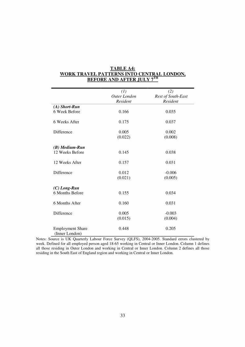
33

TABLE A4:

WORK TRAVEL PATTERNS INTO CENTRAL LONDON,

BEFORE AND AFTER JULY 7TH

(1)

Outer London

Resident

(2)

Rest of South-East

Resident

(A) Short-Run

6 Week Before

0.166 0.035

6 Weeks After

0.175 0.037

Difference 0.005

(0.022)

0.002

(0.008)

(B) Medium-Run

12 Weeks Before

0.145 0.038

12 Weeks After

0.157 0.031

Difference

0.012

(0.021)

-0.006

(0.005)

(C) Long-Run

6 Months Before

0.155 0.034

6 Months After

0.160 0.031

Difference

0.005

(0.015)

-0.003

(0.004)

Employment Share

(Inner London)

0.448 0.205

Notes: Source is UK Quarterly Labour Force Survey (QLFS), 2004-2005. Standard errors clustered by

week. Defined for all employed person aged 18-65 working in Central or Inner London. Column 1 defines

all those residing in Outer London and working in Central or Inner London. Column 2 defines all those

residing in the South East of England region and working in Central or Inner London.

34

TABLE A5:

SURVEY EVIDENCE ON COMMUNITY ATTITUDES,

INNER VERSUS OUTER LONDON

Question & Response

(1)

Inner London (%)

(2)

Outer London(%)

(1) As a result of the attacks have you

considered moving to live outside London or

not?

Yes

No

11

89

11

89

(2) How likely do you think it is London will

experience another attack in the near

future?

Very likely

Somewhat likely

Not very likely

Not at all likely

Don’t Know

36

43

11

4

6

48

37

8

3

4

(3) As a result of the attacks, have you spent

more or less time in Central London?

More time

Less time

Made No Difference

2

19

78

2

21

76

(4) Since the July attacks have you

personally or friends and relatives

experienced any hostility on the basis of

race or religion?

Yes: Verbal Abuse

Yes: Physical Abuse

Yes: Felt Under Suspicion or Stared At

Yes: Generally Felt Hostility

6

2

2

2

6

1

2

2

Source: IPSOS MORI Survey.

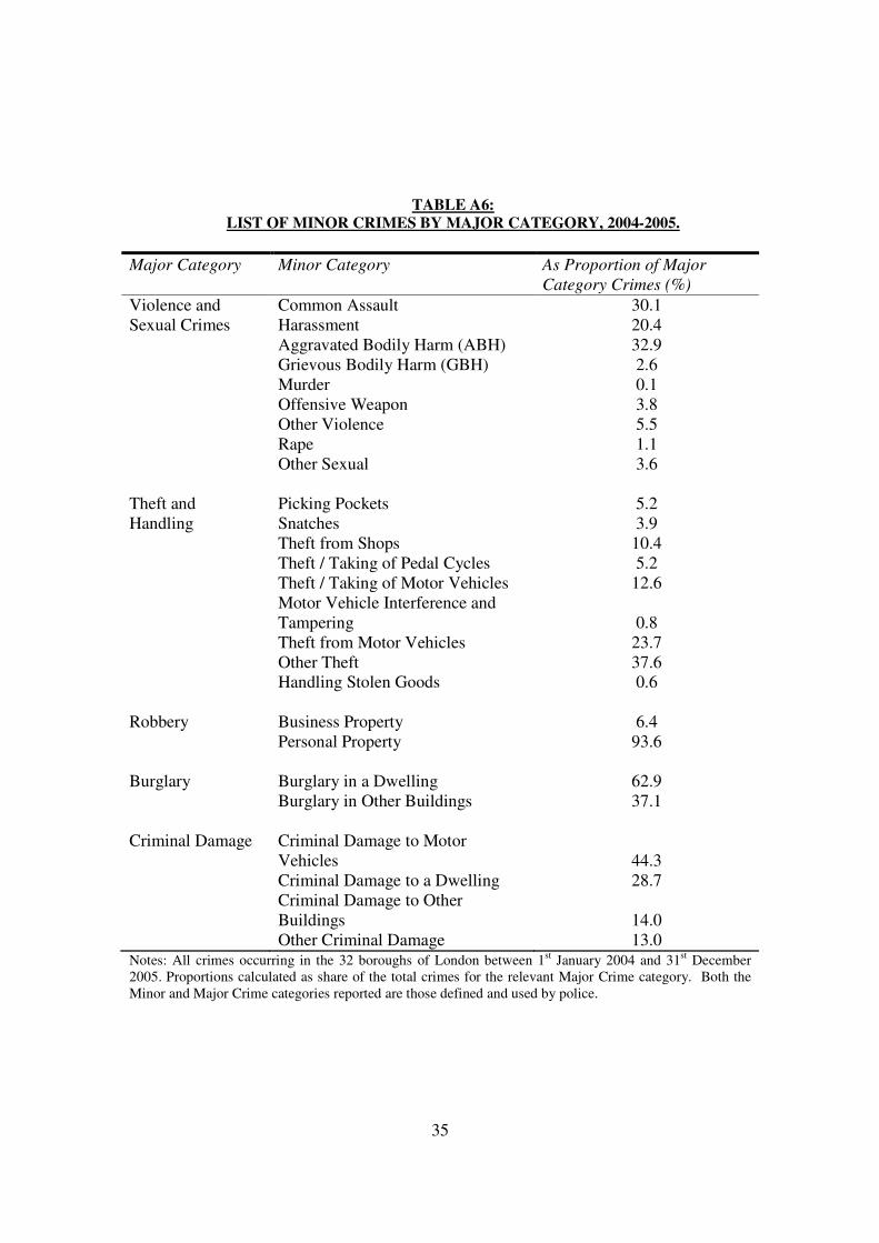
35

TABLE A6:

LIST OF MINOR CRIMES BY MAJOR CATEGORY, 2004-2005.

Major Category

Minor Category As Proportion of Major

Category Crimes (%)

Violence and

Sexual Crimes

Common Assault

Harassment

Aggravated Bodily Harm (ABH)

Grievous Bodily Harm (GBH)

Murder

Offensive Weapon

Other Violence

Rape

Other Sexual

30.1

20.4

32.9

2.6

0.1

3.8

5.5

1.1

3.6

Theft and

Handling

Picking Pockets

Snatches

Theft from Shops

Theft / Taking of Pedal Cycles

Theft / Taking of Motor Vehicles

Motor Vehicle Interference and

Tampering

Theft from Motor Vehicles

Other Theft

Handling Stolen Goods

5.2

3.9

10.4

5.2

12.6

0.8

23.7

37.6

0.6

Robbery Business Property

Personal Property

6.4

93.6

Burglary Burglary in a Dwelling

Burglary in Other Buildings

62.9

37.1

Criminal Damage

Criminal Damage to Motor

Vehicles

Criminal Damage to a Dwelling

Criminal Damage to Other

Buildings

Other Criminal Damage

44.3

28.7

14.0

13.0 Notes: All crimes occurring in the 32 boroughs of London between 1

st January 2004 and 31

st December

2005. Proportions calculated as share of the total crimes for the relevant Major Crime category. Both the

Minor and Major Crime categories reported are those defined and used by police.