Panel data models with spatially correlated error...

ARTICLE IN PRESS

Journal of Econometrics 140 (2007) 97–130

0304-4076/$ -

doi:10.1016/j

�CorrespoE-mail ad

www.elsevier.com/locate/jeconom

Panel data models with spatially correlatederror components

Mudit Kapoora, Harry H. Kelejianb, Ingmar R. Pruchab,�

aIndian School of Business (ISB), Gachibowli, Hyderabad 500 019, IndiabDepartment of Economics, University of Maryland, College Park, MD 20742, USA

Received in revised form 1 November 2004; accepted 5 September 2006

Available online 20 December 2006

Abstract

In this paper we consider a panel data model with error components that are both spatially and

time-wise correlated. The model blends specifications typically considered in the spatial literature

with those considered in the error components literature. We introduce generalizations of the

generalized moments estimators suggested in Kelejian and Prucha (1999. A generalized moments

estimator for the autoregressive parameter in a spatial model. International Economic Review 40,

509–533) for estimating the spatial autoregressive parameter and the variance components of the

disturbance process. We then use those estimators to define a feasible generalized least squares

procedure for the regression parameters. We give formal large sample results for the proposed

estimators. We emphasize that our estimators remain computationally feasible even in large samples.

r 2006 Elsevier B.V. All rights reserved.

JEL classification: C13; C21; C23

Keywords: Panel data model; Spatial model; Error component model

1. Introduction

This paper considers the estimation of spatial models from panel data. Spatial modelsare important tools in economics, regional science and geography in analyzing a widerange of empirical issues. Spatial interactions could be due to competition between cross

see front matter r 2006 Elsevier B.V. All rights reserved.

.jeconom.2006.09.004

nding author. Tel.: +1301 405 3499; fax: +1 301 405 3542.

dress: [email protected] (I.R. Prucha).

www.elsevier.com/locate/jeconom

dx.doi.org/10.1016/j.jeconom.2006.09.004

mailto:[email protected]

ARTICLE IN PRESSM. Kapoor et al. / Journal of Econometrics 140 (2007) 97–13098

sectional units, copy-cat policies, net work issues, spill-overs, externalities, regional issues,etc. Applications in the recent literature include, for example, the determinants of variousforms of productivity, various categories of local public expenditures, vote seeking and taxsetting behavior, population and employment growth, contagion problems, and thedeterminants of welfare expenditures.1 To facilitate the empirical analysis of spatial issuesthe formal development of estimation methods for spatial models has received increasingattention in recent years.2

In spatial models, interactions between cross sectional units are typically modelledin terms of some measure of distance between them. By far the most widely used spatialmodels are variants of the ones considered in Cliff and Ord (1973, 1981). One methodof estimation of these models is maximum likelihood (ML). However, even in itssimplest form, the ML estimation of Cliff–Ord-type models entails substantial computa-tional problems if the number of cross sectional units is large. Against this background,Kelejian and Prucha (1998) suggested an alternative instrumental variable estimationprocedure for these models, which is based on a generalized moments (GM) estimator of aparameter in the spatial autoregressive process. This GM estimator was suggested byKelejian and Prucha (1999) in an earlier paper.3 The procedures suggested in Kelejianand Prucha (1998, 1999) are computationally feasible even for large sample sizes.Also, Kelejian and Prucha gave formal large sample results for their procedures.4 As inmost of the spatial literature, they consider the case where a single cross section of data isavailable. Monte Carlo results in Das et al. (2003) suggest that both the GM and theinstrumental variable estimators are ‘‘virtually’’ as efficient as the corresponding MLestimators in small samples.The purpose of this paper is two-fold. First, we introduce generalizations of the GM

procedure in Kelejian and Prucha (1999) to panel data models involving a first orderspatially autoregressive disturbance term, whose innovations have an error componentstructure. In particular, we introduce three GM estimators which correspond to alternativeweighting schemes for the moments. Our specifications are such that the model’sdisturbances are potentially both spatially and time-wise autocorrelated, as well asheteroskedastic. These specifications merge those typically considered in the spatialliterature with those considered in the error component literature.Second, we define a feasible generalized least squares (FGLS) estimator for our model’s

regression parameters. This FGLS estimator is based on a spatial counterpart to the

1Some applications along these lines are, e.g., Audretsch and Feldmann (1996), Bernat (1996), Besley and Case

(1995), Bollinger and Ihlanfeldt (1997), Buettner (1999), Case (1991), Case et al. (1993), Dowd and LeSage (1997),

Holtz-Eakin (1994), LeSage (1999), Kelejian and Robinson (1997, 2000), Pinkse and Slade (1998), Pinkse et al.

(2002), Shroder (1995), and Vigil (1998).2Recent theoretical contributions include Baltagi and Li (2001a, b, 2004), Baltagi et al. (2003), Conley (1999),

Das et al. (2003), Kelejian and Prucha (1997, 1998, 1999, 2001, 2004), Lee (2001a, b, 2002, 2003, 2004), LeSage

(1997, 2000), Pace and Barry (1997), Pinkse and Slade (1998), Pinkse et al. (2002), and Rey and Boarnet (2004).

Classic references concerning spatial models are Anselin (1988), Cliff and Ord (1973, 1981), and Cressie (1993).3Due to publication lags, Kelejian and Prucha (1999) was published at a later date than Kelejian and Prucha

(1998), even though it was written at an earlier point in time.4The instrumental variable estimator suggested in Kelejian and Prucha (1998) is based on an approximation of

the ideal instruments. In recent paper, Lee (2003) and Kelejian et al. (2004) extend their approach towards the

ideal instruments.

ARTICLE IN PRESSM. Kapoor et al. / Journal of Econometrics 140 (2007) 97–130 99

Cochrane–Orcutt transformation, as well as transformations utilized in the estimation ofclassical error component models.5

We give formal results relating to our suggested procedures. Let T and N denote thesample sizes in the time and cross sectional dimensions, respectively. Then our analysiscorresponds to the case where T is fixed and N !1 and thus is geared towards sampleswhere N is large relative to T, as is frequently the case. In more detail, we first demonstratethat our generalizations of the GM approach lead to consistent estimators of theparameters of the disturbance process. Second, we formally derive the large sampledistribution of our FGLS estimators. In doing this we demonstrate that the parameters ofthe disturbance process are nuisance parameters. That is, we show that the true GLS andFGLS estimators have the same large sample distribution.

The model is specified and discussed in Section 2. Results relating to the GM proceduresare given in Section 3, and those relating to the FGLS estimators are given in Section 4.Monte Carlo results relating to our suggested GM estimators are given in Section 5. Section 6contains suggestions for future research. Technical details are relegated to Appendix A.

2. The model

2.1. Notation

In this section we specify the panel data model and then interpret its assumptions. Weassume that the data are available for spatial units i ¼ 1; . . . ;N for time periodst ¼ 1; . . . ;T . It proves helpful to introduce the following notation: Let AN ðtÞ be somematrix; then we denote the ði; jÞth element of AN ðtÞ as aijt;N . Similarly, if bN ðtÞ is a vector,then bit;N denotes the ith element of bN ðtÞ. If matrices or vectors do not depend on theindex t or N, then those indices are suppressed on the elements. If AN is a square matrix,then A�1N denotes the inverse of AN . If AN is singular, then A�1N should be interpreted as thegeneralized inverse of AN . Now let BN , NX1, be some sequence of kN � kN matrices withk some fixed positive integer. We will then say that the row and column sums of the(sequence of ) matrices BN are bounded uniformly in absolute value if there exists aconstant co1, that does not depend on N, such that

max1pipkN

XkN

j¼1

jbij;N jpc and max1pjpkN

XkN

i¼1

jbij;N jpc for all NX1.

As a point of interest, we note that the above condition is identical to the condition that thesequences of the maximum column sum matrix norms and maximum row sum matrixnorms of BN are bounded; cp. Horn and Johnson (1985, pp. 294–295). Finally, we denotethe unit vector of dimension S � 1 as eS.

2.2. Model specification

As remarked, in this paper we consider a linear regression panel data model that allowsfor the disturbances to be correlated over time and across spatial units. In particular, we

5See, e.g., Balestra and Nerlove (1966), Wallace and Hussain (1969), Amemiya (1971) and Nerlove (1971) for

seminal contributions to the literature on error components models. Early extensions to the systems case include

Baltagi (1980, 1981) and Prucha (1984, 1985). Baltagi (2001) and Hsiao (2003) provide excellent reviews.


assume that in each time period t ¼ 1; . . . ;T the data are generated according to thefollowing model:

yN ðtÞ ¼ X NðtÞbþ uN ðtÞ, (1)

where yNðtÞ denotes the N � 1 vector of observation on the dependent variable in period t,X N ðtÞ denotes the N � K matrix of observations on exogenous regressors in period t

(which may contain the constant term), b is the corresponding K � 1 vector of regressionparameters, and uN ðtÞ denotes the N � 1 vector of disturbance terms. We conditionalizeour model on the realized value of the regressors and so we will view X N ðtÞ, t ¼ 1; . . . ;T asmatrices of constants.A widely used approach to model spatial dependence is that of Cliff and Ord (1973,

1981). We follow this approach in modelling the disturbance process in each period as thefollowing first order spatial autoregressive process:

uN ðtÞ ¼ rW NuN ðtÞ þ eN ðtÞ, (2)

where W N is an N �N weighting matrix of known constants which does not involve t, r isa scalar autoregressive parameter, and eNðtÞ is an N � 1 vector of innovations in period t.For reasons of generality, we permit the elements of yNðtÞ, X N ðtÞ, uN ðtÞ, eN ðtÞ and W N todepend on N, that is, to form triangular arrays.Stacking the observations in (1) and (2) we have

yN ¼ X Nbþ uN , (3)

and

uN ¼ rðIT �W NÞuN þ eN , (4)

where yN ¼ ½y0N ð1Þ; . . . ; y

0NðTÞ�

0, X N ¼ ½X0Nð1Þ; . . . ;X

0N ðTÞ�

0, uN ¼ ½u0N ð1Þ; . . . ; u

0N ðTÞ�

0, andeN ¼ ½e0Nð1Þ; . . . ; e

0N ðTÞ�

0.To allow for the innovations to be correlated over time we assume the following error

component structure for the innovation vector eN :

eN ¼ ðeT � INÞmN þ nN , (5)

where mN represents the vector of unit specific error components, and nN ¼

½n0N ð1Þ; . . . ; n0NðTÞ�

0 contains the error components that vary over both the cross-sectionalunits and time periods. In scalar notation we have

eit;N ¼ mi;N þ nit;N . (6)

We note that the specification of eN corresponds to that of a classical one-way errorcomponent model; see, e.g., Baltagi (2001, p. 10). However, in contrast to much of theclassical error component literature we group the data by time periods rather than unitsbecause this grouping is more convenient for modelling spatial correlation via (2).We maintain the following assumptions.

Assumption 1. Let T be a fixed positive integer. (a) For all 1ptpT and 1pipN; NX1 theerror components nit;N are identically distributed with zero mean and variance s2n ,0os2nobno1, and finite fourth moments. In addition for each NX1 and 1ptpT ,1pipN the error components nit;N are independently distributed. (b) For all 1pipN,NX1 the unit specific error components mi;N are identically distributed with zero mean andvariance s2m, 0os2mobmo1, and finite fourth moments. In addition for each NX1 and


1pipN the unit specific error components mi;N are independently distributed. (c) Theprocesses fnit;Ng and fmi;Ng are independent.

Assumption 2. (a) All diagonal elements of W N are zero. (b) jrjo1: (c) The matrixIN � rW N is nonsingular.

2.3. Assumption implications

In light of (5) or (6) it is readily seen that Assumption 1 implies Eeit;N ¼ 0 and

Eðeit;Nejs;N Þ ¼

s2m þ s2n if i ¼ j; t ¼ s

s2m if i ¼ j; tas

0 otherwise

264375.

The innovations eit;N are autocorrelated over time, but are not spatially correlated acrossunits. In matrix notation we have EðeNÞ ¼ 0 and the variance–covariance matrix of eN is

Oe;N ¼ EðeNe0NÞ ¼ s2mðJT � IN Þ þ s2nINT

¼ s2nQ0;N þ s21Q1;N , ð7Þ

where s21 ¼ s2n þ Ts2m and

Q0;N ¼ IT �JT

T

� �� IN ,

Q1;N ¼JT

T� IN , (8)

and where JT ¼ eT e0T is a T � T matrix of unit elements. The matrices Q0;N and Q1;N arestandard transformation matrices utilized in the error component literature, with theappropriate adjustments implied by our adopted ordering of the data; compare, e.g.,Baltagi (2001, p. 10). The matrices Q0;N and Q1;N are symmetric and idempotent, andorthogonal to each other. Furthermore Q0;N þQ1;N ¼ INT , trðQ0;N Þ ¼ NðT � 1Þ, andtrðQ1;N Þ ¼ N. Also Q0;NðeT � INÞ ¼ 0 and Q1;N ðeT � IN Þ ¼ ðeT � IN Þ. Given theseproperties it is readily seen that

O�1e;N ¼ s�2n Q0;N þ s�21 Q1;N , (9)

which is important in that it facilitates the computation of O�1e;N even for large sample sizesN. As an illustration of the transformations implied by Q0;N and Q1;N consider thetransformed vectors Q0;NeN and Q1;NeN . It is readily seen that the ði; tÞth element of thosevectors is equal to eit;N � ei:;N and ei:;N , respectively, where ei:;N ¼ T�1

PTt¼1eit;N denotes the

sample mean taken over time corresponding to the ith unit. This shows that the Q0;N

transformation subtracts unit specific sample means from the original variable. Clearly,Q0;NeN ¼ Q0;NnN , i.e., the Q0;N transformation eliminates the unit specific errorcomponents.

Assumption 2, part (a) is a normalization of the model. The nonzero elements of theweighting matrix are typically specified to be those which correspond to units which arerelated in a meaningful way. Such units are said to be neighbors. Therefore, part (a) ofAssumption 2 also implies that no unit is a neighbor to itself. Note that although theelements of W N are assumed not to depend on t, we do allow them to form triangular


arrays. Among other things, this is consistent with models in which the weighting matrix isrow normalized and the number of neighbors a given unit may have depends on the samplesize. Parts (b) and (c) of Assumption 2 ensure that the model is closed in that it can beuniquely solved for the disturbance vector uN ðtÞ in terms of the innovation vector, eNðtÞ,and therefore for the dependent vector, yN ðtÞ, in terms of the exogenous regressor matrix,X N ðtÞ, and the innovation vector, eN ðtÞ. Specifically, we have in light of (1) and (2)

uN ðtÞ ¼ ðIN � rW N Þ�1eN ðtÞ,

yN ðtÞ ¼ X NðtÞbþ ðIN � rW N Þ�1eN ðtÞ,

or in stacked notation

uN ¼ ½IT � ðIN � rW NÞ�1�eN ,

yN ¼ X Nbþ ½IT � ðIN � rW NÞ�1�eN . (10)

It follows from (10) that the model disturbances are such that EðuN Þ ¼ 0 and EðuNu0N Þ ¼

Ou;N where

Ou;N ¼ ½IT � ðIN � rW NÞ�1�Oe;N ½IT � ðIN � rW 0

NÞ�1�. (11)

Clearly our assumptions imply that the model disturbances are, unless r ¼ 0, bothspatially and time-wise autocorrelated. In particular

E½uNðtÞu0N ðtÞ� ¼ ðs

2m þ s2nÞðIN � rW NÞ

�1ðIN � rW 0

NÞ�1.

We also note that, in general, the elements of ðIN � rW NÞ�1 will form triangular arrays in

that they will depend on the sample size, N. Consequently, the elements of uN and yN aswell as the elements of their variance covariance matrices will also form triangular arrays.Finally, we note that the model disturbances will generally be heteroskedastic.Anselin (1988, p. 153), and more recently Baltagi and Li (2004) and Baltagi et al. (2003),

have also considered error component specifications within the context of spatial models.6

We note that our specification differs somewhat from theirs in that we allow for spatialinteractions involving not only the error components vit;N , but also the unit specific errorcomponents, mi. We note that for T ¼ 1 our specification reduces to the standardCliff–Ord first order spatial autoregressive model.

3. A Generalised Moments Procedure

In the following we define three GM estimators of r; s2n and s2m, or equivalently of r, s2nand s21, since in our analysis T is fixed and N !1. These GM estimators are defined interms of six moment conditions. The first of these estimators provides initial estimates of r,s2n and s21, and is only based on a subset of the moment conditions. The initial estimates fors2n and s21 are then used in the formulation of the other two GM estimators. Morespecifically, our second GM estimator is based on all six moment conditions with thesample moments weighted by an approximation to the inverse of their variance covariance

6In contrast to this paper, which introduces generalizations of the GM estimation procedure for the spatial

autoregressive parameter and aims at establishing the asymptotic properties of the considered estimators, their

analysis had a different focus.


matrix.7 The third GM estimator is based on a simplified weighting scheme. The reason forconsidering the simplified weighting scheme is that the corresponding estimator is veryeasy to compute even in large samples. The considered GM estimators generalize, inessence, the GM estimators given in Kelejian and Prucha (1999) for the case of a singlecross section, which are based on three moment conditions, giving equal weight to eachsample moment. For notational convenience, let

uN ¼ ðIT �W N ÞuN ,

uN ¼ ðIT �W N ÞuN ,

eN ¼ ðIT �W NÞeN . (12)

3.1. Moment conditions

Given Assumptions 1 and 2 we demonstrate in Appendix A that, for (finite) TX2

E

1

NðT � 1Þe0NQ0;NeN

1


1


1

Ne0NQ1;NeN

1

Ne0NQ1;NeN

1

Ne0NQ1;NeN

2666666666666666666664

3777777777777777777775

¼

s2n

s2n1

NtrðW 0

NW NÞ

0

s21

s211

NtrðW 0

NW NÞ

0

2666666666664

3777777777775. (13)

Our three GM estimators of r, s2n , and s21 are based on these moment relationships. Theynaturally generalize the moment relationships introduced in Kelejian and Prucha (1998,1999) for a single cross section to the case of a panel of cross sections. If eN were observed,then e0NQ0;NeN=ðNðT � 1ÞÞ and e0NQ1;NeN=N represent the (unbiased) analysis of varianceestimators of s2v and s21, respectively; compare, e.g., Amemiya (1971). In case of a singlecross section, i.e., T ¼ 1, the innovations eN are i.i.d. with variance s21 (wheres21 ¼ s2v þ s2m), and in this case it is intuitively clear that we would only be able to identifys21 and not both s2v and s21. This is also reflected by the moment conditions (13) in that ifT ¼ 1 we have Q0;N ¼ 0 and the first three moment conditions become uninformative, andthe last three equations reduce to those considered in Kelejian and Prucha (1998, 1999). Inthe following we maintain TX2.

Towards defining our GM estimators we note that in light of (4) and (12)

eN ¼ uN � ruN ,

eN ¼ uN � ruN . (14)

7Under normality the approximation is perfect.


Substituting these expressions for eN and eN into (13) we obtain a system of six equationsinvolving the second moments of uN , uN and uN . This system involves r, s2n , and s21 and canbe expressed as

GN ½r; r2;s2n ;s21�0 � gN ¼ 0, (15)

where

GN ¼

g011;N g012;N g013;N 0

g021;N g022;N g023;N 0

g031;N g032;N g033;N 0

g111;N g112;N 0 g113;Ng121;N g122;N 0 g123;Ng131;N g132;N 0 g133;N

266666666664

377777777775; gN ¼

g01;Ng02;Ng03;Ng11;Ng12;Ng13;N

266666666664

377777777775,

and (i ¼ 0; 1)

gi11;N ¼

2

NðT � 1Þ1�iEu0NQi;NuN ; gi

12;N ¼�1

NðT � 1Þ1�iEu0NQi;NuN ;

gi21;N ¼

2

NðT � 1Þ1�iEu0

NQi;NuN ; gi22;N ¼

�1

NðT � 1Þ1�iEu0

NQi;NuN ;

gi31;N ¼

1

NðT � 1Þ1�iEðu0NQi;NuN þ u0NQi;NuN Þ; gi

32;N ¼�1


gi13;N ¼ 1; gi

1;N ¼1


gi23;N ¼

1

NtrðW 0

NW NÞ; gi2;N ¼

1


gi33;N ¼ 0; gi

3;N ¼1

NðT � 1Þ1�iEu0NQi;NuN :

The equations underlying our GM procedures are the sample counterparts to the sixequations in (15) based on estimated disturbances. In particular, let ~bN be an estimator ofb, and let

euN ¼ yN � X N~bN ,

euN ¼ ðIT �W NÞeuN ,

euN ¼ ðIT �W NÞeuN ¼ ðIT �W 2N ÞeuN . (16)

Then a sample analogue to (15) in terms of euN , euN and euN is

GN ½r;r2;s2n ; s21�0 � gN ¼ xNðr;s

2n ;s

21Þ, (17)


where

GN ¼

g011;N g0

12;N g013;N 0

g021;N g0

22;N g023;N 0

g031;N g0

32;N g033;N 0

g111;N g1

12;N 0 g113;N

g121;N g1

22;N 0 g123;N

g131;N g1

32;N 0 g133;N

266666666664

377777777775; gN ¼

g01;N

g02;N

g03;N

g11;N

g12;N

g13;N

266666666664

377777777775,

gi11;N ¼

2

NðT � 1Þ1�ieu0NQi;N

euN ; gi12;N ¼

�1


euN ;

gi21;N ¼

2


euN ; gi22;N ¼

�1


euN ;

gi31;N ¼

1

NðT � 1Þ1�iðeu0NQi;N

euN þ eu0NQi;NeuN Þ; gi

32;N ¼�1


euN ;

gi13;N ¼ 1; gi

1;N ¼1

NðT � 1Þ1�ieu0NQi;NeuN ;

gi23;N ¼

1

NtrðW 0

NW NÞ; gi2;N ¼

1


euN ;

gi33;N ¼ 0; gi

3;N ¼1


euN ;

where xN ðr;s2n ;s21Þ is a vector of residuals.

Towards defining our GM procedures it proves helpful to observe that the first threeequations in (15) do not involve s21, while the last three do not involve s2v . In particular, letG0

N ¼ ðg0ij;N Þi; j¼1;2;3, and G1

N ¼ ðg1ij;N Þi; j¼1;2;3. Then (15) can be rewritten as

G0N ½r;r

2; s2n �0 � g0N ¼ 0,

G1N ½r;r

2; s21�0 � g1N ¼ 0. (18)

Analogously let G0N ¼ ðg

0ij;NÞi; j¼1;2;3, and G1

N ¼ ðg1ij;N Þi; j¼1;2;3. Then (17) can be rewritten as

G0N ½r;r

2;s2n �0 � g0

N ¼ x0N ðr; s2nÞ,

G1N ½r;r

2;s21�0 � g1

N ¼ x1N ðr; s21Þ, (19)

where xN ðr;s2n ;s21Þ ¼ ½x

0N ðr;s

2nÞ0; x1Nðr;s

21Þ0�0.

3.2. Additional assumptions

We need the following additional assumptions.


Assumption 3. The elements of X N are bounded uniformly in absolute value by kxo1.
Furthermore, for i ¼ 0; 1, the matrices
Mixx ¼ lim

N!1

1

NTX �N ðrÞ

0Qi;NX �N ðrÞ0, (20)

with X �NðrÞ ¼ ½IT � ðIN � rW NÞ�X N , are finite, and the matrices

limN!1

1

NTX 0NX N ; lim

N!1

1

NTX �NðrÞ

0X �N ðrÞ; limN!1

1

NTX �NðrÞ

0O�1e;NX �NðrÞ (21)

are finite and nonsingular.

Assumption 4. The row and column sums of W N and PN ðrÞ ¼ ðIN � rW NÞ�1are bounded

uniformly in absolute value by, respectively, kwo1 and kpo1 where kp may depend on r.

Assumption 5. The smallest eigenvalues of ðG0NÞ0ðG0

N Þ and ðG1N Þ0ðG1

NÞ are bounded awayfrom zero, i.e., lmin½ðGi

NÞ0ðGi

N Þ�Xl�40 for i ¼ 1; 2, where l� may depend on r, s2n and s21.

Conditions like those maintained in Assumption 3 are typical in large sample analysis,see e.g., Kelejian and Prucha (1998, 1999). The large sample properties of the generalizedleast squares (GLS) estimator of b considered below will involve the limit ofðNT Þ�1X 0NO

�1u;NX N . It follows from (11) that

O�1u;N ¼ ½IT � ðIN � rW 0NÞ�O

�1e;N ½IT � ðIN � rW NÞ�. (22)

Recalling the expression for O�1e;N in (9) and utilizing Assumption 3 it then follows that:

limN!1ðNT Þ�1X 0NO

�1u;NX N ¼ lim

N!1

1

NTX �N ðrÞ

0O�1e;NX �N ðrÞ

¼ s�2n M0xx þ s�21 M1

xx. ð23Þ

Assumption 4 has two parts. The first relates directly to the weighting matrix andrestricts the extent of neighborliness of the cross sectional units. In practice this part shouldbe satisfied if each unit has only a limited number of neighbors, and is itself a neighbor to alimited number of other units—i.e., W N is sparse. It will also be satisfied if W N is notsparse, but its elements decline with a distance measure that increases sufficiently rapidly asthe sample increases. The second component of Assumption 4 relates to ðIN � rW N Þ

�1.From (11) and the subsequent discussion, the variance covariance matrix of thedisturbance vector uNðtÞ is seen to be proportional to ðIN � rW N Þ

�1ðIN � rW 0

N Þ�1. The

second component of Assumption 4 implies that row and column sums of this matrix arebounded uniformly in absolute value, since this property is preserved under matrixmultiplication; see Remark A2 in Appendix A. Assumption 4 thus restricts the degree ofcross sectional correlation between the model disturbances. For perspective, we note thatin virtually all large sample theory it is necessary to restrict the degree of permissiblecorrelations, see e.g., Amemiya (1985, Chapters 3 and 4) or Potscher and Prucha (1997,Chapters 5 and 6).Assumption 5 ensures identifiable uniqueness of the parameters r, s2n , and s21.

As demonstrated in Appendix A, it implies that also the smallest eigenvalue of G0NGN


is bounded away from zero. A similar assumption was made in Kelejian and Prucha(1998).8

3.3. The GM estimators

As remarked, we consider three GM estimators of r, s2n , and s21. The first set of GMestimators will be denoted as ~rN , ~s

2n;N , and ~s21;N . These estimators are intended as initial

estimators and will be referred to as such. They are based only on a subset of the momentconditions in (15) or (18). In particular, the estimators ~rN and ~s2n;N use only the first threesample moments to estimate r and s2n , giving equal weights to each of those moments.They are defined as the unweighted nonlinear least squares estimators based on the firstthree equations in (17) or (19):

ð ~rN ; ~s2n;N Þ ¼ arg minfx0N ðr; s

2nÞ0x0N ðr;s

2nÞ; r 2 ½�a; a�; s2n 2 ½0; b�g, (24)

where aX1, bXbn. By assumption jrjo1. If the bound a defining the optimization space issufficiently large, then ~rN is essentially the unconstrained nonlinear least squares estimatorof r.9 The assumption of a compact optimization space is standard in the literature onnonlinear estimation; see, e.g., Gallant and White (1988) and Potscher and Prucha (1997).Lee (2004) also maintains a compactness assumption in deriving the asymptotic propertiesof the ML estimator for the spatial autoregressive parameter in a cross section framework.We note that in contrast to the ML estimator, the objective function of the GM estimatorremains well defined for values r for which IN � rW N is singular.

For clarity we note that x0N ðr;s2nÞ ¼ G0

N ½r;r2; s2n �

0 � g0N . The elements of the G0

N and g0N

are observed. The estimator in (24) can thus be computed from a nonlinear regression of

the ‘‘dependent’’ variable g0N on the three ‘‘independent’’ variables composing G0

N , based

on three observations on those variables. The nonlinearity arises because of the restriction

between the first two elements of the parameter vector ðr;r2;s2nÞ. It follows that the

procedure described in (24) can be implemented in any software package which contains anonlinear least squares option. It should also be clear that an over-parameterized ordinary

least squares (OLS) estimator can be obtained as ½ðG0N Þ0ðG0

NÞ��1ðG0

NÞ0g0

N . In their study

dealing with only a single cross section, Kelejian and Prucha (1999) found that their over-parameterized OLS estimator was less efficient than their nonlinear least squares estimator,and so we will not further consider this estimator here.

Given ~rN and ~s2n;N we can estimate s21 from the fourth moment condition as

~s21;N ¼1

NðeuN � ~rN

euN Þ0Q1;NðeuN � ~rN

euNÞ

¼ g11;N � g1

11;N ~rN � g112;N ~r

2N . ð25Þ

The fourth moment condition corresponds to the fourth equation in (17) or (19). We notethat the estimator ~s21;N has the interpretation of an analysis of variance estimator for s21based on the estimated innovations ee ¼ euN � ~rN

euN .

8For a further discussion of the identifiable uniqueness assumption in nonlinear estimation see, e.g., Gallant

and White (1988) and Potscher and Prucha (1997).9We note that in small samples we may obtain estimates ~rN with j ~rN jX1. To force the estimator into the

interval ð�1; 1Þ one may consider the reparameterization r ¼ tan h ðKÞ and optimize w.r.t. k.


Theorem 1 below establishes the consistency of the GM estimators ~rN , ~s2n;N , and ~s21;N

defined by (24) and (25). The proof of the theorem is given in Appendix A.

Theorem 1. Suppose Assumptions 1–5 hold. Then, if ~bN is a consistent estimator of b, the

GM estimators ~rN ; ~s2n;N ; ~s

21;N are consistent for r;s2n ;s

21 i.e.,

ð ~rN ; ~s2n;N ; ~s

21;NÞ!

Pðr;s2n ;s

21Þ as N !1.

We show in Appendix A that Assumptions 1–4 imply that the OLS estimator of bcorresponding to (3) is consistent, and thus it can be used to calculate the estimateddisturbances employed in the GM procedure described by (24) and (25).It is well known from the literature on generalized method of moments estimators that for

purposes of asymptotic efficiency it is optimal to use the inverse of the (properly normalized)variance covariance matrix of the sample moments at the true parameter values as aweighting matrix. In our case the sample moments at the true parameter value are given bythe first vector in (13) with the expectations operator suppressed. In Appendix A we derivethe following expression for the variance covariance matrix of those sample moments, aftermultiplication by N:

XN ¼

1

T � 1s4n 0

0 s41

264375� TW , (26)

where

TW ¼

2 2 trW 0

NW N

N

� �0

2 trW 0

NW N

N

� �2 tr

W 0NW NW 0

NW N

N

� �tr

W 0NW N ðW

0N þW NÞ

N

� �

0 trW 0

NW N ðW0N þW NÞ

N

� �tr

W NW N þW 0NW N

N

� �

266666666664

377777777775.

The above variance covariance matrix was derived under the assumption that theinnovations are normally distributed. Hence the use of this matrix will not be strictlyoptimal in the absence of normality. However this matrix has the advantage of relativesimplicity. In the absence of normality the variance covariance matrix in (26) can be viewedas an approximation to the more complex true variance covariance matrix. We note thatour consistency results below do not depend upon the normality assumption.The variance covariance matrix XN depends on s2n and s21, and is hence unobserved. It

seems natural to define our estimator ~XN to be identical to XN except that s4n and s41 arereplaced by estimators. Clearly ~XN is a consistent estimator for XN , if the estimators for s2nand s21 are consistent. Our second GM estimator is then defined as the nonlinear leastsquares estimators based on (17) with the sample moments weighted by ~X

�1

N :

ðrN ; s2n;N ; s

21;NÞ ¼ arg minfxN ðr;s

2n ;s

21Þ0 ~X�1

N xNðr;s2n ;s

21Þ,

r 2 ½�a; a�; s2n 2 ½0; b�; s21 2 ½0; c�g, ð27Þ


where aX1, bXbn, cXTbm þ bn. We refer to this estimator in the following as the weightedGM estimator.

A discussion analogous to that after the definition of the initial GM estimator alsoapplies here. In particular, the weighted GM estimator defined in (27) can be computed byrunning a weighted nonlinear regression of gN on GN with ~X

�1

N as the weights matrix. Inlight of Theorem 1 above we can use, in particular, the initial GM estimators ~s2n;N and ~s21;Nto construct a consistent estimator ~XN for XN .

The next theorem establishes the consistency of the weighted GM estimator defined by(27). The proof of the theorem is given in Appendix A.

Theorem 2. Suppose Assumptions 1–5 hold and the smallest and largest eigenvalues of the

matrices X�1N satisfy 0ol�plminðX�1N ÞplmaxðX�1N Þpl��o1. Suppose furthermore that ~bN

and ~XN are consistent estimators of b and XN , respectively. Then, the GM estimators

rN ; s2n;N ; s

21;N defined by (27) are consistent for r;s2n ; s

21, i.e.,

ðrN ; s2n;N ; s

21;NÞ!

Pðr; s2n ; s

21Þ as N !1.

The assumptions relating to the eigenvalues of X�1N together with Assumption 5 ensurethe identifiably uniqueness of the parameters r; s2n ; s

21. They also ensure that the elements

of X�1N are Oð1Þ.The third GM estimator considered here is motivated mostly by computational

considerations. To calculate the estimator ~XN considered above we have to compute theelements of TW . While TW can be computed accurately even for large n, nevertheless it isreadily seen that the computation of, in particular, the ð2; 2Þ element of that matrixinvolves a computational count of up to Oðn3Þ. Thus it seems of interest to also consider analternative estimator that is computationally simpler. Let

UN ¼

1

T � 1s4n 0

0 s41

264375� I3 (28)

and let ~UN be the corresponding estimator where s2n and s21 are replaced by estimators. Thatis, UN and ~UN have the same form as XN and ~XN , except that TW is replaced by the identitymatrix I3. Our third GM estimator is then defined as the nonlinear least squares estimatorsbased on (17) where the sample moments are weighted by ~U �1N :

ð �rN ; �s2n;N ; �s

21;NÞ ¼ arg minfxNðr; s

2n ;s

21Þ0 ~U �1N xN ðr; s

2n ; s

21Þ

r 2 ½�a; a�; s2n 2 ½0; b�; s21 2 ½0; c�g, ð29Þ

where, again, aX1, bXbn, cXTbm þ bn. We refer to this estimator as the partially weightedGM estimator. It places the same weight on each of the first three moment equations, andthe same weight on each of the last three moment equations, but the weight given to thefirst three moment equations is different than that given to the last three momentequations. This weighting scheme is motivated by the estimator considered in Kelejian andPrucha (1998, 1999), which is based on three equally weighted moment equations. Thosestudies report that the estimator exhibits a small sample behavior that is quite similar tothe ML estimator both for a set of idealized and real world weighting matrices W N . Thissuggest that, at least for some matrices W N ; the weighting scheme implied by T�1W ascompared to the identity matrix is of lesser importance. The Monte Carlo results given


below provide some support for this conjecture also in the present context of panel data. Inlight of Theorem 1 above we can use again the initial GM estimators ~s2n;N and ~s21;N toconstruct a consistent estimator ~UN for UN .The next theorem establishes the consistency of the partially weighted GM estimator

defined by (29). The proof of the theorem is given in Appendix A.

Theorem 3. Suppose Assumptions 1–5 hold. Suppose furthermore that ~bN and ~U �1N are

consistent estimators of b and UN , respectively. Then, the GM estimators �rN ; �s2n;N ; �s

21;N

defined by (29) are consistent for r;s2n ;s21, i.e.,

ð �rN ; �s2n;N ; �s

21;NÞ!

Pðr;s2n ;s

21Þ as N !1.

A more extreme simplified weighting scheme would be to give equal weight to all sixmoment equations. The corresponding GM estimator is also readily seen to be consistent.However, preliminary Monte Carlo results suggest that the small sample behavior of thisestimator can be substantially worse than that of the other three estimators, and hence wedo not further consider this estimator in this study.

4. Spatial GLS estimation

Consider again the regression model in (3)–(5). The true GLS estimator of b is given by

bGLS;N ¼ fX0N ½O

�1u;N ðr;s

2n ;s

21Þ�X Ng

�1X 0N ½O�1u;N ðr;s

2n ;s

21Þ� yN

¼ fX �N ðrÞ0½O�1e;N ðs

2n ;s

21Þ�X

�NðrÞg

�1X �NðrÞ0½O�1e;Nðs

2n ; s

21Þ� y

�NðrÞ, ð30Þ

where

y�N ðrÞ ¼ ½IT � ðIN � rW N Þ� yN ,

X �NðrÞ ¼ ½IT � ðIN � rW NÞ�X N , (31)

and where we have denoted the explicit dependence of O�1u;N and O�1e;N on r and/or s2n ands21. The second expression in (30) is obtained by utilizing the expression for Ou;N given in(11). The variables y�NðrÞ and X �NðrÞ can be viewed as the result of a spatialCochrane–Orcutt type transformation of the original model. More specifically, pre-multiplication of (3) and (4) with IT � ðIN � rW N Þ yields

10

y�N ðrÞ ¼ X �N ðrÞbþ eN . (32)

In light of (9) and the properties of Q0;N and Q1;N we have O�1e;N ¼ O�1=2e;N O�1=2e;N with

O�1=2e;N ¼ s�1n Q0;N þ s�11 Q1;N . (33)

Guided by the classical error component literature, we note that a convenient way ofcomputing the GLS estimator bGLS;N is to further transform the model in (32) bypremultiplying it by O�1=2e;N , or equivalently by

snO�1=2e;N ¼ INT � yQ1;N , (34)

10This is, of course, equivalent to premultiplying (1) and (2) in each period t by ðIN � rW N Þ and then stacking

the data.


where y ¼ 1� sn=s1. The GLS estimator of b is then identical to the OLS estimator of bcomputed from the resulting transformed model. We note that the transformation basedon (34) simply amounts to subtracting from each variable its sample mean over timemultiplied by y.

Let �rN ; �s2n;N ; �s

21;N be estimators of r;s2n;N ; s

21;N . The corresponding feasible GLS

estimator of b, say bFGLS;N , is then obtained by replacing r;s2n;N ;s21;N by those estimators

in the expression for the GLS estimator, i.e.,

bFGLS;N ¼ fX�Nð �rN Þ

0½O�1e;N ð �s

2n;N ; �s

21;NÞ�X

�N ð �rN Þg

�1

� X �N ð �rNÞ0½O�1e;Nð �s

2n;N ; �s

21;N Þ� y

�N ð �rNÞ. ð35Þ

This estimator can again be computed conveniently as the OLS estimator aftertransforming the model in a way analogously to what was described for the GLSestimator.

The next theorem establishes consistency and asymptotic normality of the true andfeasible GLS estimators. The proof of the theorem is given in Appendix A.

Theorem 4. Given Assumptions 1–4 hold:

(a)
Then
ðNT Þ1=2½bGLS;N � b�!D

Nf0;Cg as N !1,

with

C ¼ ½s�2n M0xx þ s�21 M1

xx��1.

(b)
If �rN ; �s2n;N ; �s
21;N are (any) consistent estimators of r, s2n , s

21, then

ðNT Þ1=2½bGLS;N � bFGLS;N �!P0 as N !1.

(c)
Furthermore,
�CN �C!P0 as N !1,

where

�CN ¼1

NTX �N ð �rN Þ

0½O�1e;N ð �s

2n;N ; �s

21;N Þ�X

�N ð �rNÞ

� ��1.

Part (a) implies that the true GLS estimator, bGLS;N , is consistent and asymptoticallynormal. Part (b) implies that if the feasible GLS estimator, bFGLS;N , is based on anyconsistent estimators of r, s2n , s

21, then bGLS;N and bFGLS;N are asymptotically equivalent,

and hence bFGLS;N is also consistent and asymptotically normal with the same asymptoticdistribution as bGLS;N . Therefore, r, s

2n , s

21 are ‘‘nuisance’’ parameters. Together with part

(c), these results suggest that small sample inferences can be based on the approximation

bFGLS;N �:

Nðb; ðNT Þ�1 �CNÞ.


In Theorems 2 and 3 we establish the consistency of the weighted and partially weightedGM estimators for r, s2n , and s21, respectively. Therefore, these estimators can be used toconstruct the feasible GLS estimator considered in Theorem 4.

5. A Monte Carlo investigation

In the following we report on a small Monte Carlo study of the small sample propertiesof the estimators suggested in this paper. We consider the three suggested GM estimatorsof the spatial autoregressive parameter r and variances s2m and s21, and correspondingfeasible GLS estimators for b. We also consider iterated versions of these estimators. Forpurposes of comparison, we also consider the ML estimator of these parameters. A largerMonte Carlo study relating to a wider set of experiments than those described below is leftfor future research.In all of our Monte Carlo experiments N ¼ 100 and T ¼ 5. The data are generated

according to (3)–(5) with the regressor matrix containing two regressors x1 and x2 withcorresponding parameters b1 and b2. In our illustrative experiments we take x1 to be theconstant term. The observations on x2 corresponds to per capita income (measured in$1000) in 100 contiguous counties in Virginia over the periods 1996–2000. The parametersb1 and b2 are taken to be equal to one. We assume that both of the error components, mN

and nN , are normally distributed. The generation of the disturbance vector uN requiresthe specification of s2m, s

2n , r, and the weighting matrix W N . In all of our Monte Carlo

experiments s2m ¼ s2n ¼ 1 and thus s21 ¼ 6.11 As in Kelejian and Prucha (1999), we considerseven values of r, namely �0:9, �0:5, �0:25, 0, 0:25, 0:5, and 0:9. Also, as in the earlierstudy we consider three weighting matrices which essentially differ in their degrees ofsparseness. The first matrix is such that its ith row, 1oioN, has nonzero elements inpositions i þ 1 and i � 1 so that the ith element of uN ðtÞ, 1oioN, is directly related tothe one immediately after it, and the one immediately before it. This matrix is definedin a circular world so that the nonzero elements in rows 1 and N are, respectively, inpositions (1,2), ð1;NÞ and ðN ; 1Þ, ðN ;N � 1Þ. This matrix is row normalized so that all ofit’s nonzero elements are equal to 1

2. As in Kelejian and Prucha (1999, p. 520) we refer to

this specification of the weighting matrix as ‘‘1 ahead and 1 behind.’’ The other twoweighting matrices we consider are defined in a corresponding way as 3 ahead and 3behind, and 5 ahead and 5 behind. The nonzero elements in these matrices are,respectively, 1

6and 1

10. In Tables 1–5, below we reference these three weighting matrices by

J ¼ 2; 6; 10, where J is the number of nonzero elements in a given row. To summarize, ourexperimental design contains 21 cases, which result from 7 selections of r and 3specifications of the weighting matrix. We have also calculated R2 values (obtained from asimple least squares regression of y on the regressors). The median R2 values for respectiveexperiments ranges between 0.61–0.95, 0.77–0.95 and 0.83–0.95 for J ¼ 2, 6 and 10,respectively.Recall that ð ~r; ~s2n ; ~s

2nÞ, ðr; s

2n ; s

21Þ, and ð �r; �s

2n ; �s

21Þ, defined in (24), (27), and (29) denote the

initial (unweighted), the weighted and the partially weighted GM estimators for ðr;s2n ;s21Þ,

11We considered other values of the ratio s2m=s2n but the results were qualitatively similar to those reported

below for the case s2m ¼ s2n ¼ 1. Again, to conserve space these results are not reported, but are available upon

request.

ARTICLE IN PRESS

Table 1

RMSEs of the estimators of r

Parameter values RMSE

J r rML ~r r �r ~rð1Þ rð1Þ �rð1Þ

2 �0.9 0.0111 0.0191 0.0149 0.0182 0.0150 0.0122 0.0133

2 �0.5 0.0344 0.0416 0.0354 0.0355 0.0409 0.0351 0.0353

2 �0.25 0.0420 0.0496 0.0422 0.0419 0.0493 0.0415 0.0421

2 0 0.0445 0.0522 0.0446 0.0437 0.0520 0.0450 0.0444

2 0.25 0.0420 0.0499 0.0431 0.0416 0.0502 0.0431 0.0420

2 0.5 0.0350 0.0420 0.0359 0.0354 0.0421 0.0363 0.0354

2 0.9 0.0111 0.0157 0.0131 0.0142 0.0158 0.0125 0.0132

6 �0.9 0.0857 0.1088 0.0872 0.0975 0.1080 0.0872 0.0979

6 �0.5 0.0902 0.1037 0.0861 0.0925 0.1051 0.0890 0.0938

6 �0.25 0.0846 0.0962 0.0825 0.0865 0.0989 0.0826 0.0873

6 0 0.0757 0.0869 0.0750 0.0769 0.0883 0.0748 0.0776

6 0.25 0.0653 0.0739 0.0648 0.0652 0.0745 0.0649 0.0657

6 0.5 0.0503 0.0572 0.0504 0.0498 0.0573 0.0511 0.0499

6 0.9 0.0160 0.0188 0.0175 0.0171 0.0188 0.0171 0.0166

10 �0.9 0.1336 0.1563 0.1431 0.1458 0.1718 0.1402 0.1530

10 �0.5 0.1265 0.1489 0.1302 0.1317 0.1564 0.1301 0.1355

10 �0.25 0.1184 0.1360 0.1187 0.1186 0.1410 0.1212 0.1213

10 0 0.1049 0.1197 0.1049 0.1032 0.1223 0.1068 0.1034

10 0.25 0.0879 0.1007 0.0844 0.0848 0.1005 0.0849 0.0857

10 0.5 0.0657 0.0753 0.0646 0.0637 0.0753 0.0641 0.0646

10 0.9 0.0207 0.0243 0.0206 0.0216 0.0241 0.0205 0.0211

Column averages 0.0641 0.0756 0.0647 0.0660 0.0766 0.0648 0.0666

rML is the maximum likelihood estimator; ~r the initial (unweighted) GM estimator; r the weighted GM estimator;

�r the partially weighted GM estimator; ~rð1Þ the initial (unweighted) GM estimator, iterated once; rð1Þ the weightedGM estimator, iterated once; and �rð1Þ the partially weighted GM estimator, iterated once.

N ¼ 100, T ¼ 5, and ðs2m;s2n ;s

21; b1;b2Þ ¼ ð1; 1; 6; 1; 1Þ.

M. Kapoor et al. / Journal of Econometrics 140 (2007) 97–130 113

respectively.12 These estimators are computed from OLS residuals. Based on the respective

sets of GM estimators for ðr;s2n ; s21Þ we compute feasible GLS estimators for b1 and b2 by

substituting into the formula for the feasible GLS estimator in (35) the respective sets of

GM estimators for ðr;s2n ;s21Þ. We denote the corresponding feasible GLS estimators as

~bi;FGLS, bi;FGLS and�bi;FGLS, i ¼ 1; 2, respectively. We also compute iterated version of these

estimators. Towards computing these iterated estimators we first compute feasible GLS

residuals corresponding to ~bi;FGLS, bi;FGLS and �bi;FGLS, i ¼ 1; 2, respectively. We then use

those residuals to compute new sets of the initial (unweighted), the weighted, and the

partially weighted GM estimators for ðr;s2n ;s21Þ. These estimators will be denoted as

ð ~rð1Þ; ~s2ð1Þn ; ~s2ð1Þn Þ, ðrð1Þ; s2ð1Þn ; s2ð1Þ1 Þ, and ð �r

ð1Þ; �s2ð1Þn ; �s2ð1Þ1 Þ.13 In computing the matrices ~XN and

12For simplicity of notation we drop the index corresponding to the sample size here and in the following.13We have called the GM estimators ð ~r; ~s2n ; ~s

2n Þ, which correspond to the first four unweighted moment

conditions, the initial (unweighted) GM estimators. In slight abuse of language, we call the GM estimators

ð ~rð1Þ; ~s2ð1Þn ; ~s2ð1Þn Þ, which correspond to the first four unweighted moment conditions based on feasible GLS

disturbances corresponding to ~bi;FGLS, the once iterated initial (unweighted) GM estimators.

ARTICLE IN PRESS

Table 2

RMSEs of the estimators of s2v


J r s2;MLv ~s2v s2v �s2v ~s2ð1Þv s2ð1Þv �s2ð1Þv

2 �0.9 0.0761 0.1238 0.1046 0.1231 0.0846 0.0772 0.0846

2 �0.5 0.0734 0.0749 0.0728 0.0735 0.0736 0.0732 0.0736

2 �0.25 0.0730 0.0739 0.0730 0.0735 0.0737 0.0738 0.0737

2 0 0.0725 0.0720 0.0724 0.0719 0.0725 0.0723 0.0725

2 0.25 0.0726 0.0748 0.0731 0.0749 0.0748 0.0731 0.0748

2 0.5 0.0742 0.0777 0.0753 0.0758 0.0776 0.0751 0.0776

2 0.9 0.0756 0.0876 0.0798 0.0836 0.0864 0.0790 0.0864

6 �0.9 0.0774 0.0767 0.0743 0.0738 0.0764 0.0756 0.0762

6 �0.5 0.0743 0.0735 0.0733 0.0734 0.0755 0.0743 0.0738

6 �0.25 0.0737 0.0730 0.0727 0.0734 0.0746 0.0731 0.0739

6 0 0.0732 0.0739 0.0741 0.0739 0.0732 0.0731 0.0731

6 0.25 0.0733 0.0730 0.0734 0.0731 0.0733 0.0733 0.0735

6 0.5 0.0727 0.0722 0.0729 0.0729 0.0724 0.0726 0.0730

6 0.9 0.0740 0.0743 0.0735 0.0746 0.0734 0.0727 0.0747

10 �0.9 0.0739 0.0751 0.0755 0.0745 0.0751 0.0740 0.0758

10 �0.5 0.0732 0.0725 0.0732 0.0721 0.0738 0.0736 0.0736

10 �0.25 0.0730 0.0730 0.0728 0.0723 0.0745 0.0736 0.0733

10 0 0.0732 0.0739 0.0737 0.0735 0.0737 0.0733 0.0733

10 0.25 0.0734 0.0731 0.0736 0.0735 0.0729 0.0735 0.0734

10 0.5 0.0723 0.0714 0.0720 0.0722 0.0713 0.0719 0.0722

10 0.9 0.0727 0.0720 0.0731 0.0725 0.0723 0.0727 0.0729

Column averages 0.0737 0.0768 0.0752 0.0763 0.0750 0.0739 0.0750

s2;MLv is the maximum likelihood estimator; ~s2v the initial (unweighted) GM estimator; s2v the weighted GM

estimator; �s2v the partially weighted GM estimator; ~s2ð1Þv the initial (unweighted) GM estimator, iterated once; s2ð1Þv

the weighted GM estimator, iterated once; and �s2ð1Þv the partially weighted GM estimator, iterated once.

N ¼ 100, T ¼ 5, and ðs2m;s2n ; s

21;b1;b2Þ ¼ ð1; 1; 6; 1; 1Þ.

M. Kapoor et al. / Journal of Econometrics 140 (2007) 97–130114

~UN that enter into the objective function for the weighted and the partially weighted GM

estimators we use ðs2n ; s21Þ, and ð �s

2n ; �s

21Þ. Using the (once) iterated initial (unweighted), the

weighted, and the partially weighted GM estimators for ðr; s2n ;s21Þ we compute the (once)

iterated feasible GLS estimators which we denote as ~bð1Þi;FGLS, bð1Þi;FGLS and �b

ð1Þ

i;FGLS, i ¼ 1; 2.

Table 1 contains results on a measure of dispersion relating to the small sampledistributions of the GM estimators ~r, r, �r, the corresponding iterated GM estimators, andthe ML estimator, rML, for each of 21 cases. Our adopted measure of dispersion is closelyrelated to the standard measure of the root mean squared error (RMSE), but is based onquantiles rather than moments, because, unlike moments, quantiles are assured to exit. Forease of presentation, we also refer to our measure as the RMSE. It is defined as

RMSE ¼ bias2 þIQ

1:35

� �2" #1=2,

where bias is the difference between the median and the true value of r, and IQ is theinterquantile range defined as c1 � c2, where c1 is the 0:75 quantile and c2 is the 0:25

ARTICLE IN PRESS

Table 3

RMSEs of the estimators of s21


J r s2;ML1

~s21 s21 �s21 ~s2ð1Þ1 s2ð1Þ1 �s2ð1Þ1

2 �0.9 0.8269 1.3474 1.2562 1.3364 0.8587 0.8217 0.8374

2 �0.5 0.8222 0.8340 0.8267 0.8269 0.8450 0.8168 0.8401

2 �0.25 0.8298 0.8445 0.8270 0.8431 0.8381 0.8307 0.8528

2 0 0.8357 0.8288 0.8298 0.8377 0.8267 0.8300 0.8454

2 0.25 0.8374 0.8336 0.8409 0.8494 0.8341 0.8353 0.8527

2 0.5 0.8411 0.8098 0.8322 0.8446 0.8312 0.8445 0.8679

2 0.9 0.8350 1.1895 1.1898 1.2240 0.8497 0.8320 0.8664

6 �0.9 0.8306 0.8455 0.8414 0.8501 0.8470 0.8265 0.8654

6 �0.5 0.8410 0.8457 0.8336 0.8344 0.8366 0.8413 0.8379

6 �0.25 0.8335 0.8406 0.8355 0.8175 0.8428 0.8353 0.8269

6 0 0.8268 0.8196 0.8183 0.8124 0.8199 0.8280 0.8221

6 0.25 0.8181 0.8073 0.8205 0.8070 0.8124 0.8193 0.8077

6 0.5 0.8265 0.8080 0.8244 0.8121 0.8096 0.8324 0.8192

6 0.9 0.8425 0.9532 0.9442 0.9475 0.8284 0.8368 0.8238

10 �0.9 0.8535 0.8522 0.8472 0.8536 0.8447 0.8493 0.8479

10 �0.5 0.8307 0.8301 0.8319 0.8269 0.8349 0.8426 0.8337

10 �0.25 0.8324 0.8243 0.8234 0.8189 0.8262 0.8305 0.8252

10 0 0.8202 0.8161 0.8241 0.8197 0.8267 0.8288 0.8221

10 0.25 0.8286 0.8169 0.8242 0.8254 0.8216 0.8288 0.8272

10 0.5 0.8305 0.8250 0.8312 0.8288 0.8339 0.8321 0.8297

10 0.9 0.8415 0.8854 0.8826 0.8771 0.8352 0.8348 0.8313

Column averages 0.8236 0.8788 0.8755 0.8806 0.8335 0.8323 0.8373

s2;ML1 is the maximum likelihood estimator; ~s21 the initial (unweighted) GM estimator; s21 the weighted GM

estimator; �s21 the partially weighted GM estimator; ~s2ð1Þ1 the initial (unweighted) GM estimator, iterated once; s2ð1Þ1

the weighted GM estimator, iterated once; and �s2ð1Þ1 the partially weighted GM estimator, iterated once.

N ¼ 100, T ¼ 5, and ðs2m;s2n ;s

21; b1;b2Þ ¼ ð1; 1; 6; 1; 1Þ.


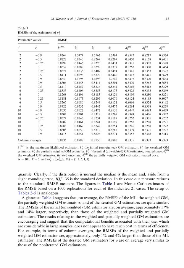
quantile. Clearly, if the distribution is normal the median is the mean and, aside from aslight rounding error, IQ=1:35 is the standard deviation. In this case our measure reducesto the standard RMSE measure. The figures in Table 1 are Monte Carlo estimates ofthe RMSE based on a 1000 replications for each of the indicated 21 cases. The setup ofTables 2–5 is analogous.

A glance at Table 1 suggests that, on average, the RMSEs of the ML, the weighted GM,the partially weighted GM estimators, and of the iterated GM estimators are quite similar.The RMSEs of the initial (unweighted) GM estimator are, on average, approximately 17%and 14% larger, respectively, than those of the weighted and partially weighted GMestimators. The results relating to the weighted and partially weighted GM estimators areencouraging and suggest that the computational benefits associated with their use, whichare considerable in large samples, does not appear to have much cost in terms of efficiency.For example, in terms of column averages, the RMSEs of the weighted and partiallyweighted GM estimator are, approximately, only 1% and 4% larger than those of the MLestimator. The RMSEs of the iterated GM estimators for r are on average very similar tothose of the noniterated GM estimators.

ARTICLE IN PRESS

Table 4

RMSEs of the feasible GLS estimators of b1


J r bbML

1~b1 b1 �b1 ~bð1Þ1 bð1Þ1 �b

ð1Þ

1

2 �0.9 0.2577 0.2600 0.2597 0.2600 0.2581 0.2577 0.2603

2 �0.5 0.2872 0.2885 0.2874 0.2875 0.2889 0.2873 0.2876

2 �0.25 0.3257 0.3248 0.3259 0.3255 0.3250 0.3249 0.3259

2 0 0.3546 0.3551 0.3559 0.3572 0.3542 0.3558 0.3569

2 0.25 0.3709 0.3715 0.3703 0.3731 0.3721 0.3709 0.3732

2 0.5 0.4262 0.4232 0.4234 0.4279 0.4243 0.4252 0.4252

2 0.9 1.1412 1.1330 1.1340 1.1365 1.1379 1.1412 1.1382

6 �0.9 0.2776 0.2729 0.2757 0.2596 0.2740 0.2764 0.2740

6 �0.5 0.3094 0.3104 0.3131 0.3101 0.3112 0.3114 0.3102

6 �0.25 0.3271 0.3321 0.3276 0.3278 0.3313 0.3268 0.3260

6 0 0.3545 0.3500 0.3559 0.3521 0.3534 0.3560 0.3522

6 0.25 0.3777 0.3822 0.3823 0.3811 0.3820 0.3820 0.3807

6 0.5 0.4339 0.4371 0.4363 0.4356 0.4371 0.4377 0.4359

6 0.9 1.1199 1.1176 1.1172 1.1241 1.1195 1.1179 1.1193

10 �0.9 0.2672 0.2730 0.2649 0.2689 0.2656 0.2679 0.2663

10 �0.5 0.3057 0.3084 0.3066 0.3090 0.3069 0.3065 0.3082

10 �0.25 0.3267 0.3287 0.3303 0.3278 0.3299 0.3291 0.3278

10 0 0.3611 0.3568 0.3561 0.3549 0.3600 0.3571 0.3584

10 0.25 0.3870 0.3825 0.3833 0.3847 0.3853 0.3837 0.3859

10 0.5 0.4276 0.4291 0.4287 0.4297 0.4293 0.4288 0.4292

10 0.9 1.1499 1.1475 1.1486 1.1490 1.1462 1.1465 1.1474

Column averages 0.4566 0.4564 0.4564 0.4566 0.4568 0.4567 0.4566

bbML

1 is the maximum likelihood estimator; ~b1 the feasible GLS estimator based on initial GM estimators; b1 the

feasible GLS estimator based on weighted GM estimators; �b1 the feasible GLS estimator based on partially

weighted GM estimators; ~bð1Þ1 the feasible GLS estimator based on initial GM estimators, iterated once; bð1Þ1 the

feasible GLS estimator based on weighted GM estimators, iterated once; and �bð1Þ

1 the feasible GLS estimator

based on partially weighted GM estimators, iterated once.

N ¼ 100, T ¼ 5, and (s2m;s2n ; s

21;b1;b2) ¼ (1,1,6,1,1).

M. Kapoor et al. / Journal of Econometrics 140 (2007) 97–130116

The similarity of the RMSEs of the weighted and partially weighted GM estimatorssuggests that, at least for the weighting matrices considered in our experiments, thecovariance structure of the weighting variance covariance matrix in (26) is not ‘‘veryimportant’’ in determining the efficiency of the corresponding GM estimator. The variancefactors, however, are important. Results of experiments, which are not reported here,reinforce this conjecture. For example, we also explored the small sample properties of anunweighted GM estimator of r based on all six moments, and found that this estimator ismuch less efficient than any of the other estimators, including the initial unweighted GMestimator based only on the first three moments. Upon reflection the reason for this isevident. The variance factors in the variance covariance weighting matrix in (26) ares4n=ðT � 1Þ and s41, where s21 ¼ s2n þ Ts2m. For T ¼ 5, the values of s4n=ðT � 1Þ and s41corresponding to ðs2m;s

2nÞ ¼ ð1; 1Þ are, respectively, 0:25 and 36, implying a ratio of

0:25=36 ¼ 0:0069. The unweighted GM estimator based on six equations gives equalweight to each of the six equations.

ARTICLE IN PRESS

Table 5

RMSEs of feasible GLS estimators of b2


J r bbML

2~b2 b2 �b2 ~bð1Þ2 bð1Þ2 �b

ð1Þ

2

2 �0.9 0.0112 0.0112 0.0112 0.0113 0.0112 0.0112 0.0111

2 �0.5 0.0129 0.0128 0.0128 0.0129 0.0128 0.0129 0.0129

2 �0.25 0.0137 0.0140 0.0137 0.0138 0.0139 0.0137 0.0138

2 0 0.0151 0.0151 0.0152 0.0152 0.0150 0.0152 0.0152

2 0.25 0.0162 0.0162 0.0162 0.0162 0.0162 0.0162 0.0161

2 0.5 0.0162 0.0163 0.0162 0.0161 0.0164 0.0164 0.0161

2 0.9 0.0154 0.0153 0.0153 0.0154 0.0154 0.0154 0.0154

6 �0.9 0.0122 0.0121 0.0122 0.0121 0.0122 0.0123 0.0122

6 �0.5 0.0133 0.0133 0.0133 0.0134 0.0134 0.0132 0.0132

6 �0.25 0.0142 0.0143 0.0143 0.0143 0.0143 0.0142 0.0142

6 0 0.0151 0.0151 0.0152 0.0153 0.0152 0.0152 0.0152

6 0.25 0.0156 0.0154 0.0156 0.0156 0.0154 0.0156 0.0156

6 0.5 0.0158 0.0161 0.0160 0.0159 0.0160 0.0160 0.0160

6 0.9 0.0163 0.0162 0.0163 0.0162 0.0162 0.0163 0.0162

10 �0.9 0.0121 0.0116 0.0120 0.0120 0.0120 0.0121 0.0121

10 �0.5 0.0132 0.0134 0.0133 0.0132 0.0133 0.0133 0.0134

10 �0.25 0.0142 0.0143 0.0142 0.0142 0.0143 0.0142 0.0141

10 0 0.0154 0.0152 0.0151 0.0153 0.0153 0.0153 0.0153

10 0.25 0.0161 0.0159 0.0159 0.0160 0.0160 0.0161 0.0161

10 0.5 0.0170 0.0168 0.0171 0.0170 0.0169 0.0171 0.0171

10 0.9 0.0171 0.0169 0.0171 0.0170 0.0169 0.0171 0.0170

Column averages 0.0147 0.0146 0.0147 0.0147 0.0147 0.0147 0.0147

bbML

2 is the maximum likelihood estimator; ~b2 the feasible GLS estimator based on initial GM estimators; b2 the

feasible GLS estimator based on weighted GM estimators; �b2 the feasible GLS estimator based on partially

weighted GM estimators; ~bð1Þ2 the feasible GLS estimator based on initial GM estimators, iterated once; bð1Þ2 the

feasible GLS estimator based on weighted GM estimators, iterated once; and �bð1Þ

2 the feasible GLS estimator

based on partially weighted GM estimator, iterated once.

Based on N ¼ 100, T ¼ 5, and ðs2m;s2n ; s

21; b1;b2Þ ¼ ð1; 1; 6; 1; 1Þ.


As remarked, our GM estimators for r are not confined to the interval ð�1; 1Þ. However,in our Monte Carlo study we only observed such outliers in less that 1%. As describedabove, our RMSE measure is based on quantiles, and hence it is not effected by thoseinfrequent outliers.

In Tables 2 and 3 we report RMSEs for the GM estimators ~s2n , s2n , �s

2n and �s

21, ~s

21, s

21, the

corresponding iterated GM estimators, and the ML estimators, s2;MLv and s2;ML

1 ,respectively. The RMSEs for the initial GM estimators are again larger than those forthe weighted and partially weighted GM estimators. In contrast to the GM estimators forr, the iterated GM estimators for s2n and s21 exhibit smaller RMSEs than their noniteratedcounter parts. The RMSEs of the weighted GM estimators s2nand ~s21 are on average 2%and 6% higher than the RMSEs of the ML estimators. The difference between the averageRMSEs of the iterated weighted GM estimators and the RMSEs of the ML estimators isless than 1%. The difference between the average RMSEs of the iterated partially weightedGM estimators and the RMSEs of the ML estimators is less than 2%.


In Tables 4 and 5 we report RMSEs for the feasible GLS estimators ~bi;FGLS, bi;FGLS and�bi;FGLS, i ¼ 1; 2, respectively, and iterated versions thereof. Those tables reveal that theRMSEs of the various feasible GLS estimators and the ML estimators for the regressionparameters b1 and b2, respectively, are very similar. These results and those given for theGM estimators of r, s2v and s21 are encouraging, given the computational simplicity of oursuggested estimators relative to the ML estimator.

6. Future research

Several suggestions for future research come to mind. First, on a theoretical level, itwould be of interest to also consider fixed effects specifications. Furthermore, it would be ofinterest to extend the results of this paper to models containing spatially lagged dependentvariables, as well as to systems of equations. In doing this it would certainly be of interest toconsider higher order spatial lags. Another area of interest would be to extend our results tononlinear models. Secondly, a Monte Carlo study relating to a wider set of experiments, aswell as corresponding estimators, than those considered in this paper would be of interest.

Acknowledgments

Kelejian and Prucha gratefully acknowledge financial support from the National ScienceFoundation through Grant SES-0001780. We would like to thank Badi Baltagi and tworeferees for their helpful comments.

Appendix A

Remark A1. In the following we make repeated use of the properties of the matrices Q0;N

and Q1;N discussed after (8). In particular those matrices are symmetric, idempotent andorthogonal, and

Q0;N þQ1;N ¼ INT ,

trðQ0;NÞ ¼ NðT � 1Þ; trðQ1;NÞ ¼ N,

Q0;NðeT � INÞ ¼ 0; Q1;N ðeT � IN Þ ¼ ðeT � IN Þ. (A.1)

Furthermore, let RN be any N �N matrix, then it is readily seen that

ðIT � RN ÞQ0;N ¼ Q0;NðIT � RN Þ; ðIT � RNÞQ1;N ¼ Q1;NðIT � RN Þ,

trðQ0;NðIT � RN ÞÞ ¼ ðT � 1Þ trðRN Þ; trðQ1;NðIT � RN ÞÞ ¼ trðRN Þ, (A.2)

observing that for any T � T matrix ST we have trðST � RN Þ ¼ trðST Þ trðRT Þ.

Remark A2. In the following we shall make repeated use of the following observations:14

(a)

14

Let RN be a (sequence of) N �N matrices whose row and column sums are boundeduniformly in absolute value, and let S be some k � k matrix (with kX1 fixed). Then therow and column sums of S � RN are bounded uniformly in absolute value.

The observations are readily verified. For some explicit proofs see Kelejian and Prucha (1999).


(b)
If AN and BN are (sequences of) kN � kN matrices (with kX1 fixed), whose row andcolumn sums are bounded uniformly in absolute value, then so are the row and columnsums of ANBN and AN þ BN . If ZN is a (sequence of) kN � p matrices whose elementsare uniformly bounded in absolute value, then so are the elements of ANZN andðkNÞ�1Z0NANZN .
Derivation of the moment conditions in (13): Given the error component specification (5)for eN and utilizing the properties of Q0;N and Q1;N described in Remark A1 it follows that:

Q0;NeN ¼ Q0;NnN ,

Q0;NeN ¼ ðIT �W N ÞQ0;NnN ,

Q1;NeN ¼ ðeT � INÞmN þQ1;NnN ,

Q1;NeN ¼ ðeT �W N ÞmN þ ðIT �W N ÞQ1;NnN . (A.3)

Recall that by Assumption 1, EmNm0N ¼ s2mIN , EnNn0N ¼ s2nINT , and EmNn

0N ¼ 0. Also recall

that for any random vector Z and conformable matrix A we have EðZ0AZÞ ¼ trðAEZZ0Þ.Given this, Remark A1, and (A.3) we have

E½e0NQ0;NeN � ¼ E½n0NQ0;NnN �

¼ s2n trðQ0;NÞ ¼ s2nNðT � 1Þ,

E½e0NQ0;NeN � ¼ E½n0NQ0;N ðIT �W 0NW NÞQ0;NnN �

¼ s2n tr½Q0;NðIT �W 0NW N Þ� ¼ s2nðT � 1Þ trðW 0

NW N Þ,

E½e0NQ0;NeN � ¼ E½n0NQ0;NðIT �W 0N ÞQ0;NnN �

¼ s2n tr½Q0;N ðIT �W 0N Þ� ¼ s2nðT � 1Þ trðW 0

N Þ ¼ 0, ðA:4Þ

and

E½e0NQ1;NeN � ¼ E½m0Nðe0T eT � IN ÞmN � þ E½n0NQ1;NnN �

¼ s2m trðe0T eT � IN Þ þ s2n trðQ1;N Þ

¼ NTs2m þNs2n ¼ Ns21,

E½e0NQ1;NeN � ¼ E½m0Nðe0T eT �W 0

NW N ÞmN � þ E½n0NQ1;NðIT �W 0NW N ÞQ1;NnN �

¼ s2m trðe0T eT �W 0NW N Þ þ s2n tr½Q1;N ðIT �W 0

NW NÞ�

¼ Ts2m trðW 0NW NÞ þ s2n trðW 0

NW N Þ ¼ s21 trðW 0NW N Þ,

E½e0NQ1;NeN � ¼ E½m0N ðe0T eT �W 0

NÞmN � þ E½n0NQ1;NðIT �W 0NÞQ1;NnN �

¼ s2m trðe0T eT �W 0NÞ þ s2n tr½Q1;NðIT �W 0

NÞ�

¼ Ts2m trðW 0N Þ þ s2n trðW 0

NÞ ¼ 0, ðA:5Þ

with s21 ¼ Ts2m þ s2n . The moment equations given in (13) now follow immediately from(A.4) and (A.5).

We now give a sequence of lemmata which are needed for the proof of Theorems 1–3.


Lemma A1. Let ST be some T � T matrix (with T fixed ), and let RN be some N �N matrix

whose row and column sums are bounded uniformly in absolute value. Let eN ¼ ðeT �

INÞmN þ nN where mN and nN satisfy Assumption 1. Consider the quadratic form

jN ¼ N�1e0N ðST � RN ÞeN .

Then EjN ¼ Oð1Þ and varðjNÞ ¼ oð1Þ, and as a consequence

jN � EjN!P0 as N !1.

Proof. Let xN ¼ ðx1;N ; . . . ; xðTþ1ÞN ;N Þ0¼ ðm0N ; n

0NÞ0 so that eN ¼ ½ðeT � INÞ; INT �xN and

jN ¼ N�1x0NCNxN with

CN ¼e0T ST eT e0T ST

ST eT ST

" #� RN . (A.6)

Since the first matrix of the Kronecker product in (A.6) does not depend on N it followsimmediately from the maintained assumption concerning RN and Remark A2 that the rowand column sums (and hence the elements) of CN are bounded uniformly in absolute valueby, say kco1. Next observe that in light of Assumption 1 the ðT þ 1ÞN � 1 vector xN hasmean zero, variance covariance matrix

Ox ¼ ExNx0N ¼

s2mIN 0

0 s2nINT

" #,

and finite fourth moments. In the following let 1okZo1 denote an upper bound for the

variances and fourth moments of the elements of mN and nN , and thus of the elements of

xN . Then jEðjNÞj ¼ jN�1 trðCNOxÞjpN�1ð

PðTþ1ÞNi¼1 jcii;N jvarðxi;NÞpðT þ 1ÞkZkco1, and

thus EjN ¼ Oð1Þ. Using the expression for the variance of quadratic forms given, e.g., inKelejian and Prucha (2001), we have

varðjN Þ ¼1

2N2tr½ðCN þ C0NÞOxðCN þ C0NÞOx� þ

XðTþ1ÞNi¼1

c2ii;N ½Ex4i;N � 3 var2ðxi;N Þ�

( ).

Given Remark A2, it is clear that the row and column sums of the absolute values of the

matrix ðCN þ C0N ÞOxðCN þ C0N ÞOx are bounded uniformly by 4k2ck2

Z. Hence, using the

triangle inequality, we have

varðjN Þp1

2N2fðT þ 1ÞN4k2

ck2Z þ ðT þ 1ÞN4k2

ck2Zg ! 0 as N !1,

which shows that varðjN Þ ¼ oð1Þ. The last claim follows immediately from Chebyshev’sinequality. &

Lemma A2. Let G�N and g�N be identical to GN and gN in (15) except that the expectations

operator is dropped. Suppose Assumptions 1, 2, and 4 hold. Then GN ¼ Oð1Þ, gN ¼ Oð1Þand

G�N � GN!P0 and g�N � gN!

P0 as N !1. (A.7)


Proof. Note from (4) that

uN ¼ ½IT � ðIN � rW N Þ�1�eN ¼ ½IT � PN �eN ,

uN ¼ ðIT �W N ÞuN ¼ ðIT �W NPN ÞeN ,

uN ¼ ðIT �W N ÞuN ¼ ðIT �W 2NPN ÞeN . ðA:8Þ

Define

S0;T ¼1

T � 1IT �

JT

T

� �,

S1;T ¼JT

T.

Then, recalling the definition of Q0;N and Q1;N in (8) it is not difficult to verify that therespective quadratic forms in uN , uN , and uN involved in G�N and g�N are, apart from aconstant, expressible as

j1j;N ¼1

NðT � 1Þ1�ju0NQj;NuN ¼

1

Nu0N ðSj;T � IN ÞuN

¼1

Ne0N ðSj;T � R1;NÞeN ; R1;N ¼ P0NPN ,

j2j;N ¼1


1

Nu0N ðSj;T �W NÞuN

¼1

Ne0N ðSj;T � R2;NÞeN ; R2;N ¼ P0NW NPN ,

j3j;N ¼1


1

Nu0N ðSj;T �W 0

NW N ÞuN

¼1

Ne0N ðSj;T � R3;NÞeN ; R3;N ¼ P0NW 0

NW NPN ,

j4j;N ¼1

NðT � 1Þ1�ju0

NQj;NuN ¼1

Nu0N ðSj;T � ðW

0N Þ

2W N ÞuN

¼1

Ne0N ðSj;T � R4;NÞeN ; R4;N ¼ P0NðW

0NÞ

2W NPN ,

j5j;N ¼1

NðT � 1Þ1�ju0

NQj;NuN ¼1

Nu0N ðSj;T � ðW

0N Þ

2W 2N ÞuN

¼1

Ne0N ðSj;T � R5;NÞeN ; R5;N ¼ P0NðW

0NÞ

2W 2NPN ,

j6j;N ¼1


1

Nu0NðSj;T �W 2

N ÞuN

¼1

Ne0NðSj;T � R6;N ÞeN ; R6;N ¼ P0NW 2

NPN , ðA:9Þ

with j ¼ 0; 1. In light of Assumptions 2 and 4 the row and column sums of W N and PN ,and hence those of the matrices Ri;N (i ¼ 1; . . . ; 6), are bounded uniformly in absolute


value; compare Remark A2. The lemma now follows by applying Lemma A1 to each of thequadratic forms in (A.9) which compose G�N and g�N . &

Lemma A3. Let G�N and g�N be as defined in Lemma A2. Then, given Assumptions 1–4

GN � G�N!P0 and gN � g�N!

P0 as N !1 (A.10)

provided ~bN!Pb as N !1.

Proof. The quadratic forms composing the elements of G�N and g�N have been collected in(A.9) and are seen to be of the form ði ¼ 1; . . . ; 6; j ¼ 1; 2Þ:

jij;N ¼ N�1u0NCij;NuN , (A.11)

where the Cij;N are nonstochastic NT �NT matrices. Since the row and column sumsof the elements of W N are uniformly bounded in absolute value it follows that alsothe row and columns sums of the matrices Cij;N have that property; compareRemark A2. The quadratic forms composing the elements of GN and gN defined in (17)are given by

~jij;N ¼ N�1eu0NCij;NeuN . (A.12)

To proof the lemma we now show that ~jij;N � jij;N!P0 as N !1. ClearlyeuN ¼ yN � X N

~bN ¼ uN � X NDN , (A.13)

where DN ¼~bN � b. Since ~bN is consistent, DN!

P0: Substituting (A.13) into (A.12) yields

~jij;N � jij;N ¼ D0NðN�1X 0NCij;NX NÞDN � 2D0N ðN

�1X 0NCij;NuNÞ. (A.14)

Consider the first term on the right-hand side of (A.14). Since the row and column sumsof Cij;N are bounded uniformly in absolute value and since the elements of X N areuniformly bounded in absolute value it follows—see Remark A2—that all K2 elements ofN�1X 0NCij;NX N are Oð1Þ. Therefore, the first term on the right-hand side of (A.14)converges to zero in probability since DN!

P0.

Now consider the second term on the right-hand side of (A.14). In particular, considerthe vector zN ¼ N�1X 0NCij;NuN . Clearly, the mean of zN is zero and its variance covariancematrix is given by

N�1ðN�1X 0NC0ij;NOu;NCij;NX NÞ, (A.15)

where Ou;N is given by (7) and (11). Given the maintained assumptions the row andcolumn sums of Ou;N are uniformly bounded in absolute value, and therefore so arethose of C0ij;NOu;NCij;N . Observing that the elements of X N are uniformly boundedin absolute value, it follows again from the observations in Remark A2 that all K2

elements of N�1X 0NC0ij;NOu;NCij;NX N are Oð1Þ. This implies that the variance covariancematrix of zN given in (A.15) converges to zero, and hence zN converges to zero inprobability. This establishes that also the second term on the right-hand side of (A.14)converges to zero in probability. Thus ~jij;N � jij;N!

P0 as N !1, which completes the

proof. &

Proof of Theorem 1. Observe that by combining Lemmata A2 and A3 we have

GN � GN!P0 and gN � gN!

P0 as N !1. (A.16)


We are now ready for the final step in the proof of Theorem 1. We first demonstrate theconsistency of ~rN and ~s2n;N defined in (24).15 The existence and measurability of ~rN and~s2n;N are ensured by, for example, Lemma 2 in Jennrich (1969). To establish the consistencyof ~rN and ~s2n;N we show that the conditions of Lemma 3.1 in Potscher and Prucha (1997)are satisfied for the problem at hand. Let y ¼ ðr; s2nÞ and y ¼ ðr;s2nÞ. We first show that thetrue parameter vector y is identifiably unique. The objective function of the nonlinear leastsquares estimator and its corresponding nonstochastic counterpart are given by,respectively,

R0N ðyÞ ¼ ½G

0N ½r; r

2; s2n �0 � g0

N �0½G0

N ½r;r2;s2n �

0 � g0N �,

R0

N ðyÞ ¼ ½G0N ½r;r

2;s2n �0 � g0N �

0½G0N ½r;r

2;s2n �0 � g0N �.

Observe that in light of (15) or (18) we have R0

NðyÞ ¼ 0, i.e., R0

NðyÞ is zero at y ¼ y. Then

R0

NðyÞ � R0

NðyÞ ¼ ½r�r;r2 � r2;s2n � s2n �G

00NG

0N ½r�r;r

2 � r2;s2n � s2n �0

XlminðG00NG

0NÞ½r�r;r

2 � r2;s2n � s2n �½r�r;r2 � r2;s2n � s2n �

0

Xl�k y�yk2

in light of Assumption 5. Hence, for every �40 and any N,

inffy:k y�ykX�g

½R0

N ðyÞ � R0

NðyÞ�X inffy:k y�ykX�g

l�k y�yk2 ¼ l��240,

which proves that y is identifiably unique. Next, let F0N ¼ ½G

0N ;�g0

N � and F0N ¼ ½G

0N ;�g

0N �,

then

R0N ðyÞ ¼ ½r; r

2; s2n ; 1�F00NF 0

N ½r;r2;s2n ; 1�,

R0

N ðyÞ ¼ ½r; r2; s2n ; 1�

0F00NF

0N ½r; r

2; s2n ; 1�.

Hence for r 2 ½�a; a� and s2n 2 ½0; b�

jR0N ðyÞ � R

0

N ðyÞj ¼ j½r; r2; s2n ; 1�½F

00NF0

N � F00NF

0N �½r; r

2;s2n ; 1�j

pkF00NF0

N � F00NF

0Nkk r; r

2; s2n ; 1k2

pkF00NF0

N � F00NF

0Nk½1þ a2 þ a4 þ b2

�.

Given (A.16) we have F 0N � F0

N!P0. Observing that by Lemma A2 the elements of F0

N are

Oð1Þ it follows that kF00NF0

N � F00NF

0Nk!

P0, and consequently that R0

N ðyÞ � R0

N ðyÞconverges to zero uniformly over the (extended) parameter space, that is,

supr2½�a;a�;s2n2½0;b�

jR0N ðyÞ � R

0

N ðyÞj

pkF 00NF 0

N � F00NF

0Nk½1þ a2 þ a4 þ b2

�!P0

15This step is analogous to that taken by Kelejian and Prucha (1999) in their consistency proof. We adopt the

following notation: Let A be some vector or matrix, then kAk ¼ ½trðA0AÞ�1=2. We note that this norm is

submultiplicative, i.e., kABkpkAkkBk.


as N !1: The consistency of ~rN and ~s2n;N now follows directly from Lemma 3.1 in

Potscher and Prucha (1997).Next consider ~s21;N defined by (25). In light of (15) we have

~s21;N � s21 ¼ g11;N � g11;N � ðg

111;N � g111;NÞ ~rN � ðg

112;N � g112;N Þ ~r

2N

� g111;N ð ~rN � rÞ � g112;N ð ~r2N � r2Þ.

Observing again that F0N � F0

N!P0 and that the elements of F0

N are Oð1Þ it follows fromthe just established consistency of ~rN that ~s21;N � s21!

P0 as N !1: &

Proof of Consistency of OLS. The least squares estimator of b based on (3) isðX 0NX NÞ

�1X 0NyN . Under the maintained Assumptions 1–4 the estimator is clearly unbiasedand its variance covariance matrix is given by

ðNTÞ�1½ðNTÞ�1X 0NX N ��1ðNTÞ�1X 0NOu;NX N ½ðNT Þ�1X 0NX N �

�1. (A.17)

By Assumption 3, ðNTÞ�1X 0NX N converges to a finite positive definite matrix. As a specialcase of the discussion surrounding (A.15) it is seen that the K2 elements of ðNTÞ�1X 0NOu;NX N

are Oð1Þ. Therefore, the variance covariance matrix in (A.17) converges to zero as N !1,and the consistency of the least squares estimator follows from Chebyshev’s inequality.

Derivation of Variance Covariance Matrix in (26): Assume for the moment thateN�Nð0;Oe;N Þ. The derivation of XN in (26) is straight forward by using the followingresult (compare, e.g., Amemiya, 1973, Lemma): If AN and BN are nonnegative definitesymmetric matrices, then

covðe0NANeN ; e0NBNeNÞ ¼ 2 trðANOe;NBNOe;NÞ.

As an illustration we compute the (2,1)-element of XN . Recall that eN ¼ ðIT �W NÞeN andOe;N ¼ s2nQ0;N þ s21Q1;N . In light of Remark A1 it is not difficult to see that this elementcan be computed as follows:

N cov1

NðT � 1Þe0NQ0;NeN ;

1


� �¼

2

NðT � 1Þ2tr½ðIT �W 0

NÞQ0;N ðIT �W N ÞOe;NQ0Oe;N �

¼2


NW N ÞQ0;NOe;NQ0Oe;N �

¼2s4n


NW N ÞQ0;N � ¼2s4nðT � 1Þ

trW 0

NW N

N

� �.

The derivation of the remaining elements of XN is analogous. &

Proof of Theorem 2. The existence and measurability of the weighted GM estimators rN ,s2n;N , and s21;N defined by (27) are again ensured by Lemma 2 in Jennrich (1969). Lety ¼ ½r;s2n ;s

21� and let y ¼ ½r;s2n ;s

21�. The objective function of the weighted GM estimator

and its corresponding nonstochastic counterpart are then given by, respectively,

RN ðyÞ ¼ ½GN ½r;r2;s2n ;s21�0 � gN �

0 ~X�1N ½GN ½r;r2; s2n ; s21�0 � gN �,

RN ðyÞ ¼ ½GN ½r;r2;s2n ; s21�0 � gN �

0X�1N ½GN ½r;r2;s2n ;s21�0 � gN �.


We now establish two preliminary results implied by the assumptions. First we showthat lminðG0NX

�1N GN ÞXl� for some l�40: To see this let A ¼ ðaijÞ ¼ ðG0

N Þ0ðG0

NÞ andB ¼ ðbijÞ ¼ ðG1

NÞ0ðG1

N Þ. Then in light of (15)

G0NGN ¼

a11 a12 a13 0

a21 a22 a23 0

a31 a32 a33 0

0 0 0 0

2666437775þ

b11 b12 0 b13

b21 b22 0 b23

0 0 0 0

b31 b32 0 b33

2666437775.

Hence, utilizing Assumption 5,

x0G0NGNx ¼ ½x1;x2;x3�A½x1; x2;x3�0 þ ½x1;x2;x4�B½x1;x2;x4�

0

XlminðAÞ½x1;x2; x3�½x1; x2; x3�0 þ lminðBÞ½x1; x2; x4�½x1;x2;x4�

0

Xl�x0x

for any x ¼ ½x1;x2;x3;x4�0. Thus in light of, e.g., Rao (1973, p. 62)

lminðG0NGN Þ ¼ infx

x0G0NGNx

x0xXl�40.

Next observe that

lminðG0NX�1N GNÞ ¼ inf

x

x0G0NX�1N GNx

x0xXlminðX�1N Þ infx

x0G0NGNx

x0x

¼ lminðX�1N ÞlminðG0NGNÞXl�40,

with l� ¼ l�l�, since lminðX�1N ÞXl�40 by assumption.Second, we show that X�1N ¼ Oð1Þ. For notational convenience let SN ¼ X�1N . To verify

the claim we need to show that sij;N

�� pko1 for some constant k that does not depend onN. Again in light of, e.g., Rao (1973, p. 62),

lminðSNÞ ¼ infx

x0SNx

x0x; lmaxðSN Þ ¼ max

x

x0SNx

x0x.

Hence it follows from the maintained assumptions concerning the smallest and largesteigenvalues of SN ¼ X�1N that

0ol�px0SNx

x0xpl��o1.

Taking x to be the vector that has a one in the ith and jth positions and zeros elsewherewe have

0psii;Npl��o1; i ¼ j;

0pðsii;N þ sjj;N þ 2sij;N Þ=2pl��o1; iaj:

From this it is readily seen that jsij;N jpl�� for all i; j, which proves the claim.Analogous as in the proof of Theorem 1 observe that RN ðyÞ is zero at y ¼ y, and hence

RNðyÞ � RNðyÞ

¼ ½r�r;r2 � r2;s2n � s2n ; s21 � s21�G

0NX�1N GN ½r�r;r2 � r2;s2n � s2n ; s

21 � s21�

0.


Next, let FN ¼ ½GN ;�gN � and FN ¼ ½GN ;�gN �, then

RN ðyÞ ¼ ½r; r2;s2n ;s21; 1�F

0N~X�1N F N ½r;r2;s2n ;s

21; 1�,

RN ðyÞ ¼ ½r; r2;s2n ;s21; 1�

0F0NX�1N FN ½r; r2; s2n ;s

21; 1�.

The remainder of the proof of Theorem 2 is now analogous to that of Theorem 1. &

Proof of Theorem 3. Let l� ¼ minfðT � 1Þs�4n ;s�41 g and l�� ¼ maxfðT � 1Þs�4n ;s�41 g. Then0ol�plminðU �1N ÞplmaxðU �1N Þpl��o1. The proof of Theorem 3 is now analogous to thatof Theorem 2 with XN and ~XN replaced by UN and ~UN , respectively. &

Proof of Theorem 4. Part (a): We prove this part by verifying the conditions of the centrallimit theorem given in Potscher and Prucha (2001) as Theorem 30.16 First observe that(30)–(32) imply

ðNTÞ1=2½bbGLS;N � b�

¼ ½ðNTÞ�1X 0NO�1u;NX N �

�1ðNTÞ�1=2X 0NO�1u;NuN

¼ ½ðNTÞ�1X �NðrÞ0O�1e;NX �NðrÞ�

�1ðNTÞ�1=2X �N ðrÞ0O�1e;NeN . ðA:18Þ

Consider the first factor in the last expression in (A.18). Recalling that O�1e;N ¼ s�2n Q0;N þ

s�21 Q1;N it follows from Assumption 3 and the discussion thereafter that

limN!1ðNT Þ�1X �NðrÞ

0O�1e;NX �NðrÞ ¼ s�2n M0xx þ s�21 M1

xx, (A.19)

which is a finite nonsingular matrix. Now consider the second factor in the last expressionin (A.18). The results in (A.3) imply

ðNTÞ�1=2X �N ðrÞ0O�1e;NeN

¼ ðNTÞ�1=2X �N ðrÞ0½s�2n Q0;N þ s�21 Q1;N �eN

¼ ðNTÞ�1=2Z01;NmN þ ðNTÞ�1=2Z02;NnN , ðA:20Þ

where

Z01;N ¼ X �NðrÞ0ðs�21 ðeT � IN ÞÞ and Z02;N ¼ X �N ðrÞ

0ðs�2n Q0;N þ s�21 Q1;NÞ.

Given Assumptions 3 and 4 it follows from the observations in Remark A2 that theelements of Z1;N and Z2;N are uniformly bounded in absolute value, and furthermore

limN!1ðNT Þ�1Z01;NZ1;N ¼ lim

N!1ðNTÞ�1Ts�41 X �NðrÞ

0Q1;NX �N ðrÞ

¼ Ts�41 M1xx,

limN!1ðNT Þ�1Z02;NZ2;N ¼ lim

N!1ðNTÞ�1½X �NðrÞ

0ðs�4n Q0;N þ s�41 Q1;N ÞX

�NðrÞ�

¼ s�4n M0xx þ s�41 M1

xx. ðA:21Þ

16An inspection of the proof of that theorem shows that the theorem also holds if the innovations are allowed to

form a triangular array and the sample index n is replaced by rn.


The matrices on the right-hand side of (A.21) are finite. Given Assumption 1 it now followsfrom Theorem 30 in Potscher and Prucha (2001) that

ðNT Þ�1=2Z01;NmN!D

Nf0;Ts2ms�41 M1

xxg,

ðNT Þ�1=2Z02;NnN!D

Nf0;s2n ½s�4n M0

xx þ s�41 M1xx�g. ðA:22Þ

Since s21 ¼ s2n þ Ts2m and, by Assumption 1, the two processes {mi;Ng and {nit;Ng areindependent, it follows furthermore from (A.20) and (A.22) that

ðNT Þ�1=2X �NðrÞ0O�1e;NeN!

DNð0; s�2n M0

xx þ s�21 M1xxÞ (A.23)

as N !1. Part (a) of Theorem 4 follows from the results in (A.18), (A.19) and (A.23).Part (b): To prove this part it suffices to show that17

D1;N ¼ ðNTÞ�1X �N ð �rN Þ0 �O�1

e;NX �Nð �rN Þ � ðNTÞ�1X �NðrÞ0O�1e;NX �NðrÞ!

P0, (A.24)

and

D2;N ¼ ðNTÞ�1=2X �N ð �rNÞ0 �O�1

e;Nu�Nð �rN Þ � ðNTÞ�1=2X �NðrÞ0O�1e;Nu�NðrÞ!

P0, (A.25)

where �O�1

e;N ¼ O�1e;Nð �s2n;N ; �s

21;N Þ and u�N ð �rNÞ ¼ ðIN � �rNW NÞuN .

We first demonstrate (A.24). To this effect first substitute the expression for X �Nð �rN Þ

given in (31) into (A.24). Then, observing that in light of (9) and Remark A1

O�1e;N ½IT � ðIN � rW NÞ� ¼ ½IT � ðIN � rW NÞ�O�1e;N ,

�O�1

e;N ½IT � ðIN � �rNW N Þ� ¼ ½IT � ðIN � �rNW NÞ� �O�1

e;N , ðA:26Þ

it is readily seen that

D1;N ¼ ½ �rN � r� �s�2n;N ðNT Þ�1X 0NA1;NX N þ ½ �rN � r� �s�21;NðNTÞ�1X 0NA2;NX N

þ ½ �r2N � r2� �s�2n;N ðNT Þ�1X 0NA3;NX N þ ½ �r2N � r2� �s�21;N ðNT Þ�1X 0NA4:NX N

þ ½ �s�2n;N � s�2n �ðNTÞ�1X 0NA5;NX N þ ½ �s�21;N � s�21 �ðNTÞ�1X 0NA6;NX N , ðA:27Þ

where

A1;N ¼ ½IT � ðW0N þW NÞ�Q0;N ,

A2;N ¼ ½IT � ðW0N þW NÞ�Q1;N ,

A3;N ¼ ½IT � ðW0NW N Þ�Q0;N �,

A4;N ¼ ½IT � ðW0NW N Þ�Q1;N ,

A5;N ¼ ½IT � ðIN � rW 0N ÞðIN � rW NÞ�Q0;N ,

A6;N ¼ ½IT � ðIN � rW 0N ÞðIN � rW NÞ�Q1;N . ðA:28Þ

In light of Remark A2 and Assumptions 3 and 4, the elements of the six K � K matricesðNTÞ�1X 0NAi;NX N , i ¼ 1; . . . ; 6, are seen to be uniformly bounded in absolute value. Since�rN ; �s

2n;N , and �s21;N are consistent estimators it follows that D1;N!

P0 as N !1.

17See, e.g., Schmidt (1976, p. 71).


We next demonstrate (A.25). Using similar manipulations we have

D2;N ¼ ½ �rN � r� �s�2n;NðNTÞ�1=2X 0NA1;NuN þ ½ �rN � r� �s�21;N ðNTÞ�1=2X 0NA2;NuN

þ ½ �r2N � r2� �s�2n;NðNTÞ�1=2X 0NA3;NuN þ ½ �r2N � r2� �s�21;NðNTÞ�1=2X 0NA4:NuN

þ ½ �s�2n;N � s�2n �ðNTÞ�1=2X 0NA5;NuN þ ½ �s�21;N � s�21 �ðNTÞ�1=2X 0NA6;NuN . ðA:29Þ

Since X N and Ai;N are nonstochastic matrices the expected values of the K � 1 vectorsðNT Þ�1=2X 0NAi;NuN are zero and their variance covariance matrices are given by(i ¼ 1; . . . ; 6)

ðNTÞ�1X 0NAi;NOu;NA0i;NX N ,

where Ou;N is defined via (7) and (11). Given Assumptions 3 and 4 and Remarks A1 and A2the row and column sums of Ou;N , and furthermore those of Ai;NOu;NA0i;N , are uniformlybounded in absolute value. Hence, the elements of the K � K matrices ðNT Þ�1X 0NAi;NOu;NA0i;NX N are uniformly bounded in absolute value. Therefore ðNT Þ�1=2X 0NAi;NuN ¼

OPð1Þ and thus D2;N!P0 as N !1, since �rN , �s

2n;N , and �s21;N are consistent estimators.

Part (c): This part follows immediately from (A.19) and (A.24). &

References

Amemiya, T., 1971. The estimation of the variances in a variance-component model. International Economic

Review 12, 1–13.

Amemiya, T., 1985. Advanced Econometrics. Harvard University Press, Cambridge, MA.

Anselin, L., 1988. Spatial Econometrics: Methods and Models. Kluwer Academic Publishers, Boston.

Audretsch, D.B., Feldmann, M.P., 1996. R&D spillovers and the geography of innovation and production.

American Economic Review 86, 630–640.

Balestra, P., Nerlove, M., 1966. Pooling cross section and time series data in the estimation of a dynamic model:

the demand for natural gas. Econometrica 34, 585–612.

Baltagi, B.H., 1980. On seemingly unrelated regressions with error components. Econometrica 48, 1547–1551.

Baltagi, B.H., 1981. Simultaneous equations with error components. Journal of Econometrics 17, 189–200.

Baltagi, B.H., 2001. Econometric Analysis of Panel Data. Wiley, New York.

Baltagi, B.H., Li, D., 2001a. Double length artificial regressions for testing spatial dependence. Econometric

Reviews 20, 31–40.

Baltagi, B.H., Li, D., 2001b. LM test for functional form and spatial error correlation. International Regional

Science Review 24, 194–225.

Baltagi, B.H., Li, D., 2004. Prediction in the panel data model with spatial correlation. In: Anselin, L., Florax,

R.J.G.M., Rey, S.J. (Eds.), Advances in Spatial Econometrics: Methodology, Tools and Applications.

Springer, Berlin, pp. 283–295.

Baltagi, B.H., Song, S.H., Koh, W., 2003. Testing panel data regression models with spatial error correlation.

Journal of Econometrics 117, 123–150.

Bernat Jr., G., 1996. Does manufacturing matter? A spatial econometric view of Kaldor’s laws. Journal of

Regional Science 36, 463–477.

Besley, T., Case, A., 1995. Incumbent behavior: vote-seeking, tax-setting, and yardstick competition. American

Economic Review 85, 25–45.

Bollinger, C., Ihlanfeldt, K., 1997. The impact of rapid rail transit on economic development: the case of Atlanta’s

Marta. Journal of Urban Economics 42, 179–204.

Buettner, T., 1999. The effect of unemployment, aggregate wages, and spatial contiguity on local wages: an

investigation with German district level data. Papers in Regional Science 78, 47–67.

Case, A., 1991. Spatial patterns in household demand. Econometrica 59, 953–966.


Case, A., Hines Jr., J., Rosen, H., 1993. Budget spillovers and fiscal policy independence: evidence from the States.

Journal of Public Economics 52, 285–307.

Cliff, A., Ord, J., 1973. Spatial Autocorrelation. Pion, London.

Cliff, A., Ord, J., 1981. Spatial Processes, Models and Applications. Pion, London.

Conley, T., 1999. GMM estimation with cross sectional dependence. Journal of Econometrics 92, 1–45.

Cressie, N.A.C., 1993. Statistics of Spatial Data. Wiley, New York.

Das, D., Kelejian, H.H., Prucha, I.R., 2003. Small sample properties of estimators of spatial autoregressive

models with autoregressive disturbances. Papers in Regional Science 82, 1–26.

Dowd, M.R., LeSage, J.P., 1997. Analysis of spatial contiguity influences on state price level formation.

International Journal of Forecasting 13, 245–253.

Gallant, A.R., White, H., 1988. A Unified Theory of Estimation and Inference in Nonlinear Dynamic Models.

Basil Blackwell, New York.

Holtz-Eakin, D., 1994. Public sector capital and the productivity puzzle. Review of Economics and Statistics 76,

12–21.

Horn, R., Johnson, C., 1985. Matrix Analysis. Cambridge University Press, Cambridge.

Hsiao, C., 2003. Analysis for Panel Data. Cambridge University Press, Cambridge.

Jennrich, R., 1969. Asymptotic properties of non-linear least squares estimators. The Annals of Mathematical

Statistics 40, 633–643.

Kelejian, H.H., Prucha, I.R., 1997. Estimation of spatial regression models with autoregressive errors

by two-stage least squares procedures: a serious problem. International Regional Science Review 20,

103–111.

Kelejian, H.H., Prucha, I.R., 1998. A generalized spatial two-stage least squares procedure for estimating a spatial

autoregressive model with autoregressive disturbances. Journal of Real Estate Finance and Economics 17,

99–121.

Kelejian, H.H., Prucha, I.R., 1999. A generalized moments estimator for the autoregressive parameter in a spatial

model. International Economic Review 40, 509–533.

Kelejian, H.H., Prucha, I.R., 2001. On the asymptotic distribution of the Moran I test statistic with applications.


Kelejian, H.H., Prucha, I.R., 2004. Estimation of systems of spatially interrelated cross sectional equations.


Kelejian, H.H., Robinson, D., 1997. Infrastructure productivity estimation and its underlying econometric

specifications. Papers in Regional Science 76, 115–131.

Kelejian, H.H., Robinson, D., 2000. Returns to investment in navigation infrastructure: an equilibrium approach.

Annals of Regional Science 34, 83–108.

Kelejian, H.H., Prucha, I.R., Yuzefovich, E., 2004, Instrumental variable estimation of a spatial autorgressive

model with autoregressive disturbances: large and small sample results. In: LeSage, J., Pace, R.K. (Eds.),

Spatial and Spatiotemporal Econometrics, Advances in Econometrics, Vol. 18. Elsevier, New York,

pp. 163–198.

Lee, L.-F., 2001a. Generalized method of moments estimation of spatial autoregressive processes. Mimeo,

Department of Economics, Ohio State University.

Lee, L.-F., 2001b. GMM and 2SLS estimation of mixed regressive, spatial autoregressive models. Mimeo,

Department of Economics, Ohio State University.

Lee, L.F., 2002. Consistency and efficiency of least squares estimation for mixed regressive, spatial autoregressive

models. Econometric Theory 18, 252–277.

Lee, L.F., 2003. Best spatial two-stage least squares estimators for a spatial autoregressive model with

autoregressive disturbances. Econometric Reviews 22, 307–335.

Lee, L.F., 2004. Asymptotic distributions of quasi-maximum likelihood estimators for spatial autoregressive

models. Econometrica 72, 1899–1925.

LeSage, J.P., 1997. Bayesian estimation of spatial autoregressive models. International Regional Science Review

20, 113–129.

LeSage, J.P., 1999. A spatial econometric analysis of China’s economic growth. Journal of Geographic

Information Sciences 5, 143–153.

LeSage, J.P., 2000. Bayesian estimation of limited dependent variable spatial autoregressive models. Geographic

Analysis 32, 19–35.

Nerlove, M., 1971. A note on error component models. Econometrica 39, 383–396.

Pace, R., Barry, R., 1997. Sparse spatial autoregressions. Statistics and Probability Letters 33, 291–297.


Pinkse, J., Slade, M.E., 1998. Contracting in space: an application of spatial statistics to discrete-choice models.


Pinkse, J., Slade, M.E., Brett, C., 2002. Spatial price competition: a semiparametric approach. Econometrica 70,

1111–1153.

Potscher, B.M., Prucha, I.R., 1997. Dynamic Nonlinear Econometric Models, Asymptotic Theory. Springer, New

York.

Potscher, B.M., Prucha, I.R., 2001. Basic elements of asymptotic theory. In: Baltagi, B.H. (Ed.), A Companion to

Theoretical Econometrics. Blackwell, Oxford, pp. 201–229.

Prucha, I.R., 1984. On the asymptotic efficiency of feasible Aitken estimators for seemingly unrelated regression

models with error components. Econometrica 52, 203–207.

Prucha, I.R., 1985. Maximum likelihood and instrumental variable estimation in simultaneous equation systems

with error components. International Economic Review 26, 491–506.

Rao, C.R., 1973. Linear Statistical Inference and Its Applications. Wiley, New York.

Rey, S.J., Boarnet, M.G., 2004. A taxonomy of spatial econometric models for simultaneous equation systems. In:

Anselin, L., Florax, R.J.G.M., Rey, S.J. (Eds.), Advances in Spatial Econometrics: Methodology Tools and

Applications. Springer, Berlin, pp. 99–119.

Schmidt, P., 1976. Econometrics. Marcel Dekker, New York.

Shroder, M., 1995. Games the states don’t play: welfare benefits and the theory of fiscal federalism. Review of

Economics and Statistics 77, 183–191.

Vigil, R., 1998. Interactions among municipalities in the provision of police services: a spatial econometric

approach, Ph.D. Thesis, University of Maryland.

Wallace, T.D., Hussain, A., 1969. The use of error component models in combining cross section with time series

data. Econometrica 37, 55–72.

Panel data models with spatially correlated error...

Documents

Transcript of Panel data models with spatially correlated error...