Pan Pan Cheng Essay - University of Waterloo
27
S TUDY OF D ECONVOLUTIONAL S ENTENCE R ECONSTRUCTION APREPRINT Pan Pan Cheng Department of Computer Science University of Waterloo Waterloo, ON N2L 3G1 [email protected] May 17, 2019 ABSTRACT Finding an effective latent sentence representation is often a required step in most of the natural language processing (NLP) research. Most of the time, people are using recurrent neural networks to extract this latent representation with additional techniques like attention mechanism and teacher forcing. However, such techniques might weaken the amount of information carried inside the latent representation because the decoding process is not relying on the latent representation solely, but more on some external signals. In this essay, we are going to explore how we make use of deconvolution networks for sentence reconstruction. This can be potentially extended to solve other NLP tasks such as machine translation and sentiment analysis. From our sentence reconstruction experiment, the deconvolutional method outperforms a standard RNN method on short sentences. Keywords Encoder-Decoder · Deconvolution · Sum Product Networks (SPNs) 1 Introduction Learning an efficient representation of a sentence or a paragraph is often required in many natural language processing applications such as machine translation and sentiment analysis. A popular way to learn an effective representation from a sentence is to use the Encoder - Decoder framework. In a typical setup of the Encoder - Decoder framework, an input sentence is first converted into either a one-hot encoding vector or a matrix representation of word embeddings. The matrix representation is most often of dimensionality number of words × word embedding size. The word embedding can be either learned from the data or imported from some pre-trained libraries like Word2vec, GloVe, etc. An encoder is then applied to the given one-hot encoding vector or word embedding matrix for a low-dimensional form, and followed by a decoder to reconstruct the input sequence from the latent representation. The Encoder - Decoder framework is mostly used in neural machine translation (NMT). A popular choice of the architecture is to use recurrent neural network (RNN) based methods for both encoders and decoders. To be specific, researchers use a bi-directional RNN to encode an input sequence of variable-length to a latent representation, and then decode it to the target output sequence using another RNN. Typically researchers choose long short term memory networks (LSTM) or gated recurrent networks (GRU) as the recurrent layer. More often those recurrent layers are equipped with techniques such as soft-attention mechanism and teacher-forcing training. However, those techniques might reduce the level of information that the latent representation can carry. This is because the decoding process now requires additional resources or guidance in order to reconstruct the sentence. This might contradict the objective to look for an effective vector representation that carries sufficient information for the sentence recovery process. Researchers more often focus on ways to use convolutions for the encoding process than decoding ([4], [5], [8], [9]). Sometimes they might propose a very deep convolution encoding layer to capture information such as [17] using a 29-layer convolution network for text classification. But from our study, with an appropriate decoding process, the encoding could be a lot smaller to achieve satisfactory results for natural language processing tasks. Today we are going to examine and explore the deconvolution architecture proposed by [20] with some modification to fit our target data set.
Transcript of Pan Pan Cheng Essay - University of Waterloo
STUDY OF DECONVOLUTIONAL SENTENCE RECONSTRUCTION
A PREPRINT
Pan Pan ChengDepartment of Computer Science
University of WaterlooWaterloo, ON N2L [email protected]
May 17, 2019
ABSTRACT
Finding an effective latent sentence representation is often a required step in most of the naturallanguage processing (NLP) research. Most of the time, people are using recurrent neural networksto extract this latent representation with additional techniques like attention mechanism and teacherforcing. However, such techniques might weaken the amount of information carried inside the latentrepresentation because the decoding process is not relying on the latent representation solely, but moreon some external signals. In this essay, we are going to explore how we make use of deconvolutionnetworks for sentence reconstruction. This can be potentially extended to solve other NLP tasks suchas machine translation and sentiment analysis. From our sentence reconstruction experiment, thedeconvolutional method outperforms a standard RNN method on short sentences.
Keywords Encoder-Decoder · Deconvolution · Sum Product Networks (SPNs)
1 Introduction
Learning an efficient representation of a sentence or a paragraph is often required in many natural language processingapplications such as machine translation and sentiment analysis. A popular way to learn an effective representation froma sentence is to use the Encoder - Decoder framework. In a typical setup of the Encoder - Decoder framework, an inputsentence is first converted into either a one-hot encoding vector or a matrix representation of word embeddings. Thematrix representation is most often of dimensionality number of words × word embedding size. The word embeddingcan be either learned from the data or imported from some pre-trained libraries like Word2vec, GloVe, etc. An encoder isthen applied to the given one-hot encoding vector or word embedding matrix for a low-dimensional form, and followedby a decoder to reconstruct the input sequence from the latent representation.
The Encoder - Decoder framework is mostly used in neural machine translation (NMT). A popular choice of thearchitecture is to use recurrent neural network (RNN) based methods for both encoders and decoders. To be specific,researchers use a bi-directional RNN to encode an input sequence of variable-length to a latent representation, andthen decode it to the target output sequence using another RNN. Typically researchers choose long short term memorynetworks (LSTM) or gated recurrent networks (GRU) as the recurrent layer. More often those recurrent layers areequipped with techniques such as soft-attention mechanism and teacher-forcing training. However, those techniquesmight reduce the level of information that the latent representation can carry. This is because the decoding process nowrequires additional resources or guidance in order to reconstruct the sentence. This might contradict the objective tolook for an effective vector representation that carries sufficient information for the sentence recovery process.
Researchers more often focus on ways to use convolutions for the encoding process than decoding ([4], [5], [8], [9]).Sometimes they might propose a very deep convolution encoding layer to capture information such as [17] using a29-layer convolution network for text classification. But from our study, with an appropriate decoding process, theencoding could be a lot smaller to achieve satisfactory results for natural language processing tasks. Today we are goingto examine and explore the deconvolution architecture proposed by [20] with some modification to fit our target data set.
A PREPRINT - MAY 17, 2019
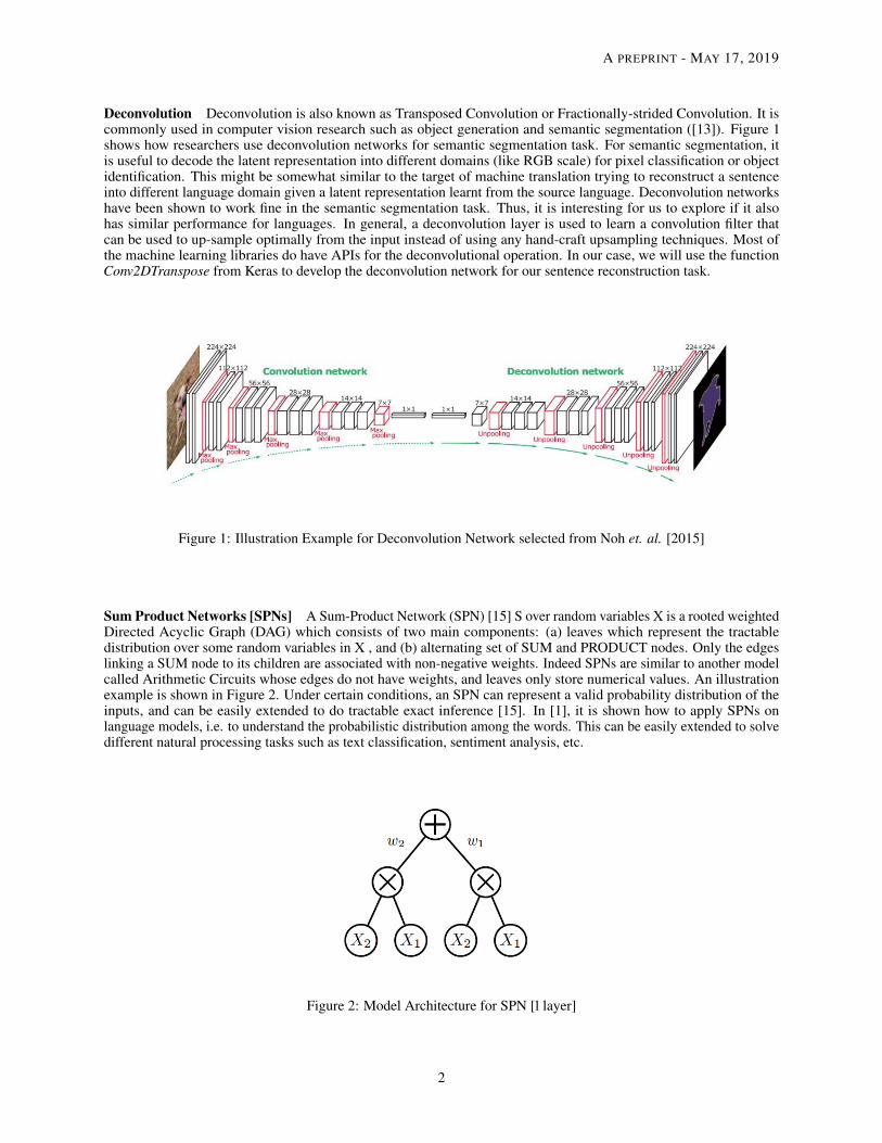
Deconvolution Deconvolution is also known as Transposed Convolution or Fractionally-strided Convolution. It iscommonly used in computer vision research such as object generation and semantic segmentation ([13]). Figure 1shows how researchers use deconvolution networks for semantic segmentation task. For semantic segmentation, itis useful to decode the latent representation into different domains (like RGB scale) for pixel classification or objectidentification. This might be somewhat similar to the target of machine translation trying to reconstruct a sentenceinto different language domain given a latent representation learnt from the source language. Deconvolution networkshave been shown to work fine in the semantic segmentation task. Thus, it is interesting for us to explore if it alsohas similar performance for languages. In general, a deconvolution layer is used to learn a convolution filter thatcan be used to up-sample optimally from the input instead of using any hand-craft upsampling techniques. Most ofthe machine learning libraries do have APIs for the deconvolutional operation. In our case, we will use the functionConv2DTranspose from Keras to develop the deconvolution network for our sentence reconstruction task.
Figure 1: Illustration Example for Deconvolution Network selected from Noh et. al. [2015]
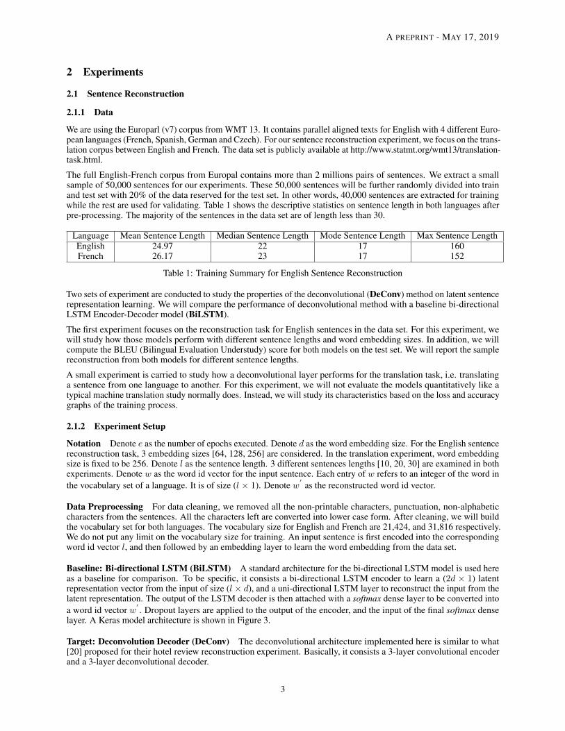
Sum Product Networks [SPNs] A Sum-Product Network (SPN) [15] S over random variables X is a rooted weightedDirected Acyclic Graph (DAG) which consists of two main components: (a) leaves which represent the tractabledistribution over some random variables in X , and (b) alternating set of SUM and PRODUCT nodes. Only the edgeslinking a SUM node to its children are associated with non-negative weights. Indeed SPNs are similar to another modelcalled Arithmetic Circuits whose edges do not have weights, and leaves only store numerical values. An illustrationexample is shown in Figure 2. Under certain conditions, an SPN can represent a valid probability distribution of theinputs, and can be easily extended to do tractable exact inference [15]. In [1], it is shown how to apply SPNs onlanguage models, i.e. to understand the probabilistic distribution among the words. This can be easily extended to solvedifferent natural processing tasks such as text classification, sentiment analysis, etc.
Figure 2: Model Architecture for SPN [l layer]
2
A PREPRINT - MAY 17, 2019
2 Experiments
2.1 Sentence Reconstruction
2.1.1 Data
We are using the Europarl (v7) corpus from WMT 13. It contains parallel aligned texts for English with 4 different Euro-pean languages (French, Spanish, German and Czech). For our sentence reconstruction experiment, we focus on the trans-lation corpus between English and French. The data set is publicly available at http://www.statmt.org/wmt13/translation-task.html.
The full English-French corpus from Europal contains more than 2 millions pairs of sentences. We extract a smallsample of 50,000 sentences for our experiments. These 50,000 sentences will be further randomly divided into trainand test set with 20% of the data reserved for the test set. In other words, 40,000 sentences are extracted for trainingwhile the rest are used for validating. Table 1 shows the descriptive statistics on sentence length in both languages afterpre-processing. The majority of the sentences in the data set are of length less than 30.
Language Mean Sentence Length Median Sentence Length Mode Sentence Length Max Sentence LengthEnglish 24.97 22 17 160French 26.17 23 17 152
Table 1: Training Summary for English Sentence Reconstruction
Two sets of experiment are conducted to study the properties of the deconvolutional (DeConv) method on latent sentencerepresentation learning. We will compare the performance of deconvolutional method with a baseline bi-directionalLSTM Encoder-Decoder model (BiLSTM).
The first experiment focuses on the reconstruction task for English sentences in the data set. For this experiment, wewill study how those models perform with different sentence lengths and word embedding sizes. In addition, we willcompute the BLEU (Bilingual Evaluation Understudy) score for both models on the test set. We will report the samplereconstruction from both models for different sentence lengths.
A small experiment is carried to study how a deconvolutional layer performs for the translation task, i.e. translatinga sentence from one language to another. For this experiment, we will not evaluate the models quantitatively like atypical machine translation study normally does. Instead, we will study its characteristics based on the loss and accuracygraphs of the training process.
2.1.2 Experiment Setup
Notation Denote e as the number of epochs executed. Denote d as the word embedding size. For the English sentencereconstruction task, 3 embedding sizes [64, 128, 256] are considered. In the translation experiment, word embeddingsize is fixed to be 256. Denote l as the sentence length. 3 different sentences lengths [10, 20, 30] are examined in bothexperiments. Denote w as the word id vector for the input sentence. Each entry of w refers to an integer of the word inthe vocabulary set of a language. It is of size (l × 1). Denote w
′as the reconstructed word id vector.
Data Preprocessing For data cleaning, we removed all the non-printable characters, punctuation, non-alphabeticcharacters from the sentences. All the characters left are converted into lower case form. After cleaning, we will buildthe vocabulary set for both languages. The vocabulary size for English and French are 21,424, and 31,816 respectively.We do not put any limit on the vocabulary size for training. An input sentence is first encoded into the correspondingword id vector l, and then followed by an embedding layer to learn the word embedding from the data set.
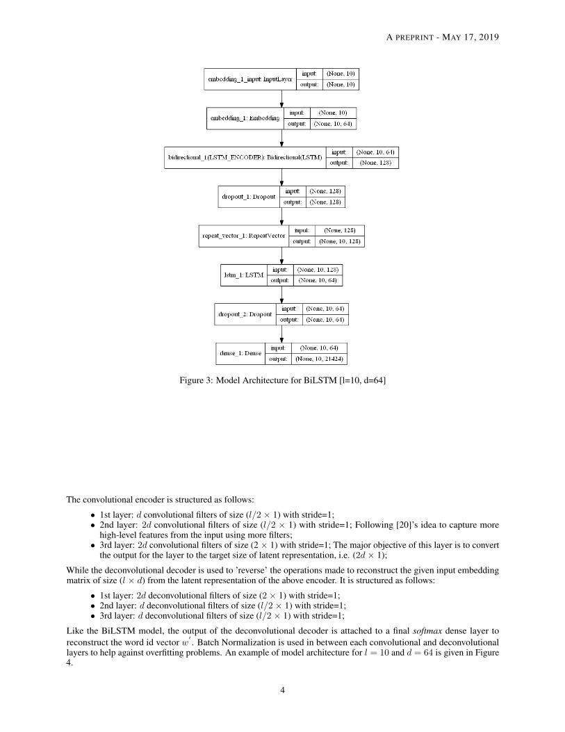
Baseline: Bi-directional LSTM (BiLSTM) A standard architecture for the bi-directional LSTM model is used hereas a baseline for comparison. To be specific, it consists a bi-directional LSTM encoder to learn a (2d × 1) latentrepresentation vector from the input of size (l × d), and a uni-directional LSTM layer to reconstruct the input from thelatent representation. The output of the LSTM decoder is then attached with a softmax dense layer to be converted intoa word id vector w
′. Dropout layers are applied to the output of the encoder, and the input of the final softmax dense
layer. A Keras model architecture is shown in Figure 3.
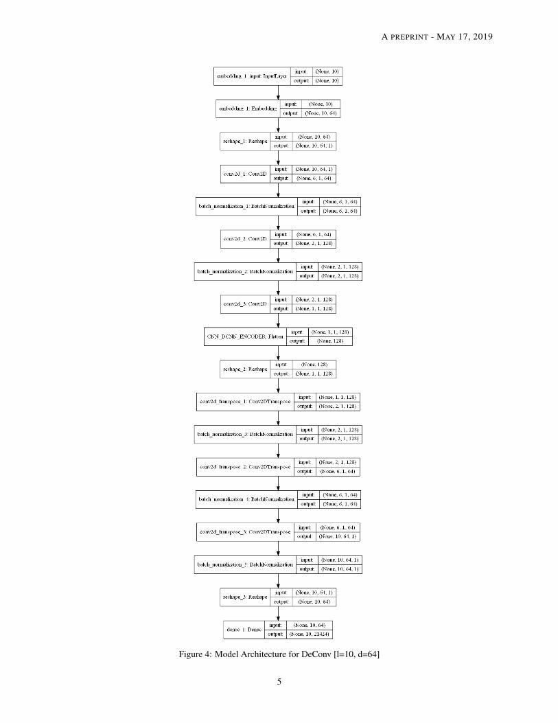
Target: Deconvolution Decoder (DeConv) The deconvolutional architecture implemented here is similar to what[20] proposed for their hotel review reconstruction experiment. Basically, it consists a 3-layer convolutional encoderand a 3-layer deconvolutional decoder.
3
A PREPRINT - MAY 17, 2019
Figure 3: Model Architecture for BiLSTM [l=10, d=64]
The convolutional encoder is structured as follows:
• 1st layer: d convolutional filters of size (l/2 × 1) with stride=1;• 2nd layer: 2d convolutional filters of size (l/2 × 1) with stride=1; Following [20]’s idea to capture more
high-level features from the input using more filters;• 3rd layer: 2d convolutional filters of size (2 × 1) with stride=1; The major objective of this layer is to convert
the output for the layer to the target size of latent representation, i.e. (2d × 1);
While the deconvolutional decoder is used to ’reverse’ the operations made to reconstruct the given input embeddingmatrix of size (l × d) from the latent representation of the above encoder. It is structured as follows:
• 1st layer: 2d deconvolutional filters of size (2 × 1) with stride=1;• 2nd layer: d deconvolutional filters of size (l/2 × 1) with stride=1;• 3rd layer: d deconvolutional filters of size (l/2 × 1) with stride=1;
Like the BiLSTM model, the output of the deconvolutional decoder is attached to a final softmax dense layer toreconstruct the word id vector w
′. Batch Normalization is used in between each convolutional and deconvolutional
layers to help against overfitting problems. An example of model architecture for l = 10 and d = 64 is given in Figure4.
4
A PREPRINT - MAY 17, 2019
Figure 4: Model Architecture for DeConv [l=10, d=64]
5
A PREPRINT - MAY 17, 2019
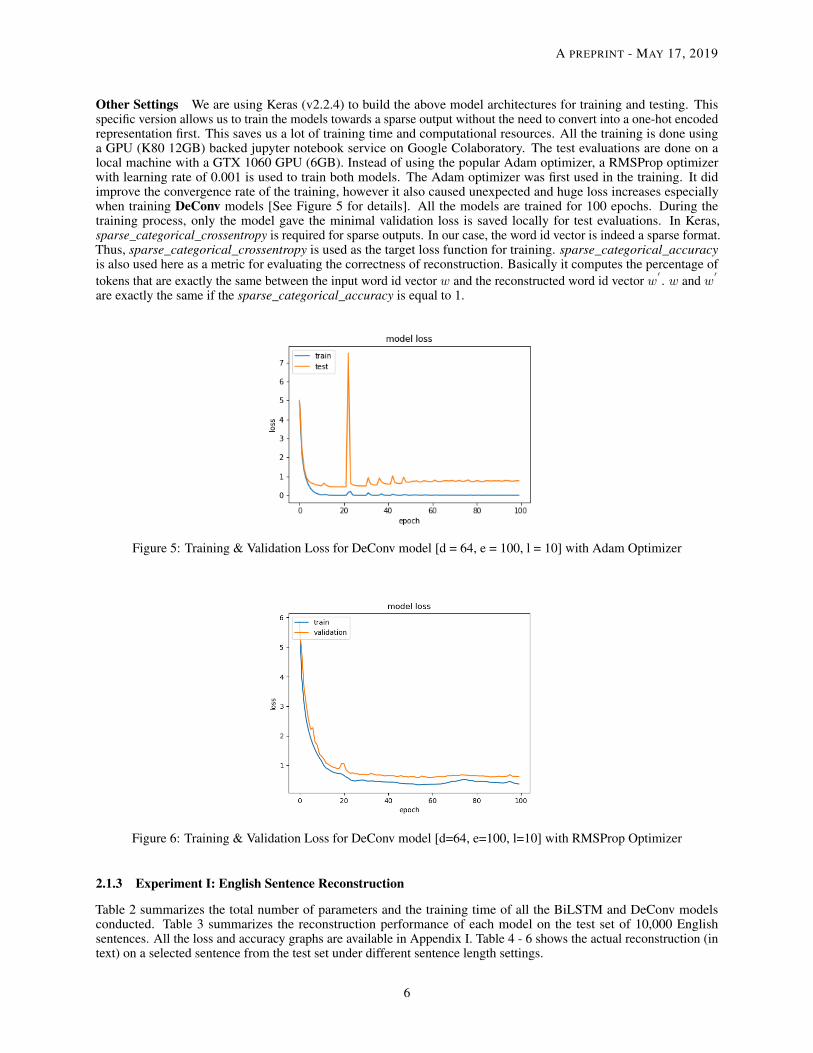
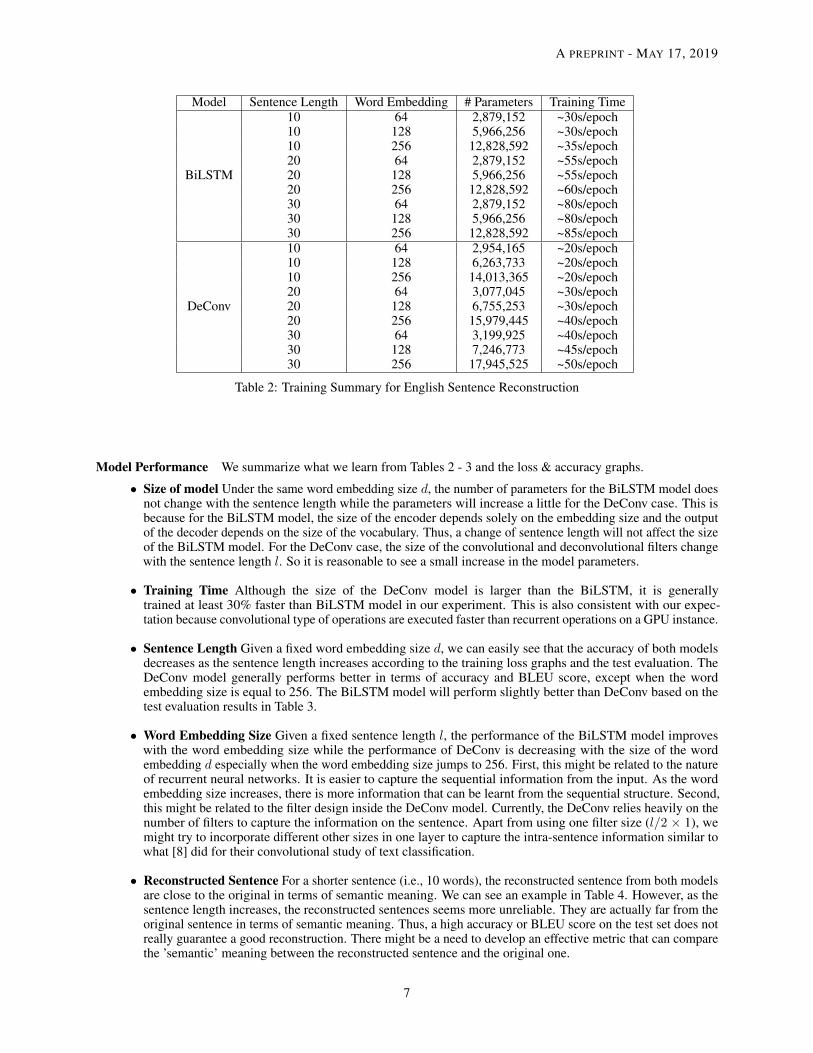
Other Settings We are using Keras (v2.2.4) to build the above model architectures for training and testing. Thisspecific version allows us to train the models towards a sparse output without the need to convert into a one-hot encodedrepresentation first. This saves us a lot of training time and computational resources. All the training is done usinga GPU (K80 12GB) backed jupyter notebook service on Google Colaboratory. The test evaluations are done on alocal machine with a GTX 1060 GPU (6GB). Instead of using the popular Adam optimizer, a RMSProp optimizerwith learning rate of 0.001 is used to train both models. The Adam optimizer was first used in the training. It didimprove the convergence rate of the training, however it also caused unexpected and huge loss increases especiallywhen training DeConv models [See Figure 5 for details]. All the models are trained for 100 epochs. During thetraining process, only the model gave the minimal validation loss is saved locally for test evaluations. In Keras,sparse_categorical_crossentropy is required for sparse outputs. In our case, the word id vector is indeed a sparse format.Thus, sparse_categorical_crossentropy is used as the target loss function for training. sparse_categorical_accuracyis also used here as a metric for evaluating the correctness of reconstruction. Basically it computes the percentage oftokens that are exactly the same between the input word id vector w and the reconstructed word id vector w
′. w and w
′
are exactly the same if the sparse_categorical_accuracy is equal to 1.
Figure 5: Training & Validation Loss for DeConv model [d = 64, e = 100, l = 10] with Adam Optimizer
Figure 6: Training & Validation Loss for DeConv model [d=64, e=100, l=10] with RMSProp Optimizer
2.1.3 Experiment I: English Sentence Reconstruction
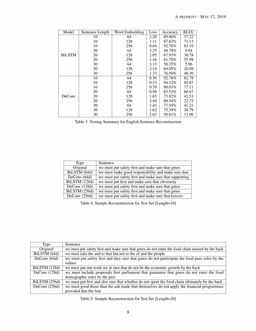
Table 2 summarizes the total number of parameters and the training time of all the BiLSTM and DeConv modelsconducted. Table 3 summarizes the reconstruction performance of each model on the test set of 10,000 Englishsentences. All the loss and accuracy graphs are available in Appendix I. Table 4 - 6 shows the actual reconstruction (intext) on a selected sentence from the test set under different sentence length settings.
6
A PREPRINT - MAY 17, 2019
Model Sentence Length Word Embedding # Parameters Training Time
BiLSTM
10 64 2,879,152 ~30s/epoch10 128 5,966,256 ~30s/epoch10 256 12,828,592 ~35s/epoch20 64 2,879,152 ~55s/epoch20 128 5,966,256 ~55s/epoch20 256 12,828,592 ~60s/epoch30 64 2,879,152 ~80s/epoch30 128 5,966,256 ~80s/epoch30 256 12,828,592 ~85s/epoch
DeConv
10 64 2,954,165 ~20s/epoch10 128 6,263,733 ~20s/epoch10 256 14,013,365 ~20s/epoch20 64 3,077,045 ~30s/epoch20 128 6,755,253 ~30s/epoch20 256 15,979,445 ~40s/epoch30 64 3,199,925 ~40s/epoch30 128 7,246,773 ~45s/epoch30 256 17,945,525 ~50s/epoch
Table 2: Training Summary for English Sentence Reconstruction
Model Performance We summarize what we learn from Tables 2 - 3 and the loss & accuracy graphs.
• Size of model Under the same word embedding size d, the number of parameters for the BiLSTM model doesnot change with the sentence length while the parameters will increase a little for the DeConv case. This isbecause for the BiLSTM model, the size of the encoder depends solely on the embedding size and the outputof the decoder depends on the size of the vocabulary. Thus, a change of sentence length will not affect the sizeof the BiLSTM model. For the DeConv case, the size of the convolutional and deconvolutional filters changewith the sentence length l. So it is reasonable to see a small increase in the model parameters.
• Training Time Although the size of the DeConv model is larger than the BiLSTM, it is generallytrained at least 30% faster than BiLSTM model in our experiment. This is also consistent with our expec-tation because convolutional type of operations are executed faster than recurrent operations on a GPU instance.
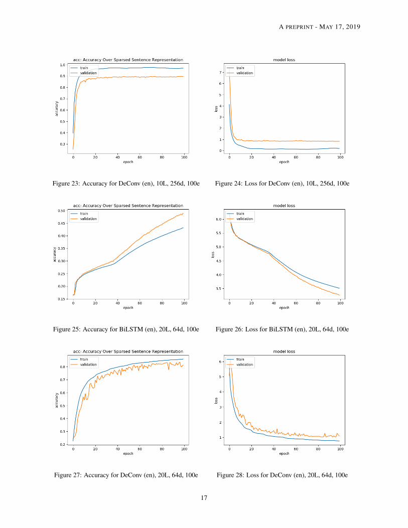
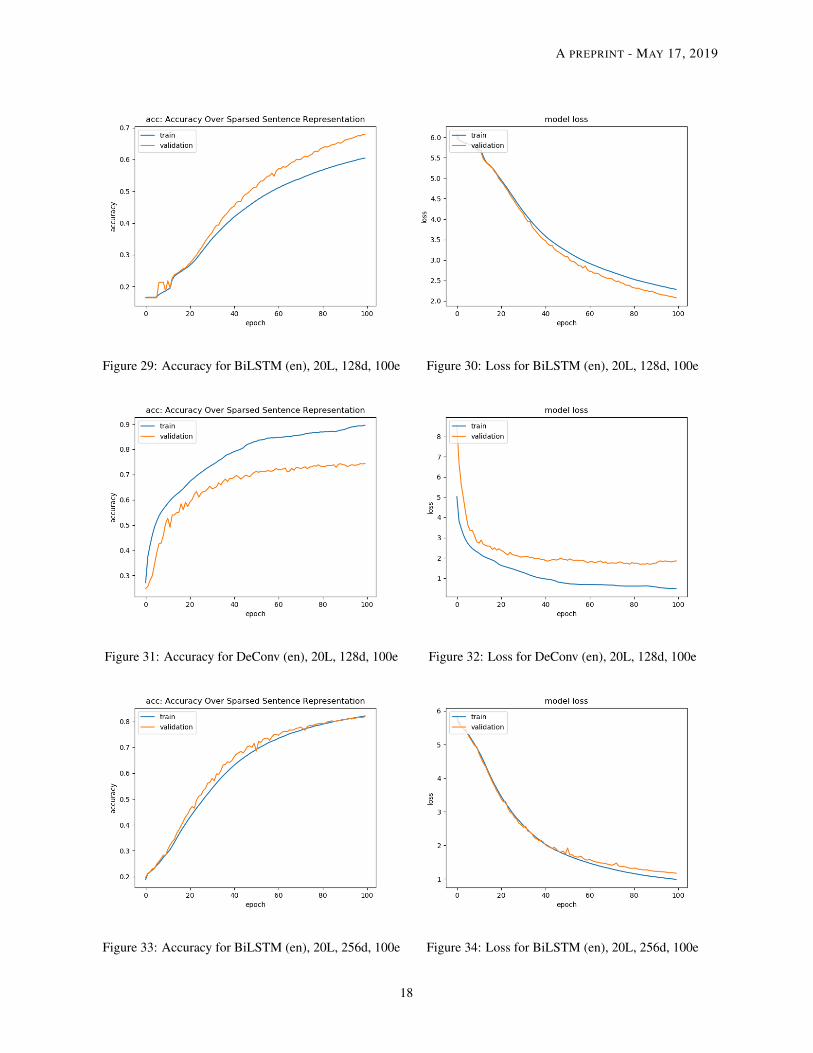
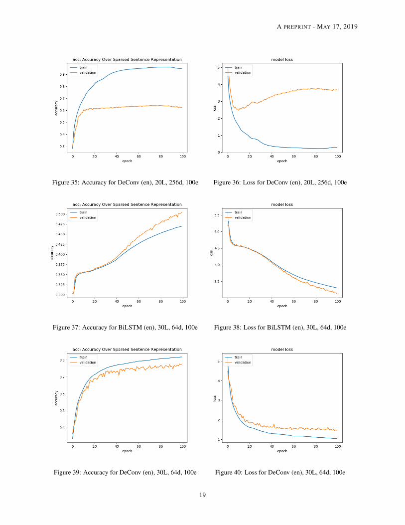
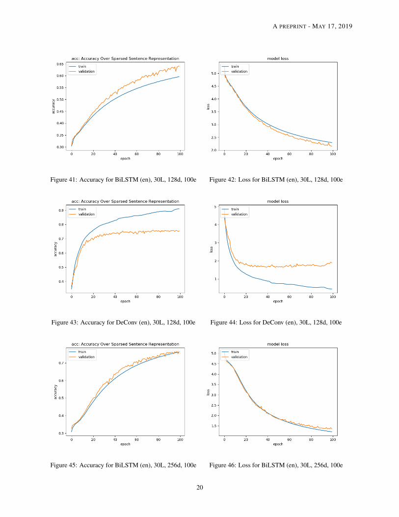
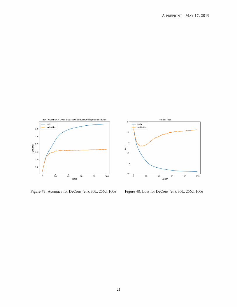
• Sentence Length Given a fixed word embedding size d, we can easily see that the accuracy of both modelsdecreases as the sentence length increases according to the training loss graphs and the test evaluation. TheDeConv model generally performs better in terms of accuracy and BLEU score, except when the wordembedding size is equal to 256. The BiLSTM model will perform slightly better than DeConv based on thetest evaluation results in Table 3.
• Word Embedding Size Given a fixed sentence length l, the performance of the BiLSTM model improveswith the word embedding size while the performance of DeConv is decreasing with the size of the wordembedding d especially when the word embedding size jumps to 256. First, this might be related to the natureof recurrent neural networks. It is easier to capture the sequential information from the input. As the wordembedding size increases, there is more information that can be learnt from the sequential structure. Second,this might be related to the filter design inside the DeConv model. Currently, the DeConv relies heavily on thenumber of filters to capture the information on the sentence. Apart from using one filter size (l/2 × 1), wemight try to incorporate different other sizes in one layer to capture the intra-sentence information similar towhat [8] did for their convolutional study of text classification.
• Reconstructed Sentence For a shorter sentence (i.e., 10 words), the reconstructed sentence from both modelsare close to the original in terms of semantic meaning. We can see an example in Table 4. However, as thesentence length increases, the reconstructed sentences seems more unreliable. They are actually far from theoriginal sentence in terms of semantic meaning. Thus, a high accuracy or BLEU score on the test set does notreally guarantee a good reconstruction. There might be a need to develop an effective metric that can comparethe ’semantic’ meaning between the reconstructed sentence and the original one.
7
A PREPRINT - MAY 17, 2019
Model Sentence Length Word Embedding Loss Accuracy BLEU
BiLSTM
10 64 2.20 69.00% 37.2210 128 1.11 87.62% 71.1310 256 0.64 92.76% 83.1020 64 3.25 48.78% 9.8420 128 2.05 67.93% 30.7820 256 1.16 81.79% 55.9830 64 3.13 50.35% 5.9630 128 2.14 64.05% 20.0930 256 1.33 76.50% 40.30
DeConv
10 64 0.56 92.78% 82.7810 128 0.53 94.12% 85.8710 256 0.79 90.03% 77.1120 64 0.99 83.53% 60.6720 128 1.65 73.82% 42.5320 256 2.44 60.34% 22.7230 64 1.43 77.54% 41.2130 128 1.62 75.39% 36.7930 256 2.63 58.81% 13.96
Table 3: Testing Summary for English Sentence Reconstruction
Type SentenceOriginal we must put safety first and make sure that gmos
BiLSTM (64d) we must make good responsibility and make sure thatDeConv (64d) we must put safety first and make sure that supporting
BiLSTM (128d) we must put first and make sure that obviouslyDeConv (128d) we must put safety first and make sure that gmosBiLSTM (256d) we must put safety first and make sure that gmosDeConv (256d) we must put safety first and make sure that kosovo
Table 4: Sample Reconstruction for Test Set [Length=10]
Type SentenceOriginal we must put safety first and make sure that gmos do not enter the food chain unseen by the back
BiLSTM (64d) we must take the and to that but not to the of and the peopleDeConv (64d) we must put safety first and they sure that gmos do not participate the food pure roles by the
reduceBiLSTM (128d) we must put our work we at sure that do not be the economic growth by the backDeConv (128d) we must include proposals first parliament that guarantee that gmos do not enter the food
demographic roles by the pastBiLSTM (256d) we must put first and also sure that whether do not spent the food chain ultimately by the backDeConv (256d) we must good those than the ask made that themselves do not apply the financial programmes
provided that the fear
Table 5: Sample Reconstruction for Test Set [Length=20]
8
A PREPRINT - MAY 17, 2019
Type SentenceOriginal we must put safety first and make sure that gmos do not enter the food chain unseen by the back
doorBiLSTM (64d) we must support on of i to that we not to the and by theDeConv (64d) we must been considered whether and make sure that gmos do not enter the food donor treatment
the number ofBiLSTM (128d) we must be an first i ask sure that not the food safety on by the backDeConv (128d) we must set act by and make whether that birth does not keep the food environment in by the
million storageBiLSTM (256d) we must be its first i make sure that us will not improve the food chain safety by the back upDeConv (256d) we must admit that what who to how that europe who to across the foreign environment although
at great basis from
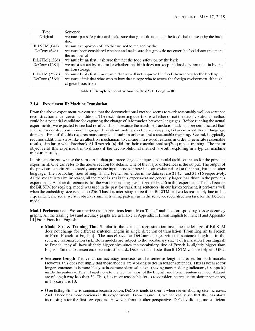
Table 6: Sample Reconstruction for Test Set [Length=30]
2.1.4 Experiment II: Machine Translation
From the above experiment, we can see that the deconvolutional method seems to work reasonably well on sentencereconstruction under certain conditions. The next interesting question is whether or not the deconvolutional methodcould be a potential candidate for capturing the change of information between languages. Before running the actualexperiments, we expected to see bad results. This is because the machine translation task is more complicated thansentence reconstruction in one language. It is about finding an effective mapping between two different languagedomains. First of all, this requires more samples to train in order to find a reasonable mapping. Second, it typicallyrequires additional steps like an attention mechanism to capture intra-word features in order to generate reasonableresults, similar to what Facebook AI Research [6] did for their convolutional seq2seq model training. The majorobjective of this experiment is to discuss if the deconvolutional method is worth exploring in a typical machinetranslation study.
In this experiment, we use the same set of data pre-processing techniques and model architectures as for the previousexperiment. One can refer to the above section for details. One of the major differences is the output. The output ofthe previous experiment is exactly same as the input, however here it is somewhat related to the input, but in anotherlanguage. The vocabulary sizes of English and French sentences in the data set are 21,424 and 31,816 respectively.As the vocabulary size increases, all the model sizes in this experiment are generally larger than those in the previousexperiments. Another difference is that the word embedding size is fixed to be 256 in this experiment. This is becausethe BiLSTM (or seq2seq) model was used in the past for translating sentences. In our last experiment, it performs wellwhen the embedding size is equal to 256. Thus it is interesting to see if the BiLSTM still works reasonably fine in thisexperiment, and see if we still observes similar training patterns as in the sentence reconstruction task for the DeConvmodel.
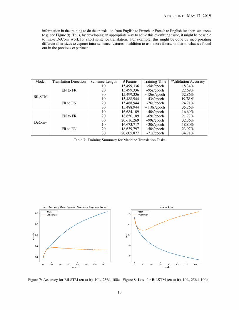
Model Performance We summarize the observations learnt from Table 7 and the corresponding loss & accuracygraphs. All the training loss and accuracy graphs are available in Appendix II [From English to French] and AppendixIII [From French to English].
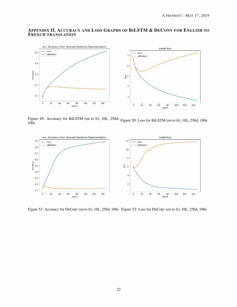
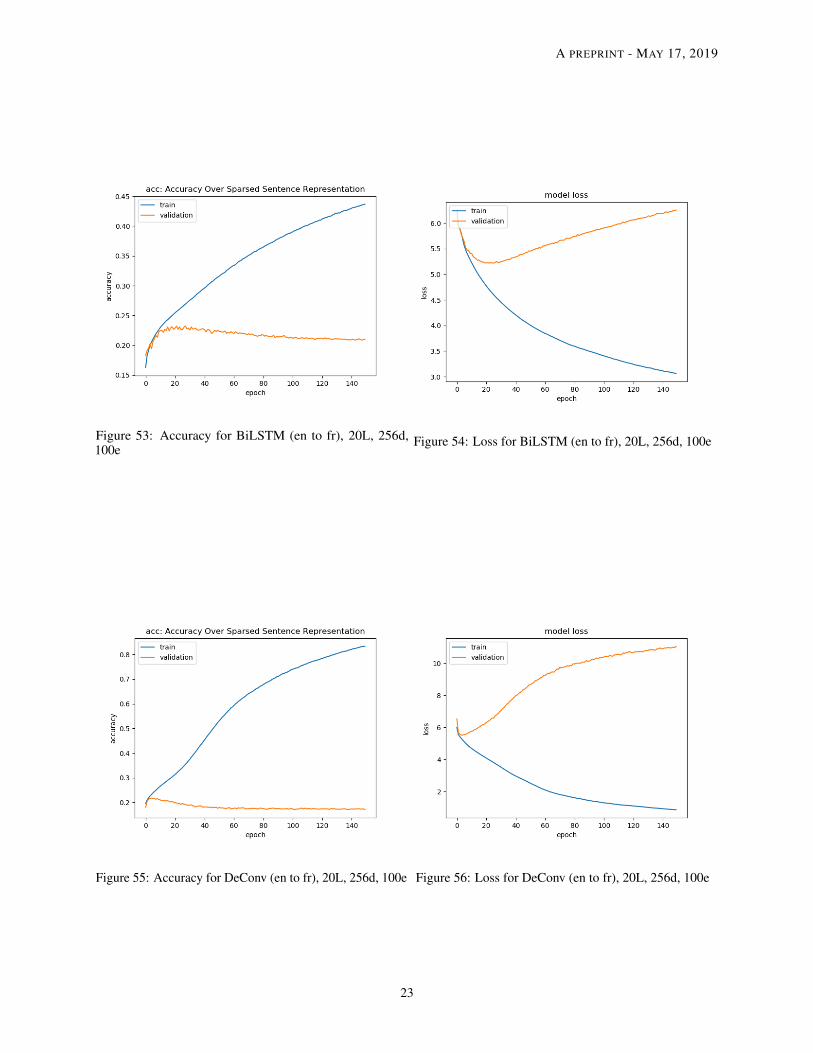
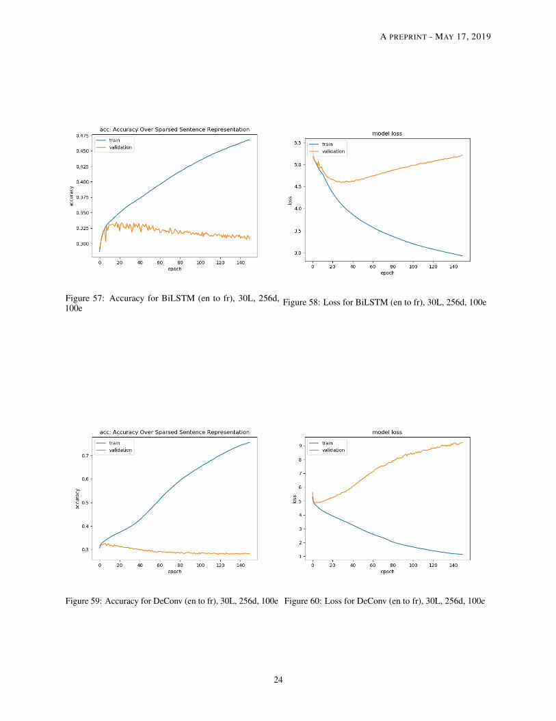
• Modal Size & Training Time Similar to the sentence reconstruction task, the model size of BiLSTMdoes not change for different sentence lengths in single direction of translation [From English to Frenchor From French to English]. The model size for DeConv changes with the sentence length as in thesentence reconstruction task. Both models are subject to the vocabulary size. For translation from Englishto French, they all have slightly bigger size since the vocabulary size of French is slightly bigger thanEnglish. Similar to the sentence reconstruction task, DeConv trains faster than BiLSTM with the help of a GPU.
• Sentence Length The validation accuracy increases as the sentence length increases for both models.However, this does not imply that those models are working better in longer sentences. This is because forlonger sentences, it is more likely to have more identical tokens (having more padding indicators, i.e. <pad>)inside the sentence. This is largely due to the fact that most of the English and French sentences in our data setare of length way less than 30. Thus, it is more reasonable for us to consider the results for shorter sentences,in this case it is 10.
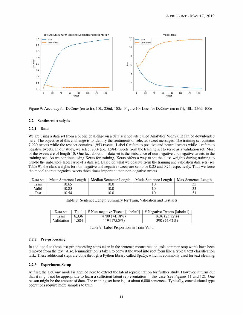
• Overfitting Similar to sentence reconstruction, DeConv tends to overfit when the emebdding size increases.And it becomes more obvious in this experiment. From Figure 10, we can easily see that the loss startsincreasing after the first few epochs. However, from another perspective, DeConv did capture sufficient
9
A PREPRINT - MAY 17, 2019
information in the training to do the translation from English to French or French to English for short sentences(e.g. see Figure 9). Thus, by developing an appropriate way to solve this overfitting issue, it might be possibleto make DeConv work for short sentence translation. For example, this might be done by incorporatingdifferent filter sizes to capture intra-sentence features in addition to usin more filters, similar to what we foundout in the previous experiment.
Model Translation Direction Sentence Length # Params Training Time *Validation Accuracy
BiLSTM
EN to FR10 15,499,336 ~54s/epoch 18.34%20 15,499,336 ~95s/epoch 22.69%30 15,499,336 ~136s/epoch 32.86%
FR to EN10 15,488,944 ~43s/epoch 19.78 %20 15,488,944 ~76s/epoch 24.71%30 15,488,944 ~110s/epoch 35.26%
DeConv
EN to FR10 16,684,109 ~40s/epoch 16.69%20 18,650,189 ~69s/epoch 21.77%30 20,616,269 ~99s/epoch 32.36%
FR to EN10 16,673,717 ~30s/epoch 18.80%20 18,639,797 ~50s/epoch 23.97%30 20,605,877 ~71s/epoch 34.71%
Table 7: Training Summary for Machine Translation Tasks
Figure 7: Accuracy for BiLSTM (en to fr), 10L, 256d, 100e Figure 8: Loss for BiLSTM (en to fr), 10L, 256d, 100e
10
A PREPRINT - MAY 17, 2019
Figure 9: Accuracy for DeConv (en to fr), 10L, 256d, 100e Figure 10: Loss for DeConv (en to fr), 10L, 256d, 100e
2.2 Sentiment Analysis
2.2.1 Data
We are using a data set from a public challenge on a data science site called Analytics Vidhya. It can be downloadedhere. The objective of this challenge is to identify the sentiments of selected tweet messages. The training set contains7,920 tweets while the test set contains 1,953 tweets. Label 0 refers to positive and neutral tweets while 1 refers tonegative tweets. In our study, we select 20% (i.e. 1,584) tweets from the training set to serve as a validation set. Mostof the tweets are of length 10. One fact about this data set is the imbalance of non-negative and negative tweets in thetraining set. As we continue using Keras for training, Keras offers a way to set the class weights during training tohandle the imbalance label issue of a data set. Based on what we observe from the training and validation data sets (seeTable 9), the class weights for non-negative and negative tweets are set to be 0.25 and 0.75 respectively. Thus we forcethe model to treat negative tweets three times important than non-negative tweets.
Data set Mean Sentence Length Median Sentence Length Mode Sentence Length Max Sentence LengthTrain 10.65 10.0 10 35Valid 10.85 10.0 10 33Test 10.54 10.0 10 31
Table 8: Sentence Length Summary for Train, Validation and Test sets
Data set Total # Non-negative Tweets [label=0] # Negative Tweets [label=1]Train 6,336 4700 (74.18%) 1636 (25.82%)
Validation 1,584 1194 (75.8%) 390 (24.62%)
Table 9: Label Proportion in Train Valid
2.2.2 Pre-processing
In additional to those text pre-processing steps taken in the sentence reconstruction task, common stop words have beenremoved from the text. Also, lemmatization is taken to convert the word into root form like a typical text classificationtask. These additional steps are done through a Python library called SpaCy, which is commonly used for text cleaning.
2.2.3 Experiment Setup
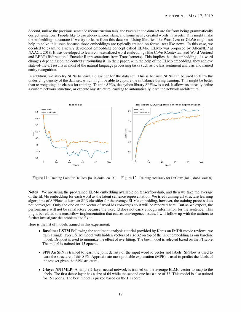
At first, the DeConv model is applied here to extract the latent representation for further study. However, it turns outthat it might not be appropriate to learn a sufficient latent representation in this case (see Figures 11 and 12). Onereason might be the amount of data. The training set here is just about 6,000 sentences. Typically, convolutional typeoperations require more samples to train.
11
A PREPRINT - MAY 17, 2019
Second, unlike the previous sentence reconstruction task, the tweets in the data set are far from being grammaticallycorrect sentences. People like to use abbreviations, slang and some newly created words in tweets. This might makethe embedding inaccurate if we try to learn from this data set. Using libraries like Word2vec or GloVe might nothelp to solve this issue because those embeddings are typically trained on formal text like news. In this case, wedecided to examine a newly developed embedding concept called ELMo. ELMo was proposed by AllenNLP atNAACL 2018. It was developed to learn contextualized word embeddings like CoVe (Contextualized Word Vectors)and BERT (Bidirectional Encoder Representations from Transformers). This implies that the embedding of a wordchanges depending on the context surrounding it. In their paper, with the help of the ELMo embedding, they achievestate-of-the-art results in most of the natural language processing tasks such as 5-class sentiment analysis and namedentity recognition.
In addition, we also try SPNs to learn a classifier for the data set. This is because SPNs can be used to learn theunderlying density of the data set, which might be able to capture the imbalance during training. This might be betterthan re-weighting the classes for training. To train SPNs, the python library SPFlow is used. It allows us to easily definea custom network structure, or execute any structure learning to automatically learn the network architecture.
Figure 11: Training Loss for DeConv [l=10, d=64, e=100] Figure 12: Training Accuracy for DeConv [l=10, d=64, e=100]
Notes We are using the pre-trained ELMo embedding available on tensorflow-hub, and then we take the averageof the ELMo embedding for each word as the latent sentence representation. We tried running all structure learningalgorithms of SPFlow to learn an SPN classifier for the average ELMo embedding, however, the training process doesnot converges. Only the one on the vector of word ids converges so it will be reported here. But as we expect, theperformance will not be satisfactory because the word id does not carry enough information for the sentence. Thismight be related to a tensorflow implementation that causes convergence issues. I will follow up with the authors tofurther investigate the problem and fix it.
Here is the list of models trained in this experiment:
• Baseline: LSTM Following the sentiment analysis tutorial provided by Keras on IMDB movie reviews, wetrain a single layer LSTM model with hidden vectors of size 32 on top of the input embedding as our baselinemodel. Dropout is used to minimize the effect of overfitting. The best model is selected based on the F1 score.The model is trained for 15 epochs.
• SPN An SPN is trained to learn the joint density of the input word id vector and labels. SPFlow is used tolearn the structure of this SPN. Approximate most probable explanation (MPE) is used to predict the labels ofthe test set given the SPN structure.
• 2-layer NN [MLP] A simple 2-layer neural network is trained on the average ELMo vector to map to thelabels. The first dense layer has a size of 64 while the second one has a size of 32. This model is also trainedfor 15 epochs. The best model is picked based on the F1 score.
12
A PREPRINT - MAY 17, 2019
• Logistic Regression A simple logistic regression model is trained on the average ELMo vector.
2.2.4 Experimental Results
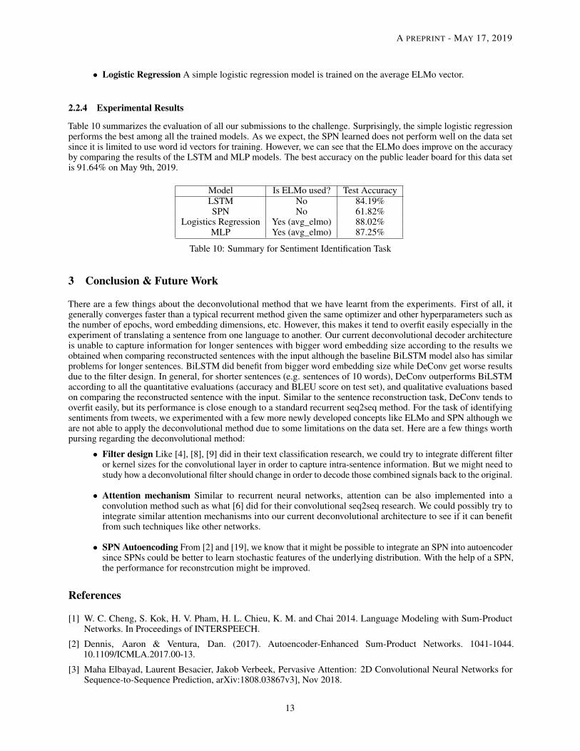
Table 10 summarizes the evaluation of all our submissions to the challenge. Surprisingly, the simple logistic regressionperforms the best among all the trained models. As we expect, the SPN learned does not perform well on the data setsince it is limited to use word id vectors for training. However, we can see that the ELMo does improve on the accuracyby comparing the results of the LSTM and MLP models. The best accuracy on the public leader board for this data setis 91.64% on May 9th, 2019.
Model Is ELMo used? Test AccuracyLSTM No 84.19%SPN No 61.82%
Logistics Regression Yes (avg_elmo) 88.02%MLP Yes (avg_elmo) 87.25%
Table 10: Summary for Sentiment Identification Task
3 Conclusion & Future Work
There are a few things about the deconvolutional method that we have learnt from the experiments. First of all, itgenerally converges faster than a typical recurrent method given the same optimizer and other hyperparameters such asthe number of epochs, word embedding dimensions, etc. However, this makes it tend to overfit easily especially in theexperiment of translating a sentence from one language to another. Our current deconvolutional decoder architectureis unable to capture information for longer sentences with bigger word embedding size according to the results weobtained when comparing reconstructed sentences with the input although the baseline BiLSTM model also has similarproblems for longer sentences. BiLSTM did benefit from bigger word embedding size while DeConv get worse resultsdue to the filter design. In general, for shorter sentences (e.g. sentences of 10 words), DeConv outperforms BiLSTMaccording to all the quantitative evaluations (accuracy and BLEU score on test set), and qualitative evaluations basedon comparing the reconstructed sentence with the input. Similar to the sentence reconstruction task, DeConv tends tooverfit easily, but its performance is close enough to a standard recurrent seq2seq method. For the task of identifyingsentiments from tweets, we experimented with a few more newly developed concepts like ELMo and SPN although weare not able to apply the deconvolutional method due to some limitations on the data set. Here are a few things worthpursing regarding the deconvolutional method:
• Filter design Like [4], [8], [9] did in their text classification research, we could try to integrate different filteror kernel sizes for the convolutional layer in order to capture intra-sentence information. But we might need tostudy how a deconvolutional filter should change in order to decode those combined signals back to the original.
• Attention mechanism Similar to recurrent neural networks, attention can be also implemented into aconvolution method such as what [6] did for their convolutional seq2seq research. We could possibly try tointegrate similar attention mechanisms into our current deconvolutional architecture to see if it can benefitfrom such techniques like other networks.
• SPN Autoencoding From [2] and [19], we know that it might be possible to integrate an SPN into autoencodersince SPNs could be better to learn stochastic features of the underlying distribution. With the help of a SPN,the performance for reconstrcution might be improved.
References
[1] W. C. Cheng, S. Kok, H. V. Pham, H. L. Chieu, K. M. and Chai 2014. Language Modeling with Sum-ProductNetworks. In Proceedings of INTERSPEECH.
[2] Dennis, Aaron & Ventura, Dan. (2017). Autoencoder-Enhanced Sum-Product Networks. 1041-1044.10.1109/ICMLA.2017.00-13.
[3] Maha Elbayad, Laurent Besacier, Jakob Verbeek, Pervasive Attention: 2D Convolutional Neural Networks forSequence-to-Sequence Prediction, arXiv:1808.03867v3], Nov 2018.
13
A PREPRINT - MAY 17, 2019
[4] Baotian Hu, Zhengdong Lu, Hang Li, and Qingcai Chen. Convolutional neural network architectures for matchingnatural language sentences. In NIPS, 2014.
[5] Zhe Gan, Yunchen Pu, Henao Ricardo, Chunyuan Li, Xiaodong He, and Lawrence Carin. Learning generic sentencerepresentations using convolutional neural networks. In EMNLP, 2017.
[6] Jonas Gehring, Michael Auli, David Grangier, Yann Dauphin, A Convolutional Encoder Model for Neural MachineTranslation, Proceedings of the 55th Annual Meeting of the Association for Computational Linguistics (Volume 1:Long Papers), Jul 2017.
[7] Rie Johnson and Tong Zhang. Effective use of word order for text categorization with convolutional neural networks.In NAACL HLT, 2015.
[8] Nal Kalchbrenner, Edward Grefenstette, and Phil Blunsom. A convolutional neural network for modelling sentences.In ACL, 2014
[9] Yoon Kim. Convolutional neural networks for sentence classification. In EMNLP, 2014.[10] P. Koehn. 2005. Europarl: A parallel corpus for statistical machine translation. In Machine Translation Summit X,
pages 79–86, Phuket, Thailand.[11] T. Mikolov, M. Karafiat, J. Cernocky, and S. Khudanpur, “Recurrent neural network based language model,” in
INTERSPEECH, 2010.[12] Tomas Mikolov, Kai Chen, Greg Corrado, and Jeffrey Dean. 2013. Efficient estimation of word representations in
vector space. In Workshop Proceedings of the International Conference on Learning Representations.[13] Hyeonwoo Noh, Seunghoon Hong, Bohyung Han, Learning Deconvolution Network for Semantic Segmentation,
arXiv:1505.04366v1, May 2015.[14] Barak Oshri and Nishith Khandwala. 2014. There and Back Again: Autoencoders for Textual Reconstruction.
Retrieved from https://cs224d.stanford.edu/reports/OshriBarak.pdf.[15] Hoifung Poon and Pedro Domingos. Sum-product networks: A new deep architecture. In UAI, pages 2551–2558,
2011.[16] Stanislau Semeniuta, Aliaksei Severyn, and Erhardt Barth. A Hybrid Convolutional Variational Autoencoder for
Text Generation. arXiv, February 2017.[17] Karen Simonyan and Andrew Zisserman. Very deep convolutional networks for large-scale image recognition. In
ICLR, 2015.[18] Ashish Vaswani, Noam Shazeer, Niki Parmar, Jakob Uszkoreit, Llion Jones, Aidan N Gomez, Lukasz Kaiser, and
Illia Polosukhin. 2017. Attention is all you need. NIPS.[19] Vergari, Antonio & Peharz, Robert & Di Mauro, Nicola & Molina, Alejandro & Kersting, Kristian & Esposito,
Floriana. (2018). Sum-Product Autoencoding: Encoding and Decoding Representations using Sum-ProductNetworks. AAAI-18.
[20] Yizhe Zhang, Dinghan Shen, Guoyin Wang, Zhe Gan, Ricardo Henao, and Lawrence Carin. 2017b. Deconvolu-tional paragraph representation learning. NIPS.
14
A PREPRINT - MAY 17, 2019
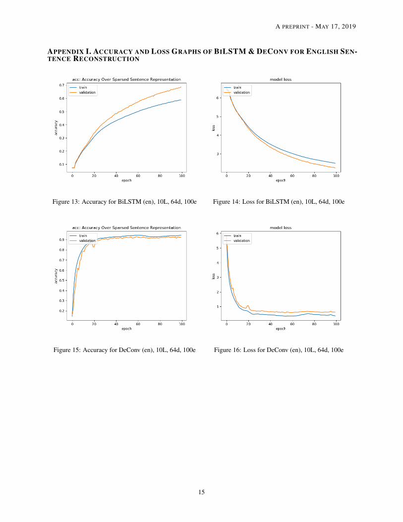
APPENDIX I. ACCURACY AND LOSS GRAPHS OF BILSTM & DECONV FOR ENGLISH SEN-TENCE RECONSTRUCTION
Figure 13: Accuracy for BiLSTM (en), 10L, 64d, 100e Figure 14: Loss for BiLSTM (en), 10L, 64d, 100e
Figure 15: Accuracy for DeConv (en), 10L, 64d, 100e Figure 16: Loss for DeConv (en), 10L, 64d, 100e
15
A PREPRINT - MAY 17, 2019
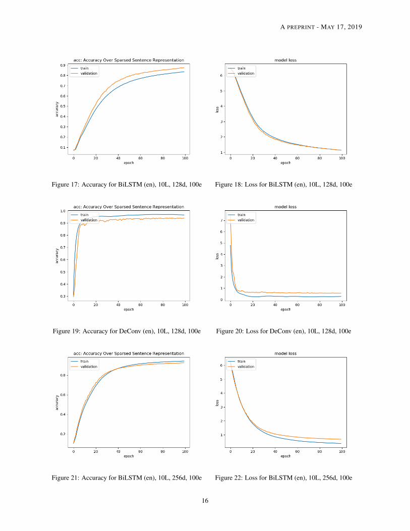
Figure 17: Accuracy for BiLSTM (en), 10L, 128d, 100e Figure 18: Loss for BiLSTM (en), 10L, 128d, 100e
Figure 19: Accuracy for DeConv (en), 10L, 128d, 100e Figure 20: Loss for DeConv (en), 10L, 128d, 100e
Figure 21: Accuracy for BiLSTM (en), 10L, 256d, 100e Figure 22: Loss for BiLSTM (en), 10L, 256d, 100e
16
A PREPRINT - MAY 17, 2019
Figure 23: Accuracy for DeConv (en), 10L, 256d, 100e Figure 24: Loss for DeConv (en), 10L, 256d, 100e
Figure 25: Accuracy for BiLSTM (en), 20L, 64d, 100e Figure 26: Loss for BiLSTM (en), 20L, 64d, 100e
Figure 27: Accuracy for DeConv (en), 20L, 64d, 100e Figure 28: Loss for DeConv (en), 20L, 64d, 100e
17
A PREPRINT - MAY 17, 2019
Figure 29: Accuracy for BiLSTM (en), 20L, 128d, 100e Figure 30: Loss for BiLSTM (en), 20L, 128d, 100e
Figure 31: Accuracy for DeConv (en), 20L, 128d, 100e Figure 32: Loss for DeConv (en), 20L, 128d, 100e
Figure 33: Accuracy for BiLSTM (en), 20L, 256d, 100e Figure 34: Loss for BiLSTM (en), 20L, 256d, 100e
18
A PREPRINT - MAY 17, 2019
Figure 35: Accuracy for DeConv (en), 20L, 256d, 100e Figure 36: Loss for DeConv (en), 20L, 256d, 100e
Figure 37: Accuracy for BiLSTM (en), 30L, 64d, 100e Figure 38: Loss for BiLSTM (en), 30L, 64d, 100e
Figure 39: Accuracy for DeConv (en), 30L, 64d, 100e Figure 40: Loss for DeConv (en), 30L, 64d, 100e
19
A PREPRINT - MAY 17, 2019
Figure 41: Accuracy for BiLSTM (en), 30L, 128d, 100e Figure 42: Loss for BiLSTM (en), 30L, 128d, 100e
Figure 43: Accuracy for DeConv (en), 30L, 128d, 100e Figure 44: Loss for DeConv (en), 30L, 128d, 100e
Figure 45: Accuracy for BiLSTM (en), 30L, 256d, 100e Figure 46: Loss for BiLSTM (en), 30L, 256d, 100e
20
A PREPRINT - MAY 17, 2019
Figure 47: Accuracy for DeConv (en), 30L, 256d, 100e Figure 48: Loss for DeConv (en), 30L, 256d, 100e
21
A PREPRINT - MAY 17, 2019
APPENDIX II. ACCURACY AND LOSS GRAPHS OF BILSTM & DECONV FOR ENGLISH TOFRENCH TRANSLATION
Figure 49: Accuracy for BiLSTM (en to fr), 10L, 256d,100e
Figure 50: Loss for BiLSTM (en to fr), 10L, 256d, 100e
Figure 51: Accuracy for DeConv (en to fr), 10L, 256d, 100e Figure 52: Loss for DeConv (en to fr), 10L, 256d, 100e
22
A PREPRINT - MAY 17, 2019
Figure 53: Accuracy for BiLSTM (en to fr), 20L, 256d,100e
Figure 54: Loss for BiLSTM (en to fr), 20L, 256d, 100e
Figure 55: Accuracy for DeConv (en to fr), 20L, 256d, 100e Figure 56: Loss for DeConv (en to fr), 20L, 256d, 100e
23
A PREPRINT - MAY 17, 2019
Figure 57: Accuracy for BiLSTM (en to fr), 30L, 256d,100e
Figure 58: Loss for BiLSTM (en to fr), 30L, 256d, 100e
Figure 59: Accuracy for DeConv (en to fr), 30L, 256d, 100e Figure 60: Loss for DeConv (en to fr), 30L, 256d, 100e
24
A PREPRINT - MAY 17, 2019
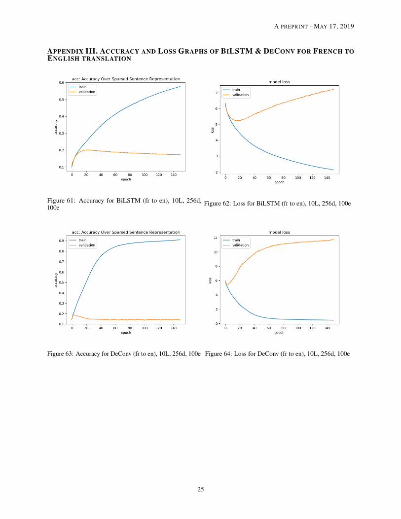
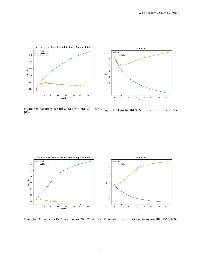
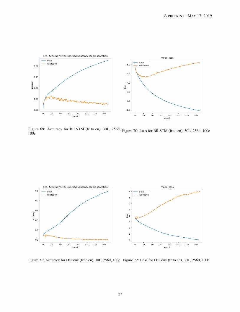
APPENDIX III. ACCURACY AND LOSS GRAPHS OF BILSTM & DECONV FOR FRENCH TOENGLISH TRANSLATION
Figure 61: Accuracy for BiLSTM (fr to en), 10L, 256d,100e
Figure 62: Loss for BiLSTM (fr to en), 10L, 256d, 100e
Figure 63: Accuracy for DeConv (fr to en), 10L, 256d, 100e Figure 64: Loss for DeConv (fr to en), 10L, 256d, 100e
25
A PREPRINT - MAY 17, 2019
Figure 65: Accuracy for BiLSTM (fr to en), 20L, 256d,100e
Figure 66: Loss for BiLSTM (fr to en), 20L, 256d, 100e
Figure 67: Accuracy for DeConv (fr to en), 20L, 256d, 100e Figure 68: Loss for DeConv (fr to en), 20L, 256d, 100e
26
A PREPRINT - MAY 17, 2019
Figure 69: Accuracy for BiLSTM (fr to en), 30L, 256d,100e
Figure 70: Loss for BiLSTM (fr to en), 30L, 256d, 100e
Figure 71: Accuracy for DeConv (fr to en), 30L, 256d, 100e Figure 72: Loss for DeConv (fr to en), 30L, 256d, 100e
27