Palaeoglaciology of an ice sheet through a glacial cycle ... 2006 readings/Scandinavia and... ·...

*Corresponding author. Tel.: #00-44-650-4844.E-mail address: [email protected] (G.S. Boulton).

Quaternary Science Reviews 20 (2001) 591}625

Palaeoglaciology of an ice sheet through a glacial cycle:the European ice sheet through the Weichselian

G.S. Boulton*, P. Dongelmans, M. Punkari, M. BroadgateDepartment of Geology and Geophysics, University of Edinburgh, Grant Institute, Kings Buildings, Edinburgh, EH9 3JW, UK

Abstract

Satellite images provide unique means of identifying large-scale #ow-generated lineations produced by former ice sheets. They canbe interpreted to reconstruct the major elements which make up the integrated, large-scale structure of ice sheets: ice divides; icestreams; interstream ridges; ice shelves; calving bays. The evolving palaeoglaciological structure of the European ice sheet during itsdecay from the Last Glacial Maximum (LGM) is reconstructed by reference to these components and in the context of a new mapshowing isochrons of retreat. During the retreat phase in particular the time-dependent dynamic evolution of the ice sheet and thepattern of ice stream development are reconstructed. Crossing lineations are widespread. The older ones are suggested to have formedduring molten bed phases of ice sheet growth and preserved by frozen bed conditions during the glacial maximum, particularly inareas which lay, during deglaciation, beneath ice divides and inter-ice stream ridges, both areas of slow #ow and possibly frozen bedconditions. Four phases of growth (A1 to A4) and "ve phases of decay (R1 to R5) are used to describe the major climatically anddynamically determined stages in the evolution of the ice sheet through the last glacial cycle. The growth and decay patterns are quitedi!erent and associated with major shifts in the ice divide, re#ecting growth from the Fennoscandian mountains and decay away frommarine in#uenced margins. These patterns were determined by the locations of nucleation areas; spatial patterns of climate; andcalving at marine margins.The prevalence of streaming within the retreating ice sheet suggests that the mean elevation of the ice sheetwas lower than predicted from glaciological models which do not include streaming, and that this might reconcile glaciologicalmodels and earth rheology models which infer paleao-ice sheet thickness by inverting sea level data. ( 2001 Elsevier Science Ltd. Allrights reserved.

1. Introduction

Reconstructions of the form and #ow of former icesheets have largely been based on geological evidence offeatures such as drumlins, striations and till fabrics whichre#ect the direction of ice sheet movement, rather thanfrom the more sparse moraines which indicate the loca-tions of former ice margins. In the earliest reconstruc-tions, it was generally assumed that these features weremore or less synchronous and showed the pattern of #owduring the glacial maximum (e.g. Torell, 1865; Chamber-lin, 1895; Charlesworth, 1957). The relatively few mo-raines which did exist were used to reconstruct thepattern of the last deglaciation. It was later recognisedthat the large-scale distribution of #ow-parallel featuresrepresented time transgressive events, and that ratherthan indicating the patterns of #ow at glacial maxima,they were a re#ection of the pattern of "nal ice sheetdecay (Boulton et al., 1985). Much fuller reconstructions

of patterns of deglaciation were then based on the as-sumption that, on a #at bed, most #ow-parallel featuresproduced near to the glacier terminus will be normal tothe ice margin, and that features formed in terminalpositions during the last retreat will tend to overprintearlier features (e.g. Boulton et al., 1985; Lundqvist,1986). On this basis, the continent-wide patterns of #ow-parallel lineation which had long been recognised werenow seen largely as re#ections of time transgressive pro-cesses of erosion and deposition in the terminal zone ofthe ice sheet during its "nal decay.

The recognition that large-scale sets of #ow-parallelfeatures frequently cross each other (Boulton and Clark,1990a, b) indicated that not all such lineations weregenerated close to the ice margin during "nal retreatand that many may long pre-date "nal deglaciation.LagerbaK ck (1988) and Kleman (1990) argued, respective-ly, that early Weichselian eskers and bedrock striationshave survived in Sweden without signi"cant reworkingduring Late Weichselian glaciation (see also Hatter-strand and Kleman, 1999). Such features may havesurvived the Late Weichselian glacial maximum because

0277-3791/01/$ - see front matter ( 2001 Elsevier Science Ltd. All rights reserved.PII: S 0 2 7 7 - 3 7 9 1 ( 0 0 ) 0 0 1 6 0 - 8

the ice/bed interface was frozen in the ice divide region orbecause low ice velocities in the divide region producedvery little erosion of earlier features. Discovery of thepreservation of such multiple lineation sets permits us touse geomorphological information not only to recon-struct the pattern of #ow during the "nal deglaciation,but also to reconstruct patterns of #ow during the pre-maximum and build-up stages. Boulton and Clark(1990a, b) did this for the Laurentide ice sheet, andconcluded that it had behaved in a much more dynamicway than hitherto supposed, with major and rapid shiftsof its centres of mass through the last glacial cycle.

Although the form and #ow dynamics of modern icesheets are relatively well understood, fuller understand-ing of their role in the climate system requires analysis oftheir behaviour in time as well as space. Numerical mod-elling of ice sheets can help in this, but is not an adequatesubstitute for empirically based reconstructions of thetime-dependent behaviour of past ice sheets, through anapproach which should be termed palaeoglaciology, andwhich this article attempts to illustrate. It involves threesteps:

f characterising the basic dynamic elements of an icesheet as re#ected in the glaciology of modern icesheets,

f identifying geological features which re#ect behaviourof these dynamic elements,

f interpretation and integration of these features to re-construct a palaeoglaciological narrative of long-termdynamic change.

The purpose of this article is to improve the glacialgeological reconstruction of the European ice sheet pre-sented by Boulton et al. (1985), and to use a palaeo-glaciological approach to reconstruct the dynamicbehaviour of the ice sheet through the last glacial cycle.Kleman et al. (1997) published an approach essentiallysimilar to that presented here at about the same time thatthis article was "rst submitted for publication (Novem-ber, 1997). It di!ers in two major ways from that pre-sented here. Firstly it utilises a mosaic of previouslypublished data for the shield area whereas we use a singleprimary data source for that area, that of satellite im-agery. Secondly, it is primarily concerned to identifychanges in bed conditions whereas we attempt to recon-struct some of the large-scale characteristics of the icesheet itself. Both can e!ectively be used as a basis fortesting the capacity of numerical models to simulatedi!erent aspects of the three dimensional time-dependentbehaviour of the ice sheet.

2. Data

We have used two principal data sources to plot thedistribution of large-scale glacigenic landforms within

the area of north-west Europe believed to have beenoccupied by an ice sheet during the last glacial cycle.Satellite images have been used for the inner region of theice sheet (Fennoscandia, northwestern Russia and muchof the area of Estonia, Latvia and Lithuania), and exist-ing "eldwork-based compilations for the peripheralareas (Krasnov, 1971; Chebotareva, 1977; Liedtke, 1981;Kozarski, 1986, 1988; Ehlers, 1990). In the former, MSSimages (resolution 79m) were used, with TM images(resolution 30 m) and SPOT images (resolution 10}20m)for some more detailed interpretations. Interpretationsutilise the capacity of spectral and spatial informationto discriminate between drift deposits and bedrockand between glacial landforms and bedrock features(Punkari, 1982, 1985, 1993; Boulton et al., 1985;Boulton and Clark, 1990a, b). The validity of our inter-pretations of glacial landforms has been checked, in se-lected areas, against "eld surveys where they exist butparticularly through studies of conventional aerialphotography, where there is rarely any doubt whetherparticular features are drumlins, ice smoothed rock surfa-ces or moraines. Given the scale of this study however,this can only be done for a very limited number ofexamples.

We have mapped three principle landform types:Eskers: Narrow winding ridges have been mapped,

approximately parallel to directions of ice #ow, whichcoincide with the locations of eskers marked on theexcellent detailed maps of the Norwegian, Swedish andFinnish Geological Surveys (Nordkalott project, 1986).However, the narrowness and the sinuous or relativelydisordered form of eskers makes them di$cult to identifyon the images which we have used, unless they are longand continuous, in which case their continuity aids theiridenti"cation. Our mapping therefore underestimatestheir frequency compared with the results of groundbased survey. Kleman et al. (1997) have used the distribu-tion of eskers on glaciated surfaces as an index of condi-tions at the ice/bed interface.

Moraines: Moraines form at and parallel to glaciermargins. They are less sinuous than eskers, and can varymarkedly in width along their length. This irregularitymakes them di$cult to identify from the images which wehave used. Relatively minor and discontinuous moraineswhich have been mapped on ground surveys, such as theMiddle Swedish Moraines, are di$cult to identify, butmajor or continuous moraines, such as the SalpausselkaMoraines of Finland, are easily identi"ed.

Drumlins: Satellite survey comes into its own in identi-fying straight, #ow-parallel, streamlined landforms whichoccur in "elds of mutually parallel ridges. They are quitedi!erent from the more complex forms of moraines andfrom eskers. We believe that almost all such #ow-parallelfeatures which we have mapped are sediment ridges,10's}1000's of metres in length, metres to 10's of metres inheight, and 10's to 100's of metres in width. They show

592 G.S. Boulton et al. / Quaternary Science Reviews 20 (2001) 591}625

Fig. 1. Location of the satellite images used to map glacial lineations, together with locations of conventional aerial photographs used to checksatellite interpretations. Satellite imagery has been used for the whole of the shield areas, where patterns of arable agriculture do not obscure glacialfeatures. Published ground observations have been used to cover areas beyond the shield, and limited areas in the Baltic states have been studied usingsatellite-derived data. Numbers identify images referred to in Figs. 2 and 3 and in the text.

great diversity of size and of detailed form and can all bereasonably grouped together as `drumlinsa. Our mapstend to show a greater density of drumlins than maps ofdrumlin "elds compiled from "eld surveys. Althoughsuch comparisons show that small drumlins are missedby satellite surveys, we are often able to identify drumlinsof great extent and low relief which are too large to bediscerned by "eld surveys, suggesting that in many drum-lin "elds, satellite surveys generally produce a betterestimate of the total drumlin population. Satellite surveyis also an e!ective means of identifying where changingdirections of ice #ow have created two populations ofdrumlins, in which older drumlins have been partiallyreworked to create a second, cross-cutting drumlin set(Boulton and Clark, 1990b).

The locations of the images on which our interpreta-tions are based are shown in Fig. 1. Examples of imagesand interpretations made from them are shown inFigs. 2}4. Satellite image survey has the advantages thata single operator or a small group can apply a well-de"ned set of criteria on a continental scale; that largefeatures which are often unresolveable by ground or airphoto survey can be identi"ed and that groups of individ-ually indistinct linear elements can be recomposed vis-ually into coherent patterns to infer integrated patternsof ice #ow. In our view, the level of coherent detail aboutpatterns of lineation over wide areas that can be mappedfrom satellite imagery is generally greater than hashitherto been obtained from ground surveys such asthose used by Kleman et al. (1997; see their Fig. 3).

G.S. Boulton et al. / Quaternary Science Reviews 20 (2001) 591}625 593

Fig. 2. (a) Conventional aerial photograph showing crossing lineations at Utsjoki in northern Finland. Drumlins directed towards the NNE (trendshown by large open arrows) have smaller #utes and drumlins directed towards the NE superimposed on their surfaces (trend shown by smaller "lledarrows), suggesting a clockwise rotation of ice movement of about 253. (b) A satellite image immediately to the south of (a), from f25 on Fig. 1. Theupward direction is towards 3103 and the width of the image is 130 km. A strong S}N lineation de"ned by an extensive drumlin "eld is shown in thecentral part of the image, where it overprints an older NNE trending lineation.

Satellite derived data contrasts with stratigraphic andsedimentological evidence of palaeoglaciology, whichtends only to yield information from very small areasabout glacier behaviour which was continental in scale.In this study we have plotted continent-wide spatialpatterns of #ow parallel lineations as a basis for recon-structing spatial patterns of ice sheet behaviour. It hasthe disadvantage that it only permits, at best, relativedating and has the danger that temporally separated #owevents are grouped together. It should ultimately beintegrated with stratigraphic and sedimentological data(Dongelmans, 1997).

To guard against overly subjective interpretations, theauthors have individually and independently producedinterpretations of the same areas and cross-checkedthe results. In general, we have not found substantivelydi!erent interpretations. In some areas, bedrock struc-tures show linear patterns, but many such areas can beeliminated by using existing geological and geophysicalmaps.

Figs. 3a, c and e show details of #ow-parallel lineationsobserved on satellite images at a scale of 1 : 300,000. Weterm these "rst order lineations. In some cases it is clearthat di!erent parts of the images show #ow lineationswhich could not re#ect synchronous patterns of basal ice

#ow. In some cases, lineations cross, and in some of these,it is possible to establish the relative ages of lineationsfrom satellite images (Boulton, 1987). In some, relativeages have been checked by reference to aerial photo-graphs, but in others no clear inferences of relative agecould be made.

It is not possible to show "rst-order interpretations onan ice sheet wide basis in "gures of the scale used in thisarticle. In order to show ice sheet wide patterns, threesuccessive approximations have been made:

(a) Maps of "rst-order interpretations have been gener-alised to produce second-order interpretations oflineation sets which clearly form part of spatiallyintegrated groups that can be summarised by a seriesof lines which are longer than the original lines repres-enting individual geomorphological features (Figs. 3b,d and f ). Many show several crossing lineation sets.

(b) The second-order interpretations have been furthercompiled to produce third-order lineation maps oflarge sectors of the ice sheet (Fig. 4).

(c) These have been further simpli"ed to produce fourth-order maps of lineation trends over the whole area ofthe ice sheet (Fig. 5) by selecting representative thirdorder lineations trends.


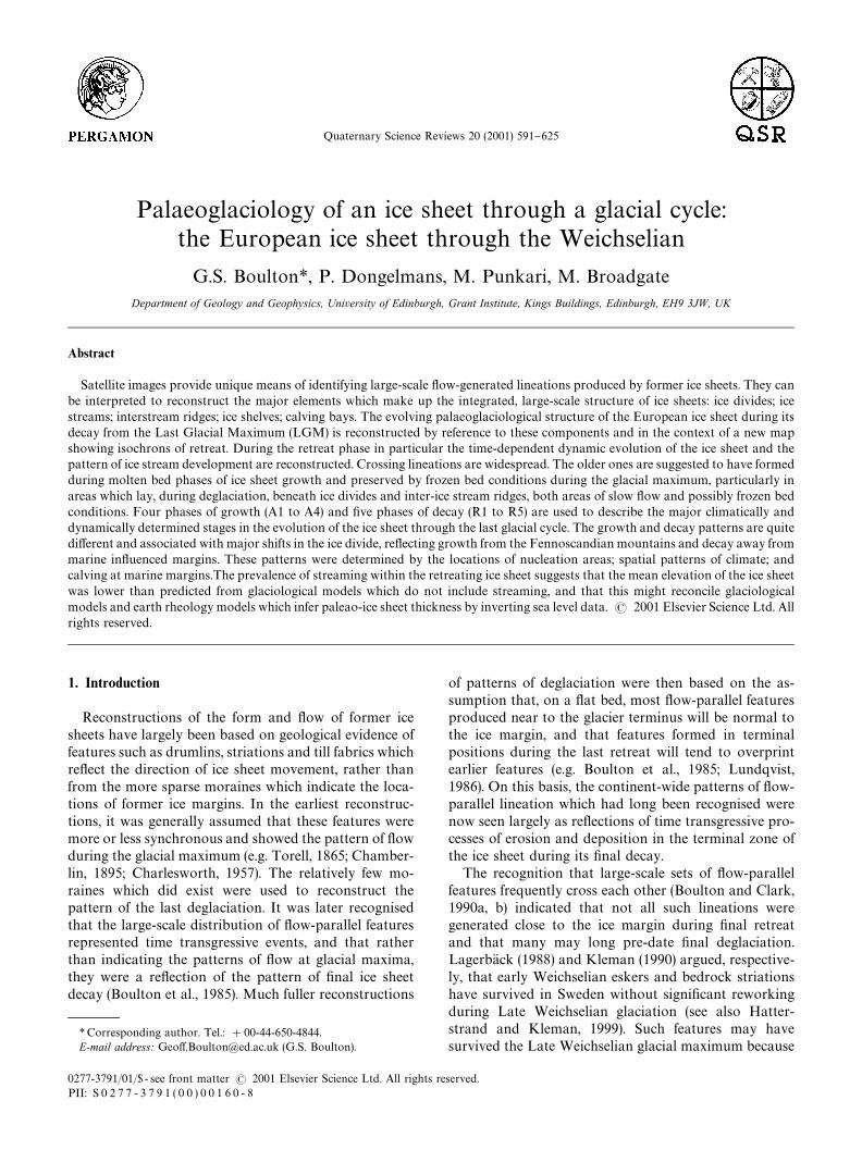
Fig. 3. Examples of interpretations of satellite images. (a), (c), and (e) show "rst-order interpretations directly from satellite images. (b), (d) and (f) showinterpretations of the pattern in terms of integrated, second-order lineation sets. Di!erent second-order sets are shown by di!erent arrow types. (a}b)Image f5 (see Fig. 1) in the area of the "rst and second Salpausselka moraines in eastern Finland. The interpretation suggests an oldest fanninglineation pattern (possibly an ice stream) re#ecting a NNE}SSW #ow, overlain by successively younger lineations re#ecting NNW}SSE #ow. TheNNE}SSW sets south of the "rst Salpausselka moraine are separated because of the long ice sheet still-stand at the moraine. (c}d) Image f10b (Fig. 1) ineastern Finland. An older NS lineation with a superimposed NW}SE lineation. Earlier (dashed line) and younger integrated sets are distinguished. (e}f)Image f16 (Fig. 1) from northern Finland showing an early N}S lineation superimposed by an older and a younger WNW}ESE lineation, convergenttowards the SE, re#ecting a change from non-streaming #ow to streaming #ow towards the head of the White Sea during ice sheet retreat.

3. Relating geological features to palaeo-glaciology

The orientation, frequency and possible cross-cuttingrelationships of #ow-parallel lineations are the primarydata upon which palaeoglaciological inferences arebased. We discuss below how this data has been inter-preted in glaciological terms.

3.1. Evolution of time transgressive lineations alonga yowline

The operation of an ice sheet in relation to its bed andits climatic drive can be illustrated by #owline transectsthrough the ice sheet which show variation as a functionof radial distance from the ice divide to the terminus(Fig. 6). Ice sheet #ow is conditioned by:

f on the surface: mass balance and temperature;f at the base: friction at the ice/bed interface, earth rheol-

ogy, thermal conductivity of the upper lithosphere and

the geothermal heat #ux at the base of the upperlithosphere;

f for an ice sheet yowing into the sea: iceberg calving.

Simulation models of ice sheets produce solutions forcompatible combinations of mass balance, ice sheet ge-ometry, temperature and #ow (e.g. Boulton and Payne,1994). Fig. 6 shows the way in which key propertieswhich e!ect bed processes vary along a #owline. An icesheet is a gravitational #ow driven by the long-term massbalance on its surface (Fig. 6a) which produces a longitu-dinal increase of #ux from the divide to the equilibriumline and a decrease thereafter to the terminus. The massbalance velocity, a function of mass balance and icethickness, will increase outwards, and may or may notdecline from the equilibrium line to the terminus depend-ing on the mass balance/thickness relationship (Fig. 6c).As ice #ow is temperature dependent and heat is advec-ted by #ow, the temperature/#ow coupling in the body ofthe ice sheet is complex. Numerical simulations of the


Fig. 4. Third-order interpretations, generalised from second-order lineations such as those shown in Fig. 3, showing lineation patterns over the shieldarea of the ice sheet. (a) Northern Scandinavia. Particularly interesting is the lineation convergences into the head of a very strong lineation setsrunning ESE towards the White Sea, which shows divergence along the White Sea shore. (b) Southern Finland and the area around the Gulf ofFinland. Note the crossing lineations in the inter-ice stream areas and re#ecting interactions between ice streams during their lifetimes. (c) SouthernSweden, southern Norway and part of Denmark.

European ice sheet (e.g. Boulton and Payne, 1994) sug-gest that the ice/bed interface was likely to have beenfrozen at the bed in the inner zone and at the extrememargin and melting in a broad intermediate zone(Fig. 6d). Although both internal #ow and basal decolle-ment can contribute substantially to the surface velocityof a glacier, there is strong evidence (e.g. Paterson, 1994)that where the ice/bed interface is unfrozen, a large partof the surface velocity of a glacier is due to basal decolle-

ment. The velocity trends shown in Fig. 6c will thereforetend to re#ect glacier sole velocity trends in the zone ofmelting (Fig. 6d). It has been suggested (Boulton, 1996)that the large-scale pattern of erosion and depositionbeneath an ice sheet is dependent upon the distributionof basal velocity, provided that there is deH collement atthe ice/bed interface. If the temperature is at the meltingpoint and water pressure at the bed is high, deH collementwill occur by sliding if the bed is lithi"ed, added to by bed


Fig. 5. Fourth-order longitudinal lineation sets plotted on a European scale. Note the areas of abundant crossing lineations between the stronglylineated zones which we interprete as ice streams, particularly clearly seen in southern Finland (see also Fig. 4b). They re#ect the location of sluggishinter-stream ridges. They may also be characterised by basal freezing. Crossing lineations also occur in former ice divide areas on the eastern side of theScandinavian mountain chain.

deformation if it is unlithi"ed. If the basal boundary isfrozen, it is assumed that there will be no basal deH colle-ment and no geomorphological work achieved througherosion and deposition. The large-scale pattern of ero-sion and deposition (Fig. 6f ) will depend upon the distri-bution of velocity and thermal regime.

We therefore make two initial assumptions:

f that the rate at which geomorphological work is done(erosion and deposition) will increase from the ice

divide zone, where #ow is sluggish and where the bedmay be frozen, to the outer zone of the ice sheet where#ow velocities are high (Boulton, 1996);

f that the net magnitude of the geomorphological im-pact in an area is determined by rates of erosion anddeposition integrated over the residence time of the icesheet in the area.

If the character of the bed is constant, and if the bed iseverywhere at the melting point, we would expect at


Fig. 6. Schematic diagram showing typical properties along a #ow linefor a land-based ice sheet in mid-latitudes. Typical #ow line length is oforder 103 km. (a) Ice sheet surface and bed pro"les, the bed is isostati-cally de#ected beneath the ice mass. (b) Horizontal distribution ofannual mass balance. (c) Mass balance velocity of the ice sheet . (d)Basal temperature: note that the temperature in the zone of melting isbelow 03C and increases outwards because of pressure dependence ofthe melting point. (e) Melting rate: note the tendency towards freezingat the extreme ice sheet margin. (f) This shows the pattern of rates oferosion and deposition beneath an ice sheet expected in the Boulton(1996) theory where the ice velocity varies as shown in (c).

a given site overidden by the glacier:

f a short period of rapid geomorphological changewhilst the site lies in the terminal zone;

f as the glacier expands further, the site will be overlainby progressivelt more slowly moving ice and be subjectto progressively slower rates of geomorphologicalchange for long periods (Fig. 7a).

At sites far from the margin, which are subject tolong-term glacier occupancy, we would expect the linea-tion pattern to re#ect long-term patterns of #ow, exceptwhere ice divides have shifted strongly (e.g. Boulton andClark, 1990a, b) or where an earlier unfrozen bed hadbecome frozen (e.g. Kleman, 1990).

In a growing glacier, we expect the inner zone offreezing to expand, inhibiting geomorphological activity

in a progressively wider inner zone of the ice sheet,producing younger landscapes and sediments in theouter, unfrozen zone whilst inner zones are progressivelyfrozen (Fig. 7, A1}A6). At the glacial maximum, thesubglacial landscape will be made up of a largely isoch-ronous surface in the outer melting zone (Fig. 7, A6) anda strongly time transgressive surface, in which landscapesand sediments become younger in distal sequence, in theinner frozen zone (A1}A6).

During ice sheet retreat (Fig. 7b), the marginal zone offast landscape formation will be the last to which a givenarea is subject. As a consequence, lineations will tend tore#ect near-margin #ow directions to a greater extentthan during advance, and the surface will be time trans-gressive, with phases R1}R6 represented in proximalsequence. If the ice sheet retreats at a constant rate, #owvelocities in the outer zone will progressively diminish inthe later stages of retreat, as will lineation intensity,thereby making it more likely that old lineations cansurvive in the central area of the ice sheet. If the rate ofretreat is slow or zero, the area which was at the marginduring that phase will tend to show stronger, more stablelineations than elsewhere.

3.2. Patterns of areal variation

Ice sheets also show well-de"ned areal patterns of#ow which de"ne major structural elements which wesuggest can be palaeoglaciologically identi"ed fromlarge-scale patterns of orientation and frequency of#ow lineations (Fig. 8). We describe below the patternsof lineation which would be expected to occur inassociation with important structural elements of icesheets. These are used in Section 4 as a key to infer someof the evolving characteristics of the ice sheet during itsretreat.

3.2.1. Ice dividesIce divides are lines of #ow divergence. They provide

the framework within which the #ow system operates.Their location is a consequence of patterns of accumula-tion on the ice sheet surface and patterns of ice draw-down in areas of fast #ow. Horizontal #ow rates are lowin the vicinity of divide ridges. The ice divides can besubdivided as follows (Reeh, 1982; Boulton and Clark,1990):

f principal (1st order) divide ridges which occur at thehighest point of an ice sheet with ice #owing away onboth sides at right angles. These ridges tend to beapproximately horizontal.

f subsidiary ridges which lead away from principal di-vides and form a hierarchy of 2nd and 3rd order ridges,etc. These ridges are inclined away from the principaldivides. Flow diverges from lower-order ridges at in-creasingly acute angles.


Fig. 7. Patterns of time-transgressive landform formation during ice sheet advance and retreat phases. Above the horizontal lines are shown successiveice sheet pro"les. Below the lines are plotted the rate of landform formation by patterns of erosion and deposition such as shown in Fig. 6f. Continuouslines show isochrons of landform formation. (a) During advance, although the greatest rates of landform creation will occur beneath the margin, theywill be further moulded in progressively more proximal locations as the ice sheet advances. An inner zone of freezing, which expands during ice sheetgrowth, will progressively suppress erosion and deposition, so that at the maximum of glaciation, there will be a time transgressive surface in an innerzone of basal freezing where former surfaces are preserved. Beyond this, at the glacial maximum, the surface will be isochronous. (b) During retreat,landform creation rates will also be greatest near to the margin, but will not be subject to further remoulding as it is exposed beyond the retreating icesheet. Landforms produced during retreat will therefore be strongly time-transgressive compared with those produced during advance, except for inthe inner zone of freezing. These contrasts also suggest, for instance, that fan forms generated by ice streams (see Fig. 9) may be more readily preservedduring retreat.

f triple junctions which occur where principal dividesseparate at ridge culminations, or where lower andhigher order ridges meet.

The locations of former ice divides can be approxim-ately inferred from the pattern of integrated, ice sheetwide contemporary lineations. Although we have arguedthat the dominant lineations are produced in near mar-ginal positions, so that inferences about divide locationsare hazardous, we go on to show how, in areas of cross-ing lineations, the contrasts between the orientiations ofolder and younger lineation sets can yield importantinferences about shifts in ice divides.

3.2.2. Ice streamsIce streams on modern ice sheets are relatively narrow,

fast-#owing longitudinal zones 10}100km in width andseparated by low-velocity zones. Flow velocities in icestreams are typically an order of magnitude larger thanin inter-stream zones. They occur between low-orderdivide ridges (typically 3rd}4th order divides), receiving#ow from wide fringing areas and discharging the #uxfrom large, ice divide-bounded glacier basins. Antarcticice streams tend to discharge into ice shelves and tomaintain a velocity increase up to their margins becausethey lie entirely in accumulation areas and bed friction isreduced as they move into the marine environment. As


Fig. 8. A cartoon showing the structure of an ice sheet. It shows form lines on the surface, "rst-, second- and third-order #ow divides, ice streams,inter-stream ridges, ice shelves and calving bays. The divide between the ice streams at the bottom of the diagram is of third order. The locations ofdivides may be controlled by the distribution of accumulation or because of drawdown by #anking ice streams, calving bays and ice shelves. Thediameter of the ice sheet is presumed to be of order 103km.

a consequence, they show little tendency to fan out intheir terminal zones. There are currently no examples ofanalogous land-based ice streams, but the piedmontlobes of the southern Alaskan glaciers, such as the Malas-pina, may be thought of as models for terrestrial icestream terminations. They fan out strongly in their ter-minal zones on the coastal plain. A terrestrial ice stream,con"ned between ice rather than rock walls, will alsotend to fan out at its margin and extend further than the#anking ice because of the faster #ow along it. We there-fore expect ice streams in former ice sheets which termin-ated on land to be recognised by patterns of strongdivergence of #ow-lineations in their terminal zones (Fig.8). The beds of ice streams are believed to be always at themelting point (Shabtaie et al., 1987). Some have beenshown to be underlain by soft sediments which wereprobably deforming (Alley et al., 1987; Kamb and Engel-hardt, 1989). Although some lie above subglacial troughs,their margins are not usually correlated with subglacialtrough boundaries (Shabtaie and Bentley, 1987). Therelatively low frictional resistance at the bed suggests that

most shear strain within them occurs at the bed. Thestrong drawdown which they produce will in#uence theevolution of ice divides, whose location, in turn, deter-mines the ice #ux available to feed the ice stream.

The velocity contrast between an ice stream and the#anking zones (Hughes, 1981) suggests that the rate atwhich sedimentological and geomorphological work willbe done along them is much greater than in #ankingzones. Moreover, fast ice streams have broad catchmentareas from which large #uxes are discharged to the icesheet margin by a relatively narrow stream. We mighttherefore expect such zones of fast #ow to have a con-siderable e!ect for hundreds of kilometres from the icesheet margin, and to be able to overprint older lineationsfar from the margin. Longitudinal zones of strong linea-tion which contrast with #anking zones of weaker linea-tion, and the preservation of old lineations beneath these#anking zones, are therefore taken to be strong evidencefor former ice streams.

During much of the "nal retreat of the European icesheet, the eastern sector of the ice sheet either terminated


Fig. 9. Interpretation of ice stream generated lineations. (a) Form ofa typical Antarctic ice stream #owing directly into a deep sea area. Ithas a wide proximal catchment areas and inter-stream ridges. It tendsto #ow into the sea without fanning in the termimal zone, except whereit #ows into an ice shelf. There is basal melting in ice streams andfreezing tends to occur beneath inter-stream ridges. Velocities continueto increase to the terminus. (b) Postulated form of an ice streamterminating on land or in very shallow water. The absence of a majorcalving margin results in a decrease in velocity towards the margintogether with longitudinal compression, fanning out of the #ow andlobation of the margin near to the terminus. (c) Schematic diagramshowing a time slices of a retreating ice sheet margin subject to stream-ing and the #ow patterns associated with it. Streaming occurs betweentime slices A to E, and produces strong lineation on the bed because ofhigh velocities. Lobation of the margin is produced in the high-velocityzone, which produces, as a result of retreat, a series of overlappinglineations. Streaming ceases between time slices E and F. Margin F isnot therefore lobate and there is no marginal fanning of lineations. Thecontinuation of strong lineations on the bed up-glacier of marginF re#ects the up-glacier extent of strong streaming during the "nalstages of ice stream existence, and can be used to estimate the length ofthe ice stream during these "nal stages. Note that the width of the icestream up-glacier of the marginal zone of fanning is much less than thewidth of the terminal lobe.

on land or in glacier-isostatically raised sea levels of nomore than a few tens of metres. Given the contrastbetween this and the depths of water in which Antarcticice streams terminate (800}1000m in the Ross Sea em-bayment in Antarctica, for example), we characterise theice streams on the eastern margin of the European icesheet as terrestrial. The lineation geometry to be expectedfrom terrestrial ice streams is shown in Fig. 9 (see alsoFigs. 3a, b, e, f, 4 and 5). The apparent (transverse) widthof the stream re#ects time transgressive movement of thelobate margin. The up-glacier width of the stream is verymuch less. Cessation of streaming activity should bere#ected by lobe collapse, straightening of the ice sheetmargin and narrowing of the apparent width of thestream. The up-glacier distance from the point at whichthis occurs gives an index of the length of the fast icestream and of ice stream width immediately beforestreaming ceased. Fig. 9 illustrates the way in whichcareful analysis can discriminate time transgressive fromcontemporaneous spatial patterns. Very short lived lobesmay be an expression of surging.

3.2.3. Inter-stream ridgesThese are usually triangular or ellipsoidal areas of

slow-#owing ice between ice streams. They may be frozenor at the melting point (Shabtaie et al., 1987). In Antarc-tica, ridges are characterised by ice #ow rates whichare 1}2 orders of magnitude lower than those foundin adjacent streams (Shabtaie et al., 1987; Stephensonand Bindschadler, 1990). Zones between palaeo-icestreams often show complex patterns of crossing linea-tions, which we interpret as including older, relictlineations preserved because of low #ow velocities inthe inter-ice stream zone. In some cases, there appear tobe no #ow lineations which re#ect the general directionof ice #ow contemporary with the ice streams, in whichcase we conclude that bed freezing inhibited lineationformation.

3.2.4. Basal freezing in divide areasNumerical simulations of mid-latitude ice sheets tend

to show a frozen ice/bed interface in the ice divide zone(e.g. Boulton and Payne, 1994) where we would notexpect signi"cant geomorphological work to be done.Kleman (1992) has shown how strong contrasts in theorientation of #ow lineations observed in "eld surveysbetween adjacent zones can be interpreted as re#ectionsof former interfaces between frozen and unfrozen basalzones. We observe the preservation of old lineations informer divide zones on satellite images (see Fig. 4a),which can be interpreted as preservation of old featuresat a frozen ice/bed interface.

3.2.5. Ice shelvesIce shelves are thick sheets of #oating ice that are

generally about 200}300m thick at their termini and up

to 1 km thick at the grounding line. They survive highrates of iceberg calving at their termini because of high#ux rates of ice into their proximal zones, which tend tobe delivered by ice streams (e.g. Hughes, 1982) depending


on the shape of the basin and the #ux from feeder icestreams. For stability, an extensive ice shelf is believed torequire a marine embayment, preferably with islandswhich block outward #ow or subshelf grounding points(van der Veen, 1986). Although palaeo-ice shelves prob-ably existed around the margins of the European icesheet from time to time in such places as the NorwegianChannel and in deep water embayments along the icesheet's western and northern maritime margins, there isas yet little direct geological evidence of their existence.

3.2.6. Zones of strong marine drawdownSuch e!ects occur where major embayments occur at

a marine margin of an ice sheet, such as around KogeBugt in south}east Greenland or the Amery ice shelf inAntarctica. Rates of ablation at such margins are highbecause of iceberg calving, leading to proportionatelyhigher rates of mass loss at that sector of the margincompared with un-embayed margins, whether they aremarine or not. As a consequence, ice sheet #ow is drawndown towards that sector of the margin, producing a ma-jor in#uence on regional ice sheet #ow patterns (Robin,1979). We expect to see such features re#ected in large-scale convergence of #ow lineations.

3.3. Areal variations in the frequency of lineations

We observe strong areal variations in the frequencyof #ow lineations. Some may be attributed to glaciologi-cal features such as the development of ice streams andothers appear to be related to topography and geology.

Lineation frequencies are lower in mountainous areasof western Scandinavia (Figs. 4 and 5). Here, only the#anks of valleys and, if they are wide enough, valley#oors bear signi"cant lineations. The relative absence oflineations from mountain massifs may be a consequenceof their destruction by intense, post-deglaciation perig-lacial weathering which has modi"ed glaciogenic land-forms, and #uvial erosion along narrow valley #oors. Itmay also re#ect basal freezing and/or low ice velocitiesduring ice sheet glaciation, resulting in low erosion rates.

In the shield areas, there are strong lineations causedby glacial erosion and drumlin formation. Drumlins areoften of relatively high relief and are readily mapped byground survey, from conventional aerial photographsand from topographic maps (e.g. GluK ckert, 1974). Similarground surveys in the more southerly zones of sedimen-tary rocks have failed to reveal more than a few isolateddrumlins or drumlin "elds. However, initial results ofmapping from satellite images in this zone reveal exten-sive drumlin "elds (Perry, 1998). This probably re#ectsthe existence of lower relief drumlins compared with theshield areas, the di$culty of identifying drumlins indensely farmed arable terrain and the masking of #owparallel features by more numerous transverse moraines.Contrasts between shield and non-shield drumlins may

re#ect controls on drumlin evolution due to contrasts inthe thickness of soft sediment overlying bedrock as sug-gested by Boulton (1987).

4. The last deglaciation

4.1. Geological reconstruction * the pattern of retreat

We use two types of data in reconstructing the patternof retreat. From the area of the shield we use the #owlineations and a relatively small number of ice marginalmoraines observed on satellite imagery. In the #ankingarea of younger sediments, we utilise a compilation of"eld observations from a variety of authors and a rela-tively small cover of satellite images from the Baltic statesand north west Russia and Belorussia.

Figs. 3}5 show that from the area in which satelliteimages have been used, #ow lineations from di!erentphases of ice sheet history are preserved and superim-posed. In this section, we identify those lineations whichwe suggest have been produced during the last deglaci-ation. In Section 5 we show how they can be stripped awayin order to infer ice sheet #ow patterns from earlier stages.

Ice marginal landforms (end moraines, outwash plains,etc.) produced during deglaciation are direct evidence ofthe pattern of "nal retreat (Fig. 10). However, except forthe Younger Dryas moraines, only a few signi"cant endmoraines occur in the Shield areas to guide reconstruc-tion of deglaciation. Following rules set out in Section 3,we expect that the strongest lineation to be generated inthe submarginal zone of the ice sheet where velocitieswere highest (Fig. 6), that in most cases, the greatestlineation density will re#ect #ow in this zone during theretreat phase, and that, on a horizontal bed, the trend ofthese lineations will lie normal to the trend of the icemargin. The prime exceptions to this will be:

f where fast ice streams have produced strong lineationsfar from the ice sheet margin and which are preservedbecause streaming #ow ceases prior to deglaciation ofthe area,

f where lineations are created in a zone of melting andwhich are preserved because of onset of ice/bedfreezing prior to deglaciation.

If we apply these rules to lineations in areas where icemarginal moraines have survived, we "nd that the icemarginal retreat pattern inferred from the densest linea-tions coincides with that inferred from moraines (e.g.Figs. 3a and b). This approach permits us to:

f de"ne the general pattern of retreat with much greaterprecision than by using ice margin-parallel formsalone,

f identify those lineations which are not normal to theretreating ice margin, and which thus re#ect either


Fig. 10. The principal zones of ice marginal moraines and other ice marginal deposits within the area of the Weichselian ice sheet. Apart fromthe Younger Dryas Salpausselka moraines and their correlatives, most moraines occur within the zone of rleatively slow retreat lying beyond the shield(cf. Fig. 12).

#ow patterns far from the retreating ice margin orpatterns produced prior to the "nal retreat.

In Fig. 11, following Boulton et al. (1985), we haveinferred ice margin trends during retreat by assumingthat they lie normal to the dominant #ow lineations. Thisgives a clear picture of the trajectory of retreat of the icemargin and of the submarginal #ow patterns associatedwith it. It permits us to infer aspects of the dynamicbehaviour of the ice sheet during retreat.

Beyond the Shield, in the area south of the Baltic Sea,much of the evidence of ice sheet behaviour during re-

treat comes from the distribution of major morainicridges formed at the maximum and during retreat. Themaximum extent of the ice sheet and its retreat in thenortheastern North Sea and on the Norwegian continen-tal shelf has been summarised by Holtedahl (1993) andSejrup et al. (1994).

4.2. Geological reconstruction * the tempo of retreat

In this section we attempt to translate the pattern ofretreat shown in Fig. 11 into one showing speci"c isoch-rons (Fig. 12). This is relatively simple in the Shield area


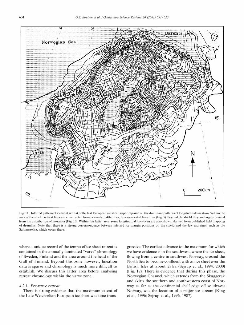
Fig. 11. Inferred pattern of ice front retreat of the last European ice sheet, superimposed on the dominant patterns of longitudinal lineation. Within thearea of the shield, retreat lines are constructed from normals to 4th order, #ow-generated lineations (Fig. 5). Beyond the shield they are largely derivedfrom the distribution of moraines (Fig. 10). Within this latter area, some longitudinal lineations are also shown, derived from published "eld mappingof drumlins. Note that there is a strong correspondence between inferred ice margin positions on the shield and the few moraines, such as theSalpausselka, which occur there.

where a unique record of the tempo of ice sheet retreat iscontained in the annually laminated `varvea chronologyof Sweden, Finland and the area around the head of theGulf of Finland. Beyond this zone however, lineationdata is sparse and chronology is much more di$cult toestablish. We discuss this latter area before analysingretreat chronology within the varve zone.

4.2.1. Pre-varve retreatThere is strong evidence that the maximum extent of

the Late Weichselian European ice sheet was time trans-

gressive. The earliest advance to the maximum for whichwe have evidence is in the southwest, where the ice sheet,#owing from a centre in southwest Norway, crossed theNorth Sea to become con#uent with an ice sheet over theBritish Isles at about 28 ka (Sejrup et al., 1994, 2000)(Fig. 12). There is evidence that during this phase, theNorwegian Channel, which extends from the Skaggerakand skirts the southern and southwestern coast of Nor-way as far as the continental shelf edge o! southwestNorway, was the location of a major ice stream (Kinget al., 1996; Sejrup et al., 1996, 1987).


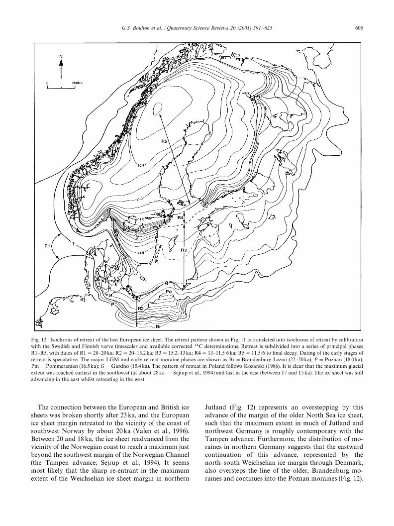
Fig. 12. Isochrons of retreat of the last European ice sheet. The retreat pattern shown in Fig. 11 is translated into isochrons of retreat by calibrationwith the Swedish and Finnish varve timescales and available corrected 14C determinations. Retreat is subdivided into a series of principal phasesR1}R5, with dates of R1"28}20ka; R2"20}15.2ka; R3"15.2}13 ka; R4"13}11.5 6 ka; R5"11.5/6 to "nal decay. Dating of the early stages ofretreat is speculative. The major LGM and early retreat moraine phases are shown as Br"Brandenburg-Lezno (22}20ka); P"Poznan (18.0 ka);Pm"Pommeranian (16.5 ka); G"Gardno (15.4 ka). The pattern of retreat in Poland follows Kozarski (1986). It is clear that the maximum glacialextent was reached earliest in the southwest (at about 28ka* Sejtup et al., 1994) and last in the east (between 17 and 15 ka). The ice sheet was stilladvancing in the east whilst retreating in the west.

The connection between the European and British icesheets was broken shortly after 23 ka, and the Europeanice sheet margin retreated to the vicinity of the coast ofsouthwest Norway by about 20 ka (Valen et al., 1996).Between 20 and 18ka, the ice sheet readvanced from thevicinity of the Norwegian coast to reach a maximum justbeyond the southwest margin of the Norwegian Channel(the Tampen advance; Sejrup et al., 1994). It seemsmost likely that the sharp re-entrant in the maximumextent of the Weichselian ice sheet margin in northern

Jutland (Fig. 12) represents an overstepping by thisadvance of the margin of the older North Sea ice sheet,such that the maximum extent in much of Jutland andnorthwest Germany is roughly contemporary with theTampen advance. Furthermore, the distribution of mo-raines in northern Germany suggests that the eastwardcontinuation of this advance, represented by thenorth}south Weichselian ice margin through Denmark,also oversteps the line of the older, Brandenburg mo-raines and continues into the Poznan moraines (Fig. 12).


The con"guration of moraines in northern Germanyand Poland (Fig. 12) suggests that an early advanceoccurred in this sector to the glacial maximum along theBrandenburg}Lezno moraines, and that this was fol-lowed by a retreat and then a readvance which createdthe Poznan stage moraines (Kozarski, 1986, 1988). Fur-ther to the east and west, the readvance formed theglacial maximum. It is possible that the early, Branden-burg}Lezno advance was a consequence of stronger icesheet #ow down the axis of the southern Baltic Sea. Itmay re#ect the same phase of ice sheet growth which ledto extension of ice from the southern Norwegian centre ofice sheet growth into the North Sea.)

The later, Pommeranian moraines (Fig. 12), have beenshown by Kozarski (1986) to cut across the earlier, post-Poznan moraines in Poland, representing yet anothermajor advance of the ice sheet margin in this sector. TheGardno moraine in northernmost Poland (Kozarski,1986) may represent a relatively small readvance, as thereis no clear evidence of major cross-cutting relationshipswith the major moraines to the south.

There is very little independent evidence of the age ofthe glacial maximum or of ice marginal positions in thesouthern (German}Polish) sector of the ice sheet. Priorto its maximum extent, the expanding ice sheet movedacross the southern Norwegian and southwest Swedishcoasts between 30 and 24 ka (Hillefors, 1974; Andersen,1987) and crossed the Polish coast slightly before 22 kaBP (Kozarski, 1988). The ice sheet is suggested to haveadvanced to the maximum extent in Poland shortly after20ka BP (TL yr * Ralska-Jasiewiczowa and Rzet-kowska, 1987; Mojski, 1992). The time window for theglacial maximum in Poland is closed by an uncalibrated14C date of 13,500 BP on the northern coast of Polandon the earliest organic deposits after deglaciation(Ralska-Jasiewiczowa and Rzetkowska, 1987). Adjustingthis date using the correction of Bard et al. (1993), givesan age of 15,950 BP (from here on 14C ages are given ascorrected ages unless otherwise stated). Although there isconsiderable uncertainty about the timing of the glacialmaximum and of deglaciation of the area to the south ofthe Baltic Sea, the above estimates are not inconsistentwith other records. The isotopic minimum in deep oceanstratigraphy, thought to record the global ice volumemaximum during the last glacial period, occurred at22ka (Imbrie et al., 1984) as did the period of maximumcooling in the Greenland ice core record (Johnsen et al.,1992; Bond et al., 1993).

Support for the general distribution of retreat isoch-rons in the southeast sector of the ice sheet during theearly stages of retreat is given by Sandgren et al. (1997),who have used palaeomagnetic correlations withvarve dated sites in southern Sweden and Kareliato suggest deglaciation of Lake Tamula in Estoniaat 14,400 calendar years BP. It indicates that theproposed isochrons are consistent with the time of de-

glaciation of northern Poland and of southern Estonia(Fig. 12).

If the ice sheet readvances in the southern sector mar-gin (Kozarski, 1988) are climatically driven rather thandynamic it is tempting to suggest the following correla-tions with post LGM cooling events in the GISP/GRIPrecords: Poznan moraine * 18,500 BP; Pommeranianmoraine * 16,500 BP; Gardno moraine * 15,400 BP;compared with Kozarski's (1986) estimates of 20,400for the Lezno, 18,400 for the Poznan, 15,200 for thePommeranian and 13,300 BP for the Gardno moraines.

The trend of morainic features in the southeasternsector of the ice sheet suggests that the features which areco-linear with the Gardno moraine ultimately converge,about 300km south of Lake Ladoga, with the maximumextent of Weichselian glaciation (Fig. 12), just as thePoznan and Pommeranian moraines appear to furtherwest. If this is so, it suggests that whilst the southern andsouthwestern margins of the ice sheet were retreating byup to 300km, the eastern and southeastern margins ofthe ice sheet were stationary or still advancing. Thisconclusion is supported by evidence that in the area tothe southeast of the White Sea, the glacial maximum wasnot reached until after 17 ka and that retreat from themaximum position did not commence until about 15 ka(Larsen et al., 1999).

In the northern sector, the ice sheet appears to havereached a maximum in northern Norway between19}18.5ka BP (Vorren et al., 1988), whilst an ice sheetover the Barents Sea, believed to have been con#uentwith the European ice sheet, is thought to have reachedits maximum extent and begun to collapse rapidly by15ka and had largely disappeared by 12 ka (Landviket al., 1998).

4.2.2. The varve zoneThe most important record of the tempo of deglaci-

ation lies in the varve-based `Swedish Timescalea (DeGeer, 1940), which has been extended back continouslyfrom "nal deglaciation at about 8,700 varve years BP toabout 11,500 varve years BP (StroK mberg, 1985).However, Younger Dryas advances of the ice sheet inthe Middle Swedish end moraine zone make it verydi$cult to connect this chronology with that representedby about 2000 varve years in southern Sweden. Thelatter is a #oating chronology because of dislocationin the Middle Swedish end moraine zone, but if thisdislocation is ignored, appears to extend back to about13,300 varve years BP (e.g. Wohlfarth et al., 1995;StroK mberg, 1994; BjoK rck, et al., 1995). The workof StroK mberg (1994) appears to indicate that themaximum of the Younger Dryas readvance in the MiddleSwedish zone was reached at 11,410 varve years BP,and that ice front positions occupied during a periodof 180 yr were later overridden by the Younger Dryasreadvance.


The interpretation summarised by BjoK rck, et al. (1995)and Wohlfarth et al. (1995) (also Wohlfarth personalcommunication, 1995) can in principle be used to inferthe rate of ice sheet retreat from 13,258 varve years BP, ineastern Scania, to 9200 varve years BP in VaK sternorr-land. Although correlation between varve and 14C yearshas been di$cult to achieve, a direct comparison of varveand AMS 14C chronology (BjoK rck et al., 1995) shows thelatter to be systematically older by 500}1500 yr duringthe period 9500}12,500 varve years BP, although there isgood agreement between the varve chronology and the14C chronology calibrated (Stuiver and Reimer, 1993)against the German oak-pine chronology (Kromer andBecker, 1993) and U/Th ages on corals (Bard et al., 1993)up to about 12,000 varve years BP. The U/Th-calibrated14C record beyond 12,000 varve years BP gives muchgreater ages than the varve record.

A means of con"rming the precise magnitude of themis-match between varve years and calendar years beforepresent has been developed by Andren et al. (1999). Theyhave suggested that varve thickness will largely re#ect icesheet melting rate as a direct result of changing summertemperatures. They have then compared varve thicknessdata for the period 10,250}11,550 varve years with theGRIP ice core 18O record (Johnsen et al., 1992), which isprobably the best proxy, high resolution guide to thetrend of climatic variations in western Europe during theperiod, re#ected for example in the excellent match be-tween the GRIP record (Fig. 13a) and the sea surfacetemperatures in the North Atlantic (Fig. 13b; Kroonet al., 1997). They show that a very good correlationexists between the two records for the highly distinctivepattern of change during the Younger Dryas/Preborealclimatic shift, provided that 875 yr are added to the varveages.

We have therefore added 875 yr to the whole varvechronology, and added 180 yr to that part lying south ofthe Middle Swedish end moraines, to produce the patternof ice sheet retreat rate shown in Fig. 13c. The pattern isvery similar to that shown by the GRIP and NE Atlanticrecords, but lags behind it. The best "t is obtained byassuming that the retreat rate lags 250}500 yr behindphases of climatic warming. This is discussed further inSection 4.4.

This corrected varve based chronology is now appliedto the ice sheet retreat pattern shown in Fig. 11 byascribing ages to retreat isochrons at the points at whichthey cross the varve transect series in eastern Sweden.Fig. 14a shows the inferred pattern of time-dependentretreat of the southern sector of the ice sheet, not onlyfor the area to which the corrected varve timescalecan be applied, but also for the earlier phase of retreatby using the tentative correlations o!ered between Poz-nan, Pommeranian and Gardno readvances andKozarski's (1986, 1988) estimate of retreat rate betweenthem.

A varve chronology for Finland was "rst published bySauramo (1918), but has been a `#oating chronologyauntil recently. StroK mberg (1990) has suggested that thezero varve of the Finnish chronogy (Sauramo, 1923) wasequivalent to 10,643 varve years in the Swedish chrono-logy. We have used this as the basis of our chronology inFinland. It has now been extended to the area of theeastern Gulf of Finland and as far as Lake Ladoga(Hang, 1997).

Although it is still premature to create an unequivocalreconstruction of European ice sheet deglaciation in viewof much poor or heterogeneous dating evidence, theabsence of evidence of ice margin trends in sea areas,and the fragmentary evidence of trends in areas such asBelorussia, it is helpful to create a deglaciationhypothesis as a spur to testing and to provide a bestestimate of deglaciation for quantitive simulationmodels. We argue that evidence of trends of ice marginsand the varve chronology in much of Sweden, and toa lesser extent in Finland, make it possible to producea persuasive reconstruction of deglaciation in thoseareas. South of the Baltic and the Gulf of Finland andin northern Finland and the Kola peninsula, thedating evidence is sparse, and ice marginal trendsare uncertain east and southeast of the Gulf of Finland.However, we have combined the concentric trendsnormal to #ow lines shown in Fig. 11 with the evidenceof ice marginal landforms and the chronological informa-tion discussed above to reconstruct the tempo andpattern of ice sheet decay during the last deglaciationin Fig. 12. The inferred tempo of deglaciation alonga transect from northern Poland to western Norwaythrough the centres of "nal ice sheet decay in Norrbottenis show in Figs. 14a}c using the adjusted varve timescalebased on the correlation with GRIP by Andren et al.(1999).

4.3. Glaciological inferences * streaming within theretreating ice sheet

We have assumed that, on a relatively #at surface, verystrong #ow-parallel lineation sets and/or evidence oflobation of the ice sheet margin indicate the fomer exist-ence of an ice stream. However, lobate ice margins can beinterpreted in two ways: as the termini of ice streamswhich protrude beyond the normal ice margin because ofhigh ice velocities along their axes, or as expressions ofradial #ow from the end of an ice divide or ice dome (seeFig. 8). In the "rst case they represent a zone of relativelyfast #ow, in the second, a zone of relatively slow #ow.Lagerlund (1980) has interpreted the southern Baltic Sealobes as evidence of an ice dome in the southern Balticrather than of ice streams. Lobes and associated linea-tions which occur entirely on land, for instance in Fin-land, show lineations at their margins which are notnormal to the margins, as would occur if they were ice


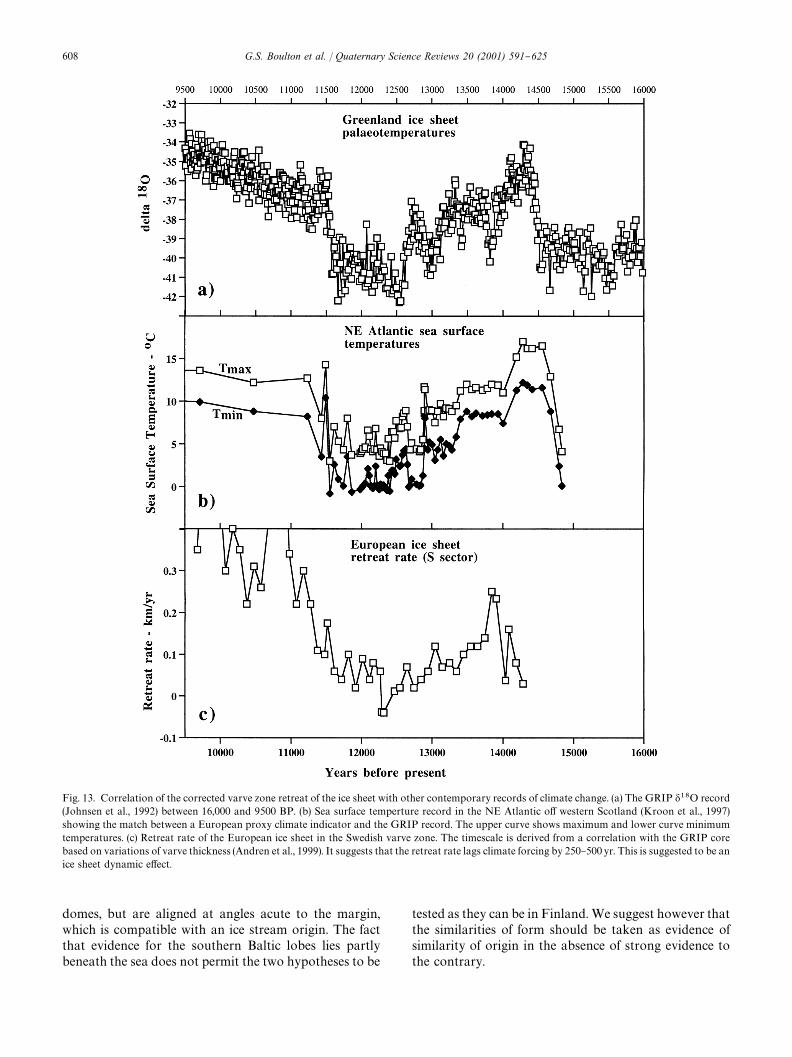
Fig. 13. Correlation of the corrected varve zone retreat of the ice sheet with other contemporary records of climate change. (a) The GRIP d18O record(Johnsen et al., 1992) between 16,000 and 9500 BP. (b) Sea surface temperture record in the NE Atlantic o! western Scotland (Kroon et al., 1997)showing the match between a European proxy climate indicator and the GRIP record. The upper curve shows maximum and lower curve minimumtemperatures. (c) Retreat rate of the European ice sheet in the Swedish varve zone. The timescale is derived from a correlation with the GRIP corebased on variations of varve thickness (Andren et al., 1999). It suggests that the retreat rate lags climate forcing by 250}500 yr. This is suggested to be anice sheet dynamic e!ect.

domes, but are aligned at angles acute to the margin,which is compatible with an ice stream origin. The factthat evidence for the southern Baltic lobes lies partlybeneath the sea does not permit the two hypotheses to be

tested as they can be in Finland. We suggest however thatthe similarities of form should be taken as evidence ofsimilarity of origin in the absence of strong evidence tothe contrary.


Fig. 14. Tempo of retreat of the ice sheet along composite A}B, B@}C in Fig. 19. (a) Retreat along the transect on the southern #ank of the ice sheet. Theearly part of the retreat is based on estimates of age by Kozarski (1986, 1988) and speculative correlations with the GRIP record. After 15.2 ka, thetempo of retreat is well controlled by the varve chronology as far as to the north of Stockholm. Beyond this point, varve dates are projected ontothe line of section using the isochron map (Fig. 12). (b) Net retreat during each of phases R2}R5 along the transect on the eastern (right) and western(left) sides of the "nal ice divide. The tempo of retreat on the western #ank of the ice sheet prior to 13 ka (Younger Dryas) is poorly known. (c) Retreatrates during phases R2}R5 on the eastern (light shading) and western (dark shading) #anks of the ice sheet. Retreat rates are invariably less on thewestern side of the divide, re#ecting less negative mass balances on the more maritime and mountainous #ank.


The relationship between lobation and strong linea-tion can be used to infer the time transgressive history ofan ice stream and to infer its length as shown in Fig. 9.Using this approach, the inferred pattern of time trans-gressive streaming in the ice sheet during its retreat isshown in Fig. 15. This diagram does not show the lengthof ice streams at any one stage of their history, but thetime periods during which ice streams reached the mar-gin of the ice sheet. It shows a lettering scheme whichidenti"es the ice streams on the terrestrial margin ofthe ice sheet. Ice streams B, F and G are deducedlargely from lobation of the contemporary ice margin.Ice stream A is suggested as a probable outcome ofthe convergence of ice #owing from #anking land areasinto the Skaggerak embayment, but there is seismic evid-ence for it from the Norwegian Channel (Sejrup et al.,2000) and lineations on Jaeren, in southwest Norway,where the ice stream transgressed onto land (Sejrup et al.,1998). Others are deduced from locally strong lineationsets.

Lineation evidence for ice streams is restricted to theeastern, northern and southern margins of the retreatingice sheet. By analogy with modern ice sheets, we wouldalso expect ice streams at the marine margins of the icesheet. Ice stream J for example, is well marked by stronglineations on land and trends distally towards a well-de"ned, over-deepened shelf trough and a lobate glacialunit, presumed to be a moraine, at the shelf edge(Roekoengen et al., 1979). In a tentative estimate of thelocations of former ice streams at the western, marinemargin, we have used over-deepened troughs on the shelfand lobate moraines or thick glacial sediment units at theshelf edge (Roekoengen et al., 1979; King et al., 1987;Roekoengen et al., 1988; Rise et al., 1988; Holtedahl,1993), as possible indicators of palaeo-ice streams, andmarked them in Fig. 15.

If we use lobation of the contemporary ice sheet mar-gin based on moraine distributions (e.g. Chebotareva,1977) as an index of streaming in the south eastern#ank of the ice sheet south of the Baltic and the Gulfof Finland, many seem to line up with streams onthe Shield which are clearly indicated by lineationspatterns. We have therefore identi"ed, using su$xes,groups as ice stream complexes which appear to recuralong the same axis and which are often succeeded bysingle major ice streams at a later stage of retreat.They are

B1 } B5 * Southern Baltic ice stream complex,E } E1 * Karelian ice stream complex,G1 } G4 * White Sea ice stream complex.

4.4. Glaciological inferences * the phases of retreat

We have characterised the structural evolution of theice sheet during its decay by subdividing it into a series ofphases as shown in Figs. 12 and 13.

4.4.1. Phase R1 * 29}20 kaThe growth of the European ice sheet culminated in its

southwest, west and northwesterly sectors during thisperiod, when it extended onto continental shelves. It thenretreated from these shelves before the GRIP core indi-cates that a signi"cant climatic warming had occurred. Itmay be a consequence of dynamic interaction betweenice sheet loading and lithosphere #exure. Boulton andPayne (1994) have shown how a shelf area which hasbecome exposed above sea level as a consequence ofglobal sea level fall may be loaded by an advancing icesheet to produce isostatic depression of the lithosphereand consequent relative sea level rise. This then enhancesthe rate of iceberg calving at the marine margin andpromotes ice sheet retreat. Such a scenario might applyto the early advance of the ice sheet from the southwestNorwegian centre of ice dispersal over the central NorthSea, where it became con#uent with the British ice sheetin a shallow sea area of average interglacial water depthof 50}70m, which would have been exposed above sealevel during a glacial maximum sea level fall of about120m (Fairbanks, 1989). Very little is known about thenature of the connection between the European andBritish ice sheets. We presume that a "rst-order ice divideextended across the North Sea from NE to SW, witha saddle at the point of con#uence.

We have referred in Section 4.2 to the evidence for anice stream along the line of the Norwegian Channelwhich was contemporary with a North Sea ice sheet.Sejrup et al. (2000) show this ice stream as a continuousfeature leading from the Skaggerak as far as the shelfedge at the maximum of glaciation. We suggest that thisis unlikely. It would have demanded a very highly asym-metric ice sheet, with an ice divide lying between theSkaggerak and the southern LGM margin of the ice sheet(Fig. 12), a mere 150 km away, but with a northwesterly#ank some 600km in extent. There are no major topo-graphic features or strong contrasts in bed materialswhich would prevent the ice divide from being locatedapproximately equidistant between the northwestern andsoutheastern margins of the North Sea ice sheet, al-though stronger draw-down at a calving margin indeeper water at the northwestern margin might havecaused some asymmetry. For this reason, we suggest thatat the maximum of glaciation, an ice stream existed in thenorthwestern area of the Norwegian Channel, drainingice from the south western fjords of Norway towards thenorthwest, and that as the ice sheet decayed, the head ofthe ice stream retreated towards the Skaggerak. It is evenpossible, given the absence of evidence of strong climaticwarming during the period, that the ice stream played animportant role in the rapid decay of the North Sea icesheet during a period of glacio-isostatic sea level rise. Thedevelopment of fast ice streams in the Norwegian Chan-nel may have drawn down the ice sheet surfaces both tothe northeast and southwest su$ciently to have created


Fig. 15. Inferred time-dependent trajectories of land-based major ice streams which existed during decay of the ice sheet, marked A}J (named in thetext). The concentric lines in each ice stream zone show the position of the ice sheet margin at times when there was streaming activity in each zone. Thearrows show the centre lines of time transgressive streams, not the length of an ice stream at any one time. Probable locations of marine ice streams areshown as M1}M10. Evidence for them comprises shelf troughs, arcuate moraines at the mouths of shelf troughs and major accumulations of glacialsediment at the shelf edge or on the upper continental slope.

a strongly negative mass balance on the ice stream #anks,leading to glacier decay and break up of the North Seacon#uence zone.

4.4.2. Phase R2 * 20}15.2 kaThis is characterized by

(a) a large net retreat in the southern sector whilst theeastern sector was stationary at, or advancing to, themaximum extent,

(b) major readvances separated by intervening retreatsof the ice sheat margin in the southwestern andsouthern sectors.

The large-scale form of the ice sheet suggests a patternof #ow re#ecting a SW}NE primary ice divide. As there isno evidence of erratic transport onto the eastern coast ofSweden from further east, Lundqvist (1974) suggestedthat the divide could never have been to the east of theSwedish east coast. However, sluggish ice velocities and


the probability of basal freezing in the divide zone makethis weak evidence. Most recent ice sheet reconstructions(e.g. Boulton and Payne, 1994)) however, place the LGMprimary divide just to the east of the SW}NE Scandina-vian mountain chain. The buttressing of the western#ank of the ice sheet by the mountain range permits thedivide to be farther west than would be the case ona horizontal bed. The ice sheet is therefore stronglyasymmetrical. As the mountain chain does not extendinto the northeast sector, we expect the divide to swinground towards the east in this sector, with second orderdivides extending north into Finnmark and east into theWhite Sea area. Strong drawdown by the Skaggerak (A)and Baltic Sea (B) ice streams can be expected to producea triple junction at the SW end of the primary divide fromwhich a second-order divide extends to the south insouthern Sweden, with a further second-order divideextending into SW Norway.

Advance continued in the east until about 15,000 BPwhilst retreat occurred further west. This is most likely tooccur as a consequence of continuing clockwise rotationof the principle ice divide as a consequence of changingpatterns of accumulation on the ice sheet surface. Thisdivide rotation is also inferred for the ice sheet build-upphase (see Section 5.2). Its most probable cause is thegeo-topographic obstruction caused by the de#ection ofatmospheric #ow by the growing ice sheet. The resultantatmospheric wave would produce a low pressure zone onthe westerly #ank of the ice sheet, drawing in warm,moist, southwesterly air. On the easterly, lee #ank of theice sheet, we would expect a dominantly high pressurezone drawing down cold, dry, polar air from the north.During colder periods, this will tend to produce highaccumulation rates on the southwestern #ank of the icesheet and low accumulation rates on the eastern #ank,producing fast growth in the west and slow growth in theeast. General climatic warming will produce retreat in thewest, whilst in the east, the more continental climate andthe existence of strong katabatic #ows, may be able tomaintain cold though dry conditions there. This contrastcould account for decay in the southwest contemporarywith continuing growth in the east.

The southern sector of the ice sheet was characterizedby lobate margins which we suggest re#ect the termini ofice streans. The sector was prone to readvance duringwhich the axes of lobes/streams changed through time.The inferred form of the ice sheet margin to the east andwest of the head of the Skaggerak suggests that it wasdrawn down by a powerful contemporary Skaggerak icestream. During the retreat of this stream into the coastalzone, and during the Pommeranian and Gardno phases,the Danish sublobe (B1) of the Baltic ice stream complexshowed very strong activity (East Jylland and Belt SeaAdvances * Lagerlund and Houmark-Nielsen, 1993)well before 14.2 ka BP. We expect shifts in the position ofterminal lobes of ice streams to re#ect changes in condi-

tions in the terminal zone rather than in the accumula-tion area. The development of a Danish sub-lobe (B1)may be a response to rapid deglaciation in the Skagerrakcalving bay. Initially, the Baltic ice stream may have beenforced to the south in the large Odra sub-lobe (B2)because of ice #owing south from Norway. Later, as theSkagerrak calving bay developed, the ice stream was nolonger blocked to the west and therefore expanded west-ward towards the Kattegat as the Danish sublobe. TheBaltic ice stream appears to have behaved as a `loose"re-hosea in the southern Baltic sector during decay.Houmark-Nielsen's (1987) reconstructions of the ad-vance of ice into Denmark immediately prior to theglacial maximum, suggest that the ice sheet may alsohave behaved in this way in the latest stages of advance.

4.4.3. Phase R3 * 15.2}13 kaThis was characterized by general retreat around the

whole of the ice sheet margin, re#ecting a strong climaticamelioration. The corrected varve record (Fig. 14a)shows a rapid early retreat followed by a deccerelationtowards the Younger Dryas moraines. Retreat at thewestern margin was much slower (Figs. 14b and c). Wesuggest that it re#ects in part a very di!erent regime ofchannelised #ows in an area of high relief, in part a con-trast between relatively heavy winter accumulation onthe west #ank of the ice sheet in contrast to more aridwinter conditions and warmer summers in the east, and,in part, strong drawdown by powerful ice streams in theeastern central sector. Particularly dramatic rates of re-treat occurred in the southern Baltic and White Searegions (Fig. 12), which we suggest were enhanced byiceberg calving.

We postulate that a contemporary ice stream at thehead of the Skagerrak (A) drew down a large part ofthe southwestern margin of the ice sheet. There are,for instance, very strong NE}SW lineation setson the northern part of the Swedish west coast whichconverge towards the head of the Skaggerak. We suggestthat both the ice stream, and a calving bay whichwe presume to have succeeded it in the re-entrant be-tween the western Swedish and southeastern Norwegiancoasts, played the dominant roles in maintaining thisre-entrant in the southwestern margin of the ice sheetduring this phase. The large-scale pattern of converging#ow which this created was re#ected in a re-entrant in theice margin for over 3000 yr after retreat from the coast-line (Fig. 12).

The extreme lobation of southeastern ice streams dur-ing phase R3 compared with their successors in laterphases, may re#ect the fact that they overlay thick poorlylithi"ed sediment sequences which facilitated subglacialsediment deformation and relatively unstable #ow condi-tions (Boulton and Jones, 1979), in contrast to the hardbasement rock surfaces to the north. This is particularlyclearly seen in the Riga (B5), Novgorod (F) and White


Sea (G) streams, whose termini become much less lobateafter about 12.5 ka.

The evidence of the earliest crossing #ow lineationsduring deglaciation comes from southern Sweden(Fig. 4c), where there is an early N}S lineation. Wesuggest that this developed during the last stages ofadvance to the Weichselian maximum or the early stagesof retreat. However, the strong drawdown by ice streamB in particular, during retreat, was responsible for thedevelopment of a second-order ice divide in southernSweden. Flow away from this divide produced lineationsets superimposed on the N}S sets which fan out towardsthe SW in west coast areas and towards the SE in eastcoast areas (Fig. 4c). We argue therefore, partly becauseof the hard rock substratum in this area, and partlybecause of the nature of the pattern, that this pattern isunlikely to re#ect activity of an ice stream, but rather thedivergence of #ow which we would expect from theformation of a subsidiary ice divide due to strong draw-down by #anking ice streams.

The distinctive warming events shown by the GRIPand NE Atlantic records at 14,000}14,500 BP and atabout 11,500}11,600 BP and the lagged response of theice sheet retreat rate discussed in Section 4.2 provide animportant index of ice sheet dynamics. The rate of retreatof an ice sheet margin re#ects the balance between thehorizontal component of ablation at the margin and thehorizontal component of velocity. If the climate becomeswarmer, we expect the ablation rate to increase (both bysurface melting and by iceberg calving) and the net massbalance on the ice sheet surface to decrease. The formerwill have an immediate e!ect, whilst a reduction in massbalance will gradually cause a reduction in velocity anda lagged retreat rate response. The lagged retreat rateresponse of about 250}500 yr to warming at14,000}14,500 BP (Fig. 13) and at about 11,500 suggeststhat the dynamic e!ect of reduced mass balance was thedominant control on retreat rate during this period,which is consistent with the fact that the ice sheet at thattime had a margin which calved into a Baltic Ice Lakeover much of its southeast sector.

4.4.4. Phase R4 * 13}11.5/11.6 kaThe Younger Dryas stadial, which occurred between

about 12,860}11,640yr BP, was associated with a suddentemperature drop of 73C at the beginning of the periodand a similar increase at the end (Johnsen et al., 1992;Bond et al., 1993). The equilibrium line altitude on the icesheet dropped by about 600}700m (Boulton et al., 1995)and was 400}600m lower than at present in the moun-tains of western Norway (Svendsen and Mangerud,1992). Large terminal moraines, the Fennoscandianmoraines, were generated in Norway (Ra moraines),Sweden (Middle-Swedish moraines) and Finland (Sal-pausselkaK I}III) with smaller moraines in RussianKarelia (Rugozero and Nyukozero moraines* Punkari,

1985), although only discontinuous moraines were pro-duced in the Kola Peninsula (Punkari, 1993). The icemargin readvanced in western Norway (Mangerud et al.,1979) and western Sweden between 12.8 and 12 ka, al-though it was either stationary or retreated slightly fur-ther east during the same time period. We presume thatthis re#ects similar west}east climatic contrasts noted inR3 (Figs. 14b}c). Varve analyses do not show major#uctuations on the southern and eastern margin ofthe ice sheet (StroK mberg, 1994). The particularly stronglineation patterns which lie to the north of the Salpaus-selkaK moraines probably re#ect a relatively stable #owpattern produced while the ice margin was approxim-ately stationary for about 1000 yr (Figs. 12 and 14).

An exception to the general pattern of little overallretreat during R4 occurs in the White Sea region, wherethere was up to 300 km of retreat (Fig. 12). Four icestreams, G1}G4, which extended across the White Sea at13.2ka were replaced by a single large ice stream, G, by12.6ka. It seems probable that G1}G4 represented di%u-ent terminal parts of a single up-glacier ice stream, andthat low basal friction on the muds of the White Seaproduced low slope lobes that stagnated and broke up bycalving. Retreat was a consequence of dynamic collapserather than of changing climate.

4.4.5. Phase R5 * 11.5/6 ka xnal retreatRapid retreat of the southeastern #ank ice sheet was

resumed and the western, southwestern and northern#anks withdrew from the marine margin more slowly asa consequence of substantial climatic amelioration.

In southwesternmost Finland, ice stream B showsa very strong splaying out in an eastward direction, butdoes not show a similar westward splay on the easterncoast of Sweden (Punkari, 1995). This appears to re#ecta failure of the Baltic Sea ice stream to #ow strongly ina southerly direction from the southern end of the Gulf ofBothnia past the islands of As land. This may have arisenbecause the southerly exit from the Gulf was blocked bya shallow bedrock sill around the As land islands, in con-trast to the soft sediment basins to north and south(Freden, 1994), so that #ow was de#ected towards thesoutheast. There is a discontinuity between the lineationsof ice stream B to the north of the SalpausselkaK morainescompared with those immediately to the south, whichhave more of a north}south trend (Figs. 15 and 16),suggesting that strong de#ection of ice stream B to thesoutheast occurred during the Younger Dryas stadial.

The lineations sets of ice stream D however, appear tocontinue beyond the SalpausselkaK moraines (Figs. 15 and16) although they show less sign of fanning south of themoraines, suggesting that the general #ow direction re-mained the same in this sector and that ice stream D wasinitiated or strengthened during the Younger Dryas sta-dial. The same is also true of ice streams E andG. Fanning out of ice stream termini during the Younger


Fig. 16. Youngest lineation sets and inferred ice margin trends during the last deglaciation of southwest Finland, with ice margin isochrons inferred byextrapolation of the adjusted Swedish varve chronology. Fig. 9c shows the key to interpretation. Two well de"ned ice streams (B and D) are present atabout 12,600 BP, joined by stream E by 11,400 at the latest. At about 11,300 BP, a new ice stream (C) forms between B and D. Streaming ceases in D byabout by about 100 yr later (11,200 BP), probably as a consequence the capture of its catchment by the new ice stream C. Ice stream C, however, hasa short life of about 200yr, appearing to lose activity by about 10,900 BP.

Dryas was generally greater than previously (Fig. 15). Itcontinued during subsequent retreat for a further 200km.We suggest that this re#ects stronger velocity contrastsbetween ice streams and inter-stream ridges and theintensi"cation of #ow during the Younger Dryas.

There is evidence in Finland of ice streams which ceaseto function and are replaced by others. This occurs whereevidence of terminal lobation ceases in an upstream di-rection (Fig. 16). The marginal lobation of ice streamD ceases after about 11.2 ka suggesting cessation ofstreaming. The strong parallel lineations which occur inice stream D up-glacier of this isochron re#ect the head-ward extent of strong streaming prior to cessation of

streaming. This appears to extend as far as the easternshore of the Gulf of Bothnia and possibly just as far as thewestern shore, suggesting that the length of the ice streamas it died at 11.2 ka was between 250 and 400km.

A major new set of fanning lineations appears betweenice streams B and D (Fig. 16) some 150km north of theSalpausselka moraine, related to an ice margin at about11.3ka. This appears to mark the birth of a new icestream, ice stream C. It appears to have grown at theexpense of ice streams D and B. Stream D "nally diedsome 100 yr later, at 11.2 ka. It also appears that icestream E grew at the expense of ice stream D. Lobation ofthe margin of ice stream C had however ceased by about


10.9ka, suggesting that it had a life of about 400 yr.Strong lineations along the axis of this ice stream appearto extend across the Gulf of Bothnia, as far as250}300km north of the 10.9 ka isochron, suggesting thatstrong streaming occured in stream C for 250}300kmfrom the ice sheet margin just prior to its decay. A similarargument applied to ice stream G gives a length of250 km. These examples illustrate how the length of thelineation sets associated with streaming re#ects timetransgressive behaviour and is not in itself a good guideto ice stream length.

The ice divide system in the Younger Dryas ice sheetcan be reconstructed to some extent. It is reasonablyclear that the major ice divide system was approximatelysigmoidal in plan, stretching from southwest Norway tonorthern Sweden and into the Kola Peninsula, wherethere was a second-order divide as a consequence ofmarine drawdown in the #anking areas of the southernBarents Sea and the White Sea (due to collapse of the icestream complex G1}G4); and in southern Sweden, be-cause of drawdown into the embayment to the west andinto the Baltic sea ice streams to the east. A series oflower-order divides existed between the southeasterly icestreams, with a more complex pattern in northwesternNorway because of the interaction between ice sheetform and the mountain topography.

After 10.6 ka, the ice sheet broke up into sepa-rate domes, the main ice mass centred to the east ofthe modern ice cap of Svartisen, along theNorwegian}Swedish border, a dome centred over theJotunheimen area in southwest Norway, and a smalldome separating later in central Norway/Sweden (JaKmt-land). The last ice caps were located farther to the eastthan the initial growth centres. Some strong lineationsentering into the northern extremity of the Gulf of Both-nia from the northwest (Fig. 4a) suggest that somestreaming continued here at least into the early part ofthis phase, although it is not clear whether this belongs toa successor of streams E, D or C, or a newly createdstream.

5. Older 6ow sets * the pattern of ice sheet growth

5.1. The pattern of pre-retreat lineations

Crossing lineations have been observed in many areas,where #ow-parallel lineations on satellite images anddrumlins and striations observed on the ground clearlypredate the #ow features produced near to the retreatingice margin during "nal deglaciation (e.g. Figs. 3}5).Superimposed drumlins re#ecting di!erent #ow direc-tions were "rst identi"ed by Rose and Letzer (1977).Boulton (1987) showed how they could be produced bychanging ice sheet #ow directions, and Boulton andClark (1990a, b) mapped crossing lineations which re#ect

such features over wide areas of Canada from satelliteimagery. In Fig. 17, all lineations which lie parallel to the#ow during "nal retreat have been removed from thetotal lineation population to reveal lineations which un-equivocally pre-date "nal retreat. This is not to say thatmany lineations which happen to be parallel to marginal#ow during "nal retreat do not pre-date that retreat,merely that our conservative approach does not recog-nise them. The residuals come predominantly from theareas of crossing lineations shown in Figs. 4 and 5. Theytend to form well-de"ned clusters, which are particularlystrong in northern Fennoscandia, although residualsoccur throughout central and southern Sweden, inparticular in southwestern Sweden. In northernFinland/Sweden and in central Sweden (Fig. 17), theseearly lineations tend to form two sets, with the earlier setin the more northerly area oriented NW}SE and the laterset oriented NNW}SSE. We suggest that many residuallineations were protected from overprinting by the re-organisation of ice sheet dynamics during the latest phaseof glaciation, by temporary phases of basal freezing (Kle-man, 1990), migration of the ice divide over the site(Boulton and Clark, 1990) or because they lay beneathzones of sluggish #ow between ice streams when the areawas in the near-terminal zone during deglaciation(Figs. 4b and 16).

The pattern of residual lineations shown in Fig. 17could have formed far from the ice sheet margin duringthe "nal retreat, or during an earlier stage of ice sheetretreat or advance, either in the Weichselian or during anearlier glacial stage (Tanner, 1915; Punkari, 1985; Nor-dkalott Project, 1986).

In southwestern Sweden, the residuals showa north}south trend compared with the NE}SW trendduring deglaciation. In central Sweden they showa NW}SE trend compared with a NNW}SSE trendduring deglaciation. In northeastern Sweden, northernFinland and northwestern Russia they show a NW}SEto NNW}SSE trend compared to a dominant W}E trendduring deglaciation; and in southern Finland they showa N}S trend compared with a NW}SE trend duringdeglaciation. In the area north of the Gulf of Bothnia, thepattern of residuals is more complex, progressivelyswinging round towards a north}south trend further tothe south and east (Fig. 17). Studies of their interrelationssuggest that the NW}SE lineation is the earlier, over-printed by a later lineation which fans out from northern-most Sweden in an arc from SW and W.

The pattern of "nal retreat on the SE #ank of the icesheet east of the Baltic Sea, with a margin oriented ina NE}SW direction, indicates that the dominant #owduring retreat in this sector was NW}SE, from a prin-ciple ice divide oriented SW}NE. We conclude thereforethat neither the N}S orientation in southern Finland, northe earlier NW}SE lineations in northeastern Swedenbelong to the "nal decay phase. However, in the Gulf of


Fig. 17. The major pre-maximum lineation sets which di!er in orientation from the retreat sets. They tend to be preserved in areas which lay beneath theprincipal ice divide at the maximum of glaciation, which protected them from erosion because of frozen bed conditions (Fig. 18) and low ice velocities(Fig. 6c), and beneath inter-stream ridges (see Figs. 5, 11 and 15) characterised by low ice velocities and possibly frozen bed conditions. Inference of basalthermal reuime: The solid lines identify di!erent lineation zones, and are explained by reference to the time-dependent thermal zonation shown in Fig. 18.Zone I: no major pre-maximum lineation sets; explained as the area in which there was no basal melting through much of the glacial cycle. Zone II: a singlemajor set of pre-maximum lineations; explained as a zone in which there was basal melting during the early Weichselian prior to 80 ka, but which wassubsequently characterised by basal freezing. Zone III: two major sets of pre-maximum lineations; explained as a zone in which the same early Weichselianlineation set as in zone II is crossed by a lineation set formed in the zone of melting during the middle Weichselian and in the phase of ice sheet growthprior to 25 ka. Its outer limit shows the limit of an early Weichselian advance. Zone IV: only contains one major pre-maximum lineation set; explained asforming during ice sheet growth immediately prior to the last glacial maximum with a post-maximum lineation being superimposed on it after anintervening phase of basal freezing. Zone V: no major pre-maximum lineation set, explained as a zone which has only experienced basal melting, so thatlineations have been progressively modi"ed to leave only one major lineation set. Inference of patterns of ice sheet urowth: Pre-maximum lineation sets areused to infer patterns of growth of the last ice sheet based on the assumption that during ice sheet advance, the maximum rate of erosion/deposition will bein the terminal zone of the ice sheet (see Fig. 7a) and that on a horizontal surface, ice margin trends will lie normal to the #ow direction. The generalpattern of growth is illustrated by concentric dashed lines, which we arbitrarily use to subdivide growth into four main phases (A1}A4). Patterns ofgrowth in western Norway are entirely speculative, as is the connection between phase 3 and the extension of the ice sheet into the central North Sea.

Finland region, some of the older N and NE directionsmay represent #ow far inside the receding margin duringthe last deglaciation, produced by convergent drawdownat the head of the Baltic Sea ice stream.

5.2. Reconstructing the pattern of ice sheet growth

The change in lineation trend between early and latelineations must re#ect a shift in the pattern of ice #ow.


The relative continuity and integration of the residuallineation pattern (Fig. 17) (apart from in southernSweden, where a NW}SE lineation is replaced bya superimposed N}S lineation further south, and north-ern Finland/Sweden, where a NW}SE lineation is suc-ceeded to the south by a N}S lineation superimposedupon it) and the systematic ice sheet wide directional shiftbetween pre-retreat and retreat patterns, which is clock-wise in the southeast and central sector and anti-clock-wise in the eastern and northeastern sectors, are bases forbelieving that the early lineation pattern resulted froma single glacial phase in which the overall patterns of #owand ice divide distribution were di!erent from thoseduring retreat.

Whilst it is possible that the di!erent patterns were theproduct of di!erent glacial periods in which the ice sheetshad di!erent geometries, we suggest that it is most likely,for reasons given in the next section, that the earlylineations re#ect growth phases of the Weichselian icesheet in which the pattern of #ow was di!erent from thepattern of #ow during retreat.

We assume that, apart from any possible streaming(see below), strong lineations able to survive a succeedingglacial phase with a di!erent #ow direction are mostlikely to be produced in the near-margin high velocityzone (see Fig. 7). If the residual lineations shown inFig. 17 belong to the phase of ice sheet growth, we couldinfer the general time-transgressive trajectory of the ex-panding ice sheet margin shown in Fig. 17. This inferredpattern is not surprising, for the following reasons:

f The advance along the land sector from northernFinland to the Gulf of Finland appears to have beenfaster than from central Sweden over the central BalticSea. This could re#ect slowing of advance beyond theeast coast of Sweden because of calving into contem-porary deep water in the Gulf of Bothnia.

f The lineation pattern in northwestern Russia andnorthern Scandinavia suggests that an ice divide ex-tended to the northeast at least as far north as thenorthern coast, and that ice must have transgressedinto the shallow waters of southern Barents Sea. Thispattern of extension is more likely during an ice sheetgrowth stage when relative sea levels were low, com-pared to a retreat stage when they are high because ofisostatic depression of the crust.

f A similar argument can be employed in southernSweden, where it is reasonable to expect an advanceinto a shallow early glacial southern Baltic Sea fromthe mountainous area to the north. The retreat takesplace however predominantly along the axis of thesouthern Baltic Sea, which would be compatible withstrong calving into an isostatically deepened basin.

f The pattern shows uniform #ow directions without thelobate structures typical of the later retreat. Duringadvance, remoulding of the substratum will commence

as the ice sheet moves over a site and continue pro-gressively beneath the ice sheet. During retreat, fast,marginal remoulding will be the last glacial event towhich an area is subject. As a consequence, marginalfeatures, such as lobes, will be well re#ected in theglacial geology left by retreat, but will tend to beoverprinted by deeper processes during advance(Fig. 7; Boulton, 1996).

Our interpretation depends upon the assumption thatthe rate at which geomorphological work will be done,and therefore the intensity of lineation, will depend uponthe velocity of the ice sheet over its bed and the ice sheetresidence time. The submarginal high velocity zone nearto the equilibrium line would be the zone in whichstrongest lineations would be expected to develop. Weexpect this zone of maximum geomorphic work to havebeen time transgressive. With this in mind, we argue thatthe broad arc described by the major residual lineationset is just the pattern which is likely to have been produc-ed by the expansion of an ice sheet from its early nuclea-tion and growth centres in the mountains of westernScandinavia during its expansion to the south and east iflineations were generated predominantly in a submar-ginal zone of strong geomorphic activity.

We speculatively suggest a simple glaciological ration-ale for the general pattern of ice sheet expansion sugges-ted in Fig. 17 through a subdivision into four phases,though without any chronological implications except inthe "nal, A4, phase.

5.2.1. Phase A1(Ice sheet initiation of separate domes in the areas of

Jotunheimen/Hardangervidda in southwest Norway andin the Scandinavian mountains north of Kebnekaise innorthern Sweden/Lappland and their growth to coales-cence).

Ice sheet initiation was a consequence of climatic de-terioration but the location of nucleation centres wasdetermined by topography. The two early growthcentres, in southwest Norway and northern Sweden/Lappland, are currently the two highest and most heavilyglaciated areas along the Scandinavian mountain chain,and the obvious locations for ice sheet nucleation, al-though further growth did not merely depend upon thepresence of high mountains, but also the existence ofa large high altitude hinterland on which large ice domescan grow. The northern growth centre lay signi"cantlyfurther north than the northern centre during "nal decay,whereas the southern growth and decay centres seem tohave been coincident.

5.2.2. Phase A2(Radial expansion of the coalesced ice sheet and elonga-

tion of the ice divide towards the north and northeast andinto the Kola Peninsula).


Expansion was driven by climate and occurredradially away from the centres of nucleation. The exten-sion of the divide to the northeast must also have beenclimatically determined, and must re#ect intersection ofthe permanent snowline with the land surface along theBarents Sea coast of northern Norway. There is no highmountain topography in the northern Kola Peninsula.Coastal hills have a maximum elevation of 500 m in thewest and up to 350m further east. These low elevationsmust have been adequate to permit glacial initiation, andmust re#ect a strong moisture #ux into the region, eitherfrom the northwest or southeast. Under such conditions,it is probable that ice sheet initiation would haveoccurred in the Barents/Novaya Zemlya/Kara region topermit coalescence with the growing European ice sheetin the region by late phase A2. The earlier NW}SElineations in southern Sweden probably belong to thisphase.

5.2.3. Phase A3(Strong growth in the eastern sector of the ice sheet).The trend re#ected by the eastern extension of the

divide in A2 is continued during phase A3 by extensionto the south in the eastern sector. This was not matchedby similar extension further west. This contrast mayre#ect the di$culty the ice sheet found in crossing theBaltic Sea and Gulf of Bothnia from the east coast ofSweden because of strong calving in deep water. It is onlyas the ice sheet advanced southwards on the eastern sideof the Gulf of Bothnia that ice extended across the Gulf,possibly re#ecting greater e!ectiveness in spanning theGulf when ice #owed into it from both sides. This con-trast between southeast and southwestern sectors maytherefore be a dynamic rather than a climatic e!ect. Theapparent failure of the ice sheet to cross from southernSweden to Denmark in an area lacking large expanses ofdeep water might however indicate a strong climaticgradient between a cold but still moist eastern area, anda much warmer western area. We presume that the icesheet advanced in the west at least as far as the coastal zoneduring phase A3 or even A2. The strong growth in theeastern sector and limited growth in the west during thisphase implies a swinging of the ice divide about a pivot insouthwest Norway, from a SW}NE orientation duringphase 2to aWSW}ENEorientation by the end of phase A3.

5.2.4. Phase A4(Expansion in the central southern sector).The ice sheet extended to, or close to the southwest

coast of Norway by the end of phase A3, and thenexpanded into the central North Sea at about 28 ka(Sejrup et al., 1994) during A4, in which phase it alsoexpanded in the central southern sector. (Phase A4 andphase R1 overlap. The ice sheet dome over the centralNorth Sea appears to have collapsed before the ice sheetreached its maximum extent in the southern and south-

eastern sectors.) This expansion would have been asso-ciated with a bowing towards the south of the primary icedivide, or the development of a secondary divide towardsthe south. This could account for some of the SW-di-rected lineations in Stockholm area.

Further east, in the Baltic Sea and Finland, there wasa very large advance compared with further west in theNorth Sea area, where the ice sheet had already reachedits maximum advance by early in A4, and further east innorthwest Russia. This is consistent with recent AMS14C re-dating of mammoth remains (Ukkonen et al.,1999) from six sites pre-dating the last, Late Weichselianice sheet advance. These have produced ages rangingfrom 31,970$950 BP from northwestern Finland, im-mediately west of the head of the Gulf of Bothnia, to22,420$315 BP in central Finland to 23,340$350 BPat Helsinki in southern Finland. Notwithstanding theuncertainties associated with the dating of bone of thisage (e.g.: Berglund et al., 1976) the data suggest that theice sheet advanced by some 700}800km to its maximumextent after about 22}23ka. It is also consistent with theevidence from northwest Russia of a late advance to andretreat from the regional maximum, although the extentof the A4 advance there is less than further west. The N}Slineations in southern Sweden which post date NW}SElineations belong to this phase.

The moisture sources which fed the expansion innorthwest Russia in phase A3 may have been cut o! fromthe westerly moisture sources by ice sheet growth. Fur-ther west, the central southern sector expansion mayhave re#ected increasingly maritime conditions, which inthe extreme west had become so warm as to inhibitfurther growth. Such changes may be explained by someof the relationships between storm tracks, maritime/con-tinental contrasts and glacierisation pointed out byKvasov (1978). The same highly maritime conditions inthe southwest would have created a relatively energeticglacier, which was able to cross the deep waters of theNorwegian Channel (300m depth at the present day) andextend into the central North Sea region to becomecon#uent with a British ice sheet, when we assume thata primary ice divide would have extended from southwest Norway into the central Norh Sea. We presume thatadvance to the continental shelf edge in the west occuredduring phase A4.

Evidence from the Kattegat area of south Sweden/Denmark suggests two early stage ice advances (Sj+rring,1983; Houmark-Nielsen, 1987) a Norwegian advance andan Old Baltic advance. Sj+rring (1983) regarded the for-mer as the earlier of the two, whilst Houmark-Nielsen(1987) and Ringberg (1988) believed it to be the latter.The succeeding Main Danish Advance and later read-vances are believed (Houmark-Nielsen, 1987) to havecoincided with the LGM and early retreat stages from it.We suggest that advance from the north in the area ofJutland could belong to late phase A2, A3 or early phase


A4 conditions, whilst in Sweden they are most likely tore#ect A4 conditions.

The absence of evidence of #ow from a Barents Sea icemass in the NNE and from a Kara Sea mass in the NEsuggests that ice on the European mainland was domi-nantly Europe-centred and can largely be considered asa single dynamic entity.

5.3. Reconstructing ice sheet thermodynamics * theevidence of pre-retreat lineations

Fig. 17 shows that lineations with a di!erent trend tothose formed during retreat are predominantly preservedin the core areas of the European ice sheet. This wouldmost readily occur if there was strong geomorphic activ-ity in the near-marginal zone as the ice sheet advancedover a site, little activity when the ice sheet was at its mostextensive, and renewed activity as the ice sheet "nallyreceded over the site during decay, and if the patterns ofice sheet #ow were di!erent during the growth and decayphases. Geomorphic activity can be most readily sup-pressed in the central, ice divide region of an ice sheeteither by low ice velocities (Boulton and Clark, 1990b) orbasal freezing (Boulton, 1972; Kleman, 1992), althoughboth will tend to be associated together in the divide region.

In the preceding section, we have presented strongevidence of di!erent patterns of #ow during early growthand "nal decay. Is it also reasonable to expect majorextension of basal freezing during the middle of theglacial cycle?

Fig. 18 shows the modelled thermodynamic evolutionof the European ice sheet through the last glacial cyclealong the transect (D}E) shown in Fig. 19. It is derivedfrom the model presented by Boulton et al. (1995), and iscompatible with the geological syntheses of Mangerud(1991) and Lundqvist (1992). During early ice sheetgrowth, the base is everywhere below the freezingpoint. As growth continues, a distal basal meltingzone develops because of the outward increase infrictional heating at the bed as the ice sheet expands.During glacial maxima, the central zone of freezing hasexpanded signi"cantly, being most extensive at theLGM, when the model shows it extending some 500 kmfrom the zones of nucleation. During ice sheet decay, therate of retreat of the margin of the ice sheet is greater thanthat of the melting/freezing interface, so that during thelater phases of decay, much of the ice sheet is again frozenat the base. The modelled thermodynamic pattern is aswould be required to generate distinct sets of crossinglineations. It is most clearly shown between 250 and525km in Fig. 18. A phase of basal melting associatedwith high ice velocities and strong erosional and depos-itional activity (Fig. 6) during advance to the LGM isseparated from a phase of similar activity during retreatby an inactive period of basal freezing during the glacialmaximum.

We suggest that most of the observed pattern of sur-vival of pre-retreat lineation shown in Fig. 17 can beexplained satisfactorily by using a model such as that inFig. 18 as a guide. We identify a series of relativelywell-de"ned zones:

5.3.1. Zone IThis zone shows no extensive evidence of major pre-

maximum lineation sets. We interpret it as the zone of icedivide #uctuation in which cold basal conditions aremaintained throughout the period of glacier occupancy.The divide migrates across the zone as ice sheet extentvaries. There is little erosion or deposition apart from atthe margin as it advances and retreats across the area,and where ice streams produce local basal melting. Weexpect surface features from before the last glaciation tobe preserved in this zone.

5.3.2. Zone IIThis zone shows a single major set of pre-maximum

lineations. We interpret it as a zone in which there wasbasal melting during the relatively warm Early Weich-selian stadials prior to 80ka, but that it subsequently laybeneath cold ice, except where ice streams occurred.Erosional and depositional lineations produced duringthe Early Weichselian were preserved during laterWeichselian periods of cold bed conditions (e.g. Lager-baK ck, 1988).

5.3.3. Zone IIIThis zone shows two major sets of pre-maximum linea-

tions. We interpret it as a zone in which the same earlyWeichselian lineation set (pre-80 ka), as in zone II, iscrossed by a lineation set formed in the zone of meltingduring the middle Weichselian stadial at about 60 ka(Fig. 18), and in the phase of ice sheet growth prior to25ka. Its outer limit shows the limit of the early Weich-selian advance, and coincides with a line which Sutinen(1992) suggested was the location of an old moraine,overidden by the late Weichselian advance.

5.3.4. Zone IVThis zone contains only one major pre-maximum

lineation set. It is interpreted as forming during ice sheetgrowth immediately prior to the LGM with a post-maximum lineation being superimposed on it after anintervening phase of basal freezing associated with theLGM. We expect superimposition of two phases of ero-sional and depositional lineation, separated by a time gap.

5.3.5. Zone VIn this zone, ice sheet occupancy is relatively short and

characterised by melting bed conditions, except in a nar-row zone a few tens of km wide near to the ice sheetmargin. We expect continuous, strong erosional and de-positional activity. Moreover, we expect any changing


Fig. 18. Modelled thermodynamic evolution of the European ice sheet through the last glacial cycle along the transect D}E shown in Fig. 19. Fourgeographic zones are distinguished, an inner zone I in which no signi"cant basal melting occurs through the cycle; a zone II in which melting occursearly in the glaciation, but which is subsequently protected from erosion by frozen bed conditions; a zone III in which melting and sediment/bedformgeneration prior to the glacial maximum ceases during the maximum because of frozen bed conditions but recur during deglaciation to producecrossing lineation sets, but in#uenced by multiple Weichselian advances; a zone IV, similar to III, but with only the LGM advance; and a zone V inwhich there is continuous basal melting and continuous re-moulding of bedforms.

#ow patterns during this period of continuous geomor-phological activity not to produce discrete lineation setsof di!erent orientation, but largely to smear out anddestroy early stage lineations and to replace them bylineations which re#ect ice #ow during the retreat. Earlierlineations may survive in the extreme marginal zone.There are however some exceptions to this pattern. Areasof inter-ice stream ridges in southern Finland clearlyshow crossing lineations (Figs. 4b and 5). We suggest thatthey re#ect sluggish ice #ow and/or basal freezing in theinter-stream zones.

This hypothesis would also explain two important facts:

(a) the survival of block"elds in the area of west-centralSweden which Kleman and BorgastroK m (1990) be-lieve to be of early Weichselian age and which wemodel as lying within the frozen sub-ice divide zoneI (Fig. 18);

(b) the survival of constructional glacigenic landformsfrom the early Weichselian of northern Sweden (La-gerbaK ck, 1988) which would have lain in zone II, inwhich melting bed conditions occurred during gla-ciation prior to 80 ka but not subsequently.

In the model shown in Fig. 18, the ice divide migrates tothe east as the ice sheet expands (by about 100km inwestern central Sweden and by 250km in northern Sweden)because the western margin of the ice sheet is inhibited fromfreely expanding to the west by deep ocean waters, whilst itseastern margin is free to expand over the continental sur-face. The e!ect of this will be that cold, low velocity basal icewill expand to the east over an area which is likely tohave been subject to melting basally at an earlier stage.

Kleman et al. (1997) have identi"ed the area of Scandi-navia over which they believe `relicta glacial landscapesoccur, where old features have survived beneath cold ice.


The extent of their minimum estimate is largely con-tained within our zone IV in the north and zone II in thesouthwest (Fig. 17), where in our model (Fig. 18) freezingconditions were sustained for very long periods. It alsofalls short of areas of crossing lineation which we suggestwere preserved beneath inter-stream ridges in southernFinland and north west Russia.

5.4. The chronology of ice sheet yuctuation prior to theLast Glacial Maximum

There are currently two schools of thought about thetempo of glaciation in northern Fennoscandia. Onegroup (Group A: e.g.: Korpela, 1969; Hirvas andNenonen, 1985; LagerbaK ck, 1988; Kleman, 1990; Sutinen,1992.) argues for the preservation of tills, eskers andmajor end moraines from early Weichselian and Saalianglacial stages, which were separated from the phase ofadvance to the Weichselain maximum by periods ofdeglaciation. This is based on discoveries of organicmatter underlying the topmost till unit and which areinterpreted as evidence of deglaciation. They suggest thatthe organic units separate two glacial phases duringwhich the patterns of glacial #ow (inferred from till fab-rics) were quite di!erent. Another group (Group B: Aarioand ForsstroK m, 1979; Punkari, 1984, 1993; ForsstroK mand Eronen, 1991; Punkari and ForsstroK m, 1995) arguesthat much of the organic material is redeposited and isnot therefore evidence of deglaciation, and that the in-ter-till organic beds are seldom found between tills re-#ecting the two di!erent #ow patterns in question.

The views of group A imply strong ice marginal oscil-lations through the Weichselian, with the ice sheet marginwithdrawing to northern Fennoscandia during inter-stadials (Mangerud, 1991; Lundqvist, 1986). GroupB stress a longer, slower and more sustained ice sheet buildup to its maximum Weichselian extent, with less dramaticpre-LGM oscillations on the eastern #ank of the ice sheet.

The #owline model has been used to simulate the viewof group A, as shown in Fig. 18, and that of group B, andsuggests that the observed pattern of lineations in Fig. 17is compatible with both views. Both produce two wellintegrated sets of time-transgressive glacial lineation. Forgroup A, the earlier set would be best interpreted asa combination of sets formed in zone II (Fig. 18) at about90ka and in zone III between about 50 and 20 ka, withthe younger set representing deglaciation in zone III. Forgroup B, the early set would form during a single longgrowth phase in zones II and III (Fig. 19).

6. Ice streams and the dynamics of an ice sheet througha glacial cycle

Historical observations on modern ice sheets covera very short time window, and are not able to reveal

time-dependent change in systems which vary as slowlyas ice sheets. Ice streams, for instance, are critically im-portant parts of the dynamics of modern ice sheets, andknowledge of whether they are stable or transient fea-tures of ice sheets during their evolution is a key problem.Although modern observations from the West AntarcticIce Sheet (Whillans et al., 1987) have suggested that icestream C in the Ross Sea sector stagnated about 250 yrago, when adjacent streams captured its catchment, itsearlier history is unknown. The evidence of the timescalesof dynamic change in ice streams such as those of theEuropean ice sheet which can be reconstructed from thegeological record, helps to extend understanding of icestreams beyond that derived from modern observations.Our observations complement and extend modern obser-vations and show how geological observations can beused to reconstruct detailed time-dependent changeswhich are not accessible to modern observation. Theyreveal that

f ice streams whose upstream zones remain relativelystable can show substantial lateral migration of theirtermini over periods of no more than a few hundredyears (e.g. southern Baltic Sea ice streams during earlydeglaciation);

f ice streams can be born and die over periods of a fewhundred years;

f capture of the ice #ux from stream to stream can occurrelatively readily;

f ice streams are sensitive to water depth at the marinemargins of the ice sheet, where buoyant forces mayreduce friction and enhance #ow.

There is no reason why ice streams need be stablefeatures of an ice sheet. The #ux in an ice stream mayexceed the capacity of its catchment to nourish it, withthe consequence that the driving force for #ow dimin-ishes and streaming ceases. Under these circumstances,new streams may develop nearby in positions bettersuited to the capture of large accumulation #uxes. Thebirth of ice stream C and the death of ice stream D within150 yr (Fig. 16) may be a re#ection of such a process.Occasionally there is satellite evidence of lineationswhich indicate con#uent #ow into the head of an icestream which re#ects the ice stream's function in dis-charging large accumulation #uxes from its catchment.This occurs in ice stream G to the northeast of the headof the Gulf of Bothnia and must re#ect very strong #owsustained for a long period as the bed is particularlysusceptible to remoulding.

The location of an ice stream may not be related toan intrinsic bed property, but may re#ect an evolvingproperty of the ice sheet itself. The ice stream bed may beunfrozen, in contrast to those of the inter-stream ridges(Shabtaie et al., 1987; Stephenson and Bindschadler,1990) as a consequence of the location of early melting atrelatively low points of the bed, which then concentrates


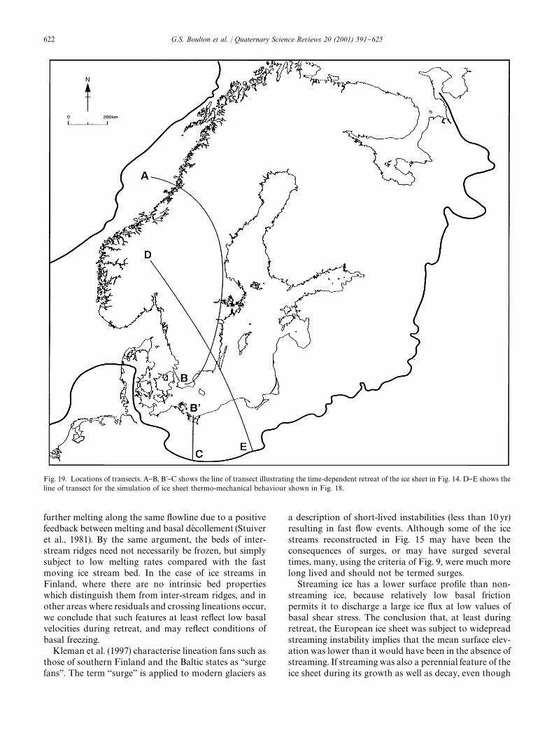
Fig. 19. Locations of transects. A}B, B@}C shows the line of transect illustrating the time-dependent retreat of the ice sheet in Fig. 14. D}E shows theline of transect for the simulation of ice sheet thermo-mechanical behaviour shown in Fig. 18.

further melting along the same #owline due to a positivefeedback between melting and basal deH collement (Stuiveret al., 1981). By the same argument, the beds of inter-stream ridges need not necessarily be frozen, but simplysubject to low melting rates compared with the fastmoving ice stream bed. In the case of ice streams inFinland, where there are no intrinsic bed propertieswhich distinguish them from inter-stream ridges, and inother areas where residuals and crossing lineations occur,we conclude that such features at least re#ect low basalvelocities during retreat, and may re#ect conditions ofbasal freezing.

Kleman et al. (1997) characterise lineation fans such asthose of southern Finland and the Baltic states as `surgefansa. The term `surgea is applied to modern glaciers as

a description of short-lived instabilities (less than 10 yr)resulting in fast #ow events. Although some of the icestreams reconstructed in Fig. 15 may have been theconsequences of surges, or may have surged severaltimes, many, using the criteria of Fig. 9, were much morelong lived and should not be termed surges.

Streaming ice has a lower surface pro"le than non-streaming ice, because relatively low basal frictionpermits it to discharge a large ice #ux at low values ofbasal shear stress. The conclusion that, at least duringretreat, the European ice sheet was subject to widepreadstreaming instability implies that the mean surface elev-ation was lower than it would have been in the absence ofstreaming. If streaming was also a perennial feature of theice sheet during its growth as well as decay, even though


individul streams may have been short lived, the meanelevation of the ice sheet would have been signi"cantlyless than inferred from ice sheet models which do notinclude streaming. This may explain the con#ict betweenreconstructions of European ice sheet surface elevationsderived from glaciological models of the ice sheet, such asthose of Denton and Hughes (1981) and Boulton andPayne (1994 ), which suggest summit elevations at theglacial maximum of 3400 and 3200m, respectively, andreconstructions by Lambeck et al. (1998) based on mod-els of Earth rheology which invert relative sea level datato infer ice sheet loads and which suggest summit elev-ations of about 1600m.

This con#ict may require us to revise our view of thelong-term behaviour of ice sheets. Low summit elev-ations may have been a consequence of low slope icesheets #owing over a deforming bed (Boulton et al.(1985), suggest that such a process could depress summitelevations to about 2100m in Europe) but is also possiblethat low elevations are maintained as a consequence ofperennial streaming. Most models which have been usedhitherto to simulate the time-dependent behaviour of icesheets have not included streaming. As a consequence,simulated ice sheets change only slowly and are never farfrom a steady state. It seems likely that, in reality, theydisplayed highly dynamic, streaming behaviour whichvaried strongly on short timescales and that they werevery far from a steady state. They should therefore bemodelled in a way which captures the instabilities whichgenerate streaming behaviour.

Note added in proof

New evidence from northern Finland (Helmens et al.,2000) appears to con"rm the pattern of ice-sheet #uctu-ation shown in Fig. 18 and the views of Group A.

Acknowledgements

We are grateful for helpful discussions to BarbaraWohlfarth, Svante BjoK rk, Nick Hulton, Anto Raukas,Jonathon Perry, Lars ForsstroK m, Michael Houmark-Nielsen and JuK rgen Ehlers.

References

Aario, R., ForsstroK m, L., 1979. Glacial stratigraphy of Koillismaa andNorth Kainuu, Finland. Fennia 157 (2), 1}49.

Alley, R.B., Blankenship, D.D., Rooney, S.T., Bentley, C.R. 1987. Con-tinuous till deformation beneath ice sheets. The Physical Basis of IceSheet Modelling. Proceedings of the Vancouver Symposium, Au-gust 1987. IAHS Publications, Vol. 170, pp. 81}91.

Andersen, B.G., 1987. Quaternary research in Norway 1960}1986.Boreas 16, 327}338.

Andren, T., BjoK rck, J., Johnsen, S., 1999. Correlation of Swedish glacialvarves with the Greenland (GRIP) oxygen isotope record. Journalof Quaternary Science 14, 361}371.

Bard, E., Arnold, M., Fairbanks, R.G., Hamelin, B., 1993. 230Th/234Uand 14C ages obtained by mass spectrometry on corals. Radiocar-bon 35, 191}199.

Berglund, B.E., Hakansson, S., Lagerlund, E., 1976. Radiocarbon-datedmammoth "nds in South Sweden. Boreas 5, 177}191.

BjoK rck, S., Wohlfarth, B., Possnert, 1995. 14C AMS measurements fromthe Late Weichselian part of the Swedish Time Scale. QuaternaryInternational 27, 11}18.

Bond, G., Broecker, W., Johnsen, S., McManus, J., Labeyrie, L., Jouzel,J., Bonani, G., 1993. Correlations between climate records fromNorth Atlantic sediments and Greenland ice. Nature 365, 143}147.

Boulton, G.S., 1972. The role of thermal regime in glacial sedimenta-tion. In: Price, R.J., Sugden, D.E. (Eds.), Polar Geomorphology.Institute of British Geographers, Special Publication Vol. 4, pp.1}19.

Boulton, G.S., 1987. A theory of drumlin formation by subglacialdeformation. In: Rose, J., Menzies, J. (Eds.), Drumlins. Balkema,Rotterdam, pp. 25}80.

Boulton, G.S., 1996. Theory of glacial erosion, transport and depositionas a consequence of subglacial sediment deformation. Journal ofGlaciology 42 (140), 43}62.

Boulton, G.S., Clark, C.D., 1990a. A highly mobile Laurentide ice sheetrevealed by satellite images of glacial lineations. Nature 346,813}817.

Boulton, G.S., Clark, C.D., 1990b. The Laurentide ice sheet through thelast glacial cycle: the topology of drift lineations as a key to thedynamic behaviour of former ice sheets. Transactions of the RoyalSociety of Edinburgh: Earth Sciences 81, 327}347.

Boulton, G.S., Jones, A.S., 1979. Stability of temperate ice caps and icesheets resting on beds of deformable sediment. Journal of Glaciol-ogy 24, 29}43.

Boulton, G.S., Payne, A., 1994. Mid-latitude ice sheets through the lastglacial cycle: glaciological and geological reconstructions. In: Du-plessy, J.-C., Spyridakis, M.-T. (Eds.), Long-term Climatic Vari-ations. NATO ASI Series I, Vol. 22, pp. 177}212.

Boulton, G.S., Caban, P.E., van Gijssel, K., 1995. Groundwater #owbeneath ice sheets: Part I - Large-scale patterns. Quaternary ScienceReview 4, 545}562.

Boulton, G.S., Hulton, N., Vautravers, M., 1995. Ice sheet models astools for palaeoclimatic analysis: the European ice sheet through thelast glacial cycle. Annals of Glaciology 21, 103}110.

Boulton, G.S., Smith, G.D., Jones, A.S., Newsome, J., 1985. Glacialgeology and glaciology of the last mid-latitude ice sheets. Journal ofthe Geological Society, London 142, 447}474.

Chamberlin, T.C., 1895. Glacial phenomena of North America. In:Geikie, J. (Ed.), The Great Ice Age, 2nd Edition. Appleton, NewYork, pp. 724}775.

Charlesworth, J.K., 1957. The Quaternary Era. Arnold, London.Chebotareva, N.S. (Ed.), 1977. The Structure and Dynamics of the Last

Ice Sheet of Europe. Nauka, Moscow, 143 pp (in Russian).De Geer, G., 1940. Geochronologie Suecica Principles. Kungliga

Svenska Vetenskaps-Akademiens Handlingar 3 18 (6), 367 pp.Dongelmans, P., 1997. Glacier dynamics of the Fennoscandian ice

sheet: a remote sensing study. Unpublished Ph.D. Thesis, Universityof Edinburgh.

Ehlers, J., 1990. Reconstrcucting the dynamics of the north west Euro-pean Pleistocene ice sheets. Quatrernary Science Reviews 9, 71}83.

Fairbanks, R.G., 1989. A 17,000 year glacio-eustatic sea level record:in#uence of glacial melting rate on the Younger Dryas event anddeep ocean circulation. Nature 342, 637}642.

ForsstroK m, L., Eronen, M., 1991. New information about the Eemianand Early Weichselian in Finland. Striae 34, 31}38.

Freden, C. (Ed.), 1994. National Atlas of Sweden. Geology. SNA,Stockholm.


GluK ckert, G., 1974. The Kuusamo drumlin "eld, northern Finland.Bulletin of the Geological Society of Finland 46, 37}42.

Hang, T., 1997. Clay varve chronology in the Eastern Baltic area.Geologiska FoK reningens I Stockholm ForhaK ndlingar 119, 295}300.

Hatterstrand, C., Kleman, J., 1999. Ribbed moraine formation. Quater-nary Science Reviews 18, 43}61.

Helmens, K.F., RaK saK nen, M.E., Johansson, P.W., Junger, H., Korjonen,K., 2000. The Last Interglacial}Glacial cycle in NE Fennoscandia:a nearly continuous record from Sokli (Finnish Lapland). Quater-nary Science Reviews 19, 1605}1623.

Hillefors, A., 1974. The stratigraphy and genesis of the Dosebacka andEllesbo drumlins. Geologiska Foreningens i Stockholm Forhan-dlngar 96, 355}374.

Hirvas, H., Nenonen, K., 1985. The till stratigraphy of Finland. IN-QUA Till Symposium, Finland 1985. Geological Dsurvey of Fin-land, Special Paper 3, 49}63.

Holtedahl, H., 1993. Marine geology of the Norwegian continentalmargin. Geological Survey of Norway, Trondheim, Norway, 150 pp.

Houmark-Nielsen, M., 1987. Pleistocene stratigraphy and glacial his-tory of the central part of Denmark. Bulletin of the GeologicalSociety of Denmark 36 (1}2), 189.

Hughes, T.J., 1981. Numerical reconstructions of paleo-ice sheets. In:Denton, G.H., Hughes, T.J. (Eds.), The Last Great Ice Sheets. Wiley,New York, pp. 222}274.

Hughes, T.J., 1982. On the disintegration of ice shelves: The role ofthinning. Annals of Glaciology 3, 146}151.

Imbrie, J., Hays, J.D., Martinson, D.G., McIntyre, A., Mix, A.C., Mor-ley, J.J., Pisias, N.G., Prell, W.L., Shackleton, N.J., 1984. The orbitaltheory of Pleistocene climate: support from a revised chronology ofthe marine 180 record. In: Berger, A., Imbrie, J., Hays, J., Kukla, G.,Saltzman, B. (Eds.), Milankovitch and Climate. D. Reidel, Dor-drecht, pp. 269}306.

Johnsen, S.J., Clausen, H.B., Dansgaard, W., Fuhrer, K., Gundestrup,N., Hammer, C.U., Iversen, P., Jouzel, J., Stau!er, B., Ste!ensen,J.P., 1992. Irregular glacial interstadials recorded in a new Green-land ice core. Nature 359, 311}313.

Kamb, B., Engelhardt, H.F., 1989. Flow mechanics of West Antarcticice streams: observations by borehole geophysics. EOS 70,1081.

King, E.L., Rokoengen, K., Gunleiksrud, T., 1987. Quaternary seismos-tratigraphy of the mid Norwegian Shelf, 65@N-67@, 30@N. A TillTongue Stratigraphy. IKU, Publ. 114, 58 pp.

King, E.L., Sejrup, H.P., Ha#idason, H., Elvehoi, A., Aarseth, I., 1996.Quaternary seismic stratigraphy of the North Sea Fan; glacially fedgravity #ow aprons, hemipelagic sediments and large submarineslides. Marine Geology 130, 293}315.

Kleman, J., 1990. On the use of glacial striae for reconstruction ofpalaeo-ice sheet #ow patterns. Geogra"ska Annaler 72A,217}236.

Kleman, J., 1992. The palimpsest glacial landscape in northwesternSweden * Late Weichselian deglaciation landforms and traces ofof older west-centred ice sheets. Geogra"ska Annaler 74A,305}325.

Kleman, J., BorgstroK m, L., 1990. The boulder "elds of mount Pulufjal-let, west-central Sweden. Geogra"ska Annaler 72A (1), 63}78.

Kleman, J., HaK tterstrand, C., BorgstroK m, I., Stroeven, A., 1997. Fennos-candian palaeoglaciology reconstructed using a glacial geologicalinversion model. Journal of Glaciology 43, 283}299.

Korpela, K., 1969. Die Weichsel-Eiszieit und ihr Interstadial inPerapohjola im Licht von submoranen Sedimenten. Annals of theAcademy of Sciences Fennicae A III 99, 108.

Kozarski, S., 1986. Timescales and the rhythm of Vistulian geomorphicevents in the Polish lowlands. Czasopismo Geogra"czne 57,247}270.

Kozarski, S., 1988. Time and dynamics of the last Scandinavian icesheet retreat from northwestern Poland. Geographica Polonica 55,91}101.

Krasnov, I.I., 1971. The map of Quaternary deposits of Europe andterritories surrounding it, scale 1 : 1,500,000. Ministry of GeologySSSR.

Kromer, B., Becker, B., 1993. German oak and pine 14C calibration,7200-9439 BC. Radiocarbon 35, 125}135.

Kroon, D., Austin, W.E.N., Chapman, M.R., Ganssen, G.M., 1997.Deglacial surface circulation changes in the northeast Atlantic:temperature and salinity records o! NW Scotland on a centuryscale. Palaeoceanography 12, 755}763.

Kvasov, D.D., 1978. The Barents ice sheet as a relay regulatorof glacial-interglacial alternation. Quaternary Research 9,288}299.

LagerbaK ck, R., 1988. The Veiki moraines in northern Sweden-wide-spread evidence of an early Weichselian deglaciation. Boreas 17,469}486.

Lagerlund, E., 1980 Litostratigra"sk indelning av VaK stska> nes Pleis-tocen och en ny glaciationsmodell foK r Weichsel. University of Lund,Department of Quaternary Geology, Thesis 5, 106 pp.

Lagerlund, E., Houmark-Nielsen, M., 1993. Timing and pattern of thelast deglaciation in the Kattegat region, southwest Scandinavia.Boreas 22, 337}347.

Lambeck, K., Smither, C., Johnston, P., 1998. Sea-level change, glacialrebound and mantle viscosity for northern Europe. GeophysicalJournal International 134, 102}144.

Landvik, J.Y., Bondevik, S., Elvehoi, A., Fjeldskaar, W., Mangerud,J., Salvigsen, O., Siegert, M., Svendsen, J.-I., Vorren, T.,1998. The last glacial maximum of Svalbard and the Barents Seaarea: ice sheet extent and con"guration. Quaternary Science Re-views 17, 43}75.

Larsen, E., Lysa, A., Demidov, I., Funder, S., Houmark-Nielsen, M.,Kjaer, K.H., Murray, A.S., 1999. Age and extent of the Scandinavianice sheet in northwest Russia. Boreas 28, 115}132.

Liedtke, H., 1981. Die nordischen Vereisungen in Mitteleuropa. For-schungen z. dt. Landeskunde, 204, (2nd edition).

Lundqvist, J., 1974. Outlines of the Weichsel Glacial in Sweden. Geol.FoK ren. Stockholm FoK rhandl. 96, 327}339.

Lundqvist, J., 1986. Stratigraphy of the central area of the Scandinavianglaciation. Quaternary Sciences Reviews 5, 251}268.

Lundqvist, J., 1992. Glacial stratigraphy in Sweden. In: Kauranne,K. (Ed.), Glacial Stratigraphy, Engineering Geology and EarthConstruction. Geological Survey of Finland, Special Paper 15,43}59.

Mangerud, J., 1991. The Scandinavian ice sheet through the last inter-glacial/glacial cycle. In: Frenzel, B. (Ed.), Klimageschichtliche Prob-leme der letzten 130,000 Jahre. G. Fischer. Stuttgart, New York, pp.307}330.

Mangerud, J., Larsen, E., Longva, O., Sonstegaard, E., 1979.Glacial history of western Norway 15,000}10,000 BP. Boreas 8,179}187.

Mojski, J.E., 1992. Vistulian stratigraphy and TL dates in Poland.Sveriges Geologiska UndersoK kning, Series Ca 81, 195}200.

Nordkalott Project, 1986. Map of Quaternary geology, sheet 5: Ice #owdirections, Northern Fennoscandia. Geological Surveys of Finland,Norway and Sweden. Uppsala.

Paterson, W.S.B., 1994. The Physics of Glaciers, 3rd edition. Pergamon,Oxford.

Perry. J.E.H., 1998. Reconstructing the character of the eastern sector ofthe Scandinavian ice sheet using remote sensing. UnpublishedPh.D. Thesis. University of Edinburgh.

Punkari, M., 198. Glacial geomorphology and dynamics in the easternparts of the Baltic Shield interpreted using Landsat imagery. Photo-grammetric Journal of Finland 9, 77}93.

Punkari, M., 1984. The relations between glacial dynamics and tills inthe eastern part of the Baltic Shield. Striae 20, 49}54.

Punkari, M., 1985. Glacial geomorphology and dynamics in SovietKarelia interpreted by means of satellite imagery. Fennia 163,113}153.


Punkari, M., 1993. Modelling of the dynamics of the Scandinavian icesheet using remote sensing and GIS methods. In: Aber, J. (Ed.),Glaciotectonics and Mapping Glacial Deposits. Proceedings of theINQUA Comission on Formation and Properties of Glacial De-posits. Canadian Plains Research Center, University of Regina, pp.232}250.

Punkari, M., 1995. Function of the ice streams in the Scandinavian icesheet: analyses of glacial geological data from southwestern Fin-land. Transactions of the Royal Society of Edinburgh: EarthSciences 85, 283}302.

Punkari, M., ForsstroK m, L., 1995. Organic remains in Finnish sub-glacial Sediments. Quaternary Research 43, 414}425.

Ralska-Jasiewiczowa, M., Rzetkowska, A., 1987. Pollen macrofossilstratigraphy of fossil lake sediments at Niechorze I. ActaPalaeobotanica 22, 153}158.

Reeh, N., 1982. A plasticity theory approach to the steady-state shape ofa three-dimensional ice sheet. Journal of Glaciology 28, 431}455.

Ringberg, B., 1988. Late Weichselian geology in southernmost Sweden.Boreas 17, 243}263.

Rise, L., Roekoengen, K., Svttem, J., Bugge, T., 1988. Thickness ofQuaternary deposits on the mid-Norwegian Continental Shelf. Mapin scale 1 : 1.000.000. IKU Publ. 119.

Robin, G., de, Q., 1979. Formation, #ow and disintegration of iceshelves. Journal of Glaciology 24, 259}271.

Roekoengen, K., Bugge, T., Lofaldi, M., Vigran, J.O., 1979. Quaternarygeology and deglaciation of the continental shelf o! Troms, NorthNorway. Boreas 8, 217}227.

Roekoengen, K., Rise, L., Bugge, T., Svttem, J., 1988. Bedrock geologyof the mid Norwegian continental shelf. Map in scale 1 : 1.000.000.IKU Publ. 118.

Rose, J., Letzer, J.M., 1977. Superimposed drumlins. Journal of Glaciol-ogy 18 (80), 471}480.

Sandgren, P., Hang, T., Snowball, I.F., 1997. A late Weichseliangeomagnetic record from Lake Tamula, SE Estonia. GeologiskaFoK reningens I Stockholm ForhaK ndlingar 119, 279}284.

Sauramo, M., 1918. Geochronologische Studien uber die spaK tglazialeZeit in Sud"nnland. Fennia 41, 1}44.

Sauramo, M., 1923. Studies on the Quaternary varve sediments insouthern Finland. Fennia 44 (1), 1}164.

Sejrup, H.P., Aarseth, I., Ellingsen, K.L., Reither, E., Jansen, E., Lovlie,R., Bent, A., Brigham-Grette, J., Larsen, E., Stoker, M., 1987. Quat-ernary stratigraphy of the Fladen area, central North Sea: a multi-disciplinary study. Journal of Quaternary Science 2, 35}58.

Sejrup, H.P., Ha#idason, H., Aarseth, I., King, E., Forsberg, C.F., Long,D., Roekoengen, K., 1994. Late Weichselian glaciation history of thenorthern North Sea. Boreas 23, 1}13.

Sejrup, H.P., King, E.L., Aarseth, I., Ha#idason, H., Elvehoi, A., 1996.Quaternary erosional and depositional processes: western Norwe-gian fjords, Norwegian Channel and North Sea Fan. GeologicalSociety of London 117, 187}202.

Sejrup, H.P., Landvik, J.Y., Larsen, E., Janocko, J., Eiriksson, J., King,E.L., 1998. The Jaeren rea, a border zone of the Norwegian Channelice stream. Quaternary Science Reviews 17, 801}812.

Sejrup, H.P., Larsen, E., Landvik, J., King, E.L., Ha#idson, H., Nesje,A., 2000. Quaternary glaciations in southern Fennoscandia: evid-ence form southwestern Norway and the northern North Sea re-gion. Quaternary Science Reviews 19, 667}685.

Shabtaie, S., Bentley, C.R., 1987. West Antarctic ice streams draininginto the Ross Ice Shelf: con"guration and mass balance. Journal ofGeophysical Research 92 (B2), 1311}1336.

Shabtaie, S., Whillans, I.M., Bentley, C.R., 1987. The morphology og IceStreams A, B and C, West Antarctica, and their environs. Journal ofGeophysical Research 92 (B9), 8865}8883.

Sj+rring, S., 1983. The glacial history of Denmark. In: Ehlers, J. (Ed.),Glacial Deposits in North-West Europe. Balkema, Rotterdam, pp.163}179.

Stephenson, S.N., Bindschadler, R.A., 1990. Is ice-stream evolutionrevealed by satellite imagery? Annals of Glaciology 14,273}277.

StroK mberg, B., 1985. Revision of the lateglacial Swedish varve chrono-logy. Boreas 14, 101}105.

StroK mberg, B., 1990. A connection between the clay varve chronologiesin Sweden and Finland. Annales Academiae Scientiarum Fennicae154A (III), 32.

StroK mberg, B., 1994. Younger Dryas deglaciation at Mt. Billingen, andclay varve dating of the Younger Dryas/Preboreal transition.Boreas 23, 177}193.

Stuiver, M., Denton, G.H., Hughes, T.J., Fastook, J.L., 1981. History ofthe marine ice sheet in West Antarctica during the last glaciation:a working hypothesis. In: Denton, G.H., Hughes, T.J. (Eds.), TheLast Great Ice Sheets. Wiley, New York, pp. 319}436.

Stuiver, M., Reimer, P.J., 1993. Extended 14C data base andrevised CALIB 3.0 14C age calibration program. Radiocarbon 35,215}230.

Sutinen, R., 1992. Glacial deposits, their electrical properties and sur-veying by image interpretation and ground penetrating radar. Geo-logical Survey of Finland, Bulletin 359, 123.

Svendsen, J.I., Mangerud, J., 1992. Paleoclimatic inferences from glacial#uctuations on Svalbard during the last 20,000 years. ClimateDynamics 6, 213}220.

Tanner, V., 1915. Studier oK fver kvartaK rsystemet i Fennoskandias nor-dliga delar. Fennia 36, 815.

Torell, O., 1865. Foreword. In: HolmstroK m, L.P. (Ed.), IakttagelseroK fver maK rken: Ska> ne efter istiden. Chronholmska Boktryckeriet,MalmoK .

Ukkonen, P., Lunkka, J.P., Jungner, H., Donner, J., 1999. Newradiocarbon dates from Finnish mammoths indicating large ice-freeareas in Fennoscandia during the middle Weichselian. Journal ofQuaternary Science 14, 711}714.

Valen, V., Mangerud, J., Larsen, E., Hufthammer, A.K., 1996.Sedimentology and stratigraphy in the cave Hamnsundhelleren,western Norway. Journal of Quaternary Science 11,185}201.

Van der Veen, J., 1986. Numerical modelling of ice shelves and icetongues. Annales Geophysicae 4B (1), 45}54.

Vorren, T.O., Vorren, K.-D., Alm, T., Gulliksen, S., L+vlie, R., 1988. Thelast deglaciation (20,000 to 11,000 B.P.) on And+ya, northern Nor-way. Boreas 17, 41}77.

Whillans, I.M., Bolzan, J., Shabtaie, S., 1987. Velocity of ice streamB and C, Antarctica. Journal of Geophysical Research 92 (B9),8895}8902.

Wohlfarth, B., Bj+rck, S., Possner, G., 1995. The Swedish time scale-apotential calibration tool for the radiocarbon timescale during theLate Weichselian. Radiocarbon 37, 347}359.


Palaeoglaciology of an ice sheet through a glacial cycle ... 2006 readings/Scandinavia and... ·...

Documents

Transcript of Palaeoglaciology of an ice sheet through a glacial cycle ... 2006 readings/Scandinavia and... ·...