Paired Analysis of Time-Series Studies Using Concentration ... · Paired Analysis of Time-Series...

MetaboAnalyst Tutorial 4

Paired Analysis of Time-Series Studies Using Concentration Data

By Nick Psychogios ([email protected])

Last update: 4/15/2009

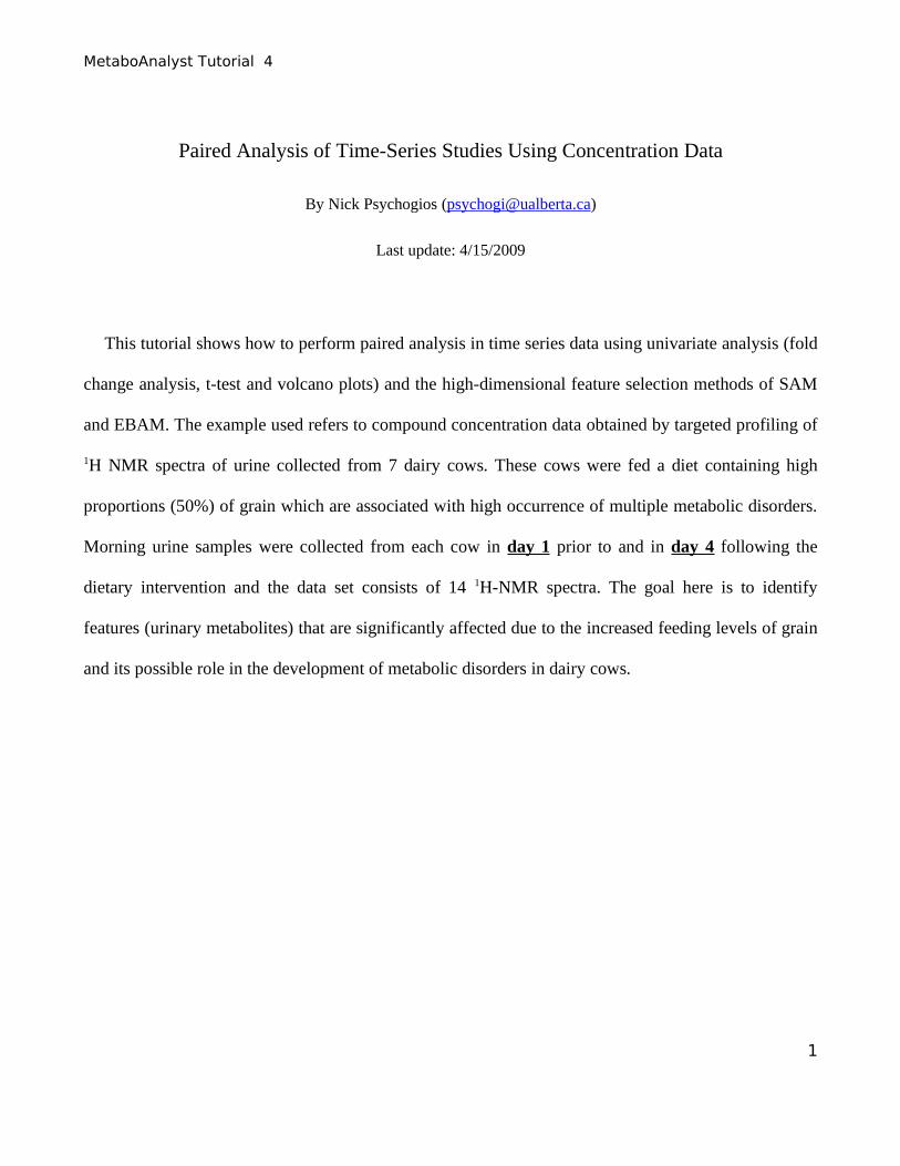
This tutorial shows how to perform paired analysis in time series data using univariate analysis (fold

change analysis, t-test and volcano plots) and the high-dimensional feature selection methods of SAM

and EBAM. The example used refers to compound concentration data obtained by targeted profiling of

1H NMR spectra of urine collected from 7 dairy cows. These cows were fed a diet containing high

proportions (50%) of grain which are associated with high occurrence of multiple metabolic disorders.

Morning urine samples were collected from each cow in day 1 prior to and in day 4 following the

dietary intervention and the data set consists of 14 1H-NMR spectra. The goal here is to identify

features (urinary metabolites) that are significantly affected due to the increased feeding levels of grain

and its possible role in the development of metabolic disorders in dairy cows.

1

mailto:[email protected]


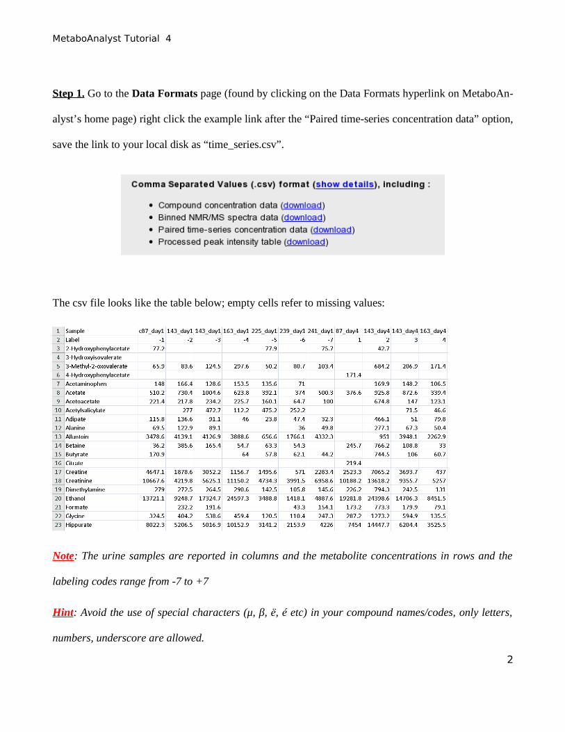
Step 1. Go to the Data Formats page (found by clicking on the Data Formats hyperlink on MetaboAn-

alyst’s home page) right click the example link after the “Paired time-series concentration data” option,

save the link to your local disk as “time_series.csv”.

The csv file looks like the table below; empty cells refer to missing values:

Note: The urine samples are reported in columns and the metabolite concentrations in rows and the

labeling codes range from -7 to +7

Hint: Avoid the use of special characters (μ, β, ë, é etc) in your compound names/codes, only letters,

numbers, underscore are allowed.

2


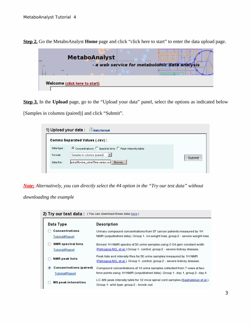
Step 2. Go the MetaboAnalyst Home page and click “click here to start” to enter the data upload page.

Step 3. In the Upload page, go to the “Upload your data” panel, select the options as indicated below

[Samples in columns (paired)] and click “Submit”.

Note: Alternatively, you can directly select the #4 option in the “Try our test data” without

downloading the example

3


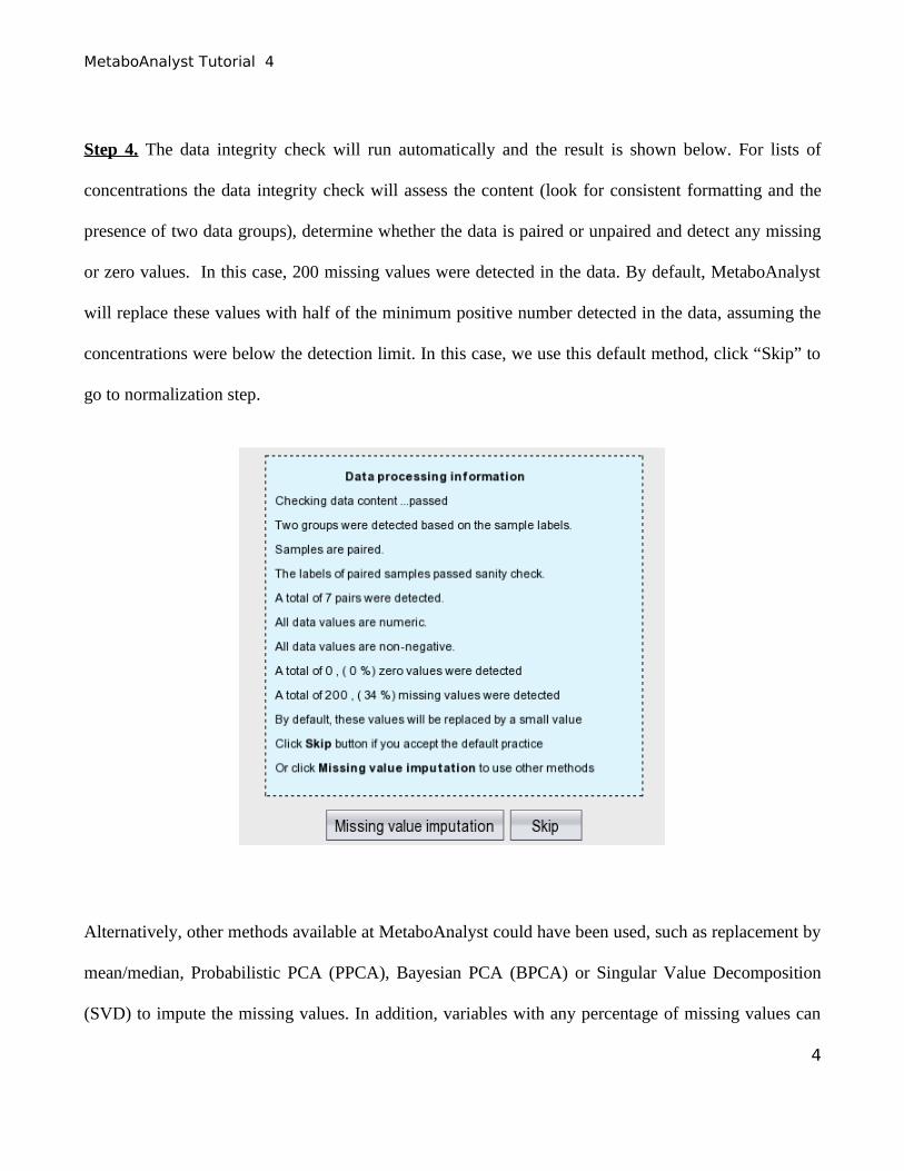
Step 4. The data integrity check will run automatically and the result is shown below. For lists of

concentrations the data integrity check will assess the content (look for consistent formatting and the

presence of two data groups), determine whether the data is paired or unpaired and detect any missing

or zero values. In this case, 200 missing values were detected in the data. By default, MetaboAnalyst

will replace these values with half of the minimum positive number detected in the data, assuming the

concentrations were below the detection limit. In this case, we use this default method, click “Skip” to

go to normalization step.

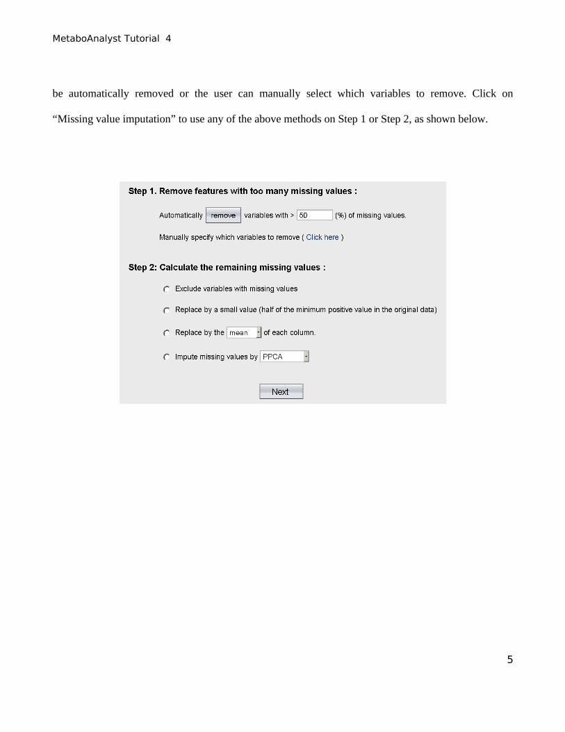
Alternatively, other methods available at MetaboAnalyst could have been used, such as replacement by

mean/median, Probabilistic PCA (PPCA), Bayesian PCA (BPCA) or Singular Value Decomposition

(SVD) to impute the missing values. In addition, variables with any percentage of missing values can

4


be automatically removed or the user can manually select which variables to remove. Click on

“Missing value imputation” to use any of the above methods on Step 1 or Step 2, as shown below.

5


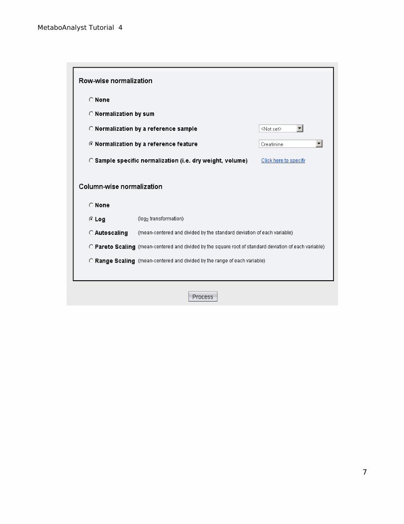
Step 5. Now we arrive at the data normalization step. The internal data structure is transformed now to

a table with each column representing a urine sample (from a dairy cow) and each row representing a

feature (a compound with a concentration). With the data structured in this format, two types of data

normalization protocols - row-wise normalization and column-wise normalization -- may be used.

These are often applied sequentially to reduce systematic variance and to improve the performance for

downstream statistic analysis. Row-wise normalization aims to normalize each sample (row) so that it

is comparable to the other. In the present example, even though the samples are tabled in columns we

still refer to this normalization procedure as row-wise normalization. For row-wise normalization

MetaboAnalyst supports normalization to a constant sum, normalization to a reference sample

(probabilistic quotient normalization), normalization to a reference feature (creatinine or an internal

standard) or sample-specific normalization (dry weight or tissue volume). In contrast to row-wise

normalization, column-wise normalization aims to make each feature (column) more comparable in

magnitude to each other. Four widely-used methods are offered in MetaboAnalyst - log transformation,

auto-scaling, Pareto scaling, and range scaling.

Urine concentrations are usually normalized by creatinine concentration to adjust for the dilution effect

(select option 4 - Normalization by a reference feature and choose “creatinine” from the drop-down

menu). After deciding to normalize by reference feature for our row-wise (sample) normalization we

then choose “Log normalization” for our column normalization to make the metabolite concentration

values more comparable among different compounds.

6


7


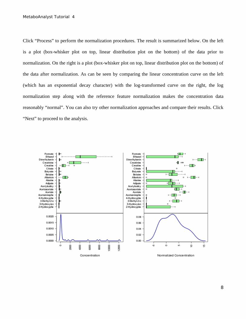
Click “Process” to perform the normalization procedures. The result is summarized below. On the left

is a plot (box-whisker plot on top, linear distribution plot on the bottom) of the data prior to

normalization. On the right is a plot (box-whisker plot on top, linear distribution plot on the bottom) of

the data after normalization. As can be seen by comparing the linear concentration curve on the left

(which has an exponential decay character) with the log-transformed curve on the right, the log

normalization step along with the reference feature normalization makes the concentration data

reasonably “normal”. You can also try other normalization approaches and compare their results. Click

“Next” to proceed to the analysis.

8


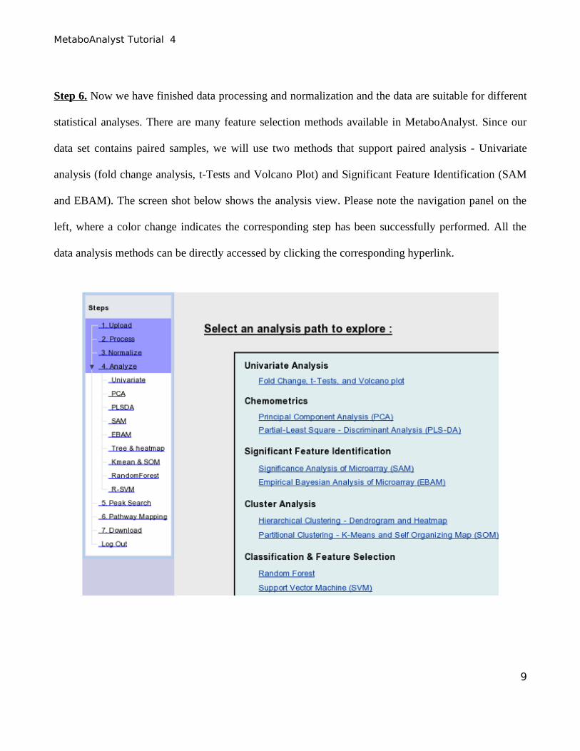
Step 6. Now we have finished data processing and normalization and the data are suitable for different

statistical analyses. There are many feature selection methods available in MetaboAnalyst. Since our

data set contains paired samples, we will use two methods that support paired analysis - Univariate

analysis (fold change analysis, t-Tests and Volcano Plot) and Significant Feature Identification (SAM

and EBAM). The screen shot below shows the analysis view. Please note the navigation panel on the

left, where a color change indicates the corresponding step has been successfully performed. All the

data analysis methods can be directly accessed by clicking the corresponding hyperlink.

9


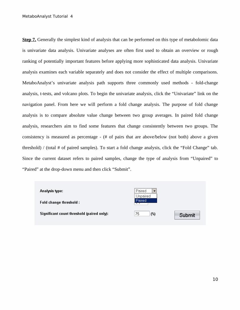
Step 7. Generally the simplest kind of analysis that can be performed on this type of metabolomic data

is univariate data analysis. Univariate analyses are often first used to obtain an overview or rough

ranking of potentially important features before applying more sophisticated data analysis. Univariate

analysis examines each variable separately and does not consider the effect of multiple comparisons.

MetaboAnalyst’s univariate analysis path supports three commonly used methods - fold-change

analysis, t-tests, and volcano plots. To begin the univariate analysis, click the “Univariate” link on the

navigation panel. From here we will perform a fold change analysis. The purpose of fold change

analysis is to compare absolute value change between two group averages. In paired fold change

analysis, researchers aim to find some features that change consistently between two groups. The

consistency is measured as percentage - (# of pairs that are above/below (not both) above a given

threshold) / (total # of paired samples). To start a fold change analysis, click the “Fold Change” tab.

Since the current dataset refers to paired samples, change the type of analysis from “Unpaired” to

“Paired” at the drop-down menu and then click “Submit”.

10


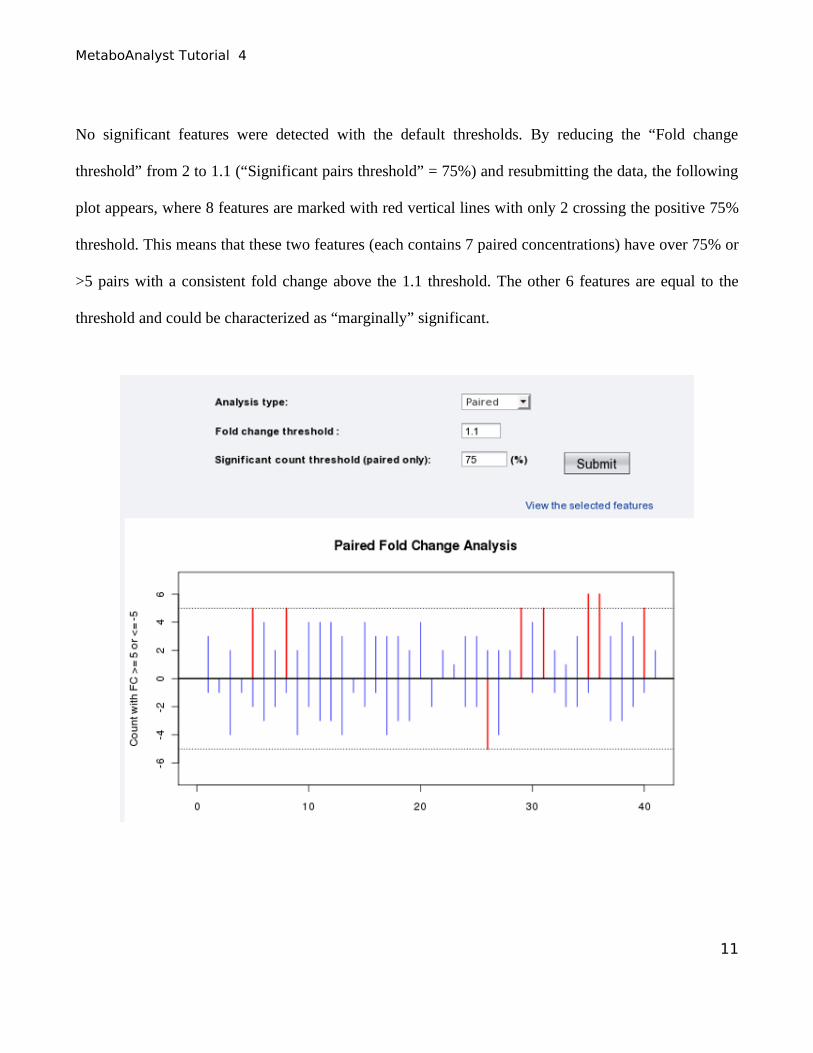
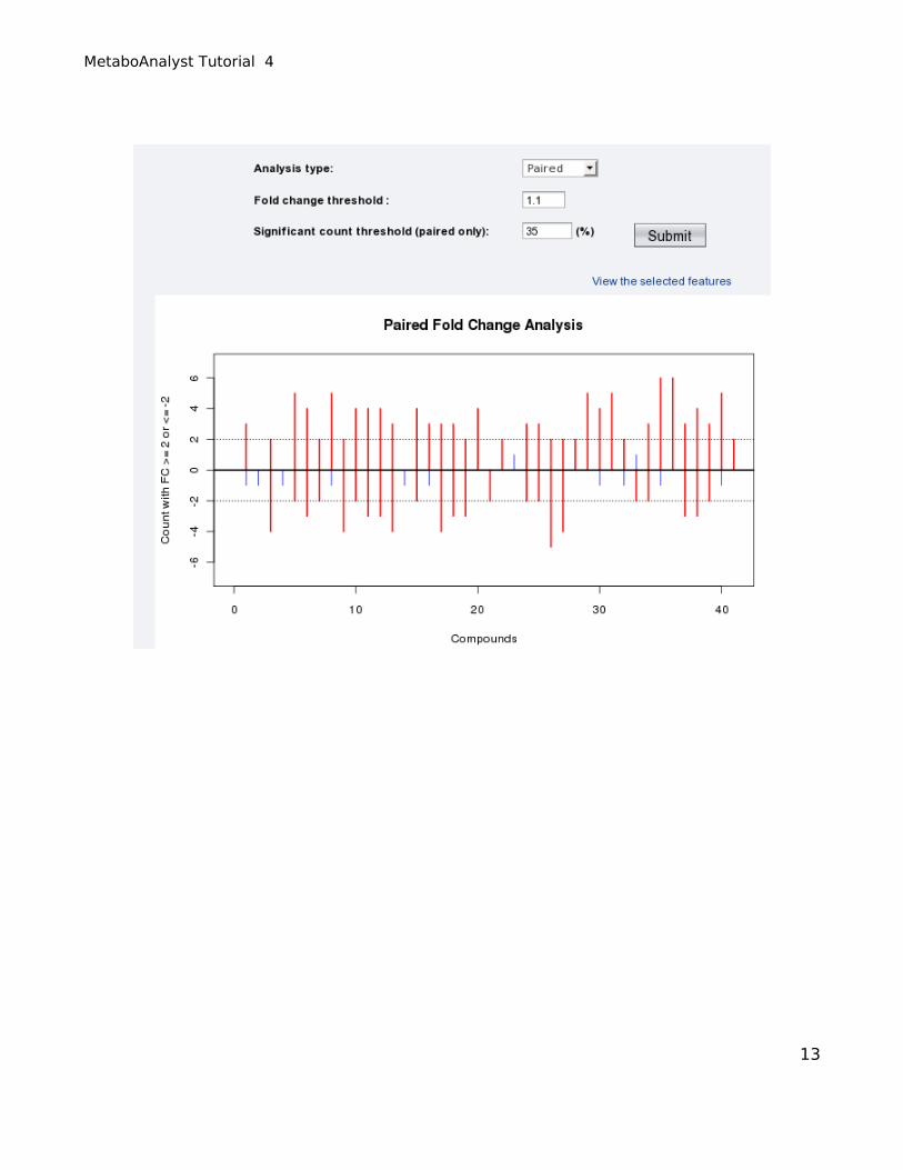
No significant features were detected with the default thresholds. By reducing the “Fold change

threshold” from 2 to 1.1 (“Significant pairs threshold” = 75%) and resubmitting the data, the following

plot appears, where 8 features are marked with red vertical lines with only 2 crossing the positive 75%

threshold. This means that these two features (each contains 7 paired concentrations) have over 75% or

>5 pairs with a consistent fold change above the 1.1 threshold. The other 6 features are equal to the

threshold and could be characterized as “marginally” significant.

11


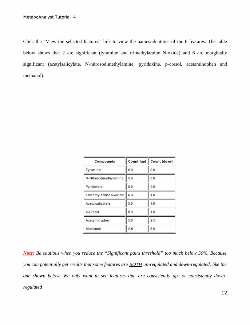
Click the “View the selected features” link to view the names/identities of the 8 features. The table

below shows that 2 are significant (tyramine and trimethylamine N-oxide) and 6 are marginally

significant (acetylsalicylate, N-nitrosodimethylamine, pyridoxine, p-cresol, acetaminophen and

methanol).

Note: Be cautious when you reduce the “Significant pairs threshold” too much below 50%. Because

you can potentially get results that some features are BOTH up-regulated and down-regulated, like the

one shown below. We only want to see features that are consistently up- or consistently down-

regulated12


13


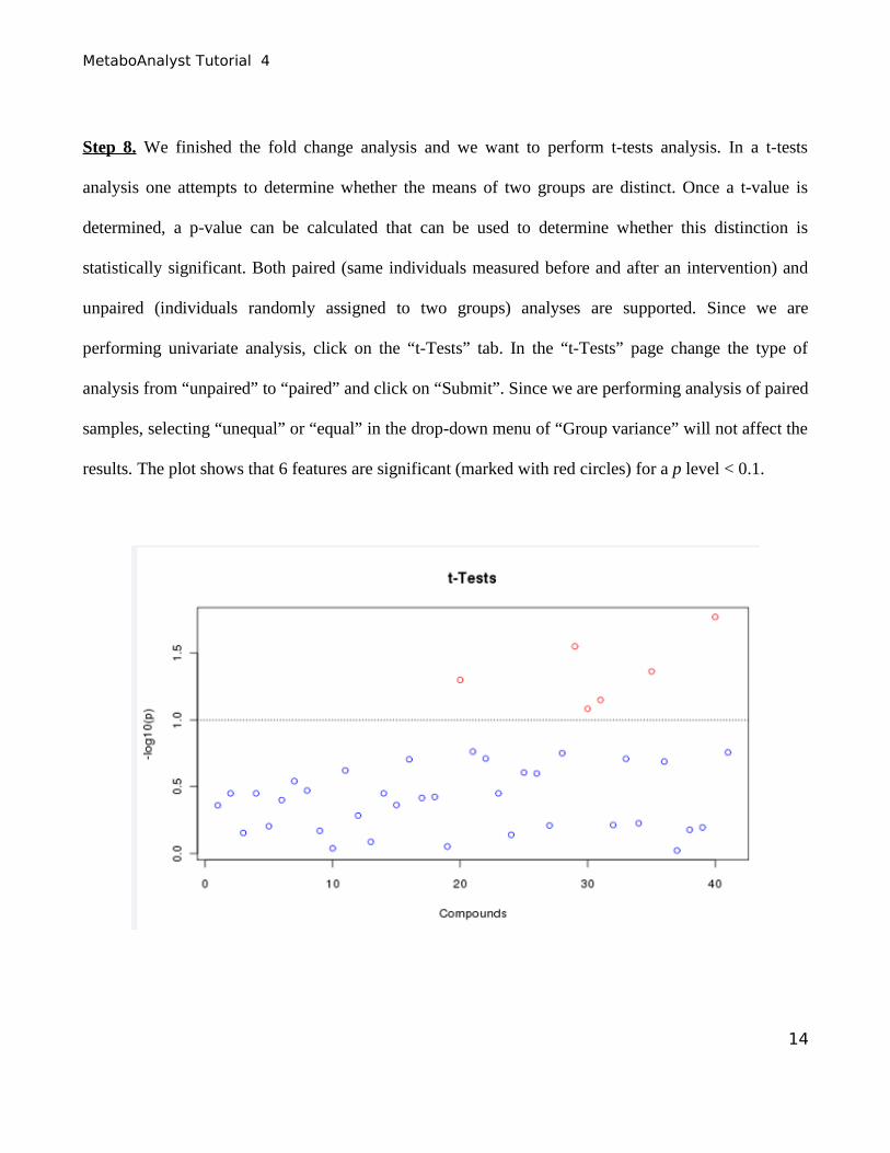
Step 8. We finished the fold change analysis and we want to perform t-tests analysis. In a t-tests

analysis one attempts to determine whether the means of two groups are distinct. Once a t-value is

determined, a p-value can be calculated that can be used to determine whether this distinction is

statistically significant. Both paired (same individuals measured before and after an intervention) and

unpaired (individuals randomly assigned to two groups) analyses are supported. Since we are

performing univariate analysis, click on the “t-Tests” tab. In the “t-Tests” page change the type of

analysis from “unpaired” to “paired” and click on “Submit”. Since we are performing analysis of paired

samples, selecting “unequal” or “equal” in the drop-down menu of “Group variance” will not affect the

results. The plot shows that 6 features are significant (marked with red circles) for a p level < 0.1.

14


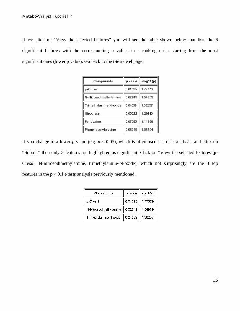
If we click on “View the selected features” you will see the table shown below that lists the 6

significant features with the corresponding p values in a ranking order starting from the most

significant ones (lower p value). Go back to the t-tests webpage.

If you change to a lower p value (e.g. p < 0.05), which is often used in t-tests analysis, and click on

“Submit” then only 3 features are highlighted as significant. Click on “View the selected features (p-

Cresol, N-nitrosodimethylamine, trimethylamine-N-oxide), which not surprisingly are the 3 top

features in the p < 0.1 t-tests analysis previously mentioned.

15


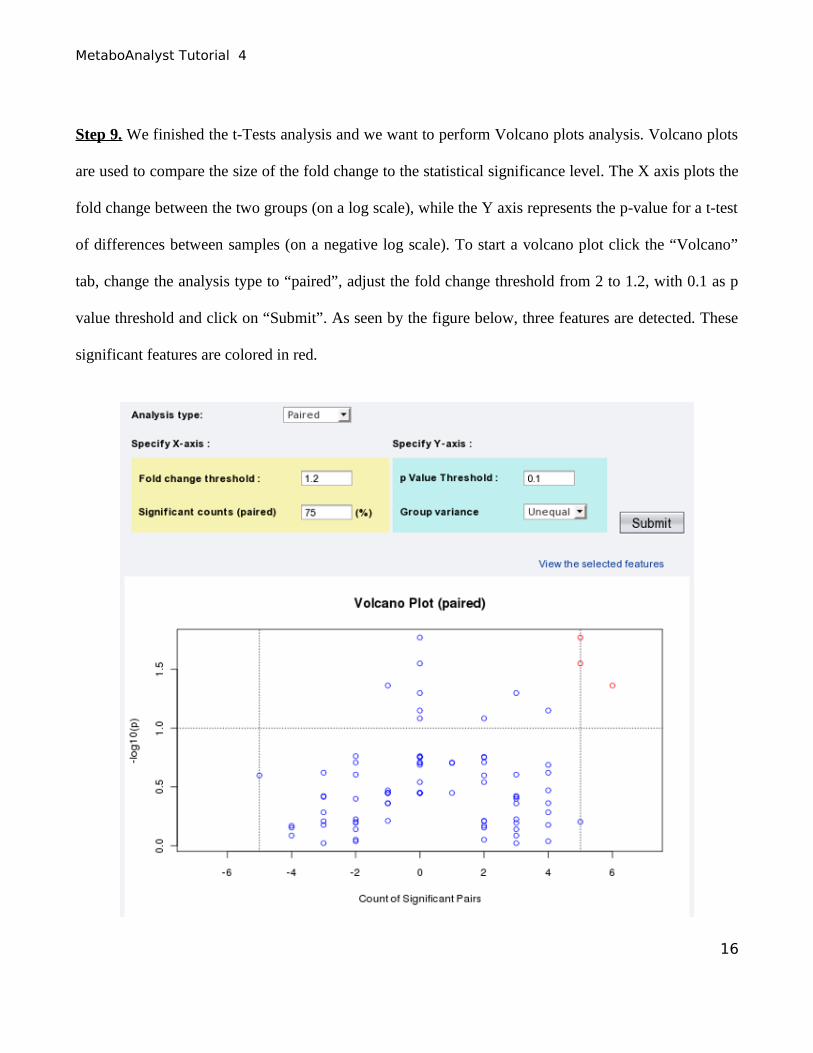
Step 9. We finished the t-Tests analysis and we want to perform Volcano plots analysis. Volcano plots

are used to compare the size of the fold change to the statistical significance level. The X axis plots the

fold change between the two groups (on a log scale), while the Y axis represents the p-value for a t-test

of differences between samples (on a negative log scale). To start a volcano plot click the “Volcano”

tab, change the analysis type to “paired”, adjust the fold change threshold from 2 to 1.2, with 0.1 as p

value threshold and click on “Submit”. As seen by the figure below, three features are detected. These

significant features are colored in red.

16


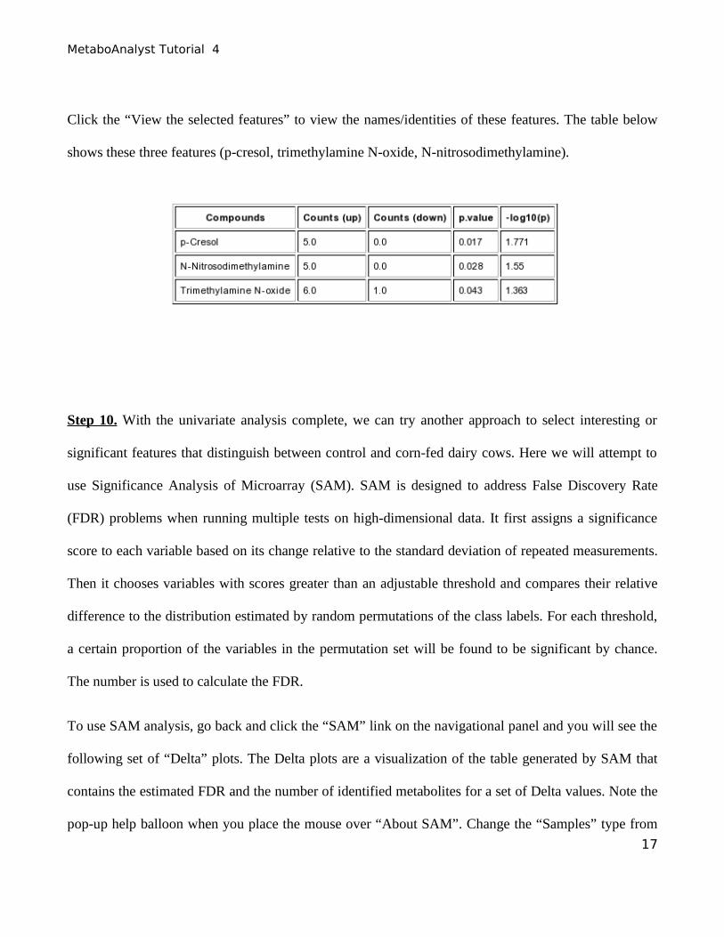
Click the “View the selected features” to view the names/identities of these features. The table below

shows these three features (p-cresol, trimethylamine N-oxide, N-nitrosodimethylamine).

Step 10. With the univariate analysis complete, we can try another approach to select interesting or

significant features that distinguish between control and corn-fed dairy cows. Here we will attempt to

use Significance Analysis of Microarray (SAM). SAM is designed to address False Discovery Rate

(FDR) problems when running multiple tests on high-dimensional data. It first assigns a significance

score to each variable based on its change relative to the standard deviation of repeated measurements.

Then it chooses variables with scores greater than an adjustable threshold and compares their relative

difference to the distribution estimated by random permutations of the class labels. For each threshold,

a certain proportion of the variables in the permutation set will be found to be significant by chance.

The number is used to calculate the FDR.

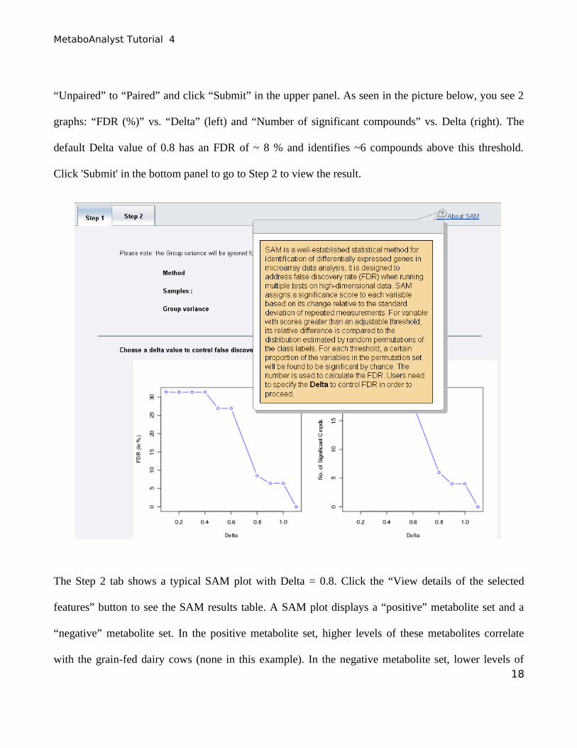
To use SAM analysis, go back and click the “SAM” link on the navigational panel and you will see the

following set of “Delta” plots. The Delta plots are a visualization of the table generated by SAM that

contains the estimated FDR and the number of identified metabolites for a set of Delta values. Note the

pop-up help balloon when you place the mouse over “About SAM”. Change the “Samples” type from

17


“Unpaired” to “Paired” and click “Submit” in the upper panel. As seen in the picture below, you see 2

graphs: “FDR (%)” vs. “Delta” (left) and “Number of significant compounds” vs. Delta (right). The

default Delta value of 0.8 has an FDR of ~ 8 % and identifies ~6 compounds above this threshold.

Click 'Submit' in the bottom panel to go to Step 2 to view the result.

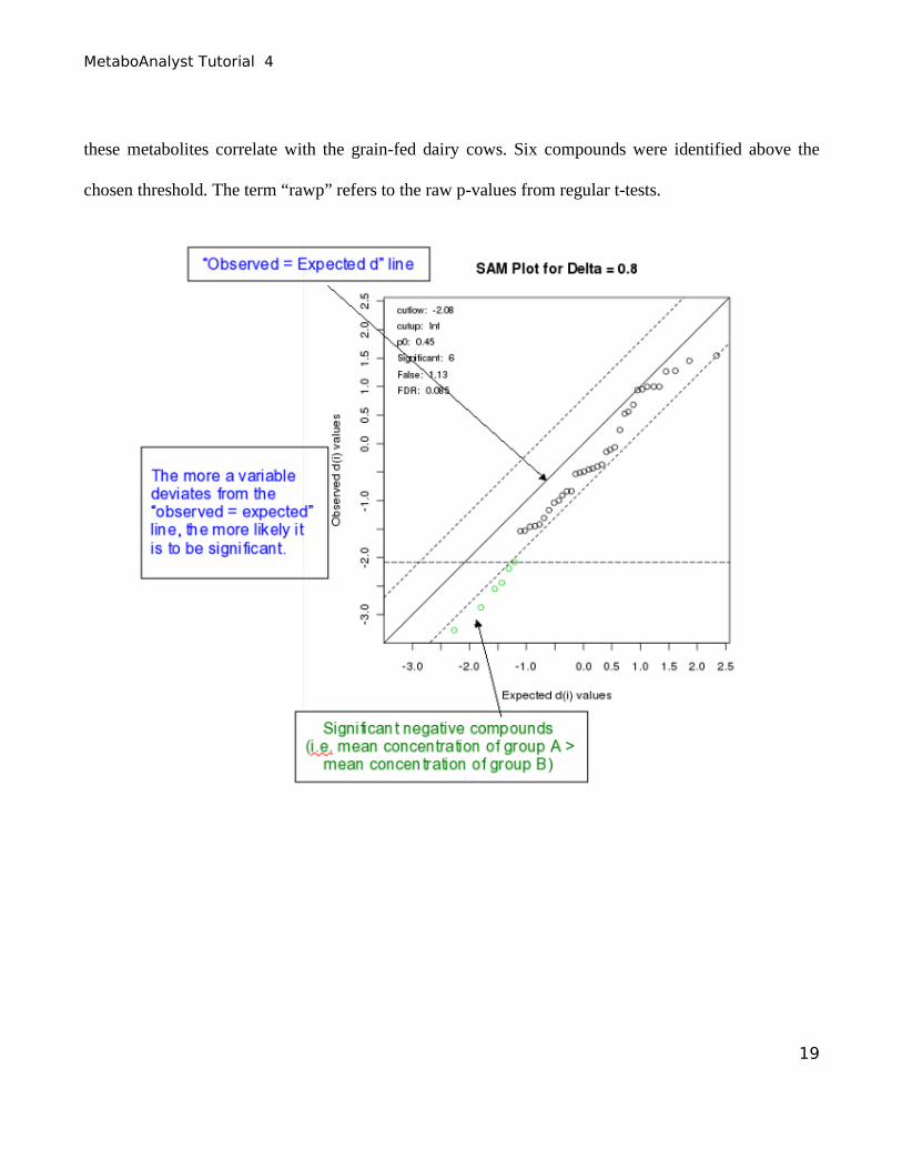
The Step 2 tab shows a typical SAM plot with Delta = 0.8. Click the “View details of the selected

features” button to see the SAM results table. A SAM plot displays a “positive” metabolite set and a

“negative” metabolite set. In the positive metabolite set, higher levels of these metabolites correlate

with the grain-fed dairy cows (none in this example). In the negative metabolite set, lower levels of 18


these metabolites correlate with the grain-fed dairy cows. Six compounds were identified above the

chosen threshold. The term “rawp” refers to the raw p-values from regular t-tests.

19


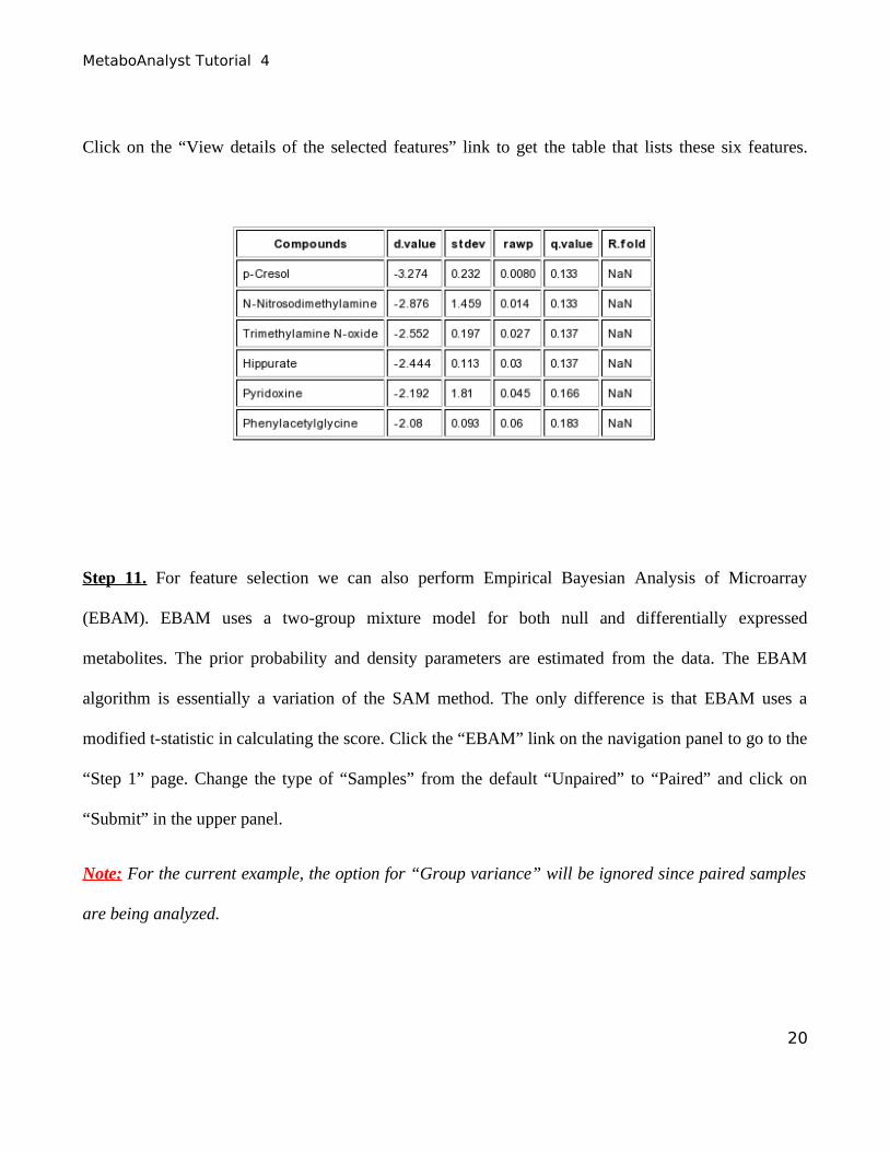
Click on the “View details of the selected features” link to get the table that lists these six features.

Step 11. For feature selection we can also perform Empirical Bayesian Analysis of Microarray

(EBAM). EBAM uses a two-group mixture model for both null and differentially expressed

metabolites. The prior probability and density parameters are estimated from the data. The EBAM

algorithm is essentially a variation of the SAM method. The only difference is that EBAM uses a

modified t-statistic in calculating the score. Click the “EBAM” link on the navigation panel to go to the

“Step 1” page. Change the type of “Samples” from the default “Unpaired” to “Paired” and click on

“Submit” in the upper panel.

Note: For the current example, the option for “Group variance” will be ignored since paired samples

are being analyzed.

20


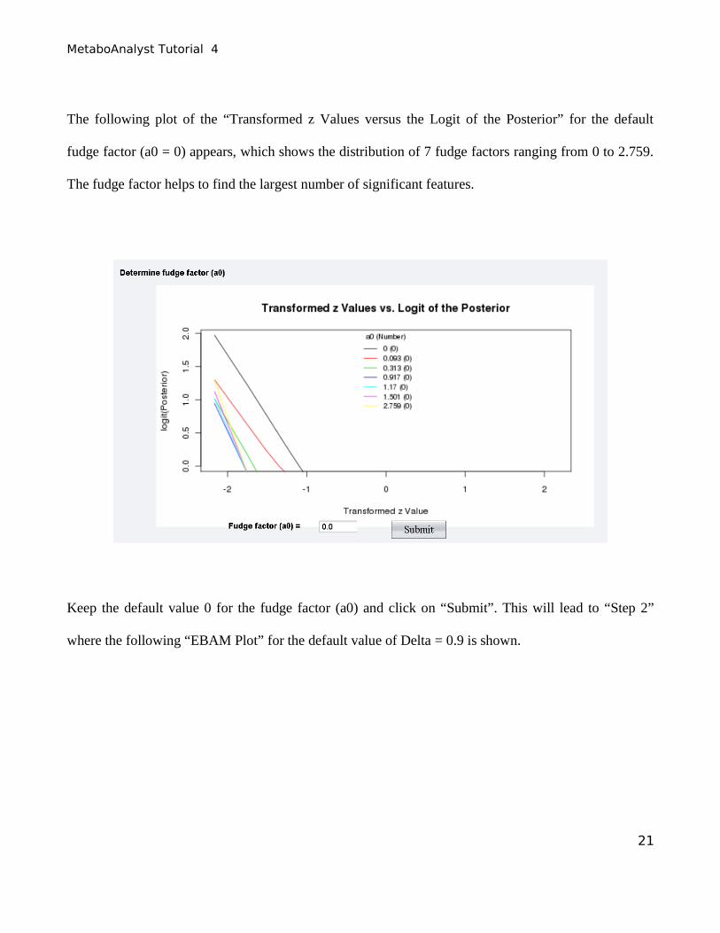
The following plot of the “Transformed z Values versus the Logit of the Posterior” for the default

fudge factor (a0 = 0) appears, which shows the distribution of 7 fudge factors ranging from 0 to 2.759.

The fudge factor helps to find the largest number of significant features.

Keep the default value 0 for the fudge factor (a0) and click on “Submit”. This will lead to “Step 2”

where the following “EBAM Plot” for the default value of Delta = 0.9 is shown.

21


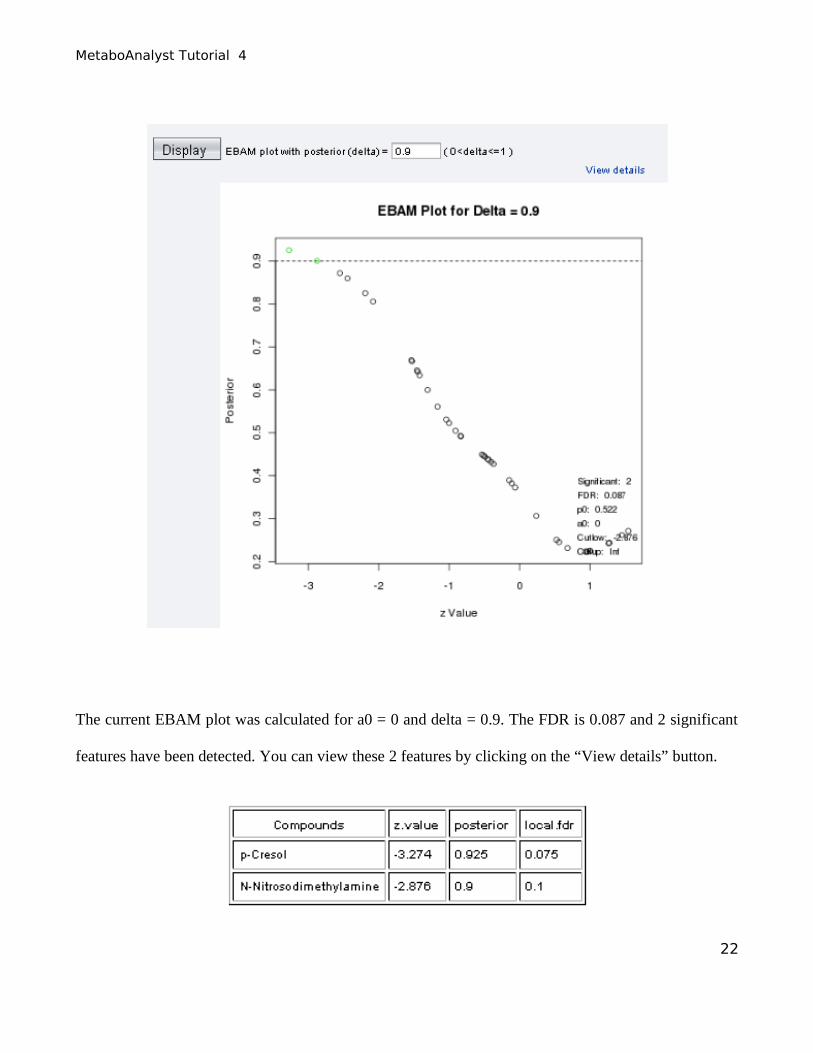
The current EBAM plot was calculated for a0 = 0 and delta = 0.9. The FDR is 0.087 and 2 significant

features have been detected. You can view these 2 features by clicking on the “View details” button.

22


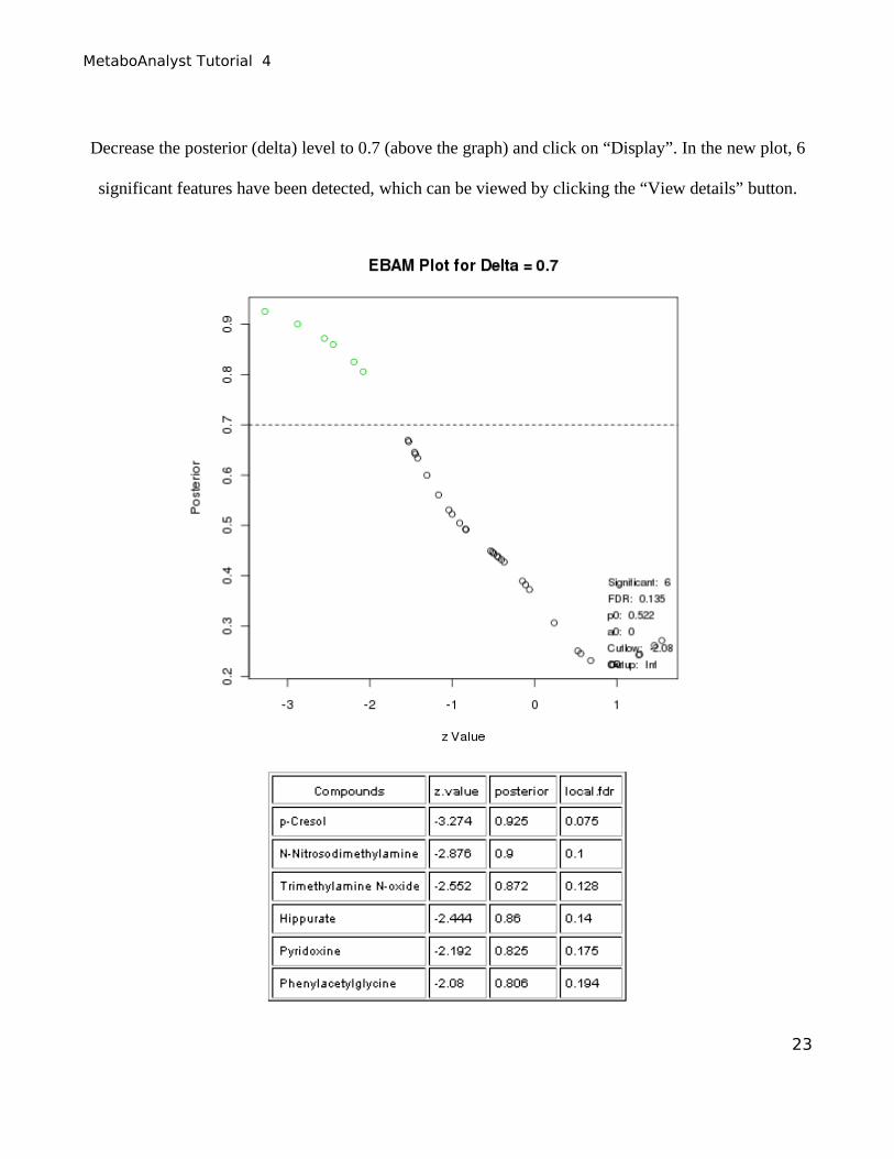
Decrease the posterior (delta) level to 0.7 (above the graph) and click on “Display”. In the new plot, 6

significant features have been detected, which can be viewed by clicking the “View details” button.

23


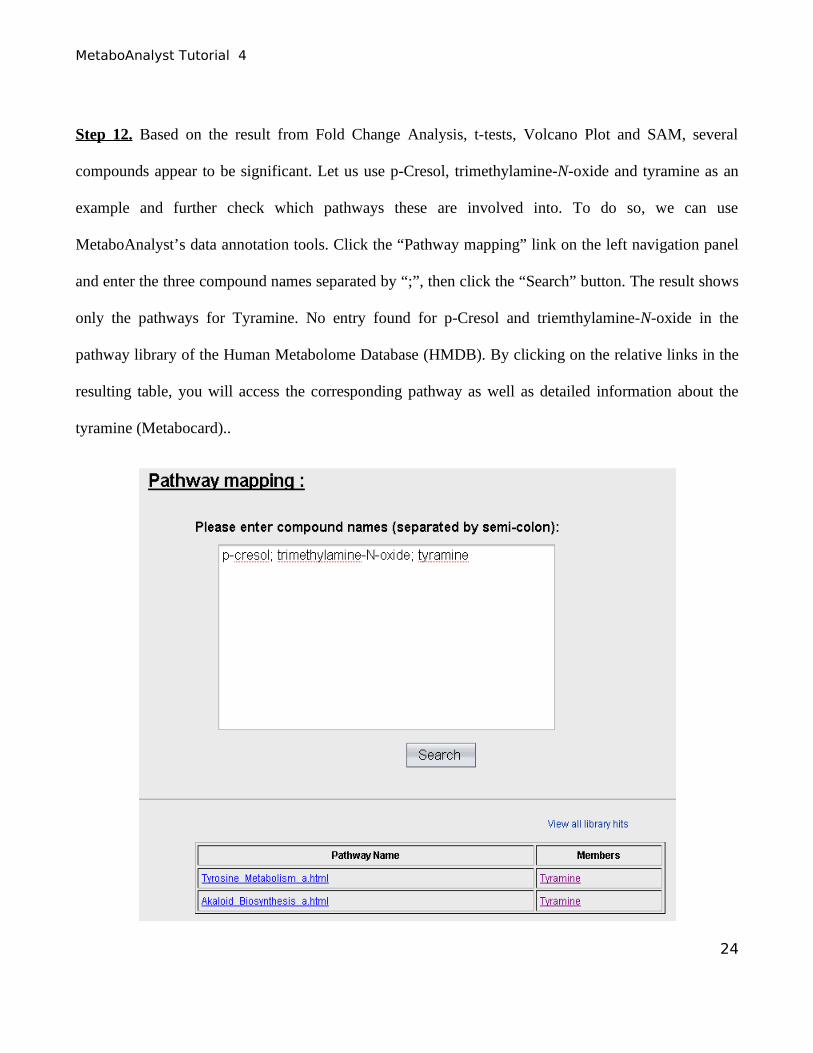
Step 12. Based on the result from Fold Change Analysis, t-tests, Volcano Plot and SAM, several

compounds appear to be significant. Let us use p-Cresol, trimethylamine-N-oxide and tyramine as an

example and further check which pathways these are involved into. To do so, we can use

MetaboAnalyst’s data annotation tools. Click the “Pathway mapping” link on the left navigation panel

and enter the three compound names separated by “;”, then click the “Search” button. The result shows

only the pathways for Tyramine. No entry found for p-Cresol and triemthylamine-N-oxide in the

pathway library of the Human Metabolome Database (HMDB). By clicking on the relative links in the

resulting table, you will access the corresponding pathway as well as detailed information about the

tyramine (Metabocard)..

24


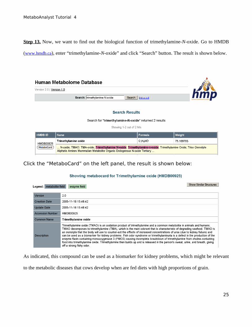
Step 13. Now, we want to find out the biological function of trimethylamine-N-oxide. Go to HMDB

(www.hmdb.ca), enter “trimethylamine-N-oxide” and click “Search” button. The result is shown below.

Click the “MetaboCard” on the left panel, the result is shown below:

As indicated, this compound can be used as a biomarker for kidney problems, which might be relevant

to the metabolic diseases that cows develop when are fed diets with high proportions of grain.

25

http://www.hmdb.ca/


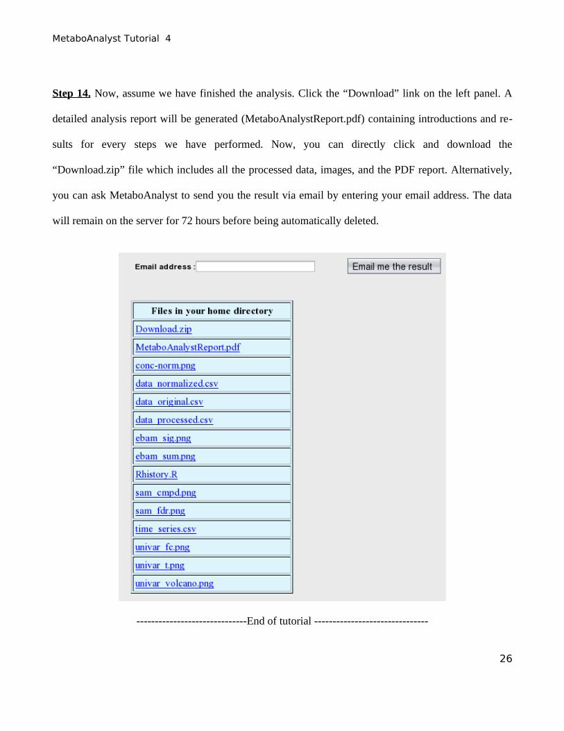
Step 14. Now, assume we have finished the analysis. Click the “Download” link on the left panel. A

detailed analysis report will be generated (MetaboAnalystReport.pdf) containing introductions and re-

sults for every steps we have performed. Now, you can directly click and download the

“Download.zip” file which includes all the processed data, images, and the PDF report. Alternatively,

you can ask MetaboAnalyst to send you the result via email by entering your email address. The data

will remain on the server for 72 hours before being automatically deleted.

------------------------------End of tutorial -------------------------------

26

Paired Analysis of Time-Series Studies Using Concentration ... · Paired Analysis of Time-Series...

Documents

Transcript of Paired Analysis of Time-Series Studies Using Concentration ... · Paired Analysis of Time-Series...