www.nr.no

Pair-copula constructions: even more flexible than copulas

Workshop on Copulas and Extremes

Grenoble, France, November 19th, 2013

Kjersti Aas Norwegian Computing Center

Joint work with: Claudia Czado, Ingrid Hobæk Haff, Arnoldo Frigessi, Daniel Berg, Eike C. Brechmann

www.nr.no

Pair-copula construction

► While there is a multitude of bivariate copula, the class of multivariate copulae is still quite restricted.

► Hence, if the dependency structures of different pairs of variables in a multivariate problem are very different, not even the copula approach will allow for the construction of an appropriate model.

► In this talk I will describe an extension to the state-of-the-art theory of copulas, modelling multivariate data using a so-called pair-copula construction.

www.nr.no

Copula► The Sklar’s theorem states that every multivariate

distribution F with marginals F1(x1),…,Fn(xn) can be written as

for some appropriate n-dimensional copula C.

► Using the chain rule, for an absolutely continuous joint distribution F with strictly increasing, continuous marginal distribution functions F1,…Fn it holds that

for some n-variate copula density .

www.nr.no

Pair-copula constructions (I)► For two random variables X1 and X2 we have

► Further, for three random variables X1, X2 and X3 we have

► It follows that for every j we have

www.nr.no

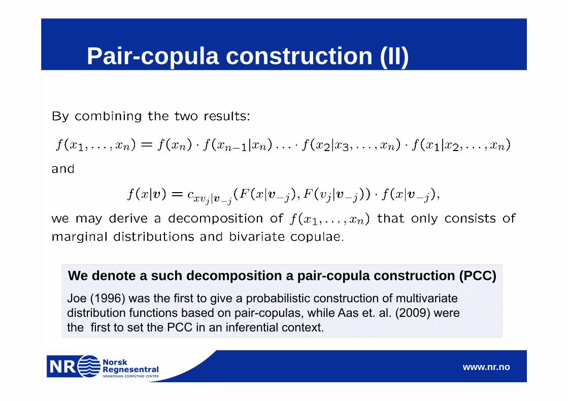
Pair-copula construction (II)

We denote a such decomposition a pair-copula construction (PCC)Joe (1996) was the first to give a probabilistic construction of multivariate distribution functions based on pair-copulas, while Aas et. al. (2009) were the first to set the PCC in an inferential context.

www.nr.no

PCC in three dimensions► A pair-copula construction of a three-dimensional

density is given by:

Special case: Trivariate normal distribution

If the marginal distributions are standard normal, and c12, c23and c13|2 are bivariate Gaussian copula densities, the resulting distribution is trivariate standard normal.

www.nr.no

PCC in five dimensions

► A possible pair-copula construction for a five-dimensional density is:

► There are as many as 480 different such constructions in the five-dimensional case, 23,040 in the 6-dimensional case and 2,580,480 in the 7-dimensional case......…..

www.nr.no

Vines► Hence, for high-dimensional distributions, there are a

significant number of possible pair-copula constructions.

► To help organising them, Bedford and Cooke (2001) introduced graphical models denoted regular vines (R-vines).

www.nr.no

Example in five dimensions

www.nr.no

Matrix representation

www.nr.no

Special case: C-vine

Each tree has a unique node that is connected to n-j edges.

f12345 = f1 · f2 · f3 · f4 · f5· c12 · c13 · c14 · c15· c23;1 · c24;1 · c25;1· c34;12 · c35;12· c45;123

Useful for ordering of importance

www.nr.no

Special case: D-vine No node in any tree is connected to more than two edges.

f1234 = f1 · f2 · f3 · f4 · f5· c12 · c23 · c34 · c45· c13;2 · c24;3 · c35;4· c14;23 · c25;34· c15;234

Useful for temporal ordering.

www.nr.no

General density expressions

www.nr.no

Conditional distribution functions

► The conditional distributions needed as copula arguments at level j are obtained as partial derivatives of the copulae at level j-1

► This is due to the following result of Joe (1996) stating that under regularity conditions we have:

The terms tree and level are used as synonyms in this talk

www.nr.no

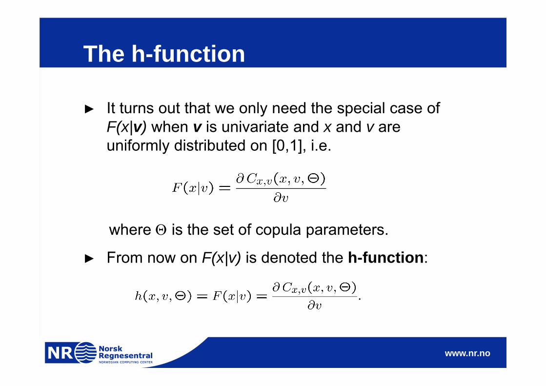
The h-function

► It turns out that we only need the special case of F(x|v) when v is univariate and x and v are uniformly distributed on [0,1], i.e.

where is the set of copula parameters.

► From now on F(x|v) is denoted the h-function:

www.nr.no

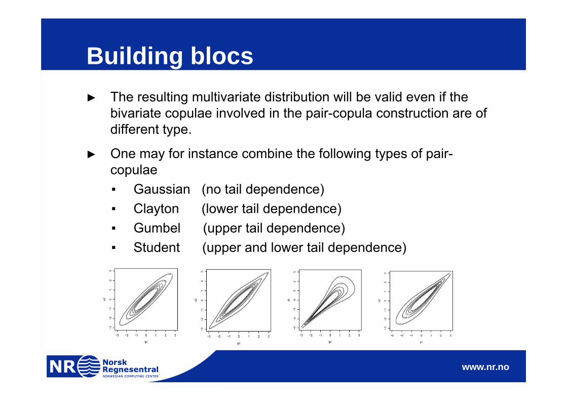
Building blocs► The resulting multivariate distribution will be valid even if the

bivariate copulae involved in the pair-copula construction are of different type.

► One may for instance combine the following types of pair-copulae▪ Gaussian (no tail dependence)▪ Clayton (lower tail dependence)▪ Gumbel (upper tail dependence)▪ Student (upper and lower tail dependence)

www.nr.no

Parameter estimation

www.nr.no

Three elements► Full inference for a pair-copula decomposition

should consider the following three tasks:

1. The selection of a specific factorisation.

2. The choice of pair-copula types.

3. The estimation of the parameters of the chosen pair-copulae.

www.nr.no

Which factorisation?

► The current idea is to capture the strongest pairwise dependencies in the first levels.

► Hence, for each tree we first calculate an empirical dependence measure (e.g. Kendall’s tau) for all variable pairs, and then we select the tree on all nodes that maximizes the sum of absolute empirical dependencies using the spanning tree algorithm of Prim.

www.nr.no

How does this look like for Tree 1?

www.nr.no

Choice of copula-types► The following procedure may be used to select copula types:

This procedure is also denoted sequential or stepwise semi-parametric estimation.

www.nr.no

ExamplecSM cMT cTB

cST|M cMB|T cSB|MT

Level I

Level IIILevel II

www.nr.no

Likelihood evaluation

www.nr.no

The SSP-estimator

► Full semi-parametric maximum likelihood estimation (SP) has shown to be consistent and asymptotically normal (Genest, 1995, Tsukahara, 2005).

► However, it is computationally too heavy in high dim.

► Hence, people tend to use the stepwise semi-parametric (SSP-) approach (Aas et. al., 2009) instead.

► In the SSP approach, the parameters of the vine are sequentially estimated starting from the top tree.

► The performance of SSP and SP is quite similar, but SSP is computationally much faster than SP.

www.nr.no

Properties of the SSP-estimator► Hobæk Haff (2011a) have shown that

▪ The SSP-estimator is less efficient than the SP-estimator in general.

▪ This loss of efficiency may however be rather low.▪ The SSP-estimator is semiparametrically efficient for

the Gaussian copula.

► Hobæk Haff (2011b) have shown that▪ The finite sample bias and MSE of SSP are higher

than those of SP (the difference increases with increasing dependency).

▪ With a small sample size or misspecification of the model, the difference between SP and SSP however becomes smaller.

www.nr.no

Simplifying assumption

► Generally, the parameters of the conditional density depends on the value of x2.

► Inference requires however the simplifying assumption that all pair copulae depend on the conditioning variables through the two conditional distribution functions that constitute their arguments only, and not directly.

► As shown in Hobæk Haff et. al. (2010), this seems not to be a severe restriction.

www.nr.no

Application:

Market risk model for the largest Norwegian bank, DNB

www.nr.no

Data set

► 19 financial variables that constitute the market portfolio of DNB.

► Daily log returns from March 2003 to March 2008 (1107 obs.) are used.

www.nr.no

Modelling procedure

► Fit appropriate ARMA-GARCH models for log-return time series.

► Fit an R-vine as well as a multivariate Student-t copula (for comparison) to standardized residuals

► Pair-copulas are selected from a range of 11 bivariate families using AIC: ▪ Independence copula, Gaussian, t, Clayton, rotated

Clayton (90°), Gumbel, rotated Gumbel (90°), Frank, Joe, Clayton-Gumbel (BB1), Joe-Clayton (BB7).

www.nr.no

First tree of R-vine

EUR3M

USD3M

NIBOR3M

Pengem.

Gov. bonds.

NIBOR5Y

HTM

Hedgefond

Int. stocks

No. stocks

FINX

Real estate

GBPEURYEN

USD

Int. bonds

USD5Y

EUR5Y

www.nr.no

Results

www.nr.no

Truncation (I)► The number of parameters in an R-vine grows

quadratically with the dimension.

► Hence, it would be useful to be able to reduce the model complexity.

► In Brechmann et. al (2012) we have studied the problem of determining whether an R-vine may be truncated.

► By a truncated R-vine at level K, we mean an R-vine with all pair-copulae with conditioning set larger than or equal to K set to independence copulae.

www.nr.no

► We fit one tree at a time and use the likelihood ratio test of Vuong (1989) to determine whether an additional tree provides a significant gain in the model fit.

Truncation (II)

www.nr.no

Truncation (III)

www.nr.no

Recent advances connected to PCC

www.nr.no

Applications► Finance

► Insurance

► Genetics

► Marketing

► Health

► Hydrology

► Infrastructure modeling

► Image analysis

www.nr.no

PCC types► Non-simplified PCC (Acar et. al., 2012).

► PCC with time-varying parameters (Almeida et. al., 2012, So & Yeung, 2013).

► Regime-switching PCC (Chollete et. al., 2008, Stӧber & Czado, 2013).

► Non-parametric PCC (Haff & Segers, 2013, Kauermann & Schellhase, 2013).

► Spatial PCC (Grӓler & Pebesma, 2011).

► PCC with discrete margins (Panagiotelis et. al., 2012).

► PCC for longitudinal data (Smith et. al., 2010).► PCC with Lévy copulas (Grothe & Nicklas, 2013).

www.nr.no

Summary

www.nr.no

Summary

► Pair-copula decomposed models represent a very flexible and intuitive way of constructing higher-dimensional copulae.

► Simulation and inference are straight-forward (but time-consuming in higher dimensions).

► Sequential and MLE parameter estimation of C-, D-and R-vines are available in R packages CDVineand VineCopula.