Page 1 Clock Synchronization: Physical Clocks Paul Krzyzanowski [email protected] [email protected]...
52
Page 1 Page 1 Clock Synchronization: Physical Clocks Paul Krzyzanowski [email protected] [email protected] Distributed Systems Except as otherwise noted, the content of this presentation is licensed under the Creative Commons Attribution 2.5 License.
-
Upload
allison-townsend -
Category
Documents
-
view
215 -
download
1
Transcript of Page 1 Clock Synchronization: Physical Clocks Paul Krzyzanowski [email protected] [email protected]...

Page 1Page 1
Clock Synchronization:Physical Clocks
Paul [email protected]
Distributed Systems
Except as otherwise noted, the content of this presentation is licensed under the Creative Commons Attribution 2.5 License.

Page 2
What’s it for?
• Temporal ordering of events produced by concurrent processes
• Synchronization between senders and receivers of messages
• Coordination of joint activity
• Serialization of concurrent access for shared objects

Page 3Page 3
Physical clocks

Page 4
Logical vs. physical clocks
Logical clock keeps track of event ordering– among related (causal) events
Physical clocks keep time of day– Consistent across systems

Page 5
Quartz clocks
• 1880: Piezoelectric effect– Curie brothers– Squeeze a quartz crystal & it generates an electric field– Apply an electric field and it bends
• 1929: Quartz crystal clock– Resonator shaped like tuning fork– Laser-trimmed to vibrate at 32,768 Hz– Standard resonators accurate to 6 parts per million at
31° C– Watch will gain/lose < ½ sec/day– Stability > accuracy: stable to 2 sec/month– Good resonator can have accuracy of 1 second in 10
years• Frequency changes with age, temperature, and acceleration

Page 6
Atomic clocks
• Second is defined as 9,192,631,770 periods of radiation corresponding to the transition between two hyperfine levels of cesium-133
• Accuracy:better than 1 second in six million years
• NIST standard since 1960

Page 7
UTC
• UT0– Mean solar time on Greenwich meridian– Obtained from astronomical observation
• UT1– UT0 corrected for polar motion
• UT2– UT1 corrected for seasonal variations in
Earth’s rotation
• UTC– Civil time measured on an atomic time scale
Page 8
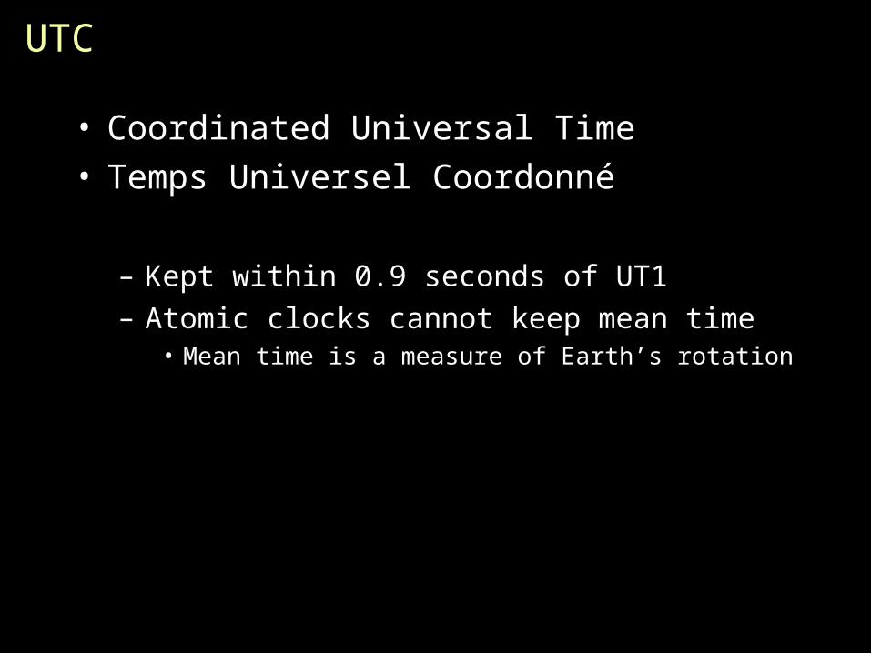
UTC
• Coordinated Universal Time• Temps Universel Coordonné
– Kept within 0.9 seconds of UT1– Atomic clocks cannot keep mean time
• Mean time is a measure of Earth’s rotation

Page 9
Physical clocks in computers
Real-time Clock: CMOS clock (counter) circuit driven by a quartz oscillator
– battery backup to continue measuring time when power is off
OS generally programs a timer circuit to generate an interrupt periodically
– e.g., 60, 100, 250, 1000 interrupts per second(Linux 2.6+ adjustable up to 1000 Hz)
– Programmable Interval Timer (PIT) – Intel 8253, 8254– Interrupt service procedure adds 1 to a counter in
memory

Page 10
Problem
Getting two systems to agree on time– Two clocks hardly ever agree– Quartz oscillators oscillate at slightly different
frequencies
Clocks tick at different rates– Create ever-widening gap in perceived time– Clock Drift
Difference between two clocks at one point in time– Clock Skew
Page 11
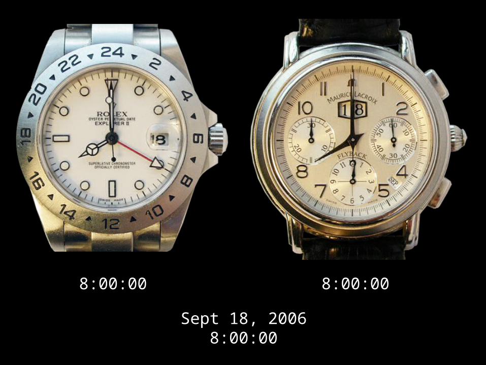
Sept 18, 20068:00:00
8:00:00 8:00:00

Page 12
Oct 23, 20068:00:00
8:01:24 8:01:48
Skew = +84 seconds+84 seconds/35 daysDrift = +2.4 sec/day
Skew = +108 seconds+108 seconds/35 daysDrift = +3.1 sec/day
Page 13
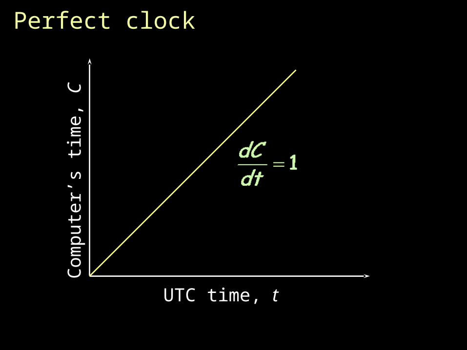
Perfect clock
UTC time, t
Com
pute
r’s
tim
e, C

Page 14
Drift with slow clock
UTC time, t
Com
pute
r’s
tim
e, C
skew

Page 15
Drift with fast clock
UTC time, t
Com
pute
r’s
tim
e, C
skew

Page 16
Dealing with drift
Assume we set computer to true time
Not good idea to set clock back– Illusion of time moving backwards can confuse
message ordering and software development environments

Page 17
Dealing with drift
Go for gradual clock correction
If fast:Make clock run slower until it synchronizes
If slow:Make clock run faster until it synchronizes
Page 18
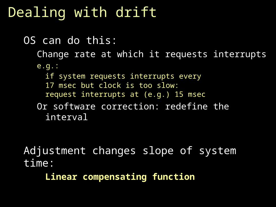
Dealing with drift
OS can do this:Change rate at which it requests interruptse.g.:
if system requests interrupts every17 msec but clock is too slow:
request interrupts at (e.g.) 15 msec
Or software correction: redefine the interval
Adjustment changes slope of system time:Linear compensating function

Page 19
Compensating for a fast clock
UTC time, t
Com
pute
r’s
tim
e, C
Linear compensatingfunction applied
Clock synchronizedskew

Page 20
Compensating for a fast clock
UTC time, t
Com
pute
r’s
tim
e, C

Page 21
Resynchronizing
After synchronization period is reached– Resynchronize periodically– Successive application of a second linear
compensating function can bring us closer to true slope
Keep track of adjustments and apply continuously
– e.g., UNIX adjtime system call

Page 22
Getting accurate time
• Attach GPS receiver to each computer± 1 msec of UTC
• Attach WWV radio receiverObtain time broadcasts from Boulder or DC± 3 msec of UTC (depending on distance)
• Attach GOES receiver± 0.1 msec of UTC
Not practical solution for every machine– Cost, size, convenience, environment

Page 23
Getting accurate time
Synchronize from another machine– One with a more accurate clock
Machine/service that provides time information:
Time server

Page 24
RPC
Simplest synchronization technique– Issue RPC to obtain time– Set time
Does not account for network or processing latency
client serverwhat’s the time?
3:42:19

Page 25
Cristian’s algorithm
Compensate for delays– Note times:
• request sent: T0
• reply received: T1
– Assume network delays are symmetric
server
clienttime
request reply
T0 T1
Tserver

Page 26
Cristian’s algorithm
Client sets time to:
server
clienttime
request reply
T0 T1
Tserver
= estimated overhead in each direction
Page 27
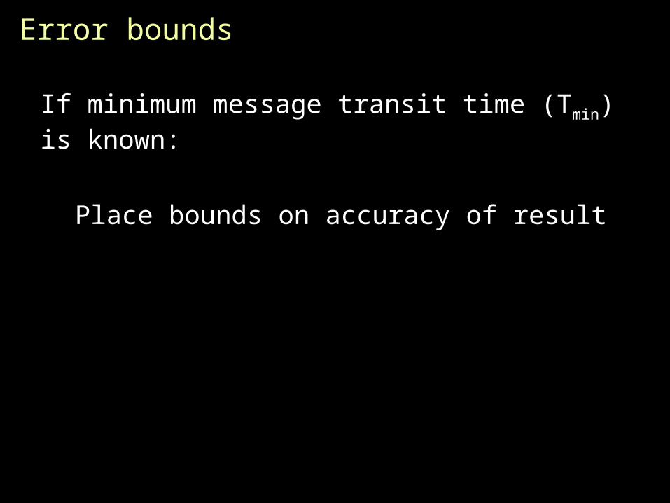
Error bounds
If minimum message transit time (Tmin) is known:
Place bounds on accuracy of result

Page 28
Error bounds
server
clienttime
request reply
T0 T1
Tserver
Tmin Tmin
Earliest time message arrives
Latest time message leaves
range = T1-T0-2Tmin
accuracy of result =

Page 29
Cristian’s algorithm: example
• Send request at 5:08:15.100 (T0)
• Receive response at 5:08:15.900 (T1)
– Response contains 5:09:25.300 (Tserver)
• Elapsed time is T1 -T0
5:08:15.900 - 5:08:15.100 = 800 msec
• Best guess: timestamp was generated400 msec ago
• Set time to Tserver+ elapsed time5:09:25.300 + 400 = 5:09.25.700

Page 30
Cristian’s algorithm: example
If best-case message time=200 msec
server
clienttime
request reply
T0 T1
Tserver
200 200
800
Error =
T0 = 5:08:15.100T1 = 5:08:15.900Ts = 5:09:25:300Tmin = 200msec

Page 31
Berkeley Algorithm
• Gusella & Zatti, 1989
• Assumes no machine has an accurate time source
• Obtains average from participating computers
• Synchronizes all clocks to average

Page 32
Berkeley Algorithm
• Machines run time dæmon– Process that implements protocol
• One machine is elected (or designated) as the server (master)– Others are slaves

Page 33
Berkeley Algorithm
• Master polls each machine periodically– Ask each machine for time
• Can use Cristian’s algorithm to compensate for network latency
• When results are in, compute average– Including master’s time
• Hope: average cancels out individual clock’s tendencies to run fast or slow
• Send offset by which each clock needs adjustment to each slave– Avoids problems with network delays if we
send a time stamp

Page 34
Berkeley Algorithm
Algorithm has provisions for ignoring readings from clocks whose skew is too great
– Compute a fault-tolerant average
If master fails– Any slave can take over

Page 35
Berkeley Algorithm: example
3:25 2:50 9:10
3:00
1. Request timestamps from all slaves
3:25
2:509:10
Page 36
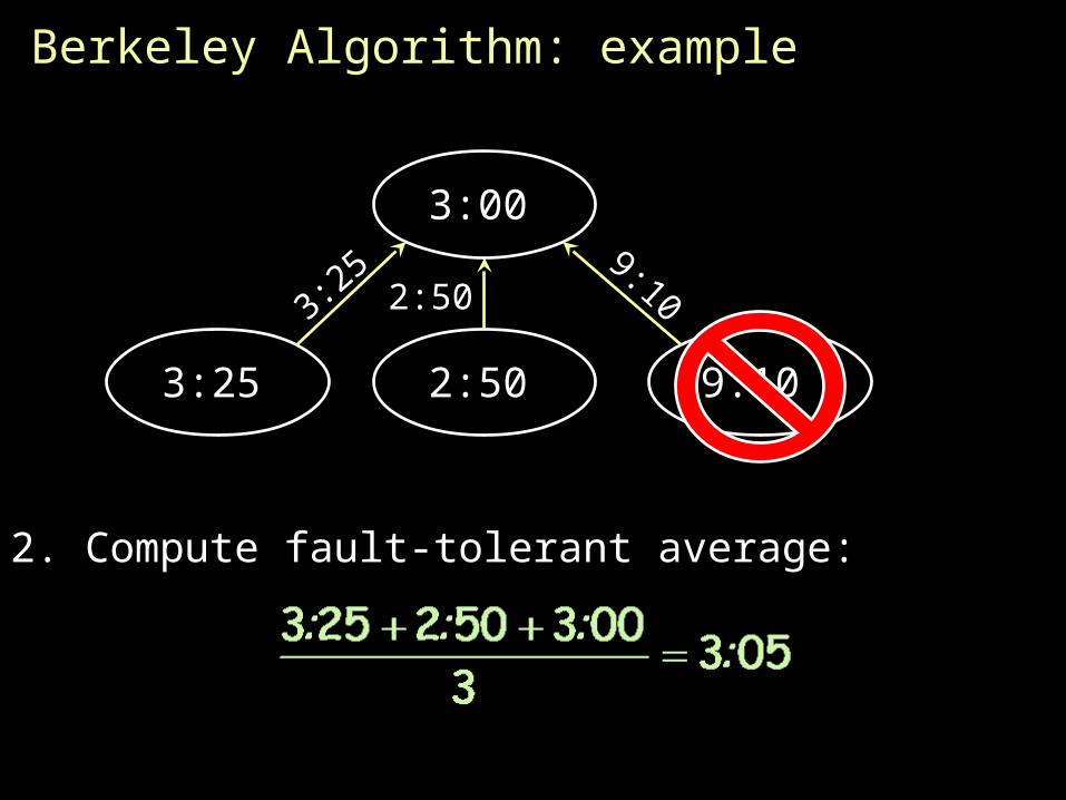
Berkeley Algorithm: example
3:25 2:50 9:10
3:00
2. Compute fault-tolerant average:
3:25
2:509:10

Page 37
Berkeley Algorithm: example
3:25 2:50 9:10
3:00
3. Send offset to each client
-0:2
0+0:15
-6:05
+0.15

Page 38
Network Time Protocol, NTP
1991, 1992Internet Standard, version 3: RFC 1305

Page 39
NTP Goals
• Enable clients across Internet to be accurately synchronized to UTC despite message delays– Use statistical techniques to filter data and gauge
quality of results
• Provide reliable service– Survive lengthy losses of connectivity– Redundant paths– Redundant servers
• Enable clients to synchronize frequently– offset effects of clock drift
• Provide protection against interference– Authenticate source of data

Page 40
NTP servers
Arranged in strata– 1st stratum: machines
connected directly to accurate time source
– 2nd stratum: machines synchronized from 1st stratum machines
– …
SYNCHRONIZATION SUBNET
1
2
3
4

Page 41
NTP Synchronization Modes
Multicast mode– for high speed LANS– Lower accuracy but efficient
Procedure call mode– Similar to Cristian’s algorithm
Symmetric mode– Intended for master servers– Pair of servers exchange messages and retain
data to improve synchronization over time
All messages delivered unreliably with UDP

Page 42
NTP messages
• Procedure call and symmetric mode– Messages exchanged in pairs
• NTP calculates:– Offset for each pair of messages
• Estimate of offset between two clocks
– Delay• Transmit time between two messages
– Filter Dispersion• Estimate of error – quality of results• Based on accuracy of server’s clock and consistency
of network transit time
• Use this data to find preferred server: – lower stratum & lowest total dispersion

Page 43
NTP message structure
• Leap second indicator– Last minute has 59, 60, 61 seconds
• Version number• Mode (symmetric, unicast, broadcast)• Stratum (1=primary reference, 2-15)• Poll interval
– Maximum interval between 2 successive messages, nearest power of 2
• Precision of local clock– Nearest power of 2

Page 44
NTP message structure
• Root delay– Total roundtrip delay to primary source– (16 bits seconds, 16 bits decimal)
• Root dispersion– Nominal error relative to primary source
• Reference clock ID– Atomic, NIST dial-up, radio, LORAN-C
navigation system, GOES, GPS, …
• Reference timestamp– Time at which clock was last set (64 bit)
• Authenticator (key ID, digest)– Signature (ignored in SNTP)

Page 45
NTP message structure
• T1: originate timestamp– Time request departed client (client’s time)
• T2: receive timestamp– Time request arrived at server (server’s time)
• T3: transmit timestamp– Time request left server (server’s time)

Page 46
NTP’s validation tests
• Timestamp provided ≠ last timestamp received– duplicate message?
• Originating timestamp in message consistent with sent data– Messages arriving in order?
• Timestamp within range?• Originating and received timestamps ≠ 0?• Authentication disabled? Else authenticate• Peer clock is synchronized?• Don’t sync with clock of higher stratum #• Reasonable data for delay & dispersion

Page 47
SNTP
Simple Network Time Protocol– Based on Unicast mode of NTP– Subset of NTP, not new protocol– Operates in multicast or procedure call mode– Recommended for environments where server
is root node and client is leaf of synchronization subnet
– Root delay, root dispersion, reference timestamp ignored
RFC 2030, October 1996

Page 48
SNTP
Roundtrip delay:
d = (T4-T1) - (T2-T3)
server
clienttime
request reply
T1
T2
T4
T3
Time offset:
Page 49
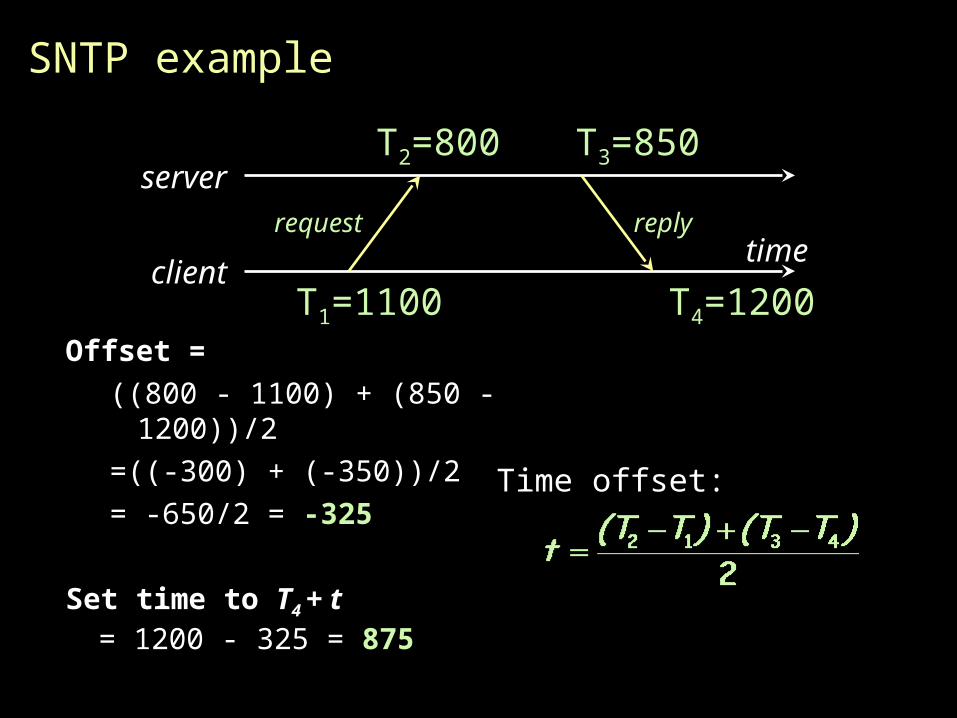
SNTP example
server
clienttime
request reply
T1=1100
T2=800
T4=1200
T3=850
Time offset:
Offset = ((800 - 1100) + (850 - 1200))/2=((-300) + (-350))/2= -650/2 = -325
Set time to T4 + t= 1200 - 325 = 875

Page 50
Cristian’s algorithm
server
clienttime
request reply
T1=1100
T2=800
T4=1200
T3=850
Offset = (1200 - 1100)/2 = 50
Set time to Ts + offset= 825 + 50 = 875
Ts=825

Page 51
Key Points: Physical Clocks
• Cristian’s algorithm & SNTP– Set clock from server– But account for network delays– Error: uncertainty due to network/processor
latency: errors are additive±10 msec and ±20 msec = ±30 msec.
• Adjust for local clock skew– Linear compensating function

Page 52Page 52
The end.