ISSN 1594­1906

Padova and Asiago Observatories

Technical Report n. 24

February 2010

Document available at: http://www.pd.astro.it/

Vicolo dell’Osservatorio, 5  35122 Padova – Tel. +390498293411 – Fax +390418759840

A simple method for reduction of  Echelle spectra by IRAF

T. Iijima

ISSN 1594­1906

A simple method for reduction of echelle spectra by IRAF1

Takashi IIJIMA

Astronomical Observatory of Padova, Asiago Station

prefaceThis manual presents a simple and easy method to reduce spectra of stellar or compact objects obtained with the Reosc Echelle spectrograph mounted on the 182 cm telescope at the Mount Ekar station of the Astronomical Observatory of Padova. The calibrations of the sensitivity of the spectrograph are made using the spectra of standard stars obtained in the same nights of the observations. The author uses a cross disperser of 300 lines mm¯¹. When the other cross dispersers are used (150 lines mm¯¹ and 1200 lines mm¯¹ are also available), some parameters should be changed.Appendix gives an introduction for IRAF beginners.

1:IRAF is distributed by NOAO for Research in Astronomy, Inc. under cooperative agreement with the National Science Foundation.

ISSN 1594­1906

1. Observations.

First of all the author suggests the observers to obtain spectra with high S/N ratio, because the reductions of faint spectra are very difficult. A secret path for reduction of faint spectra is presented later (Section 3.3).Uncompleted orders can not be reduced by our method,

because in such a case a divide by zero operation occurs in the calibration pipeline. Thus, the observers have to make complete the orders of interest adjusting the angle of the grating.The calibrations of the sensitivity of the spectrograph are

made using the spectra of standard stars obtained in the same night of the observation. To this aim it is necessary to obtain spectra of standard stars located in the vicinity of the objects or at least with similar airmass. A list of the standard stars available in IRAF can be obtained with the command:cl> page onedstds$README

The bright standard stars reported in the directories onedstds$spec16cal/ and onedstds$irscal/ are adequate for our method.Figure 1 shows an image of a spectrum obtained with our

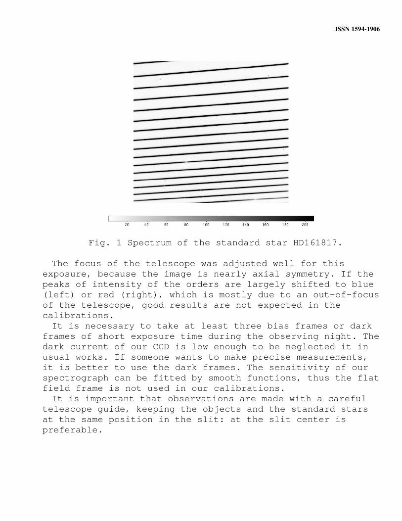
spectrograph. The cross disperser 300 lines mm¯¹ is used and the grating angle is set to -9°20'. The object is the standard star HD161817 and the exposure time is 600 sec. The spectrum covers the range from 4350 to 6100Å with a resolution of R=10000.

ISSN 1594­1906

Fig. 1 Spectrum of the standard star HD161817.

The focus of the telescope was adjusted well for this exposure, because the image is nearly axial symmetry. If the peaks of intensity of the orders are largely shifted to blue (left) or red (right), which is mostly due to an out-of-focus of the telescope, good results are not expected in the calibrations.It is necessary to take at least three bias frames or dark

frames of short exposure time during the observing night. The dark current of our CCD is low enough to be neglected it in usual works. If someone wants to make precise measurements, it is better to use the dark frames. The sensitivity of our spectrograph can be fitted by smooth functions, thus the flat field frame is not used in our calibrations.It is important that observations are made with a careful

telescope guide, keeping the objects and the standard stars at the same position in the slit: at the slit center is preferable.

ISSN 1594­1906

2. Preparation.

Before to start with the reductions of the spectra, some processing is required on the original images using the commands in the directory images.The format of the original images obtained by the Reosc

Echelle spectrograph is fits, but with names of the kind IMA***.FTS. The extension of file name processed in IRAF has to be fits, so that the file names must be accordingly changed out of IRAF, e.g., in Linux.$mv IMA***.FTS ima***.fits

To proceed it is necessary to cut away the margins of the images using the command imcopy.im>imcopy (name of image)[x1:x2,y1:y2] (name of trimmed image)

where x1,x2,y1,y2 are the limits at left, right, bottom, and top of the image, respectively. The author uses the values [11:1064,2:1050]. The wildcards are useful when many images are processed. For example, to trim all images with names starting by eim, giving them new names starting by fim the command is:im> imcopy eim*[x1:x2,y1:y2] %eim%fim%*.*

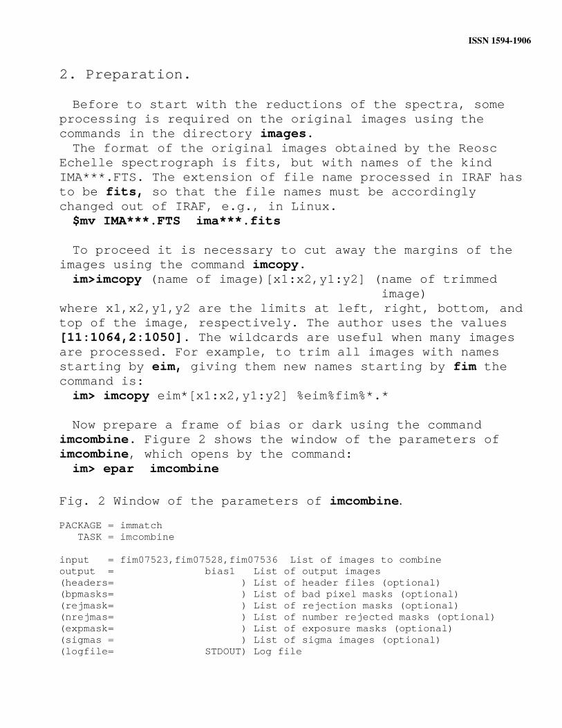
Now prepare a frame of bias or dark using the command imcombine. Figure 2 shows the window of the parameters of imcombine, which opens by the command:im> epar imcombine

Fig. 2 Window of the parameters of imcombine.

PACKAGE = immatch TASK = imcombine

input = fim07523,fim07528,fim07536 List of images to combineoutput = bias1 List of output images(headers= ) List of header files (optional)(bpmasks= ) List of bad pixel masks (optional)(rejmask= ) List of rejection masks (optional)(nrejmas= ) List of number rejected masks (optional)(expmask= ) List of exposure masks (optional)(sigmas = ) List of sigma images (optional)(logfile= STDOUT) Log file

ISSN 1594­1906

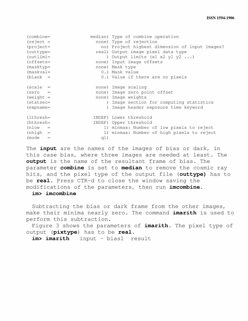
(combine= median) Type of combine operation(reject = none) Type of rejection(project= no) Project highest dimension of input images?(outtype= real) Output image pixel data type(outlimi= ) Output limits (x1 x2 y1 y2 ...)(offsets= none) Input image offsets(masktyp= none) Mask type(maskval= 0.) Mask value(blank = 0.) Value if there are no pixels

(scale = none) Image scaling(zero = none) Image zero point offset(weight = none) Image weights(statsec= ) Image section for computing statistics(expname= ) Image header exposure time keyword

(lthresh= INDEF) Lower threshold(hthresh= INDEF) Upper threshold(nlow = 1) minmax: Number of low pixels to reject(nhigh = 1) minmax: Number of high pixels to reject(mode = ql)

The input are the names of the images of bias or dark, in this case bias, where three images are needed at least. The output is the name of the resultant frame of bias. The parameter combine is set to median to remove the cosmic ray hits, and the pixel type of the output file (outtype) has to be real. Press CTR-d to close the window saving the modifications of the parameters, then run imcombine.im> imcombine

Subtracting the bias or dark frame from the other images, make their minima nearly zero. The command imarith is used to perform this subtraction.Figure 3 shows the parameters of imarith. The pixel type of

output (pixtype) has to be real.im> imarith input – bias1 result

ISSN 1594­1906

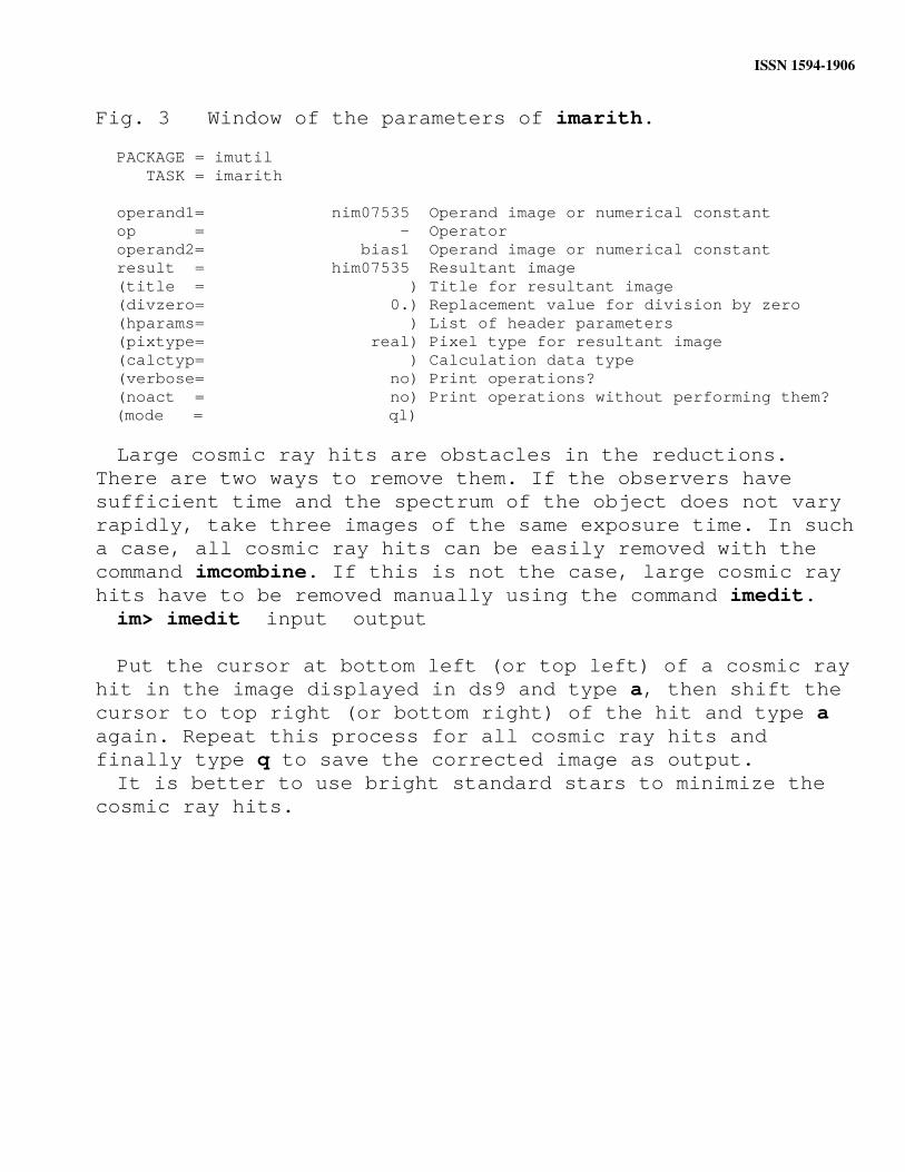
Fig. 3 Window of the parameters of imarith.

PACKAGE = imutil TASK = imarith

operand1= nim07535 Operand image or numerical constant op = - Operatoroperand2= bias1 Operand image or numerical constantresult = him07535 Resultant image(title = ) Title for resultant image(divzero= 0.) Replacement value for division by zero(hparams= ) List of header parameters(pixtype= real) Pixel type for resultant image(calctyp= ) Calculation data type(verbose= no) Print operations?(noact = no) Print operations without performing them?

(mode = ql)

Large cosmic ray hits are obstacles in the reductions. There are two ways to remove them. If the observers have sufficient time and the spectrum of the object does not vary rapidly, take three images of the same exposure time. In such a case, all cosmic ray hits can be easily removed with the command imcombine. If this is not the case, large cosmic ray hits have to be removed manually using the command imedit. im> imedit input output

Put the cursor at bottom left (or top left) of a cosmic ray hit in the image displayed in ds9 and type a, then shift the cursor to top right (or bottom right) of the hit and type a again. Repeat this process for all cosmic ray hits and finally type q to save the corrected image as output.It is better to use bright standard stars to minimize the

cosmic ray hits.

ISSN 1594­1906

3. Extractions of orders of spectra.

3.1. Spectra of bright objects.

In this section we discuss the process for the extraction of the orders of spectra. The commands in the directory echelle are used. The path to the directory echelle iscl> noao> imred > echelle

Prior to the beginning of a new work, it is better to remove all old ap-files in the folder of database, because sometimes the old ap-files become obstacles in the reductions, for example if the same name of the image was used for a different image in an earlier work. This process is made out of IRAF with the command of Linux.$ rm ap*

The direction of the spectral dispersion of our spectro-graph is horizontal as seen in Fig. 1, while that in the default setting of IRAF is vertical. Thus, the parameter of the dispersion axis (dispaxi) has to be changed as 1, with the command:ec> epar echelle

Here we try to extract the orders of the spectrum of the standard star HD161817 shown in Fig. 1 as an example. The command apall is used. Since there are so many parameters in apall, the window has to be extended maximum. The window of the parameters of apall is shown in Fig. 4 which opens with the command: ec> epar apall

The input is the name of the image of the spectrum and the output is the name of the destination file in which the extracted one-dimensional tracings of the orders will be saved. All parameters from interac to review can be yes. The author feels that more beautiful tracings are extracted with resize = no, but this is his personal liking.

ISSN 1594­1906

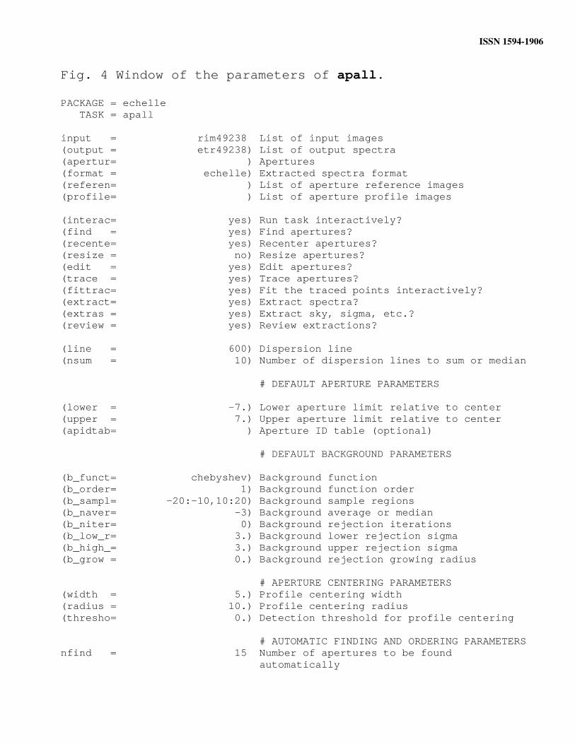
Fig. 4 Window of the parameters of apall.

PACKAGE = echelle TASK = apall

input = rim49238 List of input images(output = etr49238) List of output spectra(apertur= ) Apertures(format = echelle) Extracted spectra format(referen= ) List of aperture reference images(profile= ) List of aperture profile images

(interac= yes) Run task interactively?(find = yes) Find apertures?(recente= yes) Recenter apertures?(resize = no) Resize apertures?(edit = yes) Edit apertures?(trace = yes) Trace apertures?(fittrac= yes) Fit the traced points interactively?(extract= yes) Extract spectra?(extras = yes) Extract sky, sigma, etc.?(review = yes) Review extractions?

(line = 600) Dispersion line(nsum = 10) Number of dispersion lines to sum or median

# DEFAULT APERTURE PARAMETERS

(lower = -7.) Lower aperture limit relative to center(upper = 7.) Upper aperture limit relative to center(apidtab= ) Aperture ID table (optional)

# DEFAULT BACKGROUND PARAMETERS

(b_funct= chebyshev) Background function(b_order= 1) Background function order(b_sampl= -20:-10,10:20) Background sample regions(b_naver= -3) Background average or median(b_niter= 0) Background rejection iterations(b_low_r= 3.) Background lower rejection sigma(b_high_= 3.) Background upper rejection sigma(b_grow = 0.) Background rejection growing radius

# APERTURE CENTERING PARAMETERS(width = 5.) Profile centering width(radius = 10.) Profile centering radius(thresho= 0.) Detection threshold for profile centering

# AUTOMATIC FINDING AND ORDERING PARAMETERSnfind = 15 Number of apertures to be found automatically

ISSN 1594­1906

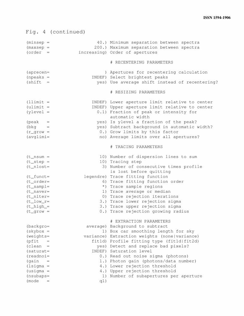
Fig. 4 (continued)

(minsep = 40.) Minimum separation between spectra(maxsep = 200.) Maximum separation between spectra(order = increasing) Order of apertures

# RECENTERING PARAMETERS

(aprecen= ) Apertures for recentering calculation(npeaks = INDEF) Select brightest peaks(shift = yes) Use average shift instead of recentering?

# RESIZING PARAMETERS

(llimit = INDEF) Lower aperture limit relative to center(ulimit = INDEF) Upper aperture limit relative to center(ylevel = 0.1) Fraction of peak or intensity for automatic width(peak = yes) Is ylevel a fraction of the peak?(bkg = yes) Subtract background in automatic width?(r_grow = 0.) Grow limits by this factor(avglimi= no) Average limits over all apertures?

# TRACING PARAMETERS

(t_nsum = 10) Number of dispersion lines to sum(t_step = 10) Tracing step(t_nlost= 3) Number of consecutive times profile is lost before quitting (t_funct= legendre) Trace fitting function(t_order= 6) Trace fitting function order(t_sampl= *) Trace sample regions(t_naver= 1) Trace average or median(t_niter= 0) Trace rejection iterations(t_low_r= 3.) Trace lower rejection sigma(t_high_= 3.) Trace upper rejection sigma(t_grow = 0.) Trace rejection growing radius

# EXTRACTION PARAMETERS(backgro= average) Background to subtract(skybox = 1) Box car smoothing length for sky(weights= variance) Extraction weights (none|variance)(pfit = fit1d) Profile fitting type (fit1d|fit2d)(clean = yes) Detect and replace bad pixels?(saturat= INDEF) Saturation level(readnoi= 0.) Read out noise sigma (photons)(gain = 1.) Photon gain (photons/data number)(lsigma = 4.) Lower rejection threshold(usigma = 4.) Upper rejection threshold(nsubaps= 1) Number of subapertures per aperture(mode = ql)

ISSN 1594­1906

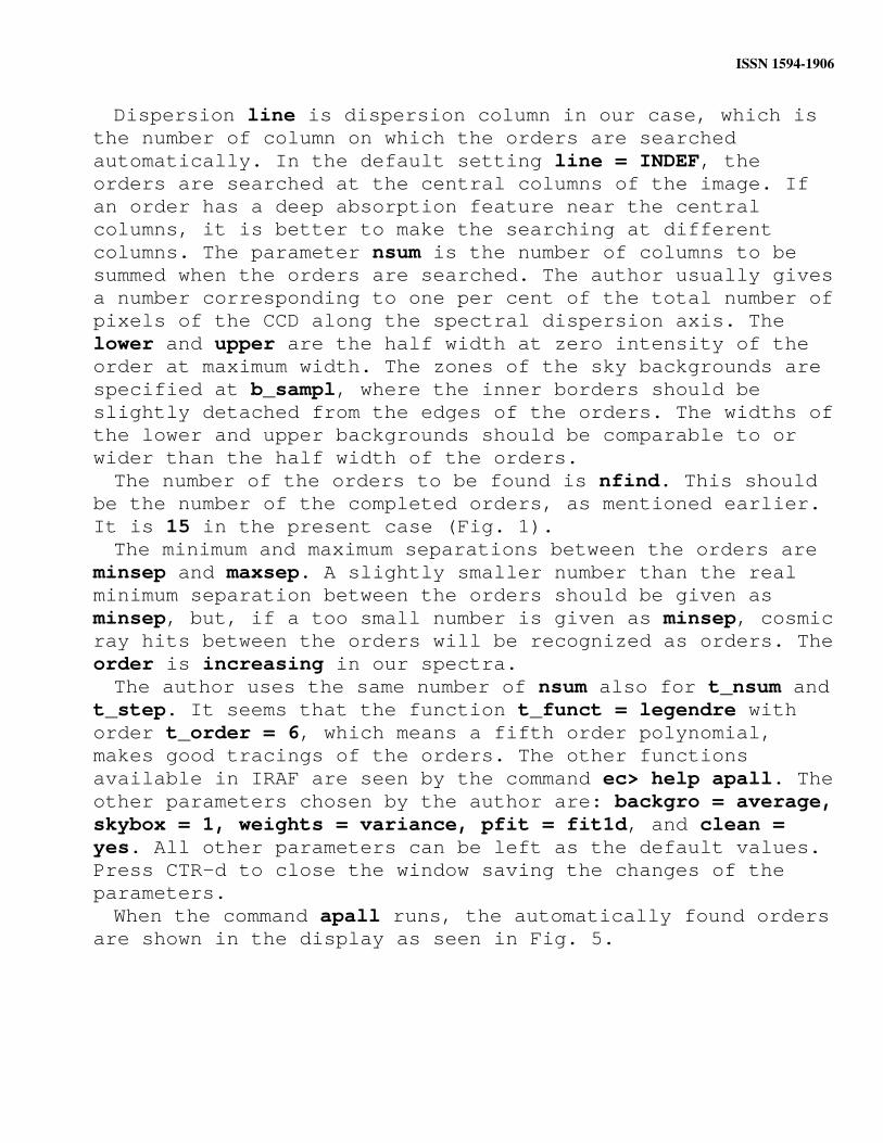
Dispersion line is dispersion column in our case, which is the number of column on which the orders are searched automatically. In the default setting line = INDEF, the orders are searched at the central columns of the image. If an order has a deep absorption feature near the central columns, it is better to make the searching at different columns. The parameter nsum is the number of columns to be summed when the orders are searched. The author usually gives a number corresponding to one per cent of the total number of pixels of the CCD along the spectral dispersion axis. The lower and upper are the half width at zero intensity of the order at maximum width. The zones of the sky backgrounds are specified at b_sampl, where the inner borders should be slightly detached from the edges of the orders. The widths of the lower and upper backgrounds should be comparable to or wider than the half width of the orders.The number of the orders to be found is nfind. This should

be the number of the completed orders, as mentioned earlier. It is 15 in the present case (Fig. 1). The minimum and maximum separations between the orders are

minsep and maxsep. A slightly smaller number than the real minimum separation between the orders should be given as minsep, but, if a too small number is given as minsep, cosmic ray hits between the orders will be recognized as orders. The order is increasing in our spectra.The author uses the same number of nsum also for t_nsum and

t_step. It seems that the function t_funct = legendre with order t_order = 6, which means a fifth order polynomial, makes good tracings of the orders. The other functions available in IRAF are seen by the command ec> help apall. The other parameters chosen by the author are: backgro = average, skybox = 1, weights = variance, pfit = fit1d, and clean = yes. All other parameters can be left as the default values. Press CTR-d to close the window saving the changes of the parameters.When the command apall runs, the automatically found orders

are shown in the display as seen in Fig. 5.

ISSN 1594­1906

Fig. 5 Automatically found orders.

When a faint spectrum is reduced, sometimes mis-identifications of the orders occur. In such a case, put the cross on the point of the wrong identification and type d to delete the mark, then put the cross on the true order and

Fig. 6 Locus of an order.

ISSN 1594­1906

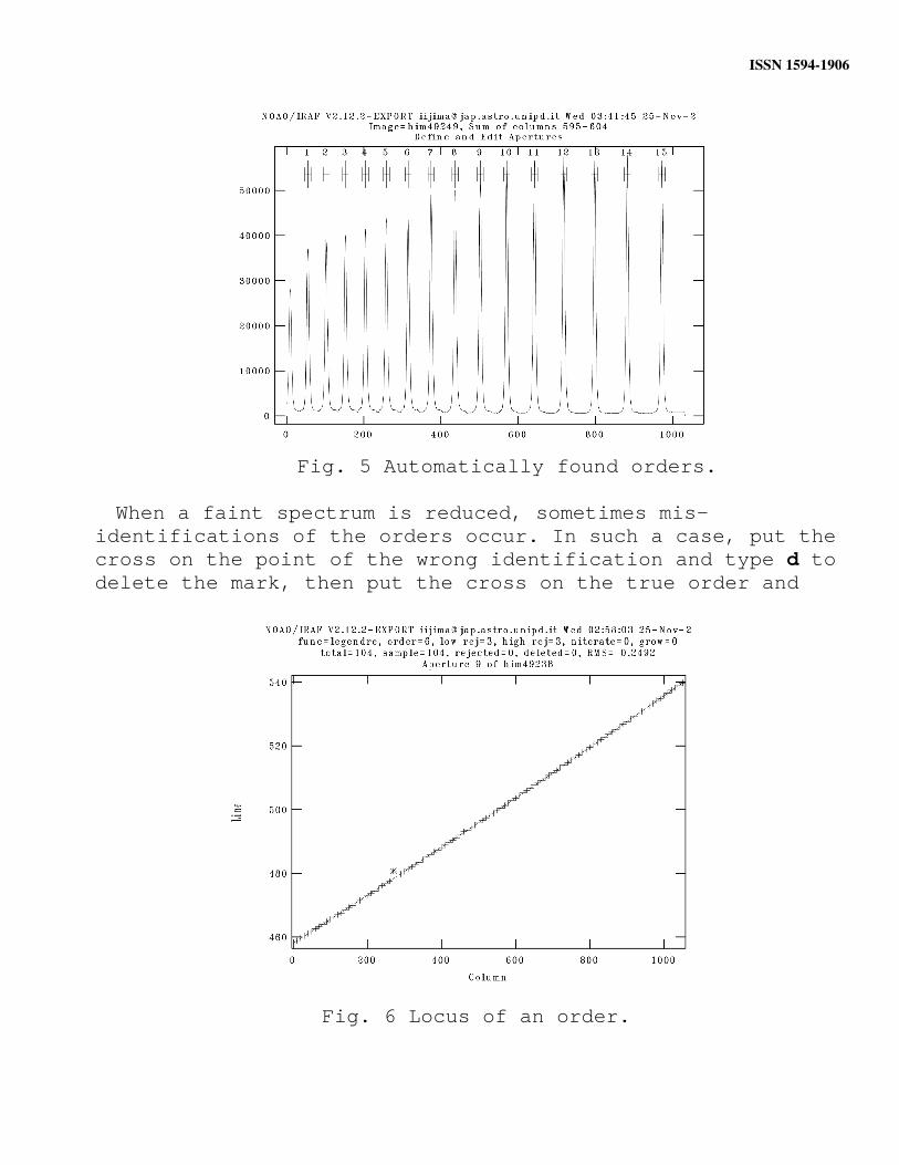
type m to mark it. When all orders are marked correctly, type q and answer yes the successive questions. The locus of the first order and the fitting curve appear in the display as seen in Fig. 6.Sometimes points detached from the locus appear, which are

mainly due to nearby cosmic ray hits. In such a case, put the cross on the point and type d to delete it, then type f to make the new fitting. The asterisk in Fig. 6 is a deleted point. When the order is traced well, type q and answer yes the question. The locus of the next order will appear. When a very faint spectrum is reduced, sometimes the locus

of the order is lost, and appears a figure such as Fig. 7.

Fig. 7 A failure of the tracing of an order.

In such a case, the process should be interrupted and a new attempt must be done with different parameters (see, Section 3.3). When the loci of all orders are traced well, answer yes the successive questions. If the process was interrupted, answer no the final questions in order to try again with new parameters.If the questions have been answered yes, the tracings of

the orders appear on the display one by one, as seen in Fig. 8.

ISSN 1594­1906

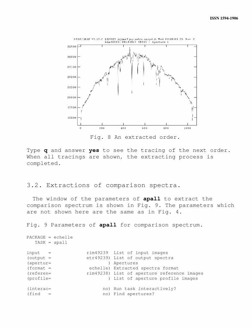
Fig. 8 An extracted order.

Type q and answer yes to see the tracing of the next order. When all tracings are shown, the extracting process is completed.

3.2. Extractions of comparison spectra.

The window of the parameters of apall to extract the comparison spectrum is shown in Fig. 9. The parameters which are not shown here are the same as in Fig. 4.

Fig. 9 Parameters of apall for comparison spectrum.

PACKAGE = echelle TASK = apall

input = rim49239 List of input images(output = etr49239) List of output spectra(apertur= ) Apertures(format = echelle) Extracted spectra format(referen= rim49238) List of aperture reference images(profile= ) List of aperture profile images

(interac= no) Run task interactively?(find = no) Find apertures?

ISSN 1594­1906

(recente= no) Recenter apertures?(resize = no) Resize apertures?(edit = no) Edit apertures?(trace = no) Trace apertures?(fittrac= no) Fit the traced points interactively?(extract= yes) Extract spectra?(extras = no) Extract sky, sigma, etc.?(review = yes) Review extractions?

The input is the name of the image of the comparison spectrum and output is the name of a file in which the tracings will be saved. The referen is the name of the image of the object on which the comparison was made. Many parameters should be no as seen in Fig. 9.Run the command apall as:ec> apall back-

In this case, the resultant tracings are not shown in the display, but you can see them with the command splot.

3.3. Extractions of faint spectra.

When the signal level of a spectrum is low or the continuum is weak, the locus of the order is occasionally lost, and appears a graph like Fig. 7. In such a case, the process has to be interrupted and has to be retried with different parameters. Probably the process goes better with larger numbers of nsum, and t_nsum, and/or smaller numbers of t_step. It is also useful to change the function for the fitting t_funct and/or the order t_order. It seems that lower orders are better for faint objects, for example a linear fitting (t_funct = legendre, t_order = 2). The author feels that the parameters backgro = none, weights = none, and clean = no match better faint spectra. However, if the process of the extractions remains unsatisfying even after these changes, we have to use a rather irregular method.When an observed spectrum is very faint and its reduction

is expected to be difficult, take a spectrum of a nearby bright (8÷9 mag) blue star (B or A type). The blue star is not necessary to be a standard star.Guide the telescope carefully and keep the blue star at

ISSN 1594­1906

exactly the same position in the slit where the object was located during its exposure. It is important to use a nearby star, because when the direction of the telescope changes substantially, the loci of the orders change even if the position of the object in the slit is same.Make the extractions of the orders of the blue star by

apall with usual parameters as seen in Fig. 4, then change the parameters as in Fig. 10.

Fig. 10 Parameters of apall for a faint spectrum.

PACKAGE = echelle TASK = apall

input = rim49240 List of input images(output = etr49240) List of output spectra(apertur= ) Apertures(format = echelle) Extracted spectra format(referen= rim49250) List of aperture reference images(profile= ) List of aperture profile images

(interac= no) Run task interactively?(find = no) Find apertures?(recente= no) Recenter apertures?(resize = no) Resize apertures?(edit = no) Edit apertures?(trace = no) Trace apertures?(fittrac= no) Fit the traced points interactively?(extract= yes) Extract spectra?(extras = yes) Extract sky, sigma, etc.?(review = yes) Review extractions?

where input is the image of the faint object, and output is the file in which the tracings will be saved. The name of the image of the blue star is given in referen. Many parameters are no as seen in Fig. 10. The parameters which are not shown here are the same as in Fig. 4. When the command apall runs, the tracings of the orders of the faint object will be obtained if we are lucky. The results are seen by splot. If jagged features are seen on the continuum, the process was not successful. Probably, the position of the blue star in the slit was not the same as that of the object.

ISSN 1594­1906

4. Wavelength calibrations.

4.1. Identifications of comparison lines.

In this section, the wavelength calibrations are discussed. The identifications of the lines of the comparison spectrum

are made using the command ecidentify. A thorium lamp is used in our spectrograph and its line list is given in linelists$thar.dat. Fig. 11 shows the window of the parameters of ecidentify, which opens with the commandec> epar ecident

Fig. 11 Parameters of ecidentify.

PACKAGE = echelle TASK = ecidentify

images = etr47874 Images containing features to be identified(databas= database) Database in which to record feature data(coordli= linelists$thar.dat) User coordinate list(units = ) Coordinate units(match = 1.) Coordinate list matching limit in user units(maxfeat= 150) Maximum number of features for automatic identify(zwidth = 10.) Zoom graph width in user units(ftype = emission) Feature type(fwidth = 4.) Feature width in pixels(cradius= 5.) Centering radius in pixels(thresho= 10.) Feature threshold for centering(minsep = 2.) Minimum pixel separation(functio= chebyshev) Coordinate function(xorder = 6) Order of coordinate function along dispersion(yorder = 2) Order of coordinate function across dispersion(niterat= 0) Rejection iterations(lowreje= 3.) Lower rejection sigma(highrej= 3.) Upper rejection sigma(autowri= no) Automatically write to database?(graphic= stdgraph) Graphics output device(cursor = ) Graphics cursor input(mode = ql)

The images is the name of the file which contains the tracings of the comparison spectrum. The number ten times

ISSN 1594­1906

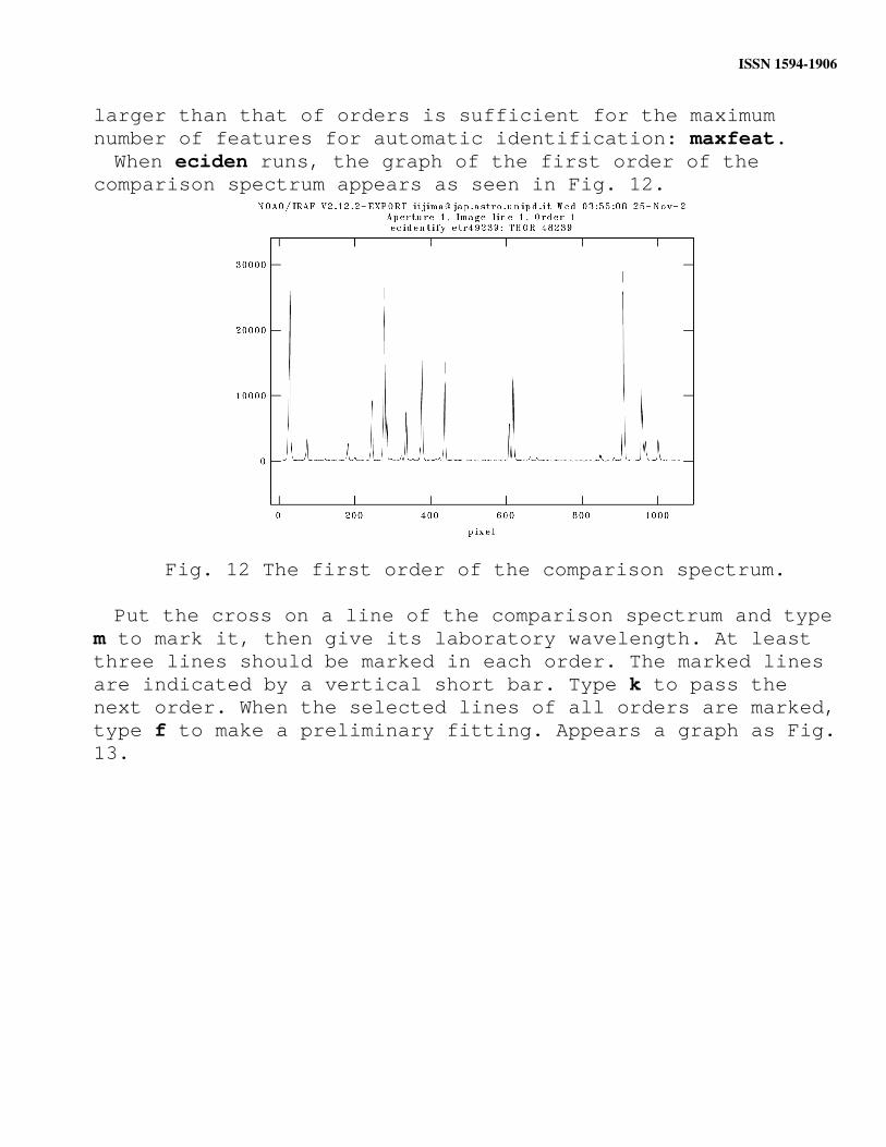
larger than that of orders is sufficient for the maximum number of features for automatic identification: maxfeat.When eciden runs, the graph of the first order of the

comparison spectrum appears as seen in Fig. 12.

Fig. 12 The first order of the comparison spectrum.

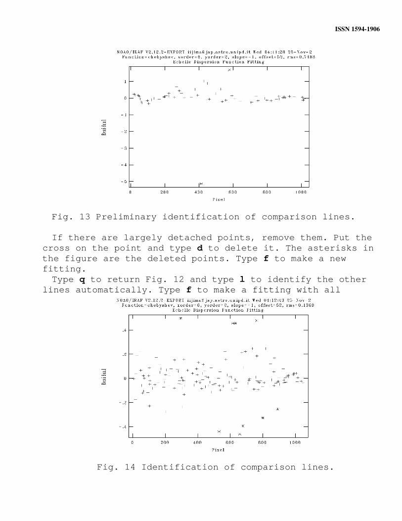
Put the cross on a line of the comparison spectrum and type m to mark it, then give its laboratory wavelength. At least three lines should be marked in each order. The marked lines are indicated by a vertical short bar. Type k to pass the next order. When the selected lines of all orders are marked, type f to make a preliminary fitting. Appears a graph as Fig. 13.

ISSN 1594­1906

Fig. 13 Preliminary identification of comparison lines.

If there are largely detached points, remove them. Put the cross on the point and type d to delete it. The asterisks in the figure are the deleted points. Type f to make a new fitting.Type q to return Fig. 12 and type l to identify the other

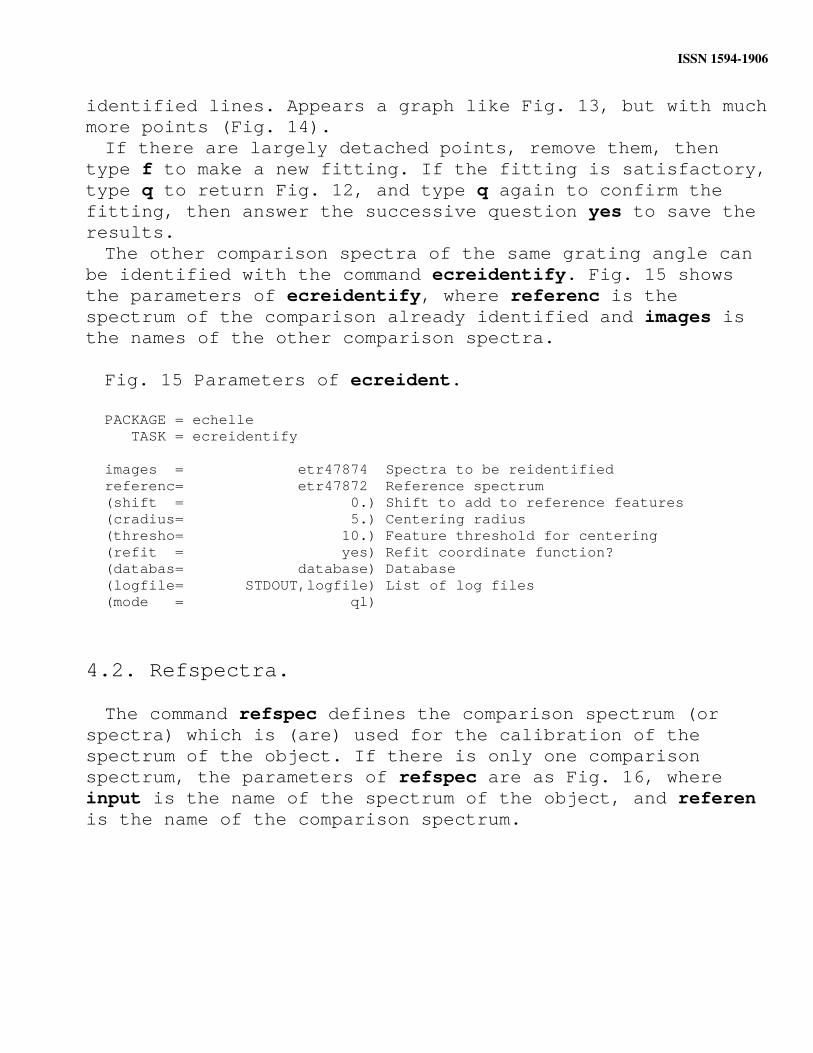
lines automatically. Type f to make a fitting with all

Fig. 14 Identification of comparison lines.

ISSN 1594­1906

identified lines. Appears a graph like Fig. 13, but with much more points (Fig. 14). If there are largely detached points, remove them, then

type f to make a new fitting. If the fitting is satisfactory, type q to return Fig. 12, and type q again to confirm the fitting, then answer the successive question yes to save the results.The other comparison spectra of the same grating angle can

be identified with the command ecreidentify. Fig. 15 shows the parameters of ecreidentify, where referenc is the spectrum of the comparison already identified and images is the names of the other comparison spectra.

Fig. 15 Parameters of ecreident.

PACKAGE = echelle TASK = ecreidentify

images = etr47874 Spectra to be reidentifiedreferenc= etr47872 Reference spectrum(shift = 0.) Shift to add to reference features(cradius= 5.) Centering radius(thresho= 10.) Feature threshold for centering(refit = yes) Refit coordinate function?(databas= database) Database(logfile= STDOUT,logfile) List of log files(mode = ql)

4.2. Refspectra.

The command refspec defines the comparison spectrum (or spectra) which is (are) used for the calibration of the spectrum of the object. If there is only one comparison spectrum, the parameters of refspec are as Fig. 16, where input is the name of the spectrum of the object, and referen is the name of the comparison spectrum.

ISSN 1594­1906

Fig. 16 Parameters of refspectra for one comparison spectrum.

PACKAGE = echelle TASK = refspectra

input = etr47873 List of input spectra(referen= etr47868) List of reference spectra(apertur= ) Input aperture selection list(refaps = ) Reference aperture selection list(ignorea= yes) Ignore input and reference apertures?(select = nearest) Selection method for reference spectra(sort = ) Sort key(group = ) Group key(time = no) Is sort key a time?(timewra= 17.) Time wrap point for time sorting(overrid= no) Override previous assignments?(confirm= yes) Confirm reference spectrum assignments?(assign = yes) Assign the reference spectra to the input spectra(logfile= STDOUT,logfile) List of logfiles(verbose= no) Verbose log output?answer = yes Accept assignment?(mode = ql)

On the other hand, if there are two comparison spectra obtained before and after the exposure of the object, the parameters are as in Fig. 17. When the exposure time is longer than one hour, or the

position of the object in the sky is low, say for airmass higher than 2.0, it is better to obtain two comparisons.

Fig. 17 Parameters of refspectra for two comparison spectra.

PACKAGE = echelle TASK = refspectra

input = etr47873 List of input spectra(referen= etr47868,etr47875) List of reference spectra(apertur= ) Input aperture selection list(refaps = ) Reference aperture selection list(ignorea= yes) Ignore input and reference apertures?(select = interp) Selection method for reference spectra(sort = jd) Sort key(group = ) Group key(time = no) Is sort key a time?

ISSN 1594­1906

(timewra= 17.) Time wrap point for time sorting(overrid= no) Override previous assignments?(confirm= yes) Confirm reference spectrum assignments?(assign = yes) Assign the reference spectra to the input spectra(logfile= STDOUT,logfile) List of logfiles(verbose= no) Verbose log output?answer = yes Accept assignment?(mode = ql)

Run refspec and answer yes the questions.

4.3. Wavelength calibrations.

Once the refspec process is completed the wavelength calibrations are made by using the command dispcor. Fig. 18 shows the parameters of dispcor.

Fig. 18 Parameters of dispcor.

PACKAGE = echelle TASK = dispcor

input = etr47873 List of input spectraoutput = etr47873.wl List of output spectra(lineari= yes) Linearize (interpolate) spectra?(databas= database) Dispersion solution database(table = ) Wavelength table for apertures(w1 = INDEF) Starting wavelength(w2 = INDEF) Ending wavelength(dw = 0.1) Wavelength interval per pixel(nw = INDEF) Number of output pixels(log = no) Logarithmic wavelength scale?(flux = yes) Conserve flux?(samedis= no) Same dispersion in all apertures?(global = no) Apply global defaults?(ignorea= no) Ignore apertures?(confirm= no) Confirm dispersion coordinates?(listonl= no) List the dispersion coordinates only?(verbose= yes) Print linear dispersion assignments?(logfile= ) Log file(mode = ql)

The input is the file of the one-dimensional spectrum of the object, and the output is the file in which the calib-rated spectrum will be saved. The author gives 0.1 for dw.

ISSN 1594­1906

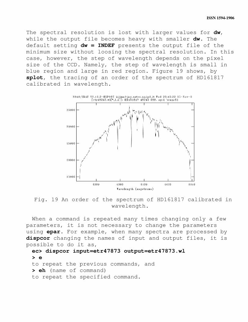
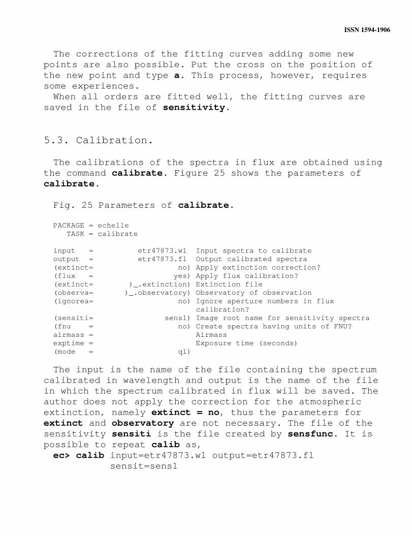
The spectral resolution is lost with larger values for dw, while the output file becomes heavy with smaller dw. The default setting dw = INDEF presents the output file of the minimum size without loosing the spectral resolution. In this case, however, the step of wavelength depends on the pixel size of the CCD. Namely, the step of wavelength is small in blue region and large in red region. Figure 19 shows, by splot, the tracing of an order of the spectrum of HD161817 calibrated in wavelength.

Fig. 19 An order of the spectrum of HD161817 calibrated in wavelength.

When a command is repeated many times changing only a few parameters, it is not necessary to change the parameters using epar. For example, when many spectra are processed by dispcor changing the names of input and output files, it is possible to do it as,ec> dispcor input=etr47873 output=etr47873.wl> eto repeat the previous commands, and> eh (name of command)to repeat the specified command.

ISSN 1594­1906

5. Flux calibration.

5.1. Standard.

The correction of the sensitivity of the spectrograph is made using the spectra of standard stars obtained in the same nights. The commands standard, sensfunct, and calibrate are used. Figure 20 shows the parameters of standard.

Fig. 20 Parameters of standard.

PACKAGE = echelle TASK = standard

input = etr47865.wl Input image file root nameoutput = std1 Output flux file (used by SENSFUNC)(samesta= yes) Same star in all apertures?(beam_sw= no) Beam switch spectra?(apertur= ) Aperture selection list(bandwid= 5.) Bandpass widths(bandsep= 5.) Bandpass separation(fnuzero= 3.6800000000000E-20) Absolute flux zero point(extinct= )_.extinction) Extinction file(caldir = onedstds$irscal/) Directory containing calibration data(observa= ekar) Observatory for data(interac= yes) Graphic interaction to define new band passes(graphic= stdgraph) Graphics output device(cursor = ) Graphics cursor inputstar_nam= hd161817 Star name in calibration listairmass = Airmassexptime = Exposure time (seconds)mag = Magnitude of starmagband = Magnitude typeteff = Effective temperature or spectral typeanswer = no (no|yes|NO|YES|NO!|YES!)(mode = ql)

The input is the name of the spectrum of the standard star calibrated in wavelength, and output is a name of file in which the properties of the standard star will be stored. Prior to the beginning of this process, it is necessary to remove standard files produced in the earlier works, which is done out of IRAF, e.g. $rm std* Give the name of the standard star in star_nam. In this

example the standard star is HD161817 and its data are

ISSN 1594­1906

contained in the directory onedstds$irscal/. The data of our observatory is given as ekar in IRAF. The band pass width bandwid and band pass separation bandsep are free parameters. The author uses 5.0 for both.Run standard and answer no the questions Edit bandpasses?

5.2. Sensitive function.

Figure 21 shows the parameters of sensfunc.

Fig. 21 Parameters of sensfunc.

PACKAGE = echelle TASK = sensfunc

standard= std1 Input standard star data file (from STANDARD)sensitiv= sens1 Output root sensitivity function image name(apertur= ) Aperture selection list(ignorea= no) Ignore apertures and make one sensitivity function(logfile= logfile) Output log for statistics information(extinct= )_.extinction) Extinction file(newexti= extinct.dat) Output revised extinction file(observa= )_.observatory) Observatory of data(functio= spline3) Fitting function(order = 2) Order of fit(interac= yes) Determine sensitivity function interactively?(graphs = sr) Graphs per frame(marks = plus cross box) Data mark types (marks deleted added)(colors = 2 1 3 4) Colors (lines marks deleted added)(cursor = ) Graphics cursor input(device = stdgraph) Graphics output deviceanswer = yes (no|yes|NO|YES)(mode = ql)

The input (standard) is the name of the file of the standard star created by the command standard and the output (sensitiv) is a name of file in which the fitting curves of the sensitivity will be saved. Again it is necessary to delete old sensitive files prior to this process, which is done in IRAF as: ec> imdel sens*.imh The author uses the function spline3 with an order 2.

ISSN 1594­1906

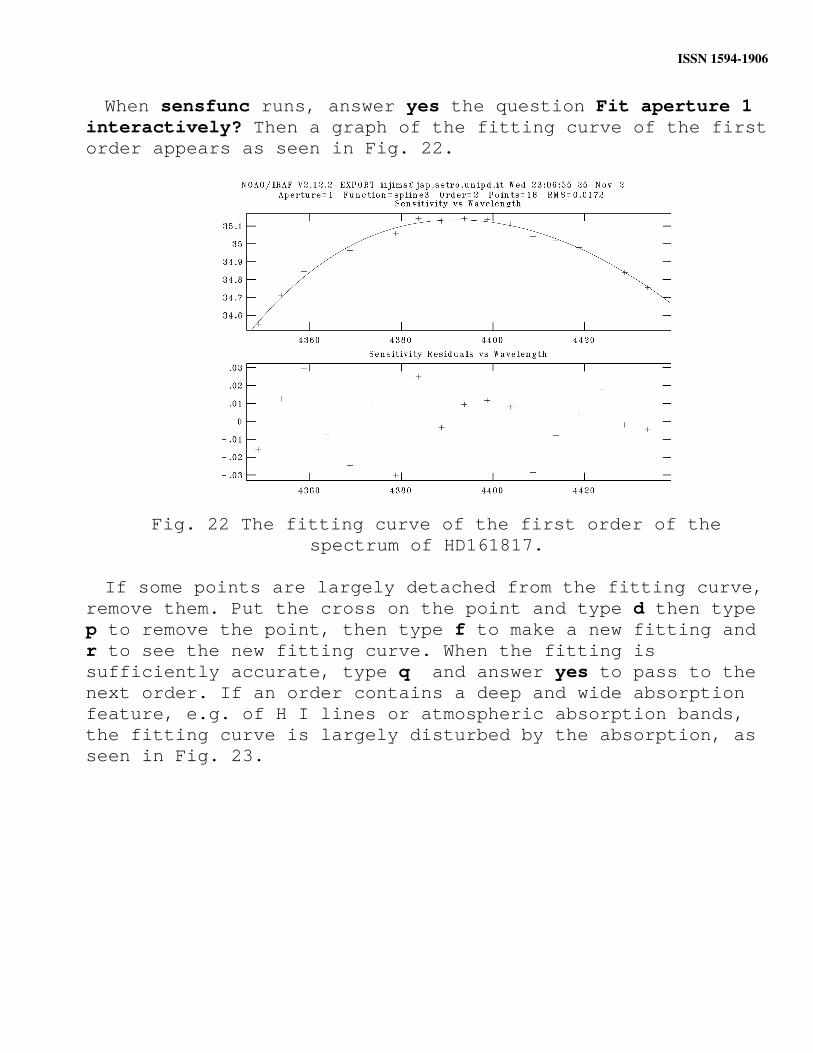
When sensfunc runs, answer yes the question Fit aperture 1 interactively? Then a graph of the fitting curve of the first order appears as seen in Fig. 22.

Fig. 22 The fitting curve of the first order of the spectrum of HD161817.

If some points are largely detached from the fitting curve, remove them. Put the cross on the point and type d then type p to remove the point, then type f to make a new fitting and r to see the new fitting curve. When the fitting is sufficiently accurate, type q and answer yes to pass to the next order. If an order contains a deep and wide absorption feature, e.g. of H I lines or atmospheric absorption bands, the fitting curve is largely disturbed by the absorption, as seen in Fig. 23.

ISSN 1594­1906

Fig. 23 A fitting curve disturbed by an absorption feature.

In such a case, all points related to the absorption feature have to be removed. Figure 24 shows a new fitting curve after the removal the points in the absorption.

Fig. 24 The fitting curve after the correction.

ISSN 1594­1906

The corrections of the fitting curves adding some new points are also possible. Put the cross on the position of the new point and type a. This process, however, requires some experiences.When all orders are fitted well, the fitting curves are

saved in the file of sensitivity.

5.3. Calibration.

The calibrations of the spectra in flux are obtained using the command calibrate. Figure 25 shows the parameters of calibrate.

Fig. 25 Parameters of calibrate.

PACKAGE = echelle TASK = calibrate

input = etr47873.wl Input spectra to calibrateoutput = etr47873.fl Output calibrated spectra(extinct= no) Apply extinction correction?(flux = yes) Apply flux calibration?(extinct= )_.extinction) Extinction file(observa= )_.observatory) Observatory of observation(ignorea= no) Ignore aperture numbers in flux calibration?(sensiti= sens1) Image root name for sensitivity spectra(fnu = no) Create spectra having units of FNU?airmass = Airmassexptime = Exposure time (seconds)(mode = ql)

The input is the name of the file containing the spectrum calibrated in wavelength and output is the name of the file in which the spectrum calibrated in flux will be saved. The author does not apply the correction for the atmospheric extinction, namely extinct = no, thus the parameters for extinct and observatory are not necessary. The file of the sensitivity sensiti is the file created by sensfunc. It is possible to repeat calib as,ec> calib input=etr47873.wl output=etr47873.fl sensit=sens1

ISSN 1594­1906

The results are seen by splot. Figure 26 shows the tracing of the order shown in Fig. 19 calibrated in flux.

Fig. 26 Tracing of an order of the spectrum of HD 161817 calibrated in flux.

5.4. Combining of orders.

The tracings of the orders calibrated in flux can be combined to one linear spectrum using the command scombine.Figure 27 shows the parameters of scombine.

Fig. 27 Parameters of scombine.

PACKAGE = echelle TASK = scombine

input = etr43527.fl List of input spectraoutput = etr43527.cm List of output spectra(noutput= ) List of output number combined spectra(logfile= STDOUT) Log file

(apertur= ) Apertures to combine(group = images) Grouping option(combine= average) Type of combine operation(reject = none) Type of rejection

ISSN 1594­1906

(first = no) Use first spectrum for dispersion?(w1 = INDEF) Starting wavelength of output spectra(w2 = INDEF) Ending wavelength of output spectra(dw = INDEF) Wavelength increment of output spectra(nw = INDEF) Length of output spectra(log = no) Logarithmic increments?

(scale = none) Image scaling(zero = none) Image zero point offset(weight = none) Image weights(sample = ) Wavelength sample regions for statistics

(lthresh= INDEF) Lower threshold(hthresh= INDEF) Upper threshold(nlow = 1) minmax: Number of low pixels to reject(nhigh = 1) minmax: Number of high pixels to reject(nkeep = 1) Minimum to keep (pos) or maximum to reject (neg)(mclip = yes) Use median in sigma clipping algorithms?(lsigma = 3.) Lower sigma clipping factor(hsigma = 3.) Upper sigma clipping factor(rdnoise= 0.) ccdclip: CCD readout noise (electrons)(gain = 1.) ccdclip: CCD gain (electrons/DN)(snoise = 0.) ccdclip: Sensitivity noise (fraction)(sigscal= 0.1) Tolerance for sigma clipping scaling corrections(pclip = -0.5) pclip: Percentile clipping parameter(grow = 0) Radius (pixels) for 1D neighbor rejection(blank = 0.) Value if there are no pixels(mode = ql)

The input is the name of the file of the spectrum calibrated in flux, and output is the name of file in which the combined spectrum will be saved. The parameter group is images and combine is average, respectively. The other parameters are default values. Figure 28 shows the combined spectrum.

ISSN 1594­1906

Fig. 28 Combined spectrum of HD161817.

It seems that the calibrations are obtained in a satisfactory manner. If the continuum appears as largely waving, there should have been some failures in the calibrations. In such a case, the corrections of the sensitivity of the spectrograph have to be made using the frame of flat field. Therefore, it is better to take some frames of the flat field in the night even if they are not used in our calibrations.Unfortunately, because of some technical problems, we have

to use a rather small CCD chip at the present time. This is the reason why there are gaps between the orders in the region redder than 4800Å.

The author is grateful to Prof. F. Strafella for the care-ful reading of the manuscript and the useful suggestions.If someone finds errors or knows better methods, please

contact with the author. (takashi.iijima@oapd.inaf.it)

10 February 2010

ISSN 1594­1906

Appendix

Introduction for IRAF2 beginners

Takashi IIJIMA

Astronomical Observatory of Padova, Asiago Station

2 IRAF is distributed by NOAO for Research in Astronomy, Inc. under cooperative agreement with the National Science Foundation.

ISSN 1594­1906

1. The first page of IRAF.

IRAF (Image Reduction and Analysis Facility) is a software developed by NOAO (National Optical Astronomy Observato-ries), for reductions of astronomical data. At first you have to make your login.cl file in your home

directory. Probably it is better to ask the operator of the computer. When you open IRAF, you will see the first page of IRAF as Figure 1.

Fig. 1 The first page of IRAF.

NOAO PC-IRAF Revision 2.12.2-EXPORT Sun Jan 25 16:09:03 MST 2004 This is the EXPORT version of PC-IRAF V2.12 supporting most PC systems.

Welcome to IRAF. To list the available commands, type ? or ??. To get detailed information about a command, type `help command'. To run a command or load a package, type its name. Type `bye' to exit a package, or `logout' to get out of the CL. Type `news' to find out what is new in the version of the system you are using. The following commands or packages are currently defined:

ace. dbms. graspo. mxtools. softools. vol. adccdrom. dimsum. guiapps. nlocal. spectime. xccdred. arcon. etools. ice. nmisc. spptools. xdimsum. ared. finder. ifocas. noao. sqiid. xdwred. aspec. fitsutil. images. nso. steward. xray. ccdacq. ftools. language. obsolete. stsdas. color. gemini. lists. plot. system. ctio. gmisc. mscred. proto. tables. dataio. grasp. mtools. rgo. utilities.cl>

The words without dot, which are not presented here, are names of commands, and the words with dot are names of directories where other commands and directories are contained. The branches of directories spread far and wide. For example, the commands for reductions of echelle spectra are found in the directory echelle and the path to there is:cl> noao > imred > echelle

The commands for reductions of grating spectra are:cl> noao > twodspec > apextract for extractions of one-dimensional spectra andcl> noao > onedspec

ISSN 1594­1906

for further analyses. The path below is also possible.cl> noao > twodspec > apextract > onedspec

The commands for analyses of nebular emission lines are found in the directory nebular and the path is:cl> stsdas > analysis > nebular

As written in Fig. 1, the command >bye allows you to exit the current directory and return to the previous one. However, it is not necessary to go back the previous directory to use the commands contained there. For example, if you are now in the directory echelle, you can use also all commands in cl, noao, and imred, and you can go to any directory presented there. The names of commands and directories can be abbreviated unless ambiguity occurs with other names.

2. How to display the images.

The commands to display images are found in the directory tv.cl> images > tv

The window SAOimage ds9 to display the images has to be opened out of IRAF separately. You can see an image with the command display as:tv> display (name of an image file) 1

It is necessary to give the number 1, even if there is only one device to display images.

All commands of IRAF contain numerous hidden parameters which determine the operations of the commands. You can change the operations of the commands into your own manner changing the parameters. For example, the command display in the default setting determines automatically the minimum and maximum levels of the image displayed in the window ds9. It is, however, possible to display the image with different dynamic ranges as follows. Figure 2 shows the window of the

ISSN 1594­1906

hidden parameters of display which opens with the command:tv> epar display

Fig. 2 Hidden parameters of the command display.

PACKAGE = tv TASK = display

image = image to be displayedframe = 1 frame to be written into(bpmask = BPM) bad pixel mask(bpdispl= none) bad pixel display (none|overlay|

interpolate)(bpcolor= red) bad pixel colors(overlay= ) overlay mask(ocolors= green) overlay colors(erase = yes) erase frame(border_= no) erase unfilled area of window(select_= yes) display frame being loaded(repeat = no) repeat previous display parameters(fill = yes) scale image to fit display window(zscale = yes) display range of greylevels near median(contras= 0.25) contrast adjustment for zscale algorithm(zrange = yes) display full image intensity range(zmask = ) sample mask(nsample= 1000) maximum number of sample pixels to use(xcenter= 0.5) display window horizontal center(ycenter= 0.5) display window vertical center(xsize = 1.) display window horizontal size(ysize = 1.) display window vertical size(xmag = 1.) display window horizontal magnification(ymag = 1.) display window vertical magnification(order = 0) spatial interpolator order (0=replicate, 1=linea(z1 = ) minimum greylevel to be displayed(z2 = ) maximum greylevel to be displayed(ztrans = linear) greylevel transformation (linear|log|none| user)(lutfile= ) file containing user defined look up table(mode = ql)

Change the parameters into zsacle = no and zrange = no, then CTR-d to save the changes and close the window. (CTR-c to close the window loosing the changes.) You can see the image with your own range, for example, as:tv> display (name of image) 1 z1=1000 z2=5000

Now the dynamic range of the image in the display is 1000-

ISSN 1594­1906

5000. In this case, the changes of the parameters are kept until the next changes, namely you have to give z1 and z2 every time. On the other hand, you can see the image with the same dynamic range as:tv> display (name) 1 zscale=no zrange=no z1=1000 z2=5000

In this case, the changes of the parameters are valid only in this operation.The command unlearn cleans up all changes of the parameters

of the commands and resets the default parameter values.> unlearn (name of command)

3. Structure of IRAF image files.

The formats of image files used in IRAF are of FITS (**.fits) and IRAF (**.imh). Image files created by the commands of IRAF usually have the format IRAF (**.imh). An image file of IRAF format consists of a header file

(**.imh) and a pixel file (**.pix). You can define the folder to keep the pixel files in your login.cl file. The header and pixel files are dealt with as if they were

a unique file in IRAF. It is sufficient to give the names of the header files for all IRAF commands. On the other hand, if you want to keep the IRAF image files in a certain device, or if you want to send them by ftp or by e-mail, the format has to be converted to the FITS format by the command wfits in the directory dataio.da> wfits (name of IRAF file) (name of FITS file)

You can not operate on IRAF image files by the commands of Linux. For example, you can not correctly remove, copy, or rename the IRAF image files with Linux commands: rm, cp, or mv. These operations have to be applied contemporaneously to the header and pixel files, which are made by the commands in the directory images of IRAF, as:im> imdel (name of files)im> imcopy (name of files) (name of files or directory)im> imrename (name of files) (name of files or directory)

ISSN 1594­1906

The other frequently used commands for image files are:im> imhead ht*Lists up all image files with names started by ht.

im> imhead (name of a file) l+Shows the full header of the image file.

im> imstatis (name of a file)Shows the statistics of the image file.im> imarith (name) (operator) (name) (name of output)Applies arithmetic operations +,-,*,/ etc. to image files.

4. Splot and others.

Most of the astronomical quantities: wavelength, fwhm, equivalent width, flux, etc., can be measured using the tools in the command splot. It is also possible to do the decompositions of emission and absorption lines by splot. See the very long help of splot in detail. The command splot is found in various directories, e.g., in echelle and onedspec.

The command >e allows you to repeat the previous commands, and > eh (name of command)to repeat the specified command.

> help Lists up the commands in the current directory and shows

their short explanations.

> help (name of command)Shows the detailed explanation of the command.

>logout to end IRAF.