Pad6 Approximants - Type I and Type II - and Their Application
20
Pad6 Approximants - Type I and Type II - and Their Application Clyde Chlouber McDonnell Douglas 16055 Space Center Blvd. Houston, Texas 77062 and Guowen Li and Mark A. Samuel Department of Physics Oklahoma State University Stillwater, Oklahoma 74078 1 ROtn t-._ ..... _- ! t'--.·c.-_- .. , .. " ). February, 199r-- .. OSU Research Note 265 I r""' ........
Transcript of Pad6 Approximants - Type I and Type II - and Their Application

Pad6 Approximants - Type I and Type II - and Their Application
Clyde Chlouber McDonnell Douglas
16055 Space Center Blvd Houston Texas 77062
and
Guowen Li and Mark A Samuel Department of Physics
Oklahoma State University Stillwater Oklahoma 74078
1 ROtn t-_ _shy
~
t--middotc-_- )
~ February 199r--middotmiddot-centgtmiddot~~middot-OSU Research Note 265
~-~-~-
Ir ~
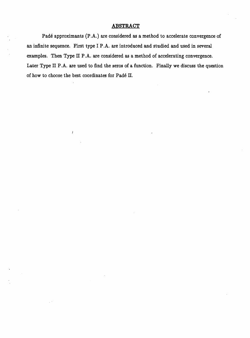
ABSTRACT
Pade approximants (P A) are considered as a method to accelerate convergence of
an infinite sequence First type I P A are introduced and studied and used in several
examples Then Type II P A are considered as a method of accelerating convergence
Later Type II P A are used to find the zeros of a function Finally we discuss the question
of how to choose the best coordinates for Pade II
2
I TYPE I P ADt APPROXIMANTS
Definition Let f(z) be an analytic function defined by its Taylor series
CD
nf(z) = L anz
n=Q
The Pade approximate to the function f(z) is defined as
~nml(z) = P n (z) = f(z) + O(zn+m+1) (1)Qm(z)
P n(z) and Qm(z) are polynomials of degree n and m egPn(z) = bl + b2z + + bNzn
P n (z)The meaning of is that we can wnte
Qm(z)
P n (z) n+m+l + d zn+m+z +( ) (2)f z = Qm(z) + dn+ m+ l z n+m+z
~~----------------~--------------~IO(zn+m+l )
where the ds and also the coefficients of z in the Pade approximate are functions of the
coefficients in the Taylor series expansion
For n = m ~nn](z) is called a diagonal PA
Rationale for making this kind of approximation
1) A rational fraction can approximate a function near singularities where the
approximation by polynomials breaks down
2) Will find that we can often get good approximations to the function value from a
Pade approximant constructed from the 1st several Taylor series coefficients
3 shy
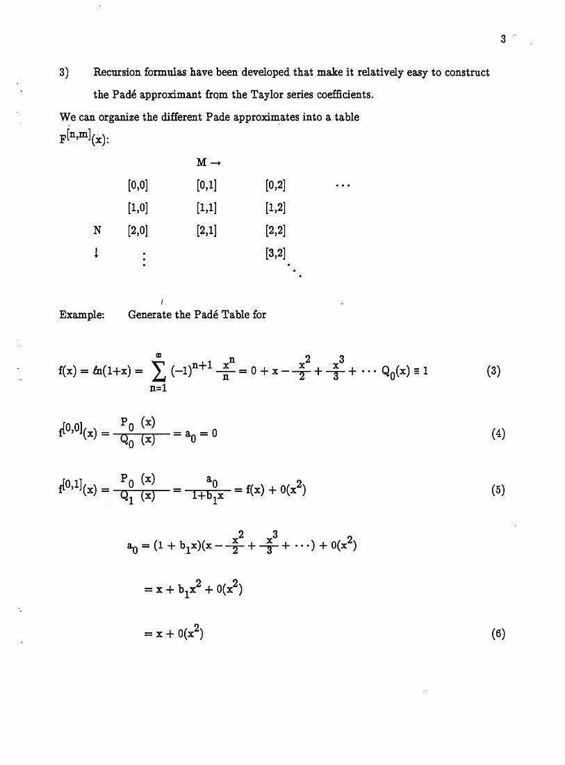
3) Recursion formulas have been developed that make it relatively easy to construct
the Pade approximant frQm the Taylor series coefficients
We can organize the different Pade approxiIDates into a table
F[nm](x)
M--+
[00] [01] [02]
[10] [11] [12]
N [20] [21] [22]
1 [32]
J
Example Generate the Pade Table for
OJ n 2 3 f(x) = io(1+x) = L (_l)n+1 = 0 + x -++++ QO(x) 1 (3)
n=l
~ool(x) = Po (x) (4)(x)QO
~oll(x) = Po (x) (5)Q1 (x)
(6)
---------------------- --_
4 shy
We cant find a value for aOthat is independent of x so lets look at the lower half of
the Pade table
pOl(x) = PI (x) (7)QO (xJ
(8)
~111(x) = PI (x)Q1 (x) (9)
(10)
~11](X) =---xl-- (11) 1+ -rx
~11](1) = 23 (12)
Note tn 2 = 69314 (13)
(14)
5
2 1 2 b1 1 3 4 aO+ a1x + ~x = x + (b1 ---r)x + (-2+ -)x + O(x ) (15)
aO = 0
1a1 =
b1 =-2
a2 = 16
2x + 1 x~21](x) =--~-2~- (16)
1 + -X
~21](1) = 7 (17)
1 2 ~221(x) = x + -r x
1 + x+ +x2 (20)
~22](1) = 6923 (21)
1 1 1d 1 - --r +-- -r = 58 (22)
Discussion of the convergence properties of the Pade Type 1 approximants and recursive
schemes to calculate the coefficients are given by J Zinn-Justin and Baker
6
II Pade Tyne II Approximants (Introduction)
Definition Let z1 z2 zp be p numbers for which the analytic function f(z) is
defined
The Pade Type II Approximent is defined to be
P~nm](z) =~ (23) ~
with ~nm](zi) =f(zi) for
i =12middot middot p and p =m + n + 1
As before P n (z) and Q (z) are polynomials of degree nand m m J _
Let us restrict our attention to the diagonal Pade approximants for which n =m =N
Then for each of the 2N + 1 coordinate zk we can write
N iL a Zk1
~NN](zk) = i=o Sk = f(zk) (24)N shy
L bj z~ j=o
For many problems of practical interest we may know the values of the function (S1
S2N+ 1) corresponding to a range of coordinates
zl gt z2 gt gt z2N+l gt 0 for example
We may not know the value of the function at z = 0 however We can obtain an
approximation to the value f(O) by constructing the Pade Type II approximant using the
known values of the functi9n f(~)
(25)
7 shy
Solve for coefficient aO
N N N
Sk lgtj4= Sk(l + Lbj zt) = Lai z~ j=O j=l i=O
(26)
We have 2N + 1 equations for the unknown ai and bi which we can write as a matrix
equation
2 NzN1 zl zl -Slzl -S 1 z 1 1 N
1 z2 -S 2 z 2
N N1 z2N+l z2N+l -S2N+l Z2N+lmiddotmiddotmiddot -S2N+l z2N+l
a O
a middot l middot middot aN
b middot l middot bN
-
SI
S2
(27)
S2N+l
8
Using Cramers Rule solve for aO
(28)
N1 -S2N+l z 2N+l
9
m Example for Pade Type II
Suppose that we want to find the sum of the series
(29)
Regarding S as the limit of a sequence of functions (Partial Sums)
00 - 1
Sk = ) --r is the kth partial sum (30) ~-J n n=l
So that for example the first 3 partial sums are
SI = 1
S2 =1 ++= 542
S3 =1 ++++= 4936 (31)2 3
Having 3 partial sums we just need 3 coordinates zl z2 z3 to construct the ~11] Pade
approximant
A valid choice for the coordinate associated with the kth partial sum of this particular
series is
(32)
Then for the [11] approximate
Jll] aO+a1z fl (z) = 1 +h z (33)
1
We demand that the PA be equal to the partial sums at zl =lz2 =+ za =+ (34)
(35)
10
aO+i11](+) = 1 +
1 1
1 1
1 13
1
54
4936
aO =
a1i3 _ 49 61 3 -36
1-1 aO
-58 54-a1
--49108 4936b1
i -1
12 -58
13 --49108
(36)
(37)
1 1 -1
1 12 -58
1 13 --49108
1 1
0 -34
0 0
1 1 -1
0 -12 38
0 0 5108
This is to be compared with the lIexact answer
e(2) = 1f21Ji ~ 16449
Also note that the 3rd partial sum S3 = 13
-1
58
11 216
33- 20= 165 (38)
11
IV Using Pade II approximates to find the zero of a function
Let f(z) be the function for which we want to find the value of z that satisfies the equation
f(z) = 0 (40)
We start with 3 points zldeg z2 z3 for which we evaluate
f1 = f(zl)
f2 =f(z2)
f3 = f(z3) (41)
We then build the [11] Pade Type II approximate
i = 123 (42)
writing these 3 equations as a matrix equation
(43)
1
M= 1 (44)N
1
Solving for the coefficients aOand a1
12
f1 zl -f1z1
-f (45)~ z2 2z2
fa za -faza
aO =
IyenI 1 zl -f1z1
a1 = 1 Z2 -~z2 (46)
1 za -faza
I yen I The 1st approximation to the zero of fez) is given by the solution to the simpler equation
~ll](z) = 0 (47)
or
(48)
(49)
We can then set up an iterative scheme replacing the coordinates zl z2 and za by the zNEW
13
V Type IT Pade Approximants (continued)
We now discuss methods of extrapolating certain types of convergent sequences Sl
S2 SK to the limit
it S = k -+ 00 Sk
using Pade type II approximants An excellent review is given by J Zinn-Justin1
Definition Let z1 zp be p complex numbers f( z) a given analytic function
The [nm] Pade tyope II approximant is the rational fraction
~nml(z) = P n (z) (50)Qm(z)
with ~nml (zi) = f(~i) for i = 1 2 bull p and n + m + i = p Pn and Q arem polynomials of degree n and m respectively
J Zinn Justin1 gives the following convergence theorem analogous to a convergence
theorem for the usual Pade approximants proved by Nutall2
Theorem If fez) is a function of the Stie1tjes3 type and if the points zi are chosen
on a compact set of the real axis on the right of all singularities of the function then the
sequence of Pade approximations converges toward the function because the zero of the
denominators are on the cut of f(z)
In particular we consider the application of Pade type II approximants to the
00 k problem of summing an infinite series S = E U whose kth partial sum is Sk = E U
1 1 bull 1 11= 1=
The diagonal approximant is defined to be
aO + a1Z + + an Zn
[]S nn (z) = ------_____ (51)1 + b1Z + + b Zn n
with S[nn] (Zk) = Ski k = 1 2n + 1 We define the Pade approximant to the sum S to be
14
S[nn] (0) = a O
Consideration of a simple example shows that the rate of convergence of the
approximants to the sum S is sensitive to the choice of the ZKo For example consider e 00 1 r2 1 1 3 3
0 0(2) = E --r = 6 Take as co--ordinates Zk = ---p- Pe- -r 1- 2 The n=l n k
results shown in Table I for S[221(0) I 1 show that the simple choice45 ~ = Zk=y-shy
+gives the best agreement with the exact result
e(2) = 164493406684822643637 bullbull (52)0
In fact if we evaluate ~551(0) I 1 we obtain ll-place agreement with the exact Zk= -c
result
TABLE I
PADE TYPE II APPROXIMANTS TO e(2) FOR DIFFERENT CHOICES
OF CO-ORDINATES
P
12 34 1
32 2
164668 165594
164489
161145
158065
In order to arrive at a rule for systematically choosing the Zk let us consider the
expression for aO
15
n SI zl zl -SIzl -SIZ~ S2 z2
n nS2n+l z2n+l middotz2n+l -S2n+l Z2n+l (53)aO =
1 zl -Slz~ 1
1 Z2n+l
We notice that aO = S if the co-ordinates zk are chosen as
(54)
We then have S[nn](o) = S and the PA is exact We see that the set zk is on a
compact set of the real axis with the origin as an accumulation point For example if the
given series is convergent and monotonically increasing such that 0 lt Uk+ l lt Uk then
we have 0 lt zk+l and we can choose the zks on [01]
We can now understand why zk = +is an appropriate choice of co-ordinates for
summing e(2) Consider the kth partial sum Sk The remainder is
00 1 - E --r
m=k+l m
We can easily show that kr lt Rk+ l lt + The point is that for large k Rk+ 1 N + Hence for large k the co-ordinates are approximately
16
kraquo 1 (55)
Now S[nn](O) is invariant under the transformation zk -+ C zk where C is an
arbitrary normalizing constant consequently we may simply choose
kraquol (56)
An example for which we may determine the co-ordinates exactly is the geometric series
k We have Sk = i=~ S = l~r and zk = rk In general we can not find the Itcorrectll coshy
ordinates zk since we would need to know the sum of the series however as a method of J _
approximating the sum of a series of positive terms we can try to determine the
asymptotic form of the remainder and then use the asymptotic approximation for the zk
for all k
We now consider an example that is particularly relevant to the evaluation of an
integral whose integrand has a singularity in its zeroth or first derivative at one of the
endpoints of the integration interval
Suppose that a positive series S is asymptotically geometric By this we mean
it Uk+m mk-iOO 0 = r where 0 lt r lt 1 and mel 2 bullbullbull Then the asymptotic form of the
k S-Sk
co-ordinates zk S for the Pade type n approximant is
(57)
For consider
(58)
17
but since U k +m --+ rm as k --+ 00 we haveUk
(59)
Noting the invariance of S[nn] (0) under zk --+ C zk we have the result
As an example of the application of this result to the evaluation of an integral we
consider the integral representation of e(2) 1
S = e(2) = - r dt In(l-t) (60)tJO We consider e(2) as a limit of a sequence of partial sums
(61)
where 0 lt ck lt 1
Uk+mDefinmg Uk = Sk - Sk-l we form 0k Upon letting ek+m = rmek with 0 lt r lt I
we find that
m _l-r ek In(l-t) dtm-l t
Uk + m _ l-r ck mkLLoo it =r (62)Ok ck ---t 0 m
_l-r ek In(l-t) dtm-l tl-r ck
Consequently the asymptotic form of the Pade type II co-ordinates is
k--+oo UZk I k
On the other hand we can study the analytic structure of the sequence of functions
Sk(k = 12 ) numerically Let the interval [01] be divided into m = 12481632
subintervals This choice corresponds to setting r = 12 An eight point Gauss quadrature
18
is then applied to each subinterval and the results of all the subintervals are summed
Thus a sequence of approximant partial sums Sk shown in column 1 of Table II is obtained
The results shown in columns 2 or 3 of Table II clearly show the geometric character of the
convergence Using the co-ordinates Zk =UkU l we obtain for the P ade extrapolation
5[22](0)1 U = 1644934066848720 k
Zk =ushy1
This remarkable result agrees with e(2) to 13 decimal places (a 9 place improvement over
the last quadrature approximation S6) It should be remembered however that 504
function evaluations were required to obtain this number Also the convergence is not
nearly so rapid for sorite other functions eg e(3)
TABLEll
SEQUENCE OF QUADRATURE APPROXIMATIONS S K IS SHOWN ALONG
WITH DIFFERENCES Uk AND NORMALIZED CO-ORDINATES Zk ~
sk k Uk = Sk+l - Sk Zk = UkUi
1 1636221116771679 4344583280914582 I 10-3 1
2 1640565700052593 2181170094296302 I 10-3 5020435685693985
3 1642796870146890 1092839813718882 I 10-3 2515407696772230
4 1643839709960609 5469881472146554 J 10--4 1259011766715422
5 1644386698110782 2736367125502070 J 10--4 0629834197798145
6 1644660334820374
The geometric interval method is most useful when the integrand or its first
derivative is singular at one of the endpoints of the integration interval
19
REFERENCES
1 J Zinn-Justin Physics Reports 1 No3 1971 55-102
2 J Nutall J Math Anal 31 147-153 (1970)
3 Stieltjes functions have a cut on the real axis and satisfy Im[fz)] 1m z ~ 0 in the cut
plane See G A Baker J Adv Theor Phys 1 (1965) 1
4 J L Basdevant (1968) Pade Approximants Ecole Internationale de La Phsique
des Particules Elementaires Herceq Novi (Yougoslavie) Cent Rech Nuci
Stras bourg France
5 R Bulirsch and J Stoer Numer Math 2 413-427 (1964)
ABSTRACT
Pade approximants (P A) are considered as a method to accelerate convergence of
an infinite sequence First type I P A are introduced and studied and used in several
examples Then Type II P A are considered as a method of accelerating convergence
Later Type II P A are used to find the zeros of a function Finally we discuss the question
of how to choose the best coordinates for Pade II
2
I TYPE I P ADt APPROXIMANTS
Definition Let f(z) be an analytic function defined by its Taylor series
CD
nf(z) = L anz
n=Q
The Pade approximate to the function f(z) is defined as
~nml(z) = P n (z) = f(z) + O(zn+m+1) (1)Qm(z)
P n(z) and Qm(z) are polynomials of degree n and m egPn(z) = bl + b2z + + bNzn
P n (z)The meaning of is that we can wnte
Qm(z)
P n (z) n+m+l + d zn+m+z +( ) (2)f z = Qm(z) + dn+ m+ l z n+m+z
~~----------------~--------------~IO(zn+m+l )
where the ds and also the coefficients of z in the Pade approximate are functions of the
coefficients in the Taylor series expansion
For n = m ~nn](z) is called a diagonal PA
Rationale for making this kind of approximation
1) A rational fraction can approximate a function near singularities where the
approximation by polynomials breaks down
2) Will find that we can often get good approximations to the function value from a
Pade approximant constructed from the 1st several Taylor series coefficients
3 shy
3) Recursion formulas have been developed that make it relatively easy to construct
the Pade approximant frQm the Taylor series coefficients
We can organize the different Pade approxiIDates into a table
F[nm](x)
M--+
[00] [01] [02]
[10] [11] [12]
N [20] [21] [22]
1 [32]
J
Example Generate the Pade Table for
OJ n 2 3 f(x) = io(1+x) = L (_l)n+1 = 0 + x -++++ QO(x) 1 (3)
n=l
~ool(x) = Po (x) (4)(x)QO
~oll(x) = Po (x) (5)Q1 (x)
(6)
---------------------- --_
4 shy
We cant find a value for aOthat is independent of x so lets look at the lower half of
the Pade table
pOl(x) = PI (x) (7)QO (xJ
(8)
~111(x) = PI (x)Q1 (x) (9)
(10)
~11](X) =---xl-- (11) 1+ -rx
~11](1) = 23 (12)
Note tn 2 = 69314 (13)
(14)
5
2 1 2 b1 1 3 4 aO+ a1x + ~x = x + (b1 ---r)x + (-2+ -)x + O(x ) (15)
aO = 0
1a1 =
b1 =-2
a2 = 16
2x + 1 x~21](x) =--~-2~- (16)
1 + -X
~21](1) = 7 (17)
1 2 ~221(x) = x + -r x
1 + x+ +x2 (20)
~22](1) = 6923 (21)
1 1 1d 1 - --r +-- -r = 58 (22)
Discussion of the convergence properties of the Pade Type 1 approximants and recursive
schemes to calculate the coefficients are given by J Zinn-Justin and Baker
6
II Pade Tyne II Approximants (Introduction)
Definition Let z1 z2 zp be p numbers for which the analytic function f(z) is
defined
The Pade Type II Approximent is defined to be
P~nm](z) =~ (23) ~
with ~nm](zi) =f(zi) for
i =12middot middot p and p =m + n + 1
As before P n (z) and Q (z) are polynomials of degree nand m m J _
Let us restrict our attention to the diagonal Pade approximants for which n =m =N
Then for each of the 2N + 1 coordinate zk we can write
N iL a Zk1
~NN](zk) = i=o Sk = f(zk) (24)N shy
L bj z~ j=o
For many problems of practical interest we may know the values of the function (S1
S2N+ 1) corresponding to a range of coordinates
zl gt z2 gt gt z2N+l gt 0 for example
We may not know the value of the function at z = 0 however We can obtain an
approximation to the value f(O) by constructing the Pade Type II approximant using the
known values of the functi9n f(~)
(25)
7 shy
Solve for coefficient aO
N N N
Sk lgtj4= Sk(l + Lbj zt) = Lai z~ j=O j=l i=O
(26)
We have 2N + 1 equations for the unknown ai and bi which we can write as a matrix
equation
2 NzN1 zl zl -Slzl -S 1 z 1 1 N
1 z2 -S 2 z 2
N N1 z2N+l z2N+l -S2N+l Z2N+lmiddotmiddotmiddot -S2N+l z2N+l
a O
a middot l middot middot aN
b middot l middot bN
-
SI
S2
(27)
S2N+l
8
Using Cramers Rule solve for aO
(28)
N1 -S2N+l z 2N+l
9
m Example for Pade Type II
Suppose that we want to find the sum of the series
(29)
Regarding S as the limit of a sequence of functions (Partial Sums)
00 - 1
Sk = ) --r is the kth partial sum (30) ~-J n n=l
So that for example the first 3 partial sums are
SI = 1
S2 =1 ++= 542
S3 =1 ++++= 4936 (31)2 3
Having 3 partial sums we just need 3 coordinates zl z2 z3 to construct the ~11] Pade
approximant
A valid choice for the coordinate associated with the kth partial sum of this particular
series is
(32)
Then for the [11] approximate
Jll] aO+a1z fl (z) = 1 +h z (33)
1
We demand that the PA be equal to the partial sums at zl =lz2 =+ za =+ (34)
(35)
10
aO+i11](+) = 1 +
1 1
1 1
1 13
1
54
4936
aO =
a1i3 _ 49 61 3 -36
1-1 aO
-58 54-a1
--49108 4936b1
i -1
12 -58
13 --49108
(36)
(37)
1 1 -1
1 12 -58
1 13 --49108
1 1
0 -34
0 0
1 1 -1
0 -12 38
0 0 5108
This is to be compared with the lIexact answer
e(2) = 1f21Ji ~ 16449
Also note that the 3rd partial sum S3 = 13
-1
58
11 216
33- 20= 165 (38)
11
IV Using Pade II approximates to find the zero of a function
Let f(z) be the function for which we want to find the value of z that satisfies the equation
f(z) = 0 (40)
We start with 3 points zldeg z2 z3 for which we evaluate
f1 = f(zl)
f2 =f(z2)
f3 = f(z3) (41)
We then build the [11] Pade Type II approximate
i = 123 (42)
writing these 3 equations as a matrix equation
(43)
1
M= 1 (44)N
1
Solving for the coefficients aOand a1
12
f1 zl -f1z1
-f (45)~ z2 2z2
fa za -faza
aO =
IyenI 1 zl -f1z1
a1 = 1 Z2 -~z2 (46)
1 za -faza
I yen I The 1st approximation to the zero of fez) is given by the solution to the simpler equation
~ll](z) = 0 (47)
or
(48)
(49)
We can then set up an iterative scheme replacing the coordinates zl z2 and za by the zNEW
13
V Type IT Pade Approximants (continued)
We now discuss methods of extrapolating certain types of convergent sequences Sl
S2 SK to the limit
it S = k -+ 00 Sk
using Pade type II approximants An excellent review is given by J Zinn-Justin1
Definition Let z1 zp be p complex numbers f( z) a given analytic function
The [nm] Pade tyope II approximant is the rational fraction
~nml(z) = P n (z) (50)Qm(z)
with ~nml (zi) = f(~i) for i = 1 2 bull p and n + m + i = p Pn and Q arem polynomials of degree n and m respectively
J Zinn Justin1 gives the following convergence theorem analogous to a convergence
theorem for the usual Pade approximants proved by Nutall2
Theorem If fez) is a function of the Stie1tjes3 type and if the points zi are chosen
on a compact set of the real axis on the right of all singularities of the function then the
sequence of Pade approximations converges toward the function because the zero of the
denominators are on the cut of f(z)
In particular we consider the application of Pade type II approximants to the
00 k problem of summing an infinite series S = E U whose kth partial sum is Sk = E U
1 1 bull 1 11= 1=
The diagonal approximant is defined to be
aO + a1Z + + an Zn
[]S nn (z) = ------_____ (51)1 + b1Z + + b Zn n
with S[nn] (Zk) = Ski k = 1 2n + 1 We define the Pade approximant to the sum S to be
14
S[nn] (0) = a O
Consideration of a simple example shows that the rate of convergence of the
approximants to the sum S is sensitive to the choice of the ZKo For example consider e 00 1 r2 1 1 3 3
0 0(2) = E --r = 6 Take as co--ordinates Zk = ---p- Pe- -r 1- 2 The n=l n k
results shown in Table I for S[221(0) I 1 show that the simple choice45 ~ = Zk=y-shy
+gives the best agreement with the exact result
e(2) = 164493406684822643637 bullbull (52)0
In fact if we evaluate ~551(0) I 1 we obtain ll-place agreement with the exact Zk= -c
result
TABLE I
PADE TYPE II APPROXIMANTS TO e(2) FOR DIFFERENT CHOICES
OF CO-ORDINATES
P
12 34 1
32 2
164668 165594
164489
161145
158065
In order to arrive at a rule for systematically choosing the Zk let us consider the
expression for aO
15
n SI zl zl -SIzl -SIZ~ S2 z2
n nS2n+l z2n+l middotz2n+l -S2n+l Z2n+l (53)aO =
1 zl -Slz~ 1
1 Z2n+l
We notice that aO = S if the co-ordinates zk are chosen as
(54)
We then have S[nn](o) = S and the PA is exact We see that the set zk is on a
compact set of the real axis with the origin as an accumulation point For example if the
given series is convergent and monotonically increasing such that 0 lt Uk+ l lt Uk then
we have 0 lt zk+l and we can choose the zks on [01]
We can now understand why zk = +is an appropriate choice of co-ordinates for
summing e(2) Consider the kth partial sum Sk The remainder is
00 1 - E --r
m=k+l m
We can easily show that kr lt Rk+ l lt + The point is that for large k Rk+ 1 N + Hence for large k the co-ordinates are approximately
16
kraquo 1 (55)
Now S[nn](O) is invariant under the transformation zk -+ C zk where C is an
arbitrary normalizing constant consequently we may simply choose
kraquol (56)
An example for which we may determine the co-ordinates exactly is the geometric series
k We have Sk = i=~ S = l~r and zk = rk In general we can not find the Itcorrectll coshy
ordinates zk since we would need to know the sum of the series however as a method of J _
approximating the sum of a series of positive terms we can try to determine the
asymptotic form of the remainder and then use the asymptotic approximation for the zk
for all k
We now consider an example that is particularly relevant to the evaluation of an
integral whose integrand has a singularity in its zeroth or first derivative at one of the
endpoints of the integration interval
Suppose that a positive series S is asymptotically geometric By this we mean
it Uk+m mk-iOO 0 = r where 0 lt r lt 1 and mel 2 bullbullbull Then the asymptotic form of the
k S-Sk
co-ordinates zk S for the Pade type n approximant is
(57)
For consider
(58)
17
but since U k +m --+ rm as k --+ 00 we haveUk
(59)
Noting the invariance of S[nn] (0) under zk --+ C zk we have the result
As an example of the application of this result to the evaluation of an integral we
consider the integral representation of e(2) 1
S = e(2) = - r dt In(l-t) (60)tJO We consider e(2) as a limit of a sequence of partial sums
(61)
where 0 lt ck lt 1
Uk+mDefinmg Uk = Sk - Sk-l we form 0k Upon letting ek+m = rmek with 0 lt r lt I
we find that
m _l-r ek In(l-t) dtm-l t
Uk + m _ l-r ck mkLLoo it =r (62)Ok ck ---t 0 m
_l-r ek In(l-t) dtm-l tl-r ck
Consequently the asymptotic form of the Pade type II co-ordinates is
k--+oo UZk I k
On the other hand we can study the analytic structure of the sequence of functions
Sk(k = 12 ) numerically Let the interval [01] be divided into m = 12481632
subintervals This choice corresponds to setting r = 12 An eight point Gauss quadrature
18
is then applied to each subinterval and the results of all the subintervals are summed
Thus a sequence of approximant partial sums Sk shown in column 1 of Table II is obtained
The results shown in columns 2 or 3 of Table II clearly show the geometric character of the
convergence Using the co-ordinates Zk =UkU l we obtain for the P ade extrapolation
5[22](0)1 U = 1644934066848720 k
Zk =ushy1
This remarkable result agrees with e(2) to 13 decimal places (a 9 place improvement over
the last quadrature approximation S6) It should be remembered however that 504
function evaluations were required to obtain this number Also the convergence is not
nearly so rapid for sorite other functions eg e(3)
TABLEll
SEQUENCE OF QUADRATURE APPROXIMATIONS S K IS SHOWN ALONG
WITH DIFFERENCES Uk AND NORMALIZED CO-ORDINATES Zk ~
sk k Uk = Sk+l - Sk Zk = UkUi
1 1636221116771679 4344583280914582 I 10-3 1
2 1640565700052593 2181170094296302 I 10-3 5020435685693985
3 1642796870146890 1092839813718882 I 10-3 2515407696772230
4 1643839709960609 5469881472146554 J 10--4 1259011766715422
5 1644386698110782 2736367125502070 J 10--4 0629834197798145
6 1644660334820374
The geometric interval method is most useful when the integrand or its first
derivative is singular at one of the endpoints of the integration interval
19
REFERENCES
1 J Zinn-Justin Physics Reports 1 No3 1971 55-102
2 J Nutall J Math Anal 31 147-153 (1970)
3 Stieltjes functions have a cut on the real axis and satisfy Im[fz)] 1m z ~ 0 in the cut
plane See G A Baker J Adv Theor Phys 1 (1965) 1
4 J L Basdevant (1968) Pade Approximants Ecole Internationale de La Phsique
des Particules Elementaires Herceq Novi (Yougoslavie) Cent Rech Nuci
Stras bourg France
5 R Bulirsch and J Stoer Numer Math 2 413-427 (1964)
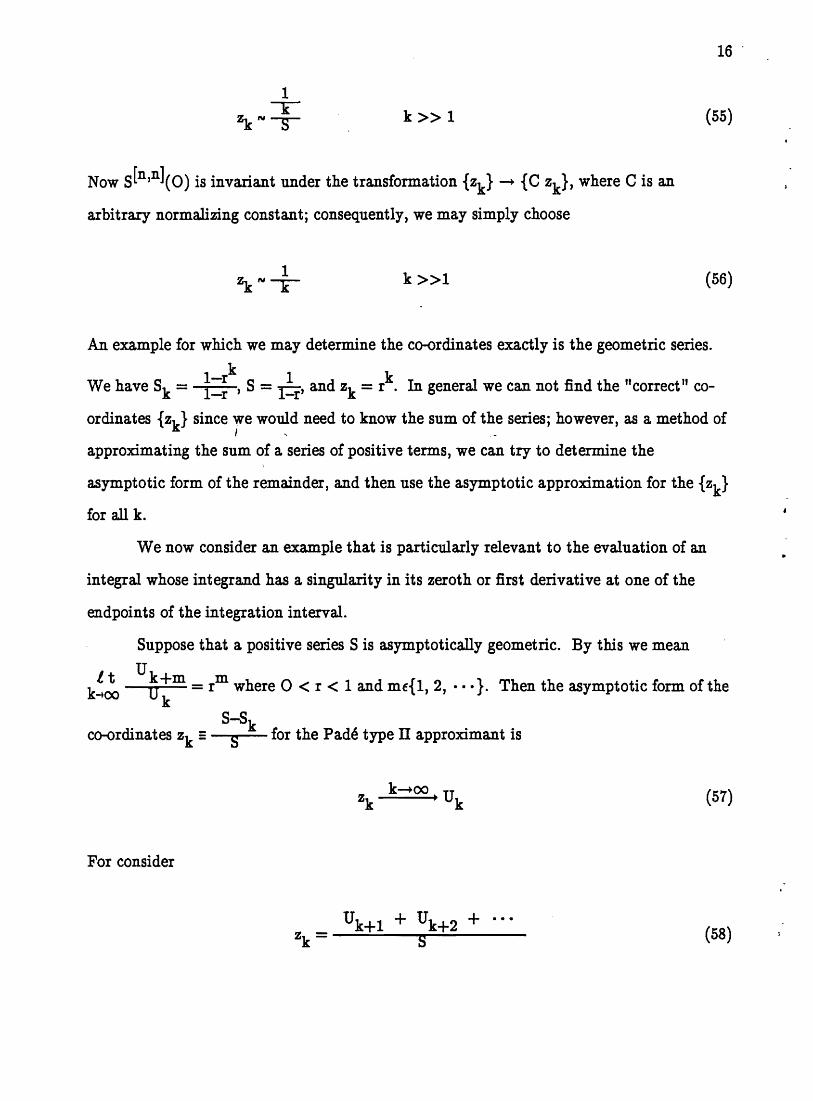


![Approximants in Urdu Language - Center for Language ... in Urdu... · Urdu language, like Korean language has three approximants i.e. [r], [l] and [j]. So /w/ is not present in Urdu](https://static.fdocuments.in/doc/165x107/5f0523fe7e708231d411789f/approximants-in-urdu-language-center-for-language-in-urdu-urdu-language.jpg)


![April 1983 Class 1 of Nonideal Solutions, · Margules representation and refer to approximants of the type [n,O] as the general van Larr representation because [1,0] corresponds to](https://static.fdocuments.in/doc/165x107/5e9d3fd0f8a62435b1511631/april-1983-class-1-of-nonideal-solutions-margules-representation-and-refer-to-approximants.jpg)

![Cafe - Publishpublish.uwo.ca/~jnuttall/cafe.pdf · multipoint Pade approximants to certain entire functions, including some of the form exp[polynomial]. The conjecture is very simple](https://static.fdocuments.in/doc/165x107/5c5eb64e09d3f20b6b8c2345/cafe-jnuttallcafepdf-multipoint-pade-approximants-to-certain-entire-functions.jpg)