Package ‘monomvn’ - The Comprehensive R Archive … · Package ‘monomvn ’ January 8, 2017...

Package ‘monomvn’January 8, 2017

Type Package

Title Estimation for Multivariate Normal and Student-t Data withMonotone Missingness

Version 1.9-7

Date 2016-12-28

Author Robert B. Gramacy <[email protected]>

Maintainer Robert B. Gramacy <[email protected]>

Description Estimation of multivariate normal and student-t data ofarbitrary dimension where the pattern of missing data is monotone.Through the use of parsimonious/shrinkage regressions(plsr, pcr, lasso, ridge, etc.), where standard regressions fail,the package can handle a nearly arbitrary amount of missing data.The current version supports maximum likelihood inference anda full Bayesian approach employing scale-mixtures for Gibbs sampling.Monotone data augmentation extends thisBayesian approach to arbitrary missingness patterns.A fully functional standalone interface to the Bayesian lasso(from Park & Casella), Normal-Gamma (from Griffin & Brown),Horseshoe (from Carvalho, Polson, & Scott), and ridge regressionwith model selection via Reversible Jump, and student-t errors(from Geweke) is also provided.

Depends R (>= 2.14.0), pls, lars, MASS

Imports quadprog, mvtnorm

License LGPL

URL http://bobby.gramacy.com/r_packages/monomvn

NeedsCompilation yes

Repository CRAN

Date/Publication 2017-01-08 15:02:13

1

http://bobby.gramacy.com/r_packages/monomvn

2 monomvn-package

R topics documented:monomvn-package . . . . . . . . . . . . . . . . . . . . . . . . . . . . . . . . . . . . . 2blasso . . . . . . . . . . . . . . . . . . . . . . . . . . . . . . . . . . . . . . . . . . . . 3blasso.s3 . . . . . . . . . . . . . . . . . . . . . . . . . . . . . . . . . . . . . . . . . . . 8bmonomvn . . . . . . . . . . . . . . . . . . . . . . . . . . . . . . . . . . . . . . . . . 10cement . . . . . . . . . . . . . . . . . . . . . . . . . . . . . . . . . . . . . . . . . . . . 16default.QP . . . . . . . . . . . . . . . . . . . . . . . . . . . . . . . . . . . . . . . . . . 18metrics . . . . . . . . . . . . . . . . . . . . . . . . . . . . . . . . . . . . . . . . . . . . 21monomvn . . . . . . . . . . . . . . . . . . . . . . . . . . . . . . . . . . . . . . . . . . 23monomvn.s3 . . . . . . . . . . . . . . . . . . . . . . . . . . . . . . . . . . . . . . . . . 27monomvn.solve.QP . . . . . . . . . . . . . . . . . . . . . . . . . . . . . . . . . . . . . 29plot.monomvn . . . . . . . . . . . . . . . . . . . . . . . . . . . . . . . . . . . . . . . . 30randmvn . . . . . . . . . . . . . . . . . . . . . . . . . . . . . . . . . . . . . . . . . . . 31regress . . . . . . . . . . . . . . . . . . . . . . . . . . . . . . . . . . . . . . . . . . . . 33returns . . . . . . . . . . . . . . . . . . . . . . . . . . . . . . . . . . . . . . . . . . . . 36rmono . . . . . . . . . . . . . . . . . . . . . . . . . . . . . . . . . . . . . . . . . . . . 38rwish . . . . . . . . . . . . . . . . . . . . . . . . . . . . . . . . . . . . . . . . . . . . 39

Index 40

monomvn-package Estimation for Multivariate Normal and Student-t Data with Mono-tone Missingness

Description

Estimation of multivariate normal and student-t data of arbitrary dimension where the pattern ofmissing data is monotone. Through the use of parsimonious/shrinkage regressions (plsr, pcr, lasso,ridge, etc.), where standard regressions fail, the package can handle a nearly arbitrary amount ofmissing data. The current version supports maximum likelihood inference and a full Bayesianapproach employing scale-mixtures for Gibbs sampling. Monotone data augmentation extends thisBayesian approach to arbitrary missingness patterns. A fully functional standalone interface to theBayesian lasso (from Park & Casella), the Normal-Gamma (from Griffin & Brown), Horseshoe(from Carvalho, Polson, & Scott), and ridge regression with model selection via Reversible Jump,and student-t errors (from Geweke) is also provided

Details

For a fuller overview including a complete list of functions, demos and vignettes, please usehelp(package="monomvn").

Author(s)

Robert B. Gramacy <[email protected]>

Maintainer: Robert B. Gramacy <[email protected]>

blasso 3

References

Robert B. Gramacy, Joo Hee Lee and Ricardo Silva (2008). On estimating covariances betweenmany assets with histories of highly variable length.Preprint available on arXiv:0710.5837: http://arxiv.org/abs/0710.5837


See Also

monomvn, the now defunct norm package, mvnmle

blasso Bayesian Lasso/NG, Horseshoe, and Ridge Regression

Description

Inference for ordinary least squares, lasso/NG, horseshoe and ridge regression models by (Gibbs)sampling from the Bayesian posterior distribution, augmented with Reversible Jump for modelselection

Usage

bhs(X, y, T=1000, thin=NULL, RJ=TRUE, M=NULL, beta=NULL,lambda2=1, s2=var(y-mean(y)), mprior=0, ab=NULL,theta=0, rao.s2=TRUE, icept=TRUE, normalize=TRUE, verb=1)

bridge(X, y, T = 1000, thin = NULL, RJ = TRUE, M = NULL,beta = NULL, lambda2 = 1, s2 = var(y-mean(y)), mprior = 0,rd = NULL, ab = NULL, theta=0, rao.s2 = TRUE, icept = TRUE,normalize = TRUE, verb = 1)

blasso(X, y, T = 1000, thin = NULL, RJ = TRUE, M = NULL,beta = NULL, lambda2 = 1, s2 = var(y-mean(y)),case = c("default", "ridge", "hs", "ng"), mprior = 0, rd = NULL,ab = NULL, theta = 0, rao.s2 = TRUE, icept = TRUE,normalize = TRUE, verb = 1)

Arguments

X data.frame, matrix, or vector of inputs X

y vector of output responses y of length equal to the leading dimension (rows) ofX, i.e., length(y) == nrow(X)

T total number of MCMC samples to be collected

thin number of MCMC samples to skip before a sample is collected (via thinning). IfNULL (default), then thin is determined based on the regression model impliedby RJ, lambda2, and ncol(X); and also on the errors model implied by thetaand nrow(X)

http://arxiv.org/abs/0710.5837


4 blasso

RJ if TRUE then model selection on the columns of the design matrix (and thus theparameter beta in the model) is performed by Reversible Jump (RJ) MCMC.The initial model is specified by the beta input, described below, and the maxi-mal number of covariates in the model is specified by M

M the maximal number of allowed covariates (columns of X) in the model. If in-put lambda2 > 0 then any M <= ncol(X) is allowed. Otherwise it must bethat M <= min(ncol(X), length(y)-1), which is default value when a NULLargument is given

beta initial setting of the regression coefficients. Any zero-components will implythat the corresponding covariate (column of X) is not in the initial model. Wheninput RJ = FALSE (no RJ) and lambda2 > 0 (use lasso) then no compo-nents are allowed to be exactly zero. The default setting is therefore contextual;see below for details

lambda2 square of the initial lasso penalty parameter. If zero, then least squares regres-sions are used

s2 initial variance parametercase specifies if ridge regression, the Normal-Gamma, or the horseshoe prior should

be done instead of the lasso; only meaningful when lambda2 > 0

mprior prior on the number of non-zero regression coefficients (and therefore covari-ates) m in the model. The default (mprior = 0) encodes the uniform prior on0 <= m <= M. A scalar value 0 < mprior < 1 implies a Binomial priorBin(m|n=M,p=mprior). A 2-vector mprior=c(g,h) of positive values g and hrepresents gives Bin(m|n=M,p) prior where p~Beta(g,h)

rd =c(r, delta), the alpha (shape) parameter and β (rate) parameter to the gammadistribution prior G(r,delta) for the λ2 parameter under the lasso model; or,the α (shape) parameter and β (scale) parameter to the inverse-gamma distribu-tion IG(r/2, delta/2) prior for the λ2 parameter under the ridge regressionmodel. A default of NULL generates appropriate non-informative values depend-ing on the nature of the regression. Specifying rd=FALSE causes lambda2 valuesto be fixed at their starting value, i.e., not sampled. See the details below for in-formation on the special settings for ridge regression

ab =c(a, b), the α (shape) parameter and the β (scale) parameter for the inverse-gamma distribution prior IG(a,b) for the variance parameter s2. A default ofNULL generates appropriate non-informative values depending on the nature ofthe regression

theta the rate parameter (> 0) to the exponential prior on the degrees of freedomparamter nu under a model with Student-t errors implemented by a scale-mixtureprior. The default setting of theta = 0 turns off this prior, defaulting to a normalerrors prior

rao.s2 indicates whether Rao-Blackwellized samples for σ2 should be used (defaultTRUE); see below for more details

icept if TRUE, an implicit intercept term is fit in the model, otherwise the the interceptis zero; default is TRUE

normalize if TRUE, each variable is standardized to have unit L2-norm, otherwise it is leftalone; default is TRUE

verb verbosity level; currently only verb = 0 and verb = 1 are supported

blasso 5

Details

The Bayesian lasso model and Gibbs Sampling algorithm is described in detail in Park & Casella(2008). The algorithm implemented by this function is identical to that described therein, withthe exception of an added “option” to use a Rao-Blackwellized sample of σ2 (with β integratedout) for improved mixing, and the model selections by RJ described below. When input argumentlambda2 = 0 is supplied, the model is a simple hierarchical linear model where (β, σ2) is given aJeffrey’s prior

Specifying RJ = TRUE causes Bayesian model selection and averaging to commence for choosingwhich of the columns of the design matrix X (and thus parameters beta) should be included in themodel. The zero-components of the beta input specify which columns are in the initial model, andM specifies the maximal number of columns.

The RJ mechanism implemented here for the Bayesian lasso model selection differs from the onedescribed by Hans (2009), which is based on an idea from Geweke (1996). Those methods requiredeparting from the Park & Casella (2008) latent-variable model and requires sampling from eachconditional βi|β(−i), . . . for all i, since a mixture prior with a point-mass at zero is placed on eachβi. Out implementation here requires no such special prior and retains the joint sampling from thefull β vector of non-zero entries, which we believe yields better mixing in the Markov chain. RJproposals to increase/decrease the number of non-zero entries does proceed component-wise, butthe acceptance rates are high due due to marginalized between-model moves (Troughton & Godsill,1997).

When the lasso prior or RJ is used, the automatic thinning level (unless thin != NULL) is deter-mined by the number of columns of X since this many latent variables are introduced

Bayesian ridge regression is implemented as a special case via the bridge function. This essentiallycalls blasso with case = "ridge". A default setting of rd = c(0,0) is implied by rd = NULL,giving the Jeffery’s prior for the penalty parameter λ2 unless ncol(X) >= length(y) in whichcase the proper specification of rd = c(5,10) is used instead.

The Normal–Gamma prior (Griffin & Brown, 2009) is implemented as an extension to the Bayesianlasso with case = "ng". Many thanks to James Scott for providing the code needed to extend themethod(s) to use the horseshoe prior (Carvalho, Polson, Scott, 2010).

When theta > 0 then the Student-t errors via scale mixtures (and thereby extra latent variablesomega2) of Geweke (1993) is applied as an extension to the Bayesian lasso/ridge model. If Student-terrors are used the automatic thinning level is augmented (unless thin != NULL) by the number ofrows in X since this many latent variables are introduced

Value

blasso returns an object of class "blasso", which is a list containing a copy of all of the inputarguments as well as of the components listed below.

call a copy of the function call as used

mu a vector of T samples of the (un-penalized) “intercept” parameter

beta a T*ncol(X) matrix of T samples from the (penalized) regression coefficients

m the number of non-zero entries in each vector of T samples of beta

s2 a vector of T samples of the variance parameter

lambda2 a vector of T samples of the penalty parameter

6 blasso

gamma a vector of T with the gamma parameter when case = "ng"

tau2i a T*ncol(X) matrix of T samples from the (latent) inverse diagonal of the priorcovariance matrix for beta, obtained for Lasso regressions

omega2 a T*nrow(X) matrix of T samples from the (latent) diagonal of the covariancematrix of the response providing a scale-mixture implementation of Student-terrors with degrees of freedom nu when active (input theta > 0)

nu a vector of T samples of the degrees of freedom parameter to the Student-t errorsmode when active (input theta > 0)

pi a vector of T samples of the Binomial proportion p that was given a Beta prior,as described above for the 2-vector version of the mprior input

lpost the log posterior probability of each (saved) sample of the joint parameters

llik the log likelihood of each (saved) sample of the parameters

llik.norm the log likelihood of each (saved) sample of the parameters under the Normalerrors model when sampling under the Student-t model; i.e., it is not presentunless theta > 0

Note

Whenever ncol(X) >= nrow(X) it must be that either RJ = TRUE with M <= nrow(X)-1 (thedefault) or that the lasso is turned on with lambda2 > 0. Otherwise the regression problem isill-posed.

Since the starting values are considered to be first sample (of T), the total number of (new) samplesobtained by Gibbs Sampling will be T-1

Author(s)


References

Park, T., Casella, G. (2008). The Bayesian Lasso.Journal of the American Statistical Association, 103(482), June 2008, pp. 681-686http://www.stat.ufl.edu/~casella/Papers/Lasso.pdf

Griffin, J.E. and Brown, P.J. (2009). Inference with Normal-Gamma prior distributions in regressionproblems. Bayesian Analysis, 5, pp. 171-188.http://projecteuclid.org/euclid.ba/1340369797

Hans, C. (2009). Bayesian Lasso regression. Biometrika 96, pp. 835-845.http://biomet.oxfordjournals.org/content/96/4/835.abstract

Carvalho, C.M., Polson, N.G., and Scott, J.G. (2010) The horseshoe estimator for sparse signals.Biometrika 97(2): pp. 465-480.http://ftp.stat.duke.edu/WorkingPapers/08-31.pdf

Geweke, J. (1996). Variable selection and model comparison in regression. In Bayesian Statistics5. Editors: J.M. Bernardo, J.O. Berger, A.P. Dawid and A.F.M. Smith, 609-620. Oxford Press.

Paul T. Troughton and Simon J. Godsill (1997). A reversible jump sampler for autoregressivetime series, employing full conditionals to achieve efficient model space moves. Technical ReportCUED/F-INFENG/TR.304, Cambridge University Engineering Department.

http://www.stat.ufl.edu/~casella/Papers/Lasso.pdf

http://projecteuclid.org/euclid.ba/1340369797

http://biomet.oxfordjournals.org/content/96/4/835.abstract

http://ftp.stat.duke.edu/WorkingPapers/08-31.pdf

blasso 7

Geweke, J. (1993) Bayesian treatment of the independent Student-t linear model. Journal of AppliedEconometrics, Vol. 8, S19-S40


See Also

lm , lars in the lars package, regress, lm.ridge in the MASS package

Examples

## following the lars diabetes exampledata(diabetes)attach(diabetes)

## Ordinary Least Squares regressionreg.ols <- regress(x, y)

## Lasso regressionreg.las <- regress(x, y, method="lasso")

## Bayesian Lasso regressionreg.blas <- blasso(x, y)

## summarize the beta (regression coefficients) estimatesplot(reg.blas, burnin=200)points(drop(reg.las$b), col=2, pch=20)points(drop(reg.ols$b), col=3, pch=18)legend("topleft", c("blasso-map", "lasso", "lsr"),

col=c(2,2,3), pch=c(21,20,18))

## plot the size of different models visitedplot(reg.blas, burnin=200, which="m")

## get the summarys <- summary(reg.blas, burnin=200)

## calculate the probability that each beta coef != zeros$bn0

## summarize s2plot(reg.blas, burnin=200, which="s2")s$s2

## summarize lambda2plot(reg.blas, burnin=200, which="lambda2")s$lambda2

## Not run:## fit with Student-t errors## (~400-times slower due to automatic thinning level)regt.blas <- blasso(x, y, theta=0.1)


8 blasso.s3

## plotting some information about nu, and quantilesplot(regt.blas, "nu", burnin=200)quantile(regt.blas$nu[-(1:200)], c(0.05, 0.95))

## Bayes Factor shows strong evidence for Student-t modelmean(exp(regt.blas$llik[-(1:200)] - regt.blas$llik.norm[-(1:200)]))

## End(Not run)

## clean updetach(diabetes)

blasso.s3 Summarizing Bayesian Lasso Output

Description

Summarizing, printing, and plotting the contents of a "blasso"-class object containing samplesfrom the posterior distribution of a Bayesian lasso model

Usage

## S3 method for class 'blasso'print(x, ...)## S3 method for class 'blasso'summary(object, burnin = 0, ...)## S3 method for class 'blasso'plot(x, which=c("coef", "s2", "lambda2", "gamma",

"tau2i","omega2", "nu", "m", "pi"), subset = NULL, burnin = 0,... )

## S3 method for class 'summary.blasso'print(x, ...)

Arguments

object a "blasso"-class object that must be named object for the generic methodssummary.blasso

x a "blasso"-class object that must be named x for the generic printing and plot-ting methods print.summary.blasso and plot.blasso

subset a vector of indicies that can be used to specify the a subset of the columns oftau2i or omega2 that are plotted as boxplots in order to reduce clutter

burnin number of burn-in rounds to discard before reporting summaries and makingplots. Must be non-negative and less than x$T

which indicates the parameter whose characteristics should be plotted; does not applyto the summary

... passed to print.blasso, or plot.default

blasso.s3 9

Details

print.blasso prints the call followed by a brief summary of the MCMC run and a suggestion totry the summary and plot commands.

plot.blasso uses an appropriate plot command on the list entries of the "blasso"-class objectthus visually summarizing the samples from the posterior distribution of each parameter in themodel depending on the which argument supplied.

summary.blasso uses the summary command on the list entries of the "blasso"-class object thussummarizing the samples from the posterior distribution of each parameter in the model.

print.summary.monomvn calls print.blasso on the object and then prints the result of summary.blasso

Value

summary.blasso returns a "summary.blasso"-class object, which is a list containing (a subsetof) the items below. The other functions do not return values.

B a copy of the input argument thin

T total number of MCMC samples to be collected from x$T

thin number of MCMC samples to skip before a sample is collected (via thinning)from x$T

coef a joint summary of x$mu and the columns of x$beta, the regression coefficients

s2 a summary of x$s2, the variance parameter

lambda2 a summary of x$lambda2, the penalty parameter, when lasso or ridge regressionis active

lambda2 a summary of x$gamma, when the NG extensions to the lasso are used

tau2i a summary of the columns of the latent x$tau2i parameters when lasso is active

omega2 a summary of the columns of the latent x$omega2 parameters when Student-terrors are active

nu a summary of x$nu, the degrees of freedom parameter, when the Student-t modelis active

bn0 the estimated posterior probability that the individual components of the regres-sion coefficients beta is nonzero

m a summary the model order x$m: the number of non-zero regression coefficientsbeta

pi the estimated Binomial proportion in the prior for the model order when 2-vectorinput is provided for mprior

Author(s)


References



10 bmonomvn

See Also

blasso

bmonomvn Bayesian Estimation for Multivariate Normal Data with MonotoneMissingness

Description

Bayesian estimation via sampling from the posterior distribution of the of the mean and covariancematrix of multivariate normal (MVN) distributed data with a monotone missingness pattern, viaGibbs Sampling. Through the use of parsimonious/shrinkage regressions (lasso/NG & ridge), wherestandard regressions fail, this function can handle an (almost) arbitrary amount of missing data

Usage

bmonomvn(y, pre = TRUE, p = 0.9, B = 100, T = 200, thin = 1,economy = FALSE, method = c("lasso", "ridge", "lsr", "factor","hs", "ng"), RJ = c("p", "bpsn", "none"), capm = TRUE,start = NULL, mprior = 0, rd = NULL, theta = 0, rao.s2 = TRUE,QP = NULL, verb = 1, trace = FALSE)

Arguments

y data matrix were each row is interpreted as a random sample from a MVNdistribution with missing values indicated by NA

pre logical indicating whether pre-processing of the y is to be performed. This sortsthe columns so that the number of NAs is non-decreasing with the column index

p when performing regressions, p is the proportion of the number of columns torows in the design matrix before an alternative regression (lasso, ridge, or RJ) isperformed as if least-squares regression has “failed”. Least-squares regressionis known to fail when the number of columns equals the number of rows, hencea default of p = 0.9 <= 1. Alternatively, setting p = 0 forces a parsimoniousmethod to be used for every regression. Intermediate settings of p allow theuser to control when least-squares regressions stop and the parsimonious onesstart; When method = "factor" the p argument represents an integer (positive)number of initial columns of y to treat as known factors

B number of Burn-In MCMC sampling rounds, during which samples are dis-carded

T total number of MCMC sampling rounds to take place after burn-in, duringwhich samples are saved

thin multiplicative thinning in the MCMC. Each Bayesian (lasso) regression will dis-card thin*M MCMC rounds, where M is the number of columns in its design ma-trix, before a sample is saved as a draw from the posterior distribution; Likewiseif theta != 0 a further thin*N, for N responses will be discarded

bmonomvn 11

economy indicates whether memory should be economized at the expense of speed. WhenTRUE the individual Bayesian (lasso) regressions are cleaned between uses sothat only one of them has a large footprint at any time during sampling from theMarkov chain. When FALSE (default) all regressions are pre-allocated and thefull memory footprint is realized at the outset, saving dynamic allocations

method indicates the Bayesian parsimonious regression specification to be used, choos-ing between the lasso (default) of Park \& Casella, the NG extension, the horse-shoe, a ridge regression special case, and least-squares. The "factor" methodtreats the first p columns of y as known factors

RJ indicates the Reversible Jump strategy to be employed. The default argument of"p" method uses RJ whenever a parsimonious regression is used; "bpsn" onlyuses RJ for regressions with p >= n, and "none" never uses RJ

capm when TRUE this argument indicates that the number of components of β shouldnot exceed n, the number of response variables in a particular regression

start a list depicting starting values for the parameters that are use to initialize theMarkov chain. Usually this will be a "monomvn"-class object depicting maxi-mum likelihood estimates output from the monomvn function. The relevant fieldsare the mean vector $mu, covariance matrix $S, monotone ordering $o (for sanitychecking with input y), component vector $ncomp and penalty parameter vector$lambda; see note below

mprior prior on the number of non-zero regression coefficients (and therefore covari-ates) m in the model. The default (mprior = 0) encodes the uniform prior on0 < m < M. A scalar value 0 <= mprior <= 1 implies a Binomial priorBin(m|n=M,p=mprior). A 2-vector mprior=c(g,h) of positive values g and hrepresents gives Bin(m|n=M,p) prior where p~Beta(g,h)

rd =c(r,delta); a 2-vector of prior parameters for λ2 which depends on the re-gression method. When method = "lasso" then the components arethe α (shape) and β (rate) parameters to the a gamma distribution G(r,delta);when method = "ridge" the components are the α (shape) and β (scale) pa-rameters to an inverse-gamma distribution IG(r/2,delta/2)

theta the rate parameter (> 0) to the exponential prior on the degrees of freedomparamter nu for each regression model implementing Student-t errors (for eachcolumn of Y marginally) by a scale-mixture prior. See blasso for more details.The default setting of theta = 0 turns off this prior, defaulting to a normalerrors prior. A negative setting triggers a pooling of the degrees of freedomparameter across all columns of Y. I.e., Y is modeled as multivariate-t. In thiscase abs{theta} is used as the prior parameterization

rao.s2 indicates whether to Rao-Blackwellized samples for σ2 should be used (defaultTRUE); see the details section of blasso for more information

QP if non-NULL this argument should either be TRUE, a positive integer, or containa list specifying a Quadratic Program to solve as a function of the samples ofmu = dvec and Sigma = Dmat in the notation of solve.QP; see default.QPfor a default specification that is used when QP = TRUE or a positive integer isis given; more details are below

verb verbosity level; currently only verb = 0 and verb = 1 are supported

12 bmonomvn

trace if TRUE then samples from all parameters are saved to files in the CWD, and thenread back into the "monomvn"-class object upon return

Details

If pre = TRUE then bmonomvn first re-arranges the columns of y into nondecreasing order withrespect to the number of missing (NA) entries. Then (at least) the first column should be completelyobserved.

Samples from the posterior distribution of the MVN mean vector and covariance matrix are ob-tained sampling from the posterior distribution of Bayesian regression models. The methodologyfor converting these to samples from the mean vector and covariance matrix is outlined in themonomvn documentation, detailing a similarly structured maximum likelihood approach. Also seethe references below.

Whenever the regression model is ill–posed (i.e., when there are more covariates than responses,or a “big p small n” problem) then Bayesian lasso or ridge regressions – possibly augmented withReversible Jump (RJ) for model selection – are used instead. See the Park \& Casella referencebelow, and the blasso documentation. To guarantee each regression is well posed the combinationsetting of method="lsr" and RJ="none" is not allowed. As in monomvn the p argument can beused to turn on lasso or ridge regressions (possibly with RJ) at other times. The exception is the"factor" method which always involves an OLS regression on (a subset of) the first p columns ofy.

Samples from a function of samples of mu and Sigma can be obtained by specifying a Quadraticprogram via the argument QP. The idea is to allow for the calculation of the distribution of minimumvariance and mean–variance portfolios, although the interface is quite general. See default.QP formore details, as default.QP(ncol(y)) is used when the argument QP = TRUE is given. When apositive integer is given, then the first QP columns of y are treated as factors by using

default.QP(ncol(y) - QP)

instead. The result is that the corresponding components of (samples of) mu and rows/cols of S arenot factored into the specification of the resulting Quadratic Program

Value

bmonomvn returns an object of class "monomvn", which is a list containing the inputs above and asubset of the components below.


mu estimated mean vector with columns corresponding to the columns of y

S estimated covariance matrix with rows and columns corresponding to the columnsof y

mu.var estimated variance of the mean vector with columns corresponding to the columnsof y

mu.cov estimated covariance matrix of the mean vector with columns corresponding tothe columns of y

S.var estimated variance of the individual components of the covariance matrix withcolumns and rows corresponding to the columns of y

bmonomvn 13

mu.map estimated maximum a’ posteriori (MAP) of the mean vector with columns cor-responding to the columns of y

S.map estimated MAP of the individual components of the covariance matrix withcolumns and rows corresponding to the columns of y

S.nz posterior probability that the individual entries of the covariance matrix are non–zero

Si.nz posterior probability that the individual entries of the inverse of the covariancematrix are non–zero

nu when theta < 0 this field provides a trace of the pooled nu parameter to themultivariate-t distribution

lpost.map log posterior probability of the MAP estimate

which.map gives the time index of the sample corresponding to the MAP estimate

llik a trace of the log likelihood of the data

llik.norm a trace of the log likelihood under the Normal errors model when sampling underthe Student-t model; i.e., it is not present unless theta > 0. Used for calculatingBayes Factors

na when pre = TRUE this is a vector containing number of NA entries in eachcolumn of y

o when pre = TRUE this is a vector containing the index of each column in thesorting of the columns of y obtained by o <- order(na)

method method of regression used on each column, or "bcomplete" indicating that noregression was used

thin the (actual) number of thinning rounds used for the regression (method) in eachcolumn

lambda2 records the mean λ2 value found in the trace of the Bayesian Lasso regressions.Zero-values result when the column corresponds to a complete case or an ordi-nary least squares regression (these would be NA entries from monomvn)

ncomp records the mean number of components (columns of the design matrix) used inthe regression model for each column of y. If input RJ = FALSE then this simplycorresponds to the monotone ordering (these would correspond to the NA entriesfrom monomvn). When RJ = TRUE the monotone ordering is an upper bound (oneach entry)

trace if input trace = TRUE then this field contains traces of the samples of µ in thefield $mu and of Σ in the field $S, and of all regression parameters for each ofthe m = length(mu) columns in the field $reg. This $reg field is a stripped-down "blasso"-class object so that the methods of that object may be used foranalysis. If data augmentation is required to complete the monotone missingnesspattern, then samples from these entries of Y are contained in $DA where thecolumn names indicate the i-j entry of Y sampled; see the R output below

R gives a matrix version of the missingness pattern used: 0-entries mean ob-served; 1-entries indicate missing values conforming to a monotone pattern;2-entries indicate missing values that require data augmentation to complete amonotone missingness pattern

14 bmonomvn

B from inputs: number of Burn-In MCMC sampling rounds, during which samplesare discarded

T from inputs: total number of MCMC sampling rounds to take place after burn-in, during which samples are saved

r from inputs: alpha (shape) parameter to the gamma distribution prior for thelasso parameter lambda

delta from inputs: beta (rate) parameter to the gamma distribution prior for the lassoparameter lambda

QP if a valid (non–FALSE or NULL) QP argument is given, then this field contains thespecification of a Quadratic Program in the form of a list with entries includ-ing $dvec, $Amat, $b0, and $meq, similar to the usage in solve.QP, and someothers; see default.QP for more details

W when input QP = TRUE is given, then this field contains a T*ncol(y) matrix ofsamples from the posterior distribution of the solution to the Quadratic Program,which can be visualized via plot.monomvn using the argument which = "QP"

Note

Whenever the bmonomvn algorithm requires a regression where p >= n, i.e., if any of the columns inthe y matrix have fewer non–NA elements than the number of columns with more non–NA elements,then it is helpful to employ both lasso/ridge and the RJ method.

It is important that any starting values provided in the start be compatible with the regressionmodel specified by inputs RJ and method. Any incompatibilities will result with a warning that(alternative) default action was taken and may result in an undesired (possibly inferior) model beingfit

Author(s)


References

R.B. Gramacy and E. Pantaleo (2010). Shrinkage regression for multivariate inference with missingdata, and an application to portfolio balancing. Preprint available on arXiv:0710.5837 http://arxiv.org/abs/0907.2135

Roderick J.A. Little and Donald B. Rubin (2002). Statistical Analysis with Missing Data, SecondEdition. Wilely.


See Also

blasso, monomvn, default.QP, em.norm in the now defunct norm and mvnmle packages, andreturns




bmonomvn 15

Examples

## standard usage, duplicating the results in## Little and Rubin, section 7.4.3data(cement.miss)out <- bmonomvn(cement.miss)outout$muout$S

#### A bigger example, comparing the various## parsimonious methods##

## generate N=100 samples from a 10-d random MVNxmuS <- randmvn(100, 20)

## randomly impose monotone missingnessxmiss <- rmono(xmuS$x)

## using least squares only when necessary,obl <- bmonomvn(xmiss)obl

## look at the posterior variabilitypar(mfrow=c(1,2))plot(obl)plot(obl, "S")

## compare to maximum likelihoodEllik.norm(obl$mu, obl$S, xmuS$mu, xmuS$S)oml <- monomvn(xmiss, method="lasso")Ellik.norm(oml$mu, oml$S, xmuS$mu, xmuS$S)

#### a min-variance portfolio allocation example##

## get the returns data, and use 20 random colsdata(returns)train <- returns[,sample(1:ncol(returns), 20)]

## missingness pattern requires DA; also gather## samples from the solution to a QPobl.da <- bmonomvn(train, p=0, QP=TRUE)

## plot the QP weights distributionplot(obl.da, "QP", xaxis="index")

## get ML solution: will warn about monotone violationssuppressWarnings(oml.da <- monomvn(train, method="lasso"))

16 cement

## add mean and MLE comparison, requires the## quadprog library for the solve.QP functionadd.pe.QP(obl.da, oml.da)

## now consider adding in the market as a factordata(market)mtrain <- cbind(market, train)

## fit the model using only factor regressionsobl.daf <- bmonomvn(mtrain, method="factor", p=1, QP=1)plot(obl.daf, "QP", xaxis="index", main="using only factors")suppressWarnings(oml.daf <- monomvn(mtrain, method="factor"))add.pe.QP(obl.daf, oml.daf)

#### a Bayes/MLE comparison using least squares sparingly##

## fit Bayesian and classical lassoobls <- bmonomvn(xmiss, p=0.25)Ellik.norm(obls$mu, obls$S, xmuS$mu, xmuS$S)omls <- monomvn(xmiss, p=0.25, method="lasso")Ellik.norm(omls$mu, omls$S, xmuS$mu, xmuS$S)

## compare to ridge regressionobrs <- bmonomvn(xmiss, p=0.25, method="ridge")Ellik.norm(obrs$mu, obrs$S, xmuS$mu, xmuS$S)omrs <- monomvn(xmiss, p=0.25, method="ridge")Ellik.norm(omrs$mu, omrs$S, xmuS$mu, xmuS$S)

## using the maximum likelihood solution to initialize## the Markov chain and avoid burn-in.ob2s <- bmonomvn(xmiss, p=0.25, B=0, start=omls, RJ="p")Ellik.norm(ob2s$mu, ob2s$S, xmuS$mu, xmuS$S)

cement Hald’s Cement Data

Description

Heat evolved in setting of cement, as a function of its chemical composition.

Usage

data(cement)data(cement.miss)

cement 17

Format

A data.frame with 13 observations on the following 5 variables.

x1 percentage weight in clinkers of 3CaO.Al2O3

x2 percentage weight in clinkers of 3CaO.SiO2

x3 percentage weight in clinkers of 4CaO.Al2O3.Fe2O3

x4 percentage weight in clinkers of 2CaO.SiO2

y heat evolved (calories/gram)

Details

cement.miss is taken from an example in Little & Rubin’s book on Statistical Analysis with Miss-ing Data (2002), pp.~154, for demonstrating estimation of multivariate means and variances whenthe missing data pattern is monotone. These are indicated by NA in cement.miss. See the examplessection of monomvn for a re-working of the example from the textbook

Source

Woods, H., Steinour, H. H. and Starke, H. R. (1932) Effect of composition of Portland cement onheat evolved during hardening. Industrial Engineering and Chemistry, 24, 1207–1214.

References

Davison, A. C. (2003) Statistical Models. Cambridge University Press. Page 355.

Draper, N.R. and Smith, H. (1998) Applied Regression Analysis. Wiley. Page 630.

Roderick J.A. Little and Donald B. Rubin (2002). Statistical Analysis with Missing Data, SecondEdition. Wilely. Page 154.


See Also

monomvn – Several other R packages also include this data set

Examples

data(cement)lm(y~x1+x2+x3+x4,data=cement)


18 default.QP

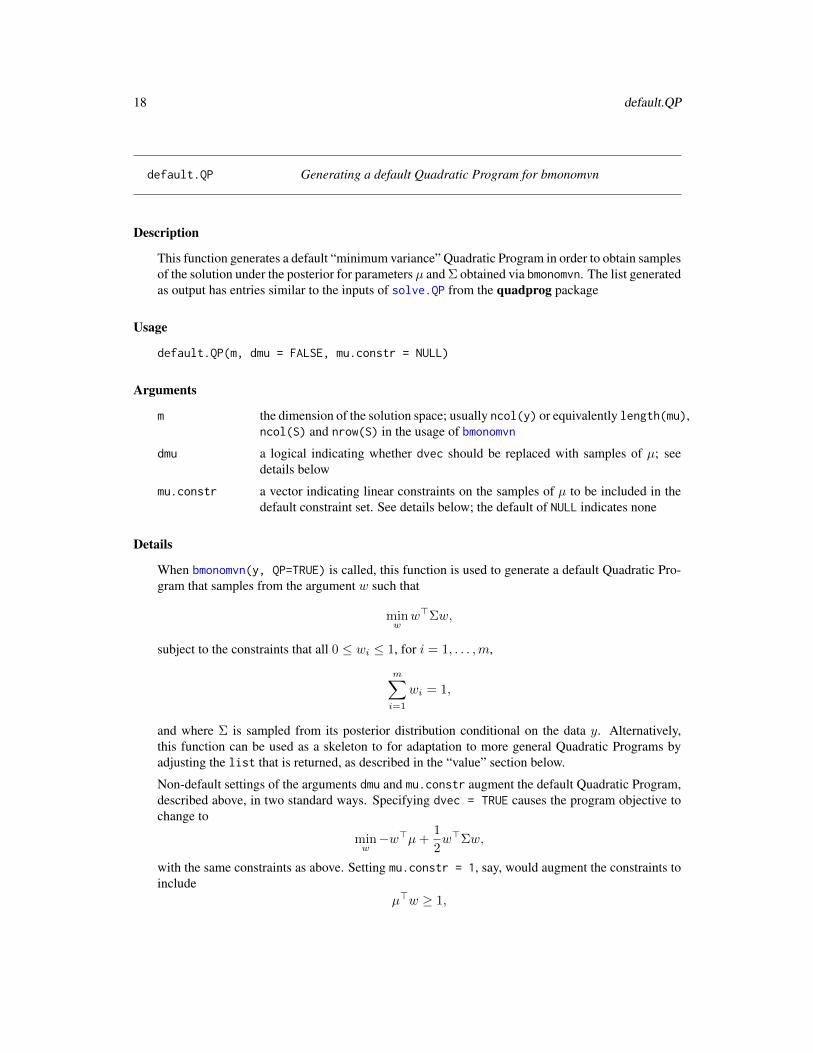
default.QP Generating a default Quadratic Program for bmonomvn

Description

This function generates a default “minimum variance” Quadratic Program in order to obtain samplesof the solution under the posterior for parameters µ and Σ obtained via bmonomvn. The list generatedas output has entries similar to the inputs of solve.QP from the quadprog package

Usage

default.QP(m, dmu = FALSE, mu.constr = NULL)

Arguments

m the dimension of the solution space; usually ncol(y) or equivalently length(mu),ncol(S) and nrow(S) in the usage of bmonomvn

dmu a logical indicating whether dvec should be replaced with samples of µ; seedetails below

mu.constr a vector indicating linear constraints on the samples of µ to be included in thedefault constraint set. See details below; the default of NULL indicates none

Details

When bmonomvn(y, QP=TRUE) is called, this function is used to generate a default Quadratic Pro-gram that samples from the argument w such that

minww>Σw,

subject to the constraints that all 0 ≤ wi ≤ 1, for i = 1, . . . ,m,

m∑i=1

wi = 1,

and where Σ is sampled from its posterior distribution conditional on the data y. Alternatively,this function can be used as a skeleton to for adaptation to more general Quadratic Programs byadjusting the list that is returned, as described in the “value” section below.

Non-default settings of the arguments dmu and mu.constr augment the default Quadratic Program,described above, in two standard ways. Specifying dvec = TRUE causes the program objective tochange to

minw−w>µ+

1

2w>Σw,

with the same constraints as above. Setting mu.constr = 1, say, would augment the constraints toinclude

µ>w ≥ 1,

default.QP 19

for samples of µ from the posterior. Setting mu.constr = c(1,2) would augment the constraintsstill further with

−µ>w ≥ −2,

i.e., with alternating sign on the linear part, so that each sample of µ>w must lie in the interval [1,2].So whereas dmu = TRUE allows the mu samples to enter the objective in a standard way, mu.constr(!= NULL) allows it to enter the constraints.

The accompanying function monomvn.solve.QP can act as an interface between the constructed(default) QP object, and estimates of the covariance matrix Σ and mean vector µ, that is identical tothe one used on the posterior-sample version implemented in bmonomvn. The example below, andthose in the documentation for bmonomvn, illustrate how this feature may be used to extract meanand MLE solutions to the constructed Quadratic Program

Value

This function returns a list that can be interpreted as specifying the following arguments to thesolve.QP function in the quadprog package. See solve.QP for more information of the generalspecification of these arguments. In what follows we simply document the defaults provided bydefault.QP. Note that the Dmat argument is not, specified as bmonomvn will use samples from S(from the posterior) instead

m length(dvec), etc.

dvec a zero-vector rep(0, m), or a one-vector rep(1, m) when dmu = TRUE as thereal dvec that will be used by solve.QP will then be dvec * mu

dmu a copy of the dmu input argument

Amat a matrix describing a linear transformation which, together with b0 and meq,describe the constraint that the components of the sampled solution(s), w, mustbe positive and sum to one

b0 a vector containing the (RHS of) in/equalities described by the these constraints

meq an integer scalar indicating that the first meq constraints described by Amat andb0 are equality constraints; the rest are >=

mu.constr a vector whose length is one greater than the input argument of the same name,providing bmonomvn with the numbermu.constr[1] = length(mu.constr[-1])

and location mu.constr[-1] of the columns of Amat which require multiplica-tion by samples of mu

The $QP object that is returned from bmonomvn will have the following additional field

o an integer vector of length m indicating the ordering of the rows of $Amat, andthus the rows of solutions $W that was used in the monotone factorization of thelikelihood. This field appears only after bmonomvn returns a QP object checkedby the internal function check.QP

Author(s)


20 default.QP

See Also

bmonomvn and solve.QP in the quadprog package, monomvn.solve.QP

Examples

## generate N=100 samples from a 10-d random MVN## and randomly impose monotone missingnessxmuS <- randmvn(100, 20)xmiss <- rmono(xmuS$x)

## set up the minimum-variance (default) Quadratic Program## and sample from the posterior of the solution spaceqp1 <- default.QP(ncol(xmiss))obl1 <- bmonomvn(xmiss, QP=qp1)bm1 <- monomvn.solve.QP(obl1$S, qp1) ## calculate meanbm1er <- monomvn.solve.QP(obl1$S + obl1$mu.cov, qp1) ## use estimation riskoml1 <- monomvn(xmiss)mm1 <- monomvn.solve.QP(oml1$S, qp1) ## calculate MLE

## now obtain samples from the solution space of the## mean-variance QPqp2 <- default.QP(ncol(xmiss), dmu=TRUE)obl2 <- bmonomvn(xmiss, QP=qp2)bm2 <- monomvn.solve.QP(obl2$S, qp2, obl2$mu) ## calculate meanbm2er <- monomvn.solve.QP(obl2$S + obl2$mu.cov, qp2, obl2$mu) ## use estimation riskoml2 <- monomvn(xmiss)mm2 <- monomvn.solve.QP(oml2$S, qp2, oml2$mu) ## calculate MLE

## now obtain samples from minimum variance solutions## where the mean weighted (samples) are constrained to be## greater oneqp3 <- default.QP(ncol(xmiss), mu.constr=1)obl3 <- bmonomvn(xmiss, QP=qp3)bm3 <- monomvn.solve.QP(obl3$S, qp3, obl3$mu) ## calculate meanbm3er <- monomvn.solve.QP(obl3$S + obl3$mu.cov, qp3, obl3$mu) ## use estimation riskoml3 <- monomvn(xmiss)mm3 <- monomvn.solve.QP(oml3$S, qp3, oml2$mu) ## calculate MLE

## plot a comparisonpar(mfrow=c(3,1))plot(obl1, which="QP", xaxis="index", main="Minimum Variance")points(bm1er, col=4, pch=17, cex=1.5) ## add estimation riskpoints(bm1, col=3, pch=18, cex=1.5) ## add meanpoints(mm1, col=5, pch=16, cex=1.5) ## add MLElegend("topleft", c("MAP", "posterior mean", "ER", "MLE"), col=2:5,

pch=c(21,18,17,16), cex=1.5)plot(obl2, which="QP", xaxis="index", main="Mean Variance")points(bm2er, col=4, pch=17, cex=1.5) ## add estimation riskpoints(bm2, col=3, pch=18, cex=1.5) ## add meanpoints(mm2, col=5, pch=16, cex=1.5) ## add MLEplot(obl3, which="QP", xaxis="index", main="Minimum Variance, mean >= 1")points(bm3er, col=4, pch=17, cex=1.5) ## add estimation risk

metrics 21

points(bm3, col=3, pch=18, cex=1.5) ## add meanpoints(mm3, col=5, pch=16, cex=1.5) ## add MLE

## for a further comparison of samples of the QP solution## w under Bayesian and non-Bayesian monomvn, see the## examples in the bmonomvn help file

metrics RMSE, Expected Log Likelihood and KL Divergence Between TwoMultivariate Normal Distributions

Description

These functions calculate the root-mean-squared-error, the expected log likelihood, and Kullback-Leibler (KL) divergence (a.k.a. distance), between two multivariate normal (MVN) distributionsdescribed by their mean vector and covariance matrix

Usage

rmse.muS(mu1, S1, mu2, S2)Ellik.norm(mu1, S1, mu2, S2, quiet=FALSE)kl.norm(mu1, S1, mu2, S2, quiet=FALSE, symm=FALSE)

Arguments

mu1 mean vector of first (estimated) MVN

S1 covariance matrix of first (estimated) MVN

mu2 mean vector of second (true, baseline, or comparator) MVN

S2 covariance matrix of second (true, baseline, or comparator) MVN

quiet when FALSE (default)

symm when TRUE a symmetrized version of the KL divergence is used; see the notebelow

Details

The root-mean-squared-error is calculated between the entries of the mean vectors, and the upper-triangular part of the covariance matrices (including the diagonal).

The KL divergence is given by the formula:

DKL(N1‖N2) =1

2

(log

(|Σ1||Σ2|

)+ tr

(Σ−11 Σ2

)+ (µ1 − µ2)

>Σ−11 (µ1 − µ2)−N

)where N is length(mu1), and must agree with the dimensions of the other parameters. Note thatthe parameterization used involves swapped arguments compared to some other references, e.g., asprovided by Wikipedia. See note below.

22 metrics

The expected log likelihood can be formulated in terms of the KL divergence. That is, the expectedlog likelihood of data simulated from the normal distribution with parameters mu2 and S2 under theestimated normal with parameters mu1 and S1 is given by

−1

2ln{(2πe)N |Σ2|} −DKL(N1‖N2).

Value

In the case of the expected log likelihood the result is a real number. The RMSE is a positive realnumber. The KL divergence method returns a positive real number depicting the distance betweenthe two normal distributions

Note

The KL-divergence is not symmetric. Therefore

kl.norm(mu1,S1,mu2,S2) != kl.norm(mu2,S2,mu1,S1).

But a symmetric metric can be constructed from

0.5 * (kl.norm(mu1,S1,mu2,S2) + kl.norm(mu2,S2,mu1,S1))

or by using symm = TRUE. The arguments are reversed compared to some other references, likeWikipedia. To match those versions use kl.norm(mu2, S2, mu1, s1)

Author(s)


References


Examples

mu1 <- rnorm(5)s1 <- matrix(rnorm(100), ncol=5)S1 <- t(s1) %*% s1

mu2 <- rnorm(5)s2 <- matrix(rnorm(100), ncol=5)S2 <- t(s2) %*% s2

## RMSErmse.muS(mu1, S1, mu2, S2)

## expected log likelihoodEllik.norm(mu1, S1, mu2, S2)

## KL is not symmetrickl.norm(mu1, S1, mu2, S2)kl.norm(mu2, S2, mu1, S1)


monomvn 23

## symmetric versionkl.norm(mu2, S2, mu1, S1, symm=TRUE)

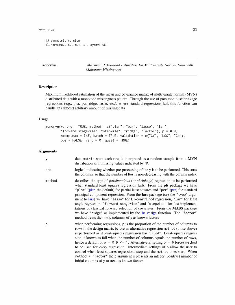
monomvn Maximum Likelihood Estimation for Multivariate Normal Data withMonotone Missingness

Description

Maximum likelihood estimation of the mean and covariance matrix of multivariate normal (MVN)distributed data with a monotone missingness pattern. Through the use of parsimonious/shrinkageregressions (e.g., plsr, pcr, ridge, lasso, etc.), where standard regressions fail, this function canhandle an (almost) arbitrary amount of missing data

Usage

monomvn(y, pre = TRUE, method = c("plsr", "pcr", "lasso", "lar","forward.stagewise", "stepwise", "ridge", "factor"), p = 0.9,ncomp.max = Inf, batch = TRUE, validation = c("CV", "LOO", "Cp"),obs = FALSE, verb = 0, quiet = TRUE)

Arguments

y data matrix were each row is interpreted as a random sample from a MVNdistribution with missing values indicated by NA

pre logical indicating whether pre-processing of the y is to be performed. This sortsthe columns so that the number of NAs is non-decreasing with the column index

method describes the type of parsimonious (or shrinkage) regression to be performedwhen standard least squares regression fails. From the pls package we have"plsr" (plsr, the default) for partial least squares and "pcr" (pcr) for standardprincipal component regression. From the lars package (see the "type" argu-ment to lars) we have "lasso" for L1-constrained regression, "lar" for leastangle regression, "forward.stagewise" and "stepwise" for fast implemen-tations of classical forward selection of covariates. From the MASS packagewe have "ridge" as implemented by the lm.ridge function. The "factor"method treats the first p columns of y as known factors

p when performing regressions, p is the proportion of the number of columns torows in the design matrix before an alternative regression method (those above)is performed as if least-squares regression has “failed”. Least-squares regres-sion is known to fail when the number of columns equals the number of rows,hence a default of p = 0.9 <= 1. Alternatively, setting p = 0 forces methodto be used for every regression. Intermediate settings of p allow the user tocontrol when least-squares regressions stop and the method ones start. Whenmethod = "factor" the p argument represents an integer (positive) number ofinitial columns of y to treat as known factors

24 monomvn

ncomp.max maximal number of (principal) components to include in a method—only mean-ingful for the "plsr" or "pcr" methods. Large settings can cause the executionto be slow as it drastically increases the cross-validation (CV) time

batch indicates whether the columns with equal missingness should be processed to-gether using a multi-response regression. This is more efficient if many OLSregressions are used, but can lead to slightly poorer, even unstable, fits whenparsimonious regressions are used

validation method for cross validation when applying a parsimonious regression method.The default setting of "CV" (randomized 10-fold cross-validation) is the fastermethod, but does not yield a deterministic result and does not apply for regres-sions on less than ten responses. "LOO" (leave-one-out cross-validation) is de-terministic, always applicable, and applied automatically whenever "CV" cannotbe used. When standard least squares is appropriate, the methods implementedthe lars package (e.g. lasso) support model choice via the "Cp" statistic, whichdefaults to the "CV" method when least squares fails. This argument is ignoredfor the "ridge" method; see details below

obs logical indicating whether or not to (additionally) compute a mean vector andcovariance matrix based only on the observed data, without regressions. I.e.,means are calculated as averages of each non-NA entry in the columns of y, andentries (a,b) of the covariance matrix are calculated by applying cov(ya,yb)to the jointly non-NA entries of columns a and b of y

verb whether or not to print progress indicators. The default (verb = 0) keepsquiet, while any positive number causes brief statement about dimensions ofeach regression to print to the screen as it happens. verb = 2 causes each ofthe ML regression estimators to be printed along with the corresponding newentries of the mean and columns of the covariance matrix. verb = 3 requiresthat the RETURN key be pressed between each print statement

quiet causes warnings about regressions to be silenced when TRUE

Details

If pre = TRUE then monomvn first re-arranges the columns of y into nondecreasing order withrespect to the number of missing (NA) entries. Then (at least) the first column should be completelyobserved. The mean components and covariances between the first set of complete columns areobtained through the standard mean and cov routines.

Next each successive group of columns with the same missingness pattern is processed in sequence(assuming batch = TRUE). Suppose a total of j columns have been processed this way already. Lety2 represent the non-missing contingent of the next group of k columns of y with and identical miss-ingness pattern, and let y1 be the previously processed j-1 columns of y containing only the rowscorresponding to each non-NA entry in y2. I.e., nrow(y1) = nrow(y2). Note that y1 contains no NAentries since the missing data pattern is monotone. The k next entries (indices j:(j+k)) of the meanvector, and the j:(j+k) rows and columns of the covariance matrix are obtained by multivariateregression of y2 on y1. The regression method used (except in the case of method = "factor"depends on the number of rows and columns in y1 and on the p parameter. Whenever ncol(y1)< p*nrow(y1) least-squares regression is used, otherwise method = c("pcr", "plsr"). Ifever a least-squares regression fails due to co-linearity then one of the other methods is tried. The"factor" method always involves an OLS regression on (a subset of) the first p columns of y.

monomvn 25

All methods require a scheme for estimating the amount of variability explained by increasing thenumbers of coefficients (or principal components) in the model. Towards this end, the pls andlars packages support 10-fold cross validation (CV) or leave-one-out (LOO) CV estimates of rootmean squared error. See pls and lars for more details. monomvn uses CV in all cases except whennrow(y1) <= 10, in which case CV fails and LOO is used. Whenever nrow(y1) <= 3 pcr fails,so plsr is used instead. If quiet = FALSE then a warning is given whenever the first choice for aregression fails.

For pls methods, RMSEs are calculated for a number of components in 1:ncomp.max where a NULLvalue for ncomp.max it is replaced with

ncomp.max <- min(ncomp.max, ncol(y2), nrow(y1)-1)

which is the max allowed by the pls package.

Simple heuristics are used to select a small number of components (ncomp for pls), or number ofcoefficients (for lars), which explains a large amount of the variability (RMSE). The lars methodsuse a “one-standard error rule” outlined in Section 7.10, page 216 of HTF below. The pls packagedoes not currently support the calculation of standard errors for CV estimates of RMSE, so a simplelinear penalty for increasing ncomp is used instead. The ridge constant (lambda) for lm.ridge is setusing the optimize function on the GCV output.

Based on the ML ncol(y1)+1 regression coefficients (including intercept) obtained for each of thecolumns of y2, and on the corresponding matrix of residual sum of squares, and on the previousj-1 means and rows/cols of the covariance matrix, the j:(j+k) entries and rows/cols can be filledin as described by Little and Rubin, section 7.4.3.

Once every column has been processed, the entries of the mean vector, and rows/cols of the covari-ance matrix are re-arranged into their original order.

Value

monomvn returns an object of class "monomvn", which is a list containing a subset of the compo-nents below.

call a copy of the function call as usedmu estimated mean vector with columns corresponding to the columns of yS estimated covariance matrix with rows and columns corresponding to the columns

of yna when pre = TRUE this is a vector containing number of NA entries in each

column of yo when pre = TRUE this is a vector containing the index of each column in the

sorting of the columns of y obtained by o <- order(na)

method method of regression used on each column, or "complete" indicating that noregression was necessary

ncomp number of components in a plsr or pcr regression, or NA if such a method wasnot used. This field is used to record λ when lm.ridge is used

lambda if method is one of c("lasso", "forward.stagewise", "ridge"),then this field records the λ penalty parameters used

mu.obs when obs = TRUE this is the “observed” mean vectorS.obs when obs = TRUE this is the “observed” covariance matrix, as described above.

Note that S.obs is usually not positive definite

26 monomvn

Note

The CV in plsr and lars are random in nature, and so can be dependent on the random seed. Usevalidation=LOO for deterministic (but slower) result.

When using method = "factor" in the current version of the package, the factors in the first pcolumns of y must also obey the monotone pattern, and, have no more NA entries than the othercolumns of y.

Be warned that the lars implementation of "forward.stagewise" can sometimes get stuck in (whatseems like) an infinite loop. This is not a bug in the monomvn package; the bug has been reported tothe authors of lars

Author(s)


References

Robert B. Gramacy, Joo Hee Lee, and Ricardo Silva (2007). On estimating covariances betweenmany assets with histories of highly variable length.Preprint available on arXiv:0710.5837: http://arxiv.org/abs/0710.5837

Roderick J.A. Little and Donald B. Rubin (2002). Statistical Analysis with Missing Data, SecondEdition. Wilely.

Bjorn-Helge Mevik and Ron Wehrens (2007). The pls Package: Principal Component and PartialLeast Squares Regression in R. Journal of Statistical Software 18(2)

Bradley Efron, Trevor Hastie, Ian Johnstone and Robert Tibshirani (2003). Least Angle Regression(with discussion). Annals of Statistics 32(2); see alsohttp://www-stat.stanford.edu/~hastie/Papers/LARS/LeastAngle_2002.pdf

Trevor Hastie, Robert Tibshirani and Jerome Friedman (2002). Elements of Statistical Learning.Springer, NY. [HTF]

Some of the code for monomvn, and its subroutines, was inspired by code found on the world wideweb, written by Daniel Heitjan. Search for “fcn.q”


See Also

bmonomvn, em.norm in the now defunct norm and mvnmle packages

Examples

## standard usage, duplicating the results in## Little and Rubin, section 7.4.3 -- try adding## verb=3 argument for a step-by-step breakdowndata(cement.miss)out <- monomvn(cement.miss)outout$muout$S


http://www-stat.stanford.edu/~hastie/Papers/LARS/LeastAngle_2002.pdf


monomvn.s3 27

#### A bigger example, comparing the various methods##

## generate N=100 samples from a 10-d random MVNxmuS <- randmvn(100, 20)

## randomly impose monotone missingnessxmiss <- rmono(xmuS$x)

## plsroplsr <- monomvn(xmiss, obs=TRUE)oplsrEllik.norm(oplsr$mu, oplsr$S, xmuS$mu, xmuS$S)

## calculate the complete and observed RMSEsn <- nrow(xmiss) - max(oplsr$na)x.c <- xmiss[1:n,]mu.c <- apply(x.c, 2, mean)S.c <- cov(x.c)*(n-1)/nEllik.norm(mu.c, S.c, xmuS$mu, xmuS$S)Ellik.norm(oplsr$mu.obs, oplsr$S.obs, xmuS$mu, xmuS$S)

## plcropcr <- monomvn(xmiss, method="pcr")Ellik.norm(opcr$mu, opcr$S, xmuS$mu, xmuS$S)

## ridge regressionoridge <- monomvn(xmiss, method="ridge")Ellik.norm(oridge$mu, oridge$S, xmuS$mu, xmuS$S)

## lassoolasso <- monomvn(xmiss, method="lasso")Ellik.norm(olasso$mu, olasso$S, xmuS$mu, xmuS$S)

## larolar <- monomvn(xmiss, method="lar")Ellik.norm(olar$mu, olar$S, xmuS$mu, xmuS$S)

## forward.stagewiseofs <- monomvn(xmiss, method="forward.stagewise")Ellik.norm(ofs$mu, ofs$S, xmuS$mu, xmuS$S)

## stepwiseostep <- monomvn(xmiss, method="stepwise")Ellik.norm(ostep$mu, ostep$S, xmuS$mu, xmuS$S)

monomvn.s3 Summarizing monomvn output

28 monomvn.s3

Description

Summarizing, printing, and plotting the contents of a "monomvn"-class object

Usage

## S3 method for class 'monomvn'summary(object, Si = FALSE, ...)## S3 method for class 'summary.monomvn'print(x, ...)## S3 method for class 'summary.monomvn'plot(x, gt0 = FALSE, main = NULL,

xlab = "number of zeros", ...)

Arguments

object a "monomvn"-class object that must be named object for the generic methodssummary.monomvn

x a "monomvn"-class object that must be named x for generic printing and plottingvia print.summary.monomvn and plot.summary.monomvn

Si boolean indicating whether object$S should be inverted and inspected for zeroswithin summary.monomvn, indicating pairwise independence; default is FALSE

gt0 boolean indicating whether the histograms in plot.summary.monomvn shouldexclude columns of object$S or Si without any zero entries

main optional text to be added to the main title of the histograms produced by thegeneric plot.summary.monomvn

xlab label for the x-axes of the histograms produced by plot.summary.monomvn;otherwise default automatically-generated text is used

... passed to print.monomvn, or plot.default

Details

These functions work on the output from both monomvn and bmonomvn.

print.monomvn prints the call followed by a summary of the regression method used at eachiteration of the algorithm. It also indicates how many completely observed features (columns) therewere in the data. For non-least-squares regressions (i.e., plsr, lars and lm.ridge methods) andindication of the method used for selecting the number of components (i.e., CV, LOO, etc., or none)is provided

summary.monomvn summarizes information about the number of zeros in the estimated covariancematrix object$S and its inverse

print.summary.monomvn calls print.monomvn on the object and then prints the result of summary.monomvn

plot.summary.monomvn makes histograms of the number of zeros in the columns of object$S andits inverse

monomvn.solve.QP 29

Value

summary.monomvn returns a "summary.monomvn"-class object, which is a list containing (a subsetof) the items below. The other functions do not return values.

obj the "monomvn"-class objectmarg the proportion of zeros in object$S

S0 a vector containing the number of zeros in each column of object$Scond if input Si = TRUE this field contains the proportion of zeros in the inverse of

object$S

Si0 if input Si = TRUE this field contains a vector with the number of zeros in eachcolumn of the inverse of object$S

Note

There is one further S3 function for "monomvn"-class objects that has its own help file: plot.monomvn

Author(s)


References


See Also

bmonomvn, monomvn, plot.monomvn

monomvn.solve.QP Solve a Quadratic Program

Description

Solve a Quadratic Program specified by a QP object using the covariance matrix and mean vectorspecified

Usage

monomvn.solve.QP(S, QP, mu = NULL)

Arguments

S a positive-definite covariance matrix whose dimensions agree with the QuadraticProgram, e.g., nrow(QP$Amat)

QP a Quadratic Programming object like one that can be generated automatically bydefault.QP

mu an mean vector with length(mu) = nrow(QP$Amat) that is required if QP$dmu == TRUEor QP$mu.constr[1] != 0


30 plot.monomvn

Details

The protocol executed by this function is identical to the one used on samples of Σ and µ obtainedin bmonomvn when a Quadratic Program is specified through the QP argument. For more details onthe specification of the Quadratic Program implied by a QP object, please see default.QP and theexamples therein

Value

The output is a vector whose length agrees with the dimension of S, describing the solution to theQuadratic Program given

Author(s)


See Also

default.QP, bmonomvn, and solve.QP in the quadprog package

plot.monomvn Plotting bmonomvn output

Description

Functions for visualizing the output from bmonomvn, particularly the posterior standard deviationestimates of the mean vector and covariance matrix, and samples from the solution to a QuadraticProgram

Usage

## S3 method for class 'monomvn'plot(x, which=c("mu", "S", "Snz", "Sinz", "QP"),

xaxis=c("numna", "index"), main=NULL, uselog=FALSE, ...)

Arguments

x a "monomvn"-class object that must be named x for generic plotting

which determines the parameter whose standard deviation to be visualized: the meanvector ("mu" for sqrt($mu.var)); the covariance matrix ("S" for sqrt($S.var)),or "S{i}nz" for sqrt($S{i}.nz), which both result in an image plot; or thedistribution of solutions $W to a Quadratic Program that may be obtained bysupplying QP = TRUE as input to bmonomvn

xaxis indicates how x-axis (or x- and y-axis in the case of which = "S" || "S{i}nz")should be displayed. The default option "numna" shows the (ordered) numberof missing entries (NAs) in the corresponding column, whereas "index" simplyuses the column index; see details below

randmvn 31

main optional text to be added to the main title of the plots; the default of NULL causesthe automatic generation of a title

uselog a logical which, when TRUE, causes the log of the standard deviation to be plottedinstead

... passed to plot.default

Details

Currently, this function only provides a visualization of the posterior standard deviation estimatesof the parameters, and the distributions of samples from the posterior of the solution to a specifiedQuadratic Program. Therefore it only works on the output from bmonomvn

All types of visualization (specified by which) are presented in the order of the number of missingentries in the columns of the data passed as input to bmonomvn. In the case of which = "mu" thismeans that y-values are presented in the order x$o, where the x-axis is either 1:length(x$o) inthe case of xaxis = "index", or x$na[x$o] in the case of xaxis = "numna". Whenwhich = "S" is given the resulting image plot is likewise ordered by x$o where the x- and y-axisare as above, except that in the case where xaxis = "numna" the repeated counts of NAs are areadjusted by small increments so that x and y arguments to image are distinct. Since a boxplot isused when which = "QP" it may be that xaxis = "index" is preferred

Value

The only output of this function is beautiful plots

Author(s)


References


See Also

bmonomvn, print.monomvn, summary.monomvn

randmvn Randomly Generate a Multivariate Normal Distribution

Description

Randomly generate a mean vector and covariance matrix describing a multivariate normal (MVN)distribution, and then sample from it


32 randmvn

Usage

randmvn(N, d, method = c("normwish", "parsimonious"),mup=list(mu = 0, s2 = 1), s2p=list(a = 0.5, b = 1),pnz=0.1, nu=Inf)

Arguments

N number of samples to draw

d dimension of the MVN, i.e., the length of the mean vector and the number ofrows/cols of the covariance matrix

method the default generation method is "norwish" uses the direct method describedin the details section below, whereas the "parsimonious" method builds up therandom mean vector and covariance via regression coefficients, intercepts, andvariances. See below for more details. Here, a random number of regressioncoefficients for each regression are set to zero

mup a list with entries $mu and $s2: $mu is the prior mean for the independentcomponents of the normally distributed mean vector; $s2 is the prior variance

s2p a list with entries $a and $b only valid for method = "parsimonious":$a > 0 is the baseline inverse gamma prior scale parameter for the regres-sion variances (the actual parameter used for each column i in 1:d of thecovariance matrix is a + i - 1); $b >= 0 is the rate parameter

pnz a scalar 0 <= pnz <= 1, only valid for method = "parsimonious": deter-mines the binomial proportion of non-zero regression coefficients in the sequen-tial build-up of mu and S, thereby indirectly determining the number of non-zeroentries in S

nu a scalar >= 1 indicating the degrees of freedom of a Student-t distribution to beused instead of an MVN when not infinite

Details

In the direct method ("normwish") the components of the mean vector mu are iid from a standardnormal distribution, and the covariance matrix S is drawn from an inverse–Wishart distribution withdegrees of freedom d + 2 and mean (centering matrix) diag(d)

In the "parsimonious" method mu and S are built up sequentially by randomly sampling intercepts,regression coefficients (of length i-1 for i in 1:d) and variances by applying the monomvn equa-tions. A unique prior results when a random number of the regression coefficients are set to zero.When none are set to zero the direct method results

Value

The return value is a list with the following components:

mu randomly generated mean vector of length d

S randomly generated covariance matrix with d rows and d columns

x if N > 0 then x is an N*d matrix of N samples from the MVN with meanvector mu and covariance matrix S; otherwise when N = 0 this component isnot included

regress 33

Note

requires the rmvnorm function of the mvtnorm package

Author(s)


See Also

rwish, rmvnorm, rmono

Examples

randmvn(5, 3)

regress Switch function for least squares and parsimonious monomvn regres-sions

Description

This function fits the specified ordinary least squares or parsimonious regression (plsr, pcr, ridge,and lars methods) depending on the arguments provided, and returns estimates of coefficients and(co-)variances in a monomvn friendly format

Usage

regress(X, y, method = c("lsr", "plsr", "pcr", "lasso", "lar","forward.stagewise", "stepwise", "ridge", "factor"), p = 0,ncomp.max = Inf, validation = c("CV", "LOO", "Cp"),verb = 0, quiet = TRUE)

Arguments

X data.frame, matrix, or vector of inputs X

y matrix of responses y of row-length equal to the leading dimension (rows) of X,i.e., nrow(y) == nrow(X); if y is a vector, then nrow may be interpretedas length

method describes the type of parsimonious (or shrinkage) regression, or ordinary leastsquares. From the pls package we have "plsr" (plsr, the default) for partial leastsquares and "pcr" (pcr) for standard principal component regression. Fromthe lars package (see the "type" argument to lars) we have "lasso" for L1-constrained regression, "lar" for least angle regression, "forward.stagewise"and "stepwise" for fast implementations of classical forward selection of co-variates. From the MASS package we have "ridge" as implemented by thelm.ridge function. The "factor" method treats the first p columns of y asknown factors

34 regress

p when performing regressions, 0 <= p <= 1 is the proportion of the numberof columns to rows in the design matrix before an alternative regression method(except "lsr") is performed as if least-squares regression “failed”. Least-squaresregression is known to fail when the number of columns is greater than or equalto the number of rows. The default setting, p = 0, forces the specified method tobe used for every regression unless method = "lsr" is specified but is unstable.Intermediate settings of p allow the user to specify that least squares regressionsare preferred only when there are sufficiently more rows in the design matrix (X)than columns. When method = "factor" the p argument represents an integer(positive) number of initial columns of y to treat as known factors

ncomp.max maximal number of (principal) components to consider in a method—only mean-ingful for the "plsr" or "pcr" methods. Large settings can cause the executionto be slow as they drastically increase the cross-validation (CV) time

validation method for cross validation when applying a parsimonious regression method.The default setting of "CV" (randomized 10-fold cross-validation) is the fastermethod, but does not yield a deterministic result and does not apply for regres-sions on less than ten responses. "LOO" (leave-one-out cross-validation) is de-terministic, always applicable, and applied automatically whenever "CV" cannotbe used. When standard least squares is appropriate, the methods implementedthe lars package (e.g. lasso) support model choice via the "Cp" statistic, whichdefaults to the "CV" method when least squares fails. This argument is ignoredfor the "ridge" method; see details below

verb whether or not to print progress indicators. The default (verb = 0) keeps quiet.This argument is provided for monomvn and is not intended to be set by the uservia this interface

quiet causes warnings about regressions to be silenced when TRUE

Details

All methods (except "lsr") require a scheme for estimating the amount of variability explained byincreasing numbers of non-zero coefficients (or principal components) in the model. Towards thisend, the pls and lars packages support 10-fold cross validation (CV) or leave-one-out (LOO) CVestimates of root mean squared error. See pls and lars for more details. The regress function usesCV in all cases except when nrow(X) <= 10, in which case CV fails and LOO is used. Whenevernrow(X) <= 3 pcr fails, so plsr is used instead. If quiet = FALSE then a warning is givenwhenever the first choice for a regression fails.

For pls methods, RMSEs are calculated for a number of components in 1:ncomp.max where a NULLvalue for ncomp.max it is replaced with

ncomp.max <- min(ncomp.max, ncol(y), nrow(X)-1)

which is the max allowed by the pls package.

Simple heuristics are used to select a small number of components (ncomp for pls), or number ofcoefficients (for lars) which explains a large amount of the variability (RMSE). The lars methodsuse a “one-standard error rule” outlined in Section 7.10, page 216 of HTF below. The pls packagedoes not currently support the calculation of standard errors for CV estimates of RMSE, so a simplelinear penalty for increasing ncomp is used instead. The ridge constant (lambda) for lm.ridge is setusing the optimize function on the GCV output.

regress 35

Value

regress returns a list containing the components listed below.


method a copy of the method input argument

ncomp depends on the method used: is NA when method = "lsr"; is the numberof principal components for method = "pcr" and method = "plsr"; is thenumber of non-zero components in the coefficient vector ($b, not counting theintercept) for any of the lars methods; and gives the chosen λ penalty parameterfor method = "ridge"

lambda if method is one of c("lasso", "forward.stagewise", "ridge"),then this field records the λ penalty parameter used

b matrix containing the estimated regression coefficients, with ncol(b) = ncol(y)and the intercept in the first row

S (biased corrected) maximum likelihood estimate of residual covariance matrix

Note

The CV in plsr and lars are random in nature, and so can be dependent on the random seed. Usevalidation="LOO" for deterministic (but slower) result

Be warned that the lars implementation of "forward.stagewise" can sometimes get stuck in (whatseems like) an infinite loop. This is not a bug in the regress function; the bug has been reported tothe authors of lars

Author(s)


References

Bjorn-Helge Mevik and Ron Wehrens (2007). The pls Package: Principal Component and PartialLeast Squares Regression in R. Journal of Statistical Software 18(2)

Bradley Efron, Trevor Hastie, Ian Johnstone and Robert Tibshirani (2003). Least Angle Regression(with discussion). Annals of Statistics 32(2); see alsohttp://www-stat.stanford.edu/~hastie/Papers/LARS/LeastAngle_2002.pdf


See Also

monomvn, blasso, lars in the lars library, lm.ridge in the MASS library, plsr and pcr in the plslibrary

http://www-stat.stanford.edu/~hastie/Papers/LARS/LeastAngle_2002.pdf


36 returns

Examples

## following the lars diabetes exampledata(diabetes)attach(diabetes)

## Ordinary Least Squares regressionreg.ols <- regress(x, y)

## Lasso regressionreg.lasso <- regress(x, y, method="lasso")

## partial least squares regressionreg.plsr <- regress(x, y, method="plsr")

## ridge regressionreg.ridge <- regress(x, y, method="ridge")

## compare the coefsdata.frame(ols=reg.ols$b, lasso=reg.lasso$b,

plsr=reg.plsr$b, ridge=reg.ridge$b)

## summarize the posterior distribution of lambda2 and s2detach(diabetes)

returns Financial Returns data from NYSE and AMEX

Description

Monthly returns of common domestic stocks traded on the NYSE and the AMEX from April 1968until 1998; also contains the return to the market

Usage

data(returns)data(returns.test)data(market)data(market.test)

Format

The returns provided are collected in a data.frame with 1168 columns, and 360 rows in the caseof returns and 12 rows for returns.test. The columns are uniquely coded to identify the stocktraded on NYSE or AMEX. The market return is in two vectors market and market.test of length360 and 12, respectively

returns 37

Details

The columns contain monthly returns of common domestic stocks traded on the NYSE and theAMEX from April 1968 until 1998. returns contains returns up until 1997, whereas returns.testhas the returns for 1997. Both data sets have been cleaned in the following way. All stocks have ashare price greater than \$5 and a market capitalization greater than 20% based on the size distribu-tion of NYSE firms. Stocks without completely observed return series in 1997 were also discarded.

The market returns provided are essentially the monthly return on the S\&P500 during the sameperiod, which is highly correlated with the raw monthly returns weighted by their market capital-ization

Source

This data is a subset of that originally used by Chan, Karceski, and Lakonishok (1999), and subse-quently by several others; see the references below. We use it as part of the monomvn package asan example of a real world data set following a nearly monotone missingness pattern

References

Louis K. Chan, Jason Karceski, and Josef Lakonishok (1999). On Portfolio Optimization: Forecast-ing Covariances and Choosing the Risk Model. The Review of Financial Studies. 12(5), 937-974

Ravi Jagannathan and Tongshu Ma (2003). Risk Reduction in Large Portfolios: Why Imposing theWrong Constraints Helps. Journal of Finance, American Finance Association. 58(4), 1641-1684

Robert B. Gramacy, Joo Hee Lee, and Ricardo Silva (2008). On estimating covariances betweenmany assets with histories of highly variable length.Preprint available on arXiv:0710.5837: http://arxiv.org/abs/0710.5837


See Also

monomvn, bmonomvn

Examples

data(returns)

## investigate the monotone missingness patternreturns.na <- is.na(returns)image(1:ncol(returns), 1:nrow(returns), t(returns.na))

## for a portfolio balancing exercise, see## the example in the bmonomvn help file



38 rmono

rmono Randomly Impose a Monotone Missingness Pattern

Description

Randomly impose a monotone missingness pattern by replacing the ends of each column of theinput matrix by a random number of NAs

Usage

rmono(x, m = 7, ab = NULL)

Arguments

x data matrix

m minimum number of non-NA entries in each column

ab a two-vector of α (ab[1]) and β (ab[2]) parameters to a Beta(α, β) distribu-tion describing the proportion of NA entries in each column. The default settingab = NULL yields a uniform distribution

Details

The returned x always has one (randomly selected) complete column, and no column has fewer thanm non-missing entries. Otherwise, the proportion of missing entries in each column can be uniform,or it can have a beta distribution with parameters α (ab[1]) and β (ab[2])

Value

returns a matrix with the same dimensions as the input x

Author(s)


References


See Also

randmvn

Examples

out <- randmvn(10, 3)rmono(out$x)


rwish 39

rwish Draw from the Wishart Distribution

Description

Random generation from the Wishart distribution.

Usage

rwish(v, S)

Arguments

v degrees of freedom (scalar)

S inverse scale matrix (p× p)

Details

The mean of a Wishart random variable with v degrees of freedom and inverse scale matrix S is vS.

Value

Returns generates one random draw from the distribution which is a matrix with the same dimen-sions as S

References

This was copied from the MCMCpack package

Examples

draw <- rwish(3, matrix(c(1,.3,.3,1),2,2))

Index

∗Topic datagenrandmvn, 31rmono, 38

∗Topic datasetscement, 16returns, 36

∗Topic distributionrandmvn, 31rwish, 39

∗Topic hplotblasso.s3, 8monomvn.s3, 27plot.monomvn, 30

∗Topic methodsblasso.s3, 8monomvn.s3, 27

∗Topic multivariatebmonomvn, 10metrics, 21monomvn, 23

∗Topic optimizebmonomvn, 10default.QP, 18monomvn.solve.QP, 29

∗Topic packagemonomvn-package, 2

∗Topic regressionblasso, 3bmonomvn, 10monomvn, 23regress, 33

bhs (blasso), 3blasso, 3, 10–12, 14, 35blasso.s3, 8bmonomvn, 10, 18–20, 26, 28–31, 37boxplot, 31bridge (blasso), 3

cement, 16

cov, 24

default.QP, 11, 12, 14, 18, 30

Ellik.norm (metrics), 21

image, 30, 31

kl.norm (metrics), 21

lars, 7, 23, 33, 35lm, 7lm.ridge, 7, 23, 25, 28, 33–35

market (returns), 36mean, 24metrics, 21monomvn, 3, 11–14, 17, 23, 28, 29, 34, 35, 37monomvn-package, 2monomvn.s3, 27monomvn.solve.QP, 19, 20, 29

optimize, 25, 34order, 13, 25

pcr, 23, 25, 33–35plot, 9plot.blasso, 8, 9plot.blasso (blasso.s3), 8plot.default, 8, 28, 31plot.monomvn, 14, 29, 30plot.summary.monomvn, 28plot.summary.monomvn (monomvn.s3), 27plsr, 23, 25, 33–35print.blasso, 8, 9print.blasso (blasso.s3), 8print.monomvn, 28, 31print.monomvn (monomvn.s3), 27print.summary.blasso, 8print.summary.blasso (blasso.s3), 8print.summary.monomvn, 9, 28

40

INDEX 41

print.summary.monomvn (monomvn.s3), 27

randmvn, 31regress, 7, 33returns, 14, 36rmono, 33, 38rmse.muS (metrics), 21rmvnorm, 33rwish, 33, 39

solve.QP, 11, 14, 18–20, 30summary, 8, 9summary.blasso, 8, 9summary.blasso (blasso.s3), 8summary.monomvn, 28, 29, 31summary.monomvn (monomvn.s3), 27

warning, 24, 25, 34Wishart (rwish), 39

Package ‘monomvn’ - The Comprehensive R Archive … · Package ‘monomvn ’ January 8, 2017...

Documents

Transcript of Package ‘monomvn’ - The Comprehensive R Archive … · Package ‘monomvn ’ January 8, 2017...