Package ‘kedd’ - R · Maintainer Arsalane Chouaib Guidoum Depends R (>= 2.15.0) Description...

Package ‘kedd’October 31, 2015

Type Package

Title Kernel Estimator and Bandwidth Selection for Density and ItsDerivatives

Version 1.0.3

Date 2015-10-30

Author Arsalane Chouaib Guidoum

Maintainer Arsalane Chouaib Guidoum <[email protected]>

Depends R (>= 2.15.0)

Description Smoothing techniques and computing bandwidth selectors of the nth derivative of a prob-ability density for one-dimensional data.

License GPL (>= 2)

LazyLoad yes

LazyData yes

Classification/MSC 62G05, 62G07, 65D10, 68N15

NeedsCompilation no

Repository CRAN

Date/Publication 2015-10-31 00:19:16

R topics documented:kedd-package . . . . . . . . . . . . . . . . . . . . . . . . . . . . . . . . . . . . . . . . 2Claw, Bimodal, Kurtotic, Outlier, Trimodal . . . . . . . . . . . . . . . . . . . . . . . . 7dkde . . . . . . . . . . . . . . . . . . . . . . . . . . . . . . . . . . . . . . . . . . . . . 9h.amise . . . . . . . . . . . . . . . . . . . . . . . . . . . . . . . . . . . . . . . . . . . 13h.bcv . . . . . . . . . . . . . . . . . . . . . . . . . . . . . . . . . . . . . . . . . . . . . 15h.ccv . . . . . . . . . . . . . . . . . . . . . . . . . . . . . . . . . . . . . . . . . . . . . 17h.mcv . . . . . . . . . . . . . . . . . . . . . . . . . . . . . . . . . . . . . . . . . . . . 19h.mlcv . . . . . . . . . . . . . . . . . . . . . . . . . . . . . . . . . . . . . . . . . . . . 21h.tcv . . . . . . . . . . . . . . . . . . . . . . . . . . . . . . . . . . . . . . . . . . . . . 23h.ucv . . . . . . . . . . . . . . . . . . . . . . . . . . . . . . . . . . . . . . . . . . . . . 25kernel.conv . . . . . . . . . . . . . . . . . . . . . . . . . . . . . . . . . . . . . . . . . 27

1

2 kedd-package

kernel.fun . . . . . . . . . . . . . . . . . . . . . . . . . . . . . . . . . . . . . . . . . . 29plot.dkde . . . . . . . . . . . . . . . . . . . . . . . . . . . . . . . . . . . . . . . . . . 31plot.h.amise . . . . . . . . . . . . . . . . . . . . . . . . . . . . . . . . . . . . . . . . . 32plot.h.bcv . . . . . . . . . . . . . . . . . . . . . . . . . . . . . . . . . . . . . . . . . . 33plot.h.ccv . . . . . . . . . . . . . . . . . . . . . . . . . . . . . . . . . . . . . . . . . . 34plot.h.mcv . . . . . . . . . . . . . . . . . . . . . . . . . . . . . . . . . . . . . . . . . . 35plot.h.mlcv . . . . . . . . . . . . . . . . . . . . . . . . . . . . . . . . . . . . . . . . . 36plot.h.tcv . . . . . . . . . . . . . . . . . . . . . . . . . . . . . . . . . . . . . . . . . . 37plot.h.ucv . . . . . . . . . . . . . . . . . . . . . . . . . . . . . . . . . . . . . . . . . . 38plot.kernel.conv . . . . . . . . . . . . . . . . . . . . . . . . . . . . . . . . . . . . . . . 39plot.kernel.fun . . . . . . . . . . . . . . . . . . . . . . . . . . . . . . . . . . . . . . . . 40

Index 42

kedd-package Kernel Estimator and Bandwidth Selection for Density and Its Deriva-tives

Description

Smoothing techniques and computing bandwidth selectors of the r’th derivative of a probabilitydensity for one-dimensional data.

Details

Package: keddType: PackageVersion: 1.0.3Date: 2015-10-30License: GPL (>= 2)

There are four main types of functions in this package:

1. Compute the derivatives and convolutions of a kernel function (1-d).

2. Compute the kernel estimators for density and its derivatives (1-d).

3. Computing the bandwidth selectors (1-d).

4. Displaying kernel estimators.

Main Features

Convolutions and derivatives in kernel function:

In non-parametric statistics, a kernel is a weighting function used in non-parametric estimationtechniques. The kernels functions K(x) are used in derivatives of kernel density estimator to esti-mate f (r)h (x), satisfying the following three requirements:

kedd-package 3

1.∫RK(x)dx = 1

2.∫RxK(x)dx = 0

3. µ2(K) =∫Rx2K(x)dx <∞

Several types of kernel functions K(x) are commonly used in this package: Gaussian, Epanech-nikov, Uniform (rectangular), Triangular, Triweight, Tricube, Biweight (quartic), Cosine.

The function kernel.fun for kernel derivative K(r)(x) and kernel.conv for kernel convolutionK(r) ∗K(r)(x), where the write formally:

K(r)(x) =dr

dxrK(x)

K(r) ∗K(r)(x) =

∫ +∞

−∞K(r)(y)K(r)(x− y)dy

for r = 0, 1, 2, . . .

Estimators of r’th derivative of a density function:

A natural estimator of the r’th derivative of a density function f(x) is:

f(r)h (x) =

dr

dxr1

nh

n∑i=1

K

(x−Xi

h

)=

1

nhr+1

n∑i=1

K(r)

(x−Xi

h

)Here, X1, X2, . . . , Xn is an i.i.d, sample of size n from the distribution with density f(x), K(x)is the kernel function which we take to be a symmetric probability density with at least r non zeroderivatives when estimating f (r)(x), and h is the bandwidth, this parameter is very important thatcontrols the degree of smoothing applied to the data.

The case (r = 0) is the standard kernel density estimator (e.g. Silverman 1986, Wolfgang 1991,Scott 1992, Wand and Jones 1995, Jeffrey 1996, Bowman and Azzalini 1997, Alexandre 2009),properties of such derivative estimators are well known e.g. Sheather and Jones (1991), Jones andKappenman (1991), Wolfgang (1991). For the case (r > 0), is derivative of kernel density esti-mator (e.g. Bhattacharya 1967, Schuster 1969, Alekseev 1972, Wolfgang et all 1990, Jones 1992,Stoker 1993) and for applications which require the estimation of density derivatives can be foundin Singh (1977).

For r’th derivatives of kernel density estimator one-dimensional, the main function is dkde. Fordisplay, its plot method calls plot.dkde, and if to add a plot using lines.dkde.

R> data(trimodal)R> dkde(x = trimodal, deriv.order = 0, kernel = "gaussian")

Data: trimodal (200 obs.); Kernel: gaussianDerivative order: 0; Bandwidth 'h' = 0.1007

eval.points est.fxMin. :-2.91274 Min. :0.0000066

4 kedd-package

1st Qu.:-1.46519 1st Qu.:0.0669750Median :-0.01765 Median :0.1682045Mean :-0.01765 Mean :0.17236923rd Qu.: 1.42989 3rd Qu.:0.2484626Max. : 2.87743 Max. :0.4157340

R> dkde(x = trimodal, deriv.order = 1, kernel = "gaussian")

Data: trimodal (200 obs.); Kernel: gaussianDerivative order: 1; Bandwidth 'h' = 0.09094

eval.points est.fxMin. :-2.87358 Min. :-1.7404471st Qu.:-1.44562 1st Qu.:-0.343952Median :-0.01765 Median : 0.009057Mean :-0.01765 Mean : 0.0000003rd Qu.: 1.41031 3rd Qu.: 0.415343Max. : 2.83828 Max. : 1.256891

Bandwidth selectors:

The most important factor in the r’th derivative kernel density estimate is a choice of the band-width h for one-dimensional observations. Because of its role in controlling both the amount andthe direction of smoothing, this choice is particularly important. We present the popular bandwidthselection (for more details see references) methods in this package:

• Optimal Bandwidth (AMISE); with deriv.order >= 0, name of this function is h.amise.For display, its plot method calls plot.h.amise, and to add a plot used lines.h.amise.

• Maximum-likelihood cross-validation (MLCV); with deriv.order = 0, name of this func-tion is h.mlcv.For display, its plot method calls plot.h.mlcv, and to add a plot used lines.h.mlcv.

• Unbiased cross validation (UCV); with deriv.order >= 0, name of this function is h.ucv.For display, its plot method calls plot.h.ucv, and to add a plot used lines.h.ucv.

• Biased cross validation (BCV); with deriv.order >= 0, name of this function is h.bcv.For display, its plot method calls plot.h.bcv, and to add a plot used lines.h.bcv.

• Complete cross-validation (CCV); with deriv.order >= 0, name of this function is h.ccv.For display, its plot method calls plot.h.ccv, and to add a plot used lines.h.ccv.

• Modified cross-validation (MCV); with deriv.order >= 0, name of this function is h.mcv.For display, its plot method calls plot.h.mcv, and to add a plot used lines.h.mcv.

• Trimmed cross-validation (TCV); with deriv.order >= 0, name of this function is h.tcv.For display, its plot method calls plot.h.tcv, and to add a plot used lines.h.tcv.

R> data(trimodal)R> h.bcv(x = trimodal, whichbcv = 1, deriv.order = 0, kernel = "gaussian")

Call: Biased Cross-Validation 1Derivative order = 0

kedd-package 5

Data: trimodal (200 obs.); Kernel: gaussianMin BCV = 0.004511636; Bandwidth 'h' = 0.4357812

R> h.ccv(x = trimodal, deriv.order = 1, kernel = "gaussian")

Call: Complete Cross-ValidationDerivative order = 1Data: trimodal (200 obs.); Kernel: gaussianMin CCV = 0.01985078; Bandwidth 'h' = 0.5828336

R> h.tcv(x = trimodal, deriv.order = 2, kernel = "gaussian")

Call: Trimmed Cross-ValidationDerivative order = 2Data: trimodal (200 obs.); Kernel: gaussianMin TCV = -295.563; Bandwidth 'h' = 0.08908582

R> h.ucv(x = trimodal, deriv.order = 3, kernel = "gaussian")

Call: Unbiased Cross-ValidationDerivative order = 3Data: trimodal (200 obs.); Kernel: gaussianMin UCV = -63165.18; Bandwidth 'h' = 0.1067236

For an overview of this package, see vignette("kedd").

Requirements

R version >= 2.15.0

Licence

This package and its documentation are usable under the terms of the "GNU General Public Li-cense", a copy of which is distributed with the package.

Author(s)

Arsalane Chouaib Guidoum <[email protected]> (Dept. Probability and Statistics, USTHB,Algeria).Please send comments, error reports, etc. to the author via the addresses email mentioned above.

References

Alekseev, V. G. (1972). Estimation of a probability density function and its derivatives. Mathemat-ical notes of the Academy of Sciences of the USSR. 12(5), 808–811.

Alexandre, B. T. (2009). Introduction to Nonparametric Estimation. Springer-Verlag, New York.

Bowman, A. W. (1984). An alternative method of cross-validation for the smoothing of kerneldensity estimates. Biometrika, 71, 353–360.

http://www.usthb.dz/en/

6 kedd-package

Bowman, A. W. and Azzalini, A. (1997). Applied Smoothing Techniques for Data Analysis: theKernel Approach with S-Plus Illustrations. Oxford University Press, Oxford.

Bowman, A.W. and Azzalini, A. (2003). Computational aspects of nonparametric smoothing withillustrations from the sm library. Computational Statistics and Data Analysis, 42, 545–560.

Bowman, A.W. and Azzalini, A. (2013). sm: Smoothing methods for nonparametric regression anddensity estimation. R package version 2.2-5.3. Ported to R by B. D. Ripley.

Bhattacharya, P. K. (1967). Estimation of a probability density function and Its derivatives. Sankhya:The Indian Journal of Statistics, Series A, 29, 373–382.

Duin, R. P. W. (1976). On the choice of smoothing parameters of Parzen estimators of probabilitydensity functions. IEEE Transactions on Computers, C-25, 1175–1179.

Feluch, W. and Koronacki, J. (1992). A note on modified cross-validation in density estimation.Computational Statistics and Data Analysis, 13, 143–151.

George, R. T. (1990). The maximal smoothing principle in density estimation. Journal of theAmerican Statistical Association, 85, 470–477.

George, R. T. and Scott, D. W. (1985). Oversmoothed nonparametric density estimates. Journal ofthe American Statistical Association, 80, 209–214.

Habbema, J. D. F., Hermans, J., and Van den Broek, K. (1974) A stepwise discrimination analy-sis program using density estimation. Compstat 1974: Proceedings in Computational Statistics.Physica Verlag, Vienna.

Heidenreich, N. B., Schindler, A. and Sperlich, S. (2013). Bandwidth selection for kernel densityestimation: a review of fully automatic selectors. Advances in Statistical Analysis.

Jeffrey, S. S. (1996). Smoothing Methods in Statistics. Springer-Verlag, New York.

Jones, M. C. (1992). Differences and derivatives in kernel estimation. Metrika, 39, 335–340.

Jones, M. C., Marron, J. S. and Sheather,S. J. (1996). A brief survey of bandwidth selection fordensity estimation. Journal of the American Statistical Association, 91, 401–407.

Jones, M. C. and Kappenman, R. F. (1991). On a class of kernel density estimate bandwidth selec-tors. Scandinavian Journal of Statistics, 19, 337–349.

Loader, C. (1999). Local Regression and Likelihood. Springer, New York.

Olver, F. W., Lozier, D. W., Boisvert, R. F. and Clark, C. W. (2010). NIST Handbook of Mathemat-ical Functions. Cambridge University Press, New York, USA.

Peter, H. and Marron, J.S. (1987). Estimation of integrated squared density derivatives. Statisticsand Probability Letters, 6, 109–115.

Peter, H. and Marron, J.S. (1991). Local minima in cross-validation functions. Journal of the RoyalStatistical Society, Series B, 53, 245–252.

Radhey, S. S. (1987). MISE of kernel estimates of a density and its derivatives. Statistics andProbability Letters, 5, 153–159.

Rudemo, M. (1982). Empirical choice of histograms and kernel density estimators. ScandinavianJournal of Statistics, 9, 65–78.

Scott, D. W. (1992). Multivariate Density Estimation. Theory, Practice and Visualization. NewYork: Wiley.

Scott, D.W. and George, R. T. (1987). Biased and unbiased cross-validation in density estimation.Journal of the American Statistical Association, 82, 1131–1146.

http://CRAN.R-project.org/package=sm


Claw, Bimodal, Kurtotic, Outlier, Trimodal 7

Schuster, E. F. (1969) Estimation of a probability density function and its derivatives. The Annalsof Mathematical Statistics, 40 (4), 1187–1195.

Sheather, S. J. (2004). Density estimation. Statistical Science, 19, 588–597.

Sheather, S. J. and Jones, M. C. (1991). A reliable data-based bandwidth selection method forkernel density estimation. Journal of the Royal Statistical Society, Series B, 53, 683–690.

Silverman, B. W. (1986). Density Estimation for Statistics and Data Analysis. Chapman & Hall/CRC.London.

Singh, R. S. (1977). Applications of estimators of a density and its derivatives to certain statisticalproblems. Journal of the Royal Statistical Society, Series B, 39(3), 357–363.

Stoker, T. M. (1993). Smoothing bias in density derivative estimation. Journal of the AmericanStatistical Association, 88, 855–863.

Stute, W. (1992). Modified cross validation in density estimation. Journal of Statistical Planningand Inference, 30, 293–305.

Tarn, D. (2007). ks: Kernel density estimation and kernel discriminant analysis for multivariatedata in R. Journal of Statistical Software, 21(7), 1–16.

Tristen, H. and Jeffrey, S. R. (2008). Nonparametric Econometrics: The np Package. Journal ofStatistical Software,27(5).

Venables, W. N. and Ripley, B. D. (2002). Modern Applied Statistics with S. New York: Springer.

Wand, M. P. and Jones, M. C. (1995). Kernel Smoothing. Chapman and Hall, London.

Wand, M.P. and Ripley, B. D. (2013). KernSmooth: Functions for Kernel Smoothing for Wandand Jones (1995). R package version 2.23-10.

Wolfgang, H. (1991). Smoothing Techniques, With Implementation in S. Springer-Verlag, NewYork.

Wolfgang, H., Marlene, M., Stefan, S. and Axel, W. (2004). Nonparametric and SemiparametricModels. Springer-Verlag, Berlin Heidelberg.

Wolfgang, H., Marron, J. S. and Wand, M. P. (1990). Bandwidth choice for density derivatives.Journal of the Royal Statistical Society, Series B, 223–232.

See Also

ks, KernSmooth, sm, np, locfit, feature, GenKern.

Claw, Bimodal, Kurtotic, Outlier, Trimodal

Datasets

Description

A random sample of size 200 from the claw, bimodal, kurtotic, outlier and trimodal Gaussian den-sity.

http://CRAN.R-project.org/package=ks

http://CRAN.R-project.org/package=np

http://CRAN.R-project.org/package=KernSmooth





http://CRAN.R-project.org/package=locfit

http://CRAN.R-project.org/package=feature

http://CRAN.R-project.org/package=GenKern

8 Claw, Bimodal, Kurtotic, Outlier, Trimodal

Usage

data(claw)data(bimodal)data(kurtotic)data(outlier)data(trimodal)

Format

Numeric vector with length 200.

Details

Generate 200 random numbers, distributed according to a normal mixture, using rnorMix in pack-age nor1mix.

## Claw densityclaw <- rnorMix(n=200, MW.nm10)plot(MW.nm10)

## Bimodal densitybimodal <- rnorMix(n=200, MW.nm7)plot( MW.nm7)

## Kurtotic densitykurtotic <- rnorMix(n=200, MW.nm4)plot(MW.nm4)

## Outlier densityoutlier <- rnorMix(n=200, MW.nm5)plot( MW.nm5)

## Trimodal densitytrimodal <- rnorMix(n=200, MW.nm9)plot(MW.nm9)

Source

Randomly generated a normal mixture with the function rnorMix in package nor1mix.

References

Martin, M. (2013). nor1mix: Normal (1-d) mixture models (S3 classes and methods). R packageversion 1.1-4.

http://CRAN.R-project.org/package=nor1mix



dkde 9

dkde Derivatives of Kernel Density Estimator

Description

The (S3) generic function dkde computes the r’th derivative of kernel density estimator for one-dimensional data. Its default method does so with the given kernel and bandwidth h for one-dimensional observations.

Usage

dkde(x, ...)## Default S3 method:dkde(x, y = NULL, deriv.order = 0, h, kernel = c("gaussian",

"epanechnikov", "uniform", "triangular", "triweight","tricube", "biweight", "cosine"), ...)

Arguments

x the data from which the estimate is to be computed.

y the points of the grid at which the density derivative is to be estimated; thedefaults are τ ∗ h outside of range(x), where τ = 4.

deriv.order derivative order (scalar).

h the smoothing bandwidth to be used, can also be a character string giving a ruleto choose the bandwidth, see h.bcv. The default h.ucv.

kernel a character string giving the smoothing kernel to be used, with default "gaussian".

... further arguments for (non-default) methods.

Details

A simple estimator for the density derivative can be obtained by taking the derivative of the kerneldensity estimate. If the kernelK(x) is differentiable r times then the r’th density derivative estimatecan be written as:

f(r)h (x) =

1

nhr+1

n∑i=1

K(r)

(x−Xi

h

)where,

K(r)(x) =dr

dxrK(x)

for r = 0, 1, 2, . . .

The following assumptions on the density f (r)(x), the bandwidth h, and the kernel K(x):

1. The (r + 2) derivative f (r+2)(x) is continuous, square integrable and ultimately monotone.

2. limn→∞ h = 0 and limn→∞ nh2r+1 = ∞ i.e., as the number of samples n is increased happroaches zero at a rate slower than 1/n2r+1.

10 dkde

3. K(x) ≥ 0 and∫RK(x)dx = 1. The kernel function is assumed to be symmetric about

the origin i.e.,∫RxK(r)(x)dx = 0 for even r and has finite second moment i.e., µ2(K) =∫

Rx2K(x)dx <∞.

Some theoretical properties of the estimator f (r)h have been investigated, among others, by Bhat-tacharya (1967), Schuster (1969). Let us now turn to the statistical properties of estimator. We areinterested in the mean squared error since it combines squared bias and variance.

The bias can be written as:

E[f(r)h (x)

]− f (r)(x) =

1

2h2µ2(K)f (r+2)(x) + o(h2)

The variance of the estimator can be written as:

V AR[f(r)h (x)

]=f(x)R

(K(r)

)nh2r+1

+ o(1/nh2r+1)

with, R(K(r)

)=∫R

(K(r)(x)

)2dx.

The MSE (Mean Squared Error) for kernel density derivative estimators can be written as:

MSE(f(r)h (x), f (r)(x)

)=f(x)R

(K(r)

)nh2r+1

+1

4h4µ2

2(K)f (r+1)(x)2 + o(h4 + 1/nh2r+1)

It follows that the MSE-optimal bandwidth for estimating f (r)h S(x), is of order n−1/(2r+5). There-fore, the estimation of f (1)h (x) requires a bandwidth of order n−1/7 compared to the optimal n−1/5

for estimating f(x) itself. It reveals the increasing difficulty in problems of estimating higher deriva-tives.

The MISE (Mean Integrated Squared Error) can be written as:

MISE(f(r)h (x), f (r)(x)

)= AMISE

(f(r)h (x), f (r)(x)

)+ o(h4 + 1/nh2r+1)

where,

AMISE(f(r)h (x), f (r)(x)

)=

1

nh2r+1R(K(r)

)+

1

4h4µ2

2(K)R(f (r+2)

)with: R

(f (r)(x)

)=∫R

(f (r)(x)

)2dx.

The performance of kernel is measured by MISE or AMISE (Asymptotic MISE).

If the bandwidth h is missing from dkde, then the default bandwidth is h.ucv(x,deriv.order,kernel)(Unbiased cross-validation, see h.ucv).For more details see references.

dkde 11

Value

x data points - same as input.

data.name the deparsed name of the x argument.

n the sample size after elimination of missing values.

kernel name of kernel to use.

deriv.order the derivative order to use.

h the bandwidth value to use.

eval.points the coordinates of the points where the density derivative is estimated.

est.fx the estimated density derivative values.

Note

This function are available in other packages such as KernSmooth, sm, np, GenKern and locfit ifderiv.order=0, and in ks package for Gaussian kernel only if 0 <= deriv.order <= 10.

Author(s)

Arsalane Chouaib Guidoum <[email protected]>

References

Alekseev, V. G. (1972). Estimation of a probability density function and its derivatives. Mathemat-ical notes of the Academy of Sciences of the USSR. 12 (5), 808–811.

Alexandre, B. T. (2009). Introduction to Nonparametric Estimation. Springer-Verlag, New York.


Bhattacharya, P. K. (1967). Estimation of a probability density function and Its derivatives. Sankhya:The Indian Journal of Statistics, Series A, 29, 373–382.

Jeffrey, S. S. (1996). Smoothing Methods in Statistics. Springer-Verlag, New York.



Schuster, E. F. (1969) Estimation of a probability density function and its derivatives. The Annalsof Mathematical Statistics, 40 (4), 1187–1195.


Stoker, T. M. (1993). Smoothing bias in density derivative estimation. Journal of the AmericanStatistical Association, 88, 855–863.

Venables, W. N. and Ripley, B. D. (2002). Modern Applied Statistics with S. New York: Springer.






http://CRAN.R-project.org/package=GenKern



12 dkde

See Also

plot.dkde, see density in package "stats" if deriv.order = 0, and kdde in package ks.

Examples

## EXAMPLE 1: Simple example of a Gaussian density derivative

x <- rnorm(100)dkde(x,deriv.order=0) ## KDE of fdkde(x,deriv.order=1) ## KDDE of d/dx fdkde(x,deriv.order=2) ## KDDE of d^2/x^2 fdkde(x,deriv.order=3) ## KDDE of d^3/x^3 fdev.new()par(mfrow=c(2,2))plot(dkde(x,deriv.order=0))plot(dkde(x,deriv.order=1))plot(dkde(x,deriv.order=2))plot(dkde(x,deriv.order=3))

## EXAMPLE 2: Bimodal Gaussian density derivative## show the kernels in the dkde parametrization

fx <- function(x) 0.5 * dnorm(x,-1.5,0.5) + 0.5 * dnorm(x,1.5,0.5)fx1 <- function(x) 0.5 *(-4*x-6)* dnorm(x,-1.5,0.5) + 0.5 *(-4*x+6) *

dnorm(x,1.5,0.5)

## 'h = 0.3' ; 'Derivative order = 0'

kernels <- eval(formals(dkde.default)$kernel)dev.new()plot(dkde(bimodal,h=0.3),sub=paste("Derivative order = 0",";",

"Bandwidth =0.3 "),ylim=c(0,0.5), main = "Bimodal Gaussian Density")for(i in 2:length(kernels))

lines(dkde(bimodal, h = 0.3, kernel = kernels[i]), col = i)curve(fx,add=TRUE,lty=8)legend("topright", legend = c(TRUE,kernels), col = c("black",seq(kernels)),

lty = c(8,rep(1,length(kernels))),cex=0.7, inset = .015)

## 'h = 0.6' ; 'Derivative order = 1'

kernels <- eval(formals(dkde.default)$kernel)[-3]dev.new()plot(dkde(bimodal,deriv.order=1,h=0.6),main = "Bimodal Gaussian Density Derivative",sub=paste

("Derivative order = 1",";","Bandwidth =0.6"),ylim=c(-0.6,0.6))for(i in 2:length(kernels))

lines(dkde(bimodal,deriv.order=1, h = 0.6, kernel = kernels[i]), col = i)curve(fx1,add=TRUE,lty=8)legend("topright", legend = c(TRUE,kernels), col = c("black",seq(kernels)),

lty = c(8,rep(1,length(kernels))),cex=0.7, inset = .015)


h.amise 13

h.amise AMISE for Optimal Bandwidth Selectors

Description

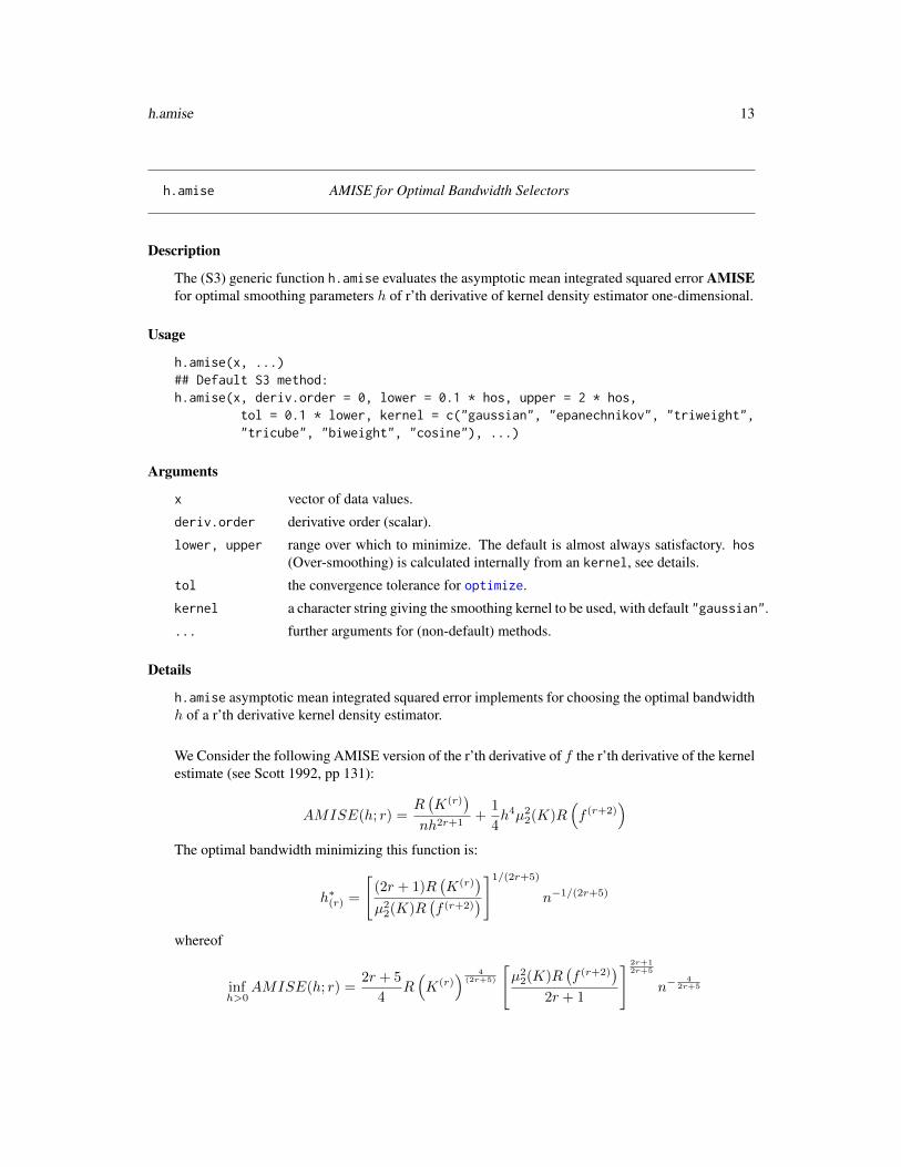
The (S3) generic function h.amise evaluates the asymptotic mean integrated squared error AMISEfor optimal smoothing parameters h of r’th derivative of kernel density estimator one-dimensional.

Usage

h.amise(x, ...)## Default S3 method:h.amise(x, deriv.order = 0, lower = 0.1 * hos, upper = 2 * hos,

tol = 0.1 * lower, kernel = c("gaussian", "epanechnikov", "triweight","tricube", "biweight", "cosine"), ...)

Arguments

x vector of data values.


lower, upper range over which to minimize. The default is almost always satisfactory. hos(Over-smoothing) is calculated internally from an kernel, see details.

tol the convergence tolerance for optimize.



Details

h.amise asymptotic mean integrated squared error implements for choosing the optimal bandwidthh of a r’th derivative kernel density estimator.

We Consider the following AMISE version of the r’th derivative of f the r’th derivative of the kernelestimate (see Scott 1992, pp 131):

AMISE(h; r) =R(K(r)

)nh2r+1

+1

4h4µ2

2(K)R(f (r+2)

)The optimal bandwidth minimizing this function is:

h∗(r) =

[(2r + 1)R

(K(r)

)µ22(K)R

(f (r+2)

)]1/(2r+5)

n−1/(2r+5)

whereof

infh>0

AMISE(h; r) =2r + 5

4R(K(r)

) 4(2r+5)

[µ22(K)R

(f (r+2)

)2r + 1

] 2r+12r+5

n−4

2r+5

14 h.amise

which is the smallest possible AMISE for estimation of f (r)(x) using the kernel K(x), whereR(K(r)

)=∫RK(r)(x)2dx and µ2(K) =

∫Rx2K(x)dx.

The range over which to minimize is hos Oversmoothing bandwidth, the default is almost alwayssatisfactory. See George and Scott (1985), George (1990), Scott (1992, pp 165), Wand and Jones(1995, pp 61).

Value




kernel name of kernel to use


h value of bandwidth parameter.

amise the AMISE value.

Author(s)


References







See Also

plot.h.amise, see nmise in package sm this function evaluates the mean integrated squared errorof a density estimate (deriv.order = 0) which is constructed from data which follow a normaldistribution.

Examples

## Derivative order = 0

h.amise(kurtotic,deriv.order = 0)


h.bcv 15


h.amise(kurtotic,deriv.order = 1)

h.bcv Biased Cross-Validation for Bandwidth Selection

Description

The (S3) generic function h.bcv computes the biased cross-validation bandwidth selector of r’thderivative of kernel density estimator one-dimensional.

Usage

h.bcv(x, ...)## Default S3 method:h.bcv(x, whichbcv = 1, deriv.order = 0, lower = 0.1 * hos, upper = 2 * hos,

tol = 0.1 * lower, kernel = c("gaussian","epanechnikov","triweight","tricube","biweight","cosine"), ...)

Arguments


whichbcv method selected, 1 = BCV1 or 2 = BCV2, see details.






Details

h.bcv biased cross-validation implements for choosing the bandwidth h of a r’th derivative ker-nel density estimator. if whichbcv = 1 then BCV1 is selected (Scott and George 1987), and ifwhichbcv = 2 used BCV2 (Jones and Kappenman 1991).

Scott and George (1987) suggest a method which has as its immediate target the AMISE (e.g.Silverman 1986, section 3.3). We denote θr(h) and θr(h) (Peter and Marron 1987, Jones andKappenman 1991) by:

θr(h) =(−1)r

n(n− 1)h2r+1

n∑i=1

n∑j=1;j 6=i

K(r) ∗K(r)

(Xj −Xi

h

)and

16 h.bcv

θr(h) =(−1)r

n(n− 1)h2r+1

n∑i=1

n∑j=1;j 6=i

K(2r)

(Xj −Xi

h

)

Scott and George (1987) proposed using θr(h) to estimate f (r)(x). Thus, h(r)BCV 1, say, is the h thatminimises:

BCV 1(h; r) =R(K(r)

)nh2r+1

+1

4µ22(K)h4θr+2(h)

and we define h(r)BCV 2 as the minimiser of (Jones and Kappenman 1991):

BCV 2(h; r) =R(K(r)

)nh2r+1

+1

4µ22(K)h4θr+2(h)

whereK(r)∗K(r)(x) is the convolution of the r’th derivative kernel functionK(r)(x) (see kernel.convand kernel.fun); R

(K(r)


∫Rx2K(x)dx.


Value






whichbcv method selected.


min.bcv the minimal BCV value.

Author(s)


References





h.ccv 17

Sheather,S. J. (2004). Density estimation. Statistical Science, 19, 588–597.




See Also

plot.h.bcv, see bw.bcv in package "stats" and bcv in package MASS for Gaussian kernel only ifderiv.order = 0, Hbcv for bivariate data in package ks for Gaussian kernel only if deriv.order = 0,kdeb in package locfit if deriv.order = 0.

Examples

## EXAMPLE 1:

x <- rnorm(100)h.bcv(x,whichbcv = 1, deriv.order = 0)h.bcv(x,whichbcv = 2, deriv.order = 0)

## EXAMPLE 2:


h.bcv(kurtotic,deriv.order = 0)


h.bcv(kurtotic,deriv.order = 1)

h.ccv Complete Cross-Validation for Bandwidth Selection

Description

The (S3) generic function h.ccv computes the complete cross-validation bandwidth selector of r’thderivative of kernel density estimator one-dimensional.

Usage

h.ccv(x, ...)## Default S3 method:h.ccv(x, deriv.order = 0, lower = 0.1 * hos, upper = hos,

tol = 0.1 * lower, kernel = c("gaussian", "triweight","tricube", "biweight", "cosine"), ...)


http://CRAN.R-project.org/package=MASS



18 h.ccv

Arguments

x vector of data values.deriv.order derivative order (scalar).lower, upper range over which to minimize. The default is almost always satisfactory. hos

(Over-smoothing) is calculated internally from an kernel, see details.tol the convergence tolerance for optimize.kernel a character string giving the smoothing kernel to be used, with default "gaussian".... further arguments for (non-default) methods.

Details

h.ccv complete cross-validation implements for choosing the bandwidth h of a r’th derivative ker-nel density estimator.

Jones and Kappenman (1991) proposed a so-called complete cross-validation (CCV) in kernel den-sity estimator. This method can be extended to the estimation of derivative of the density, basingour estimate of integrated squared density derivative (Peter and Marron 1987) on the θr(h)’s, weget the following, start from R

(f(r)h

)− θr(h) as an estimate of MISE. Thus, h(r)CCV , say, is the h

that minimises:

CCV (h; r) = R(f(r)h

)− θr(h) +

1

2µ2(K)h2θr+1(h) +

1

24

(6µ2

2(K)− δ(K))h4θr+2(h)

with

R(f(r)h

)=

∫ (f(r)h (x)

)2dx =

R(K(r)

)nh2r+1

+(−1)r

n(n− 1)h2r+1

n∑i=1

n∑j=1;j 6=i

K(r)∗K(r)

(Xj −Xi

h

)and

θr(h) =(−1)r

n(n− 1)h2r+1

n∑i=1

n∑j=1;j 6=i

K(2r)

(Xj −Xi

h

)andK(r)∗K(r)(x) is the convolution of the r’th derivative kernel functionK(r)(x) (see kernel.convand kernel.fun);R

(K(r)


∫Rx2K(x)dx, δ(K) =

∫Rx4K(x)dx.


Value

x data points - same as input.data.name the deparsed name of the x argument.n the sample size after elimination of missing values.kernel name of kernel to usederiv.order the derivative order to use.h value of bandwidth parameter.min.ccv the minimal CCV value.

h.mcv 19

Author(s)


References



See Also

plot.h.ccv.

Examples


h.ccv(kurtotic,deriv.order = 0)


h.ccv(kurtotic,deriv.order = 1)

h.mcv Modified Cross-Validation for Bandwidth Selection

Description

The (S3) generic function h.mcv computes the modified cross-validation bandwidth selector of r’thderivative of kernel density estimator one-dimensional.

Usage

h.mcv(x, ...)## Default S3 method:h.mcv(x, deriv.order = 0, lower = 0.1 * hos, upper = 2 * hos,

tol = 0.1 * lower, kernel = c("gaussian", "epanechnikov", "triweight","tricube", "biweight", "cosine"), ...)

Arguments





20 h.mcv



Details

h.mcv modified cross-validation implements for choosing the bandwidth h of a r’th derivative ker-nel density estimator.

Stute (1992) proposed a so-called modified cross-validation (MCV) in kernel density estimator.This method can be extended to the estimation of derivative of a density, the essential idea basedon approximated the problematic term by the aid of the Hajek projection (see Stute 1992). Theminimization criterion is defined by:

MCV (h; r) =R(K(r)

)nh2r+1

+(−1)r

n(n− 1)h2r+1

n∑i=1

n∑j=1;j 6=i

ϕ(r)

(Xj −Xi

h

)whit

ϕ(r)(c) =

(K(r) ∗K(r) −K(2r) − µ2(K)

2K(2r+2)

)(c)

andK(r)∗K(r)(x) is the convolution of the r’th derivative kernel functionK(r)(x) (see kernel.convand kernel.fun); R

(K(r)


∫Rx2K(x)dx.


Value







min.mcv the minimal MCV value.

Author(s)


References

Heidenreich, N. B., Schindler, A. and Sperlich, S. (2013). Bandwidth selection for kernel densityestimation: a review of fully automatic selectors. Advances in Statistical Analysis.

Stute, W. (1992). Modified cross validation in density estimation. Journal of Statistical Planningand Inference, 30, 293–305.

h.mlcv 21

See Also

plot.h.mcv.

Examples


h.mcv(kurtotic,deriv.order = 0)


h.mcv(kurtotic,deriv.order = 1)

h.mlcv Maximum-Likelihood Cross-validation for Bandwidth Selection

Description

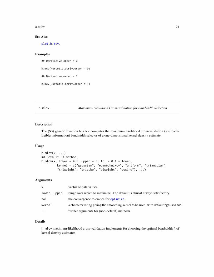
The (S3) generic function h.mlcv computes the maximum likelihood cross-validation (Kullback-Leibler information) bandwidth selector of a one-dimensional kernel density estimate.

Usage

h.mlcv(x, ...)## Default S3 method:h.mlcv(x, lower = 0.1, upper = 5, tol = 0.1 * lower,

kernel = c("gaussian", "epanechnikov", "uniform", "triangular","triweight", "tricube", "biweight", "cosine"), ...)

Arguments


lower, upper range over which to maximize. The default is almost always satisfactory.




Details

h.mlcv maximum-likelihood cross-validation implements for choosing the optimal bandwidth h ofkernel density estimator.

22 h.mlcv

This method was proposed by Habbema, Hermans, and Van den Broeck (1971) and by Duin (1976).The maximum-likelihood cross-validation (MLCV) function is defined by:

MLCV (h) = n−1n∑i=1

log[fh,i(x)

]the estimate fh,i(x) on the subset {Xj}j 6=i denoting the leave-one-out estimator, can be written:

fh,i(Xi) =1

(n− 1)h

∑j 6=i

K

(Xj −Xi

h

)

Define that hmlcv as good which approaches the finite maximum of MLCV (h):

hmlcv = arg maxh

MLCV (h) = arg maxh

n−1 n∑i=1

log

∑j 6=i

K

(Xj −Xi

h

)− log[(n− 1)h]

Value






mlcv the maximal likelihood CV value.

Author(s)


References

Habbema, J. D. F., Hermans, J., and Van den Broek, K. (1974) A stepwise discrimination analy-sis program using density estimation. Compstat 1974: Proceedings in Computational Statistics.Physica Verlag, Vienna.

Duin, R. P. W. (1976). On the choice of smoothing parameters of Parzen estimators of probabilitydensity functions. IEEE Transactions on Computers, C-25, 1175–1179.

See Also

plot.h.mlcv, see lcv in package locfit.

Examples

h.mlcv(bimodal)h.mlcv(bimodal, kernel ="epanechnikov")


h.tcv 23

h.tcv Trimmed Cross-Validation for Bandwidth Selection

Description

The (S3) generic function h.tcv computes the trimmed cross-validation bandwidth selector of r’thderivative of kernel density estimator one-dimensional.

Usage

h.tcv(x, ...)## Default S3 method:h.tcv(x, deriv.order = 0, lower = 0.1 * hos, upper = 2 * hos,

tol = 0.1 * lower, kernel = c("gaussian", "epanechnikov", "uniform","triangular", "triweight", "tricube", "biweight", "cosine"), ...)

Arguments







Details

h.tcv trimmed cross-validation implements for choosing the bandwidth h of a r’th derivative kerneldensity estimator.

Feluch and Koronacki (1992) proposed a so-called trimmed cross-validation (TCV) in kernel den-sity estimator, a simple modification of the unbiased (least-squares) cross-validation criterion. Weconsider the following "trimmed" version of "unbiased", to be minimized with respect to h:∫ (

f(r)h (x)

)2− 2

(−1)r

n(n− 1)h2r+1

n∑i=1

∑j=1;j 6=i

K(2r)

(Xj −Xi

h

)χ (|Xi −Xj | > cn)

where χ(.) denotes the indicator function and cn is a sequence of positive constants, cn/h2r+1 → 0as n→∞, and∫ (

f(r)h (x)

)2=R(K(r)

)nh2r+1

+(−1)r

n(n− 1)h2r+1

n∑i=1

n∑j=1;j 6=i

K(r) ∗K(r)

(Xj −Xi

h

)

24 h.tcv

the trimmed cross-validation function is defined by:

TCV (h; r) =R(K(r)

)nh2r+1

+(−1)r

n(n− 1)h2r+1

n∑i=1

n∑j=1;j 6=i

ϕ(r)

(Xj −Xi

h

)whit

ϕ(r)(c) =(K(r) ∗K(r) − 2K(2r)χ

(|c| > cn/h

2r+1))

(c)

here we take cn = 1/n, for assure the convergence. Where K(r) ∗ K(r)(x) is the convolution ofthe r’th derivative kernel function K(r)(x) (see kernel.conv and kernel.fun).


Value







min.tcv the minimal TCV value.

Author(s)


References

Feluch, W. and Koronacki, J. (1992). A note on modified cross-validation in density estimation.Computational Statistics and Data Analysis, 13, 143–151.

See Also

plot.h.tcv.

Examples


h.tcv(kurtotic,deriv.order = 0)


h.tcv(kurtotic,deriv.order = 1)

h.ucv 25

h.ucv Unbiased (Least-Squares) Cross-Validation for Bandwidth Selection

Description

The (S3) generic function h.ucv computes the unbiased (least-squares) cross-validation bandwidthselector of r’th derivative of kernel density estimator one-dimensional.

Usage

h.ucv(x, ...)## Default S3 method:h.ucv(x, deriv.order = 0, lower = 0.1 * hos, upper = 2 * hos,

tol = 0.1 * lower, kernel = c("gaussian", "epanechnikov", "uniform","triangular", "triweight", "tricube", "biweight", "cosine"), ...)

Arguments







Details

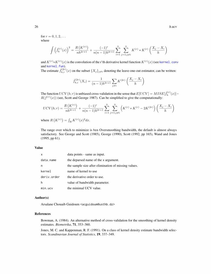
h.ucv unbiased (least-squares) cross-validation implements for choosing the bandwidth h of a r’thderivative kernel density estimator.

Rudemo (1982) and Bowman (1984) proposed a so-called unbiased (least-squares) cross-validation(UCV) in kernel density estimator. An adaptation of unbiased cross-validation is proposed by Wolf-gang et al. (1990) for bandwidth choice in the r’th derivative of kernel density estimator. The essen-tial idea of this methods, for the estimation of f (r)(x) (r is derivative order), is to use the bandwidthh which minimizes the function:

UCV (h; r) =

∫ (f(r)h (x)

)2− 2n−1(−1)r

n∑i=1

f(2r)h,i (Xi)

The bandwidth minimizing this function is:

h(r)ucv = arg minh(r)

UCV (h; r)

26 h.ucv

for r = 0, 1, 2, . . .where ∫ (

f(r)h (x)

)2=R(K(r)

)nh2r+1

+(−1)r

n(n− 1)h2r+1

n∑i=1

n∑j=1;j 6=i

K(r) ∗K(r)

(Xj −Xi

h

)

andK(r)∗K(r)(x) is the convolution of the r’th derivative kernel functionK(r)(x) (see kernel.convand kernel.fun).The estimate f (2r)h,i (x) on the subset {Xj}j 6=i denoting the leave-one-out estimator, can be written:

f(2r)h,i (Xi) =

1

(n− 1)h2r+1

∑j 6=i

K(2r)

(Xj −Xi

h

)

The functionUCV (h; r) is unbiased cross-validation in the sense thatE[UCV ] = MISE[f(r)h (x)]−

R(f (r)(x)) (see, Scott and George 1987). Can be simplified to give the computationally:

UCV (h; r) =R(K(r)

)nh2r+1

+(−1)r

n(n− 1)h2r+1

n∑i=1

n∑j=1;j 6=i

(K(r) ∗K(r) − 2K(2r)

)(Xj −Xi

h

)

where R(K(r)

)=∫RK(r)(x)2dx.


Value







min.ucv the minimal UCV value.

Author(s)


References

Bowman, A. (1984). An alternative method of cross-validation for the smoothing of kernel densityestimates. Biometrika, 71, 353–360.


kernel.conv 27



Rudemo, M. (1982). Empirical choice of histograms and kernel density estimators. ScandinavianJournal of Statistics, 9, 65–78.






Wolfgang, H., Marron, J. S. and Wand, M. P. (1990). Bandwidth choice for density derivatives.Journal of the Royal Statistical Society, Series B, 223–232.

See Also

plot.h.ucv, see bw.ucv in package "stats" and ucv in package MASS for Gaussian kernel only ifderiv.order = 0, hlscv in package ks for Gaussian kernel only if 0 <= deriv.order <= 5,kdeb in package locfit if deriv.order = 0.

Examples


h.ucv(kurtotic,deriv.order = 0)


h.ucv(kurtotic,deriv.order = 1)

kernel.conv Convolutions of r’th Derivative for Kernel Function

Description

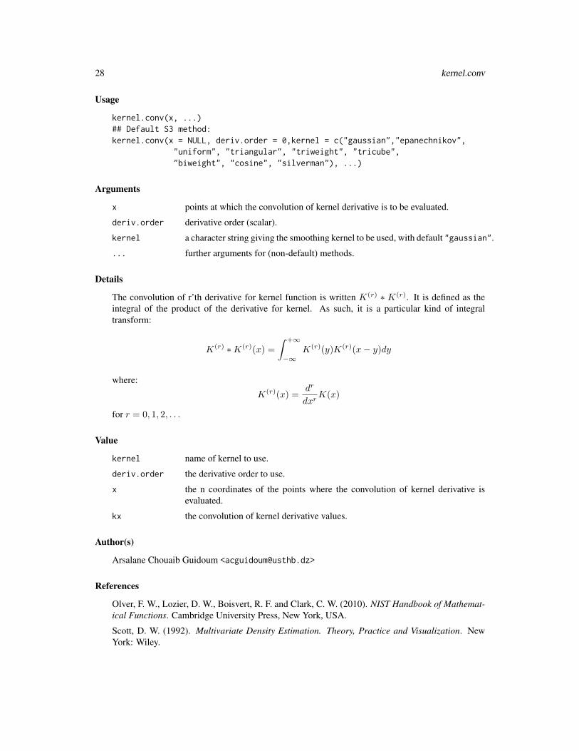
The (S3) generic function kernel.conv computes the convolution of r’th derivative for kernel func-tion.


http://CRAN.R-project.org/package=MASS



28 kernel.conv

Usage

kernel.conv(x, ...)## Default S3 method:kernel.conv(x = NULL, deriv.order = 0,kernel = c("gaussian","epanechnikov",

"uniform", "triangular", "triweight", "tricube","biweight", "cosine", "silverman"), ...)

Arguments

x points at which the convolution of kernel derivative is to be evaluated.




Details

The convolution of r’th derivative for kernel function is written K(r) ∗ K(r). It is defined as theintegral of the product of the derivative for kernel. As such, it is a particular kind of integraltransform:

K(r) ∗K(r)(x) =

∫ +∞

−∞K(r)(y)K(r)(x− y)dy

where:

K(r)(x) =dr

dxrK(x)

for r = 0, 1, 2, . . .

Value



x the n coordinates of the points where the convolution of kernel derivative isevaluated.

kx the convolution of kernel derivative values.

Author(s)


References



kernel.fun 29




See Also

plot.kernel.conv, kernapply in package "stats" for computes the convolution between an inputsequence, and convolve use the Fast Fourier Transform (fft) to compute the several kinds ofconvolutions of two sequences.

Examples

kernels <- eval(formals(kernel.conv.default)$kernel)kernels

## gaussiankernel.conv(x = 0,kernel=kernels[1],deriv.order=0)kernel.conv(x = 0,kernel=kernels[1],deriv.order=1)

## silvermankernel.conv(x = 0,kernel=kernels[9],deriv.order=0)kernel.conv(x = 0,kernel=kernels[9],deriv.order=1)

kernel.fun Derivatives of Kernel Function

Description

The (S3) generic function kernel.fun computes the r’th derivative for kernel density.

Usage

kernel.fun(x, ...)## Default S3 method:kernel.fun(x = NULL, deriv.order = 0, kernel = c("gaussian","epanechnikov",

"uniform", "triangular", "triweight", "tricube","biweight", "cosine", "silverman"), ...)

Arguments

x points at which the derivative of kernel function is to be evaluated.




30 kernel.fun

Details

We give a short survey of some kernels functions K(x; r); where r is derivative order,

• Gaussian: K(x;∞) = 1√2π

exp(−x

2

2

)1]−∞,+∞[

• Epanechnikov: K(x; 2) = 34 (1− x2)1(|x|≤1)

• uniform (rectangular): K(x; 0) = 121(|x|≤1)

• triangular: K(x; 1) = (1− |x|)1(|x|≤1)• triweight: K(x; 6) = 35

32 (1− x2)31(|x|≤1)

• tricube: K(x; 9) = 7081 (1− |x|3)31(|x|≤1)

• biweight: K(x; 4) = 1516 (1− x2)21(|x|≤1)

• cosine: K(x;∞) = π4 cos

(π2x)

1(|x|≤1)

• Silverman: K(x; r%%8)1 = 12 exp

(− |x|√

2

)sin(|x|√2

+ π4

)1]−∞,+∞[

The r’th derivative for kernel function K(x) is written:

K(r)(x) =dr

dxrK(x)

for r = 0, 1, 2, . . .The r’th derivative of the Gaussian kernel K(x) is given by:

K(r)(x) = (−1)rHr(x)K(x)

where Hr(x) is the r’th Hermite polynomial. This polynomials are set of orthogonal polynomials,for more details see, hermite.h.polynomials in package orthopolynom.

Value



x the n coordinates of the points where the derivative of kernel function is evalu-ated.

kx the kernel derivative values.

Author(s)


References

Jones, M. C. (1992). Differences and derivatives in kernel estimation. Metrika, 39, 335–340.



1%% indicates x mod y

http://CRAN.R-project.org/package=orthopolynom

plot.dkde 31

See Also

plot.kernel.fun, deriv and D in package "stats" for symbolic and algorithmic derivatives ofsimple expressions.

Examples

kernels <- eval(formals(kernel.fun.default)$kernel)kernels

## gaussiankernel.fun(x = 0,kernel=kernels[1],deriv.order=0)kernel.fun(x = 0,kernel=kernels[1],deriv.order=1)

## silvermankernel.fun(x = 0,kernel=kernels[9],deriv.order=0)kernel.fun(x = 0,kernel=kernels[9],deriv.order=1)

plot.dkde Plot for Kernel Density Derivative Estimate

Description

The plot.dkde function loops through calls to the dkde function. Plot for kernel density derivativeestimate for 1-dimensional data.

Usage

## S3 method for class 'dkde'plot(x, fx = NULL, ...)## S3 method for class 'dkde'lines(x, ...)

Arguments

x object of class dkde (output from dkde).

fx add to graphics the true density derivative (class :function), to compare it bythe density derivative to estimate.

... other graphics parameters, see par in package "graphics".

Details

The 1-d plot is a standard plot of a 1-d curve. If !is.null(fx) then a true density derivative isadded.

Value

Plot of 1-d kernel density derivative estimates are sent to graphics window.

32 plot.h.amise

Author(s)


See Also

dkde, plot.density in package "stats" if deriv.order = 0.

Examples

plot(dkde(kurtotic,deriv.order=0,kernel="gaussian"),sub="")lines(dkde(kurtotic,deriv.order=0,kernel="biweight"),col="red")

plot.h.amise Plot for Asymptotic Mean Integrated Squared Error

Description

The plot.h.amise function loops through calls to the h.amise function. Plot for asymptotic meanintegrated squared error function for 1-dimensional data.

Usage

## S3 method for class 'h.amise'plot(x, seq.bws=NULL, ...)## S3 method for class 'h.amise'lines(x,seq.bws=NULL, ...)

Arguments

x object of class h.amise (output from h.amise).

seq.bws the sequence of bandwidths in which to compute the AMISE function. By de-fault, the procedure defines a sequence of 50 points, from 0.15*hos to 2*hos(Over-smoothing).


Value

Plot of 1-d AMISE function are sent to graphics window.



seq.bws the sequence of bandwidths.

amise the values of the AMISE function in the bandwidths grid.

plot.h.bcv 33

Author(s)


See Also

h.amise.

Examples

plot(h.amise(bimodal,deriv.order=0))

plot.h.bcv Plot for Biased Cross-Validation

Description

The plot.h.bcv function loops through calls to the h.bcv function. Plot for biased cross-validationfunction for 1-dimensional data.

Usage

## S3 method for class 'h.bcv'plot(x, seq.bws=NULL, ...)## S3 method for class 'h.bcv'lines(x,seq.bws=NULL, ...)

Arguments

x object of class h.bcv (output from h.bcv).

seq.bws the sequence of bandwidths in which to compute the biased cross-validationfunction. By default, the procedure defines a sequence of 50 points, from 0.15*hosto 2*hos (Over-smoothing).


Value

Plot of 1-d biased cross-validation function are sent to graphics window.




bcv the values of the biased cross-validation function in the bandwidths grid.

Author(s)


34 plot.h.ccv

See Also

h.bcv.

Examples

## EXAMPLE 1:

plot(h.bcv(trimodal, whichbcv = 1, deriv.order = 0),main="",sub="")lines(h.bcv(trimodal, whichbcv = 2, deriv.order = 0),col="red")legend("topright", c("BCV1","BCV2"),lty=1,col=c("black","red"),inset = .015)

## EXAMPLE 2:

plot(h.bcv(trimodal, whichbcv = 1, deriv.order = 1),main="",sub="")lines(h.bcv(trimodal, whichbcv = 2, deriv.order = 1),col="red")legend("topright", c("BCV1","BCV2"),lty=1,col=c("black","red"),inset = .015)

plot.h.ccv Plot for Complete Cross-Validation

Description

The plot.h.ccv function loops through calls to the h.ccv function. Plot for complete cross-validation function for 1-dimensional data.

Usage

## S3 method for class 'h.ccv'plot(x, seq.bws=NULL, ...)## S3 method for class 'h.ccv'lines(x,seq.bws=NULL, ...)

Arguments

x object of class h.ccv (output from h.ccv).seq.bws the sequence of bandwidths in which to compute the complete cross-validation

function. By default, the procedure defines a sequence of 50 points, from 0.15*hosto 2*hos (Over-smoothing).


Value

Plot of 1-d complete cross-validation function are sent to graphics window.

kernel name of kernel to use.deriv.order the derivative order to use.seq.bws the sequence of bandwidths.ccv the values of the complete cross-validation function in the bandwidths grid.

plot.h.mcv 35

Author(s)


See Also

h.ccv.

Examples

par(mfrow=c(2,1))plot(h.ccv(trimodal,deriv.order=0),main="")plot(h.ccv(trimodal,deriv.order=1),main="")

plot.h.mcv Plot for Modified Cross-Validation

Description

The plot.h.mcv function loops through calls to the h.mcv function. Plot for modified cross-validation function for 1-dimensional data.

Usage

## S3 method for class 'h.mcv'plot(x, seq.bws=NULL, ...)## S3 method for class 'h.mcv'lines(x,seq.bws=NULL, ...)

Arguments

x object of class h.mcv (output from h.mcv).

seq.bws the sequence of bandwidths in which to compute the modified cross-validationfunction. By default, the procedure defines a sequence of 50 points, from 0.15*hosto 2*hos (Over-smoothing).


Value

Plot of 1-d modified cross-validation function are sent to graphics window.




mcv the values of the modified cross-validation function in the bandwidths grid.

36 plot.h.mlcv

Author(s)


See Also

h.mcv.

Examples

par(mfrow=c(2,1))plot(h.mcv(trimodal,deriv.order=0),main="")plot(h.mcv(trimodal,deriv.order=1),main="")

plot.h.mlcv Plot for Maximum-Likelihood Cross-validation

Description

The plot.h.mlcv function loops through calls to the h.mlcv function. Plot for maximum-likelihoodcross-validation function for 1-dimensional data.

Usage

## S3 method for class 'h.mlcv'plot(x, seq.bws=NULL, ...)## S3 method for class 'h.mlcv'lines(x,seq.bws=NULL, ...)

Arguments

x object of class h.mlcv (output from h.mlcv).

seq.bws the sequence of bandwidths in which to compute the maximum- likelihoodcross-validation function. By default, the procedure defines a sequence of 50points, from 0.15*hos to 2*hos (Over-smoothing).


Value

Plot of 1-d maximum-likelihood cross-validation function are sent to graphics window.



mlcv the values of the maximum-likelihood cross-validation function in the band-widths grid.

plot.h.tcv 37

Author(s)


See Also

h.mlcv.

Examples

plot(h.mlcv(bimodal))

plot.h.tcv Plot for Trimmed Cross-Validation

Description

The plot.h.tcv function loops through calls to the h.tcv function. Plot for trimmed cross-validation function for 1-dimensional data.

Usage

## S3 method for class 'h.tcv'plot(x, seq.bws=NULL, ...)## S3 method for class 'h.tcv'lines(x,seq.bws=NULL, ...)

Arguments

x object of class h.tcv (output from h.tcv).

seq.bws the sequence of bandwidths in which to compute the trimmed cross-validationfunction. By default, the procedure defines a sequence of 50 points, from 0.15*hosto 2*hos (Over-smoothing).


Value

Plot of 1-d trimmed cross-validation function are sent to graphics window.




tcv the values of the trimmed cross-validation function in the bandwidths grid.

Author(s)


38 plot.h.ucv

See Also

h.tcv.

Examples

par(mfrow=c(2,1))plot(h.tcv(trimodal,deriv.order=0),main="")plot(h.tcv(trimodal,deriv.order=1),seq.bws=seq(0.1,0.5,length.out=50),main="")

plot.h.ucv Plot for Unbiased Cross-Validation

Description

The plot.h.ucv function loops through calls to the h.ucv function. Plot for unbiased cross-validation function for 1-dimensional data.

Usage

## S3 method for class 'h.ucv'plot(x, seq.bws=NULL, ...)## S3 method for class 'h.ucv'lines(x,seq.bws=NULL, ...)

Arguments

x object of class h.ucv (output from h.ucv).

seq.bws the sequence of bandwidths in which to compute the unbiased cross-validationfunction. By default, the procedure defines a sequence of 50 points, from 0.15*hosto 2*hos (Over-smoothing).


Value

Plot of 1-d unbiased cross-validation function are sent to graphics window.




ucv the values of the unbiased cross-validation function in the bandwidths grid.

Author(s)


plot.kernel.conv 39

See Also

h.ucv.

Examples

par(mfrow=c(2,1))plot(h.ucv(trimodal,deriv.order=0),seq.bws=seq(0.06,0.2,length=50))plot(h.ucv(trimodal,deriv.order=1),seq.bws=seq(0.06,0.2,length=50))

plot.kernel.conv Plot for Convolutions of r’th Derivative Kernel Function

Description

The plot.kernel.conv function loops through calls to the kernel.conv function. Plot for convo-lutions of r’th derivative kernel function one-dimensional.

Usage

## S3 method for class 'kernel.conv'plot(x, ...)

Arguments

x object of class kernel.conv (output from kernel.conv).


Value

Plot of 1-d for convolution of r’th derivative kernel function are sent to graphics window.

Author(s)


See Also

kernel.conv.

Examples

## Gaussian kernel

dev.new()par(mfrow=c(2,2))plot(kernel.conv(kernel="gaussian",deriv.order=0))plot(kernel.conv(kernel="gaussian",deriv.order=1))plot(kernel.conv(kernel="gaussian",deriv.order=2))

40 plot.kernel.fun

plot(kernel.conv(kernel="gaussian",deriv.order=3))

## Silverman kernel

dev.new()par(mfrow=c(2,2))plot(kernel.conv(kernel="silverman",deriv.order=0))plot(kernel.conv(kernel="silverman",deriv.order=1))plot(kernel.conv(kernel="silverman",deriv.order=2))plot(kernel.conv(kernel="silverman",deriv.order=3))

plot.kernel.fun Plot of r’th Derivative Kernel Function

Description

The plot.kernel.fun function loops through calls to the kernel.fun function. Plot for r’thderivative kernel function one-dimensional.

Usage

## S3 method for class 'kernel.fun'plot(x, ...)

Arguments

x object of class kernel.fun (output from kernel.fun).


Value

Plot of 1-d for r’th derivative kernel function are sent to graphics window.

Author(s)


See Also

kernel.fun.

Examples

## Gaussian kernel

dev.new()par(mfrow=c(2,2))plot(kernel.fun(kernel="gaussian",deriv.order=0))plot(kernel.fun(kernel="gaussian",deriv.order=1))

plot.kernel.fun 41

plot(kernel.fun(kernel="gaussian",deriv.order=2))plot(kernel.fun(kernel="gaussian",deriv.order=3))

## Silverman kernel

dev.new()par(mfrow=c(2,2))plot(kernel.fun(kernel="silverman",deriv.order=0))plot(kernel.fun(kernel="silverman",deriv.order=1))plot(kernel.fun(kernel="silverman",deriv.order=2))plot(kernel.fun(kernel="silverman",deriv.order=3))

Index

∗Topic bandwidth selectionh.amise, 13h.bcv, 15h.ccv, 17h.mcv, 19h.mlcv, 21h.tcv, 23h.ucv, 25

∗Topic datasetsClaw, Bimodal, Kurtotic, Outlier,

Trimodal, 7∗Topic density derivative

dkde, 9∗Topic kernel

kernel.conv, 27kernel.fun, 29

∗Topic nonparametricdkde, 9h.amise, 13h.bcv, 15h.ccv, 17h.mcv, 19h.mlcv, 21h.tcv, 23h.ucv, 25kernel.conv, 27kernel.fun, 29

∗Topic packagekedd-package, 2

∗Topic plotplot.dkde, 31plot.h.amise, 32plot.h.bcv, 33plot.h.ccv, 34plot.h.mcv, 35plot.h.mlcv, 36plot.h.tcv, 37plot.h.ucv, 38plot.kernel.conv, 39

plot.kernel.fun, 40∗Topic smooth

dkde, 9h.amise, 13h.bcv, 15h.ccv, 17h.mcv, 19h.mlcv, 21h.tcv, 23h.ucv, 25

bcv, 17bimodal (Claw, Bimodal, Kurtotic,

Outlier, Trimodal), 7bw.bcv, 17bw.ucv, 27

claw (Claw, Bimodal, Kurtotic,Outlier, Trimodal), 7

Claw, Bimodal, Kurtotic, Outlier,Trimodal, 7

convolve, 29

D, 31density, 12deriv, 31dkde, 3, 9, 31, 32

fft, 29function, 31

h.amise, 4, 13, 32, 33h.bcv, 4, 9, 15, 33, 34h.ccv, 4, 17, 34, 35h.mcv, 4, 19, 35, 36h.mlcv, 4, 21, 36, 37h.tcv, 4, 23, 37, 38h.ucv, 4, 9, 10, 25, 38, 39Hbcv, 17hermite.h.polynomials, 30hlscv, 27

42

INDEX 43

kdde, 12kdeb, 17, 27kedd (kedd-package), 2kedd-package, 2kernapply, 29kernel.conv, 3, 16, 18, 20, 24, 26, 27, 39kernel.fun, 3, 16, 18, 20, 24, 26, 29, 40kurtotic (Claw, Bimodal, Kurtotic,

Outlier, Trimodal), 7

lcv, 22lines.dkde, 3lines.dkde (plot.dkde), 31lines.h.amise, 4lines.h.amise (plot.h.amise), 32lines.h.bcv, 4lines.h.bcv (plot.h.bcv), 33lines.h.ccv, 4lines.h.ccv (plot.h.ccv), 34lines.h.mcv, 4lines.h.mcv (plot.h.mcv), 35lines.h.mlcv, 4lines.h.mlcv (plot.h.mlcv), 36lines.h.tcv, 4lines.h.tcv (plot.h.tcv), 37lines.h.ucv, 4lines.h.ucv (plot.h.ucv), 38

nmise, 14

optimize, 13, 15, 18, 19, 21, 23, 25outlier (Claw, Bimodal, Kurtotic,

Outlier, Trimodal), 7

par, 31–40plot.density, 32plot.dkde, 3, 12, 31, 31plot.h.amise, 4, 14, 32, 32plot.h.bcv, 4, 17, 33, 33plot.h.ccv, 4, 19, 34, 34plot.h.mcv, 4, 21, 35, 35plot.h.mlcv, 4, 22, 36, 36plot.h.tcv, 4, 24, 37, 37plot.h.ucv, 4, 27, 38, 38plot.kernel.conv, 29, 39, 39plot.kernel.fun, 31, 40, 40print.dkde (dkde), 9print.h.amise (h.amise), 13print.h.bcv (h.bcv), 15

print.h.ccv (h.ccv), 17print.h.mcv (h.mcv), 19print.h.mlcv (h.mlcv), 21print.h.tcv (h.tcv), 23print.h.ucv (h.ucv), 25

rnorMix, 8

trimodal (Claw, Bimodal, Kurtotic,Outlier, Trimodal), 7

ucv, 27

Package ‘kedd’ - R · Maintainer Arsalane Chouaib Guidoum Depends R (>= 2.15.0) Description...

Documents

Transcript of Package ‘kedd’ - R · Maintainer Arsalane Chouaib Guidoum Depends R (>= 2.15.0) Description...