Package ‘hamlet’ - R · The package ’hamlet’ offers functions for optimal matching,...

Package ‘hamlet’May 27, 2018

Type Package

Title Hierarchical Optimal Matching and Machine Learning Toolbox

Version 0.9.6

Date 2018-05-26

Author Teemu Daniel Laajala <[email protected]>

Maintainer Teemu Daniel Laajala <[email protected]>

Depends R (>= 3.0.0)

Imports grDevices, graphics, stats, utils

Suggests lme4, nlme, amap, nbpMatching, lattice, lmerTest, xtable,Cairo, Matrix, MASS

Description Various functions and algorithms are provided here for solving optimal match-ing tasks in the context of preclinical cancer studies. Further, various helper and plotting func-tions are provided for unsupervised and supervised machine learning as well as longitudi-nal mixed-effects modeling of tumor growth response patterns.

License GPL (>= 2)

NeedsCompilation no

Repository CRAN

Date/Publication 2018-05-26 22:01:24 UTC

R topics documented:hamlet-package . . . . . . . . . . . . . . . . . . . . . . . . . . . . . . . . . . . . . . . 2extendsymrange . . . . . . . . . . . . . . . . . . . . . . . . . . . . . . . . . . . . . . . 4hmap . . . . . . . . . . . . . . . . . . . . . . . . . . . . . . . . . . . . . . . . . . . . 5hmap.annotate . . . . . . . . . . . . . . . . . . . . . . . . . . . . . . . . . . . . . . . . 8hmap.key . . . . . . . . . . . . . . . . . . . . . . . . . . . . . . . . . . . . . . . . . . 10match.allocate . . . . . . . . . . . . . . . . . . . . . . . . . . . . . . . . . . . . . . . . 12match.bb . . . . . . . . . . . . . . . . . . . . . . . . . . . . . . . . . . . . . . . . . . . 13match.dummy . . . . . . . . . . . . . . . . . . . . . . . . . . . . . . . . . . . . . . . . 15match.ga . . . . . . . . . . . . . . . . . . . . . . . . . . . . . . . . . . . . . . . . . . . 16match.mat2vec . . . . . . . . . . . . . . . . . . . . . . . . . . . . . . . . . . . . . . . 19

1

2 hamlet-package

match.vec2mat . . . . . . . . . . . . . . . . . . . . . . . . . . . . . . . . . . . . . . . 21mem.getcomp . . . . . . . . . . . . . . . . . . . . . . . . . . . . . . . . . . . . . . . . 22mem.plotran . . . . . . . . . . . . . . . . . . . . . . . . . . . . . . . . . . . . . . . . . 23mem.plotresid . . . . . . . . . . . . . . . . . . . . . . . . . . . . . . . . . . . . . . . . 24mem.powersimu . . . . . . . . . . . . . . . . . . . . . . . . . . . . . . . . . . . . . . . 25mix.binary . . . . . . . . . . . . . . . . . . . . . . . . . . . . . . . . . . . . . . . . . . 27mix.fun . . . . . . . . . . . . . . . . . . . . . . . . . . . . . . . . . . . . . . . . . . . 28mixplot . . . . . . . . . . . . . . . . . . . . . . . . . . . . . . . . . . . . . . . . . . . 29orxlong . . . . . . . . . . . . . . . . . . . . . . . . . . . . . . . . . . . . . . . . . . . 31orxwide . . . . . . . . . . . . . . . . . . . . . . . . . . . . . . . . . . . . . . . . . . . 33smartjitter . . . . . . . . . . . . . . . . . . . . . . . . . . . . . . . . . . . . . . . . . . 34vcaplong . . . . . . . . . . . . . . . . . . . . . . . . . . . . . . . . . . . . . . . . . . . 35vcapwide . . . . . . . . . . . . . . . . . . . . . . . . . . . . . . . . . . . . . . . . . . 37

Index 40

hamlet-package Hierarchical Optimal Matching and Machine Learning Toolbox

Description

This package provides functions and algorithms for solving optimal matching tasks in the contextof preclinical cancer studies. Further, various help and plotting functions are provided for unsuper-vised and supervised machine learning as well as longitudinal modeling of tumor growth responsepatterns.

Details

Package: hamletType: PackageVersion: 0.9.5-2Date: 2017-09-21License: GPL (>= 2)

The package ’hamlet’ offers functions for optimal matching, randomization, and mixed-effectsmodeling in preclinical cancer studies. The functions are divided to ’match’-prefix indicating opti-mal matching intended functions, ’mem’ indicating mixed-effects modeling, ’mix’ for mixed type(numerical and categorical) data analysis, and rest that are various plotting and helper functions forvarious tasks.

Author(s)

Teemu Daniel Laajala

Maintainer: Teemu Daniel Laajala <[email protected]>

hamlet-package 3

References

Laajala TD, Jumppanen M, Huhtaniemi R, Fey V, Kaur A, et al. (2016) Optimized design and analy-sis of preclinical intervention studies in vivo. Sci Rep. 2016 Aug 2;6:30723. doi: 10.1038/srep30723.

Knuuttila M, Yatkin E, Kallio J, Savolainen S, Laajala TD, et al. (2014) Castration induces up-regulation of intratumoral androgen biosynthesis and androgen receptor expression in orthotopicVCaP human prostate cancer xenograft model. Am J Pathol. 2014 Aug;184(8):2163-73. doi:10.1016/j.ajpath.2014.04.010.

Examples

#### Exploring the VCaP dataset provided alongside the 'hamlet' package##

data(vcapwide)data(vcaplong)

# VCaP Castration-resistant prostate cancer (CRPC) PSA-measurements (and body weight) in wide-formatmixplot(vcapwide[,c("PSAWeek10", "PSAWeek14", "BWWeek10", "Group")], pch=16)anv <- aov(PSA ~ Group, data.frame(PSA = vcapwide[,"PSAWeek14"], Group = vcapwide[,"Group"]))summary(anv)TukeyHSD(anv)summary(aov(BW ~ Group, data.frame(BW = vcapwide[,"BWWeek14"], Group = vcapwide[,"Group"])))

# VCaP Castration-resistant prostate cancer (CRPC) PSA-measurements (and body weight) in long-formatlibrary(lattice)xyplot(log2PSA ~ DrugWeek | Group, data = vcaplong, type="l", group=ID, layout=c(3,1))xyplot(BW ~ DrugWeek | Group, data = vcaplong, type="l", group=ID, layout=c(3,1))

#### Example multigroup (g=3) nbp-matching using the branch and bound algorithm,## and subsequent random allocation of submatches to 3 arms##

# Construct an Euclidean distance example distance matrix using 15 observations from the VCaP studyd <- as.matrix(dist(vcapwide[1:15,c("PSAWeek10", "BWWeek10")]))# Matching using the b&b algorithm to submatches of size 3# (which will result in 3 intervention groups)bb3 <- match.bb(d, g=3)str(bb3)

solvec <- bb3$solution# matching vector, where each element indicates to which submatch each observation belongs to

# Perform an example random allocation of the above submatches,# these will be randomly allocated to 3 arms based on the submatchesset.seed(1)groups <- match.allocate(solvec)

# Illustrate randomization, no baseline differences in these three artificial groups

4 extendsymrange

by(vcapwide[1:15,c("PSAWeek10", "BWWeek10")], INDICES=groups, FUN=function(x) x)

summary(aov(PSAWeek10 ~ groups, data = data.frame(PSAWeek10 = vcapwide[1:15,"PSAWeek10"], groups)))summary(aov(BWWeek10 ~ groups, data = data.frame(BWWeek10 = vcapwide[1:15,"BWWeek10"], groups)))

#### Example mixed-effects modeling of the longitudinal PSA profiles using## the actual experimental groups##

exdat <- vcaplong[vcaplong[,"Group"] %in% c("Vehicle", "ARN"),]

library(lme4)# Model fitting using lme4-packagef1 <- lmer(log2PSA ~ 1 + DrugWeek + DrugWeek:ARN + (1 + DrugWeek|ID), data = exdat)

mem.getcomp(f1)

library(lmerTest)# Model term testing using the lmerTest-packagesummary(f1)

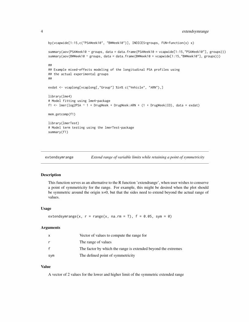
extendsymrange Extend range of variable limits while retaining a point of symmetricity

Description

This function serves as an alternative to the R function ’extendrange’, when user wishes to conservea point of symmetricity for the range. For example, this might be desired when the plot shouldbe symmetric around the origin x=0, but that the sides need to extend beyond the actual range ofvalues.

Usage

extendsymrange(x, r = range(x, na.rm = T), f = 0.05, sym = 0)

Arguments

x Vector of values to compute the range for

r The range of values

f The factor by which the range is extended beyond the extremes

sym The defined point of symmetricity

Value

A vector of 2 values for the lower and higher limit of the symmetric extended range

hmap 5

Author(s)

Teemu Daniel Laajala <[email protected]>

See Also

extendrange

Examples

set.seed(1)ex <- rnorm(10)+2

hist(ex, xlim=extendsymrange(ex, sym=0), breaks=100)

hmap Plot-region based heatmap

Description

This function plots heatmap figure based on the normal plot-region. This is useful if the image-based function ’heatmap’ is not suitable, i.e. when multiple heatmaps should be placed in a singledevice.

Usage

hmap(x, add = F,xlim = c(0.2, 0.8),ylim = c(0.2, 0.8),col = heat.colors(10),border = matrix(NA, nrow = nrow(x), ncol = ncol(x)),lty = matrix("solid", nrow = nrow(x), ncol = ncol(x)),lwd = matrix(1, nrow = nrow(x), ncol = ncol(x)),hclustfun = hclust,distfun = dist,reorderfun = function(d, w) reorder(d, w),textfun = function(xseq, yseq, labels, type = "row", ...){ if (type == "col") par(srt = 90);text(x = xseq, y = yseq, labels = labels, ...);if (type == "col") par(srt = 0)},symm = F,Rowv = NULL,Colv = if (symm) Rowv else NULL,leftlim = c(0, 0.2), toplim = c(0.8, 1),rightlim = c(0.8, 1), bottomlim = c(0, 0.2),type = "rect",scale = c("none", "row", "column"),na.rm = T,

6 hmap

nbins = length(col),valseq =seq(from = min(x, na.rm = na.rm),to = max(x, na.rm = na.rm), length.out = nbins),namerows = T,namecols = T,...)

Arguments

x Matrix to be plotted

add Should the figure be added to the plotting region of an already existing figure

xlim The x limits in which the heatmap is placed horizontally in the plotting region

ylim The y limits in which the heatmap is placed vertically in the plotting region

col Color palette for the heatmap colors

border A matrix of border color definitions (rectangles in the heatmap)

lty A matrix of line type definitions (rectangles in the heatmap)

lwd A matrix of line width definitions (rectangles in the heatmap)

hclustfun The hierarchical clustering function similar to ’stats::heatmap’ implementation.Should yield a valid ’hclust’ object for a given distance/dissimilarity matrix.

distfun The distance/dissimilarity function similar to ’stats::heatmap’ implementation.Should yield a valid ’dist’ object for a given data matrix.

reorderfun The function to use to reorder branches of the clustering (notice that same-levelbranches in a hierarchical clustering may be permutated without violating thesolution). The default approach from ’stats::heatmap’ is utilized here.

textfun A text function that is used to plot the names of the rows and columns, if de-sired. The default implementation shows how user could tailor the columns androws differently, by turning the column labels around 90-degrees. The parameter’type’ is used to distinguish between rows and columns.

symm Should the given data matrix be treated as symmetric (has to be a square matrixif so), by default ’FALSE’.

Rowv The row clustering parameter. If ’NA’ the row hierarchical clustering is com-pletely omitted. Alternatively, if a numeric vector of ranks, the ordering ofbranches is tried to be permutated according to the desired order. This can alsobe a pre-computed dendrogram-object.

Colv The column clustering parameter. If ’NA’ the column hierarchical clustering iscompletely omitted. Alternatively, if a numeric vector of ranks, the ordering ofbranches is tried to be permutated according to the desired order. This can alsobe a pre-computed dendrogram-object.

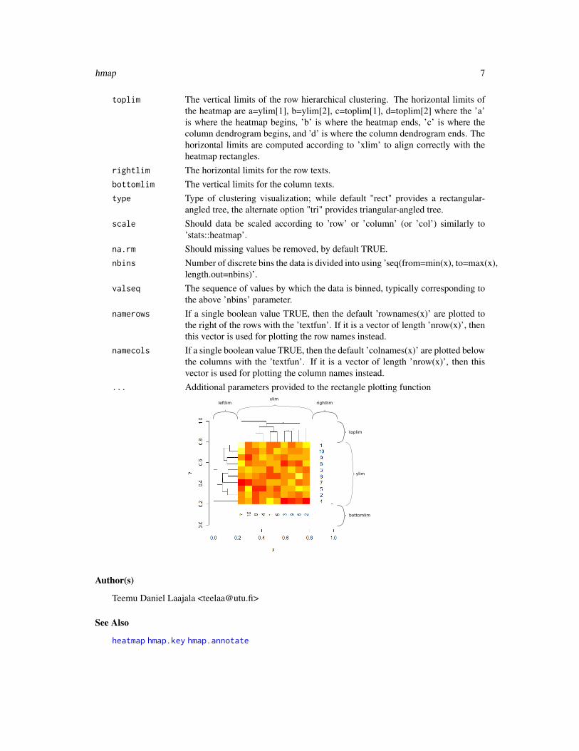
leftlim The horizontal limits of the row hierarchical clustering. The horizontal limitsof the heatmap are a=leftlim[1], b=leftlim[2], c=xlim[1], d=xlim[2] where the’a’ is where the row dendrogram begins, ’b’ is where the row dendrogram ends,’c’ is where the heatmap itself begins, and ’d’ is where the heatmap itself ends.The vertical limits are computed according to ’ylim’ to align correctly with theheatmap rectangles.

hmap 7

toplim The vertical limits of the row hierarchical clustering. The horizontal limits ofthe heatmap are a=ylim[1], b=ylim[2], c=toplim[1], d=toplim[2] where the ’a’is where the heatmap begins, ’b’ is where the heatmap ends, ’c’ is where thecolumn dendrogram begins, and ’d’ is where the column dendrogram ends. Thehorizontal limits are computed according to ’xlim’ to align correctly with theheatmap rectangles.

rightlim The horizontal limits for the row texts.bottomlim The vertical limits for the column texts.type Type of clustering visualization; while default "rect" provides a rectangular-

angled tree, the alternate option "tri" provides triangular-angled tree.scale Should data be scaled according to ’row’ or ’column’ (or ’col’) similarly to

’stats::heatmap’.na.rm Should missing values be removed, by default TRUE.nbins Number of discrete bins the data is divided into using ’seq(from=min(x), to=max(x),

length.out=nbins)’.valseq The sequence of values by which the data is binned, typically corresponding to

the above ’nbins’ parameter.namerows If a single boolean value TRUE, then the default ’rownames(x)’ are plotted to

the right of the rows with the ’textfun’. If it is a vector of length ’nrow(x)’, thenthis vector is used for plotting the row names instead.

namecols If a single boolean value TRUE, then the default ’colnames(x)’ are plotted belowthe columns with the ’textfun’. If it is a vector of length ’nrow(x)’, then thisvector is used for plotting the column names instead.

... Additional parameters provided to the rectangle plotting function

toplim

bottomlim

rightlimleftlimxlim

ylim

Author(s)


See Also

heatmap hmap.key hmap.annotate

8 hmap.annotate

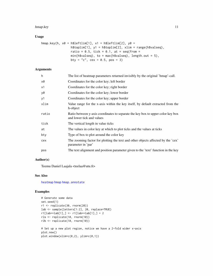
Examples

# Generate some dataset.seed(1)r1 <- replicate(30, rnorm(20))lab <- sample(letters[1:2], 20, replace=TRUE)r1[lab==lab[1],] <- r1[lab==lab[1],] + 2r2a <- replicate(10, rnorm(10))r2b <- replicate(10, rnorm(10))

# Set up a new plot region, notice we have a 2-fold wider x-axisplot.new()plot.window(xlim=c(0,2), ylim=c(0,1))

# Plot an example plot along with the color key and annotations for our 'lab' vectorh1 <- hmap(r1, add = TRUE)hmap.key(h1, x1=0.18)hmap.annotate(h1, rw = lab, rw.wid=c(0.82,0.90))

# Plot the rest to show how the coordinates are adjusted to place the heatmap(s) differentlyh2a <- hmap(r2a, add = TRUE, xlim=c(1.2, 1.8), leftlim=c(1.0, 1.2),rightlim=c(1.8,2.0), ylim=c(0.6, 1.0), bottomlim=c(0.5,0.6), Colv=NA)h2b <- hmap(r2b, add = TRUE, xlim=c(1.2, 1.8), leftlim=c(1.0, 1.2),rightlim=c(1.8,2.0), ylim=c(0.1, 0.5), bottomlim=c(0.0,0.1), Colv=NA)

# Show the normal plot region axesaxis(1, at=c(0.5,1.5), c("A", "B"))

## Not run:# Heatmap used as base for the help documentation figureset.seed(1)hmap(matrix(rnorm(100), nrow=10), xlim=c(0.2,0.8), ylim=c(0.2,0.8),leftlim=c(0.0,0.2), rightlim=c(0.8,1.0),bottomlim=c(0.0,0.2), toplim=c(0.8,1.0))axis(1); axis(2); title(xlab="x", ylab="y")

## End(Not run)

hmap.annotate Add a row and column annotations to a plot-region based heatmapbuilt with ’hmap’

Description

Annotation of rows or columns in a ’hmap’-plot. By default, rectangles aligned with either rowsor columns are plotted to the right-side or lower-side of the heatmap respectively. User-specifiedcustomizations may be given to change these annotations in positioning or type.

hmap.annotate 9

Usage

hmap.annotate(h, rw, rw.n = length(unique(rw)), rw.col = rainbow(rw.n,start = 0.05, end = 0.5), rw.wid, rw.hei, rw.pch,rw.x = rep(min(h$rightlim), times =length(h$rowtext$xseq)), rw.y = h$rowtext$yseq, rw.shift= c(0.02, 0), cl, cl.n= length(unique(cl)), cl.col = rainbow(cl.n, start =0.55, end = 1), cl.wid, cl.hei, cl.pch, cl.x =h$coltext$xseq, cl.y = rep(max(h$bottomlim), times =length(h$coltext$yseq)), cl.shift = c(0, -0.02), ...)

Arguments

h The list of heatmap parameters returned invisibly by the original ’hmap’-call.rw Annotation vector for rows ’r’, each unique instance is given a different color

(or pch) and plotted right-side of the corresponding heatmap rowsrw.n Number of unique colors (or pch) to give each annotated rowrw.col A vector for color values for unique instances in ’r’ for annotating rowsrw.wid The widths for annotation boxes for each row ’r’rw.hei The heights for annotation boxes for each row ’r’rw.pch Alternatively, instead of widths and heights user may specify a symbol ’pch’ to

use for annotating each rowrw.x The x-coordinate locations for the row annotations, by default right side of

heatmap itselfrw.y The y-coordinate locations for the row annotations, by default same vertical

locations as for the heatmap rowsrw.shift Row annotation shift: a vector of 2 values, where first indicates the amount of

x-axis shift desired and the second indicates the amount of y-axis shiftcl Annotation vector for columns ’r’, each unique instance is given a different color

(or pch) and plotted lower-side of the corresponding heatmap columnscl.n Number of unique colors (or pch) to give each annotated columncl.col A vector for color values for unique instances in ’c’ for annotating columnscl.wid The widths for annotation boxes for each column ’c’cl.hei The heights for annotation boxes for each column ’c’cl.pch Alternatively, instead of widths and heights user may specify a symbol ’pch’ to

use for annotating each columncl.x The x-coordinate locations for the column annotations, by default same horizon-

tal locations as for the heatmap columnscl.y The y-coordinate locations for the column annotations, by default lower side of

heatmap itselfcl.shift Column annotation shift: a vector of 2 values, where first indicates the amount

of x-axis shift desired and the second indicates the amount of y-axis shift... Additional parameters supplied either to ’rect’ or ’points’ function if user desired

rectangles or ’pch’-based points respectively

10 hmap.key

Author(s)


See Also

heatmap hmap.key hmap

Examples






hmap.key Add a color key to a plot-region based heatmap built with ’hmap’

Description

A continuous color scale key for a heatmap. By default the key is constructed according to the ’h’-object which is invisibly returned by the original ’hmap’-call. Some customization may be suppliedto position the legend or to customize ticks and style.

hmap.key 11

Usage

hmap.key(h, x0 = h$leftlim[1], x1 = h$leftlim[2], y0 =h$toplim[1], y1 = h$toplim[2], xlim = range(h$valseq),ratio = 0.5, tick = 0.1, at = seq(from =min(h$valseq), to = max(h$valseq), length.out = 5),bty = "c", cex = 0.5, pos = 3)

Arguments

h The list of heatmap parameters returned invisibly by the original ’hmap’-call.

x0 Coordinates for the color key; left border

x1 Coordinates for the color key; right border

y0 Coordinates for the color key; lower border

y1 Coordinates for the color key; upper border

xlim Value range for the x-axis within the key itself, by default extracted from theh-object

ratio Ratio between y-axis coordinates to separate the key box to upper color key boxand lower tick and values

tick The vertical length in value ticks

at The values in color key at which to plot ticks and the values at ticks

bty Type of box to plot around the color key

cex The zooming factor for plotting the text and other objects affected by the ’cex’parameter in ’par’

pos The text alignment and position parameter given to the ’text’ function in the key

Author(s)


See Also

heatmap hmap hmap.annotate

Examples



12 match.allocate




match.allocate Allocation of matched units to intervention arms

Description

This function allocates units belonging to a single submatch to separate intervention arms. Thisensures that the resulting intervention groups are homogeneous in respect to the variables that wereused to construct the distance/dissimilarity matrix for the non-bipartite matching. The number ofresulting intervention groups is equal to the ’g’ (i.e. submatch size) used in the multigroup non-bipartite matching.

Usage

match.allocate(xmat)

Arguments

xmat A binary matching matrix or a matching vector given by match.bb-function.

Value

A vector where each element indicates to which group the observation was randomized to. Thegroup names are "Group_A", "Group_B", "Group_C", ... until ’g’ letters, where ’g’ was the size ofsubmatches.

Author(s)


See Also

match.bb match.mat2vec match.vec2mat match.dummy

match.bb 13

Examples

data(vcapwide)

# Construct an Euclidean distance example distance matrix using 15 observations from the VCaP studyd <- as.matrix(dist(vcapwide[1:15,c("PSAWeek10", "BWWeek10")]))# Matching using the b&b algorithm to submatches of size 3# (which will result in 3 intervention groups)bb3 <- match.bb(d, g=3)str(bb3)


# Perform an example random allocation of the above submatches,# these will be randomly allocated to 3 arms based on the submatchesset.seed(1)groups <- match.allocate(solvec)

# Illustrate randomization, no baseline differences in these three artificial groupsby(vcapwide[1:15,c("PSAWeek10", "BWWeek10")], INDICES=groups, FUN=function(x) x)

summary(aov(PSAWeek10 ~ groups, data = data.frame(PSAWeek10 = vcapwide[1:15,"PSAWeek10"], groups)))summary(aov(BWWeek10 ~ groups, data = data.frame(BWWeek10 = vcapwide[1:15,"BWWeek10"], groups)))

match.bb Branch and Bound algorithm implementation for performing multi-group non-bipartite matching

Description

This function performs multigroup non-bipartite matching of observations based on a provided dis-tance/dissimilarity matrix ’d’. The number of elements in each submatch is defined by the parameter’g’.

Usage

match.bb(d, g = 2, presort = "complete", progress = 1e+05,bestknown = Inf, maxbranches = Inf, verb = 0)

Arguments

d A distance matrix with NxN elements

g Number of elements per each submatch, i.e. how many observations are alwaysmatched together

presort If hierarchical clustering should be used for an initial guess, hclust method-options are valid options ("complete", "single", "ward", "average")

progress How many branching operations are done before outputting information to theuser

14 match.bb

bestknown If a best known solution already exists, this can be used to bound branches ofthe tree before initiation. The default Inf value causes whole search tree to bepotential solution space.

maxbranches Maximum number of branching operations before returning current best solu-tion, by default no cutoff is defined.

verb Level of verbosity

Details

See further details in the reference Laajala et al.

Value

The function returns a list of objects, where elements are

branches Number of branching operations during the branch and bound algorithm

bounds Number of bounding operations during the branch and bound algorithm

ends Number of end leaf nodes visited during the branch and bound algorithm

matrix The resulting binary matching matrix where rows and columns sum to g

solution The resulting matching vector where each element indicates the submatch wherethe observation was placed

cost Final cost value of the target function in the minimization task

Note

Notice that the solution submatch vector in $solution is not the same as the intervention groupallocation. Submatches should be randomly allocated to intervention arms using the match.allocate-function.

The package ’nbpMatching’ provides a FORTRAN implementation for computation of paired non-bipartite matching case (g=2).

Computation may be heavy if the number of observations is high, or the number of within-submatchpairwise distances to consider is high (increases quadratically as a function of ’g’).

Author(s)


See Also

match.allocate match.mat2vec match.vec2mat match.dummy

Examples

data(vcapwide)

# Construct an Euclidean distance example distance matrix using 15 observations from the VCaP studyd <- as.matrix(dist(vcapwide[1:15,c("PSAWeek10", "BWWeek10")]))

match.dummy 15

bb3 <- match.bb(d, g=3)str(bb3)

mat <- bb3$matrix# binary matching matrixsolvec <- bb3$solution# matching vector, where each element indicates to which submatch each observation belongs to

mixplot(data.frame(vcapwide[1:15,c("PSAWeek10", "BWWeek10")],submatch=as.factor(paste("Submatch_",solvec, sep=""))), pch=16, col=rainbow(5))

match.dummy Create dummy individuals or sinks to a data matrix or a dis-tance/dissimilarity matrix

Description

Dummy observations are allowed in order to make the number of observations dividable by thenumber of elements in each submatch, i.e. for pairwise matching the number of observations shouldbe paired, for triangular matching the number of observations should be dividable by 3, etc. Thiscan be done either by adding column averaged individuals to the original data frame (parameter’dat’), or by adding zero distance sinks to the distance/dissimilarity matrix (parameter ’d’). Thelatter approach favors dummies being matched to real extreme observations, while the former favorsdummies being matched to close-to-mean real observations.

Usage

match.dummy(dat, d, g = 2)

Arguments

dat A data.frame of the original observations, to which column averaged new dummyobservations are added

d N times N distance/dissimilarity matrix, to which zero distance sinks are added

g The desired number of elements per each submatch, i.e. the size of the clusters.The number of added dummies is the smallest number of additions that fulfills(N+dummy)%%g == 0

Value

Depending on if the dat or the d parameter was provided, the function either: dat: adds new averagedindividuals according to column means and then returns the data matrix d: adds zero distance sinksto the distance/dissimilarity matrix and returns the new distance/dissimilarity matrix

Note

Adding zero distance sinks to the distance matrix or averaged individuals to the original data frameproduce different results and affect the optimal matching task differently.

16 match.ga

Author(s)


See Also

match.allocate match.mat2vec match.vec2mat match.bb

Examples

data(vcapwide)

exdat <- vcapwide[1:10,c("PSAWeek10", "BWWeek10")]dim(exdat)avgdummies <- match.dummy(dat=exdat, g=3)dim(avgdummies)# Construct an Euclidean distance matrix after adding two dummy individuals# (averaged individuals to the original data matrix)bb3 <- match.bb(as.matrix(dist(avgdummies)), g=3)str(bb3)

# Construct an Euclidean distance matrix after adding two dummy distances (zero distance sinks)exd <- as.matrix(dist(vcapwide[1:10,c("PSAWeek10", "BWWeek10")]))dim(exd)d <- match.dummy(d=exd, g=3)dim(d)# 10 is not dividable by 3, 2 sinks are added to make d 12x12bb3 <- match.bb(d, g=3)str(bb3)

# Notice that sinks produce a lot smaller target function costs than averaged individuals

match.ga Non-bipartite matching using the Genetic Algorithm (GA)

Description

An implementation of the Genetic Algorithm for solving non-bipartite matching tasks with cus-tomizable evolutionary events and parameters

Usage

match.ga(d, g,pops,generations = 100,popsize = 100,nmutate = 100,ndeath = 30,type = "min",mutate = hamlet:::.ga.mutate,

match.ga 17

breed = hamlet:::.ga.breed,weight = hamlet:::.ga.weight,fitness = hamlet:::.ga.fitness,step = hamlet:::.ga.step,initialize = hamlet:::.ga.init,progplot = T,plot = T,verb = 0,progress = 500,...)

Arguments

d A distance/dissimilarity matrix ’d’

g The size in submatches, as in how many observations are always connected

pops If user wants to specify starting populations, they can be provided here as amatrix. Each row correspondings to the observations, while columns are thedifferent solutions (population in the GA). For example, a 10 row 100 columnpops-matrix would be 100 different matching solutions of 10 observations. Eachnumber in the matrix indicates a different submatch.

generations Number of simulations to run in the GA. In each step, mutations, breeding andbreeding occur according to user’s specified settings, and a new generation iscreated out of this.

popsize Number of solutions (=’individuals’) to have in each step of the algorithm.

nmutate Number of mutations to occur in each step. Individuals are sampled with re-placement, and then given the corresponding number of mutations.

ndeath Number of deaths to occur in each step. Each dead solution (=’individual’)is then replaced by breeding suitable parents (probability of being a parentweighted by fitness).

type Type of optimization, can be ’min’ or ’max’.

mutate Mutation function; by default the hamlet internal function ’.ga.mutate’ is used.This function takes in solution vector ’x’. Two random positions are then swapped,which could be seen as a form of a point mutation.

breed Breeding function; by default the hamlet internal function ’.ga.breed’ is used.This function takes in solution vectors ’x’ and ’y’ ,which will be the parents,and the distance matrix ’d’. The products x*d and y*d are computed, and row-wise differences are computed between the two matrices. The row with thehighest difference indicates where one of the parents can be most improved, andthis trait is inherited from the other parent.

weight Weighting function; by default the hamlet internal function ’.ga.weight’ is used.This weight should be correspond to probabilities that the corresponding indi-viduals will undergo some sort of event (i.e. mutation, death) or participate inproducing offspring (i.e. breed). This probability weight is computed accordingto ranks of fitnesses computed in the

18 match.ga

fitness Fitness function; by default the hamlet internal function ’.ga.fitness’ is used.This should yield the numeric fitness for a solution, indicating how viable thesolution is in relation to the others. In a minimization task the lower fitnessindicates better viability.

step A step function; by default the hamlet internal function ’.ga.step’ is used. Thestep function which combines all operations in the GA, in order to produce thenext generation of solutions given the previous one.

initialize Initialization function; by default the hamlet internal function ’.ga.initialize’ isused. This function should format a set of valid solutions to produce the firstgeneration in the beginning of the GA.

progplot Should progress be plotted. If true, in every generation index dividable by theparameter ’progress’, a function of fitnesses over the generations is plotted. Theplot shows development of solution cost quantiles over time.

plot Should the function plot the final quantiles over all the generations.

verb Level of verbosity; -1 indicates omitting of verbal output, 0 indicates normallevel, and +1 indicates debugging/additional information.

progress How often should the function plot and print intermediate information on theprogress.

... Additional parameters for the internal GA functions.

Details

The Genetic Algorithm (GA) is a form of an evolutionary optimization algorithm, where a popula-tion (a group of solutions to an optimization tasks) reproduce among themselves, die, mutate, andlive on in a simulated environment. As the GA is a generic framework of solution approaches, ithas many adjustable parameters and user may wish to explore many different options for the pop-ulations (for example in population size, mutation frequencies, fitness functions, drift etc) and alsothe evolutionary mechanics (such as breeding technique, types of mutations, and suitability for re-producing). Here, general default options and mechanics are provided, but it is advisable to exploredifferent parameters for the particular optimization task in hand to find optimal solutions. If the userwishes to explore the implementation of the default mechanics, the function implementations areinternally available in the hamlet-package. For example, the mutation function is accessible withthe command: ’ hamlet::.ga.mutate ’.

Value

The returned list compromises of:

• A list of solutions; a matrix ’pops’ which contains the population of solutions in the finalgeneration of the algorithm, a vector ’fitnesses’ which portrait the corresponding fitnesses tothe columns of ’pops’, and ’weights’ which were the corresponding probabilities to events inthe GA.

• A vector ’bestsol’, for which the fitness function obtained minimum (or maximum) valueduring the algorithm.

• A value ’best’, which is the optimum solution cost value observed during the algorithm.

match.mat2vec 19

Note

Notice that end quality of the matching based allocation is heavily dependent on providing a feasiblematrix D. One should carefully consider choice and tuning of the similarity metric. For example,Euclidean distance without standardization is often not a good choice as it does not normalize thevariance of each variable and emphasis is on baseline variables that have a large relative variance.

Note that the R-package ’GA’ offers a wide range of generalized GA-related tools.

Author(s)


See Also

match.bb

Examples

# Set up a distance matrix and add dummies, then run GAdata(vcapwide)

# Construct an Euclidean distance example distance matrix using 15 observations from the VCaP studyd <- as.matrix(dist(vcapwide[1:15,c("PSAWeek10", "BWWeek10")]))# Or rather, z-score transform all input variables firstd2 <- as.matrix(dist(scale(vcapwide[1:15,c("PSAWeek10", "BWWeek10")])))

# Notice that random simulations take place, so we will fix the RNG seed for reproducibilityset.seed(1)# Resulting genetic algorithm progression is plotted by defaultga <- match.ga(d2, g=3, generations=60)str(ga)# Submatches, i.e. similar individuals that ought to be allocated to separate groupsga[[2]]

match.mat2vec Transform a binary matching matrix to a matching vector

Description

This function transforms a binary matching matrix to a matching vector. A matching vector is oflength N where each element indicates the submatch to which the observation belongs to. No-tice that this is not the same as the group allocation vector that is provided by the match.allocate-function. The binary matching matrix is of size N x N where 0 indicates that the observations havebeen part of a different submatch, and 1 indicates that the observations have been part of the samesubmatch. Diagonal is always 0 although an observation is always in the same submatch with itsself.

20 match.mat2vec

Usage

match.mat2vec(xmat)

Arguments

xmat A binary matching matrix ’xmat’

Value

A matching vector where each element indicates submatch the observation belongs to

Note

Notice that the particular index numbers produced by match.mat2vec may be different to that of thebranch and bound solution vector, but that the submatches shared by observations are common.

Author(s)


See Also

match.allocate match.bb match.vec2mat match.dummy

Examples

data(vcapwide)



mat <- bb3$matrix# matching vector, where each element indicates to which submatch each observation belongs to

matsolvec <- match.mat2vec(mat)which(mat[1,] == 1)# E.g. the first, third and thirteenth observation are part of the same submatchwhich(solvec == solvec[1])# Similarly

match.vec2mat 21

match.vec2mat Transform a matching vector to a binary matching matrix

Description

This function allows transforming a matching vector to a binary matching matrix. A matchingvector is of length N where each element indicates the submatch to which the observation belongs to.Notice that this is not the same as the group allocation vector that is provided by the match.allocate-function. The binary matching matrix is of size N x N where 0 indicates that the observations havebeen part of a different submatch, and 1 indicates that the observations have been part of the samesubmatch. Diagonal is always 0 although an observation is always in the same submatch with itsself.

Usage

match.vec2mat(x)

Arguments

x A matching vector ’x’

Value

N times N binary matching matrix, where 0 indicates that the observations have been part of adifferent submatch, and 1 indicates that the observations have been part of the same submatch.

Author(s)


See Also

match.allocate match.mat2vec match.bb match.dummy

Examples

data(vcapwide)




solvecmat <- match.vec2mat(solvec)

22 mem.getcomp

matwhich(mat[1,] == 1)# E.g. the first, third and thirteenth observation are part of the same submatchwhich(solvec == solvec[1])# Similarly

mem.getcomp Extract per-observation components for fixed and random effects of amixed-effects model

Description

Assuming a mixed-effects model of form y_fit = Xb + Zu + e, where X is the model matrix forfixed effects, Z is the model matrix for random effects, and b and u are the fixed and random effectsrespectively, this function returns these components per each fitted value y. These may be useful formodel inference and/or diagnostic purposes.

Usage

mem.getcomp(fit)

Arguments

fit A fitted mixed-effects model generated either through the lme4 or the nlme pack-age.

Details

Notice that per-observation model error is e = Xb + Zu - y_observation. Similarly, the componentsXb and Zu are extracted.

Value

The function returns per-observation model fit components for a mixed-effects model. The returnfields are

Xb Fixed effects component Xb

Zu Random effects component Zu

XbZu Full model fit by summing the above two Xb+Zu

e Model error e

y Original observations y

Author(s)


mem.plotran 23

See Also

mem.plotran mem.plotresid

Examples

data(vcaplong)


library(lme4)f1 <- lmer(log2PSA ~ 1 + DrugWeek + DrugWeek:ARN + (1 + DrugWeek|ID), data = exdat)

mem.getcomp(f1)

mem.plotran Plot random effects histograms for a fitted mixed-effects model

Description

This plot creates histogram plots for the columns extracted from random effects from a model fit.This is useful for model diagnostics, such as observing deviations from normality in the randomeffects.

Usage

mem.plotran(fit, breaks = 100)

Arguments


breaks Number of breaks in the histograms (passed to the ’hist’-function)

Author(s)


See Also

mem.getcomp, mem.plotresid

24 mem.plotresid

Examples

data(vcaplong)


library(lme4)f1 <- lmer(log2PSA ~ 1 + DrugWeek + DrugWeek:ARN + (1 + DrugWeek|ID), data = exdat)

ranef(f1) # Histograms are plotted for these columnsmem.plotran(f1)

mem.plotresid Plot residuals of a mixed-effects model along with trend lines

Description

This function plots stylized residuals of a mixed-effects model. It is possible to obtain fitted valuesversus errors (XbZu vs e), or original values versus errors (y vs e) in order to obtain different viewsto the errors in connection to the observations.

Usage

mem.plotresid(fit, linear = T, type = "XbZu", main, xlab, ylab)

Arguments


linear Should linear trend lines be drawn to the residual plot

type Type of residual plot; should fitted values (value "XbZu") or original observa-tions (value "y") be plotted against "e" errors

main Main title

xlab x-axis label

ylab y-axis label

Details

Notice that the typical residual plot is fitted values (type="XbZu") versus errors ("e").

Author(s)


See Also

mem.getcomp, mem.plotran

mem.powersimu 25

Examples

data(vcaplong)


library(lme4)f0 <- lmer(log2PSA ~ 1 + DrugWeek + (1 + DrugWeek|ID), data = exdat)f1 <- lmer(log2PSA ~ 1 + DrugWeek + DrugWeek:ARN + (1 + DrugWeek|ID), data = exdat)f2 <- lmer(log2PSA ~ 1 + DrugWeek + DrugWeek:ARN + (1|ID) + (0 + DrugWeek|ID), data = exdat)f3 <- lmer(log2PSA ~ 1 + DrugWeek + DrugWeek:ARN + (1|Submatch) + (0 + DrugWeek|ID), data = exdat)

par(mfrow=c(2,2))mem.plotresid(f0)mem.plotresid(f1)mem.plotresid(f2)mem.plotresid(f3)

mem.powersimu Power simulations for the fixed effects of a mixed-effects modelthrough structured bootstrapping of the data and re-fitting of the model

Description

Bootstrap sampling is used to investigate the statistical significance of the fixed effects terms speci-fied for a readily fitted mixed-effects model as a function of the number of individuals participatingin the study. User either specifies a suitable sampling unit, or it is automatically identified based onthe random effects formulation of a readily fitted mixed-effects model. Per each count of individu-als in vector N, a fixed number of bootstrapped datasets are generated and re-fitted using the modelformulation on the pre-fitted model. Power is then computed as the fraction of effects identified asstatistically significant out of all the bootstrapped datasets.

Usage

mem.powersimu(fit, N = 4:20, boot = 100, level = NULL, strata = NULL,default = FALSE, seed = NULL, plot = TRUE, plot.loess = FALSE,legendpos = "bottomright", return.data = FALSE, verb = 1, ...)

Arguments

fit A fitted mixed-effects model. Should be either a model produced by the lme4-package, or then a modified lme4-fit such as provided by lmerTest or similarpackage that builds on lme4.

N A vector of desired amounts of individuals to be tested, i.e. sample sizes N.Notice that the N may be either a total N if no strata is spesified, or then an Nvalue per each substrata if strata is not NULL. See below the parameter ’strata’.

boot Number of bootstrapped datasets to generate per each N value. The total numberof generated data frames in the end will be N times boot.

26 mem.powersimu

level An unambiguous indicator available in the model data frame that indicates eachseparate individual unit in the experiment. For example, this may correspondto a single patient indicator column ID, where each patient has a unique IDinstance. If this parameter is given as NULL, then this function automaticallyattempts to identify the best possible level of individual indicators based on therandom effects specified for the model.

strata If any sampling strata should be balanced, it should be indicated here. For ex-ample, if one is studying the possible effects of an intervention, it is typical tohave an equal number of individual both in the control and in the interventionarms also in the sampled datasets. It should be then given as an column nameavailable in the original model data frame. Each strata will be sampled in equalamounts.

default What is the default statistical significance if a model could not be re-fitted to thesampled datasets, which may occur for example due to convergence or redun-dance issues. This defaults to FALSE, which means that a coefficient is expectedto be statistically insignificant if the corresponding model re-fitting fails in lme4.

seed For reproducibility, one may wish to set a numeric seed to produce the exactsame results.

plot If set to TRUE, the function will plot a power curve. Each fixed effects coeffi-cient is a different curve, with color coding and a legend annotated to separatewhich one is which.

plot.loess If plot==TRUE, this plot.loess==TRUE adds an additional loess-smoothed ap-proximated curve to the existing curves. This is useful if running the simulationswith a low number of bootstrapped samples, as it may help approximate wherethe curve reaches critical points, i.e. power = 0.8.

legendpos Position for the legend in plot==TRUE, defaults to "bottomright". Any legalposition similar to provided the function ’legend’ is allowed.

return.data Should one obtain the bootstrapped data instead of bootstrapping and then re-fitting. This will skip the model re-fitting schema and instead return a list of listswith the bootstrapped data instead. The outer list corresponds to the values of’N’, while the inner loop corresponds to the different ’boot’ runs of bootstrap.This may be useful to inspecting that the schema is sampling correct samplingunits for example, or if bootstrapping is to be used for something else than re-fitting the lme4-models.

verb Numeric value indicating the level of verbosity; 0=silent, 1=normal, 2=debug-ging.

... Additional parameters provided for the function.

Details

This function will by default utilizes the lmerTest-package’s Satterthwaite approximation for deter-mining the p-values for the fixed effects. If this fails, it resorts to the conventional approximation|t|>2 for significance, which is not accurate, but may provide a reasonable approximation for thepower levels.

mix.binary 27

Value

If return.data==FALSE, this function will return a matrix, where the rows correspond to the differentN values and the columns correspond to the fixed effects. The values [0,1] are the fraction ofbootstrapped datasets where the corresponding fixed effects was detected as statistically significant.

Note

Please note that the example runs in this document are extremely small due to run time constraintson CRAN. For real power analyses, it is recommended that the N counts would vary e.g. from 5 to15 with steps of 1 and the amount of bootstrapped datasets would be at least 100.

Author(s)

Teemu D. Laajala

See Also

mem.getcomp

Examples

# Use the VCaP ARN data as an exampledata(vcaplong)arn <- vcaplong[vcaplong[,"Group"] == "Vehicle" | vcaplong[,"Group"] == "ARN",]

# lme4 is required for mixed-effects modelslibrary(lme4)# Fit an example fixed effects modelfit <- lmer(PSA ~ 1 + DrugWeek + ARN:DrugWeek + (1|ID) + (0 + DrugWeek|ID), data = arn)

# For reproducibility, set a seedset.seed(123)# Run a brief power analysis with only a few selected N values and a limited number of bootstrapping# Balance strata over the ARN and non-ARN (=Vehicle) so that both contain equal count of individualspower <- mem.powersimu(fit, N=c(3, 6, 9), boot=10, strata="ARN", plot=TRUE)# Power curves are plotted, along with returning the power matrix at:power

# Notice that each column corresponds to a specified fixed effects at the formula# "1 + DrugWeek + ARN:DrugWeek"

mix.binary Binary coding of categorical variables

Description

This function encodes categorical variables (e.g. columns of type ’factor’ or ’character’). U newcolumns are created per each such column, where U is the number of unique instances of thatcolumn. The new columns are named OriginalColumnName_U1, OriginalColumnName_U2, etc.

28 mix.fun

Usage

mix.binary(x)

Arguments

x A data.frame or a matrix where categorical columns are to be binary coded.Categorical columns are assumed to be all non-numeric fields.

Details

A function that codes categorical variables in a dataset into binary variables. This is done in thefollowing manner: e.g. x = red, green, blue, green –> x_new = 1,0,0, 0,1,0, 0,0,1, 0,1,0 where thedimensions in x_new are is_red, is_green and is_blue

Value

The function returns a data.frame, where categorical variables have been replaced with 0/1-binaryfields, and numeric fields have been left untouched. Notice that the order of the columns may notbe the original.

Author(s)


Examples

data(vcapwide)

ex <- mix.binary(vcapwide[,c("Group", "CastrationDate")])apply(ex, MARGIN=1, FUN=sum)# Notice that each row sums to 2, as two categorical variables were binary coded# and no missing values were present

mix.binary(vcapwide[,c("PSAWeek4", "Group", "CastrationDate")])# Binary coding is only applied to non-numeric fields

mix.fun Apply function to numerical columns of a mixed data.frame while ig-noring non-numeric fields

Description

This function is intended for applying functions to numeric fields of a mixed type data.frame.Namely, the function ignores fields that are e.g. factors, and returns FUN function applied to onlythe numeric fields.

Usage

mix.fun(x, FUN = scale, ...)

mixplot 29

Arguments

x Data.frame x with mixed type fields

FUN Function to apply, for example ’scale’, ’cov’, or ’cor’

... Additional parameters passed on to FUN

Value

Return values of FUN when applied to numeric columns of ’x’

Author(s)


See Also

apply

Examples

data(vcapwide)

mix.fun(vcapwide[,c("Group", "PSAWeek4", "PSAWeek10", "PSAWeek14")], FUN=scale)# Column 'Group' is ignoredmix.fun(vcapwide[,c("Group", "PSAWeek4", "PSAWeek10", "PSAWeek14")], FUN=cov, use="na.or.complete")# ... is used to pass the 'use' parameter to the 'cov'-function

mixplot Scatterplot for mixed type data

Description

This function plots a scatterplot similar to the default plot-function, with the difference that fac-tor/character fields in input data.frame are handled as categorical variables. These categorical vari-ables are color-coded and handled separately in marginal distributions.

Usage

mixplot(x,main = NA,match,func = function(x, y, par){ segments(x0 = x[1], y0 = x[2], x1 = y[1], y1 = y[2], col = par)},legend = T,col = palette(), na.lines = T,origin = F,marginal = F,lhei,

30 mixplot

lwid,verb = 0,...)

Arguments

x A data.frame or a matrix of observations. Typically x should be a data.frame,where columns are of different types, e.g. some of ’numeric’ and some of ’fac-tor’ class.

main Main title plotted on top of the figure

match A matching matrix (e.g. produced by hamlet::match.vec2mat) or a matchingvector (e.g. produced by hamlet::match.mat2vec) that indicates with differentvalues if certain observations should be connected.

func The function to apply to each pair of observations ’x’ and ’y’. By default, it isa segment line in 2 dimensions (each individual bivariate panel). Segment linecolor is indicated by the matching vector or individual element in the matchingmatrix. Thus 0-values indicate no line, while other values are used to annotatesubmatches. ’par’ is the index of the submatch, and by default indicate thecolors.

legend Should an automated legend be generated

col Colors per observation

na.lines Should lines be drawn to represent one of the variables if the other one is missingin a 2-dim scatterplot

origin Should the origin x=0, y=0 be separately indicated using lines

marginal Should marginal distributions be drawn in sides of each scatterplot

lhei Heights for bins in the layout

lwid Widths for bins in the layout

verb Level of verbosity: -1<= (no verbosity), 0/FALSE (warnings) or >=1/TRUE(additional information)

... Additional parameters given to the plot-function

Value

An invisible return of the measurements and plot layout structure (matrix, heights, and widths)

Author(s)


Examples

data(vcapwide)

mixplot(vcapwide[,c("Group", "PSAWeek4", "PSAWeek10", "PSAWeek14")], marginal=TRUE, pch=16,main="PSA at weeks 4, 10 and 14 per intervention group")

orxlong 31

orxlong Long-format longitudinal data for the ORX study

Description

Long-format measurements of PSA over the intervention period in the ORX study. Notice that thisdata.frame is in suitable format for mixed-effects modeling, where each row should correspond to asingle longitudinal measurement. These measurements are annotated using the individual indicatorfields ’ID’, time fields ’Day’, ’TrDay’, ’Date’, and the response values are contained in raw formatin ’PSA’ or after log2-transformation in ’log2PSA’. Additional fields are provided for group testingand matched inference in ’Group’, ’Submatch’, and the binary indicators ’ORX+Tx’, ’ORX’, and’Intact’.

Usage

data("orxlong")

Format

A data frame with 392 observations on the following 11 variables.

ID A unique character indicator for the different individual(s)

PSA Raw longitudinal PSA measurement values in unit (ug/l)

log2PSA Log2-transformed longitudinal PSA measurement values in unit (log2 ug/l)

Day Day since the first PSA measurement. Notice that there is a single time point prior to interven-tions.

TrDay Day since the interventions began, 0 annotating the point at which surgery was performedor drug compounds were first given.

Date A date format when the actual measurement was performed

Group The actual intervention groups, after blinded groups were assigned to ’ORX+Tx’, ’ORX’,or ’Intact’

Submatch The submatches that were assigned based on the baseline variables.

‘ORXTx’ A binary indicator field indicating which measurements belong to the group ’ORX+Tx’

ORX A binary indicator field indicating which measurements belong to the group ’ORX’

Intact A binary indicator field indicating which measurements belong to the group ’Intact’

Details

For mixed-effects modeling, the fields ’ID’, ’PSA’ (or ’log2PSA’), ’TrDay’, and group-specificindicators should be included.

32 orxlong

Note

Group-testing should be performed so that ’ORX+Tx’ is tested against ’ORX’, in order to inferpossible effects occurring due to ’Tx’ on top of ’ORX’. ’ORX’ should be compared to ’Intact’, inorder to infer if the ’ORX’ surgical procedure has beneficial effects in comparison to intact animals.For statistical modeling of the intervention effects, one should use observations with the positive’TrDay’-values, as this indicates the beginning of the interventions.

Source


Examples

data(orxlong)# Construct data frames that can be used for testing pairwise group contrastsorxintact <- orxlong[orxlong[,"Intact"]==1 | orxlong[,"ORX"]==1,c("PSA", "ID", "ORX", "TrDay", "Submatch")]orxtx <- orxlong[orxlong[,"ORXTx"]==1 | orxlong[,"ORX"]==1,c("PSA", "ID", "ORXTx", "TrDay", "Submatch")]# Include only observations occurring post-surgeryorxintact <- orxintact[orxintact[,"TrDay"]>=0,]orxtx <- orxtx[orxtx[,"TrDay"]>=0,]

# Example fitslibrary(lme4)library(lmerTest)# Conventional model fitsfit1a <- lmer(PSA ~ 1 + TrDay + ORXTx:TrDay + (1|ID) + (0 + TrDay|ID), data = orxtx)fit1b <- lmer(PSA ~ 1 + TrDay + ORXTx:TrDay + (1 + TrDay|ID), data = orxtx)fit2a <- lmer(PSA ~ 1 + TrDay + ORX:TrDay + (1|ID) + (0 + TrDay|ID), data = orxintact)fit2b <- lmer(PSA ~ 1 + TrDay + ORX:TrDay + (1 + TrDay|ID), data = orxintact)

# Collate to matched inference for pairwise observations over the submatchesmatched.orx <- do.call("rbind", by(orxintact, INDICES=orxintact[,"Submatch"], FUN=function(z){z[,"MatchedPSA"] <- z[,"PSA"] - z[z[,"ORX"]==0,"PSA"]z <- z[z[,"ORX"]==1,]z}))# Few examples of matched fits with different model formulationsfit.matched.1 <- lmer(MatchedPSA ~ 0 + TrDay + (1|ID) + (0 + TrDay|ID), data = matched.orx)fit.matched.2 <- lmer(MatchedPSA ~ 1 + TrDay + (1|ID) + (0 + TrDay|ID), data = matched.orx)fit.matched.3 <- lmer(MatchedPSA ~ 1 + TrDay + (1 + TrDay|ID), data = matched.orx)summary(fit.matched.1)summary(fit.matched.2)summary(fit.matched.3)# We notice that the intercept term is highly insignificant# if included in the matched model, as expected by baseline balance.# In contrast, the matched intervention growth coefficient is highly# statistically significant in each of the models.

orxwide 33

orxwide Wide-format baseline data for the ORX study

Description

This data frame contains the wide-format data of the ORX study for baseline characteristics of theindividuals participating in the study. Some fields (Volume, PSA, High, BodyWeight, PSAChange)were used to construct the distance matrix in the original matching-based random allocation ofindividuals at baseline, while other variables (Group, Submatch) contain these results.

Usage

data("orxwide")

Format


ID A unique character indicator for the different individual(s)Group After identifying suitable submatches, the data were distributed to blinded intervention

groups. These groups were later then annotated to actual treatments or non-intervention con-trol groups.

Submatch Submatches identified at baseline using the methodology presented in this packageVolume Tumor volume at baseline in cubic millimetersPSA Raw baseline PSA measurement values in unit (ug/l)High The highest dimension in the tumor in millimeters, giving insight into the shape of the tumorBodyWeight Body weight at baseline in unit (g)PSAChange A fold-change like change in PSA from the prior measurement defined as: (PSA_current

- PSA_last)/(PSA_last)

Details

Originally, 3-fold weighting of the baseline ’Volume’ and ’PSA’ was used in comparison to ’High’,’BodyWeight’ and ’PSAChange’ when computing the distance matrix. Furthermore, some individ-uals were annotated prior to matching for exclusion based on outlierish behaviour. The exclusioncriteria were applied before any interventions were given or the matching was performed. Theexcluded tumors had either non-existant PSA, non-detectable tumor volume, or extremely largetumors (volume above 700 mm^3).

Note

Notice that while normally the submatches would be distributed equally to the experiment groups,here rarely a single submatch may hold multiple instances from a single group. This is due topractical constraints in the experiment, that animals had to be manually moved in order to fulfillgroups and to reflect the amount of drug compounds available. Additionally, the original experimentwas performed on 6 intervention groups, while here only 3 are further presented after the baseline(’ORX+Tx’, ’ORX’ and ’Intact’).

34 smartjitter

Source


Examples

data(orxwide)# Construct an example distance matrix based on conventional# Euclidean distance and the baseline characteristicsd.orx <- dist(orxwide[,c("Volume", "PSA", "High", "BodyWeight", "PSAChange")])# Plot a hierarchical clustering of the individualsplot(hclust(d=d.orx))# This 'd.orx' may then be further processed by downstream experiment# design functions such as match.ga, match.bb, etc.

smartjitter Smart jittering function for deterministic shifting of overlapping val-ues

Description

This function takes in a vector of measurements and computes overlapping bins of observations,and applies a jittering function within each overlapping bin.

Usage

smartjitter(x, q = seq(from = 0, to = 1, length.out = 10), type = 1,amount = 0.1, jitterfuncs = list(function(n) {

(1:n)/(1/amount)}, function(n) {

(((-1)^c(0:(n - 1))) * (0:(n - 1)))/(1/amount)}), jits = jitterfuncs[[type]])

Arguments

x The values that should be jittered. Notice that these are used to determine whichare overlapping, and should not be though of as x-axis positions (see example).

q Probability quantiles where the ends of the bins should be placed

type Type of jittering, by default it is used to choose which element (1 or 2) of thelist of jittering functions is chosen as the final jittering function. Customizedfunctions may be provided to the jitterfuncs-parameter.

amount Amount of jittering (here deterministic shifting) for the jittering function

jitterfuncs List of possible jittering functions for n overlapping values. The jittering func-tion at list position ’type’ is chosen

jits Final jittering function from the jitterfuncs-list

vcaplong 35

Details

The smart jittering is applied to the x-parameter values, and returns a vector of shifting amountsper each observation. Notice that in the typical case, parameter ’x’ are the desired response valuese.g. among the y-axis, and the returned value of smartjitter are the amounts of jittering done on thex-axis of a plot.

Value

The function returns a vector of values with same length as x. The values in this vector indicatewhat should be the shifting per each observation, if the observations should be jittered along ananother axis.

Author(s)


Examples

data(vcapwide)

plot.new()plot.window(xlim=extendrange(c(0,1)), ylim=extendrange(vcapwide[,"PSAWeek4"]))y1 <- vcapwide[vcapwide[,"CastrationDate"]=="100413","PSAWeek4"]y2 <- vcapwide[vcapwide[,"CastrationDate"]=="170413","PSAWeek4"]points(x=0+smartjitter(y1, type=2, amount=0.02), y=y1)points(x=1+smartjitter(y2, type=2, amount=0.02), y=y2)axis(1, at=c(0,1), labels=c("10.04.13", "17.04.13"))axis(2); box()title(ylab="PSA at week 4", xlab="Castration batches")

vcaplong Long-format data of the Castration-resistant Prostate Cancer experi-ment using the VCaP cell line.

Description

The long-format of the VCaP experiment PSA-measurements may be used to model longitudinalmeasurements during interventions (Vehicle, ARN, or MDV). Body weights and PSA were mea-sured weekly during the experiment. PSA concentrations were log2-transformed to make data betternormally distributed.

Usage

data(vcaplong)

36 vcaplong

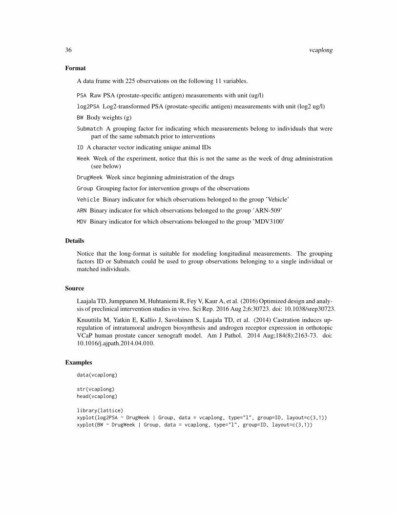
Format


PSA Raw PSA (prostate-specific antigen) measurements with unit (ug/l)

log2PSA Log2-transformed PSA (prostate-specific antigen) measurements with unit (log2 ug/l)

BW Body weights (g)

Submatch A grouping factor for indicating which measurements belong to individuals that werepart of the same submatch prior to interventions

ID A character vector indicating unique animal IDs

Week Week of the experiment, notice that this is not the same as the week of drug administration(see below)

DrugWeek Week since beginning administration of the drugs

Group Grouping factor for intervention groups of the observations

Vehicle Binary indicator for which observations belonged to the group ’Vehicle’

ARN Binary indicator for which observations belonged to the group ’ARN-509’

MDV Binary indicator for which observations belonged to the group ’MDV3100’

Details

Notice that the long-format is suitable for modeling longitudinal measurements. The groupingfactors ID or Submatch could be used to group observations belonging to a single individual ormatched individuals.

Source



Examples

data(vcaplong)

str(vcaplong)head(vcaplong)

library(lattice)xyplot(log2PSA ~ DrugWeek | Group, data = vcaplong, type="l", group=ID, layout=c(3,1))xyplot(BW ~ DrugWeek | Group, data = vcaplong, type="l", group=ID, layout=c(3,1))

vcapwide 37

vcapwide Wide-format data of the Castration-resistant Prostate Cancer experi-ment using the VCaP cell line.

Description

VCaP cancer cells were injected orthotopically into the prostate of mice and PSA (prostate-specificantigen) was followed. The animals were castrated on two subsequent weeks, after which thecastration-resistant tumors were allowed to emerge. Since PSA reached pre-castration levels, theanimals were non-bipartite matched and allocated to separate intervention arms (at week 10). 3different interventions are presented here, with ’Vehicle’ as a comparison point and MDV3100 andARN-509 tested for reducing PSA and its correlated tumor size.

Usage

data(vcapwide)

Format


CastrationDate A numeric vector indicating week when the animal was castrated, resulting insteep decrease in PSA and subsequent castration-resistant tumors to emerge.

CageAtAllocation A factorial vector indicating cage labels for each animal at the interventionallocation.

Group A character vector indicating which intervention group the animal was allocated to in theactual experiment (3 alternatives).

TreatmentInitiationWeek A character vector indicating at which week the intervention wasstarted.

Submatch A character vector indicating which submatch the individual was part of the originalnon-bipartite matching task.

ID A unique character vector indicating the animals.

PSAWeek2 Numeric vector(s) indicating PSA concentration (ug/l) per each week (2 to 14) of theexperiment.






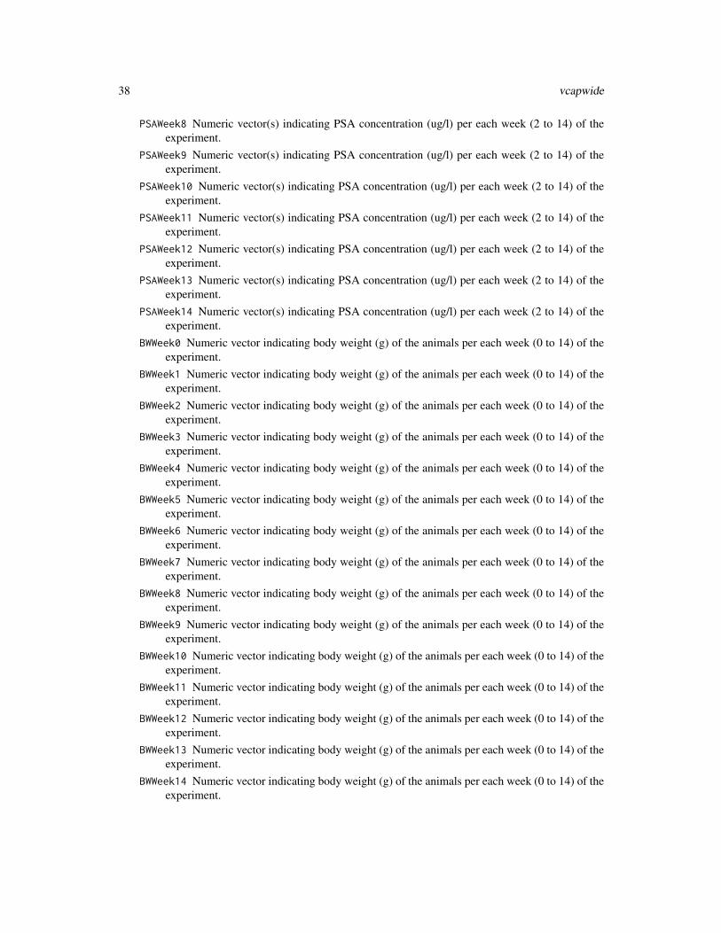
38 vcapwide








BWWeek0 Numeric vector indicating body weight (g) of the animals per each week (0 to 14) of theexperiment.















vcapwide 39

Details

The wide-format here presented the longitudinal measurements for PSA and Body Weight per eachcolumn. For modeling the PSA growth longitudinally e.g. using mixed-effects models, see thevcaplong dataset where the data has been readily transposed into the long-format.

Source



See Also

vcaplong

Examples

data(vcapwide)

str(vcapwide)head(vcapwide)

mixplot(vcapwide[,c("PSAWeek10", "PSAWeek14", "BWWeek10", "Group")], pch=16)anv <- aov(PSA ~ Group, data.frame(PSA = vcapwide[,"PSAWeek14"], Group = vcapwide[,"Group"]))summary(anv)TukeyHSD(anv)summary(aov(BW ~ Group, data.frame(BW = vcapwide[,"BWWeek14"], Group = vcapwide[,"Group"])))

Index

∗Topic aplothmap, 5hmap.annotate, 8hmap.key, 10

∗Topic clustermatch.bb, 13

∗Topic datasetsorxlong, 31orxwide, 33vcaplong, 35vcapwide, 37

∗Topic designmatch.allocate, 12match.bb, 13mem.powersimu, 25

∗Topic dplotextendsymrange, 4smartjitter, 34

∗Topic gamatch.ga, 16

∗Topic hplothmap, 5hmap.annotate, 8hmap.key, 10mixplot, 29

∗Topic manipmatch.dummy, 15match.mat2vec, 19match.vec2mat, 21mix.binary, 27mix.fun, 28

∗Topic memmem.powersimu, 25

∗Topic packagehamlet-package, 2

∗Topic powermem.powersimu, 25

∗Topic regressionmem.getcomp, 22

mem.plotran, 23mem.plotresid, 24

apply, 29

extendrange, 5extendsymrange, 4

hamlet (hamlet-package), 2hamlet-package, 2heatmap, 7, 10, 11hmap, 5, 10, 11hmap.annotate, 7, 8, 11hmap.key, 7, 10, 10

match.allocate, 12, 14, 16, 20, 21match.bb, 12, 13, 16, 19–21match.dummy, 12, 14, 15, 20, 21match.ga, 16match.mat2vec, 12, 14, 16, 19, 21match.vec2mat, 12, 14, 16, 20, 21mem.getcomp, 22, 23, 24, 27mem.plotran, 23, 23, 24mem.plotresid, 23, 24mem.powersimu, 25mix.binary, 27mix.fun, 28mixplot, 29

orxlong, 31orxwide, 33

smartjitter, 34

vcaplong, 35, 39vcapwide, 37

40

Package ‘hamlet’ - R · The package ’hamlet’ offers functions for optimal matching,...

Documents

Transcript of Package ‘hamlet’ - R · The package ’hamlet’ offers functions for optimal matching,...