Package ‘ForeCA’ - The Comprehensive R Archive Network · continuous_entropy 5 prior.probs...

Package ‘ForeCA’March 30, 2016

Type Package

Title Forecastable Component Analysis

Version 0.2.4

Date 2016-03-01

Author Georg M. Goerg <[email protected]>

Maintainer Georg M. Goerg <[email protected]>

URL http://www.gmge.org

Description Implementation of Forecastable Component Analysis ('ForeCA'),including main algorithms and auxiliary function (summary, plotting, etc.) toapply 'ForeCA' to multivariate time series data. 'ForeCA' is a novel dimensionreduction (DR) technique for temporally dependent signals. Contrary to otherpopular DR methods, such as 'PCA' or 'ICA', 'ForeCA' takes time dependencyexplicitly into account and searches for the most ''forecastable'' signal.The measure of forecastability is based on the Shannon entropy of the spectraldensity of the transformed signal.

Depends R (>= 3.0.0), ifultools (>= 2.0.0)

License GPL-2

Imports MASS, sapa, graphics, reshape2, utils

Suggests astsa, mgcv, nlme (>= 3.1-64), testthat (>= 0.9.0), rSFA,

RoxygenNote 5.0.1

NeedsCompilation no

Repository CRAN

Date/Publication 2016-03-30 08:14:22

R topics documented:ForeCA-package . . . . . . . . . . . . . . . . . . . . . . . . . . . . . . . . . . . . . . 2common-arguments . . . . . . . . . . . . . . . . . . . . . . . . . . . . . . . . . . . . . 3complete-controls . . . . . . . . . . . . . . . . . . . . . . . . . . . . . . . . . . . . . . 4continuous_entropy . . . . . . . . . . . . . . . . . . . . . . . . . . . . . . . . . . . . . 5

1

http://www.gmge.org

2 ForeCA-package

discrete_entropy . . . . . . . . . . . . . . . . . . . . . . . . . . . . . . . . . . . . . . . 7foreca . . . . . . . . . . . . . . . . . . . . . . . . . . . . . . . . . . . . . . . . . . . . 8foreca-utils . . . . . . . . . . . . . . . . . . . . . . . . . . . . . . . . . . . . . . . . . 11foreca.EM-aux . . . . . . . . . . . . . . . . . . . . . . . . . . . . . . . . . . . . . . . 12foreca.EM.one_weightvector . . . . . . . . . . . . . . . . . . . . . . . . . . . . . . . . 14foreca.one_weightvector-utils . . . . . . . . . . . . . . . . . . . . . . . . . . . . . . . . 16initialize_weightvector . . . . . . . . . . . . . . . . . . . . . . . . . . . . . . . . . . . 17mvspectrum . . . . . . . . . . . . . . . . . . . . . . . . . . . . . . . . . . . . . . . . . 18mvspectrum-utils . . . . . . . . . . . . . . . . . . . . . . . . . . . . . . . . . . . . . . 21mvspectrum2wcov . . . . . . . . . . . . . . . . . . . . . . . . . . . . . . . . . . . . . 22Omega . . . . . . . . . . . . . . . . . . . . . . . . . . . . . . . . . . . . . . . . . . . . 24quadratic_form . . . . . . . . . . . . . . . . . . . . . . . . . . . . . . . . . . . . . . . 26sfa . . . . . . . . . . . . . . . . . . . . . . . . . . . . . . . . . . . . . . . . . . . . . . 27spectral_entropy . . . . . . . . . . . . . . . . . . . . . . . . . . . . . . . . . . . . . . . 28whiten . . . . . . . . . . . . . . . . . . . . . . . . . . . . . . . . . . . . . . . . . . . . 30

Index 33

ForeCA-package Implementation of Forecastable Component Analysis (ForeCA)

Description

Forecastable Component Analysis (ForeCA) is a novel dimension reduction technique for multi-variate time series Xt. ForeCA finds a linar combination yt = Xtv that is easy to forecast. Themeasure of forecastability Ω(yt) (Omega) is based on the entropy of the spectral density fy(λ) ofyt: higher entropy means less forecastable, lower entropy is more forecastable.

The main function foreca runs ForeCA on a multivariate time series Xt.

Please consult the NEWS file for a list of changes to previous versions of this package.

Author(s)

Author and maintainer: Georg M. Goerg <[email protected]>

References

Goerg, G. M. (2013). “Forecastable Component Analysis”. Journal of Machine Learning Re-search (JMLR) W&CP 28 (2): 64-72, 2013. Available at jmlr.org/proceedings/papers/v28/goerg13.html.

Examples

XX <- ts(diff(log(EuStockMarkets)))Omega(XX)

plot(log10(lynx))Omega(log10(lynx))

jmlr.org/proceedings/papers/v28/goerg13.html


common-arguments 3

## Not run:ff <- foreca(XX, n.comp = 4)ffplot(ff)summary(ff)

## End(Not run)

common-arguments List of common arguments

Description

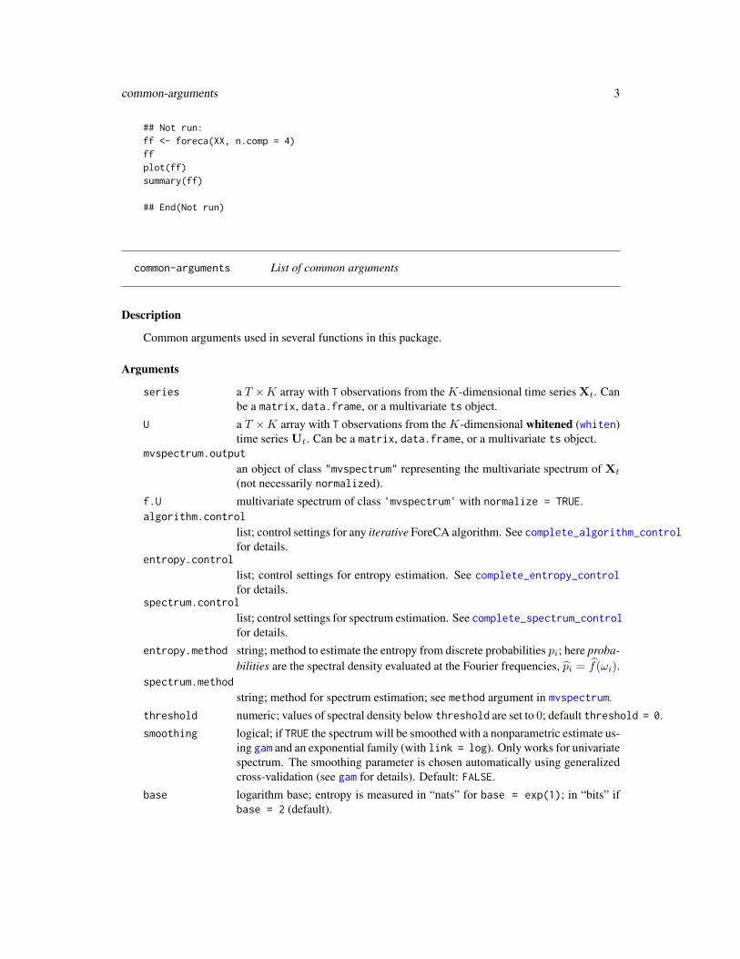
Common arguments used in several functions in this package.

Arguments

series a T ×K array with T observations from the K-dimensional time series Xt. Canbe a matrix, data.frame, or a multivariate ts object.

U a T ×K array with T observations from the K-dimensional whitened (whiten)time series Ut. Can be a matrix, data.frame, or a multivariate ts object.

mvspectrum.output

an object of class "mvspectrum" representing the multivariate spectrum of Xt

(not necessarily normalized).f.U multivariate spectrum of class 'mvspectrum' with normalize = TRUE.algorithm.control

list; control settings for any iterative ForeCA algorithm. See complete_algorithm_controlfor details.

entropy.control

list; control settings for entropy estimation. See complete_entropy_controlfor details.

spectrum.control

list; control settings for spectrum estimation. See complete_spectrum_controlfor details.

entropy.method string; method to estimate the entropy from discrete probabilities pi; here proba-bilities are the spectral density evaluated at the Fourier frequencies, pi = f(ωi).

spectrum.method

string; method for spectrum estimation; see method argument in mvspectrum.threshold numeric; values of spectral density below threshold are set to 0; default threshold = 0.smoothing logical; if TRUE the spectrum will be smoothed with a nonparametric estimate us-

ing gam and an exponential family (with link = log). Only works for univariatespectrum. The smoothing parameter is chosen automatically using generalizedcross-validation (see gam for details). Default: FALSE.

base logarithm base; entropy is measured in “nats” for base = exp(1); in “bits” ifbase = 2 (default).

4 complete-controls

complete-controls Completes several control settings

Description

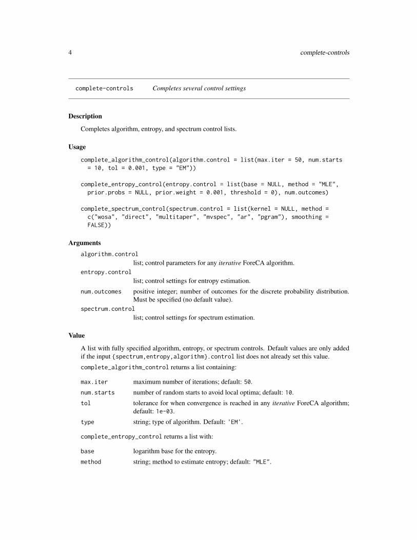
Completes algorithm, entropy, and spectrum control lists.

Usage

complete_algorithm_control(algorithm.control = list(max.iter = 50, num.starts= 10, tol = 0.001, type = "EM"))

complete_entropy_control(entropy.control = list(base = NULL, method = "MLE",prior.probs = NULL, prior.weight = 0.001, threshold = 0), num.outcomes)

complete_spectrum_control(spectrum.control = list(kernel = NULL, method =c("wosa", "direct", "multitaper", "mvspec", "ar", "pgram"), smoothing =FALSE))

Arguments

algorithm.control

list; control parameters for any iterative ForeCA algorithm.entropy.control

list; control settings for entropy estimation.

num.outcomes positive integer; number of outcomes for the discrete probability distribution.Must be specified (no default value).

spectrum.control

list; control settings for spectrum estimation.

Value

A list with fully specified algorithm, entropy, or spectrum controls. Default values are only addedif the input spectrum,entropy,algorithm.control list does not already set this value.

complete_algorithm_control returns a list containing:

max.iter maximum number of iterations; default: 50.

num.starts number of random starts to avoid local optima; default: 10.

tol tolerance for when convergence is reached in any iterative ForeCA algorithm;default: 1e-03.

type string; type of algorithm. Default: 'EM'.

complete_entropy_control returns a list with:

base logarithm base for the entropy.

method string; method to estimate entropy; default: "MLE".

continuous_entropy 5

prior.probs prior distribution; default: uniform rep(1 / num.outcomes, num.outcomes).

prior.weight weight of the prior distribution; default: 1e-3.

threshold non-negative float; set probabilities below threshold to zero; default: 0.

complete_spectrum_control returns a list containing:

kernel R function; function to weigh each Fourier frequency λ; default: NULL (no re-weighting).

method string; method to estimate the spectrum; default: 'wosa' if sapa is installed,'mvspec' if only astsa is installed, and 'pgram' if neither is installed.

smoothing logical; default: FALSE.

Available methods for spectrum estimation are (alphabetical order)

"ar" autoregressive spectrum fit via spec.ar; only for univariate time series.

"direct" raw periodogram using SDF.

"multitaper" tapering the periodogram using SDF.

"mvspec" smoothed estimate using mvspec; many tuning parameters are available – theycan be passed as additional arguments (...) to mvspectrum.

"pgram" uses mvpgram; is the same as the 'direct' method, but does not rely on the SDFpackage.

"wosa" Welch overlapping segment averaging (WOSA) using SDF.

Setting smoothing = TRUE will smooth the estimated spectrum (again); this option is only avail-able for univariate time series/spectra.

See Also

mvspectrum, discrete_entropy, continuous_entropy

continuous_entropy Shannon entropy for a continuous pdf

Description

Computes the Shannon entropyH(p) for a continuous probability density function (pdf) p(x) usingnumerical integration.

Usage

continuous_entropy(pdf, lower, upper, base = 2)

6 continuous_entropy

Arguments

pdf R function for the pdf p(x) of a RV X ∼ p(x). This function must be non-negative and integrate to 1 over the interval [lower, upper].

lower, upper lower and upper integration limit. pdf must integrate to 1 on this interval.


Details

The Shannon entropy of a continuous random variable (RV) X ∼ p(x) is defined as

H(p) = −∫ ∞−∞

p(x) log p(x)dx.

Contrary to discrete RVs, continuous RVs can have negative entropy (see Examples).

Value

scalar; entropy value (real).

Since continuous_entropy uses numerical integration (integrate()) convergence is not garantueed(even if integral in definition ofH(p) exists). Issues a warning if integrate() does not converge.

See Also

discrete_entropy

Examples

# entropy of U(a, b) = log(b - a). Thus not necessarily positive anymore, e.g.continuous_entropy(function(x) dunif(x, 0, 0.5), 0, 0.5) # log2(0.5)

# Same, but for U(-1, 1)my_density <- function(x)

dunif(x, -1, 1)continuous_entropy(my_density, -1, 1) # = log(upper - lower)

# a 'triangle' distributioncontinuous_entropy(function(x) x, 0, sqrt(2))

discrete_entropy 7

discrete_entropy Shannon entropy for discrete pmf

Description

Computes the Shannon entropy H(p) = −∑ni=1 pi log pi of a discrete RV X taking values in

x1, . . . , xn with probability mass function (pmf) P (X = xi) = pi with pi ≥ 0 for all i and∑ni=1 pi = 1.

Usage

discrete_entropy(probs, base = 2, method = c("MLE"), threshold = 0,prior.probs = rep(1/length(probs), length = length(probs)),prior.weight = 0)

Arguments

probs numeric; probabilities (empirical frequencies). Must be non-negative and addup to 1.


method string; method to estimate entropy; see Details below.

threshold numeric; frequencies below threshold are set to 0; default threshold = 0,i.e., no thresholding. If prior.weight > 0 then thresholding will be donebefore smoothing.

prior.probs optional; only used if prior.weight > 0. Add a prior probability distributionto probs. By default it uses a uniform distribution putting equal probability oneach outcome.

prior.weight numeric; how much weight does the prior distribution get in a mixture modelbetween data and prior distribution? Must be between 0 and 1. Default: 0 (noprior).

Details

discrete_entropy uses a plug-in estimator (method = "MLE"):

H(p) = −n∑i=1

pi log pi.

If prior.weight > 0, then it mixes the observed proportions pi with a prior distribution

pi ← (1− λ) · pi + λ · priori, i = 1, . . . , n,

where λ ∈ [0, 1] is the prior.weight parameter. By default the prior is a uniform distribution, i.e.,priori = 1

n for all i.

Note that this plugin estimator is biased. See References for an overview of alternative methods.

8 foreca

Value

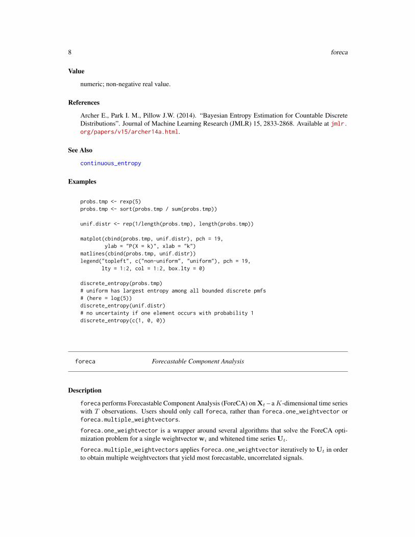
numeric; non-negative real value.

References

Archer E., Park I. M., Pillow J.W. (2014). “Bayesian Entropy Estimation for Countable DiscreteDistributions”. Journal of Machine Learning Research (JMLR) 15, 2833-2868. Available at jmlr.org/papers/v15/archer14a.html.

See Also

continuous_entropy

Examples

probs.tmp <- rexp(5)probs.tmp <- sort(probs.tmp / sum(probs.tmp))

unif.distr <- rep(1/length(probs.tmp), length(probs.tmp))

matplot(cbind(probs.tmp, unif.distr), pch = 19,ylab = "P(X = k)", xlab = "k")

matlines(cbind(probs.tmp, unif.distr))legend("topleft", c("non-uniform", "uniform"), pch = 19,

lty = 1:2, col = 1:2, box.lty = 0)

discrete_entropy(probs.tmp)# uniform has largest entropy among all bounded discrete pmfs# (here = log(5))discrete_entropy(unif.distr)# no uncertainty if one element occurs with probability 1discrete_entropy(c(1, 0, 0))

foreca Forecastable Component Analysis

Description

foreca performs Forecastable Component Analysis (ForeCA) on Xt – aK-dimensional time serieswith T observations. Users should only call foreca, rather than foreca.one_weightvector orforeca.multiple_weightvectors.

foreca.one_weightvector is a wrapper around several algorithms that solve the ForeCA opti-mization problem for a single weightvector wi and whitened time series Ut.

foreca.multiple_weightvectors applies foreca.one_weightvector iteratively to Ut in orderto obtain multiple weightvectors that yield most forecastable, uncorrelated signals.

jmlr.org/papers/v15/archer14a.html

jmlr.org/papers/v15/archer14a.html

foreca 9

Usage

foreca(series, n.comp = 2, algorithm.control = list(type = "EM"), ...)

foreca.one_weightvector(U, f.U = NULL, spectrum.control = list(),entropy.control = list(), algorithm.control = list(),keep.all.optima = FALSE, dewhitening = NULL, ...)

foreca.multiple_weightvectors(U, spectrum.control = list(),entropy.control = list(), algorithm.control = list(), n.comp = 2,plot = FALSE, dewhitening = NULL, ...)

Arguments


n.comp positive integer; number of components to be extracted. Default: 2.algorithm.control


... additional arguments passed to available ForeCA algorithms.


f.U multivariate spectrum of class 'mvspectrum' with normalize = TRUE.spectrum.control


entropy.control


keep.all.optima

logical; if TRUE, it keeps the optimal solutions of each random start. Default:FALSE (only returns the best solution).

dewhitening optional; if provided (returned by whiten) then it uses the dewhitening transfor-mation to obtain the original series Xt and it uses that vector (normalized) asthe initial weightvector which corresponds to the series Xt,i with larges Omega.

plot logical; if TRUE a plot of the current optimal solution w∗i will be shown andupdated for each iteration i = 1, ..., n.comp of any iterative algorithm. Default:FALSE.

Value

An object of class foreca, which is similar to the output from princomp, with the following com-ponents (amongst others):

• center: sample mean µX of each series,

• whitening: whitening matrix of size K ×K from whiten: Ut = (Xt − µX) · whitening;note that Xt is centered prior to the whitening transformation,

10 foreca

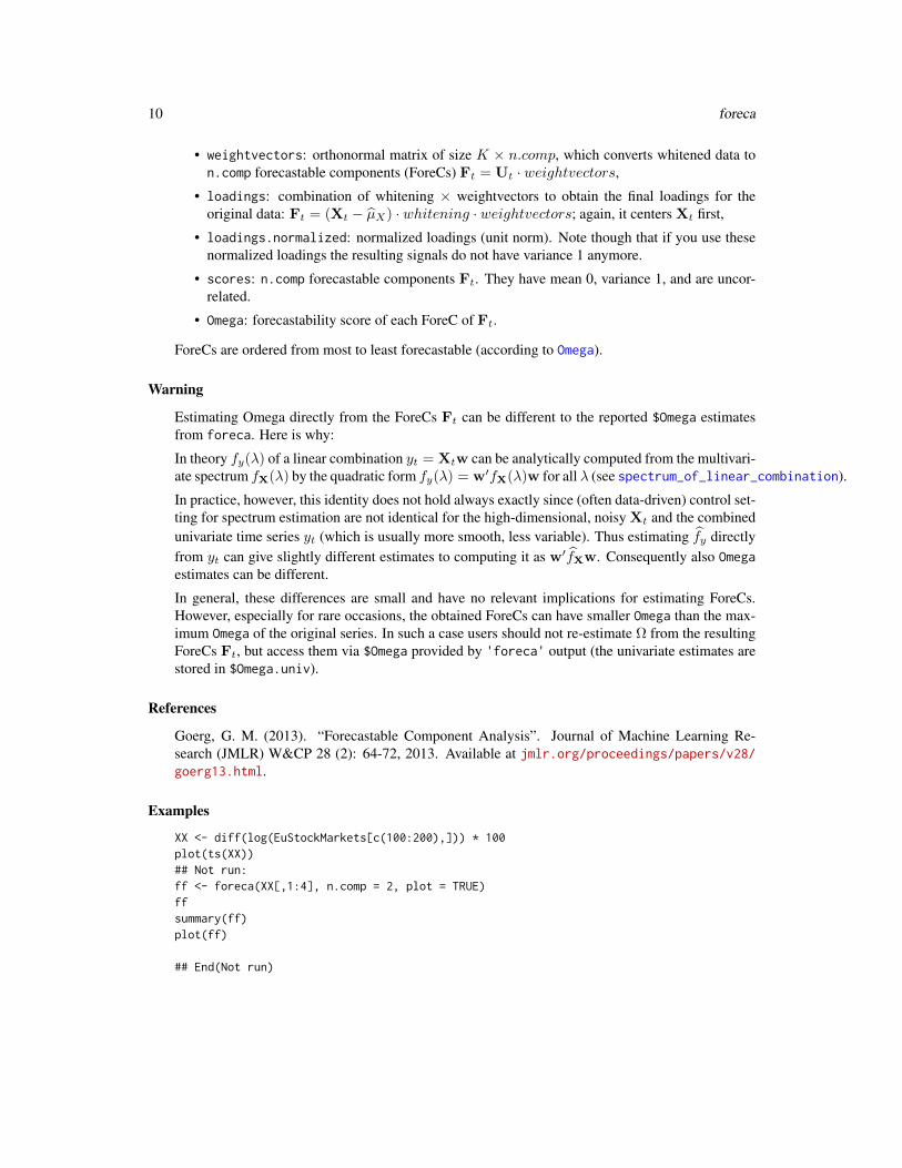
• weightvectors: orthonormal matrix of size K × n.comp, which converts whitened data ton.comp forecastable components (ForeCs) Ft = Ut · weightvectors,

• loadings: combination of whitening × weightvectors to obtain the final loadings for theoriginal data: Ft = (Xt − µX) · whitening · weightvectors; again, it centers Xt first,

• loadings.normalized: normalized loadings (unit norm). Note though that if you use thesenormalized loadings the resulting signals do not have variance 1 anymore.

• scores: n.comp forecastable components Ft. They have mean 0, variance 1, and are uncor-related.

• Omega: forecastability score of each ForeC of Ft.

ForeCs are ordered from most to least forecastable (according to Omega).

Warning

Estimating Omega directly from the ForeCs Ft can be different to the reported $Omega estimatesfrom foreca. Here is why:

In theory fy(λ) of a linear combination yt = Xtw can be analytically computed from the multivari-ate spectrum fX(λ) by the quadratic form fy(λ) = w′fX(λ)w for all λ (see spectrum_of_linear_combination).

In practice, however, this identity does not hold always exactly since (often data-driven) control set-ting for spectrum estimation are not identical for the high-dimensional, noisy Xt and the combinedunivariate time series yt (which is usually more smooth, less variable). Thus estimating fy directlyfrom yt can give slightly different estimates to computing it as w′fXw. Consequently also Omegaestimates can be different.

In general, these differences are small and have no relevant implications for estimating ForeCs.However, especially for rare occasions, the obtained ForeCs can have smaller Omega than the max-imum Omega of the original series. In such a case users should not re-estimate Ω from the resultingForeCs Ft, but access them via $Omega provided by 'foreca' output (the univariate estimates arestored in $Omega.univ).

References


Examples

XX <- diff(log(EuStockMarkets[c(100:200),])) * 100plot(ts(XX))## Not run:ff <- foreca(XX[,1:4], n.comp = 2, plot = TRUE)ffsummary(ff)plot(ff)

## End(Not run)



foreca-utils 11

PW <- whiten(XX)one.weight.em <- foreca.one_weightvector(U = PW$U,

dewhitening = PW$dewhitening,algorithm.control =

list(num.starts = 2,type = "EM"),

spectrum.control =list(method = 'wosa'))

plot(one.weight.em)

## Not run:

PW <- whiten(XX)ff <- foreca.multiple_weightvectors(PW$U, n.comp = 2,

dewhitening = PW$dewhitening)ffplot(ff$scores)

## End(Not run)

foreca-utils Plot, summary, and print methods for class ’foreca’

Description

A collection of S3 methods for estimated ForeCA results (class "foreca").

summary.foreca computes summary statistics.

print.foreca prints a human-readable summary in the console.

biplot.foreca shows a biplot of the ForeCA loadings (wrapper around biplot.princomp).

plot.foreca shows biplots, screeplots, and white noise tests.

Usage

## S3 method for class 'foreca'summary(object, lag = 10, alpha = 0.05, ...)

## S3 method for class 'foreca'print(x, ...)

## S3 method for class 'foreca'biplot(x, ...)

## S3 method for class 'foreca'plot(x, lag = 10, alpha = 0.05, ...)

12 foreca.EM-aux

Arguments

lag integer; how many lags to test in Box.test; default: 10.

alpha significance level for testing white noise in Box.test; default: 0.05.

... additional arguments passed to biplot.princomp, biplot.default, plot, orsummary.

x, object an object of class "foreca".

Examples

# see examples in 'foreca'

foreca.EM-aux ForeCA EM auxiliary functions

Description

foreca.EM.one_weightvector relies on several auxiliary functions:

foreca.EM.E_step computes the spectral density of yt = Utw given the weightvector w and thenormalized spectrum estimate fU. A wrapper around spectrum_of_linear_combination.

foreca.EM.M_step computes the minimizing eigenvector (→ wi+1) of the weighted covariancematrix, where the weights equal the negative logarithm of the spectral density at the current wi.

foreca.EM.E_and_M_step is a wrapper around foreca.EM.E_step followed by foreca.EM.M_step.

foreca.EM.h evaluates (an upper bound of) the entropy of the spectral density as a function of wi

(or wi+1). This is the objective funcion that should be minimized.

Usage

foreca.EM.E_step(f.U, weightvector)

foreca.EM.M_step(f.U, f.current, minimize = TRUE, entropy.control = list())

foreca.EM.E_and_M_step(weightvector, f.U, minimize = TRUE,entropy.control = list())

foreca.EM.h(weightvector.new, f.U, weightvector.current = weightvector.new,f.current = NULL, entropy.control = list(), return.negative = FALSE)

Arguments

f.U multivariate spectrum of class 'mvspectrum' with normalize = TRUE.

weightvector numeric; weights w for yt = Utw. Must have unit norm in `2.

f.current numeric; spectral density estimate of yt = Utw for the current estimate wi

(required for foreca.EM.M_step; optional for foreca.EM.h).

foreca.EM-aux 13

minimize logical; if TRUE (default) it returns the eigenvector corresponding to the smallesteigenvalue; otherwise to the largest eigenvalue.

entropy.control


weightvector.new

weightvector wi+1 of the new iteration (i+1).weightvector.current

weightvector wi of the current iteration (i).return.negative

logical; if TRUE it returns the negative spectral entropy. This is useful whenmaximizing forecastibility which is equivalent (up to an additive constant) tomaximizing negative entropy. Default: FALSE.

Value

foreca.EM.E_step returns the normalized univariate spectral density (normalized such that its sumequals 0.5).

foreca.EM.M_step returns a list with three elements:

• matrix: weighted covariance matrix, where the weights are the negative log of the spectraldensity. If density is estimated by discrete probabilities, then this matrix is positive semi-definite, since − log(p) ≥ 0 for p ∈ [0, 1]. See weightvector2entropy_wcov.

• vector: minimizing (or maximizing if minimize = FALSE) eigenvector of matrix,

• value: corresponding eigenvalue.

Contrary to foreca.EM.M_step, foreca.EM.E_and_M_step only returns the optimal weightvectoras a numeric.

foreca.EM.h returns non-negative real value (see References for details):

• entropy, if weightvector.new = weightvector.current,

• an upper bound of that entropy for weightvector.new, otherwise.

See Also

weightvector2entropy_wcov

Examples

XX <- diff(log(EuStockMarkets)) * 100UU <- whiten(XX)$Uff <- mvspectrum(UU, 'wosa', normalize = TRUE)

ww0 <- initialize_weightvector(num.series = ncol(XX), method = 'rnorm')

f.ww0 <- foreca.EM.E_step(ff, ww0)plot(f.ww0, type = "l")

one.step <- foreca.EM.M_step(ff, f.ww0,

14 foreca.EM.one_weightvector

entropy.control = list(prior.weight = 0.1))image(one.step$matrix)## Not run:requireNamespace(LICORS)# if you have the 'LICORS' package useLICORS::image2(one.step$matrix)

## End(Not run)ww1 <- one.step$vectorf.ww1 <- foreca.EM.E_step(ff, ww1)

layout(matrix(1:2, ncol = 2))matplot(seq(0, pi, length = length(f.ww0)), cbind(f.ww0, f.ww1),

type = "l", lwd =2, xlab = "omega_j", ylab = "f(omega_j)")plot(f.ww0, f.ww1, pch = ".", cex = 3, xlab = "iteration 0",

ylab = "iteration 1", main = "Spectral density")abline(0, 1, col = 'blue', lty = 2, lwd = 2)

Omega(mvspectrum.output = f.ww0) # startOmega(mvspectrum.output = f.ww1) # improved after one iteration

ww0 <- initialize_weightvector(NULL, ff, method = "rnorm")ww1 <- foreca.EM.E_and_M_step(ww0, ff)ww0ww1barplot(rbind(ww0, ww1), beside = TRUE)abline(h = 0, col = "blue", lty = 2)

foreca.EM.h(ww0, ff) # iteration 0foreca.EM.h(ww1, ff, ww0) # min eigenvalue inequalityforeca.EM.h(ww1, ff) # KL divergence inequalityone.step$value

# by definition of Omega, they should equal 1 (modulo rounding errors)Omega(mvspectrum.output = f.ww0) / 100 + foreca.EM.h(ww0, ff)Omega(mvspectrum.output = f.ww1) / 100 + foreca.EM.h(ww1, ff)

foreca.EM.one_weightvector

EM-like algorithm to estimate optimal ForeCA transformation

Description

foreca.EM.one_weightvector finds the optimal weightvector w∗ that gives the most forecastablesignal y∗t = Utw

∗ using an EM-like algorithm (see References).

foreca.EM.one_weightvector 15

Usage

foreca.EM.one_weightvector(U, f.U = NULL, spectrum.control = list(),entropy.control = list(), algorithm.control = list(),init.weightvector = initialize_weightvector(num.series = ncol(U), method ="rnorm"), ...)

Arguments


f.U multivariate spectrum of class 'mvspectrum' with normalize = TRUE.spectrum.control


entropy.control


algorithm.control


init.weightvector

numeric; starting point w0 for several iterative algorithms. By default it uses a(normalized) random vector from a standard Normal distribution (see initialize_weightvector).

... other arguments passed to mvspectrum

Value

A list with useful quantities like the optimal weighvector, the corresponding signal, and its fore-castability.

References


See Also

foreca.one_weightvector, foreca.EM-aux

Examples

## Not run:XX <- diff(log(EuStockMarkets)[100:200,]) * 100one.weight <- foreca.EM.one_weightvector(whiten(XX)$U,

spectrum.control =list(method = "wosa"))

## End(Not run)



16 foreca.one_weightvector-utils

foreca.one_weightvector-utils

Plot, summary, and print methods for class ’foreca.one_weightvector’

Description

S3 methods for the one weightvector optimization in ForeCA (class "foreca.one_weightvector").

summary.foreca.one_weightvector computes summary statistics.

plot.foreca.one_weightvector shows the results of an (iterative) algorithm that obtained thei-th optimal a weightvector w∗i . It shows trace plots of the objective function and the weightvector,and a time series plot of the transformed signal y∗t along with its spectral density estimate fy(ωj).

Usage

## S3 method for class 'foreca.one_weightvector'summary(object, lag = 10, alpha = 0.05,...)

## S3 method for class 'foreca.one_weightvector'plot(x, main = "", cex.lab = 1.1, ...)

Arguments

lag integer; how many lags to test in Box.test; default: 10.

alpha significance level for testing white noise in Box.test; default: 0.05.

... additional arguments passed to plot, or summary.

x, object an object of class "foreca.one_weightvector".

main an overall title for the plot: see title.

cex.lab size of the axes labels.

Examples

# see examples in 'foreca.one_weightvector'

initialize_weightvector 17

initialize_weightvector

Initialize weightvector for iterative ForeCA algorithms

Description

initialize_weightvector returns a unit norm (in `2) vector w0 ∈ RK that can be used as thestarting point for any iterative ForeCA algorithm, e.g., foreca.EM.one_weightvector. Severalquickly computable heuristics are available via the method argument.

Usage

initialize_weightvector(U = NULL, f.U = NULL, num.series = ncol(U),method = c("rnorm", "max", "SFA", "PCA", "rcauchy", "runif", "SFA.slow","SFA.fast", "PCA.large", "PCA.small"), seed = sample(1e+06, 1), ...)

Arguments



num.series positive integer; number of time seriesK (determines the length of the weightvec-tor). If num.series = 1 it simply returns a 1 × 1 array equal to 1.

method string; which heuristics should be used to generate a good starting w0? Default:"rnorm"; see Details.

seed non-negative integer; seed for random initialization which will be returned forreproducibility. By default it sets a random seed.

... additional arguments

Details

The method argument specifies the heuristics that is used to get a good starting vector w0:

• "max" vector with all 0s, but a 1 at the position of the maximum forecastable series in U.

• "rcauchy" random start using rcauchy(k).

• "rnorm" random start using rnorm(k, 0, 1).

• "runif" random start using runif(k, -1, 1).

• "PCA.large" first eigenvector of PCA (largest variance signal).

• "PCA.small" last eigenvector of PCA (smallest variance signal).

• "PCA" checks both small and large, and chooses the one with higher forecastability as com-puted by Omega..

• "SFA.fast" last eigenvector of SFA (fastest signal).

• "SFA.slow" first eigenvector of SFA (slowest signal).

18 mvspectrum

• "SFA" checks both slow and fast, and chooses the one with higher forecastability as computedby Omega.

Each vector has length K and is automatically normalized to have unit norm in `2.

For the 'SFA*' methods see sfa. Note that maximizing (or minimizing) the lag 1 auto-correlationdoes not necessarily yield the most forecastable signal, but it’s a good start.

Value

numeric; a vector of length K with unit norm in `2.

Examples

XX <- diff(log(EuStockMarkets))## Not run:initialize_weightvector(U = XX, method = "SFA")

## End(Not run)initialize_weightvector(num.series = ncol(XX), method = "rnorm")

mvspectrum Estimates spectrum of multivariate time series

Description

The spectrum of a multivariate time series is a matrix-valued function of the frequency λ ∈ [−π, π],which is symmetric/Hermitian around λ = 0.

mvspectrum estimates it and returns a 3D array of dimension num.freqs × K × K. Since thespectrum is symmetric/Hermitian around λ = 0 it is sufficient to store only positive frequencies. Inthe implementation in this package we thus usually consider only positive frequencies (omitting 0);num.freqs refers to the number of positive frequencies only.

normalize_mvspectrum normalizes the spectrum such that it adds up to 0.5 over all positive fre-quencies (by symmetry it will add up to 1 over the whole range – thus the name normalize).

For a K-dimensional time series it adds up to a Hermitian K ×K matrix with 0.5 in the diagonaland imaginary elements (real parts equal to 0) in the off-diagonal. Since it is Hermitian the mvspec-trum will add up to the identity matrix over the whole range of frequencies, since the off-diagonalelements are purely imaginary (real part equals 0) and thus add up to 0.

check_mvspectrum_normalized checks if the spectrum is normalized (see normalize_mvspectrumfor the requirements).

mvpgram computes the multivariate periodogram estimate using bare-bone multivariate fft (mvfft).Please use mvspectrum(..., method = 'pgram') instead of mvpgram directly.

This function is merely included to have one method that does not require the astsa nor the sapaR packages. However, it is strongly encouraged to install either one of them to get (much) betterestimates. See Details.

get_spectrum_from_mvspectrum extracts the spectrum of one time series from an "mvspectrum"object by taking the i-th diagonal entry for each frequency.

mvspectrum 19

spectrum_of_linear_combination computes the spectrum of the linear combination yt = Xtβof K time series Xt. This can be efficiently computed by the quadratic form

fy(λ) = β′fX(λ)β ≥ 0,

for each λ. This holds for any β (even β = 0 – not only for ||β||2 = 1. For β = ei (the i-th basisvector) this is equivalent to get_spectrum_from_mvspectrum(..., which = i).

Usage

mvspectrum(series, method = c("pgram", "multitaper", "direct", "wosa","mvspec", "ar"), normalize = FALSE, smoothing = FALSE, ...)

normalize_mvspectrum(mvspectrum.output)

check_mvspectrum_normalized(f.U, check.attribute.only = TRUE)

mvpgram(series)

get_spectrum_from_mvspectrum(mvspectrum.output,which = seq_len(dim(mvspectrum.output)[2]))

spectrum_of_linear_combination(mvspectrum.output, beta)

Arguments


method string; method for spectrum estimation; see method argument in SDF (in thesapa package); use "mvspec" to use mvspec (astsa package); or use "pgram" touse spec.pgram.

normalize logical; if TRUE the spectrum will be normalized (see Value below for details).smoothing logical; if TRUE the spectrum will be smoothed with a nonparametric estimate us-

ing gam and an exponential family (with link = log). Only works for univariatespectrum. The smoothing parameter is chosen automatically using generalizedcross-validation (see gam for details). Default: FALSE.

mvspectrum.output


(not necessarily normalized).f.U multivariate spectrum of class 'mvspectrum' with normalize = TRUE.check.attribute.only

logical; if TRUE it checks the attribute only. This is much faster (it just needsto look up one attribute value), but it might not surface silent bugs. For sakeof performance the package uses the attribute version by default. However, fortesting/debugging the full computational version can be used.

which integer(s); the spectrum of which series whould be extracted. By default, itreturns all univariate spectra as a matrix (frequencies in rows).

beta numeric; vector β that defines the linear combination.... additional arguments passed to SDF or mvspec (e.g., taper)

20 mvspectrum

Details

For an orthonormal time series Ut the raw periodogram adds up to IK over all (negative and pos-itive) frequencies. Since we only consider positive frequencies, the normalized multivariate spec-trum should add up to 0.5 · IK plus a Hermitian imaginary matrix (which will add up to zero whencombined with its symmetric counterpart.) As we often use non-parametric smoothing for lessvariance, the spectrum estimates do not satisfy this identity exactly. normalize_mvspectrum thusadjust the estimates so they satisfy it again exactly.

mvpgram has no options for improving spectrum estimation whatsoever. It thus yields very noisy(in fact, inconsistent) estimates of the multivariate spectrum fX(λ). If you want to obtain betterestimates then please use other methods in mvspectrum (this is highly recommended to obtainmore reasonable/stable estimates).

Value

mvspectrum returns a 3D array of dimension num.freqs×K ×K, where

• num.freqs is the number of frequencies

• K is the number of series (columns in series).

Note that it also has an attribute "normalized" which is FALSE if normalize = FALSE; otherwiseTRUE. See normalize_mvspectrum for details.

normalize_mvspectrum returns a normalized spectrum over positive frequencies, which:

univariate: adds up to 0.5,

multivariate: adds up to Hermitian K ×K matrix with 0.5 in the diagonal and purely imaginaryelements in the off-diagonal.

check_mvspectrum_normalized throws an error if spectrum is not normalized correctly.

get_spectrum_from_mvspectrum returns either a matrix of all univariate spectra, or one singlecolumn (if which is specified.)

spectrum_of_linear_combination returns a vector with length equal to the number of rows ofmvspectrum.output.

References

See References in spectrum, SDF, mvspec.

Examples

set.seed(1)XX <- cbind(rnorm(100), arima.sim(n = 100, list(ar = 0.9)))ss3d <- mvspectrum(XX)dim(ss3d)

ss3d[2,,] # at omega_1; in general complex-valued, but Hermitianidentical(ss3d[2,,], Conj(t(ss3d[2,,]))) # is Hermitian

ss <- mvspectrum(XX[, 1], smoothing = TRUE)

mvspectrum-utils 21

## Not run:mvspectrum(XX, normalize = TRUE)

## End(Not run)ss <- mvspectrum(whiten(XX)$U, normalize = TRUE)

xx <- scale(rnorm(100), center = TRUE, scale = FALSE)var(xx)sum(mvspectrum(xx, normalize = FALSE, method = "direct")) * 2sum(mvspectrum(xx, normalize = FALSE, method = "wosa")) * 2

xx <- scale(rnorm(100), center = TRUE, scale = FALSE)ss <- mvspectrum(xx)ss.n <- normalize_mvspectrum(ss)sum(ss.n)# multivariateUU <- whiten(matrix(rnorm(40), ncol = 2))$US.U <- mvspectrum(UU, method = "wosa")mvspectrum2wcov(normalize_mvspectrum(S.U))

XX <- matrix(rnorm(1000), ncol = 2)SS <- mvspectrum(XX, "direct")ss1 <- mvspectrum(XX[, 1], "direct")

SS.1 <- get_spectrum_from_mvspectrum(SS, 1)plot.default(ss1, SS.1)abline(0, 1, lty = 2, col = "blue")

XX <- matrix(arima.sim(n = 1000, list(ar = 0.9)), ncol = 4)beta.tmp <- rbind(1, -1, 2, 0)yy <- XX %*% beta.tmp

SS <- mvspectrum(XX, "wosa")ss.yy.comb <- spectrum_of_linear_combination(SS, beta.tmp)ss.yy <- mvspectrum(yy, "wosa")

plot(ss.yy, log = TRUE) # using plot.mvspectrum()lines(ss.yy.comb, col = "red", lty = 1, lwd = 2)

mvspectrum-utils S3 methods for class ’mvspectrum’

Description

S3 methods for multivariate spectrum estimation.

plot.mvspectrum plots all univariate spectra. Analogouos to spectrum when plot = TRUE.

22 mvspectrum2wcov

Usage

## S3 method for class 'mvspectrum'plot(x, log = TRUE, ...)

Arguments

x an object of class "foreca.one_weightvector".

log logical; if TRUE (default), it plots the spectra on log-scale.

... additional arguments passed to matplot.

See Also

get_spectrum_from_mvspectrum

Examples

# see examples in 'mvspectrum'

SS <- mvspectrum(diff(log(EuStockMarkets)) * 100,spectrum.control = list(method = "multitaper"))

plot(SS, log = FALSE)

mvspectrum2wcov Compute (weighted) covariance matrix from frequency spectrum

Description

mvspectrum2wcov computes a (weighted) covariance matrix estimate from the frequency spectrum(see Details).

weightvector2entropy_wcov computes the weighted covariance matrix using the negative en-tropy of the univariate spectrum (given the weightvector) as kernel weights. This matrix is theobjective matrix for many foreca.* algorithms.

Usage

mvspectrum2wcov(mvspectrum.output, kernel.weights = 1)

weightvector2entropy_wcov(weightvector = NULL, f.U, f.current = NULL,entropy.control = list())

mvspectrum2wcov 23

Arguments

mvspectrum.output


(not necessarily normalized).

kernel.weights numeric; weights for each frequency. By default uses weights that average outto 1.

weightvector numeric; weights w for yt = Utw. Must have unit norm in `2.


f.current numeric; spectral density estimate of yt = Utw for the current estimate wi

(required for foreca.EM.M_step; optional for foreca.EM.h).entropy.control


Details

The covariance matrix of a multivariate time series satisfies the identity

ΣX ≡∫ π

−πSX(λ)dλ.

A generalized covariance matrix estimate can thus be obtained using a weighted average

ΣX =

∫ π

−πK(λ)SX(λ)dλ,

where K(λ) is a kernel symmetric around 0 which averages out to 1 over the interval [−π, π], i.e.,12π

∫ π−πK(λ)dλ = 1. This allows one to remove or amplify specific frequencies in the covariance

matrix estimation.

For ForeCA mvspectrum2wcov is especially important as we use

K(λ) = − log fy(λ),

as the weights (their average is not 1!). This particular kernel weight is implemented as a wrapperin weightvector2entropy_wcov.

Value

A symmetric n× n matrix.

If kernel.weights ≥ 0, then it is positive semi-definite; otherwise, it is symmetric but not neces-sarily positive semi-definite.

See Also

mvspectrum

24 Omega

Examples

nn <- 50YY <- cbind(rnorm(nn), arima.sim(n = nn, list(ar = 0.9)), rnorm(nn))XX <- YY %*% matrix(rnorm(9), ncol = 3) # random mixXX <- scale(XX, scale = FALSE, center = TRUE)

# sample estimate of covariance matrixSigma.hat <- cov(XX)dimnames(Sigma.hat) <- NULL

# using the frequency spectrumSS <- mvspectrum(XX, "wosa")Sigma.hat.freq <- mvspectrum2wcov(SS)

layout(matrix(1:4, ncol = 2))par(mar = c(2, 2, 1, 1))plot(c(Sigma.hat/Sigma.hat.freq))abline(h = 1)

image(Sigma.hat)image(Sigma.hat.freq)image(Sigma.hat / Sigma.hat.freq)

# examples for entropy wcovXX <- diff(log(EuStockMarkets)) * 100UU <- whiten(XX)$Uff <- mvspectrum(UU, 'wosa', normalize = TRUE)

ww0 <- initialize_weightvector(num.series = ncol(XX), method = 'rnorm')

weightvector2entropy_wcov(ww0, ff,entropy.control =

list(prior.weight = 0.1))

Omega Estimate forecastability of a time series

Description

An estimator for the forecastability Ω(xt) of a univariate time series xt. Currently it uses a discreteplug-in estimator given the empirical spectrum (periodogram).

Usage

Omega(series = NULL, spectrum.control = list(), entropy.control = list(),mvspectrum.output = NULL)

Omega 25

Arguments

series a univariate time series; if it is multivariate, then Omega works component-wise(i.e., same as apply(series, 2, Omega)).

spectrum.control


entropy.control


mvspectrum.output


(not necessarily normalized).

Details

The forecastability of a stationary process xt is defined as (see References)

Ω(xt) = 1−−∫ π−π fx(λ) log fx(λ)dλ

log 2π∈ [0, 1]

where fx(λ) is the normalized spectral density of xt. In particular∫ π−π fx(λ)dλ = 1.

For white noise εt forecastability Ω(εt) = 0; for a sum of sinusoids it equals 100 %. However,empirically it reaches 100% only if the estimated spectrum has exactly one peak at some ωj andf(ωk) = 0 for all k 6= j.

In practice, a time series of length T has T Fourier frequencies which represent a discrete probabilitydistribution. Hence entropy of fx(λ) must be normalized by log T , not by log 2π.

Also we can use several smoothing techniques to obtain a less variance estimate of fx(λ).

Value

A real-value between 0 and 100 (%). 0 means not forecastable (white noise); 100 means perfectlyforecastable (a sinusoid).

References


See Also

spectral_entropy, discrete_entropy, continuous_entropy



26 quadratic_form

Examples

nn <- 100eps <- rnorm(nn) # white noise has Omega() = 0 in theoryOmega(eps, spectrum.control = list(method = "direct"))# smoothing makes it closer to 0Omega(eps, spectrum.control = list(method = "wosa"))

xx <- sin(seq_len(nn) * pi / 10)Omega(xx, spectrum.control = list(method = "direct"))Omega(xx, entropy.control = list(threshold = 1/40))Omega(xx, spectrum.control = list(method = "wosa"),

entropy.control = list(threshold = 1/20))

# an AR(1) with phi = 0.5yy <- arima.sim(n = nn, model = list(ar = 0.5))Omega(yy, spectrum.control = list(method = "wosa"))

# an AR(1) with phi = 0.9 is more forecastableyy <- arima.sim(n = nn, model = list(ar = 0.9))Omega(yy, spectrum.control = list(method = "wosa"))

quadratic_form Computes quadratic form x’ A x

Description

quadratic_form computes the quadratic form x′Ax for an n× n matrix A and an n-dimensionalvector x, i.e., a wrapper for t(x) %*% A %*% x.

fill_symmetric and quadratic_form work with real and complex valued matrices/vectors.

fill_hermitian fills up the lower triangular part (NA) of an upper triangular matrix to its Hermitian(symmetric if real matrix) version, such that it satisfies A = A′, where z is the complex conjugateof z. If the matrix is real-valued this makes it simply symmetric.

Note that the input matrix must have a real-valued diagonal and NAs in the lower triangular part.

Usage

quadratic_form(mat, vec)

fill_hermitian(mat)

Arguments

mat numeric; n× n matrix (real or complex).

vec numeric; n× 1 vector (real or complex).

sfa 27

Value

A real/complex value x′Ax.

Examples

set.seed(1)AA <- matrix(1:4, ncol = 2)bb <- matrix(rnorm(2))t(bb) %*% AA %*% bbquadratic_form(AA, bb)

AA <- matrix(1:16, ncol = 4)AA[lower.tri(AA)] <- NAAA

fill_hermitian(AA)

sfa Slow Feature Analysis

Description

sfa performs Slow Feature Analysis (SFA) on a K-dimensional time series with T observations.

Important: This implementation of SFA is just the most basic version; it is merely included herefor convenience in initialize_weightvector. If you want to use SFA in R please use the rSFApackage, which has many more advanced and efficient implementations of SFA. sfa() here corre-sponds to sfa1 in the rSFA package.

Usage

sfa(series, ...)

Arguments


... additional arguments

Details

Slow Feature Analysis (SFA) finds slow signals (see References below), and can be quickly (andanalytically) computed solving a generalized eigen-value problem. For ForeCA it is important toknow that SFA is equivalent to finding the signal with largest lag 1 autocorrelation.

The disadvantage of SFA for forecasting is that, e.g., white noise (WN) is ranked higher than anAR(1) with negative autocorrelation coefficient ρ1 < 0. While it is true that WN is slower, it is not

28 spectral_entropy

more forecastable. Thus we are also interested in the fastest signal, i.e., the last eigenvector. The soobtained fastest signal corresponds to minimizing the lag 1 auto-correlation (possibly ρ1 < 0).

Note though that maximizing (or minimizing) the lag 1 auto-correlation does not necessarily yieldthe most forecastable signal (as measured by Omega), but it is a good start.

Value

An object of class sfa which inherits methods from princomp. Signals are ordered from slowest tofastest.

References

Laurenz Wiskott and Terrence J. Sejnowski (2002). “Slow Feature Analysis: Unsupervised Learn-ing of Invariances”, Neural Computation 14:4, 715-770.

See Also

initialize_weightvector

Examples

XX <- diff(log(EuStockMarkets[-c(1:100),])) * 100plot(ts(XX))ss <- sfa(XX[,1:4])

summary(ss)plot(ss)plot(ts(ss$scores))apply(ss$scores, 2, function(x) acf(x, plot = FALSE)$acf[2])biplot(ss)

spectral_entropy Estimates spectral entropy of a time series

Description

Estimates spectral entropy from a univariate (or multivariate) normalized spectral density.

Usage

spectral_entropy(series = NULL, spectrum.control = list(),entropy.control = list(), mvspectrum.output = NULL, ...)

spectral_entropy 29

Arguments

series univariate time series of length T . In the rare case that users want to call this fora multivariate time series, note that the estimated spectrum is in general notnormalized for the computation. Only if the original data is whitened, then it isnormalized.

spectrum.control


entropy.control


mvspectrum.output

optional; one can directly provide an estimate of the spectrum of series. Usu-ally the output of mvspectrum.

... additional arguments passed to mvspectrum.

Details

The spectral entropy equals the Shannon entropy of the spectral density fx(λ) of a stationary pro-cess xt:

Hs(xt) = −∫ π

−πfx(λ) log fx(λ)dλ,

where the density is normalized such that∫ π−π fx(λ)dλ = 1. An estimate of f(λ) can be obtained

by the (smoothed) periodogram (see mvspectrum); thus using discrete, and not continuous entropy.

Value

A non-negative real value for the spectral entropy Hs(xt).

References

Jerry D. Gibson and Jaewoo Jung (2006). “The Interpretation of Spectral Entropy Based Upon RateDistortion Functions”. IEEE International Symposium on Information Theory, pp. 277-281.

L. L. Campbell, “Minimum coefficient rate for stationary random processes”, Information and Con-trol, vol. 3, no. 4, pp. 360 - 371, 1960.

See Also

Omega, discrete_entropy

Examples

set.seed(1)eps <- rnorm(100)spectral_entropy(eps)

phi.v <- seq(-0.95, 0.95, by = 0.1)

30 whiten

kMethods <- c("wosa", "multitaper", "direct", "pgram")SE <- matrix(NA, ncol = length(kMethods), nrow = length(phi.v))for (ii in seq_along(phi.v))

xx.tmp <- arima.sim(n = 200, list(ar = phi.v[ii]))for (mm in seq_along(kMethods)) SE[ii, mm] <- spectral_entropy(xx.tmp, spectrum.control =

list(method = kMethods[mm]))

matplot(phi.v, SE, type = "l", col = seq_along(kMethods))legend("bottom", kMethods, lty = seq_along(kMethods),

col = seq_along(kMethods))

# AR vs MASE.arma <- matrix(NA, ncol = 2, nrow = length(phi.v))SE.arma[, 1] <- SE[, 2]

for (ii in seq_along(phi.v))yy.temp <- arima.sim(n = 1000, list(ma = phi.v[ii]))SE.arma[ii, 2] <-spectral_entropy(yy.temp, spectrum.control = list(method = "multitaper"))

matplot(phi.v, SE.arma, type = "l", col = 1:2, xlab = "parameter (phi or theta)",ylab = "Spectral entropy")

abline(v = 0, col = "blue", lty = 3)legend("bottom", c("AR(1)", "MA(1)"), lty = 1:2, col = 1:2)

whiten whitens multivariate data

Description

whiten transforms a multivariate K-dimensional signal X with mean µX and covariance matrixΣX to a whitened signal U with mean 0 and ΣU = IK . Thus it centers the signal and makes itcontemporaneously uncorrelated. See Details.

check_whitened checks if data has been whitened; i.e., if it has zero mean, unit variance, and isuncorrelated.

sqrt_matrix computes the square root B of a square matrix A. The matrix B satisfies BB = A.

Usage

whiten(data)

check_whitened(data, check.attribute.only = TRUE)

sqrt_matrix(mat, return.sqrt.only = TRUE, symmetric = FALSE)

whiten 31

Arguments

data n×K array representing n observations of K variables.check.attribute.only

logical; if TRUE it checks the attribute only. This is much faster (it just needsto look up one attribute value), but it might not surface silent bugs. For sakeof performance the package uses the attribute version by default. However, fortesting/debugging the full computational version can be used.

mat a square K ×K matrix.return.sqrt.only

logical; if TRUE (default) it returns only the square root matrix; if FALSE it returnsother auxiliary results (eigenvectors and eigenvalues, and inverse of the squareroot matrix).

symmetric logical; if TRUE the eigen-solver assumes that the matrix is symmetric (whichmakes it much faster). This is in particular useful for a covariance matrix (whichis used in whiten). Default: FALSE.

Details

whiten uses zero component analysis (ZCA) (aka zero-phase whitening filters) to whiten the data;i.e., it uses the inverse square root of the covariance matrix of X (see sqrt_matrix) as the whiteningtransformation. This means that on top of PCA, the uncorrelated principal components are back-transformed to the original space using the transpose of the eigenvectors. The advantage is that thismakes them comparable to the original X. See References for details.

The square root of a quadratic n× n matrix A can be computed by using the eigen-decompositionof A

A = VΛV′,

where Λ is an n × n matrix with the eigenvalues λ1, . . . , λn in the diagonal. The square root issimply B = VΛ1/2V′ where Λ1/2 = diag(λ

1/21 , . . . , λ

1/2n ).

Similarly, the inverse square root is defined as A−1/2 = VΛ−1/2V′, where Λ−1/2 = diag(λ−1/21 , . . . , λ

−1/2n )

(provided that λi 6= 0).

Value

whiten returns a list with the whitened data, the transformation, and other useful quantities.

check_whitened throws an error if the input is not whitened, and returns (invisibly) the data withan attribute 'whitened' equal to TRUE. This allows to simply update data to have the attribute andthus only check it once on the actual data (slow) but then use the attribute lookup (fast).

sqrt_matrix returns an n×nmatrix. If A is not semi-positive definite it returns a complex-valuedB (since square root of negative eigenvalues are complex).

If return.sqrt.only = FALSE then it returns a list with:

values eigenvalues of A,

vectors eigenvectors of A,

sqrt square root matrix B,

sqrt.inverse inverse of B.

32 whiten

References

See appendix in www.cs.toronto.edu/~kriz/learning-features-2009-TR.pdf.

See ufldl.stanford.edu/wiki/index.php/Implementing_PCA/Whitening.

Examples

XX <- matrix(rnorm(100), ncol = 2) %*% matrix(runif(4), ncol = 2)cov(XX)UU <- whiten(XX)$Ucov(UU)

www.cs.toronto.edu/~kriz/learning-features-2009-TR.pdf

ufldl.stanford.edu/wiki/index.php/Implementing_PCA/Whitening

Index

∗Topic hplotforeca-utils, 11foreca.one_weightvector-utils, 16mvspectrum-utils, 21

∗Topic iterationforeca, 8foreca.EM.one_weightvector, 14

∗Topic manipforeca-utils, 11foreca.EM-aux, 12foreca.EM.one_weightvector, 14foreca.one_weightvector-utils, 16initialize_weightvector, 17mvspectrum, 18mvspectrum-utils, 21whiten, 30

∗Topic mathcontinuous_entropy, 5discrete_entropy, 7foreca.EM-aux, 12Omega, 24quadratic_form, 26spectral_entropy, 28whiten, 30

∗Topic optimizeforeca.EM.one_weightvector, 14

∗Topic packageForeCA-package, 2

∗Topic tsmvspectrum, 18mvspectrum2wcov, 22spectral_entropy, 28

∗Topic univarcontinuous_entropy, 5discrete_entropy, 7Omega, 24quadratic_form, 26spectral_entropy, 28

∗Topic utils

complete-controls, 4

biplot.default, 12biplot.foreca (foreca-utils), 11biplot.princomp, 11, 12Box.test, 12, 16

check_mvspectrum_normalized(mvspectrum), 18

check_whitened (whiten), 30common-arguments, 3complete-controls, 4complete_algorithm_control, 3, 9, 15complete_algorithm_control

(complete-controls), 4complete_entropy_control, 3, 9, 13, 15, 23,

25, 29complete_entropy_control

(complete-controls), 4complete_spectrum_control, 3, 9, 15, 25,

29complete_spectrum_control

(complete-controls), 4continuous_entropy, 5, 5, 8, 25

discrete_entropy, 5, 6, 7, 25, 29

fill_hermitian (quadratic_form), 26ForeCA (ForeCA-package), 2foreca, 2, 8ForeCA-package, 2foreca-utils, 11foreca.EM-aux, 12foreca.EM.E_and_M_step (foreca.EM-aux),

12foreca.EM.E_step (foreca.EM-aux), 12foreca.EM.h (foreca.EM-aux), 12foreca.EM.M_step (foreca.EM-aux), 12foreca.EM.one_weightvector, 14, 17foreca.one_weightvector, 15

33

34 INDEX

foreca.one_weightvector-utils, 16

gam, 3, 19get_spectrum_from_mvspectrum, 22get_spectrum_from_mvspectrum

(mvspectrum), 18

initialize_weightvector, 15, 17, 27, 28

matplot, 22mvfft, 18mvpgram, 5mvpgram (mvspectrum), 18mvspec, 5, 19, 20mvspectrum, 3, 5, 15, 18, 20, 23, 29mvspectrum-utils, 21mvspectrum2wcov, 22

normalize_mvspectrum, 18normalize_mvspectrum (mvspectrum), 18

Omega, 2, 9, 10, 17, 18, 24, 25, 28, 29

plot, 12, 16plot.foreca (foreca-utils), 11plot.foreca.one_weightvector

(foreca.one_weightvector-utils),16

plot.mvspectrum (mvspectrum-utils), 21princomp, 9, 28print.foreca (foreca-utils), 11

quadratic_form, 26

SDF, 5, 19, 20sfa, 18, 27spec.ar, 5spec.pgram, 19spectral_entropy, 25, 28spectrum, 20, 21spectrum_of_linear_combination, 10, 12spectrum_of_linear_combination

(mvspectrum), 18sqrt_matrix, 31sqrt_matrix (whiten), 30summary, 12, 16summary.foreca (foreca-utils), 11summary.foreca.one_weightvector

(foreca.one_weightvector-utils),16

title, 16

weightvector2entropy_wcov, 13weightvector2entropy_wcov

(mvspectrum2wcov), 22whiten, 3, 9, 15, 17, 30, 31

Package ‘ForeCA’ - The Comprehensive R Archive Network · continuous_entropy 5 prior.probs...

Documents

Transcript of Package ‘ForeCA’ - The Comprehensive R Archive Network · continuous_entropy 5 prior.probs...