Package ‘EBImage’ - Bioconductor ‘EBImage ’ April 11, 2018 ... display(z, title=’Colored...

Package ‘EBImage’June 12, 2018

Version 4.23.0

Title Image processing and analysis toolbox for R

Encoding UTF-8

Author Andrzej Oles, Gregoire Pau, Mike Smith, Oleg Sklyar, Wolfgang Huber, with contribu-tions from Joseph Barry and Philip A. Marais

Maintainer Andrzej Oles <[email protected]>

Depends

Imports BiocGenerics (>= 0.7.1), methods, graphics, grDevices, stats,abind, tiff, jpeg, png, locfit, fftwtools (>= 0.9-7), utils,htmltools, htmlwidgets, RCurl

Suggests BiocStyle, digest, knitr, rmarkdown, shiny

Description EBImage provides general purpose functionality for image processing and analy-sis. In the context of (high-throughput) microscopy-based cellular assays, EBImage of-fers tools to segment cells and extract quantitative cellular descriptors. This allows the automa-tion of such tasks using the R programming language and facili-tates the use of other tools in the R environment for signal processing, statistical modeling, ma-chine learning and visualization with image data.

License LGPL

LazyLoad true

biocViews Visualization

VignetteBuilder knitr

URL https://github.com/aoles/EBImage

BugReports https://github.com/aoles/EBImage/issues

git_url https://git.bioconductor.org/packages/EBImage

git_branch master

git_last_commit 15118e7

git_last_commit_date 2018-04-30

Date/Publication 2018-06-11

1

https://github.com/aoles/EBImage

https://github.com/aoles/EBImage/issues

2 abind

R topics documented:abind . . . . . . . . . . . . . . . . . . . . . . . . . . . . . . . . . . . . . . . . . . . . 2bwlabel . . . . . . . . . . . . . . . . . . . . . . . . . . . . . . . . . . . . . . . . . . . 3channel . . . . . . . . . . . . . . . . . . . . . . . . . . . . . . . . . . . . . . . . . . . 4clahe . . . . . . . . . . . . . . . . . . . . . . . . . . . . . . . . . . . . . . . . . . . . . 6colorLabels . . . . . . . . . . . . . . . . . . . . . . . . . . . . . . . . . . . . . . . . . 7colormap . . . . . . . . . . . . . . . . . . . . . . . . . . . . . . . . . . . . . . . . . . 8combine . . . . . . . . . . . . . . . . . . . . . . . . . . . . . . . . . . . . . . . . . . . 9computeFeatures . . . . . . . . . . . . . . . . . . . . . . . . . . . . . . . . . . . . . . 10display . . . . . . . . . . . . . . . . . . . . . . . . . . . . . . . . . . . . . . . . . . . . 12display-shiny . . . . . . . . . . . . . . . . . . . . . . . . . . . . . . . . . . . . . . . . 15distmap . . . . . . . . . . . . . . . . . . . . . . . . . . . . . . . . . . . . . . . . . . . 16drawCircle . . . . . . . . . . . . . . . . . . . . . . . . . . . . . . . . . . . . . . . . . . 17EBImage . . . . . . . . . . . . . . . . . . . . . . . . . . . . . . . . . . . . . . . . . . 18EBImage-defunct . . . . . . . . . . . . . . . . . . . . . . . . . . . . . . . . . . . . . . 20equalize . . . . . . . . . . . . . . . . . . . . . . . . . . . . . . . . . . . . . . . . . . . 21fillHull . . . . . . . . . . . . . . . . . . . . . . . . . . . . . . . . . . . . . . . . . . . . 22filter2 . . . . . . . . . . . . . . . . . . . . . . . . . . . . . . . . . . . . . . . . . . . . 23floodFill . . . . . . . . . . . . . . . . . . . . . . . . . . . . . . . . . . . . . . . . . . . 24gblur . . . . . . . . . . . . . . . . . . . . . . . . . . . . . . . . . . . . . . . . . . . . . 25Image . . . . . . . . . . . . . . . . . . . . . . . . . . . . . . . . . . . . . . . . . . . . 26io . . . . . . . . . . . . . . . . . . . . . . . . . . . . . . . . . . . . . . . . . . . . . . 28localCurvature . . . . . . . . . . . . . . . . . . . . . . . . . . . . . . . . . . . . . . . . 30medianFilter . . . . . . . . . . . . . . . . . . . . . . . . . . . . . . . . . . . . . . . . . 31morphology . . . . . . . . . . . . . . . . . . . . . . . . . . . . . . . . . . . . . . . . . 33normalize . . . . . . . . . . . . . . . . . . . . . . . . . . . . . . . . . . . . . . . . . . 35ocontour . . . . . . . . . . . . . . . . . . . . . . . . . . . . . . . . . . . . . . . . . . . 36otsu . . . . . . . . . . . . . . . . . . . . . . . . . . . . . . . . . . . . . . . . . . . . . 36paintObjects . . . . . . . . . . . . . . . . . . . . . . . . . . . . . . . . . . . . . . . . . 37propagate . . . . . . . . . . . . . . . . . . . . . . . . . . . . . . . . . . . . . . . . . . 39resize . . . . . . . . . . . . . . . . . . . . . . . . . . . . . . . . . . . . . . . . . . . . 41rmObjects . . . . . . . . . . . . . . . . . . . . . . . . . . . . . . . . . . . . . . . . . . 42stackObjects . . . . . . . . . . . . . . . . . . . . . . . . . . . . . . . . . . . . . . . . . 44thresh . . . . . . . . . . . . . . . . . . . . . . . . . . . . . . . . . . . . . . . . . . . . 45tile . . . . . . . . . . . . . . . . . . . . . . . . . . . . . . . . . . . . . . . . . . . . . . 46transpose . . . . . . . . . . . . . . . . . . . . . . . . . . . . . . . . . . . . . . . . . . 47watershed . . . . . . . . . . . . . . . . . . . . . . . . . . . . . . . . . . . . . . . . . . 48

Index 50

abind Combine Image Arrays

Description

Methods for function abind from package abind useful for combining Image arrays.

Value

An Image object or an array, containing the combined data arrays of the input objects.

bwlabel 3

Usage

abind(...)

Arguments

... Arguments to abind

Methods

signature(... = "Image") This method is defined primarily for the sake of preserving the classof the combined Image objects. Unlike the original abind function, if dimnames for all com-bined objects are NULL it does not introduce a list of empty dimnames for each dimension.

signature(... = "ANY") Dispatches to the original abind function.

Author(s)

Andrzej Oles, <[email protected]>, 2017

See Also

combine provides a more convenient interface to merging images into an image sequence. Usetile to lay out images next to each other in a regular grid.

Examples

f = system.file("images", "sample-color.png", package="EBImage")x = readImage(f)

## combine images horizontallyy = abind(x, x, along=1)display(y)

## stack images one on top of the otherz = abind(x, x, along=2)display(z)

bwlabel Binary segmentation

Description

Labels connected (connected sets) objects in a binary image.

Usage

bwlabel(x)

Arguments

x An Image object or an array. x is considered as a binary image, whose pixels ofvalue 0 are considered as background ones and other pixels as foreground ones.

4 channel

Details

All pixels for each connected set of foreground (non-zero) pixels in x are set to an unique increasinginteger, starting from 1. Hence, max(x) gives the number of connected objects in x.

Value

A Grayscale Image object or an array, containing the labelled version of x.

Author(s)

Gregoire Pau, 2009

See Also

computeFeatures, propagate, watershed, paintObjects, colorLabels

Examples

## simple examplex = readImage(system.file('images', 'shapes.png', package='EBImage'))x = x[110:512,1:130]display(x, title='Binary')y = bwlabel(x)display(normalize(y), title='Segmented')

## read nuclei imagesx = readImage(system.file('images', 'nuclei.tif', package='EBImage'))display(x)

## computes binary masky = thresh(x, 10, 10, 0.05)y = opening(y, makeBrush(5, shape='disc'))display(y, title='Cell nuclei binary mask')

## bwlabelz = bwlabel(y)display(normalize(z), title='Cell nuclei')nbnuclei = apply(z, 3, max)cat('Number of nuclei=', paste(nbnuclei, collapse=','),'\n')

## paint nuclei in colorcols = c('black', sample(rainbow(max(z))))zrainbow = Image(cols[1+z], dim=dim(z))display(zrainbow, title='Cell nuclei (recolored)')

channel Color and image color mode conversions

Description

channel handles color space conversions between image modes. rgbImage combines Grayscaleimages into a Color one. toRGB is a wrapper function for convenient grayscale to RGB color spaceconversion; the call toRGB(x) returns the result of channel(x, 'rgb').

channel 5

Usage

channel(x, mode)rgbImage(red, green, blue)toRGB(x)

Arguments

x An Image object or an array.

mode A character value specifying the target mode for conversion. See Details.red, green, blue

Image objects in Grayscale color mode or arrays of the same dimension. Ifmissing, a black image will be used.

Details

Conversion modes:

rgb Converts a Grayscale image or an array into a Color image, replicating RGB channels.

gray, grey Converts a Color image into a Grayscale image, using uniform 1/3 RGB weights.

luminance Luminance-preserving Color to Grayscale conversion using CIE 1931 luminanceweights: 0.2126 * R + 0.7152 * G + 0.0722 * B.

red, green, blue Extracts the red, green or blue channel from a Color image. Returns aGrayscale image.

asred, asgreen, asblue Converts a Grayscale image or an array into a Color image of thespecified hue.

NOTE: channel changes the pixel intensities, unlike colorMode which just changes the way thatEBImage renders an image.

Value

An Image object or an array.

Author(s)

Oleg Sklyar, <[email protected]>

See Also

colorMode

Examples

x = readImage(system.file("images", "shapes.png", package="EBImage"))display(x)y = channel(x, 'asgreen')display(y)

## rgbImagex = readImage(system.file('images', 'nuclei.tif', package='EBImage'))y = readImage(system.file('images', 'cells.tif', package='EBImage'))display(x, title='Cell nuclei')

6 clahe

display(y, title='Cell bodies')

cells = rgbImage(green=1.5*y, blue=x)display(cells, title='Cells')

clahe Contrast Limited Adaptive Histogram Equalization

Description

Improve contrast locally by performing adaptive histogram equalization.

Usage

clahe(x, nx = 8, ny = nx, bins = 256, limit = 2, keep.range = FALSE)

Arguments

x an Image object or an array.

nx integer, number of contextual regions in the X direction (min 2, max 256)

ny integer, number of contextual regions in the Y direction (min 2, max 256)

bins integer, number of greybins for histogram ("dynamic range"). Smaller values(eg. 128) speed up processing while still producing good quality output.

limit double, normalized clip limit (higher values give more contrast). A clip limitsmaller than 0 results in standard (non-contrast limited) AHE.

keep.range logical, retain image minimum and maximum values rather then use the fullavailable range

Details

Adaptive histogram equalization (AHE) is a contrast enhancement technique which overcomes thelimitations of standard histogram equalization. Unlike ordinary histogram equalization the adaptivemethod redistributes the lightness values of the image based on several histograms, each corre-sponding to a distinct section of the image. It is therefore useful for improving the local contrastand enhancing the definitions of edges in each region of an image. However, AHE has a tendencyto overamplify noise in relatively homogeneous regions of an image. Contrast limited adaptivehistogram equalization (CLAHE) prevents this by limiting the amplification.

The function is based on the implementation by Karel Zuiderveld [1]. This implementation assumesthat the X- and Y image dimensions are an integer multiple of the X- and Y sizes of the contextualregions. The input image x should contain pixel values in the range from 0 to 1, inclusive; valueslower than 0 or higher than 1 are clipped before applying the filter. Internal processing is performedin 16-bit precision. If the image contains multiple channels or frames, the filter is applied to eachone of them separately.

Value

An Image object or an array, containing the filtered version of x.

colorLabels 7

Note

The interpolation step of the original implementation by Karel Zuiderveld [1] was modified to usedouble precision arithmetic in order to make the filter rotationally invariant for even-sized contextualregions, and the result is properly rounded rather than truncated towards 0 in order to avoid asystematic shift of pixel values.

Author(s)


References

[1] K. Zuiderveld: Contrast Limited Adaptive Histogram Equalization. In: P. Heckbert: GraphicsGems IV, Academic Press 1994

See Also

equalize

Examples

x = readImage(system.file("images", "sample-color.png", package="EBImage"))y = clahe(x)display(y)

colorLabels Color Code Labels

Description

Color codes the labels of object masks by a random permutation.

Usage

colorLabels(x, normalize = TRUE)

Arguments

x an Image object in Grayscale color mode or an array containing object masks.Object masks are sets of pixels with the same unique integer value

normalize if TRUE normalizes the resulting color image

Details

Performs color coding of object masks, which are typically obtained using the bwlabel function.Each label from x is assigned an unique color. The colors are distributed among the labels usinga random permutation. If normalize is set to TRUE the intensity values of the resulting image aremapped to the [0,1] range.

Value

An Image object containing color coded objects of x.

8 colormap

Author(s)

Bernd Fischer, Andrzej Oles, 2013-2014

See Also

bwlabel, normalize

Examples

x = readImage(system.file('images', 'shapes.png', package='EBImage'))x = x[110:512,1:130]y = bwlabel(x)z = colorLabels(y)display(z, title='Colored segmentation')

colormap Map a Greyscale Image to Color

Description

Maps a greyscale image to color using a color palette.

Usage

colormap(x, palette = heat.colors(256L))

Arguments

x an Image object of color mode Grayscale, or an array

palette character vector containing the color palette

Details

The colormap function first linearly maps the pixel intensity values of x to the integer range1:length(palette). It then uses these values as indices to the provided color palette to createa color version of the original image.

The default palette contains 256 colors, which is the typical number of different shades in a 8bitgrayscale image.

Value

An Image object of color mode Color, containing the color-mapped version of x.

Author(s)


combine 9

Examples

x = readImage(system.file("images", "sample.png", package="EBImage"))

## posterize an image using the topo.colors palettey = colormap(x, topo.colors(8))

display(y, method="raster")

## mimic MatLab's 'jet.colors' colormapjet.colors = colorRampPalette(c("#00007F", "blue", "#007FFF", "cyan", "#7FFF7F", "yellow", "#FF7F00", "red", "#7F0000"))y = colormap(x, jet.colors(256))

display(y, method="raster")

combine Combine images

Description

Merges images to create image sequences.

Usage

combine(x, y, ...)

Arguments

x An Image object, an array, or a list containing Image objects and arrays.

y An Image object or an array.

... Image objects or arrays.

Details

The function combine uses abind to merge multi-dimensional arrays along the dimension depend-ing on the color mode of x. If x is a Grayscale image or an array, image objects are combinedalong the third dimension, whereas when x is a Color image they are combined along the fourthdimension, leaving room on the third dimension for color channels.

Value

An Image object or an array.

Author(s)

Gregoire Pau, Andrzej Oles, 2013

See Also

The method abind provides a more flexible interface which allows to specify the dimension alongwhich to combine the images.

10 computeFeatures

Examples

## combination of color imagesimg = readImage(system.file("images", "sample-color.png", package="EBImage"))[257:768,,]x = combine(img, flip(img), flop(img))display(x, all=TRUE)

## Blurred imagesx = resize(img, 128, 128)xt = list()for (t in seq(0.1, 5, len=9)) xt=c(xt, list(gblur(x, s=t)))xt = combine(xt)display(xt, title='Blurred images', all=TRUE)

computeFeatures Compute object features

Description

Computes morphological and texture features from image objects.

Usage

computeFeatures(x, ref, methods.noref=c("computeFeatures.moment", "computeFeatures.shape"),methods.ref=c("computeFeatures.basic", "computeFeatures.moment", "computeFeatures.haralick"),xname="x", refnames, properties=FALSE, expandRef=standardExpandRef, ...)

computeFeatures.basic(x, ref, properties=FALSE, basic.quantiles=c(0.01, 0.05, 0.5, 0.95, 0.99), xs, ...)computeFeatures.shape(x, properties=FALSE, xs, ...)computeFeatures.moment(x, ref, properties=FALSE, xs, ...)computeFeatures.haralick(x, ref , properties=FALSE, haralick.nbins=32, haralick.scales=c(1, 2), xs, ...)

standardExpandRef(ref, refnames, filter = gblob())

Arguments

x An Image object or an array containing labelled objects. Labelled objects arepixel sets with the same unique integer value.

ref A matrix or a list of matrices, containing the intensity values of the referenceobjects.

methods.noref A character vector containing the function names to be called to compute fea-tures without reference intensities. Default is computeFeatures.moment andcomputeFeatures.shape.

methods.ref A character vector containing the function names to be called to compute fea-tures with reference intensities. Default is computeFeatures.basic, computeFeatures.momentand computeFeatures.haralick.

xname A character string naming the object layer. Default is x.

refnames A character vector naming the reference intensity layers. Default are the namesof ref, if present. If not, reference intensity layers are named using lower-caseletters.

computeFeatures 11

properties A logical. If FALSE, the default, the function returns the feature matrix. If TRUE,the function returns feature properties.

expandRef A function used to expand the reference images. Default is standardExpandRef.See Details.

basic.quantiles

A numerical vector indicating the quantiles to compute.haralick.nbins An integer indicating the number of bins using to compute the Haralick matrix.

See Details.haralick.scales

A integer vector indicating the number of scales to use to compute the Haralickfeatures.

xs An optional temporary object created by computeFeatures used for perfor-mance considerations.

filter The filter applied to reference images using filter2 in order to add granulom-etry.

... Optional arguments passed to the feature computation functions.

Details

Features are named x.y.f, where x is the object layer, y the reference image layer and f the featurename. Examples include cell.dna.mean, indicating mean DNA intensity computed in the cell ornucleus.tubulin.cx, indicating the x center of mass of tubulin computed in the nucleus region.

The function computeFeatures computes sets of features. Features are organized in 4 sets, eachcomputed by a different function. The function computeFeatures.basic computes spatial-independentstatistics on pixel intensities:

• b.mean: mean intensity• b.sd: standard deviation intensity• b.mad: mad intensity• b.q*: quantile intensity

The function computeFeatures.shape computes features that quantify object shape:

• s.area: area size (in pixels)• s.perimeter: perimeter (in pixels)• s.radius.mean: mean radius (in pixels)• s.radius.sd: standard deviation of the mean radius (in pixels)• s.radius.max: max radius (in pixels)• s.radius.min: min radius (in pixels)

The function computeFeatures.moment computes features related to object image moments, whichcan be computed with or without reference intensities:

• m.cx: center of mass x (in pixels)• m.cy: center of mass y (in pixels)• m.majoraxis: elliptical fit major axis (in pixels)• m.eccentricity: elliptical eccentricity defined by sqrt(1-minoraxis^2/majoraxis^2). Circle ec-

centricity is 0 and straight line eccentricity is 1.• m.theta: object angle (in radians)

The function computeFeatures.haralick computes features that quantify pixel texture. Featuresare named according to Haralick’s original paper.

12 display

Value

If properties if FALSE (by default), computeFeatures returns a matrix of n cells times p features,where p depends of the options given to the function. Returns NULL if no object is present.

If properties if TRUE, computeFeatures returns a matrix of p features times 2 properties (trans-lation and rotation invariance). Feature properties are useful to filter out features that may not beneeded for specific tasks, e.g. cell position when doing cell classification.

Author(s)

Gregoire Pau, <[email protected]>, 2011

References

R. M. Haralick, K Shanmugam and Its’Hak Deinstein (1979). Textural Features for Image Classi-fication. IEEE Transactions on Systems, Man and Cybernetics.

See Also

bwlabel, propagate

Examples

## load and segment nucleusy = readImage(system.file("images", "nuclei.tif", package="EBImage"))[,,1]x = thresh(y, 10, 10, 0.05)x = opening(x, makeBrush(5, shape='disc'))x = bwlabel(x)display(y, title="Cell nuclei")display(x, title="Segmented nuclei")

## compute shape featuresfts = computeFeatures.shape(x)fts

## compute featuresft = computeFeatures(x, y, xname="nucleus")cat("median features are:\n")apply(ft, 2, median)

## compute feature propertiesftp = computeFeatures(x, y, properties=TRUE, xname="nucleus")ftp

display Image Display

Description

Display images in an interactive JavaScript viewer or using R’s built-in graphics capabilities.

display 13

Usage

display(x, method, ...)

## S3 method for class 'Image'plot(x, ...)

Arguments


method the way of displaying images. Defaults to "browser" when R is used interac-tively, and to "raster" otherwise. The default behavior can be overridden bysetting options("EBImage.display"). See Details.

... arguments to be passed to the specialized display functions; for details see thesections on individual display methods.

Details

The default method used for displaying images depends on whether called from and interactive Rsession. If interactive() is TRUE images are displayed with the "browser" method, otherwise the"raster" method is used. This dynamic behavior can be overridden by setting options("EBImage.display")to either "browser" or "raster".

plot.Image S3 method is a wrapper for display(..., method="raster")

"browser" method

The "browser" method runs an interactive JavaScript image viewer. A list of available featuresalong with corresponding mouse and keyboard actions is shown by pressing ’h’. This method takesthe following additional arguments.

embed logical(1), include images in the document as data URIs. Defaults to TRUE in non-interactivecontext (e.g. static R Markdown documents), otherwise to FALSE.

tempDir character(1), file path for storing any temporary image files. Defaults to tempfile("")

... arguments passed to createWidget, such as fixed width and height (in CSS units), elementId,or preRenderHook.

"raster" method

The "raster" method displays images as R raster graphics. The user coordinates of the plottingregion are set to the image pixel coordinates with the origin (0, 0) in the upper left corner.

By default only the first frame of an image stack is shown; a different frame can also be specified.When all=TRUE the whole image stack is rendered and the frames are automatically positionednext to each other in a grid. The grid layout can be modified through nx and spacing and margin.

This method provides to following additional arguments to display.

interpolate a logical vector (or scalar) indicating whether to apply linear interpolation to theimage when drawing.

frame a numeric indicating the frame number to display; only effective when all = FALSE.

all logical, defaulting to FALSE. If set to TRUE, all frames of a stacked image are displayed arrangedin a grid, otherwise (default) just a single frame specified in frame is displayed. The gridlayout can be controlled by nx, spacing and margin.

14 display

drawGrid a logical indicating whether to draw grid lines between individual frames. Defaultsto TRUE unless spacing is non-zero. Line color, type and width can be specified throughgraphical parameters col, lty and lwd, respectively; see par for details.

nx integer. Specifies the number images in a row. Negative numbers are interpreted as the numberof images in a column, e.g. use -1 to display a single row containing all the frames.

spacing numeric. Specifies the separation between frames as a fraction of frame dimensions (pos-itive numbers <1) or in pixels (numbers >=1). It can be either a single number or a vector oflength 2, in which case its elements correspond to the horizontal and vertical spacing, respec-tively.

margin numeric. Specifies the outer margins around the image, or a grid of images. Similarly asfor spacing, different horizontal and vertical margins can be defined by providing a vector.

... graphical parameters passed to par

Author(s)

Andrzej Oles, <[email protected]>, 2012-2017

See Also

display-shiny

Examples

## Display a single imagex = readImage(system.file("images", "sample-color.png", package="EBImage"))[257:768,,]display(x)

## Display a thresholded sequence ...y = readImage(system.file("images", "sample.png", package="EBImage"))[366:749, 58:441]z = lapply(seq(from=0.5, to=5, length=6),

function(s) gblur(y, s, boundary="replicate"))z = combine(z)

## ... using the interactive viewer ...display(z)

## ... or using R's build-in raster devicedisplay(z, method = "raster", all = TRUE)

## Display the last framedisplay(z, method = "raster", frame = numberOfFrames(z, type = "render"))

## Customize grid appearancedisplay(z, method = "raster", all = TRUE,

nx = 2, spacing = 0.05, margin = 20, bg = "black")

display-shiny 15

display-shiny Shiny Bindings for display

Description

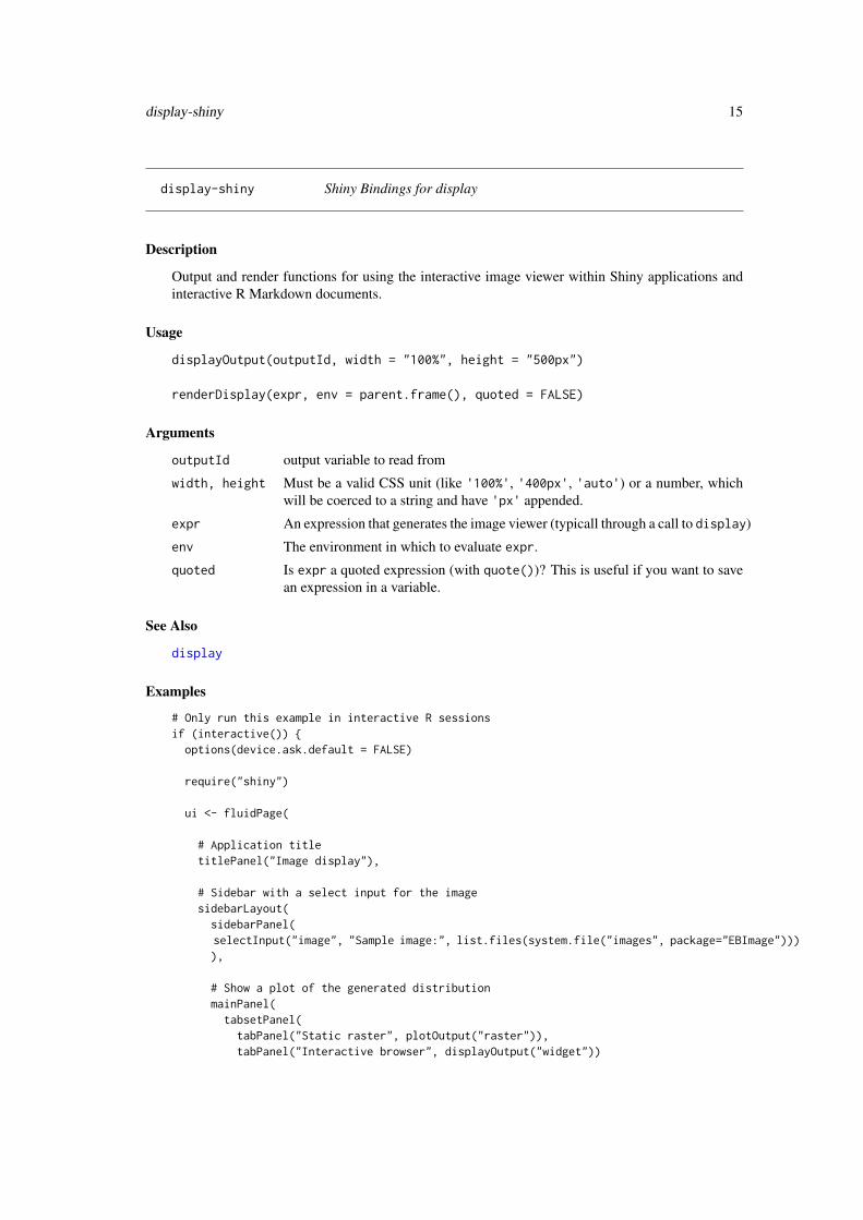
Output and render functions for using the interactive image viewer within Shiny applications andinteractive R Markdown documents.

Usage

displayOutput(outputId, width = "100%", height = "500px")

renderDisplay(expr, env = parent.frame(), quoted = FALSE)

Arguments

outputId output variable to read from

width, height Must be a valid CSS unit (like '100%', '400px', 'auto') or a number, whichwill be coerced to a string and have 'px' appended.

expr An expression that generates the image viewer (typicall through a call to display)

env The environment in which to evaluate expr.

quoted Is expr a quoted expression (with quote())? This is useful if you want to savean expression in a variable.

See Also

display

Examples

# Only run this example in interactive R sessionsif (interactive()) {

options(device.ask.default = FALSE)

require("shiny")

ui <- fluidPage(

# Application titletitlePanel("Image display"),

# Sidebar with a select input for the imagesidebarLayout(

sidebarPanel(selectInput("image", "Sample image:", list.files(system.file("images", package="EBImage")))),

# Show a plot of the generated distributionmainPanel(

tabsetPanel(tabPanel("Static raster", plotOutput("raster")),tabPanel("Interactive browser", displayOutput("widget"))

16 distmap

))

)

)

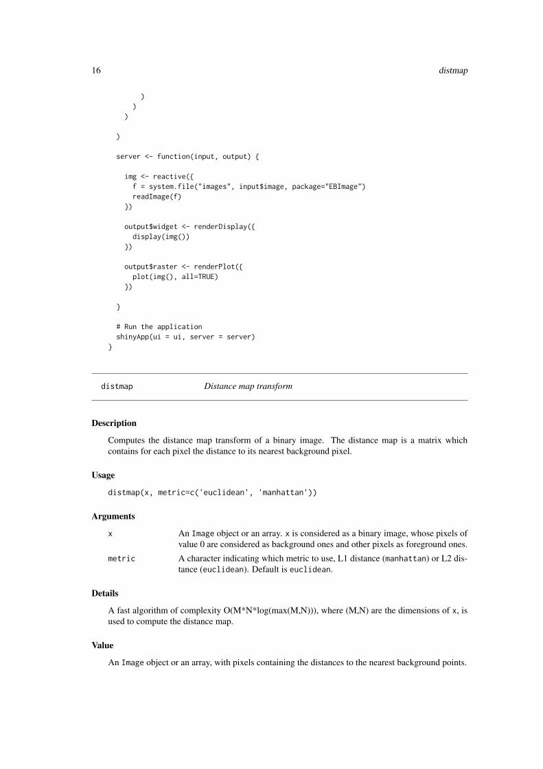
server <- function(input, output) {

img <- reactive({f = system.file("images", input$image, package="EBImage")readImage(f)

})

output$widget <- renderDisplay({display(img())

})

output$raster <- renderPlot({plot(img(), all=TRUE)

})

}

# Run the applicationshinyApp(ui = ui, server = server)

}

distmap Distance map transform

Description

Computes the distance map transform of a binary image. The distance map is a matrix whichcontains for each pixel the distance to its nearest background pixel.

Usage

distmap(x, metric=c('euclidean', 'manhattan'))

Arguments

x An Image object or an array. x is considered as a binary image, whose pixels ofvalue 0 are considered as background ones and other pixels as foreground ones.

metric A character indicating which metric to use, L1 distance (manhattan) or L2 dis-tance (euclidean). Default is euclidean.

Details

A fast algorithm of complexity O(M*N*log(max(M,N))), where (M,N) are the dimensions of x, isused to compute the distance map.

Value

An Image object or an array, with pixels containing the distances to the nearest background points.

drawCircle 17

Author(s)


References

M. N. Kolountzakis, K. N. Kutulakos. Fast Computation of the Euclidean Distance Map for BinaryImages, Infor. Proc. Letters 43 (1992).

Examples

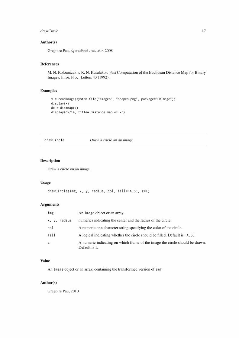
x = readImage(system.file("images", "shapes.png", package="EBImage"))display(x)dx = distmap(x)display(dx/10, title='Distance map of x')

drawCircle Draw a circle on an image.

Description

Draw a circle on an image.

Usage

drawCircle(img, x, y, radius, col, fill=FALSE, z=1)

Arguments

img An Image object or an array.

x, y, radius numerics indicating the center and the radius of the circle.

col A numeric or a character string specifying the color of the circle.

fill A logical indicating whether the circle should be filled. Default is FALSE.

z A numeric indicating on which frame of the image the circle should be drawn.Default is 1.

Value

An Image object or an array, containing the transformed version of img.

Author(s)

Gregoire Pau, 2010

18 EBImage

Examples

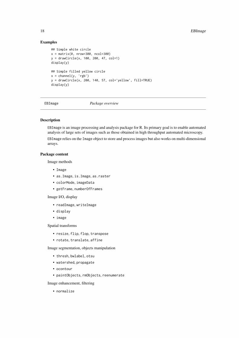
## Simple white circlex = matrix(0, nrow=300, ncol=300)y = drawCircle(x, 100, 200, 47, col=1)display(y)

## Simple filled yellow circlex = channel(y, 'rgb')y = drawCircle(x, 200, 140, 57, col='yellow', fill=TRUE)display(y)

EBImage Package overview

Description

EBImage is an image processing and analysis package for R. Its primary goal is to enable automatedanalysis of large sets of images such as those obtained in high throughput automated microscopy.

EBImage relies on the Image object to store and process images but also works on multi-dimensionalarrays.

Package content

Image methods

• Image

• as.Image, is.Image, as.raster

• colorMode, imageData

• getFrame, numberOfFrames

Image I/O, display

• readImage, writeImage

• display

• image

Spatial transforms

• resize, flip, flop, transpose

• rotate, translate, affine

Image segmentation, objects manipulation

• thresh, bwlabel, otsu

• watershed, propagate

• ocontour

• paintObjects, rmObjects, reenumerate

Image enhancement, filtering

• normalize

EBImage 19

• filter2, gblur, medianFilter

Morphological operations

• makeBrush

• erode, dilate, opening, closing• whiteTopHat, blackTopHat, selfComplementaryTopHat• distmap

• floodFill, fillHull

Color space manipulation

• rgbImage, channel, toRGB

Image stacking, combining, tiling

• stackObjects

• combine

• tile, untile

Drawing on images

• drawCircle

Features extraction

• computeFeatures

• computeFeatures.basic, computeFeatures.moment, computeFeatures.shape, computeFeatures.haralick• standardExpandRef

Defunct

• blur, equalize• drawtext, drawfont• getFeatures, hullFeatures, zernikeMoments• edgeProfile, edgeFeatures,• haralickFeatures, haralickMatrix• moments, cmoments, smoments, rmoments

Authors

Oleg Sklyar, <[email protected]>, Copyright 2005-2007

Gregoire Pau, <[email protected]>

Wolfgang Huber, <[email protected]>

Andrzej Oles, <[email protected]>

Mike Smith, <[email protected]>

European Bioinformatics InstituteEuropean Molecular Biology LaboratoryWellcome Trust Genome CampusHinxtonCambridge CB10 1SDUK

20 EBImage-defunct

The code of propagate is based on the CellProfiler with permission granted to distribute thisparticular part under LGPL, the corresponding copyright (Jones, Carpenter) applies.

The source code is released under LGPL (see the LICENSE file in the package root for the completelicense wording).

This library is free software; you can redistribute it and/or modify it under the terms of the GNULesser General Public License as published by the Free Software Foundation; either version 2.1of the License, or (at your option) any later version. This library is distributed in the hope that itwill be useful, but WITHOUT ANY WARRANTY; without even the implied warranty of MER-CHANTABILITY or FITNESS FOR A PARTICULAR PURPOSE.

See the GNU Lesser General Public License for more details. For LGPL license wording seehttp://www.gnu.org/licenses/lgpl.html

Examples

example(readImage)example(display)example(rotate)example(propagate)

EBImage-defunct Defunct functions in package ‘EBImage’

Description

These functions are defunct and no longer available.

Details

The following functions are defunct and no longer available; use the replacement indicated below.

• animate: display

• blur: gblur

• drawtext: see package vignette for documentation on how to add text labels to images

• drawfont: see package vignette for documentation on how to add text labels to images

• getFeatures: computeFeatures

• getNumberOfFrames: numberOfFrames

• hullFeatures: computeFeatures.shape

• zernikeMoments: computeFeatures

• edgeProfile: computeFeatures

• edgeFeatures: computeFeatures.shape

• haralickFeatures: computeFeatures

• haralickMatrix: computeFeatures

• moments: computeFeatures.moment

• cmoments: computeFeatures.moment

• rmoments: computeFeatures.moment

• smoments: computeFeatures.moment

http://www.gnu.org/licenses/lgpl.html

equalize 21

• dilateGreyScale: dilate

• erodeGreyScale: erode

• openingGreyScale: opening

• closingGreyScale: closing

• whiteTopHatGreyScale: whiteTopHat

• blackTopHatGreyScale: blackTopHat

• selfcomplementaryTopHatGreyScale: selfComplementaryTopHat

equalize Histogram Equalization

Description

Equalize the image histogram to a specified range and number of levels.

Usage

equalize(x, range = c(0, 1), levels = 256)

Arguments

x an Image object or an array

range numeric vector of length 2, the output range of the equalized histogram

levels number of grayscale levels (Grayscale images) or intensity levels of each chan-nel (Color images)

Details

Histogram equalization is an adaptive image contrast adjustment method. It flattens the imagehistogram by performing linearization of the cumulative distribution function of pixel intensities.

Individual channels of Color images and frames of image stacks are equalized separately.

Value

An Image object or an array, containing the transformed version of x.

Author(s)


See Also

clahe

22 fillHull

Examples

x = readImage(system.file('images', 'cells.tif', package='EBImage'))hist(x)y = equalize(x)hist(y)display(y, title='Equalized Grayscale Image')

x = readImage(system.file('images', 'sample-color.png', package='EBImage'))hist(x)y = equalize(x)hist(y)display(y, title='Equalized Grayscale Image')

fillHull Fill holes in objects

Description

Fill holes in objects.

Usage

fillHull(x)

Arguments


Details

fillHull fills holes in the objects defined in x, where objects are sets of pixels with the sameunique integer value.

Value


Author(s)

Gregoire Pau, Oleg Sklyar; 2007

See Also

bwlabel

filter2 23

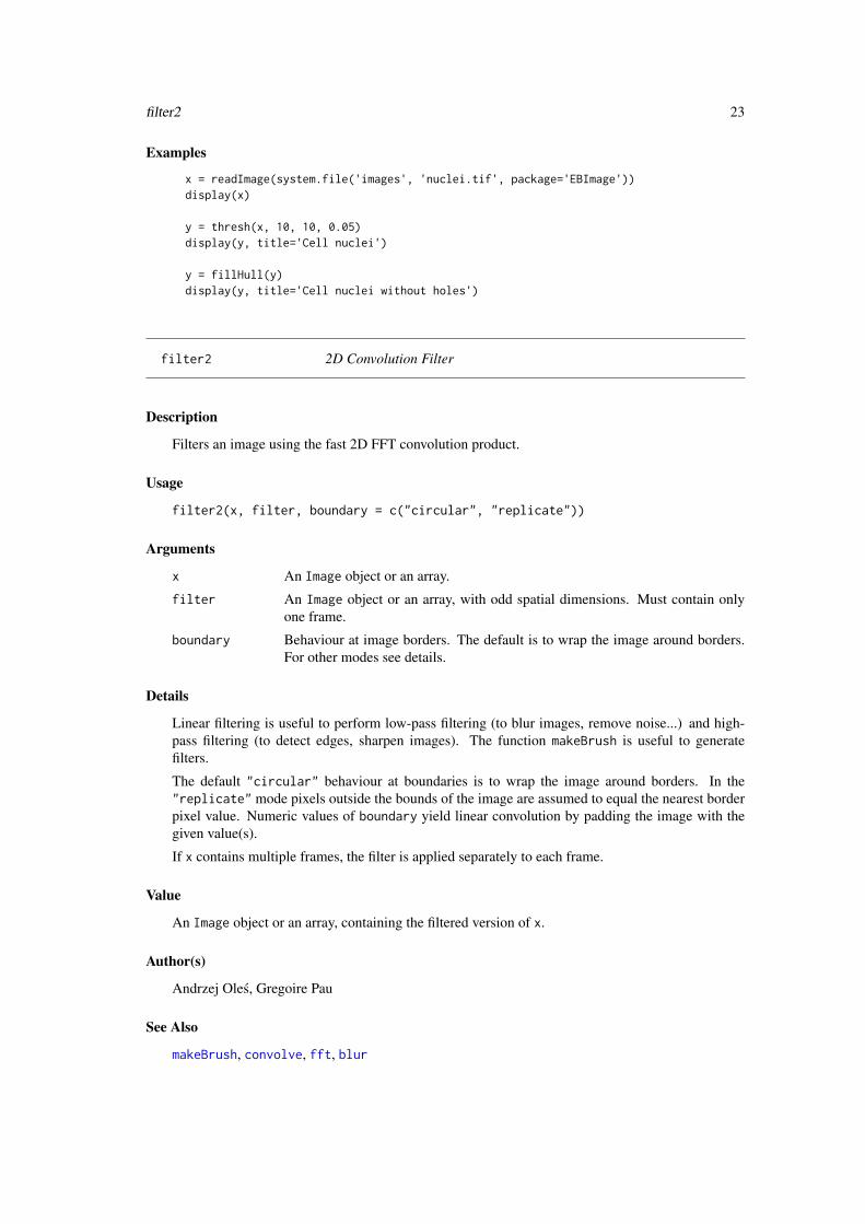
Examples

x = readImage(system.file('images', 'nuclei.tif', package='EBImage'))display(x)

y = thresh(x, 10, 10, 0.05)display(y, title='Cell nuclei')

y = fillHull(y)display(y, title='Cell nuclei without holes')

filter2 2D Convolution Filter

Description

Filters an image using the fast 2D FFT convolution product.

Usage

filter2(x, filter, boundary = c("circular", "replicate"))

Arguments


filter An Image object or an array, with odd spatial dimensions. Must contain onlyone frame.

boundary Behaviour at image borders. The default is to wrap the image around borders.For other modes see details.

Details

Linear filtering is useful to perform low-pass filtering (to blur images, remove noise...) and high-pass filtering (to detect edges, sharpen images). The function makeBrush is useful to generatefilters.

The default "circular" behaviour at boundaries is to wrap the image around borders. In the"replicate" mode pixels outside the bounds of the image are assumed to equal the nearest borderpixel value. Numeric values of boundary yield linear convolution by padding the image with thegiven value(s).

If x contains multiple frames, the filter is applied separately to each frame.

Value


Author(s)

Andrzej Oles, Gregoire Pau

See Also

makeBrush, convolve, fft, blur

24 floodFill

Examples

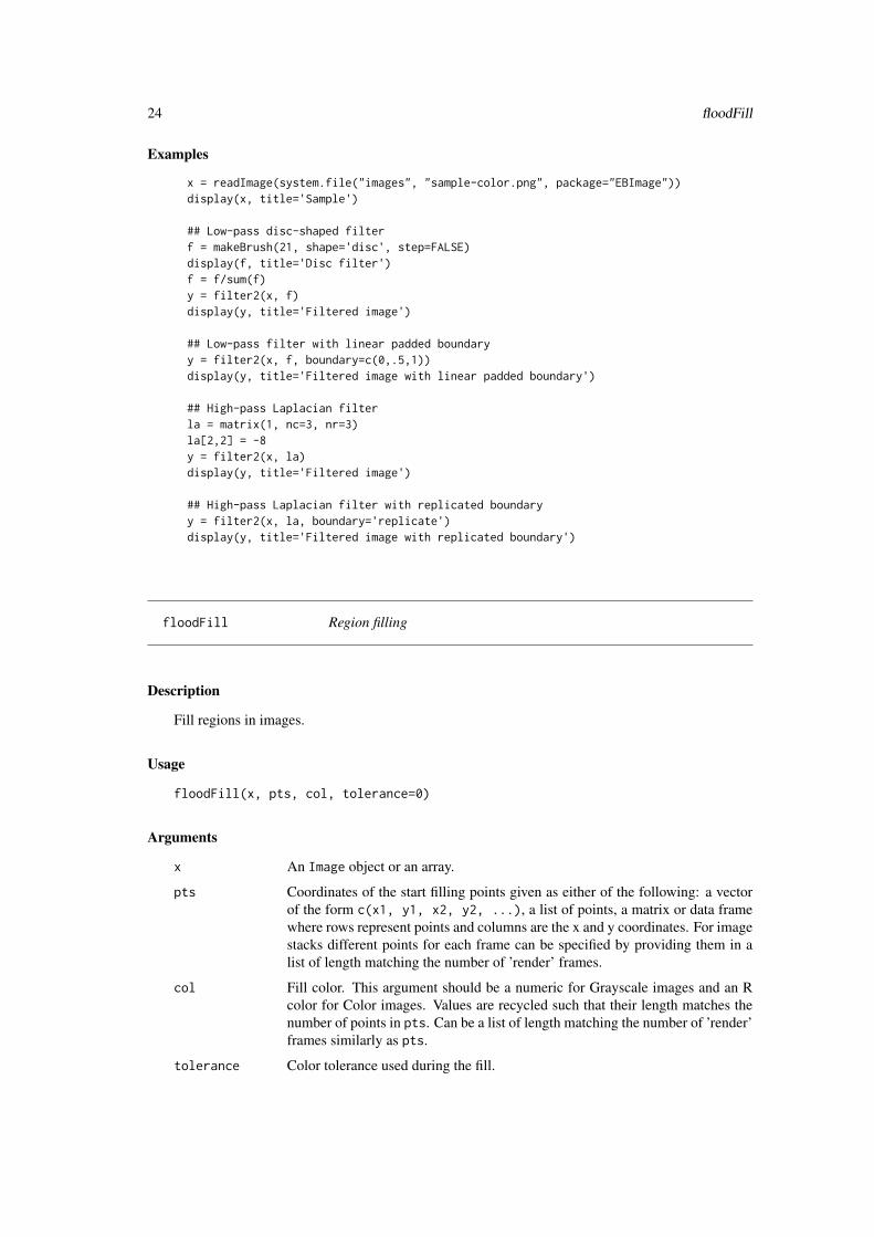
x = readImage(system.file("images", "sample-color.png", package="EBImage"))display(x, title='Sample')

## Low-pass disc-shaped filterf = makeBrush(21, shape='disc', step=FALSE)display(f, title='Disc filter')f = f/sum(f)y = filter2(x, f)display(y, title='Filtered image')

## Low-pass filter with linear padded boundaryy = filter2(x, f, boundary=c(0,.5,1))display(y, title='Filtered image with linear padded boundary')

## High-pass Laplacian filterla = matrix(1, nc=3, nr=3)la[2,2] = -8y = filter2(x, la)display(y, title='Filtered image')

## High-pass Laplacian filter with replicated boundaryy = filter2(x, la, boundary='replicate')display(y, title='Filtered image with replicated boundary')

floodFill Region filling

Description

Fill regions in images.

Usage

floodFill(x, pts, col, tolerance=0)

Arguments


pts Coordinates of the start filling points given as either of the following: a vectorof the form c(x1, y1, x2, y2, ...), a list of points, a matrix or data framewhere rows represent points and columns are the x and y coordinates. For imagestacks different points for each frame can be specified by providing them in alist of length matching the number of ’render’ frames.

col Fill color. This argument should be a numeric for Grayscale images and an Rcolor for Color images. Values are recycled such that their length matches thenumber of points in pts. Can be a list of length matching the number of ’render’frames similarly as pts.

tolerance Color tolerance used during the fill.

gblur 25

Details

Flood fill is performed using the fast scan line algorithm. Filling starts at pts and grows inconnected areas where the absolute difference of the pixels intensities (or colors) remains belowtolerance.

Value


Author(s)

Gregoire Pau, Oleg Sklyar; 2007

Examples

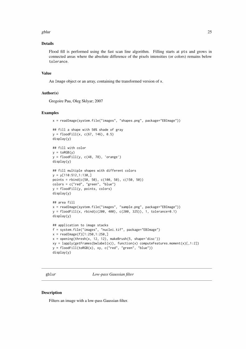
x = readImage(system.file("images", "shapes.png", package="EBImage"))

## fill a shape with 50% shade of grayy = floodFill(x, c(67, 146), 0.5)display(y)

## fill with colory = toRGB(y)y = floodFill(y, c(48, 78), 'orange')display(y)

## fill multiple shapes with different colorsy = y[110:512,1:130,]points = rbind(c(50, 50), c(100, 50), c(150, 50))colors = c("red", "green", "blue")y = floodFill(y, points, colors)display(y)

## area fillx = readImage(system.file("images", "sample.png", package="EBImage"))y = floodFill(x, rbind(c(200, 400), c(200, 325)), 1, tolerance=0.1)display(y)

## application to image stacksf = system.file("images", "nuclei.tif", package="EBImage")x = readImage(f)[1:250,1:250,]x = opening(thresh(x, 12, 12), makeBrush(5, shape='disc'))xy = lapply(getFrames(bwlabel(x)), function(x) computeFeatures.moment(x)[,1:2])y = floodFill(toRGB(x), xy, c("red", "green", "blue"))display(y)

gblur Low-pass Gaussian filter

Description

Filters an image with a low-pass Gaussian filter.

26 Image

Usage

gblur(x, sigma, radius = 2 * ceiling(3 * sigma) + 1, ...)

Arguments

x An Image object or an array.sigma A numeric denoting the standard deviation of the Gaussian filter used for blur-

ring.radius The radius of the filter in pixels. Default is 2*ceiling(3*sigma)+1).... Arguments passed to filter2.

Details

The Gaussian filter is created with the function makeBrush.

Value


Author(s)

Oleg Sklyar, <[email protected]>, 2005-2007

See Also

filter2, makeBrush

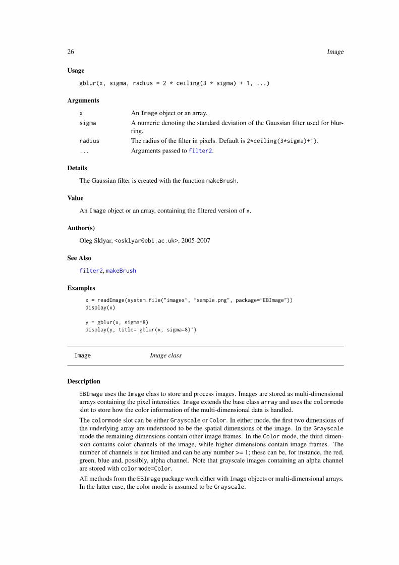
Examples

x = readImage(system.file("images", "sample.png", package="EBImage"))display(x)

y = gblur(x, sigma=8)display(y, title='gblur(x, sigma=8)')

Image Image class

Description

EBImage uses the Image class to store and process images. Images are stored as multi-dimensionalarrays containing the pixel intensities. Image extends the base class array and uses the colormodeslot to store how the color information of the multi-dimensional data is handled.

The colormode slot can be either Grayscale or Color. In either mode, the first two dimensions ofthe underlying array are understood to be the spatial dimensions of the image. In the Grayscalemode the remaining dimensions contain other image frames. In the Color mode, the third dimen-sion contains color channels of the image, while higher dimensions contain image frames. Thenumber of channels is not limited and can be any number >= 1; these can be, for instance, the red,green, blue and, possibly, alpha channel. Note that grayscale images containing an alpha channelare stored with colormode=Color.

All methods from the EBImage package work either with Image objects or multi-dimensional arrays.In the latter case, the color mode is assumed to be Grayscale.

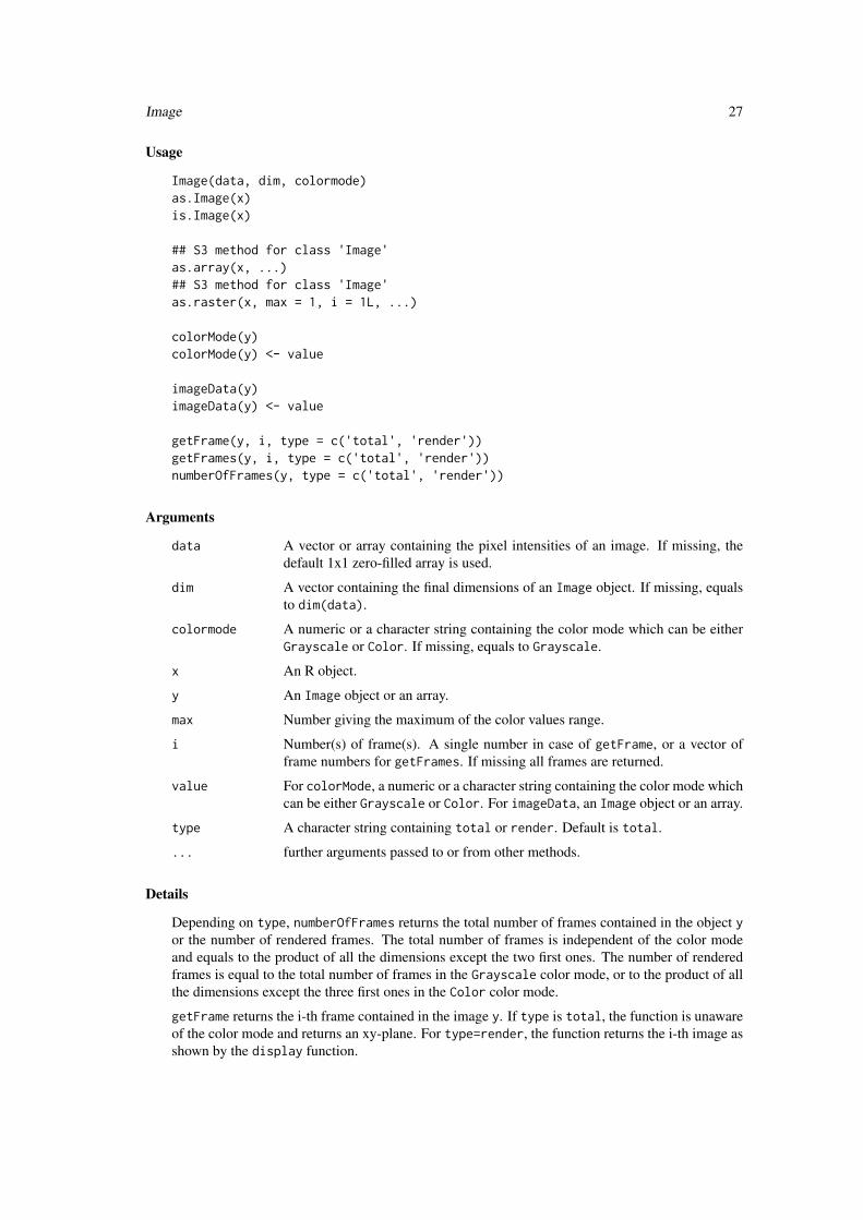
Image 27

Usage

Image(data, dim, colormode)as.Image(x)is.Image(x)

## S3 method for class 'Image'as.array(x, ...)## S3 method for class 'Image'as.raster(x, max = 1, i = 1L, ...)

colorMode(y)colorMode(y) <- value

imageData(y)imageData(y) <- value

getFrame(y, i, type = c('total', 'render'))getFrames(y, i, type = c('total', 'render'))numberOfFrames(y, type = c('total', 'render'))

Arguments

data A vector or array containing the pixel intensities of an image. If missing, thedefault 1x1 zero-filled array is used.

dim A vector containing the final dimensions of an Image object. If missing, equalsto dim(data).

colormode A numeric or a character string containing the color mode which can be eitherGrayscale or Color. If missing, equals to Grayscale.

x An R object.

y An Image object or an array.

max Number giving the maximum of the color values range.

i Number(s) of frame(s). A single number in case of getFrame, or a vector offrame numbers for getFrames. If missing all frames are returned.

value For colorMode, a numeric or a character string containing the color mode whichcan be either Grayscale or Color. For imageData, an Image object or an array.

type A character string containing total or render. Default is total.

... further arguments passed to or from other methods.

Details

Depending on type, numberOfFrames returns the total number of frames contained in the object yor the number of rendered frames. The total number of frames is independent of the color modeand equals to the product of all the dimensions except the two first ones. The number of renderedframes is equal to the total number of frames in the Grayscale color mode, or to the product of allthe dimensions except the three first ones in the Color color mode.

getFrame returns the i-th frame contained in the image y. If type is total, the function is unawareof the color mode and returns an xy-plane. For type=render, the function returns the i-th image asshown by the display function.

28 io

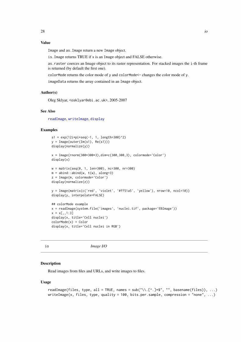
Value

Image and as.Image return a new Image object.

is.Image returns TRUE if x is an Image object and FALSE otherwise.

as.raster coerces an Image object to its raster representation. For stacked images the i-th frameis returned (by default the first one).

colorMode returns the color mode of y and colorMode<- changes the color mode of y.

imageData returns the array contained in an Image object.

Author(s)


See Also

readImage, writeImage, display

Examples

s1 = exp(12i*pi*seq(-1, 1, length=300)^2)y = Image(outer(Im(s1), Re(s1)))display(normalize(y))

x = Image(rnorm(300*300*3),dim=c(300,300,3), colormode='Color')display(x)

w = matrix(seq(0, 1, len=300), nc=300, nr=300)m = abind::abind(w, t(w), along=3)z = Image(m, colormode='Color')display(normalize(z))

y = Image(matrix(c('red', 'violet', '#ff51a5', 'yellow'), nrow=10, ncol=10))display(y, interpolate=FALSE)

## colorMode examplex = readImage(system.file('images', 'nuclei.tif', package='EBImage'))x = x[,,1:3]display(x, title='Cell nuclei')colorMode(x) = Colordisplay(x, title='Cell nuclei in RGB')

io Image I/O

Description

Read images from files and URLs, and write images to files.

Usage

readImage(files, type, all = TRUE, names = sub("\\.[^.]*$", "", basename(files)), ...)writeImage(x, files, type, quality = 100, bits.per.sample, compression = "none", ...)

io 29

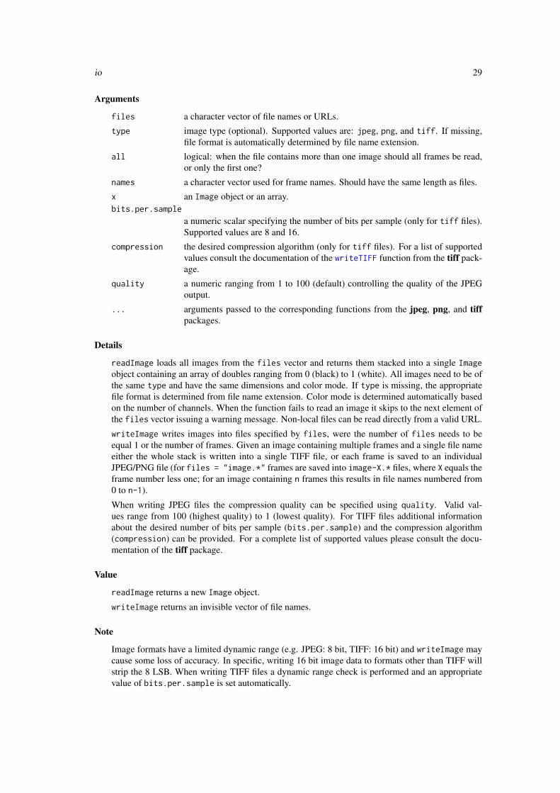
Arguments

files a character vector of file names or URLs.

type image type (optional). Supported values are: jpeg, png, and tiff. If missing,file format is automatically determined by file name extension.

all logical: when the file contains more than one image should all frames be read,or only the first one?

names a character vector used for frame names. Should have the same length as files.

x an Image object or an array.bits.per.sample

a numeric scalar specifying the number of bits per sample (only for tiff files).Supported values are 8 and 16.

compression the desired compression algorithm (only for tiff files). For a list of supportedvalues consult the documentation of the writeTIFF function from the tiff pack-age.

quality a numeric ranging from 1 to 100 (default) controlling the quality of the JPEGoutput.

... arguments passed to the corresponding functions from the jpeg, png, and tiffpackages.

Details

readImage loads all images from the files vector and returns them stacked into a single Imageobject containing an array of doubles ranging from 0 (black) to 1 (white). All images need to be ofthe same type and have the same dimensions and color mode. If type is missing, the appropriatefile format is determined from file name extension. Color mode is determined automatically basedon the number of channels. When the function fails to read an image it skips to the next element ofthe files vector issuing a warning message. Non-local files can be read directly from a valid URL.

writeImage writes images into files specified by files, were the number of files needs to beequal 1 or the number of frames. Given an image containing multiple frames and a single file nameeither the whole stack is written into a single TIFF file, or each frame is saved to an individualJPEG/PNG file (for files = "image.*" frames are saved into image-X.* files, where X equals theframe number less one; for an image containing n frames this results in file names numbered from0 to n-1).

When writing JPEG files the compression quality can be specified using quality. Valid val-ues range from 100 (highest quality) to 1 (lowest quality). For TIFF files additional informationabout the desired number of bits per sample (bits.per.sample) and the compression algorithm(compression) can be provided. For a complete list of supported values please consult the docu-mentation of the tiff package.

Value

readImage returns a new Image object.

writeImage returns an invisible vector of file names.

Note

Image formats have a limited dynamic range (e.g. JPEG: 8 bit, TIFF: 16 bit) and writeImage maycause some loss of accuracy. In specific, writing 16 bit image data to formats other than TIFF willstrip the 8 LSB. When writing TIFF files a dynamic range check is performed and an appropriatevalue of bits.per.sample is set automatically.

30 localCurvature

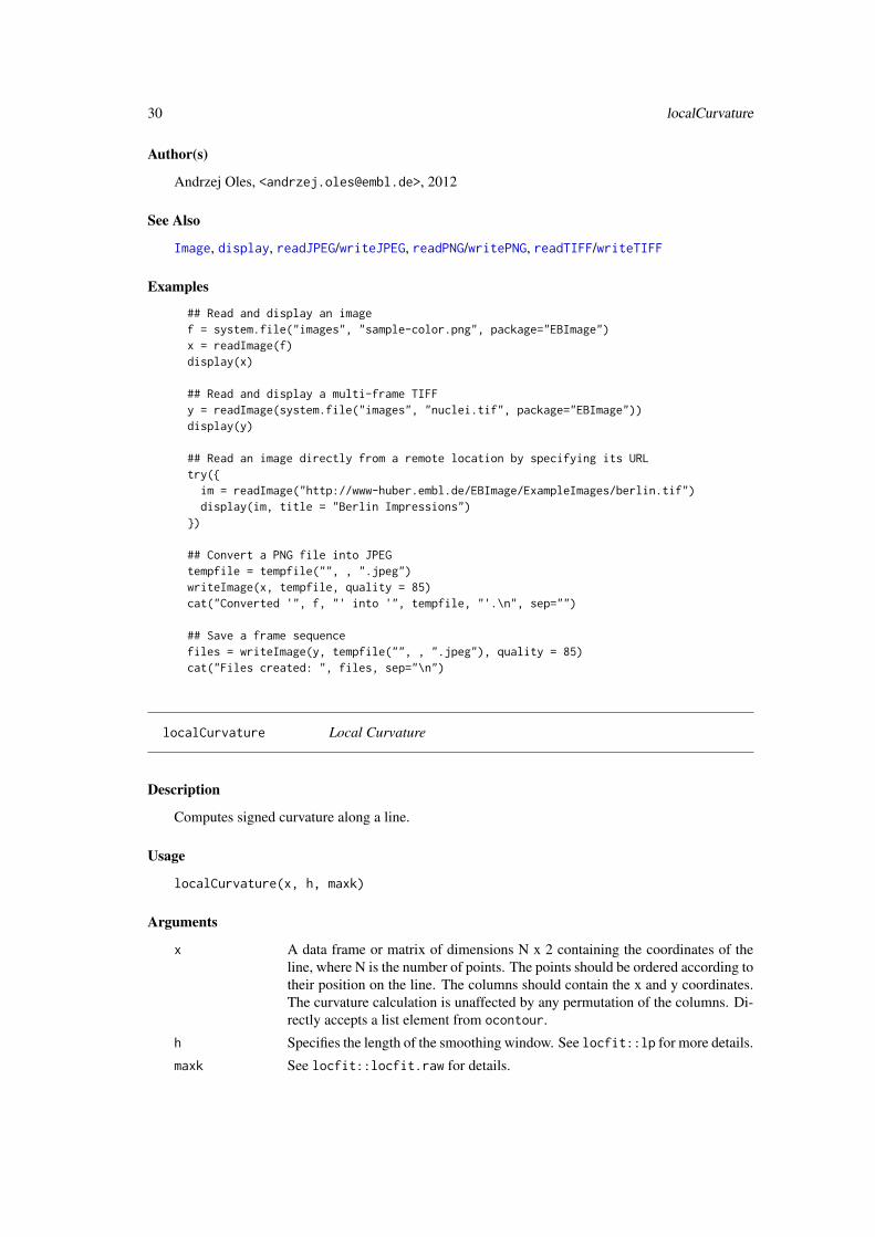
Author(s)


See Also

Image, display, readJPEG/writeJPEG, readPNG/writePNG, readTIFF/writeTIFF

Examples

## Read and display an imagef = system.file("images", "sample-color.png", package="EBImage")x = readImage(f)display(x)

## Read and display a multi-frame TIFFy = readImage(system.file("images", "nuclei.tif", package="EBImage"))display(y)

## Read an image directly from a remote location by specifying its URLtry({

im = readImage("http://www-huber.embl.de/EBImage/ExampleImages/berlin.tif")display(im, title = "Berlin Impressions")

})

## Convert a PNG file into JPEGtempfile = tempfile("", , ".jpeg")writeImage(x, tempfile, quality = 85)cat("Converted '", f, "' into '", tempfile, "'.\n", sep="")

## Save a frame sequencefiles = writeImage(y, tempfile("", , ".jpeg"), quality = 85)cat("Files created: ", files, sep="\n")

localCurvature Local Curvature

Description

Computes signed curvature along a line.

Usage

localCurvature(x, h, maxk)

Arguments

x A data frame or matrix of dimensions N x 2 containing the coordinates of theline, where N is the number of points. The points should be ordered according totheir position on the line. The columns should contain the x and y coordinates.The curvature calculation is unaffected by any permutation of the columns. Di-rectly accepts a list element from ocontour.

h Specifies the length of the smoothing window. See locfit::lp for more details.

maxk See locfit::locfit.raw for details.

medianFilter 31

Details

localCurvature fits a local non-parametric smoothing line (polynomial of degree 2) at each pointalong the line segment, and computes the curvature locally using numerical derivatives.

Value

Returns a list containing the contour coordinates x, the signed curvature at each point curvatureand the arc length of the contour length.

Author(s)

Joseph Barry, Wolfgang Huber, 2013

See Also

ocontour

Examples

## curvature goes as the inverse of the radius of a circlerange=seq(3.5,33.5,by=2)plotRange=seq(0.5,33.5,length=100)circleRes=array(dim=length(range))names(circleRes)=rangefor (i in seq_along(1:length(range))) {y=as.Image(makeBrush('disc', size=2*range[i]))y=ocontour(y)[[1]]circleRes[i]=abs(mean(localCurvature(x=y,h=range[i])$curvature, na.rm=TRUE))}plot(range, circleRes, ylim=c(0,max(circleRes, na.rm=TRUE)), xlab='Circle Radius', ylab='Curvature', type='p', xlim=range(plotRange))points(plotRange, 1/plotRange, type='l')

## Calculate curvaturex = readImage(system.file("images", "shapes.png", package="EBImage"))[25:74, 60:109]x = resize(x, 200)y = gblur(x, 3) > .3display(y)

contours = ocontour(bwlabel(y))c = localCurvature(x=contours[[1]], h=11)i = c$curvature >= 0pos = neg = array(0, dim(x))pos[c$contour[i,]+1] = c$curvature[i]neg[c$contour[!i,]+1] = -c$curvature[!i]display(10*(rgbImage(pos, , neg)), title = "Image curvature")

medianFilter 2D constant time median filtering

Description

Process an image using Perreault’s modern constant-time median filtering algorithm [1, 2].

32 medianFilter

Usage

medianFilter(x, size, cacheSize=512)

Arguments


size integer, median filter radius.

cacheSize integer, the L2 cache size of the system CPU in kB.

Details

Median filtering is useful as a smoothing technique, e.g. in the removal of speckling noise.

For a filter of radius size, the median kernel is a 2*size+1 times 2*size+1 square.

The input image x should contain pixel values in the range from 0 to 1, inclusive; values lower than0 or higher than 1 are clipped before applying the filter. Internal processing is performed using16-bit precision. The behavior at image boundaries is such as the source image has been paddedwith pixels whose values equal the nearest border pixel value.

If the image contains multiple channels or frames, the filter is applied to each one of them separately.

Value


Author(s)

Joseph Barry, <[email protected]>, 2012


References

[1] S. Perreault and P. Hebert, "Median Filtering in Constant Time", IEEE Trans Image Process16(9), 2389-2394, 2007

[2] http://nomis80.org/ctmf.html

See Also

gblur

Examples

x = readImage(system.file("images", "nuclei.tif", package="EBImage"))display(x, title='Nuclei')y = medianFilter(x, 5)display(y, title='Filtered nuclei')

http://nomis80.org/ctmf.html

morphology 33

morphology Perform morphological operations on images

Description

Functions to perform morphological operations on binary and grayscale images.

Usage

dilate(x, kern)erode(x, kern)opening(x, kern)closing(x, kern)whiteTopHat(x, kern)blackTopHat(x, kern)selfComplementaryTopHat(x, kern)

makeBrush(size, shape=c('box', 'disc', 'diamond', 'Gaussian', 'line'), step=TRUE, sigma=0.3, angle=45)

Arguments


kern An Image object or an array, containing the structuring element. kern is consid-ered as a binary image, with pixels of value 0 being the background and pixelswith values other than 0 being the foreground.

size A numeric containing the size of the brush in pixels. This should be an oddnumber; even numbers are rounded to the next odd one, i.e., size = 4 has thesame effect as size = 5. Default is 5

shape A character vector indicating the shape of the brush. Can be box, disc, diamond,Gaussian or line. Default is box.

step a logical indicating if the brush is binary. Default is TRUE. This argument isrelevant only for the disc and diamond shapes.

sigma An optional numeric containing the standard deviation of the Gaussian shape.Default is 0.3.

angle An optional numeric containing the angle at which the line should be drawn.The angle is one between the top of the image and the line.

Details

dilate applies the mask kern by positioning its center over every pixel of the image x, the outputvalue of the pixel is the maximum value of x covered by the mask. In case of binary images this isequivalent of putting the mask over every background pixel, and setting it to foreground if any ofthe pixels covered by the mask is from the foreground.

erode applies the mask kern by positioning its center over every pixel of the image x, the outputvalue of the pixel is the minimum value of x covered by the mask. In case of binary images this isequivalent of putting the mask over every foreground pixel, and setting it to background if any ofthe pixels covered by the mask is from the background.

opening is an erosion followed by a dilation and closing is a dilation followed by an erosion.

34 morphology

whiteTopHat returns the difference between the original image x and its opening by the structuringelement kern.

blackTopHat subtracts the original image x from its closing by the structuring element kern.

selfComplementaryTopHat is the sum of the whiteTopHat and the blackTopHat, simplified thedifference between the closing and the opening of the image.

makeBrush generates brushes of various sizes and shapes that can be used as structuring elements.

Processing Pixels at Image Borders (Padding Behavior): Morphological functions positionthe center of the structuring element over each pixel in the input image. For pixels close to theedge of an image, parts of the neighborhood defined by the structuring element may extend pastthe border of the image. In such a case, a value is assigned to these undefined pixels, as if theimage was padded with additional rows and columns. The value of these padding pixels variesfor dilation and erosion operations. For dilation, pixels beyond the image border are assigned theminimum value afforded by the data type, which in case of binary images is equivalent of settingthem to background. For erosion, pixels beyond the image border are assigned the maximumvalue afforded by the data type, which in case of binary images is equivalent of setting them toforeground.

Value

dilate, erode, opening, whiteTopHat, blackTopHat and selfComplementaryTopHat return thetransformed Image object or array x, after the corresponding morphological operation.

makeBrush generates a 2D matrix containing the desired brush.

Note

Morphological operations are implemented using the efficient Urbach-Wilkinson algorithm [1]. Itsrequired computing time is independent of both the image content and the number of gray levelsused.

Author(s)

Ilia Kats <<[email protected]>> (2012), Andrzej Oles <<[email protected]>> (2015)

References

[1] E. R. Urbach and M.H.F. Wilkinson, "Efficient 2-D grayscale morphological transformationswith arbitrary flat structuring elements", IEEE Trans Image Process 17(1), 1-8, 2008

Examples

x = readImage(system.file("images", "shapes.png", package="EBImage"))kern = makeBrush(5, shape='diamond')

display(x)display(kern, title='Structuring element')display(erode(x, kern), title='Erosion of x')display(dilate(x, kern), title='Dilatation of x')

## makeBrushdisplay(makeBrush(99, shape='diamond'))display(makeBrush(99, shape='disc', step=FALSE))display(2000*makeBrush(99, shape='Gaussian', sigma=10))

normalize 35

normalize Intensity values linear scaling

Description

Linearly scale the intensity values of an image to a specified range.

Usage

## S4 method for signature 'Image'normalize(object, separate=TRUE, ft=c(0,1), inputRange)

## S4 method for signature 'array'normalize(object, separate=TRUE, ft=c(0,1), inputRange)

Arguments

object an Image object or an array

separate if TRUE, normalizes each frame separately

ft a numeric vector of 2 values, target minimum and maximum intensity valuesafter normalization

inputRange a numeric vector of 2 values, sets the range of the input intensity values; valuesexceeding this range are clipped

Details

normalize performs linear interpolation of the intensity values of an image to the specified rangeft. If inputRange is not set the whole dynamic range of the image is used as input. By specifyinginputRange the input intensity range of the image can be limited to [min, max]. Values exceedingthis range are clipped, i.e. intensities lower/higher than min/max are set to min/max.

Value

An Image object or an array, containing the transformed version of object.

Author(s)

Oleg Sklyar, <[email protected]>, 2006-2007 Andrzej Oles, <[email protected]>, 2013

Examples

x = readImage(system.file('images', 'shapes.png', package='EBImage'))x = x[110:512,1:130]y = bwlabel(x)display(x, title='Original')

print(range(y))y = normalize(y)print(range(y))display(y, title='Segmented')

36 otsu

ocontour Oriented contours

Description

Computes the oriented contour of objects.

Usage

ocontour(x)

Arguments

x An Image object or an array, containing objects. Only integer values are consid-ered. Pixels of value 0 constitute the background. Each object is a set of pixelswith the same unique integer value. Objects are assumed connected.

Value

A list of matrices, containing the coordinates of object oriented contours.

Author(s)


Examples

x = readImage(system.file("images", "shapes.png", package="EBImage"))x = x[1:120,50:120]display(x)oc = ocontour(x)plot(oc[[1]], type='l')points(oc[[1]], col=2)

otsu Calculate Otsu’s threshold

Description

Returns a threshold value based on Otsu’s method, which can be then used to reduce the grayscaleimage to a binary image.

Usage

otsu(x, range = c(0, 1), levels = 256)

Arguments

x A Grayscale Image object or an array.

range Numeric vector of length 2 specifying the histogram range used for thresholding.

levels Number of grayscale levels.

paintObjects 37

Details

Otsu’s thresholding method [1] is useful to automatically perform clustering-based image thresh-olding. The algorithm assumes that the distribution of image pixel intensities follows a bi-modalhistogram, and separates those pixels into two classes (e.g. foreground and background). Theoptimal threshold value is determined by minimizing the combined intra-class variance.

The threshold value is calculated for each image frame separately resulting in a output vector oflength equal to the total number of frames in the image.

The default number of levels corresponds to the number of gray levels of an 8bit image. It isrecommended to adjust this value according to the bit depth of the processed data, i.e. set levelsto 2^16 = 65536 when working with 16bit images.

Value

A vector of length equal to the total number of frames in x. Each vector element contains the Otsu’sthreshold value calculated for the corresponding image frame.

Author(s)

Philip A. Marais <[email protected]>, Andrzej Oles <[email protected]>, 2014

References

[1] Nobuyuki Otsu, "A threshold selection method from gray-level histograms". IEEE Trans. Sys.,Man., Cyber. 9 (1): 62-66. doi:10.1109/TSMC.1979.4310076 (1979)

See Also

thresh

Examples

x = readImage(system.file("images", "sample.png", package="EBImage"))display(x)

## threshold using Otsu's methody = x > otsu(x)display(y)

paintObjects Mark objects in images

Description

Higlight objects in images by outlining and/or painting them.

Usage

paintObjects(x, tgt, opac=c(1, 1), col=c('red', NA), thick=FALSE, closed=FALSE)

38 paintObjects

Arguments

x An Image object in Grayscale color mode or an array containing object masks.Object masks are sets of pixels with the same unique integer value.

tgt An Image object or an array, containing the intensity values of the objects.

opac A numeric vector of two opacity values for drawing object boundaries and objectbodies. Opacity ranges from 0 to 1, with 0 being fully transparent and 1 fullyopaque.

col A character vector of two R colors for drawing object boundaries and objectbodies. By default, object boundaries are painted in red while object bodies arenot painted.

thick A logical indicating whether to use thick boundary contours. Default is FALSE.

closed A logical indicating whether object contours should be closed along image edgesor remain open.

Value

An Image object or an array, containing the painted version of tgt.

Author(s)

Oleg Sklyar, <[email protected]>, 2006-2007 Andrzej Oles, <[email protected]>, 2015

See Also

bwlabel, watershed, computeFeatures, colorLabels

Examples

## load imagesnuc = readImage(system.file('images', 'nuclei.tif', package='EBImage'))cel = readImage(system.file('images', 'cells.tif', package='EBImage'))img = rgbImage(green=cel, blue=nuc)display(img, title='Cells')

## segment nucleinmask = thresh(nuc, 10, 10, 0.05)nmask = opening(nmask, makeBrush(5, shape='disc'))nmask = fillHull(nmask)nmask = bwlabel(nmask)display(normalize(nmask), title='Cell nuclei mask')

## segment cells, using propagate and nuclei as 'seeds'ctmask = opening(cel>0.1, makeBrush(5, shape='disc'))cmask = propagate(cel, nmask, ctmask)display(normalize(cmask), title='Cell mask')

## using paintObjects to highlight objectsres = paintObjects(cmask, img, col='#ff00ff')res = paintObjects(nmask, res, col='#ffff00')display(res, title='Segmented cells')

propagate 39

propagate Voronoi-based segmentation on image manifolds

Description

Find boundaries between adjacent regions in an image, where seeds have been already identifiedin the individual regions to be segmented. The method finds the Voronoi region of each seed ona manifold with a metric controlled by local image properties. The method is motivated by theproblem of finding the borders of cells in microscopy images, given a labelling of the nuclei in theimages.

Algorithm and implementation are from Jones et al. [1].

Usage

propagate(x, seeds, mask=NULL, lambda=1e-4)

Arguments

x An Image object or an array, containing the image to segment.

seeds An Image object or an array, containing the seeding objects of the already iden-tified regions.

mask An optional Image object or an array, containing the binary image mask of theregions that can be segmented. If missing, the whole image is segmented.

lambda A numeric value. The regularization parameter used in the metric, determiningthe trade-off between the Euclidean distance in the image plane and the contri-bution of the gradient of x. See details.

Details

The method operates by computing a discretized approximation of the Voronoi regions for givenseed points on a Riemann manifold with a metric controlled by local image features.

Under this metric, the infinitesimal distance d between points v and v+dv is defined by:

d^2 = ( (t(dv)*g)^2 + lambda*t(dv)*dv )/(lambda + 1)

, where g is the gradient of image x at point v.

lambda controls the weight of the Euclidean distance term. When lambda tends to infinity, d tendsto the Euclidean distance. When lambda tends to 0, d tends to the intensity gradient of the image.

The gradient is computed on a neighborhood of 3x3 pixels.

Segmentation of the Voronoi regions in the vicinity of flat areas (having a null gradient) with smallvalues of lambda can suffer from artifacts coming from the metric approximation.

Value

An Image object or an array, containing the labelled objects.

License

The implementation is based on CellProfiler C++ source code [2, 3]. An LGPL license was grantedby Thouis Jones to use this part of CellProfiler’s code for the propagate function.

40 propagate

Author(s)

The original CellProfiler code is from Anne Carpenter <[email protected]>, Thouis Jones<[email protected]>, In Han Kang <[email protected]>. Responsible for this implementation:Greg Pau.

References

[1] T. Jones, A. Carpenter and P. Golland, "Voronoi-Based Segmentation of Cells on Image Mani-folds", CVBIA05 (535-543), 2005

[2] A. Carpenter, T.R. Jones, M.R. Lamprecht, C. Clarke, I.H. Kang, O. Friman, D. Guertin, J.H.Chang, R.A. Lindquist, J. Moffat, P. Golland and D.M. Sabatini, "CellProfiler: image analysissoftware for identifying and quantifying cell phenotypes", Genome Biology 2006, 7:R100

[3] CellProfiler: http://www.cellprofiler.org

See Also

bwlabel, watershed

Examples

## a paraboloid mountain in a planen = 400x = (n/4)^2 - matrix(

(rep(1:n, times=n) - n/2)^2 + (rep(1:n, each=n) - n/2)^2,nrow=n, ncol=n)

x = normalize(x)

## 4 seedsseeds = array(0, dim=c(n,n))seeds[51:55, 301:305] = 1seeds[301:305, 101:105] = 2seeds[201:205, 141:145] = 3seeds[331:335, 351:355] = 4

lambda = 10^seq(-8, -1, by=1)segmented = Image(dim=c(dim(x), length(lambda)))

for(i in seq_along(lambda)) {prop = propagate(x, seeds, lambda=lambda[i])prop = prop/max(prop)segmented[,,i] = prop

}

display(x, title='Image')display(seeds/max(seeds), title='Seeds')display(segmented, title="Voronoi regions", all=TRUE)

resize 41

resize Spatial linear transformations

Description

The following functions perform all spatial linear transforms: reflection, rotation, translation, resiz-ing, and general affine transform.

Usage

flip(x)flop(x)rotate(x, angle, filter = "bilinear", output.dim, output.origin, ...)translate(x, v, filter = "none", ...)resize(x, w, h, output.dim = c(w, h), output.origin = c(0, 0), antialias = FALSE, ...)

affine(x, m, filter = c("bilinear", "none"), output.dim, bg.col = "black", antialias = TRUE)

Arguments


angle A numeric specifying the image rotation angle in degrees.

v A vector of 2 numbers denoting the translation vector in pixels.

w, h Width and height of the resized image. One of these arguments can be missingto enable proportional resizing.

filter A character string indicating the interpolating sampling filter. Valid values are’none’ or ’bilinear’. See Details.

output.dim A vector of 2 numbers indicating the dimension of the output image. For affineand translate the default is dim(x), for resize it equals c(w, h), and forrotate it defaults to the bounding box size of the rotated image.

output.origin A vector of 2 numbers indicating the output coordinates of the origin in pixels.

m A 3x2 matrix describing the affine transformation. See Details.

bg.col Color used to fill the background pixels, defaults to "black". In the case of multi-frame images the value is recycled, and individual background for each framecan be specified by providing a vector.

antialias If TRUE, perform bilinear sampling at image edges using bg.col.

... Arguments to be passed to affine, such as filter, output.dim, bg.col orantialias.

Details

flip mirrors x around the image horizontal axis (vertical reflection).

flop mirrors x around the image vertical axis (horizontal reflection).

rotate rotates the image clockwise by the given angle around the origin specified in output.origin.If no output.origin is provided, the result will be centered in a recalculated bounding box unlessoutput.dim is provided.

42 rmObjects

resize scales the image x to the desired dimensions. The transformation origin can be specifiedin output.origin. For example, zooming about the output.origin can be achieved by settingoutput.dim to a value different from c(w, h).

affine returns the affine transformation of x, where pixels coordinates, denoted by the matrix px,are transformed to cbind(px, 1)%*%m.

All spatial transformations except flip and flop are based on the general affine transformation.Spatial interpolation can be either none, also called nearest neighbor, where the resulting pixel valueequals to the closest pixel value, or bilinear, where the new pixel value is computed by bilinearapproximation of the 4 neighboring pixels. The bilinear filter gives smoother results.

Value


Author(s)

Gregoire Pau, 2012

See Also

transpose

Examples

x <- readImage(system.file("images", "sample.png", package="EBImage"))display(x)

display( flip(x) )display( flop(x) )display( resize(x, 128) )display( rotate(x, 30) )display( translate(x, c(120, -20)) )

m <- matrix(c(0.6, 0.2, 0, -0.2, 0.3, 300), nrow=3)display( affine(x, m) )

rmObjects Object removal and re-indexation

Description

The rmObjects functions deletes objects from an image by setting their pixel intensity values to 0.reenumerate re-enumerates all objects in an image from 0 (background) to the actual number ofobjects.

Usage

rmObjects(x, index, reenumerate = TRUE)

reenumerate(x)

rmObjects 43

Arguments

x An Image object in Grayscale color mode or an array containing object masks.Object masks are sets of pixels with the same unique integer value.

index A numeric vector (or a list of vectors if x contains multiple frames) containingthe indexes of objects to remove in the frame.

reenumerate Logical, should all the objects in the image be re-indexed afterwards (default).

Value

An Image object or an array, containing the new objects.

Author(s)


See Also

bwlabel, watershed

Examples

## make objectsx = readImage(system.file('images', 'shapes.png', package='EBImage'))x = x[110:512,1:130]y = bwlabel(x)

## number of objects foundmax(y)

display(normalize(y), title='Objects')

## remove every second letterobjects = list(

seq.int(from = 2, to = max(y), by = 2),seq.int(from = 1, to = max(y), by = 2))

z = rmObjects(combine(y, y), objects)

display(normalize(z), title='Object removal')

## the number of objects left in each imageapply(z, 3, max)

## perform object removal without re-enumeratingz = rmObjects(y, objects, reenumerate = FALSE)

## labels of objects leftunique(as.vector(z))[-1L]

## re-index objectsz = reenumerate(z)unique(as.vector(z))[-1L]

44 stackObjects

stackObjects Places detected objects into an image stack

Description

Places detected objects into an image stack.

Usage

stackObjects(x, ref, combine=TRUE, bg.col='black', ext)

Arguments

x An Image object or an array containing object masks. Object masks are sets ofpixels with the same unique integer value.

ref An Image object or an array, containing the intensity values of the objects.

combine If x contains multiple images, specifies if the resulting list of image stacks withindividual objects should be combined using combine into a single image stack.

bg.col Background pixel color.

ext A numeric controlling the size of the output image. If missing, ext is estimatedfrom data. See details.

Details

stackObjects creates a set of n images of size (2*ext+1, 2*ext+1), where n is the number ofobjects in x, and places each object of x in this set.

If not specified, ext is estimated using the 98% quantile of m.majoraxis/2, where m.majoraxis isthe semi-major axis descriptor extracted from computeFeatures.moment, taken over all the objectsof the image x.

Value

An Image object containing the stacked objects contained in x. If x contains multiple images and ifcombine is TRUE, stackObjects returns a list of Image objects.

Author(s)


See Also

combine, tile, computeFeatures.moment

Examples

## simple examplex = readImage(system.file('images', 'shapes.png', package='EBImage'))x = x[110:512,1:130]y = bwlabel(x)display(normalize(y), title='Objects')z = stackObjects(y, normalize(y))

thresh 45

display(z, title='Stacked objects')

## load imagesnuc = readImage(system.file('images', 'nuclei.tif', package='EBImage'))cel = readImage(system.file('images', 'cells.tif', package='EBImage'))img = rgbImage(green=cel, blue=nuc)display(img, title='Cells')

## segment nucleinmask = thresh(nuc, 10, 10, 0.05)nmask = opening(nmask, makeBrush(5, shape='disc'))nmask = fillHull(bwlabel(nmask))

## segment cells, using propagate and nuclei as 'seeds'ctmask = opening(cel>0.1, makeBrush(5, shape='disc'))cmask = propagate(cel, nmask, ctmask)

## using paintObjects to highlight objectsres = paintObjects(cmask, img, col='#ff00ff')res = paintObjects(nmask, res, col='#ffff00')display(res, title='Segmented cells')

## stacked cellsst = stackObjects(cmask, img)display(st, title='Stacked objects')

thresh Adaptive thresholding

Description

Thresholds an image using a moving rectangular window.

Usage

thresh(x, w=5, h=5, offset=0.01)

Arguments


w, h Half width and height of the moving rectangular window.

offset Thresholding offset from the averaged value.

Details

This function returns the binary image resulting from the comparison between an image and its fil-tered version with a rectangular window. It is equivalent of doing { f = matrix(1, nc=2*w+1, nr=2*h+1);f = f/sum(f); x > (filter2(x, f, boundary="replicate") + offset) } but faster.The function filter2 provides hence more flexibility than thresh.

Value


46 tile

Author(s)


See Also

filter2

Examples

x = readImage(system.file('images', 'nuclei.tif', package='EBImage'))display(x)y = thresh(x, 10, 10, 0.05)display(y)

tile Tiling/untiling images

Description

Given a sequence of frames, tile generates a single image with frames tiled. untile is the inversefunction and divides an image into a sequence of images.

Usage

tile(x, nx=10, lwd=1, fg.col="#E4AF2B", bg.col="gray")untile(x, nim, lwd=1)

Arguments

x An Image object, an array or a list of these objects.

nx The number of tiled images in a row.

lwd The width of the grid lines between tiled images, can be 0.

fg.col The color of the grid lines.

bg.col The color of the background for extra tiles.

nim A numeric vector of 2 elements for the number of images in both directions.

Details

After object segmentation, tile is a useful addition to stackObjects to have an overview of thesegmented objects.

Value

An Image object or an array, containing the tiled/untiled version of x.

Author(s)


transpose 47

See Also

stackObjects

Examples

## make a set of blurred imagesimg = readImage(system.file("images", "sample-color.png", package="EBImage"))[257:768,,]x = resize(img, 128, 128)xt = list()for (t in seq(0.1, 5, len=9)) xt=c(xt, list(gblur(x, s=t)))xt = combine(xt)display(xt, title='Blurred images')

## tilext = tile(xt, 3)display(xt, title='Tiles')

## untilexu = untile(img, c(3, 3))display(xu, title='Blocks')

transpose Image Transposition

Description

Transposes an image by swapping its spatial dimensions.

Usage

transpose(x)

Arguments


Details

The transposition of an image is performed by swapping the X and Y indices of its array represen-tation.

Value

A transformed version of x with its first two dimensions transposed.

Note

The function is implemented using an efficient cash-oblivious algorithm which is typically fasterthan R’s aperm and t functions.

Author(s)

Andrzej Oles, <[email protected]>, 2012-2017

48 watershed

See Also

flip, flop, rotate

Examples

x = readImage(system.file("images", "sample-color.png", package="EBImage"))y = transpose(x)

display(x, title='Original')display(y, title='Transposed')

## performing the transposition of an image twice should result in the original imagez = transpose(y)identical(x, z)

watershed Watershed transformation and watershed based object detection

Description

Watershed transformation and watershed based object detection.

Usage

watershed(x, tolerance=1, ext=1)

Arguments


tolerance The minimum height of the object in the units of image intensity between itshighest point (seed) and the point where it contacts another object (checked forevery contact pixel). If the height is smaller than the tolerance, the object willbe combined with one of its neighbors, which is the highest. Tolerance shouldbe chosen according to the range of x. Default value is 1, which is a reasonablevalue if x comes from distmap.

ext Radius of the neighborhood in pixels for the detection of neighboring objects.Higher value smoothes out small objects.

Details

The algorithm identifies and separates objects that stand out of the background (zero). It inverts theimage and uses water to fill the resulting valleys (pixels with high intensity in the source image)until another object or background is met. The deepest valleys become indexed first, starting from1.

The function bwlabel is a simpler, faster alternative to segment connected objects from binaryimages.

Value

An Grayscale Image object or an array, containing the labelled version of x.

watershed 49

Author(s)

Oleg Sklyar, <[email protected]>, 2007

See Also

bwlabel, propagate

Examples

x = readImage(system.file('images', 'shapes.png', package='EBImage'))x = x[110:512,1:130]display(x, title='Binary')y = distmap(x)display(normalize(y), title='Distance map')w = watershed(y)display(normalize(w), title='Watershed')

Index

∗Topic manipotsu, 36thresh, 45tile, 46watershed, 48

∗Topic methodsabind, 2

∗Topic packageEBImage, 18EBImage-defunct, 20

[,Image,ANY,ANY,ANY-method (Image), 26[,Image-method (Image), 26

abind, 2, 2, 3, 9abind,ANY-method (abind), 2abind,Image-method (abind), 2abind,list-method (abind), 2abind-methods (abind), 2affine (resize), 41animate (EBImage-defunct), 20as.array.Image (Image), 26as.Image (Image), 26as.raster.Image (Image), 26

blackTopHat, 21blackTopHat (morphology), 33blackTopHatGreyScale (EBImage-defunct),

20blur, 23blur (EBImage-defunct), 20bwlabel, 3, 8, 12, 22, 38, 40, 43, 49

channel, 4clahe, 6, 21closing, 21closing (morphology), 33closingGreyScale (EBImage-defunct), 20cmoments (EBImage-defunct), 20Color (Image), 26colorLabels, 4, 7, 38colormap, 8colorMode, 5colorMode (Image), 26colormode (Image), 26

colorMode<- (Image), 26combine, 3, 9, 44combine,ANY,NULL-method (combine), 9combine,array,array-method (combine), 9combine,Image,Image-method (combine), 9combine,list,missing-method (combine), 9combine,matrix,matrix-method (combine),

9combine,NULL,ANY-method (combine), 9combine,NULL,NULL-method (combine), 9computeFeatures, 4, 10, 20, 38computeFeatures.moment, 20, 44computeFeatures.shape, 20convolve, 23createWidget, 13

dilate, 21dilate (morphology), 33dilateGreyScale (EBImage-defunct), 20display, 12, 15, 20, 28, 30display-shiny, 15displayOutput (display-shiny), 15distmap, 16drawCircle, 17drawfont (EBImage-defunct), 20drawtext (EBImage-defunct), 20

EBImage, 18EBImage-defunct, 20edgeFeatures (EBImage-defunct), 20edgeProfile (EBImage-defunct), 20equalize, 7, 21erode, 21erode (morphology), 33erodeGreyScale (EBImage-defunct), 20

fft, 23fillHull, 22filter2, 11, 23, 26flip, 48flip (resize), 41floodFill, 24flop, 48flop (resize), 41

50

INDEX 51

gblob (computeFeatures), 10gblur, 20, 25, 32getFeatures (EBImage-defunct), 20getFrame (Image), 26getFrames (Image), 26getNumberOfFrames (EBImage-defunct), 20Grayscale (Image), 26

haralickFeatures (EBImage-defunct), 20haralickMatrix (EBImage-defunct), 20hist,Image-method (Image), 26hullFeatures (EBImage-defunct), 20

Image, 26, 30image,Image-method (Image), 26Image-class (Image), 26imageData (Image), 26imageData<- (Image), 26io, 28is.Image (Image), 26

localCurvature, 30log,Image-method (Image), 26

makeBrush, 23, 26makeBrush (morphology), 33Math2,Image-method (Image), 26median.Image (Image), 26medianFilter, 31moments (EBImage-defunct), 20morphology, 33

normalize, 8, 35normalize,array-method (normalize), 35normalize,Image-method (normalize), 35normalize,matrix-method (normalize), 35numberOfFrames, 20numberOfFrames (Image), 26

ocontour, 31, 36opening, 21opening (morphology), 33openingGreyScale (EBImage-defunct), 20Ops,Image,Image-method (Image), 26Ops,Image,numeric-method (Image), 26Ops,numeric,Image-method (Image), 26otsu, 36

paintObjects, 4, 37par, 14plot.Image (display), 12print.Image (Image), 26propagate, 4, 12, 20, 39, 49

quantile.Image (Image), 26

readImage, 28readImage (io), 28readJPEG, 30readPNG, 30readTIFF, 30reenumerate (rmObjects), 42renderDisplay (display-shiny), 15resize, 41rgbImage (channel), 4rmObjects, 42rmoments (EBImage-defunct), 20rotate, 48rotate (resize), 41

selfComplementaryTopHat, 21selfComplementaryTopHat (morphology), 33selfcomplementaryTopHatGreyScale

(EBImage-defunct), 20show,Image-method (Image), 26smoments (EBImage-defunct), 20stackObjects, 44, 47standardExpandRef (computeFeatures), 10

thresh, 37, 45tile, 3, 44, 46toRGB (channel), 4translate (resize), 41transpose, 42, 47

untile (tile), 46

watershed, 4, 38, 40, 43, 48whiteTopHat, 21whiteTopHat (morphology), 33whiteTopHatGreyScale (EBImage-defunct),

20writeImage, 28writeImage (io), 28writeJPEG, 30writePNG, 30writeTIFF, 29, 30

zernikeMoments (EBImage-defunct), 20

Package ‘EBImage’ - Bioconductor ‘EBImage ’ April 11, 2018 ... display(z, title=’Colored...

Documents

Transcript of Package ‘EBImage’ - Bioconductor ‘EBImage ’ April 11, 2018 ... display(z, title=’Colored...