Package ‘arﬁma’ - The Comprehensive R Archive Network have ﬁxed = list(phi = c(0, NA)). NA...

Package ‘arfima’June 19, 2018

Title Fractional ARIMA (and Other Long Memory) Time Series Modeling

Version 1.6-7

Date 2018-06-19

Author JQ (Justin) Veenstra [aut, cre], A.I. McLeod [aut]

Maintainer JQ Veenstra <[email protected]>

Depends R (>= 3.0.0), ltsa

Imports parallel

Description Simulates, fits, and predicts long-memory and anti-persistenttime series, possibly mixed with ARMA, regression, transfer-functioncomponents.Exact methods (MLE, forecasting, simulation) are used.Bug reports should be done via GitHub (at<https://github.com/JQVeenstra/arfima>), where the development versionof this package lives; it can be installed using devtools.

License MIT + file LICENSE

RoxygenNote 6.0.1

NeedsCompilation yes

Repository CRAN

Date/Publication 2018-06-19 20:19:20 UTC

R topics documented:arfima-package . . . . . . . . . . . . . . . . . . . . . . . . . . . . . . . . . . . . . . . 2AIC.arfima . . . . . . . . . . . . . . . . . . . . . . . . . . . . . . . . . . . . . . . . . 5arfima . . . . . . . . . . . . . . . . . . . . . . . . . . . . . . . . . . . . . . . . . . . . 6arfima.sim . . . . . . . . . . . . . . . . . . . . . . . . . . . . . . . . . . . . . . . . . . 10arfima0 . . . . . . . . . . . . . . . . . . . . . . . . . . . . . . . . . . . . . . . . . . . 12arfimachanges . . . . . . . . . . . . . . . . . . . . . . . . . . . . . . . . . . . . . . . . 13ARToPacf . . . . . . . . . . . . . . . . . . . . . . . . . . . . . . . . . . . . . . . . . . 13bestModes . . . . . . . . . . . . . . . . . . . . . . . . . . . . . . . . . . . . . . . . . . 14coef.arfima . . . . . . . . . . . . . . . . . . . . . . . . . . . . . . . . . . . . . . . . . 15distance . . . . . . . . . . . . . . . . . . . . . . . . . . . . . . . . . . . . . . . . . . . 16

1

2 arfima-package

fitted.arfima . . . . . . . . . . . . . . . . . . . . . . . . . . . . . . . . . . . . . . . . . 17iARFIMA . . . . . . . . . . . . . . . . . . . . . . . . . . . . . . . . . . . . . . . . . . 18IdentInvertQ . . . . . . . . . . . . . . . . . . . . . . . . . . . . . . . . . . . . . . . . . 19lARFIMA . . . . . . . . . . . . . . . . . . . . . . . . . . . . . . . . . . . . . . . . . . 21lARFIMAwTF . . . . . . . . . . . . . . . . . . . . . . . . . . . . . . . . . . . . . . . 23logLik.arfima . . . . . . . . . . . . . . . . . . . . . . . . . . . . . . . . . . . . . . . . 24PacfToAR . . . . . . . . . . . . . . . . . . . . . . . . . . . . . . . . . . . . . . . . . . 25plot.predarfima . . . . . . . . . . . . . . . . . . . . . . . . . . . . . . . . . . . . . . . 26plot.tacvf . . . . . . . . . . . . . . . . . . . . . . . . . . . . . . . . . . . . . . . . . . 27predict.arfima . . . . . . . . . . . . . . . . . . . . . . . . . . . . . . . . . . . . . . . . 28print.arfima . . . . . . . . . . . . . . . . . . . . . . . . . . . . . . . . . . . . . . . . . 30print.predarfima . . . . . . . . . . . . . . . . . . . . . . . . . . . . . . . . . . . . . . . 31print.summary.arfima . . . . . . . . . . . . . . . . . . . . . . . . . . . . . . . . . . . . 32print.tacvf . . . . . . . . . . . . . . . . . . . . . . . . . . . . . . . . . . . . . . . . . . 33removeMode . . . . . . . . . . . . . . . . . . . . . . . . . . . . . . . . . . . . . . . . 34residuals.arfima . . . . . . . . . . . . . . . . . . . . . . . . . . . . . . . . . . . . . . . 35SeriesJ . . . . . . . . . . . . . . . . . . . . . . . . . . . . . . . . . . . . . . . . . . . . 36summary.arfima . . . . . . . . . . . . . . . . . . . . . . . . . . . . . . . . . . . . . . . 37tacfplot . . . . . . . . . . . . . . . . . . . . . . . . . . . . . . . . . . . . . . . . . . . 38tacvf . . . . . . . . . . . . . . . . . . . . . . . . . . . . . . . . . . . . . . . . . . . . . 39tacvfARFIMA . . . . . . . . . . . . . . . . . . . . . . . . . . . . . . . . . . . . . . . . 40tmpyr . . . . . . . . . . . . . . . . . . . . . . . . . . . . . . . . . . . . . . . . . . . . 42vcov.arfima . . . . . . . . . . . . . . . . . . . . . . . . . . . . . . . . . . . . . . . . . 43weed . . . . . . . . . . . . . . . . . . . . . . . . . . . . . . . . . . . . . . . . . . . . . 45

Index 47

arfima-package Simulates, fits, and predicts persistent and anti-persistent time series.arfima

Description

Simulates with arfima.sim, fits with arfima, and predicts with a method for the generic func-tion. Plots predictions and the original time series. Has the capability to fit regressions withARFIMA/ARIMA-FGN/ARIMA-PLA errors, as well as transfer functions/dynamic regression.

Details

Package: arfimaType: PackageVersion: 1.4-0Date: 2017-06-20License: MIT

A list of functions:

arfima-package 3

arfima.sim - Simulates an ARFIMA, ARIMA-FGN, or ARIMA-PLA (three classes of mixedARIMA hyperbolic decay processes) process, with possible seasonal components.

arfima - Fits an ARIMA-HD (default single-start) model to a series, with options for regressionwith ARIMA-HD errors and dynamic regression (transfer functions). Allows for fixed parametersas well as choices for the optimizer to be used.

arfima0 - Simplified version of arfima

weed - Weeds out modes too close to each other in the same fit. The modes with the highest log-likelihoods are kept

print.arfima - Prints the relevant output of an arfima fitted object, such as parameter estimates,standard errors, etc.

summary.arfima - A much more detailed version of print.arfima

coef.arfima - Extracts the coefficients from a arfima object

vcov.arfima - Theoretical and observed covariance matrices of the coefficients

residuals.arfima - Extracts the residuals or regression residuals from a arfima object

fitted.arfima - Extracts the fitted values from a arfima object

tacvfARFIMA - Computes the theoretical autocovariance function of a supplied model. The modelis checked for stationarity and invertibility.

iARFIMA - Computes the Fisher information matrix of all non-FGN components of the given model.Can be computed (almost) exactly or through a psi-weights approximation. The approximationtakes more time.

IdentInvertQ - Checks whether the model is identifiable, stationary, and invertible. Identifiabilityis checked through the information matrix of all non-FGN components, as well as whether bothtypes of fractional noise are present, both seasonally and non-seasonally.

lARFIMA and lARFIMAwTF - Computes the log-likelihood of a given model with a given series. Thesecond admits transfer function data.

predict.arfima - Predicts from an arfima object. Capable of exact minimum mean squarederror predictions even with integer d > 0 and/or integer dseas > 0. Does not include transfer func-tion/leading indicators as of yet. Returns a predarfima object, which is composed of: predictions,and standard errors (exact and, if possible, limiting).

print.predarfima - Prints the relevant output from a predarfima object: the predictions and theirstandard deviations.

plot.predarfima - Plots a predarfima object. This includes the original time series, the forecastsand as default the standard 95% prediction intervals (exact and, if available, limiting).

logLik.arfima, AIC.arfima, BIC.arfima - Extracts the requested values from an arfima object

distance - Calculates the distances between the modes

removeMode - Removes a mode from a fit

tacvf - Calculates the theoretical autocovariance functions (tacvfs) from a fitted arfima object

plot.tacvf - Plots the tacvfs

print.tacvf - Prints the tacvfs

tacfplot - Plots the theoretical autocorrelation functions (tacfs) of different models on the samedata

SeriesJ, tmpyr - Two datasets included with the package

4 arfima-package

Author(s)

JQ (Justin) Veenstra, A. I. McLeod

Maintainer: JQ (Justin) Veenstra <[email protected]>

References

Veenstra, J.Q. Persistence and Antipersistence: Theory and Software (PhD Thesis)

Examples

set.seed(8564)sim <- arfima.sim(1000, model = list(phi = c(0.2, 0.1), dfrac = 0.4, theta = 0.9))fit <- arfima(sim, order = c(2, 0, 1), back=T)

fit

data(tmpyr)

fit1 <- arfima(tmpyr, order = c(1, 0, 1), numeach = c(3, 3), dmean = FALSE)fit1

plot(tacvf(fit1), maxlag = 30, tacf = TRUE)

fit2 <- arfima(tmpyr, order = c(1, 0, 0), numeach = c(3, 3), autoweed = FALSE,dmean = FALSE)

fit2

fit2 <- weed(fit2)

fit2

tacfplot(fits = list(fit1, fit2))

fit3 <- removeMode(fit2, 2)

fit3

coef(fit2)vcov(fit2)

fit1fgn <- arfima(tmpyr, order = c(1, 0, 1), numeach = c(3, 3),dmean = FALSE, lmodel = "g")fit1fgn

fit1hd <- arfima(tmpyr, order = c(1, 0, 1), numeach = c(3, 3),dmean = FALSE, lmodel = "h")fit1hd

data(SeriesJ)

AIC.arfima 5

attach(SeriesJ)

fitTF <- arfima(YJ, order= c(2, 0, 0), xreg = XJ, reglist =list(regpar = c(1, 2, 3)), lmodel = "n", dmean = FALSE)fitTF

detach(SeriesJ)

set.seed(4567)

sim <- arfima.sim(1000, model = list(phi = 0.3, dfrac = 0.4, dint = 1),sigma2 = 9)

X <- matrix(rnorm(2000), ncol = 2)

simreg <- sim + crossprod(t(X), c(2, 3))

fitreg <- arfima(simreg, order = c(1, 1, 0), xreg = X)

fitreg

plot(sim)

lines(residuals(fitreg, reg = TRUE)[[1]], col = "blue")##pretty much a perfect match.

AIC.arfima Information criteria for arfima objects

Description

Computes information criteria for arfima objects. See AIC for more details.

Usage

## S3 method for class 'arfima'AIC(object, ..., k = 2)

Arguments

object An object of class "arfima". Note these functions can only be called on oneobject at a time because of possible multimodality.

... Other models fit to data for which to extract the AIC/BIC. Not recommended,as an arfima object can be multimodal.

k The penalty term to be used. See AIC.

6 arfima

Value

The information criteria for each mode in a vector.

Author(s)

JQ (Justin) Veenstra

Examples

set.seed(34577)sim <- arfima.sim(500, model = list(theta = 0.9, phi = 0.5, dfrac = 0.4))fit1 <- arfima(sim, order = c(1, 0, 1), cpus = 2, back=T)fit2 <- arfima(sim, order = c(1, 0, 1), cpus = 2, lmodel = "g", back=T)fit3 <- arfima(sim, order = c(1, 0, 1), cpus = 2, lmodel = "h", back=T)

AIC(fit1)AIC(fit2)AIC(fit3)

arfima Fit ARFIMA, ARIMA-FGN, and ARIMA-PLA (multi-start) models

Description

Fits ARFIMA/ARIMA-FGN/ARIMA-PLA multi-start models to times series data. Options in-clude fixing parameters, whether or not to fit fractional noise, what type of fractional noise (frac-tional Gaussian noise (FGN), fractionally differenced white noise (FDWN), or the newly introducedpower-law autocovariance noise (PLA)), etc. This function can fit regressions with ARFIMA/ARIMA-FGN/ARIMA-PLA errors via the xreg argument, including dynamic regression (transfer functions).

Usage

arfima(z, order = c(0, 0, 0), numeach = c(1, 1), dmean = TRUE,whichopt = 0, itmean = FALSE, fixed = list(phi = NA, theta = NA, frac =NA, seasonal = list(phi = NA, theta = NA, frac = NA), reg = NA),lmodel = c("d", "g", "h", "n"), seasonal = list(order = c(0, 0, 0), period= NA, lmodel = c("d", "g", "h", "n"), numeach = c(1, 1)), useC = 3,cpus = 1, rand = FALSE, numrand = NULL, seed = NA, eps3 = 0.01,xreg = NULL, reglist = list(regpar = NA, minn = -10, maxx = 10, numeach =1), check = F, autoweed = TRUE, weedeps = 0.01, adapt = TRUE,weedtype = c("A", "P", "B"), weedp = 2, quiet = FALSE,startfit = NULL, back = FALSE)

arfima 7

Arguments

z The data set (time series)

order The order of the ARIMA model to be fit: c(p, d, q). We have that p is thenumber of AR parameters (phi), d is the amount of integer differencing, and q isthe number of MA parameters (theta). Note we use the Box-Jenkins conventionfor the MA parameters, in that they are the negative of arima: see "Details".

numeach The number of starts to fit for each parameter. The first argument in the vector isthe number of starts for each AR/MA parameter, while the second is the numberof starts for the fractional parameter. When this is set to 0, no fractional noise isfit. Note that the number of starts in total is multiplicative: if we are fitting anARFIMA(2, d, 2), and use the older number of starts (c(2, 2)), we will have 2^2* 2 * 2^2 = 32 starting values for the fits. Note that the default has changedfrom c(2, 2) to c(1, 1) since package version 1.4-0

dmean Whether the mean should be fit dynamically with the optimizer. Note that thelikelihood surface will change if this is TRUE, but this is usually not worrisome.See the referenced thesis for details.

whichopt Which optimizer to use in the optimization: see "Details".

itmean This option is under investigation, and will be set to FALSE automatically untilit has been decided what to do.Whether the mean should be fit iteratively using the function TrenchMean. Cur-rently itmean, if set to TRUE, has higher priority that dmean: if both are TRUE,dmean will be set to FALSE, with a warning.

fixed A list of parameters to be fixed. If we are to fix certain elements of the ARprocess, for example, fixed$phi must have length equal to p. Any numeric valuewill fix the parameter at that value; for example, if we are modelling an AR(2)process, and we wish to fix only the first autoregressive parameter to 0, wewould have fixed = list(phi = c(0, NA)). NA corresponds to that parameter beingallowed to change in the optimization process. We can fix the fractional parame-ters, and unlike arima, can fix the seasonal parameters as well. Currently, fixingregression/transfer function parameters is disabled.

lmodel The long memory model (noise type) to be used: "d" for FDWN, "g" for FGN,"h" for PLA, and "n" for none (i.e. ARMA short memory models). Default is"d".

seasonal The seasonal components of the model we wish to fit, with the same componentsas above. The period must be supplied.

useC How much interfaced C code to use: an integer between 0 and 3. The value 3 isstrongly recommended. See "Details".

cpus The number of CPUs used to perform the multi-start fits. A small number of fitsand a high number of cpus (say both equal 4) with n not large can actually beslower than when cpus = 1. The number of CPUs should not exceed the numberof threads available to R.

rand Whether random starts are used in the multistart method. Defaults to FALSE.

numrand The number of random starts to use.

seed The seed for the random starts.

8 arfima

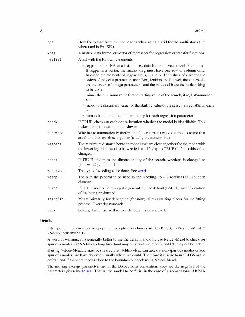
eps3 How far to start from the boundaries when using a grid for the multi-starts (i.e.when rand is FALSE.)

xreg A matrix, data frame, or vector of regressors for regression or transfer functions.

reglist A list with the following elements:

• regpar - either NA or a list, matrix, data frame, or vector with 3 columns.If regpar is a vector, the matrix xreg must have one row or column only.In order, the elements of regpar are: r, s, and b. The values of r are the theorders of the delta parameters as in Box, Jenkins and Reinsel, the values of sare the orders of omega parameters, and the values of b are the backshiftingto be done.

• minn - the minimum value for the starting value of the search, if reglist$numeach> 1.

• maxx - the maximum value for the starting value of the search, if reglist$numeach> 1.

• numeach - the number of starts to try for each regression parameter.

check If TRUE, checks at each optim iteration whether the model is identifiable. Thismakes the optimization much slower.

autoweed Whether to automatically (before the fit is returned) weed out modes found thatare found that are close together (usually the same point.)

weedeps The maximum distance between modes that are close together for the mode withthe lower log-likelihood to be weeded out. If adapt is TRUE (default) this valuechanges.

adapt If TRUE, if dim is the dimensionality of the search, weedeps is changed to(1 + weedeps)dim − 1.

weedtype The type of weeding to be done. See weed.

weedp The p in the p-norm to be used in the weeding. p = 2 (default) is Euclideandistance.

quiet If TRUE, no auxiliary output is generated. The default (FALSE) has informationof fits being proformed.

startfit Meant primarily for debugging (for now), allows starting places for the fittingprocess. Overrides numeach.

back Setting this to true will restore the defaults in numeach.

Details

Fits by direct optimization using optim. The optimizer choices are: 0 - BFGS; 1 - Nealder-Mead; 2- SANN; otherwise CG.

A word of warning: it is generally better to use the default, and only use Nelder-Mead to check forspurious modes. SANN takes a long time (and may only find one mode), and CG may not be stable.

If using Nelder-Mead, it must be stressed that Nelder-Mead can take out non-spurious modes or addspurious modes: we have checked visually where we could. Therefore it is wise to use BFGS as thedefault and if there are modes close to the boundaries, check using Nelder-Mead.

The moving average parameters are in the Box-Jenkins convention: they are the negative of theparameters given by arima. That is, the model to be fit is, in the case of a non-seasonal ARIMA

arfima 9

model, phi(B) (1-B)^d z[t] = theta(B) a[t], where phi(B) = 1 - phi(1) B - ... - phi(p) B^p and theta(B)= 1 - theta(1) B - ... - theta(q) B^q.

For the useC parameter, a "0" means no C is used; a "1" means C is only used to compute thelog-likelihood, but not the theoretical autocovariance function (tacvf); a "2" means that C is used tocompute the tacvf and not the log-likelihood; and a "3" means C is used to compute everything.

Value

An object of class "arfima". In it, full information on the fit is given, though not printed underthe print.arfima method. The phis are the AR parameters, and the thetas are the MA parameters.Residuals, regression residuals, etc., are all available, along with the parameter values and standarderrors. Note that the muHat returned in the arfima object is of the differenced series, if differencingis applied.

Note that if multiple modes are found, they are listed in order of log-likelihood value.

Author(s)


References

McLeod, A. I., Yu, H. and Krougly, Z. L. (2007) Algorithms for Linear Time Series Analysis: WithR Package Journal of Statistical Software, Vol. 23, Issue 5


P. Borwein (1995) An efficient algorithm for Riemann Zeta function Canadian Math. Soc. Conf.Proc., 27, pp. 29-34.

See Also

arfima.sim, SeriesJ, arfima-package

Examples

set.seed(8564)sim <- arfima.sim(1000, model = list(phi = c(0.2, 0.1),dfrac = 0.4, theta = 0.9))fit <- arfima(sim, order = c(2, 0, 1), back=T)

fit

data(tmpyr)

fit <- arfima(tmpyr, order = c(1, 0, 1), numeach = c(3, 3))fit

plot(tacvf(fit), maxlag = 30, tacf = TRUE)

data(SeriesJ)

10 arfima.sim

attach(SeriesJ)

fitTF <- arfima(YJ, order= c(2, 0, 0), xreg = XJ, reglist =list(regpar = c(2, 2, 3)), lmodel = "n")fitTF

detach(SeriesJ)

arfima.sim Simulate an ARFIMA time series.

Description

This function simulates an long memory ARIMA time series, with one of fractionally differencedwhite noise (FDWN), fractional Gaussian noise (FGN), power-law autocovariance (PLA) noise, orshort memory noise and possibly seasonal effects.

Usage

arfima.sim(n, model = list(phi = numeric(0), theta = numeric(0), dint = 0,dfrac = numeric(0), H = numeric(0), alpha = numeric(0), seasonal = list(phi =numeric(0), theta = numeric(0), dint = 0, period = numeric(0), dfrac =numeric(0), H = numeric(0), alpha = numeric(0))), useC = 3, sigma2 = 1,rand.gen = rnorm, muHat = 0, zinit = NULL, innov = NULL, ...)

Arguments

n The number of points to be generated.

model The model to be simulated from. The phi and theta arguments should be vectorswith the values of the AR and MA parameters. Note that Box-Jenkins notationis used for the MA parameters: see the "Details" section of arfima. The dintargument indicates how much differencing should be required to make the pro-cess stationary. The dfrac, H, and alpha arguments are FDWN, FGN and PLAvalues respectively; note that only one (or none) of these can have a value, or anerror is returned. The seasonal argument is a list, with the same parameters, anda period, as the model argument. Note that with a seasonal model, we can havemixing of FDWN/FGN/HD noise: one in the non-seasonal part, and the other inthe seasonal part.

useC How much interfaced C code to use: an integer between 0 and 3. The value 3 isstrongly recommended. See the "Details" section of arfima.

sigma2 The desired variance for the innovations of the series.

rand.gen The distribution of the innovations. Any distribution recognized by R is possible

muHat The theoretical mean of the series before integration (if integer integration isdone)

arfima.sim 11

zinit Used for prediction; not meant to be used directly. This allows a start of a timeseries to be specified before inverse differencing (integration) is applied.

innov Used for prediction; not meant to be used directly. This allows for the use ofgiven innovations instead of ones provided by rand.gen.

... Other parameters passed to the random variate generator; currently not used.

Details

A suitably defined stationary series is generated, and if either of the dints (non-seasonal or seasonal)are greater than zero, the series is integrated (inverse-differenced) with zinit equalling a suitableamount of 0s if not supplied. Then a suitable amount of points are taken out of the beginning of theseries (i.e. dint + period * seasonal dint = the length of zinit) to obtain a series of length n. Thestationary series is generated by calculating the theoretical autovariance function and using it, alongwith the innovations to generate a series as in McLeod et. al. (2007).

Value

A sample from a multivariate normal distribution that has a covariance structure defined by theautocovariances generated for given parameters. The sample acts like a time series with the givenparameters.

Author(s)


References

McLeod, A. I., Yu, H. and Krougly, Z. L. (2007) Algorithms for Linear Time Series Analysis: WithR Package Journal of Statistical Software, Vol. 23, Issue 5



See Also

arfima

Examples

set.seed(6533)sim <- arfima.sim(1000, model = list(phi = .2, dfrac = .3, dint = 2))

fit <- arfima(sim, order = c(1, 2, 0))fit

12 arfima0

arfima0 Exact MLE for ARFIMA

Description

The time series is corrected for the sample mean and then exact MLE is used for the other param-eters. This is a simplified version of the arfima() function that may be useful in simulations andbootstrapping.

Usage

arfima0(z, order = c(0, 0, 0), lmodel = c("FD", "FGN", "PLA", "NONE"))

Arguments

z time seriesorder (p,d,q) where p=order AR, d=regular difference, q=order MAlmodel type of long-memory component: FD, FGN, PLA or NONE

Details

The sample mean is asymptotically efficient.

Value

list with components:

bHat transformed optimal parametersalphaHat estimate of alphaHHat estimate of HdHat estimate of dphiHat estimate of phithetaHat estimate of thetawLL optimized value of Whittle approximate log-likelihoodLL corresponding exact log-likelihoodconvergence convergence indicator

Author(s)

JQ (Justin) Veenstra and A. I. McLeod

Examples

z <- rnorm(100)arfima0(z, lmodel="FGN")

arfimachanges 13

arfimachanges Prints changes to the package since the last update. Started in 1.4-0

Description

Prints changes to the package since the last update. Started in 1.4-0

Usage

arfimachanges()

ARToPacf Converts AR/MA coefficients from operator space to the PACF space

Description

Converts AR/MA coefficients from operator space to the PACF box-space; usually for internal use

Usage

ARToPacf(phi)

Arguments

phi The AR/MA coefficients in operator space

Value

The AR/MA coefficients in the PACF space

Author(s)

A. I. McLeod

References

Barndorff-Nielsen O. E., Schou G. (1973). "On the parametrization of autoregressive models bypartial autocorrelations." Journal of Multivariate Analysis, 3, 408-419

McLeod A. I., Zhang Y (2006). "Partial autocorrelation parameterization for subset autore- gres-sion." Journal of Time Series Analysis, 27(4), 599-612

14 bestModes

bestModes Finds the best modes of an arfima fit.

Description

Finds the best modes of an arfima fit with respect to log-likelihood.

Usage

bestModes(object, bestn)

Arguments

object An object of class "arfima".

bestn The top number of modes to keep with respect to the log-likelihood.

Details

This is the easiest way to remove modes with lower log-likelihoods.

Value

The bestn "best" modes.

Author(s)


See Also

arfima

Examples

set.seed(8765)sim <- arfima.sim(1000, model = list(phi = 0.4, theta = 0.9, dfrac = 0.4))fit <- arfima(sim, order = c(1, 0, 1), back=T)fitfit <- bestModes(fit, 2)fit

coef.arfima 15

coef.arfima Extract Model Coefficients

Description

Extracts the coefficients from a arfima fit.

Usage

## S3 method for class 'arfima'coef(object, tpacf = FALSE, digits = max(4,getOption("digits") - 3), ...)

Arguments

object A fitted arfima object.

tpacf If TRUE, the (ARMA) coefficients are in the transformed PACF space.

digits The number of digits to print

... Other optional arguments. Currently not used.

Value

A matrix of coefficients. The rows are for the modes, and the columns are for the model variables.

Author(s)


Examples


fitcoef(fit)

16 distance

distance The distance between modes of an arfima fit.

Description

The distance between modes of an arfima fit.

Usage

distance(ans, p = 2, digits = 4)

Arguments

ans An object of class "arfima".

p The p in the p-norm to be used.

digits The number of digits to print.

Value

A list of two data frames: one with distances in operator space, the second with distances in thetransformed (PACF) space.

Author(s)

JQ (Justin) Veensta

References


Examples


fit

distance(fit)

fitted.arfima 17

fitted.arfima Extract Model Fitted Values

Description

Extract fitted values from an arfima object.

Usage

## S3 method for class 'arfima'fitted(object, ...)

Arguments

object A arfima object.

... Optional parameters. Currently not used.

Value

A list of vectors of fitted values, one for each mode.

Author(s)


References


See Also

arfima, resid.arfima

Examples


fit

resid <- resid(fit)par(mfrow = c(1, 3))fitted <- fitted(fit)plot(fitted[[1]], resid[[1]])plot(fitted[[2]], resid[[2]])plot(fitted[[3]], resid[[3]])

18 iARFIMA

par(mfrow = c(1, 1))

iARFIMA The Fisher information matrix of an ARFIMA process

Description

Computes the approximate or (almost) exact Fisher information matrix of an ARFIMA process

Usage

iARFIMA(phi = numeric(0), theta = numeric(0), phiseas = numeric(0),thetaseas = numeric(0), period = 0, dfrac = TRUE, dfs = FALSE,exact = TRUE)

Arguments

phi The autoregressive parameters in vector form.

theta The moving average parameters in vector form. See Details for differences fromarima.

phiseas The seasonal autoregressive parameters in vector form.

thetaseas The seasonal moving average parameters in vector form. See Details for differ-ences from arima.

period The periodicity of the seasonal components. Must be >= 2.

dfrac TRUE if we include the fractional d parameter, FALSE otherwise

dfs TRUE if we include the seasonal fractional d parameter, FALSE otherwise

exact If FALSE, calculate the approximate information matrix via psi-weights. Oth-erwise the (almost) exact information matrix will be calculated. See "Details".

Details

The matrices are calculated as outlined in Veenstra and McLeod (2012), which draws on manyreferences. The psi-weights approximation has a fixed maximum lag for the weights as 2048 (tobe changed to be adaptable.) The fractional difference(s) by AR/MA components have a fixedmaximum lag of 256, also to be changed. Thus the exact matrix has some approximation to it. Alsonote that the approximate method takes much longer than the "exact" one.

The moving average parameters are in the Box-Jenkins convention: they are the negative of theparameters given by arima.

Value

The information matrix of the model.

IdentInvertQ 19

Author(s)


References


See Also

IdentInvertQ

Examples

tick <- proc.time()exactI <- iARFIMA(phi = c(.4, -.2), theta = c(.7), phiseas = c(.8, -.4),d = TRUE, dfs = TRUE, period = 12)proc.time() - ticktick <- proc.time()approxI <- iARFIMA(phi = c(.4, -.2), theta = c(.7), phiseas = c(.8, -.4),d = TRUE, dfs = TRUE, period = 12, exact = FALSE)proc.time() - tickexactImax(abs(exactI - approxI))

IdentInvertQ Checks invertibility, stationarity, and identifiability of a given set ofparameters

Description

Computes whether a given long memory model is invertible, stationary, and identifiable.

Usage

IdentInvertQ(phi = numeric(0), theta = numeric(0), phiseas = numeric(0),thetaseas = numeric(0), dfrac = numeric(0), dfs = numeric(0),H = numeric(0), Hs = numeric(0), alpha = numeric(0),alphas = numeric(0), delta = numeric(0), period = 0, debug = FALSE,ident = TRUE)

20 IdentInvertQ

Arguments





dfrac The fractional differencing parameter.

dfs The seasonal fractional differencing parameter.

H The Hurst parameter for fractional Gaussian noise (FGN). Should not be mixedwith dfrac or alpha: see "Details".

Hs The Hurst parameter for seasonal fractional Gaussian noise (FGN). Should notbe mixed with dfs or alphas: see "Details".

alpha The decay parameter for power-law autocovariance (PLA) noise. Should not bemixed with dfrac or H: see "Details".

alphas The decay parameter for seasonal power-law autocovariance (PLA) noise. Shouldnot be mixed with dfs or Hs: see "Details".

delta The delta parameters for transfer functions.


debug When TRUE and model is not stationary/invertible or identifiable, prints somehelpful output.

ident Whether to test for identifiability.

Details

This function tests for identifiability via the information matrix of the ARFIMA process. Whetherthe process is stationary or invertible amounts to checking whether all the variables fall in correctranges.


If dfrac/H/alpha are mixed and/or dfs/Hs/alphas are mixed, an error will not be thrown, eventhough only one of these can drive the process at either level. Note also that the FGN or PLA haveno impact on the identifiability of the model, as information matrices containing these parameterscurrently do not have known closed form. These two parameters must be within their correct ranges(0<H<1 for FGN and 0 < alpha < 3 for PLA.)

Value

TRUE if the model is stationary, invertible and identifiable. FALSE otherwise.

Author(s)

Justin Veenstra

lARFIMA 21

References

McLeod, A.I. (1999) Necessary and sufficient condition for nonsingular Fisher information matrixin ARMA and fractional ARMA models The American Statistician 53, 71-72.

Veenstra, J. and McLeod, A. I. (2012, Submitted) Improved Algorithms for Fitting Long MemoryModels: With R Package

See Also

iARFIMA

Examples

IdentInvertQ(phi = 0.3, theta = 0.3)IdentInvertQ(phi = 1.2)

lARFIMA Exact log-likelihood of a long memory model

Description

Computes the exact log-likelihood of a long memory model with respect to a given time series.

Usage

lARFIMA(z, phi = numeric(0), theta = numeric(0), dfrac = numeric(0),phiseas = numeric(0), thetaseas = numeric(0), dfs = numeric(0),H = numeric(0), Hs = numeric(0), alpha = numeric(0),alphas = numeric(0), period = 0, useC = 3)

Arguments

z A vector or (univariate) time series object, assumed to be (weakly) stationary.








22 lARFIMA






Details

The log-likelihood is computed for the given series z and the parameters. If two or more of dfrac,H or alpha are present and/or two or more of dfs, Hs or alphas are present, an error will be thrown,as otherwise there is redundancy in the model. Note that non-seasonal and seasonal componentscan be of different types: for example, there can be seasonal FGN with FDWN at the non-seasonallevel.


For the useC parameter, a "0" means no C is used; a "1" means C is only used to compute thelog-likelihood, but not the theoretical autocovariance function (tacvf); a "2" means that C is used tocompute the tacvf and not the log-likelihood; and a "3" means C is used to compute everything.

Note that the time series is assumed to be stationary: this function does not do any differencing.

Value

The exact log-likelihood of the model given with respect to z, up to an additive constant.

Author(s)

Justin Veenstra

References

Box, G. E. P., Jenkins, G. M., and Reinsel, G. C. (2008) Time Series Analysis: Forecasting andControl. 4th Edition. John Wiley and Sons, Inc., New Jersey.


See Also

arfima

lARFIMAwTF

tacvfARFIMA

lARFIMAwTF 23

Examples

set.seed(3452)sim <- arfima.sim(1000, model = list(phi = c(0.3, -0.1)))lARFIMA(sim, phi = c(0.3, -0.1))

lARFIMAwTF Exact log-likelihood of a long memory model with a transfer functionmodel and series included

Description

Computes the exact log-likelihood of a long memory model with respect to a given time series aswell as a transfer fucntion model and series. This function is not meant to be used directly.

Usage

lARFIMAwTF(z, phi = numeric(0), theta = numeric(0), dfrac = numeric(0),phiseas = numeric(0), thetaseas = numeric(0), dfs = numeric(0),H = numeric(0), Hs = numeric(0), alpha = numeric(0),alphas = numeric(0), xr = numeric(0), r = numeric(0), s = numeric(0),b = numeric(0), delta = numeric(0), omega = numeric(0), period = 0,useC = 3, meanval = 0)

Arguments

z A vector or (univariate) time series object, assumed to be (weakly) stationary.











24 logLik.arfima

xr The regressors in vector form

r The order of the delta(s)

s The order of the omegas(s)

b The backshifting to be done

delta Transfer function parameters as in Box, Jenkins, and Reinsel. Corresponds tothe "autoregressive" part of the dynamic regression.

omega Transfer function parameters as in Box, Jenkins, and Reinsel. Corresponds tothe "moving average" part of the dynamic regression: note that omega_0 is notrestricted to 1. See "Details" for issues.



meanval If the mean is to be estimated dynamically, the mean.

Details

Once again, this function should not be used externally.

Value

A log-likelihood value

Author(s)

Justin Veenstra

References


logLik.arfima Extract Log-Likelihood Values

Description

Extracts log-likelihood values from a arfima fit.

Usage

## S3 method for class 'arfima'logLik(object, ...)

Arguments

object A fitted arfima object

... Optional arguments not currently used.

PacfToAR 25

Details

Uses the function DLLoglikelihood from the package ltsa. The log-likelihoods returned are exactup to an additive constant.

Value

A vector of log-likelihoods, one for each mode, is returned, along with the degrees of freedom.

Author(s)


References


See Also

AIC.arfima

PacfToAR Converts AR/MA coefficients from the PACF space to operator space

Description

Converts AR/MA coefficients from PACF box-space to operator space; usually for internal use

Usage

PacfToAR(pi)

Arguments

pi The AR/MA coefficients in PACF box-space

Value

The AR/MA coefficients in operator space.

Author(s)

A. I. McLeod

References

Barndorff-Nielsen O. E., Schou G. (1973). "On the parametrization of autoregressive models bypartial autocorrelations." Journal of Multivariate Analysis, 3, 408-419

McLeod A. I. , Zhang Y (2006). "Partial autocorrelation parameterization for subset autore- gres-sion." Journal of Time Series Analysis, 27(4), 599-612

26 plot.predarfima

plot.predarfima Plots the original time series, the predictions, and the prediction in-tervals for a predarfima object.

Description

This function takes a predarfima object generated by predict.arfima and plots all of the infor-mation contained in it. The colour code is as follows:

Usage

## S3 method for class 'predarfima'plot(x, xlab = NULL, ylab = NULL, main = NULL,ylim = NULL, numback = 5, xlim = NULL, ...)

Arguments

x A predarfima object

xlab Optional

ylab Optional

main Optional

ylim Optional

numback The number of last values of the original series to plot defined by the user. Thedefault is five

xlim Optional

... Currently not used

Details

grey: exact prediction red: exact prediction intervals (PIs) orange: limiting PIs

See predict.arfima.

Value

None. Generates a plot

Author(s)


References


plot.tacvf 27

See Also

predict.arfima, print.predarfima

Examples

set.seed(82365)sim <- arfima.sim(1000, model = list(dfrac = 0.4, theta=0.9, dint = 1))fit <- arfima(sim, order = c(0, 1, 1), back=T)fitpred <- predict(fit, n.ahead = 5)predplot(pred)#Let's look at more contextplot(pred, numback = 50)

plot.tacvf Plots the output from a call to tacvf

Description

Plots the theoretical autocovariance functions of the modes for a fitted arfima object

Usage

## S3 method for class 'tacvf'plot(x, type = "o", pch = 20, xlab = NULL, ylab = NULL,main = NULL, xlim = NULL, ylim = NULL, tacf = FALSE, maxlag = NULL,lag0 = !tacf, ...)

Arguments

x A tacvf object from a call to said function

type See plot. The default is recommended for short maxlag

pch See plot

xlab See plot

ylab See plot

main See plot

xlim See plot

ylim See plot

tacf If TRUE, plots the theoretical autocorellations instead

maxlag The maximum lag for the plot

28 predict.arfima

lag0 Whether or not to plot lag 0 of the tacvfs/tacfs. Default !tacf. Used bytacfplot.


Details

Only plots up to nine tacvfs. It is highly recommended that the arfima object be weeded beforecalling tacvf

Value

None. There is a plot as output.

Author(s)


References


See Also

tacvf

Examples

set.seed(1234)sim <- arfima.sim(1000, model = list(theta = 0.99, dfrac = 0.49))fit <- arfima(sim, order = c(0, 0, 1))plot(tacvf(fit))plot(tacvf(fit), tacf = TRUE)

predict.arfima Predicts from a fitted object.

Description

Performs prediction of a fitted arfima object. Includes prediction for each mode and exact andlimiting prediction error standard deviations. NOTE: the standard errors in beta are currentlynot taken into account in the prediction intervals shown. This will be updated as soon aspossible.

predict.arfima 29

Usage

## S3 method for class 'arfima'predict(object, n.ahead = 1, prop.use = "default",newxreg = NULL, predint = 0.95, exact = c("default", T, F),setmuhat0 = FALSE, cpus = 1, trend = NULL, n.use = NULL,xreg = NULL, ...)

Arguments


n.ahead The number of steps ahead to predict

prop.use The proportion (between 0 and 1) or percentage (between >1 and 100) of datapoints to use for prediction. Defaults to the string "default", which sets thenumber of data points n.use to the minimum of the series length and 1000.Overriden by n.use.

newxreg If a regression fit, the new regressors

predint The percentile to use for prediction intervals assuming normal deviations.

exact Controls whether exact (based on the theoretical autocovariance matrix) pre-diction variances are calculated (which is recommended), as well as whether theexact prediction formula is used when the process is differenced (which can takea fair amount of time if the length of the series used to predict is large). Defaultsto the string "default", which is TRUE for the first and FALSE for the second. ABoolean value (TRUE or FALSE) will set both to this value.

setmuhat0 Experimental. Sets muhat equal to zero

cpus The number of CPUs to use for prediction. Currently not implemented

trend An optional vector the length of n.ahead or longer to add to the predictions

n.use Directly set the number mentioned in prop.use.

xreg Alias for newxreg

... Optional arguments. Currently not used

Value

A list of lists, ceiling(prop.use * n)one for each mode with relavent details about the prediction

Author(s)


References


See Also

arfima, plot.predarfima, print.predarfima

30 print.arfima

Examples

set.seed(82365)sim <- arfima.sim(1000, model = list(dfrac = 0.4, theta=0.9, dint = 1))fit <- arfima(sim, order = c(0, 1, 1), back=T)fitpred <- predict(fit, n.ahead = 5)predplot(pred, numback=50)#Predictions aren't really different due to the#series. Let's see what happens when we regress!

set.seed(23524)#Forecast 5 ahead as before#Note that we need to integrate the regressors, since time series regression#usually assumes that regressors are of the same order as the series.n.fore <- 5X <- matrix(rnorm(3000+3*n.fore), ncol = 3)X <- apply(X, 2, cumsum)Xnew <- X[1001:1005,]X <- X[1:1000,]beta <- matrix(c(2, -.4, 6), ncol = 1)simX <- sim + as.vector(X%*%beta)fitX <- arfima(simX, order = c(0, 1, 1), xreg = X, back=T)fitX#Let's compare predictions.predX <- predict(fitX, n.ahead = n.fore, xreg = Xnew)predXplot(predX, numback = 50)#With the mode we know is really there, it looks better.fitX <- removeMode(fitX, 2)predXnew <- predict(fitX, n.ahead = n.fore, xreg = Xnew)predXnewplot(predXnew, numback=50)

#

print.arfima Prints a Fitted Object

Description

Prints a fitted arfima object’s relevant details

Usage

## S3 method for class 'arfima'print(x, digits = max(6, getOption("digits") - 3), ...)

print.predarfima 31

Arguments

x A fitted arfima object


... Optional arguments. See print.

Value

The object is returned invisibly

Author(s)


References


print.predarfima Prints predictions and prediction intervals

Description

Prints the output of predict on an arfima object

Usage

## S3 method for class 'predarfima'print(x, digits = max(6, getOption("digits") - 3), ...)

Arguments

x An object of class "predarfima"



Details

Prints all the relavent output of the prediction function of the arfima package

Value

x is returned invisibly

Author(s)


32 print.summary.arfima

See Also

arfima, predict.arfima, predict, plot.predarfima

Examples

set.seed(82365)sim <- arfima.sim(1000, model = list(dfrac = 0.4, theta=0.9, dint = 1))fit <- arfima(sim, order = c(0, 1, 1), back=T)fitpred <- predict(fit, n.ahead = 5)predplot(pred)

print.summary.arfima Prints the output of a call to summary on an arfima object

Description

Prints the output of a call to summary on an arfima object

Usage

## S3 method for class 'summary.arfima'print(x, digits = max(6, getOption("digits") - 3),signif.stars = getOption("show.signif.stars"), ...)

Arguments

x A summary.arfima object


signif.stars Whether to print stars on significant output


Value

Returns the object x invisibly

Author(s)


References


print.tacvf 33

See Also

arfima, print.arfima, summary.arfima, print

Examples

set.seed(54678)sim <- arfima.sim(1000, model = list(phi = 0.9, H = 0.3))fit <- arfima(sim, order = c(1, 0, 0), lmodel = "g", back=T)summary(fit)

print.tacvf Prints a tacvf object.

Description

Prints the output of a call to tacvf on an arfima object

Usage

## S3 method for class 'tacvf'print(x, ...)

Arguments

x The tacvf object.

... Optional arguments. See print.

Value

The object is returned invisibly

Author(s)


See Also

tacvf, plot.tacvf

34 removeMode

removeMode Removes a mode from an arfima fit.

Description

This function is useful if one suspects a mode is spurious and does not want to call the weedfunction.

Usage

removeMode(object, num)

Arguments

object An object of class "arfima".

num The number of the mode as in the printed value of the object.

Value

The original object with the mode removed.

Author(s)


See Also

arfima

Examples

set.seed(8765)sim <- arfima.sim(1000, model = list(phi = 0.4, theta = 0.9, dfrac = 0.4))fit <- arfima(sim, order = c(1, 0, 1), back=T)fitfit <- removeMode(fit, 3)fit

residuals.arfima 35

residuals.arfima Extract the Residuals of a Fitted Object

Description

Extracts the residuals or regression residuals from a fitted arfima object

Usage

## S3 method for class 'arfima'residuals(object, reg = FALSE, ...)

Arguments


reg Whether to extract the regression residuals instead. If TRUE, throws an error ifno regression was done.

... Optional parameters. Currently not used.

Value

A list of vectors of residuals, one for each mode.

Author(s)


References


See Also

arfima, fitted.arfima

Examples


fit

resid <- resid(fit)par(mfrow = c(1, 3))plot(resid[[1]])

36 SeriesJ

plot(resid[[2]])plot(resid[[3]])fitted <- fitted(fit)plot(fitted[[1]], resid[[1]])plot(fitted[[2]], resid[[2]])plot(fitted[[3]], resid[[3]])par(mfrow = c(1, 1))

SeriesJ Series J, Gas Furnace Data

Description

Gas furnace data, sampling interval 9 seconds; observations for 296 pairs of data points.

Format

List with ts objects XJ and YJ.

Details

XJ is input gas rate in cubic feet per minute, YJ is percentage carbon dioxide (CO2) in outlet gas.X is the regressor.

Box, Jenkins, and Reinsel (2008) fit an AR(2) to YJ, with transfer function specifications r = 2, s =2, and b = 3, regressing on XJ. Our package agrees with their results.

Source

Box, Jenkins and Reinsel(2008). Time Series Analysis: Forecasting and Control.

References

Box, G. E. P., Jenkins, G. M., and Reinsel, G. C. (2008) Time Series Analysis: Forecasting andControl. 4th Edition. John Wiley and Sons, Inc., New Jersey.

Veenstra, J. and McLeod, A. I. (Working Paper). The arfima R package: Exact Methods for Hyper-bolic Decay Time Series

Examples

data(SeriesJ)attach(SeriesJ)

fitTF <- arfima(YJ, order= c(2, 0, 0), xreg = XJ, reglist =list(regpar = c(2, 2, 3)), lmodel = "n")fitTF ## agrees fairly closely with Box et. al.

summary.arfima 37

detach(SeriesJ)

summary.arfima Extensive Summary of an Object

Description

Provides a very comprehensive summary of a fitted arfima object. Includes correlation and co-variance matrices (observed and expected), the Fisher Information matrix of those parameters forwhich it is defined, and more, for each mode.

Usage

## S3 method for class 'arfima'summary(object, digits = max(4, getOption("digits") - 3),...)

Arguments



... Optional arguments, currently not used.

Value

A list of lists (one for each mode) of all relevant information about the fit that can be passed toprint.summary.arfima.

Author(s)


References


See Also

arfima, iARFIMA, vcov.arfima

38 tacfplot

Examples

data(tmpyr)

fit <- arfima(tmpyr, order = c(1, 0, 1), back=T)fit

summary(fit)

tacfplot Plots the theoretical autocorralation functions (tacfs) of one or morefits.

Description

Plots the theoretical autocorralation functions (tacfs) of one or more fits.

Usage

tacfplot(fits = list(), modes = "all", xlab = NULL, ylab = NULL,main = NULL, xlim = NULL, ylim = NULL, maxlag = 20, lag0 = FALSE,...)

Arguments

fits A list of objects of class "arfima".

modes Either "all" or a vector of the same length as fits for which the tacfs will beploted.

xlab Optional. Usually better to be generated by the function.

ylab Optional. Usually better to be generated by the function.

main Optional. Usually better to be generated by the function.

xlim Optional. Usually better to be generated by the function.

ylim Optional. Usually better to be generated by the function.

maxlag Optional. Used to limit the length of tacfs. Highly recommended to be a valuefrom 20 - 50.

lag0 Whether or not the lag 0 tacf should be printed. Since this is always 1 for alltacfs, recommended to be TRUE. It is easier to see the shape of the tacfs.

... Optional. Currently not used.

Value

NULL. However, there is a plot output.

tacvf 39

Author(s)


References


See Also

tacvf, plot.tacvf

Examples

set.seed(34577)sim <- arfima.sim(500, model = list(theta = 0.9, phi = 0.5, dfrac = 0.4))fit1 <- arfima(sim, order = c(1, 0, 1), cpus = 2, back=T)fit2 <- arfima(sim, order = c(1, 0, 1), cpus = 2, lmodel = "g", back=T)fit3 <- arfima(sim, order = c(1, 0, 1), cpus = 2, lmodel = "h", back=T)fit1fit2fit3tacfplot(fits = list(fit1, fit2, fit3), maxlag = 30)

tacvf Extracts the tacvfs of a fitted object

Description

Extracts the theoretical autocovariance functions (tacvfs) from a fitted arfima or one of its modes(an ARFIMA) object.

Usage

tacvf(obj, xmaxlag = 0, forPred = FALSE, n.ahead = 0, nuse = -1, ...)

Arguments

obj An object of class "arfima" or "ARFIMA". The latter class is a mode of theformer.

xmaxlag The number of extra points to be added on to the end. That is, if the originalseries has length 300, and xmaxlag = 5, the tacvfs will go from lag 0 to lag 304.

forPred Should only be TRUE from a call to predict.arfima.n.ahead Only used internally.nuse Only used internally.... Optional arguments, currently not used.

40 tacvfARFIMA

Value

A list of tacvfs, one for each mode, the length of the time series.

Author(s)


References


See Also

plot.tacvf, print.tacvf, tacfplot, arfima

tacvfARFIMA The theoretical autocovariance function of a long memory process.

Description

Calculates the tacvf of a mixed long memory-ARMA (with posible seasonal components). Com-bines long memory and ARMA (and non-seasonal and seasonal) parts via convolution.

Usage

tacvfARFIMA(phi = numeric(0), theta = numeric(0), dfrac = numeric(0),phiseas = numeric(0), thetaseas = numeric(0), dfs = numeric(0),H = numeric(0), Hs = numeric(0), alpha = numeric(0),alphas = numeric(0), period = 0, maxlag, useCt = T, sigma2 = 1)

Arguments









tacvfARFIMA 41




maxlag The number of terms to compute: technically the output sequence is from lags0 to maxlag, so there are maxlag + 1 terms.

useCt Whether or not to use C to compute the (parts of the) tacvf.

sigma2 Used in arfima.sim: determines the value of the innovation variance. The tacvfsequence is multiplied by this value.

Details

The log-likelihood is computed for the given series z and the parameters. If two or more of dfrac,H or alpha are present and/or two or more of dfs, Hs or alphas are present, an error will be thrown,as otherwise there is redundancy in the model. Note that non-seasonal and seasonal componentscan be of different types: for example, there can be seasonal FGN with FDWN at the non-seasonallevel.


Value

A sequence of length maxlag + 1 (lags 0 to maxlag) of the tacvf of the given process.

Author(s)

JQ (Justin) Veenstra and A. I. McLeod

References



Examples

t1 <- tacvfARFIMA(phi = c(0.2, 0.1), theta = 0.4, dfrac = 0.3, maxlag = 30)t2 <- tacvfARFIMA(phi = c(0.2, 0.1), theta = 0.4, H = 0.8, maxlag = 30)t3 <- tacvfARFIMA(phi = c(0.2, 0.1), theta = 0.4, alpha = 0.4, maxlag = 30)plot(t1, type = "o", col = "blue", pch = 20)lines(t2, type = "o", col = "red", pch = 20)lines(t3, type = "o", col = "purple", pch = 20) #they decay at about the same rate

42 tmpyr

tmpyr Temperature Data

Description

Central England mean yearly temperatures from 1659 to 1976

Format

A ts tmpyr

Details

Hosking notes that while the ARFIMA(1, d, 1) has a lower AIC, it is not much lower than the AICof the ARFIMA(1, d, 0).

Bhansali and Kobozka find: muHat = 9.14, d = 0.28, phi = -0.77, and theta = -0.66 for theARFIMA(1, d, 1), which is close to our result, although our result reveals trimodality if numeach islarge enough. The third mode is close to Hosking’s fit of an ARMA(1, 1) to these data, while thesecond is very antipersistent.

Our package gives a very close result to Hosking for the ARFIMA(1, d, 0) case, although there isalso a second mode. Given how close it is to the boundary, it may or may not be spurious. A checkwith dmean = FALSE shows that it is not the optimized mean giving a spurious mode.

If, however, we use whichopt = 1, we only have one mode. Note that Nelder-Mead sometimesdoes take out non-spurious modes, or add spurious modes to the surface.

Source

http://www.metoffice.gov.uk/hadobs/hadcet/

References

Parker, D.E., Legg, T.P., and Folland, C.K. (1992). A new daily Central England TemperatureSeries, 1772-1991. Int. J. Clim., Vol 12, pp 317-342

Manley,G. (1974). Central England Temperatures: monthly means 1659 to 1973. Q.J.R. Meteorol.Soc., Vol 100, pp 389-405.

Hosking, J. R. M. (1984). Modeling persistence in hydrological time series using fractional differ-encing, Water Resour. Res., 20(12)

Bhansali, R. J. and Koboszka, P. S. (2003) Prediction of Long-Memory Time Series In Doukhan,P., Oppenheim, G. and Taqqu, M. S. (Eds) Theory and Applications of Long-Range Dependence(pp355-368) Birkhauser Boston Inc.


http://www.metoffice.gov.uk/hadobs/hadcet/

vcov.arfima 43

Examples

data(tmpyr)

fit <- arfima(tmpyr, order = c(1, 0, 1), numeach = c(3, 3), dmean = TRUE, back=T)fit##suspect that fourth mode may be spurious, even though not close to a boundary##may be an induced mode from the optimization of the mean

fit <- arfima(tmpyr, order = c(1, 0, 1), numeach = c(3, 3), dmean = FALSE, back=T)fit

##perhaps so

plot(tacvf(fit), maxlag = 30, tacf = TRUE)

fit1 <- arfima(tmpyr, order = c(1, 0, 0), dmean = TRUE, back=T)fit1

fit2 <- arfima(tmpyr, order = c(1, 0, 0), dmean = FALSE, back=T)fit2 ##still bimodal. Second mode may or may not be spurious.

fit3 <- arfima(tmpyr, order = c(1, 0, 0), dmean = FALSE, whichopt = 1, numeach = c(3, 3))fit3 ##Unimodal. So the second mode was likely spurious.

plot(tacvf(fit2), maxlag = 30, tacf = TRUE)##maybe not spurious. Hard to tell without visualizing the surface.

##compare to plotted tacf of fit1: looks alikeplot(tacvf(fit1), maxlag = 30, tacf = TRUE)

tacfplot(list(fit1, fit2))

vcov.arfima Extracts the Variance-Covariance Matrix

Description

Extracts the variance-covariance matrices (one or two for each mode) from a fitted arfima object.

Usage

## S3 method for class 'arfima'vcov(object, type = c("b", "o", "e"), cor = FALSE,digits = max(4, getOption("digits") - 3), tapprox = FALSE, summ = FALSE,...)

44 vcov.arfima

Arguments


type Which type of covariance matrix to return: "o" is the observed matrix (fromsolving the Hessian), "e" is the expected matrix (from solving the informationmatrix), and "b" is both.

cor Whether or not the correlation matrix should be returned instead.

digits The number of digits to print.

tapprox Whether or not to use an approximation to find the expected matrix. Highlyrecommended to be FALSE, as it takes much longer, and is an approximation.

summ Whether the call is from the summary.arfima function. Should not be usedexcept internally.

... Optional arguments, currently not used.

Value

A list of lists (one for each mode) with components observed and/or expected.

Author(s)


References


See Also

summary.arfima, arfima

Examples

set.seed(1234)sim <- arfima.sim(1000, model = list(dfrac = 0.4, phi = .8, theta = -0.5))fit1 <- arfima(sim, order = c(1, 0, 1), back=T)fit2 <- arfima(sim, order = c(1, 0, 1), lmodel = "g", back=T)fit3 <- arfima(sim, order = c(1, 0, 1), lmodel = "h", back=T)fit1fit2fit3vcov(fit1)vcov(fit2)vcov(fit2)

weed 45

weed Weeds out fits from a call to arfima that are too close to each other.

Description

Weeds out fits from a call to arfima that are too close to each other.

Usage

weed(ans, type = c("A", "P", "B", "N"), walls = FALSE, eps2 = 0.025,eps3 = 0.01, adapt = TRUE, pn = 2)

Arguments

ans The result from a call to arfima.

type The space to perform the weeding in. "A" is for operating parameters. "P" is inthe PACF space. "B" performs weeding in both. "N" performs no weeding andis only used internally.

walls If more than one mode is on a wall in the PACF space, all modes but the onewith the highest log-likelihood on the same wall are deleted.

eps2 The maximum distance between modes that are close together for the mode withthe lower log-likelihood to be weeded out. If adapt is TRUE (default) this valuechanges.

eps3 The minimum distance from a wall for a secondary mode to be weeded out, ifwalls are TRUE.

adapt If TRUE, if dim is the dimensionality of the search, eps2 is changed to (1 +eps2)dim − 1.

pn The p in the p-norm to be used in the weeding. p = 2 (default) is Euclideandistance.

Value

An object of class "arfima" with modes possibly weeded out.

Author(s)


See Also

arfima, distance

46 weed

Examples

set.seed(1234)sim <- arfima.sim(1000, model = list(theta = 0.9, dfrac = 0.4))fit <- arfima(sim, order = c(0, 0, 1), autoweed = FALSE, back=T)fitdistance(fit)fit1 <- weed(fit)fit1distance(fit1)

Index

∗Topic datasetsSeriesJ, 36tmpyr, 42

∗Topic fitarfima.sim, 10

∗Topic packagearfima-package, 2

∗Topic tsAIC.arfima, 5arfima, 6arfima.sim, 10arfima0, 12ARToPacf, 13bestModes, 14coef.arfima, 15distance, 16fitted.arfima, 17iARFIMA, 18IdentInvertQ, 19lARFIMA, 21lARFIMAwTF, 23logLik.arfima, 24PacfToAR, 25plot.predarfima, 26plot.tacvf, 27predict.arfima, 28print.arfima, 30print.predarfima, 31print.summary.arfima, 32print.tacvf, 33removeMode, 34residuals.arfima, 35summary.arfima, 37tacfplot, 38tacvf, 39tacvfARFIMA, 40vcov.arfima, 43weed, 45

AIC, 5

AIC.arfima, 3, 5, 25arfima, 3, 6, 10, 11, 14, 17, 22, 29, 32–35, 37,

40, 44, 45arfima-package, 2arfima.sim, 3, 9, 10, 41arfima0, 3, 12arfimachanges, 13arima, 7, 8, 18, 20–23, 40, 41ARToPacf, 13

bestModes, 14BIC (AIC.arfima), 5BIC.arfima, 3

coef.arfima, 3, 15

distance, 3, 16, 45

fitted.arfima, 3, 17, 35

iARFIMA, 3, 18, 21, 37IdentInvertQ, 3, 19, 19

lARFIMA, 3, 21lARFIMAwTF, 3, 22, 23logLik.arfima, 3, 24ltsa, 25

PacfToAR, 25plot, 27plot.predarfima, 3, 26, 29, 32plot.tacvf, 3, 27, 33, 39, 40predict, 32predict.arfima, 3, 26, 27, 28, 32print, 31, 33print.arfima, 3, 30, 33print.predarfima, 3, 27, 29, 31print.summary.arfima, 32print.tacvf, 3, 33, 40

removeMode, 3, 34

47

48 INDEX

resid.arfima, 17resid.arfima (residuals.arfima), 35residuals.arfima, 3, 35

SeriesJ, 3, 9, 36summary.arfima, 3, 33, 37, 44

tacfplot, 3, 28, 38, 40tacvf, 3, 28, 33, 39, 39tacvfARFIMA, 3, 22, 40tmpyr, 3, 42TrenchMean, 7

vcov.arfima, 3, 37, 43

weed, 3, 8, 45

Package ‘arﬁma’ - The Comprehensive R Archive Network have ﬁxed = list(phi = c(0, NA)). NA...

Documents

Transcript of Package ‘arﬁma’ - The Comprehensive R Archive Network have ﬁxed = list(phi = c(0, NA)). NA...