PAAR-2016

Fifth Workshop onPractical Aspects of Automated Reasoning

July 2, 2016

Affiliated with the 8th International Joint Conference on AutomatedReasoning (IJCAR 2016)

Coimbra, Portugal

http://cs.ru.nl/paar16/

Preface

This volume contains the papers presented at the Fifth Workshop on Practical Aspects of Automated Reasoning(PAAR-2016). The workshop was held on July 2, 2016, in Coimbra, Portugal, in association with the EighthInternational Joint Conference on Automated Reasoning (IJCAR-2016).

PAAR provides a forum for developers of automated reasoning tools to discuss and compare different im-plementation techniques, and for users to discuss and communicate their applications and requirements. Theworkshop brought together different groups to concentrate on practical aspects of the implementation and ap-plication of automated reasoning tools. It allowed researchers to present their work in progress, and to discussnew implementation techniques and applications.

Papers were solicited on topics that include all practical aspects of automated reasoning. More specifically,some suggested topics were:

• automated reasoning in propositional, first-order, higher-order and non-classical logics;

• implementation of provers (SAT, SMT, resolution, tableau, instantiation-based, rewriting, logical frame-works, etc);

• automated reasoning tools for all kinds of practical problems and applications;

• pragmatics of automated reasoning within proof assistants;

• practical experiences, usability aspects, feasibility studies;

• evaluation of implementation techniques and automated reasoning tools;

• performance aspects, benchmarking approaches;

• non-standard approaches to automated reasoning, non-standard forms of automated reasoning, new appli-cations;

• implementation techniques, optimization techniques, strategies and heuristics, fairness;

• support tools for prover development;

• system descriptions and demos.

We were particularly interested in contributions that help the community to understand how to build useful andpowerful reasoning systems in practice, and how to apply existing systems to real problems.

We received thirteen submissions. Each submission was reviewed by three program committee members. Dueto the quality of the submissions, eleven of them were accepted. The program committee also proposed to theremaining two submissions to present their work, as presentation only.

The workshop organizers would like to thank the authors and participants of the workshop, and the programcommittee and the reviewers for their effort.

We are very grateful to the IJCAR organizers for their support and for hosting the workshop, and are indebtedto the EasyChair team for the availability of the EasyChair Conference System.

June 2016 Pascal Fontaine, Stephan Schulz, Josef Urban

II

Program Committee

June Andronick (NICTA and University of New South Wales, Australia)Peter Baumgartner (NICTA/Australian National University, Australia)Christoph Benzmuller (Freie Universitat Berlin, Germany)Armin Bierre (Johannes Kepler University, Austria)Nikolaj Bjorner (Microsoft Research, USA)Simon Cruanes (Loria, INRIA, France)Hans de Nivelle (University of Wroclaw, Poland)Pascal Fontaine (Loria, INRIA, University of Lorraine, France), co-chairVijay Ganesh (University of Waterloo, Canada)Alberto Griggio (FBK-IRST, Italy)John Harrison (Intel, USA)Marijn Heule (The University of Texas at Austin, USA)Dejan Jovanovic (SRI International, USA)Yevgeny Kazakov (The University of Ulm, Germany)Chantal Keller (LRI, Universite Paris-Sud, France)Boris Konev (The University of Liverpool, UK)Konstantin Korovin (The University of Manchester, UK)Laura Kovacs (Chalmers University, Sweden)Jens Otten (University of Potsdam, Germany)Nicolas Peltier (CNRS - LIG, France)Ruzica Piskac (Yale University, USA)Giles Reger (The University of Manchester, UK)Andrew Reynolds (EPFL, Switzerland)Philipp Ruemmer (Uppsala University, Sweden)Uli Sattler (The University of Manchester, UK)Renate A. Schmidt (The University of Manchester, UK)Stephan Schulz (DHBW Stuttgart, Germany), co-chairGeoff Sutcliffe (University of Miami, USA)Josef Urban (Czech Technical University in Prague, Czech Republic), co-chairUwe Waldmann (MPI Saarbrucken, Germany)

External reviewersPeter BackemanMurphy BerzishChad BrownYizheng Zhao

III

Table of Contents

Efficient Instantiation Techniques in SMT (Work In Progress) . . . . . . . . . . . . . . . . . . . . . . . . . 1Haniel Barbosa

Alternative treatments of common binary relations in first-order automated reasoning . . . . . . . . . . . 11Koen Claessen and Ann Lilliestrom

No Choice: Reconstruction of First-order ATP Proofs without Skolem Functions . . . . . . . . . . . . . . 24Michael Farber and Cezary Kaliszyk

Deduction as a Service . . . . . . . . . . . . . . . . . . . . . . . . . . . . . . . . . . . . . . . . . . . . . . . 32Mohamed Hassona and Stephan Schulz

TH1: The TPTP Typed Higher-Order Form with Rank-1 Polymorphism . . . . . . . . . . . . . . . . . . . 41Cezary Kaliszyk, Geoff Sutcliffe and Florian Rabe

Prover-independent Axiom Selection for Automated Theorem Proving in Ontohub . . . . . . . . . . . . . 56Eugen Kuksa and Till Mossakowski

On Checking Kripke Models for Modal Logic K . . . . . . . . . . . . . . . . . . . . . . . . . . . . . . . . . 69Jean Marie Lagniez, Daniel Le Berre, Tiago de Lima and Valentin Montmirail

Towards a Substitution Tree Based Index for Higher-order Resolution Theorem Provers . . . . . . . . . . 82Tomer Libal and Alexander Steen

Ordered Resolution with Straight Dismatching Constraints . . . . . . . . . . . . . . . . . . . . . . . . . . 95Andreas Teucke and Christoph Weidenbach

A Saturation-based Algebraic Reasoner for ELQ . . . . . . . . . . . . . . . . . . . . . . . . . . . . . . . . 110Jelena Vlasenko, Maryam Daryalal, Volker Haarslev and Brigitte Jaumard

The PIE Environment for First-Order-Based Proving, Interpolating and Eliminating . . . . . . . . . . . . 125Christoph Wernhard

IV

Efficient Instantiation Techniques in SMT (Work In

Progress)

Haniel Barbosa∗

LORIA, INRIA, Universite de Lorraine, Nancy, Francehaniel.barbosa@inria.fr

Abstract

In SMT solving one generally applies heuristic instantiation to handlequantified formulas. This has the side effect of producing many spuri-ous instances and may lead to loss of performance. Therefore derivingboth fewer and more meaningful instances as well as eliminating or dis-missing, i.e., keeping but ignoring, those not significant for the solvingare desirable features for dealing with first-order problems.

This paper presents preliminary work on two approaches: the imple-mentation of an efficient instantiation framework with an incompletegoal-oriented search; and the introduction of dismissing criteria forheuristic instances. Our experiments show that while the former im-proves performance in general the latter is highly dependent on theproblem structure, but its combination with the classic strategy leadsto competitive results w.r.t. state-of-the-art SMT solvers in severalbenchmark libraries.

1 Introduction

SMT solvers (see [4] for a general presentation of SMT) are extremely efficient at handling large ground formulaswith interpreted symbols, but they still struggle to deal with quantified formulas. Quantified first-order logic isbest handled with Resolution and Superposition-based theorem proving [2, 16]. Although there are first attemptsto unify such techniques with SMT [13], the main approach used in SMT is still instantiation: formulas are freedfrom quantifiers and refuted with the help of decision procedures for ground formulas.

The most common strategy for finding instances in SMT is the use of triggers [10]: some terms in a quantifiedformula are selected to be instantiated and successfully doing so provides a ground instantiation for the formula.These triggers are selected according to various heuristics and instantiated by performing E -matching overcandidate terms retrieved from a ground model. The lack of a goal in this technique (such as, e.g., refutingthe model) leads to the production of many instances not relevant for the solving. Furthermore, unlike othernon-goal-oriented techniques, such as superposition, there are no straightforward redundancy criteria for theelimination of derived instances in SMT solving. Therefore useless instances are kept, potentially hindering thesolver’s performance.

Our attempt to tackle this issue is two-fold:

• A method for deriving fewer instances by setting the refutation of the current model as a goal, as in [19].Thus all instances produced by this strategy are relevant.

∗This work has been partially supported by the ANR/DFG project STU 483/2-1 SMArT, project ANR-13-IS02-0001 of theAgence Nationale de la Recherche

Copyright c© by the paper’s authors. Copying permitted for private and academic purposes.

In: P. Fontaine, S. Schulz, J. Urban (eds.): Proceedings of the 5th Workshop on Practical Aspects of Automated Reasoning(PAAR 2016), Coimbra, Portugal, 02-07-2016, published at http://ceur-ws.org

1

• Heuristic instantiation is kept under control. Given their speed and the difficulty of the first-order reasoningwith interpreted symbols, heuristics are a necessary evil. To reduce side effects, spurious instances aredismissed. The criterion is their activity as reported by the ground solver, in a somehow hybrid approachavoiding both the two-tiered combination of SAT solvers [12] and deletion [7].

We also introduce a lifting of the classic congruence closure procedure to first-order logic and show its suitabilityas the basis of our instantiation techniques. Moreover, it is shown how techniques common in first-order theoremproving are being implemented in an SMT setting, such as using efficient term indexing and performing E -unification.

Formal preliminaries

Due to space constraints, we refer to the classic notions of many-sorted first-order logic with equality as the basisfor the notation in this paper. Only the most relevant are mentioned.

Given a set of ground terms T and a congruence relation ' on T, a congruence C over T is a set C ⊆ {s 't | s, t ∈ T} closed under entailment: for all s, t ∈ T, C |= s ' t iff s ' t ∈ C. The congruence closure of C isthe least congruence on T containing C. Given a consistent set of ground equality literals E, two terms t1, t2are said congruent iff E |= t1 ' t2, which amounts to t1 ' t2 being in the congruence closure of the equalities inE, and disequal iff E |= t1 6' t2. The congruence class of a given term t, represented by [t], is the partition of Tinduced by E in which all terms are congruent to t.

2 Congruence Closure with Free Variables

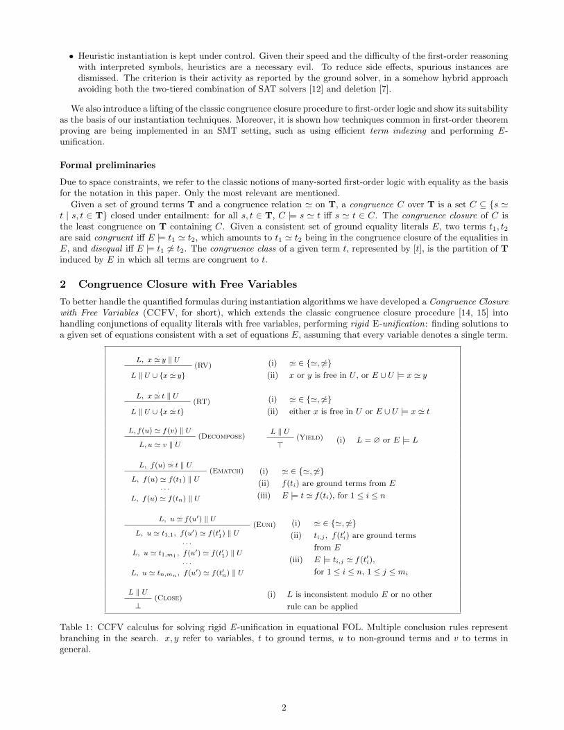
To better handle the quantified formulas during instantiation algorithms we have developed a Congruence Closurewith Free Variables (CCFV, for short), which extends the classic congruence closure procedure [14, 15] intohandling conjunctions of equality literals with free variables, performing rigid E-unification: finding solutions toa given set of equations consistent with a set of equations E, assuming that every variable denotes a single term.

L, x ' y ‖ U(RV)

L ‖ U ∪ {x ' y}(i) ' ∈ {', 6'}(ii) x or y is free in U , or E ∪ U |= x ' y

L, x ' t ‖ U(RT)

L ‖ U ∪ {x ' t}(i) ' ∈ {', 6'}(ii) either x is free in U or E ∪ U |= x ' t

L, f(u) ' f(v) ‖ U(Decompose)

L, u ' v ‖ U

L ‖ U(Yield)

>(i) L = ∅ or E |= L

L, f(u) ' t ‖ U(Ematch)

L, f(u) ' f(tn) ‖ U. . .

L, f(u) ' f(t1) ‖ U(i) ' ∈ {', 6'}(ii) f(ti) are ground terms from E

(iii) E |= t ' f(ti), for 1 ≤ i ≤ n

L, u ' f(u′) ‖ U(Euni)

L, u ' tn,mn , f(u′) ' f(t′n) ‖ U. . .

L, u ' t1,m1 , f(u′) ' f(t′1) ‖ U. . .

L, u ' t1,1, f(u′) ' f(t′1) ‖ U(i) ' ∈ {', 6'}(ii) ti,j , f(t′i) are ground terms

from E

(iii) E |= ti,j ' f(t′i),

for 1 ≤ i ≤ n, 1 ≤ j ≤ mi

L ‖ U(Close)

⊥(i) L is inconsistent modulo E or no other

rule can be applied

Table 1: CCFV calculus for solving rigid E -unification in equational FOL. Multiple conclusion rules representbranching in the search. x, y refer to variables, t to ground terms, u to non-ground terms and v to terms ingeneral.

2

Our procedure implements the rules1 shown in Table 1. To simplify presentation, it is assumed, without lossof generality, that function symbols are unary. Rules are shown only for equality literals, as their extensioninto uninterpreted predicates is straightforward. The calculus operates on conjunctive sets of equality literalscontaining free variables, annotated with equality literals between these variables and ground terms or themselves.Initially the annotations are empty, being augmented as the rules are applied and the input problem is simplified,embodying its solution.

CCFV algorithm

Given a set of ground equality literals E and a set of non ground equality literals L whose free variables are X,CCFV computes sets of equality literals U1, . . . , Un, denoted unifiers. Each unifier associates variables from Xto ground terms and allows the derivation of ground substitutions σ1, . . . , σk such that E |= Lσi, if any:

σi =

{x 7→ t x ∈ X; U |= x ' t for some ground term t. If x is free

in U , t is a ground term selected from its sort class.

}Since not necessarily all variables in X are congruent to ground terms in a given unifier U (denoted “free in U”),more than one ground substitution may be obtained by assigning those variables to different ground terms intheir sort classes.

A terminating strategy for CCFV is to apply the rules of Table 1 exhaustively over L, except that Ematch

may not be applied over the literals it introduces. There must be a backtracking when a given branch results inClose, until being able to apply Yield. In those cases a unifier is provided from which substitutions solving thegiven E -unification problem can be extracted.

Term Indexing

Performing E -unification requires dealing with many terms, which makes the use of an efficient indexing techniquefor fast retrieval of candidates paramount.

The Congruence Closure procedure in veriT keeps a signature table, in which terms and predicate atoms arekept modulo their congruence classes. For instance, if a ' b and both f(a) and f(b) appear in the formula,only f(a) is kept in the signature table. Those are referred to as signatures and are the only relevant terms forindexing, since instantiations into terms with the same signature are logically equivalent modulo the equalitiesin the current context. The signature table is indexed by top symbol2, such that each function and predicatesymbol points to all their related signatures. Those are kept sorted by congruence classes, to be amenable forbinary search. Bitmasks are kept to fast check whether a class contains signatures with a given top symbol, anecessary condition for retrieving candidates from that class.

A side effect of building the term index from the signature table is that all terms are considered, regardless ofwhether they appear or not in the current SAT solver model. To tackle this issue, an alternative index is builtdirectly from the currently asserted literals while computing on the fly the respective signatures. Dealing directlywith the model also has the advantage of allowing its minimization, since the SAT solver generally asserts moreliterals than necessary. Computing a prime implicant, a minimal partial model, can be done in linear time [9].Moreover, the CNF overhead is also cleaned: removing literals introduced by the non-equivalency preservingCNF transformation the formula undergoes, applying the same process described in [7] for Relevancy.

Implementing E-unification

The main data structure for CCFV is the “unifiers”: for a set of variables X, an array with each positionrepresenting a valuation for a variable x ∈ X, which consists of:

• a field for the respective variable;

• a flag to whether that variable is the representative of its congruence class;

• a field for, if the variable is a representative, the ground term it is equal to and a set of terms it is disequalto; otherwise a pointer to the variable it is equal to, the default being itself.

1The calculus still needs to be improved, with a better presentation and the proofs of its properties, which are work in progress.2Since top symbol indexing is not optimal, the next step is to implement fingerprint indexing. The current implementation keeps

the indexing as modular as possible to facilitate eventually changing its structure.

3

Each unifier represents one of the sets U mentioned above. They are handled with a UNION-FIND algorithmwith path-compression. The union operation is made modulo the congruence closure on the ground terms andthe current assignments to the variables in that unifier, which maintains the invariant of it being a consistentset of equality literals.

The rules in Table 1 are implemented as an adaptation of the recursive descent E-unification algorithm in [1],heavily depending on the term index described shown above for optimizing the search. Currently it does nothave a dedicated index for performing unification, rather relying in the DAG structure of the terms. To avoid(usually expensive) re-computations, memoization is used to store the results of E -unifications attempts, whichis particularly useful when looking for unifiers for, e.g., f(x) ' g(y) in which both “f ” and “g” have large termindexes. For now these “unification jobs” are indexed by the literal’s polarity and participating terms, not takinginto account their structure.

3 Instantiation Framework

3.1 Goal-oriented instantiation

In the classic architecture of SMT solving, a SAT solver enumerates boolean satisfiable conjunctions of literalsto be checked for ground satisfiability by decision procedures for a given set of theories. If these models are notrefuted at the ground level they must be evaluated at the first-order level, which is not a decidable problem ingeneral. Therefore one cannot assume to have an efficient algorithm to analyze the whole model and determineif it can be refuted. This led to the regular heuristic instantiation in SMT solving being not goal-oriented: itssearch is based solely on pattern matching of selected triggers [10], without further semantic criteria, which canbe performed quickly and then revert the reasoning back to the efficient ground solver.

In [19], Reynolds et al. presented an efficient incomplete goal-oriented instantiation technique that evaluatesa quantified formula, independently, in search for conflicting instances: given a satisfiable conjunctive set ofground literals E, a set of quantified formulas Q and some ∀x.ψ ∈ Q it searches for a ground substitution σ suchthat E |= ¬ψσ. Such substitutions are denoted ground conflicting, with conflicting instances being such that∀x.ψ → ψσ refutes E ∪Q.

Since the existence of such substitutions is an NP-complete problem equivalent to Non-simultaneous rigidE-unification [20], the CCFV procedure is perfectly suited to solve it. Each quantified formula ∀x.ψ ∈ Q isconverted into CNF and CCFV is applied for computing sequences of substitutions3 σ0, . . . , σk such that, for¬ψ = l1 ∧ · · · ∧ lk,

σ0 = ∅; σi−1 ⊆ σi and E |= liσi

which guarantees that E |= ¬ψσk and that the instantiation lemma ∀x.ψ → ψσk refutes E ∪Q. If any literalli+i is not unifiable according to the unifications up to li, there are no conflicting instances for ∀x.ψ.

Currently our implementation applies a breadth-first search on the conjunction of non-ground literals, com-puting all unifiers for a given literal l ∈ ¬ψ before considering the next one. Memory consumption is an issuedue to the combinatorial explosion that might occur when merging sets of unifiers from different literals. Amore general issue is simply the time required for finding the unifiers of a given literal, which can have a hugesearch space depending on the number of indexed terms. To minimize these problems customizable parametersset thresholds both on the number of potential combinations and of terms to be considered.

3.2 Heuristic instantiation with instances dismissal

Although goal-oriented search avoids heuristic instantiation in many cases, triggers and pattern-matching are stillthe backbone of our framework. A well known side effect of them is the production of many spurious instanceswhich not only interfere with the performances of both the ground and instantiation modules but also may leadto matching loops: triggers generating instances which are used solely to produce new instances in an infinitechain. To avoid this issues, de Moura et al. [7] mention how they perform clause deletion, during backtracking,of instances which were not part of a conflict. However, this proved to be an engineering challenge in veriT, sinceits original architecture does not easily allow deletion of terms from the ground solver.

3Since CCFV is non-proof confluent calculus, as choices may need to be made whenever a matching or unification must beperformed, backtracks are usually necessary for exploring different options.

4

To circumvent this problem, instead of being truly deleted instances are simply dismissed : by labeling themwith instantiation levels4, at a given level n only instances whose level is at most n− 1 are considered. This isdone by using the term indexing from the SAT model and eliminating literals whose instantiation level is abovethe threshold. At each instantiation round, the level is defined as the current level plus one. At the beginningof the solving all clauses are assigned level 0, the starting value for the instantiation level. At the end of aninstantiation round, the SAT solver is notified that at that point in the decision tree there was an instantiation,so that whenever there is a backtracking to a point before such a mark the instantiation level is decremented, atthe same time that all instances which have participated in a conflict are promoted to “level 0”. This ensuresthat those instances will not be dismissed for instantiation, which somehow emulates clause deletion. With thistechnique, however, the ground solver will still be burdened by the spurious instances, but they also will notneed to be regenerated in future instantiation rounds.

. . .

I1′

. . .

. . .

I2′

⊥3

I2

⊥2

I1

⊥1

. . .

⊥

Figure 1: Example of instance dismissal

Consider in Figure 1 an example of instance dismissal. I1 marks an instantiation happening at level 1, in whichall clauses from the original formula are considered for instantiation. Those lead to a conflict and a backtrackto a point before I1, which decrements the instantiation level to 0. All instances from I1 which were part of theconflict in ⊥1 are promoted to level 0, the rest kept with level 1. At I1′ only terms in clauses with level 0 areindexed. Since subsequently there is no backtracking to a point before I1′ , the instantiation level is increased to1. At I2 all clauses of level 1 are considered, thus including those produced both in I1 and I1′ . After a backtrack,the level is decremented to 1 and the instances participating in ⊥2 are promoted. This way at I2′ only thepromoted instances from the previous round are considered. Then the ground solver reaches a conflict in ⊥3 andcannot produce any more models, concluding unsatisfiability.

4 Experiments

The above techniques have been implemented in the SMT solver veriT [6], which previously offered support forquantified formulas solely through naıve trigger instantiation, without further optimizations5. The evaluationwas made on the “UF”, “UFLIA”, “UFLRA” and “UFIDL” categories of SMT-LIB [5], which have 10, 495benchmarks annotated as unsatisfiable. They consist mostly of quantified formulas over uninterpreted functionsas well as equality and linear arithmetic. The categories with bit vectors and non-linear arithmetic are currentlynot supported by veriT and in those in which uninterpreted functions are not predominant the techniques shownhere are not quite as effective yet. Our experiments were conducted using machines with 2 CPUs Intel XeonE5-2630 v3, 8 cores/CPU, 126GB RAM, 2x558GB HDD. The timeout is set for 30 seconds, since our goal isevaluating SMT solvers as backends of verification and ITP platforms, which require fast answers.

The different configurations of veriT are identified in this section according to which techniques they haveactivated:

• veriT: the solver relying solely on naıve trigger instantiation;

• veriT i: the solver with CCFV and the signature table indexed;

• veriT ig: besides the above, uses the goal-oriented search for conflicting instances;

4This is done much in the spirit of [11], although their labeling does not take into account the interactions with the SAT solverand is aimed at preventing matching loops, not towards “deletion”.

5A development version is available at http://www.loria.fr/~hbarbosa/veriT-ccfv.tar.gz

5

• veriT igd: does the term indexing from the SAT solver and uses the goal-oriented search and instancedismissal.

Figure 2a shows the big impact of the handling of instantiation by CCFV: veriT i is significantly faster andsolves 326 problems exclusively, while the old configuration solves only 32 exclusively. Figure 2b presents asignificant improvement in terms of problems solved (474 more against 36 less) by the use of the goal-orientedinstantiation, but it also shows a less clear gain of time. Besides the natural chaotic behavior of trigger instan-tiation, we believe this is due to the more expensive search performed: trying to falsify quantified formulas andhandling E -unification, which, in the context of SMT, has a much bigger search space than simply performingE -matching for pattern-matching instantiation. Not always the “better quality” of the conflicting instances off-sets the time it took to compute them, which indicates the necessity of trying to identify beforehand such casesand avoid the more expensive search when counter-producent.

0.1

1

10

0.1 1 10

veriT

_i

veriT

0.1

1

10

0.1 1 10

veriT

_i

veriT

0.1

1

10

0.1 1 10

veriT

_i

veriT

0.1

1

10

0.1 1 10

veriT

_i

veriT

(a) Impact of CCFV, without goal-oriented instantiation

0.1

1

10

0.1 1 10ve

riT_ig

veriT_i

0.1

1

10

0.1 1 10ve

riT_ig

veriT_i

0.1

1

10

0.1 1 10ve

riT_ig

veriT_i

0.1

1

10

0.1 1 10ve

riT_ig

veriT_i

(b) Impact of goal-oriented instantiation

Figure 2: Comparisons of new term indexing, CCFV and goal-oriented search

Logic Class CVC4 Z3 veriT igd veriT ig veriT i veriT

UFgrasshopper 410 418 431 437 418 413sledgehammer 1412 1249 1293 1272 1134 1066

UFIDL all 61 62 56 58 58 58

UFLIA

boogie 841 852 722 681 660 661sexpr 15 26 15 7 5 5grasshopper 320 341 356 367 340 335sledgehammer 1892 1581 1781 1778 1620 1569simplify 770 831 797 803 735 690simplify2 2226 2337 2277 2298 2291 2177Total 7947 7697 7727 7701 7203 6916

Table 2: Comparison between instantiation based SMT solvers on SMT-LIB benchmarks

Our new implementations were also evaluated against the SMT solvers Z3 [8] (version 4.4.2) and CVC4 [3](version 1.5), both based on instantiation for handling quantified formulas. The results are summarized in Table 2,excluding categories whose problems are trivially solved by all systems, which leaves 8, 701 for consideration.

While veriT ig and veriT igd solve a similar number of problems in the same categories (with a small advantageto the latter), it should be noted that they have quite diverse results depending on the benchmark (a comparisonis shown in Figure 4 at Appendix A). Each configuration solves ≈ 150 problems exclusively. This indicates thepotential to use both the term indexes, from the signature table and from the SAT solver model with instancedismissal, during the solving.

Regarding overall performance, CVC4 solves the most problems, being the more robust SMT solver forinstantiation and also applying a goal-oriented search for conflicting instances. Both configurations of veriT solveapproximately the same number of problems as Z3, although mostly because of the better performance on the

6

sledgehammer benchmarks, which have less theory symbols. There are 124 problems solved by veriT igd thatneither CVC4 nor Z3 solve, while veriT ig solves 115 that neither of these two do.

Figure 3 shows how the better veriT configuration, with the goal-oriented search and instance dismissal,performs against the other solvers. There are many problems solved exclusively by each system, which indicatesthe benefit of combining veriT with those systems them in a portfolio when trying to quickly solve a particularproblem: while CVC4 alone solves ≈ 92% of the considered benchmarks in 30s, by giving each of the fourcompared systems 7s is enough to solve ≈ 97% of them.

0.1

1

10

0.1 1 10

z3

veriT_igd

0.1

1

10

0.1 1 10

z3

veriT_igd

0.1

1

10

0.1 1 10

z3

veriT_igd

0.1

1

10

0.1 1 10

z3

veriT_igd

(a) Z3 vs veriT igd

0.1

1

10

0.1 1 10

cvc4

veriT_igd

0.1

1

10

0.1 1 10

cvc4

veriT_igd

0.1

1

10

0.1 1 10

cvc4

veriT_igd

0.1

1

10

0.1 1 10

cvc4

veriT_igd

(b) CVC4 vs veriT igd

Figure 3: Comparisons with SMT solvers

5 Conclusion and future work

There is still room for improvement in our instantiation framework. Particularly, a better understanding of theinstance dismissal effects is still required. Further analyzing the clauses activity would lead to a more refinedpromotion strategy and possibly better outcomes. Nevertheless, we believe that our preliminary results arepromising.

Regarding the term indexing, besides improving the data structures our main goal is performing it incremen-tally : by indexing the literals from the SAT model it is not necessary to thoroughly recompute the index ateach instantiation round. It is sufficient to simply remove or add terms, as well as update signatures, accordingto how the model has changed. The same principle may be applied to the memoization of “unification jobs”:an incremental term index would allow updating the resulting unifiers accordingly, significantly reducing theinstantiation effort over rounds with similar indexes.

Our goal-oriented instantiation has a very limited scope: currently conflicting instances can only be foundwhen a single quantified formula is capable of refuting the model. As it has been shown in [19] and also in ourown experiments this is enough to provide large improvements over trigger instantiation, but for many problemsit is still insufficient. We intend to combine CCFV with the Connection Calculus [17], a complete goal-orientedproof procedure for first-order logic, in an effort for having a broader approach for deriving conflicting instances.This would present a much more complex search space than the one our strategy currently handles. Thereforethe trade-off between expressivity and cost has to be carefully evaluated.

Applying different strategies in a portfolio approach is highly beneficial for solving more problems, but it couldbe even more so if different configurations were to communicate. Attempting pseudo-concurrent architecturessuch as described in [18] in veriT is certainly worth considering.

Acknowledgments

I would like to thank my supervisors Pascal Fontaine and David Deharbe for all their help throughout thedevelopment of this work and comments on the article.

Experiments presented in this paper were carried out using the Grid’5000 testbed, supported by a scien-tific interest group hosted by Inria and including CNRS, RENATER and several Universities as well as otherorganizations (see https://www.grid5000.fr).

7

References

[1] F. Baader and W. Snyder. Unification theory. In Handbook of Automated Reasoning (in 2 volumes), pages445–532. 2001.

[2] L. Bachmair and H. Ganzinger. Rewrite-Based Equational Theorem Proving with Selection and Simplifica-tion. J. Log. Comput., 4(3):217–247, 1994.

[3] C. Barrett, C. L. Conway, M. Deters, L. Hadarean, D. Jovanovic, T. King, A. Reynolds, and C. Tinelli.CVC4. In G. Gopalakrishnan and S. Qadeer, editors, Computer Aided Verification: 23rd International Con-ference, CAV 2011, Snowbird, UT, USA, July 14-20, 2011. Proceedings, pages 171–177, Berlin, Heidelberg,2011. Springer Berlin Heidelberg.

[4] C. Barrett, R. Sebastiani, S. Seshia, and C. Tinelli. Satisfiability Modulo Theories. In A. Biere, M. J. H.Heule, H. van Maaren, and T. Walsh, editors, Handbook of Satisfiability, volume 185 of Frontiers in ArtificialIntelligence and Applications, chapter 26, pages 825–885. IOS Press, Feb. 2009.

[5] C. Barrett, A. Stump, and C. Tinelli. The SMT-LIB Standard: Version 2.0. In A. Gupta and D. Kroening,editors, Proceedings of the 8th International Workshop on Satisfiability Modulo Theories (Edinburgh, UK),2010.

[6] T. Bouton, D. C. B. de Oliveira, D. Deharbe, and P. Fontaine. veriT: An Open, Trustable and EfficientSMT-Solver. In Automated Deduction - CADE-22, 22nd International Conference on Automated Deduction,Montreal, Canada, August 2-7, 2009. Proceedings, pages 151–156, 2009.

[7] L. de Moura and N. Bjørner. Efficient E-Matching for SMT Solvers. In F. Pfenning, editor, AutomatedDeduction CADE-21, volume 4603 of Lecture Notes in Computer Science, pages 183–198. Springer BerlinHeidelberg, 2007.

[8] L. M. de Moura and N. Bjørner. Z3: An Efficient SMT Solver. In Tools and Algorithms for the Constructionand Analysis of Systems, 14th International Conference, TACAS 2008, Held as Part of the Joint EuropeanConferences on Theory and Practice of Software, ETAPS 2008, Budapest, Hungary, March 29-April 6, 2008.Proceedings, pages 337–340, 2008.

[9] D. Deharbe, P. Fontaine, D. Le Berre, and B. Mazure. Computing Prime Implicants. In FMCAD - FormalMethods in Computer-Aided Design 2013, pages 46–52, Portland, United States, Oct. 2013. IEEE.

[10] D. Detlefs, G. Nelson, and J. B. Saxe. Simplify: A Theorem Prover for Program Checking. J. ACM,52(3):365–473, May 2005.

[11] Y. Ge, C. Barrett, and C. Tinelli. Solving Quantified Verification Conditions Using Satisfiability Mod-ulo Theories. In F. Pfenning, editor, Automated Deduction CADE-21, volume 4603 of Lecture Notes inComputer Science, pages 167–182. Springer Berlin Heidelberg, 2007.

[12] K. R. M. Leino, M. Musuvathi, and X. Ou. A Two-tier Technique for Supporting Quantifiers in a LazilyProof-explicating Theorem Prover. In Proceedings of the 11th International Conference on Tools and Algo-rithms for the Construction and Analysis of Systems, TACAS’05, pages 334–348, Berlin, Heidelberg, 2005.Springer-Verlag.

[13] L. Moura and N. Bjørner. Engineering DPLL(T) + Saturation. In Proceedings of the 4th International JointConference on Automated Reasoning, IJCAR ’08, pages 475–490, Berlin, Heidelberg, 2008. Springer-Verlag.

[14] G. Nelson and D. C. Oppen. Fast Decision Procedures Based on Congruence Closure. J. ACM, 27(2):356–364, Apr. 1980.

[15] R. Nieuwenhuis and A. Oliveras. Fast congruence closure and extensions. Information and Computation,205(4):557 – 580, 2007. Special Issue: 16th International Conference on Rewriting Techniques and Applica-tions.

[16] R. Nieuwenhuis and A. Rubio. Paramodulation-Based Theorem Proving. In A. Robinson and A. Voronkov,editors, Handbook of automated reasoning, volume 1, pages 371–443. 2001.

8

[17] J. Otten. Restricting backtracking in connection calculi. AI Commun., 23(2-3):159–182, 2010.

[18] G. Reger, D. Tishkovsky, and A. Voronkov. Cooperating Proof Attempts. In Automated Deduction -CADE-25 - 25th International Conference on Automated Deduction, Berlin, Germany, August 1-7, 2015,Proceedings, pages 339–355, 2015.

[19] A. Reynolds, C. Tinelli, and L. de Moura. Finding Conflicting Instances of Quantified Formulas in SMT.In Proceedings of the 14th Conference on Formal Methods in Computer-Aided Design, FMCAD ’14, pages31:195–31:202, Austin, TX, 2014. FMCAD Inc.

[20] A. Tiwari, L. Bachmair, and H. Ruess. Rigid E-Unification Revisited. In D. McAllester, editor, AutomatedDeduction - CADE-17, volume 1831 of Lecture Notes in Computer Science, pages 220–234. Springer BerlinHeidelberg, 2000.

9

Appendix A

0.1

1

10

0.1 1 10

veriT

_ig

d

veriT_ig

0.1

1

10

0.1 1 10

veriT

_ig

d

veriT_ig

0.1

1

10

0.1 1 10

veriT

_ig

d

veriT_ig

0.1

1

10

0.1 1 10

veriT

_ig

d

veriT_ig

Figure 4: Comparison of the two strategies

10

Handling Common Transitive Relations

in First-Order Automated Reasoning

Koen Claessen Ann Lilliestrom

Chalmers University of Technology{koen,annl}@chalmers.se

Abstract

We present a number of alternative ways of handling transitive binaryrelations that commonly occur in first-order problems, in particularequivalence relations, total orders, and reflexive, transitive relations.We show how such relations can be discovered syntactically in an in-put theory. We experimentally evaluate different treatments on prob-lems from the TPTP, using resolution-based reasoning tools as well asinstance-based tools. Our conclusions are that (1) it is beneficial toconsider different treatments of binary relations as a user, and that (2)reasoning tools could benefit from using a preprocessor or even built-insupport for certain binary relations.

1 Introduction

Most automated reasoning tools for first-order logic have some kind of built-in support for reasoning about equal-ity. Equality is one of the most common binary relations, and there are great performance benefits from providingbuilt-in support for equality. Together, these two advantages by far outweigh the cost of implementation.

Other common concepts for which there exists built-in support in many tools are associative, commutativeoperators; and real-valued, rational-valued, and integer-valued arithmetic. Again, these concepts seem to appearoften enough to warrant the extra cost of implementing special support in reasoning tools.

This paper is concerned with investigating what kind of special treatment we could give to commonly appearingtransitive binary relations, and what effect this treatment has in practice. Adding special treatment of transitiverelations to reasoning tools has been the subject of study before, in particular by means of chaining [1]. Thetransitivity axiom

@x , y , z . Rpx , yq ^ Rpy , z q ñ Rpx , z q

can lead to an expensive proof exploration in resolution and superposition based theorem provers, and cangenerate a huge number of instances in instance-based provers and SMT-solvers. Transitive relations are alsocommon enough to motivate special built-in support. However, as far as we know, chaining is not implementedin any of the major first-order reasoning tools (at least not in E [6], Vampire [5], Z3 [4], and CVC4 [2], whichwere used in this paper).

As an alternative to adding built-in support, in this paper we mainly look at (1) what a user of a reasoningtool may do herself to optimize the handling of these relations, and (2) how a preprocessing tool may be able todo this automatically. Adding built-in reasoning support in the tools themselves is not a main concern of thispaper.

Copyright c© by the paper’s authors. Copying permitted for private and academic purposes.

In: P. Fontaine, S. Schulz, J. Urban (eds.): Proceedings of the 5th Workshop on Practical Aspects of Automated Reasoning(PAAR 2016), Coimbra, Portugal, 02-07-2016, published at http://ceur-ws.org

11

reflexive ” @x . Rpx , x qeuclidean ” @x , y , z . Rpx , yq ^ Rpx , z q ñ Rpy , z qantisymmetric ” @x , y . Rpx , yq ^ Rpy , x q ñ x “ ytransitive ” @x , y , z . Rpx , yq ^ Rpy , z q ñ Rpx , z qasymmetric ” @x , y . Rpx , yq _ Rpy , x qtotal ” @x , y . Rpx , yq _ Rpy , x qsymmetric ” @x , y . Rpx , yq ñ Rpy , x qcoreflexive ” @x , y . Rpx , yq ñ x “ y

Figure 1: Definitions of basic properties of binary relations

By “treatment” we mean any way of logically expressing the relation. For example, a possible treatment of abinary relation R in a theory T may simply mean axiomatizing R in T . But it may also mean transforming Tinto a satisfiability-equivalent theory T 1 where R does not even syntactically appear.

As an example, consider a theory T in which an equivalence relation R occurs. One way to deal with R is tosimply axiomatize it, by means of reflexivity, symmetry, and transitivity:

@x . Rpx , x q@x , y . Rpx , yq ñ Rpy , x q@x , y , z . Rpx , yq ^ Rpy , z q ñ Rpx , z q

Another way is to “borrow” the built-in equality treatment that exists in most theorem provers. We can do thisby introducing a new symbol rep, and replacing all occurrences of Rpx , yq by the formula:

reppx q “ reppyq

The intuition here is that rep is now the representative function of the relation R. No axioms are needed. Aswe shall see, this alternative treatment of equivalence relations is satisfiability-equivalent with the original one,and actually is beneficial in practice in certain cases.

In general, when considering alternative treatments, we strive to make use of concepts already built-in to thereasoning tool in order to express other concepts that are not built-in.

For the purpose of this paper, we have decided to focus on three different kinds of transitive relations: (1)equivalence relations and partial equivalence relations, (2) total orders and strict total orders, and (3) generalreflexive, transitive relations. The reason we decided to concentrate on these three are because (a) they appearfrequently in practice, and (b) we found well-known ways but also novel ways of dealing with these.

The target audience for this paper is thus both people who use reasoning tools and people who implementreasoning tools.

2 Common properties of binary relations

In this section, we take a look at commonly occurring properties of binary relations, which combinations of theseare interesting for us to treat specially, and how we may go about discovering these.

Take a look at Fig. 1. It lists 8 basic and common properties of binary relations. Each of these properties canbe expressed using one logic clause, which makes it easy to syntactically identify the presence of such a propertyin a given theory.

When we investigated the number of occurrences of these properties in a subset of the TPTP problem library1

[7], we ended up with the table in Fig. 2. The table was constructed by gathering all clauses from all TPTPproblems (after clausification), and keeping every clause that only contained one binary relation symbol and,possibly, equality. Each such clause was then categorized as an expression of a basic property of a binary relationsymbol. We found only 163 such clauses that did not fit any of the 8 properties we chose as basic properties,but were instead instances of two new properties. Both of these were quite esoteric and did not seem to have astandard name in mathematics.

The table also contains occurrences where a negated relation was stated to have a certain property, and alsooccurrences where a flipped relation (a relation with its arguments swapped) was stated to have a certain property,

1For the statistics in this paper, we decided to only look at unsorted TPTP problems with 10.000 clauses or less.

12

4945 reflexive2082 euclidean1874 antisymmetric1567 transitive784 asymmetric784 total388 symmetric

3 coreflexive(163 other)

Figure 2: Number of occurrences of binary relation properties in TPTP

430+18 equivalence relations181+7 partial equivalence relations328+7 (strict) total orders

573+20 reflexive, transitive relations (excluding the above)

Figure 3: Number of occurrences of binary relations in TPTP, divided up into Theo-rem/Unsatisfiable/Unknown/Open problems + Satisfiable/CounterSatisfiable problems.

and also occurrences of combined negated and flipped relations. This explains for example why the number ofoccurrences of total relations is the same as for asymmetric relations; if a relation is total, the negated relationis asymmetric and vice-versa.

We adopt the following notation. Given a property of binary relations prop, we introduce its negated version,which is denoted by prop . The property prop holds for R if and only if prop holds for R. Similarly, weintroduce the flipped version of a property prop, which is denoted by propò. The property propò holds for R ifand only if prop holds for the flipped version of R.

Using this notation, we can for example say that total is equivalent with asymmetric . Sometimes theproperty we call euclidean here is called right euclidean; the corresponding variant left euclidean can be denotedeuclideanò. Note that prop is not the same as prop! For example, a relation R can be reflexive, or reflexive

(which means that R is reflexive), or reflexive, which means that R is not reflexive.

Using this notation on the 8 original basic properties from Fig. 1, we end up with 32 new basic propertiesthat we can use. (However, as we have already seen, some of these are equivalent to others.)

This paper will look at 5 kinds of different binary relations, which are defined as combinations of basicproperties:

equivalence relation ” treflexive, symmetric, transitive upartial equivalence relation ” tsymmetric, transitive utotal order ” ttotal , antisymmetric, transitive ustrict total order ” tantisymmetric , asymmetric, transitive ureflexive, transitive relation ” treflexive, transitive u

As a side note, in mathematics, strict total orders are sometimes defined using a property called trichotomous,which means that exactly one of Rpx , yq, x “ y , or Rpy , x qmust be true. However, when you clausify this propertyin the presence of transitivity, you end up with antisymmetric which says that at least one of Rpx , yq, x “ y ,or Rpy , x q must be true. There seems to be no standard name in mathematics for the property antisymmetric ,which is why we use this name.

In Fig. 3, we display the number of binary relations we have found in (our subset of) the TPTP for eachcategory. The next section describes how we found these.

3 Syntactic discovery of common binary relations

If our goal is to automatically choose the right treatment of equivalence relations, total orders, etc., we musthave an automatic way of identifying them in a given theory. It is easy to discover for example an equivalencerelation in a theory by means of syntactic inspection. If we find the presence of the axioms reflexive, symmetric,and transitive, for the same relational symbol R, we know that R is an equivalence relation.

13

total ô totalò

total ô asymmetric

total ô asymmetric ò

reflexive ô reflexiveò

reflexive ô reflexive ò

symmetric ô symmetric

symmetric ô symmetricò

symmetric ô symmetric ò

transitive ô transitiveò

transitive ô transitive ò

coreflexive ô coreflexiveò

coreflexive ô coreflexive ò

antisymmetric ô antisymmetricò

antisymmetric ô antisymmetric ò

Figure 4: Basic properties that are equivalent

But there is a problem. There are other ways of axiomatizing equivalence relations. For example, a muchmore common way to axiomatize equivalence relations in the TPTP is to state the two properties reflexive andeuclidean for R.

Rather than enumerating all possible ways to axiomatize certain relations by hand, we wrote a program thatcomputes all possible ways for any combination of basic properties to imply any other combination of basicproperties. Our program generates a table that can be precomputed in a minute or so and then used to veryquickly detect any alternative axiomatization of binary relations using basic properties.

Let us explain how this table was generated. We start with a list of 32 basic properties (the 8 original basicproperties, plus their negated, flipped, and negated flipped versions). Firstly, we use an automated theoremprover (we used E [6]) to discover which of these are equivalent with other such properties. The result isdisplayed in Fig. 4. Thus, 17 basic properties can be removed from the list, because they can be expressed usingother properties. The list of basic properties now has 15 elements left.

Secondly, we want to generate all implications of the form tprop1, . . , propn u ñ prop where the settprop1, . . , propn u is minimal. We do this separately for each prop. The results are displayed in Fig. 5.

The procedure uses a simple constraint solver (a SAT-solver) to keep track of all implications it has tried sofar, and consists of one main loop. At every loop iteration, the constraint solver guesses a set tprop1, . . , propn u

from the set of all properties P´ tprop u. The procedure then asks E whether or not tprop1, . . , propn u ñ propis valid. If it is, then we look at the proof that E produces, and print the implication tpropa, . . , propb u ñ prop,where tpropa, . . , propb u is the subset of properties that were used in the proof. We then also tell the constraintsolver never to guess a superset of tpropa, . . , propbu again. If the guessed implication can not be proven, we tellthe constraint solver to never guess a subset of tprop1, . . , propn u again. The procedure stops when no guessesthat satisfy all constraints can be made anymore.

After the loop terminates, we may need to clean up the implications somewhat because some implicationsmay subsume others.

In order to avoid generating inconsistent sets tprop1, . . , propn u (that would imply any other property), wealso add the artificial inconsistent property false to the set, and generate implications for this property first. Weexclude any found implication here from the implication sets of the real properties.

This procedure generates a complete list of minimal implications. It works well in practice, especially if allguesses are maximized according to their size. The vast majority of the time is spent on the implication proofs,and no significant time is spent in the SAT-solver.

To detect a binary relation R with certain properties in a given theory, we simply gather all basic propertiesabout R that occur in the theory, and then compute which other properties they imply, using the pre-generatedtable. In this way, we never have to do any theorem proving in order to detect a binary relation with certainproperties.

14

false ð treflexive, reflexive u transitive ð teuclidean, antisymmetricufalse ð treflexive, asymmetricu transitive ð teuclidean, euclidean ufalse ð ttotal, reflexive u transitive ð ttotal, euclideanò

u

false ð ttotal, asymmetricu transitive ð tasymmetric, euclideanòu

reflexive ð ttotal u transitive ð tsymmetric, euclideanòu

euclidean ð tsymmetric, asymmetricu transitive ð tasymmetric, euclidean òu

euclidean ð ttotal, symmetricu transitive ð tantisymmetric, euclidean òu

euclidean ð tantisymmetric, coreflexive u transitive ð teuclidean, reflexive ueuclidean ð ttransitive, euclidean u transitive ð teuclidean, euclidean ò

u

euclidean ð tantisymmetric, euclidean u transitive ð teuclidean, euclideanòu

euclidean ð treflexive, coreflexive u transitive ð tantisymmetric, euclideanòu

euclidean ð treflexive, euclidean u transitive ð teuclideanò, antisymmetric ueuclidean ð tcoreflexive u transitive ð teuclidean , euclideanò

u

euclidean ð ttotal, coreflexive u total ð treflexive, coreflexive ueuclidean ð treflexive , euclideanò

u total ð treflexive, euclidean òu

euclidean ð treflexive, euclidean òu total ð treflexive, euclidean u

euclidean ð tasymmetric, euclideanòu total ð treflexive, antisymmetric u

euclidean ð tsymmetric, antisymmetricu total ð treflexive, transitive ueuclidean ð ttransitive, reflexive , euclidean ò

u symmetric ð tcoreflexive ueuclidean ð ttotal, euclidean u symmetric ð teuclidean , reflexive ueuclidean ð ttransitive, coreflexive u symmetric ð teuclidean, reflexive ueuclidean ð tasymmetric, coreflexive u symmetric ð tcoreflexive ueuclidean ð tasymmetric, euclidean u symmetric ð ttotal, euclidean ueuclidean ð ttotal, euclidean ò

u symmetric ð ttotal, euclidean ueuclidean ð tantisymmetric, reflexive , euclidean ò

u symmetric ð teuclidean, asymmetricueuclidean ð tasymmetric, euclidean ò

u symmetric ð tasymmetric, euclidean ueuclidean ð tsymmetric, transitive u symmetric ð treflexive, euclidean ò

u

euclidean ð teuclidean , euclideanòu symmetric ð treflexive, euclideanò

u

euclidean ð tsymmetric, euclideanòu symmetric ð treflexive , euclideanò

u

euclidean ð treflexive, euclideanòu symmetric ð treflexive , euclidean ò

u

euclidean ð treflexive, symmetric, antisymmetric u symmetric ð ttotal, euclidean òu

euclidean ð treflexive, symmetric, transitive u symmetric ð tasymmetric, euclideanòu

euclidean ð ttotal, euclideanòu symmetric ð teuclidean , euclideanò

u

euclidean ð teuclideanò, coreflexive u symmetric ð ttotal, euclideanòu

antisymmetric ð tcoreflexive u symmetric ð teuclidean, euclidean òu

antisymmetric ð tasymmetricu symmetric ð teuclidean, euclideanòu

antisymmetric ð ttransitive, reflexive u symmetric ð teuclidean, reflexive uantisymmetric ð treflexive , euclideanò

u symmetric ð tasymmetric, euclidean òu

antisymmetric ð teuclidean, reflexive u symmetric ð teuclidean , euclidean òu

transitive ð tsymmetric, asymmetricu symmetric ð treflexive, euclidean utransitive ð ttotal, symmetricu coreflexive ð tsymmetric, asymmetricutransitive ð tantisymmetric, coreflexive u coreflexive ð tantisymmetric, coreflexive utransitive ð tcoreflexive u coreflexive ð ttransitive, euclidean , reflexive utransitive ð teuclidean, transitive u coreflexive ð tasymmetric, coreflexive utransitive ð tsymmetric, antisymmetricu coreflexive ð teuclidean, reflexive utransitive ð treflexive, euclidean u coreflexive ð treflexive, antisymmetric, euclidean utransitive ð teuclidean, reflexive u coreflexive ð tasymmetric, euclidean utransitive ð ttotal, euclidean u coreflexive ð teuclidean, asymmetricutransitive ð treflexive, coreflexive u coreflexive ð tsymmetric, antisymmetricutransitive ð tasymmetric, coreflexive u coreflexive ð ttotal, antisymmetric, euclidean utransitive ð tasymmetric, euclidean u coreflexive ð treflexive, antisymmetric, euclidean ò

u

transitive ð tasymmetric, transitive u coreflexive ð treflexive, antisymmetric, euclideanòu

transitive ð tantisymmetric, transitive u coreflexive ð tsymmetric, transitive, reflexive utransitive ð teuclideanò, euclidean ò

u coreflexive ð ttransitive, reflexive , coreflexive utransitive ð teuclidean, coreflexive u coreflexive ð tantisymmetric, euclidean , euclideanò

u

transitive ð ttotal, coreflexive u coreflexive ð ttotal, antisymmetric, euclideanòu

transitive ð teuclidean, asymmetricu coreflexive ð ttotal, euclidean, antisymmetricutransitive ð ttotal, euclidean u coreflexive ð ttotal, antisymmetric, euclidean ò

u

transitive ð treflexive, euclidean òu coreflexive ð tantisymmetric, reflexive , euclidean ò

u

transitive ð teuclideanò, transitive u coreflexive ð treflexive , euclideanòu

transitive ð teuclidean, symmetricu coreflexive ð tantisymmetric, euclidean , reflexive utransitive ð treflexive , euclideanò

u coreflexive ð tasymmetric, euclideanòu

transitive ð tantisymmetric, euclidean u coreflexive ð tasymmetric, euclidean òu

transitive ð ttotal, euclidean òu coreflexive ð tantisymmetric, euclidean , euclidean ò

u

transitive ð teuclidean, antisymmetric u coreflexive ð teuclidean, antisymmetric, euclidean òu

transitive ð treflexive, euclideanòu coreflexive ð teuclidean, antisymmetric, euclideanò

u

transitive ð treflexive, symmetric, antisymmetric u coreflexive ð teuclidean, reflexive, antisymmetricutransitive ð teuclideanò, coreflexive u coreflexive ð ttransitive, reflexive , euclidean ò

u

transitive ð treflexive, symmetric, transitive u

Figure 5: The complete list of implications between properties

15

4 Handling equivalence relations

Equalification As mentioned in the introduction, an alternative way of handling equivalence relations R isto create a new symbol rep and replace all occurrences of R with a formula involving rep:

R reflexiveR symmetric _R transitiveT r. . Rpx , yq . .s T r. . reppx q “ reppyq . .s

To explain the above notation: We have two theories, one on the left-hand side of the arrow, and one on theright-hand side of the arrow. The transformation transforms any theory that looks like the left-hand side intoa theory that looks like the right-hand side. We write T r. . e . .s for theories in which e occurs syntactically; inthe transformation, all occurrences of e should be replaced.

We call the above transformation equalification. This transformation may be beneficial because the reasoningnow involves built-in equality reasoning instead of reasoning about an unknown symbol using axioms.

The transformation is correct, meaning that it preserves (non-)satisfiability: (ñ) If we have a model of theLHS theory, then R must be interpreted as an equivalence relation. Let rep be the representative function of R,in other words we have Rpx , yq ô reppx q “ reppyq. Thus we also have a model of the RHS theory. (ð) If wehave a model of the RHS theory, let Rpx , yq :“ reppx q “ reppyq. It is clear that R is reflexive, symmetric, andtransitive, and therefore we have model of the LHS theory.

In the transformation, we also remove the axioms for reflexivity, symmetry, and transitivity, because theyare not needed anymore. But what if R is axiomatized as an equivalence relation using different axioms? Thenwe can remove any axiom about R that is implied by reflexivity, symmetry, and transitivity. Luckily we havealready computed a table of which properties imply which other ones (shown in Fig. 5).

Pequalification There are commonly occurring binary relations called partial equivalence relations that almostbehave as equivalence relations, but not quite. In particular, they do not have to obey the axiom of reflexivity.Can we do something for these too?

It turns out that a set with a partial equivalence relation R can be partitioned into two subsets: (1) one subseton which R is an actual equivalence relation, and (2) one subset of elements which are not related to anything,not even themselves.

Thus, an alternative way of handling partial equivalence relations R is to create two new symbols, rep and P ,and replace all occurrences of R with a formula involving rep and P:

R symmetricR transitive _T r. . Rpx , yq . .s T r. . pP px q ^ P pyq ^ reppx q “ reppyqq . .s

Here, P is the predicate that indicates the subset on which R behaves as an equivalence relation.We call this transformation pequalification. This transformation may be beneficial because the reasoning now

involves built-in equality reasoning instead of reasoning about an unknown symbol using axioms. However, thereis also a clear price to pay since the size of the problem grows considerably.

The transformation is correct, meaning that it preserves (non-)satisfiability: (ñ) If we have a model of theLHS theory, then R must be interpreted as a partial equivalence relation. Let P px q :“Rpx , x q, in other words Pis the subset on which R behaves like an equivalence relation. Let rep be a representative function of R on P , inother words we have pP px q ^ P pyqq ñ pRpx , yq ô reppx q “ reppyqq. By the definition of P we then also haveRpx , yq ô pP px q ^ P pyq ^ reppx q “ reppyqq. Thus we also have a model of the RHS theory. (ð) If we have amodel of the RHS theory, let Rpx , yq :“ P px q ^ P pyq ^ reppx q “ reppyq. This R is symmetric and transitive,and therefore we have model of the LHS theory.

5 Handling total orders

Ordification Many reasoning tools have built-in support for arithmetic, in particular they support an orderď on numbers. It turns out that we can “borrow” this operator when handling general total orders. Suppose wehave a total order:

16

R : AˆA Ñ Bool

We now introduce a new injective function:

rep : A Ñ R

We then replace all occurrences of R with a formula involving rep in the following way:

R totalR antisymmetric _ @x , y . reppx q “ reppyq ñ x “ yR transitiveT r. . Rpx , yq . .s T r. . reppx q ď reppyq . .s

(Here, ď is the order on reals.) We call this transformation ordification. This transformation may be beneficialbecause the reasoning now involves built-in arithmetic reasoning instead of reasoning about an unknown symbolusing axioms.

The above transformation is correct, meaning that it preserves (non-)satisfiability: (ñ) If we have a modelof the LHS theory, then without loss of generality (by Lowenheim-Skolem), we can assume that the domain iscountable. Also, R must be interpreted as a total order. We now construct rep recursively as a mapping fromthe model domain to R, such that we have Rpx , yq ô reppx q ď reppyq, in the following way. Let ta0, a1, a2, . .ube the domain of the model, and set reppa0q :“ 0. For any n ą 0, pick a value for reppanq that is consistent withthe total order R and all earlier domain elements ai, for 0 ď i ă n. This can always be done because there isalways extra room for a new, unique element between any two distinct values of R. Thus rep is injective and wealso have a model of the RHS theory. (ð) If we have a model of the RHS theory, let Rpx , yq :“ reppx q ď reppyq.It is clear that R is total and transitive, and also antisymmetric because rep is injective, and therefore we havemodel of the LHS theory.

Note on Q vs. R The proof would have worked for Q as well instead of R. The transformation can thereforebe used for any tool that supports Q or R or both, and should choose whichever comparison operator is cheapestif there is a choice. Using integer arithmetic would however not have been correct.

Note on strict total orders One may have expected to have a transformation specifically targeted to stricttotal orders, i.e. something like:

R antisymmetric

R asymmetric _ @x , y . reppx q “ reppyq ñ x “ yR transitiveT r. . Rpx , yq . .s T r. . reppx q ă reppyq . .s

However, the transformation for total orders already covers this case! Any strict total order R is also recognizedas a total order R, and ordification already transforms such theories in the correct way. The only difference isthat Rpx , yq is replaced with preppx q ď reppyqq instead of reppx q ă reppyq, which is satisfiability-equivalent.(There may be a practical performance difference, which is not something we have investigated.)

Maxification Some reasoning tools do not have orders on real arithmetic built-in, but they may have otherconcepts that are built-in that can be used to express total orders instead. One such concept is handling ofassociative, commutative (AC) operators.

For such a tool, one alternative way of handling total orders R is to create a new function symbol max andreplace all occurrences of R with a formula involving max:

R total max associativeR antisymmetric _ max commutativeR transitive @x , y . maxpx , yq “ x _ maxpx , yq “ yT r. . Rpx , yq . .s T r. .maxpx , yq “ y . .s

We call this transformation maxification. This transformation may be beneficial because the reasoning nowinvolves built-in equality reasoning with AC unification (and one extra axiom) instead of reasoning about anunknown relational symbol (using three axioms).

17

The above transformation is correct, meaning that it preserves (non-)satisfiability: (ñ) If we have a modelof the LHS theory, then R must be interpreted as a total order. Let max be the maximum function associatedwith this order. Clearly, it must be associative and commutative, and the third axiom also holds. Moreover, wehave Rpx , yq ô maxpx , yq “ y . Thus we also have a model of the RHS theory. (ð) If we have a model of theRHS theory, let Rpx , yq :“maxpx , yq “ y . Given the axioms in the RHS theory, R is total, antisymmetric, andtransitive, and therefore we have model of the LHS theory.

(It may be the case that maxification can also be used to express orders that are weaker than total orders.At the time of this writing, we have not figured out how to do this.)

6 Handling reflexive, transitive relations

Transification The last transformation we present is designed as an alternative treatment for any relationthat is reflexive and transitive. It does not make use of any built-in concept in the tool. Instead, it transformstheories with a transitivity axiom into theories without that transitivity axiom. Instead, transitivity is specializedat each positive occurrence of the relational symbol.

As such, an alternative way of handling reflexive, transitive relations R is to create a new symbol Q andreplace all positive occurrences of R with a formula involving Q; the negative occurrences are simply replacedby Q:

R reflexive Q reflexiveR transitive _T r. . Rpx , yq . . T r. . p@r . Qpr , x q ñ Qpr , yqq . .

Rpx , yq . .s Qpx , yq . .s

We call this transformation transification. This transformation may be beneficial because reasoning abouttransitivity in a naive way can be very expensive for theorem provers, because from transitivity there are manypossible conclusions to draw that trigger each other “recursively”. The transformation only works on problemswhere every occurrence of R is either positive or negative (and not both, such as under an equivalence operator).If this is not the case, the problem has to be translated into one where this is the case. This can for example bedone by means of clausification.

Note that the resulting theory does not blow-up; only clauses with a positive occurrence of R gets one extraliteral per occurrence.

We replace any positive occurrence of Rpx , yq with an implication that says “for any r , if you could reach xfrom r , now you can reach y too”. Thus, we have specialized the transitivity axiom for every positive occurrenceof R.

Note that in the RHS theory, Q does not have to be transitive! Nonetheless, the transformation is correct,meaning that it preserves (non-)satisfiability: (ñ) If we have a model of the LHS theory, then R is reflexiveand transitive. Now, set Q px , yq :“ R px , yq. Q is obviously reflexive. We have to show that R px , yq implies@r . Qpr , x q ñ Qpr , yq. This is indeed the case because R is transitive. Thus we also have a model of the RHStheory. (ð) If we have a model of the RHS theory, then Q is reflexive. Now, set Rpx , yq :“@r . Qpr , x q ñ Qpr , yq.R is reflexive (by reflexivity of implication) and transitive (by transitivity of implication). Finally, we have toshow that Qpx , yq implies Rpx , yq, which is the same as showing that @r . Qpr , x q ñ Qpr , yq implies Qpx , yq,which is true because Q is reflexive. Thus we also have a model of the RHS theory.

7 Experimental results

We evaluate the effects of the different axiomatizations using two different resolution based theorem provers, E1.9 [6] (with the xAuto and tAuto options) and Vampire 4.0 [5] (with the casc mode option), and two SMT-solvers, Z3 4.4.2 [4] and CVC4 1.4 [2]. The experiments were performed on a 2xQuad Core Intel Xeon E5620processor with 24 GB physical memory, running at 2.4 GHz. We use a time limit of 5 minutes on each problem.

We started from a set of 11674 test problems from the TPTP, listed as Unsatisfiable, Theorem, Unknown orOpen (leaving out the very large theories). For each problem, a new theory was generated for each applicabletransformation. For most problems, no relation matching any of the given criteria was detected, and thus no newtheories were produced for these problems. Evaluation of reasoning tools on Satisfiable and CounterSatisfiableproblems is left as future work.

The experimental results are summarized in Fig. 6.

18

E Vampire Z3 CVC4equalification (430) 422 +4 -33 428 +0 -2 362 +50 -3 370 +18 -39pequalification (181) 96 +0 -34 93 +4 -9 38 +9 -4 59 +1 -11transification (573) 324 +2 -26 308 +26 -11 234 +10 -46 255 +13 -42ordification (328) n/a 296 +16 -12 238 +51 -13 267 +13 -15maxification (328) 273 +1 -23 296 +2 -0 238 +1 -41 267 +4 -0

Figure 6: Table showing for each theorem prover the number of test problems solved before the transformation,how many new problems are solved after the transformation, and the number of problems that could be solvedbefore but not after the transformation. (Total number of applicable problems for each transformation inparentheses). A +value in boldface indicates that there were hard problems (Rating 1.0) solved with thatcombination of treatment and theorem prover. An underlined -value indicates that time slicing (running bothmethods in 50% of the time each) solves a strictly larger superset of problems with that combination of treatmentand theorem prover.

7.1 Equivalence relations

Equivalence relations were present in 430 of the test problems. The majority of these problems appear in theGEO and SYN categories. Interestingly, among these 430 problems, there are only 23 problems whose equivalencerelations are axiomatized with transitivity axioms. The remaining 407 problems axiomatize equivalence relationswith euclidean and reflexivity axioms, as discussed in section 3. The number of equivalence relations in eachproblem ranges from 1 to 40, where problems with many equivalence relations all come from the SYN category.There is no clear correspondence between the number of equivalence relations in a problem and the performanceof the prover prior to and after the transformation.

Equalification As can be seen in Fig. 6, equalification performs very well with Z3, and somewhat well withCVC4, while it worsens the results of the resolution based provers, which already performed well on the originalproblems. Using a time slicing strategy, which runs the prover on the original problem for half the time and onthe transformed problem for the second half, solves a strict superset of problems than the original for all of thetheorem provers used in the evaluation. Fig. 7 shows in more detail the effect on solving times for the differenttheorem provers.

Pequalification In 181 of the test problems, relations that are transitive and symmetric, but not reflexive,were found. The majority of these problems are in the CAT and FLD categories of TPTP. All of the testedtheorem provers perform worse on these problems compared to the problems with true equivalence relations.This is also the case after performing pequalification. Pequalification turns out to be particularly bad for E,which solves 34 fewer problems after the transformation. Pequalification makes Z3 perform only slightly betterand Vampire and CVC4 slightly worse.

Hard problems solved using Pequalification After Pequalification, one problem with rating 1.0 (FLD041-2) is solved by Vampire. Rating 1.0 means that no known current theorem prover solves the problem in reasonabletime.

7.2 Total orders

Total orders were found in 328 problems. The majority are in the SWV category, and the remaining in HWV,LDA and NUM. In 77 of the problems, the total order is positively axiomatized, and in the other 251 problemsit is negative (and thus axiomatized as a strict total order). There is never more than one order present in anyof the problems.

Ordification For each of the problems, we ran the theorem provers with built-in support for arithmetic onthe problems before and after applying ordification. Vampire was run on a version in TFF format [8], and Z3and CVC4 on a version in SMT format [3]. The original problems were also transformed into TFF and SMTin order to achieve a relevant comparison. Ordification performs well for Z3, while for Vampire and CVC4 it isgood for some problems and bad for some. Fig. 8 shows how solving times are affected, and the diagrams alsoshow great potential for time slicing, in particular for Vampire and Z3.

Hard problems solved using Ordification After Ordification, 15 problems, all from the SWV category, withrating 1.0 are solved. (SWV004-1, SWV035+1, SWV040+1, SWV044+1, SWV049+1, SWV079+1, SWV100+1,

19

0.01

0.1

1

10

100

0.01 0.1 1 10 100

equal

ifie

d-E

original-E

0.01

0.1

1

10

100

0.01 0.1 1 10 100

equal

ifie

d-v

ampir

e

original-vampire

0.01

0.1

1

10

100

0.01 0.1 1 10 100

equal

ifie

d-z

3

original-z3

0.01

0.1

1

10

100

0.01 0.1 1 10 100

equal

ifie

d-c

vc4

original-cvc4

Figure 7: The time taken to solve problems, with and without equalification, using E, Vampire, Z3 and CVC4

SWV101+1, SWV108+1, SWV110+1, SWV113+1, SWV118+1, SWV120+1, SWV124+1, SWV130+1) Vam-pire and Z3 each solve 14 hard problems and CVC4 solves 13 of them. One problem (SWV004-1) is evencategorized as Unknown, which means that no prover has ever solved it. After ordification, all three proverswere able to solve it in less than a second.

Maxification Maxification, our second possible treatment of total orders, turned out to be disadvantageousto E and Z3, while having a small positive effect on Vampire and CVC4 (see Fig. 6).

7.3 Transitive and Reflexive relations

573 test problems include relations that are transitive and reflexive, excluding equivalence relations and totalorders. In all of them, transitivity occurs syntactically as an axiom. The problems come from a variety ofcategories, but a vast majority are in SET, SEU and SWV. Only about half of the original problems were solvedby each theorem prover, which may indicate that transitivity axioms are difficult for current theorem proversto deal with. We evaluate the performance of the theorem provers before and after transification. Problemsthat include equivalence relations and total orders are excluded, as the corresponding methods equalificationand ordification give better results and should be preferred. Vampire benefits the most from transification, andsolves 32 new problems after the transformation, while 10 previously solvable problems become unsolvable withinthe time limit. For E, the effect of transification is almost exclusively negative. Vampire also has a significantlyworse performance than E overall on the original problems that include relations that are transitive and reflexive.Both Z3 and CVC4 perform worse after the transformation, but time slicing can be a good way to improve theresults.

Hard problems solved using Transification After transification, two new problems with rating 1.0 aresolved, both by Vampire (SEU322+2 and SEU372+2).

20

0.01

0.1

1

10

100

0.01 0.1 1 10 100

ord

ifie

d-v

amp

ire

original-vampire

0.001

0.01

0.1

1

10

100

0.001 0.01 0.1 1 10 100

ord

ifie

d-Z

3

original-Z3

0.001

0.01

0.1

1

10

100

0.001 0.01 0.1 1 10 100

ord

ifie

d-C

VC

4

original-CVC4

Figure 8: Effects of ordification, using Vampire, Z3 and CVC4

Equalification and Transification Since all equivalence relations are transitive and reflexive, the methodfor transification works also on equivalence relations. Comparing the two methods on the 430 problems withequivalence relations, we concluded that equalification and transification work equally bad for E, Vampire andCVC4. Both transification and equalification improve the results for Z3, but equalification does so significantly.

Ordification and Transification We compared ordification and transification on the 328 problems containingtotal orders. Transification seems to make these problems generally more difficult for theorem provers to solve,while ordification instead improved the results on many of the problems. Transification makes the theoremprover perform worse on these problems also for E, which cannot make use of ordification since it does notprovide support for arithmetic.

8 Discussion, Conclusions, and Future Work

We have presented 5 transformations that can be applied to theories with certain transitive relations: equalifica-tion, pequalification, transification, ordification, and maxification. We have also created a method for syntacticdiscovery of binary relations where these transformations are applicable.

For users of reasoning tools that create their own theories, it is clear that they should consider using one ofthe proposed alternative treatments when writing theories. For all of our methods, there are existing theories forwhich some provers performed better on these theories than others. In particular, there exist 18 TPTP problemsthat are now solvable that weren’t previously.

For implementers of reasoning tools, our conclusions are less clear. For some combinations of treatmentsand provers (such as transification for Vampire, and equalification for Z3), overall results are clearly better,and we would thus recommend these treatments as preprocessors for these provers. Some more combinationsof treatments and provers lend themselves to a time slicing strategy that can solve strictly more problems, andcould thusly be integrated in a natural way in provers that already have the time slicing machinery in place.

Related Work Chaining [1] is a family of methods that limit the use of transitivity-like axioms in proofsby only allowing certain chains of them to occur in proofs. The result is a complete proof system that avoidsthe derivation of unnecessary consequences of transitivity. However, chaining is not implemented in any of thereasoning tools we considered for this paper. In personal communication with some of the authors, chaining-liketechniques have not been deemed important enough to be considered for implementation, and their preliminaryexperimental results were mostly negative.

Future Work There is a lot of room for improvements and other future work. There are many other relationsthat are more or less common that could benefit from an alternative treatment like the transformations describedin this paper. In particular, maxification seems to be an idea that could be applied to binary relations that areweaker than total orders, which may make this treatment more effective. But there are also other, non-transitiverelations that are of interest.

Ordification uses total orders as the base-transformation, and treats strict total orders as negated total orders.We would like to investigate more in which cases it may be beneficial to treat strict total orders differently fromtotal orders, and when to use ă on R instead of ď.

We would also like to investigate the effect of our transformations on Satisfiable and CounterSatisfiable

21

0.01

0.1

1

10

100

0.01 0.1 1 10 100

tran

sifi

ed-e

original-e

0.01

0.1

1

10

100

0.01 0.1 1 10 100

tran

sifi

ed-v

ampir

e

original-vampire

0.01

0.1

1

10

100

0.01 0.1 1 10 100

tran

sifi

ed-z

3

original-z3

0.01

0.1

1

10

100

0.01 0.1 1 10 100

tran

sifi

ed-c

vc4

original-cvc4

Figure 9: Effects of transification, using E, Vampire, Z3 and CVC4

problems. What would be the effect on finite model finders? Some transformations change the number ofvariables per clause, which will influence the performance of finite model finders. What happens to saturation-based tools? Is it easier or harder to saturate a problem after transformation? Evaluating these questions ishard, because we did not find many satisfiable problems in the TPTP that contained relevant relations (see Fig.3). Instead, we considered using Unsatisfiable problems, and measuring the time it takes to show the absence ofmodels up to a certain size.

There are other kinds of relations than binary relations. For example, we can have an ternary relation thatbehaves as an equivalence relation in its 2nd and 3rd argument. An alternative treatment of this relation wouldbe to introduce a binary function symbol rep. We do not know whether or not this occurs often, and if it is agood idea to treat higher-arity relational symbols specially in this way.

Lastly, we would like to look at how these ideas could be used inside a theorem prover; as soon as the proverdiscovers that a relation is an equivalence relation or a total order, one of our transformations could be applied,on the fly. The details of how to do this remain to be investigated.

References

[1] Leo Bachmair and Harald Ganzinger. Ordered chaining calculi for first-order theories of transitive relations.Journal of the ACM (JACM), 45(6):1007–1049, 1998.

[2] Clark Barrett, Christopher L. Conway, Morgan Deters, Liana Hadarean, Dejan Jovanovic, Tim King, AndrewReynolds, and Cesare Tinelli. CVC4. In Proceedings of the 23rd International Conference on Computer AidedVerification, CAV’11, pages 171–177, Berlin, Heidelberg, 2011. Springer-Verlag.

[3] Clark Barrett, Aaron Stump, Cesare Tinelli, Sascha Boehme, David Cok, David Deharbe, Bruno Dutertre,Pascal Fontaine, Vijay Ganesh, Alberto Griggio, Jim Grundy, Paul Jackson, Albert Oliveras, Sava Krsti,

22

Michal Moskal, Leonardo De Moura, Roberto Sebastiani, To David Cok, and Jochen Hoenicke. C.: TheSMT-LIB Standard: Version 2.0. Technical report, 2010.

[4] Leonardo de Moura and Nikolaj Bjørner. Z3: An Efficient SMT Solver. In Tools and Algorithms for theConstruction and Analysis of Systems, 14th International Conference, TACAS 2008, Held as Part of theJoint European Conferences on Theory and Practice of Software, ETAPS 2008, Budapest, Hungary, March29-April 6, 2008. Proceedings, volume 4963 of Lecture Notes in Computer Science, pages 337–340. Springer,2008.

[5] Laura Kovacs and Andrei Voronkov. First-Order Theorem Proving and Vampire. In Computer Aided Verifi-cation - 25th International Conference, CAV 2013, Saint Petersburg, Russia, July 13-19, 2013. Proceedings,pages 1–35, 2013.

[6] Stephan Schulz. The E Theorem Prover, 2015. http://www.eprover.org/.

[7] Geoff Sutcliffe. The TPTP Problem Library, 2015. http://www.tptp.org/.

[8] Geoff Sutcliffe, Stephan Schulz, Koen Claessen, and Peter Baumgartner. The TPTP Typed First-order Formand Arithmetic. In Nikolaj Bjørner and Andrei Voronkov, editor, The 18th International Conference on Logicfor Programming Artificial Intelligence and Reasoning (LPAR-18), pages 406–419, Merida, Venezuela, mar2012. Springer Verlag.

23

No Choice: Reconstruction of First-order ATP Proofswithout Skolem Functions

Michael Färbermichael.faerber@uibk.ac.at

Cezary Kaliszykcezary.kaliszyk@uibk.ac.at

Universität InnsbruckInnsbruck, Austria

Abstract

Proof assistants based on higher-order logic frequently use first-orderautomated theorem provers as proof search mechanisms. The recon-struction of the proofs generated by common tools, such as MESON andMetis, typically involves the use of the axiom of choice to simulate theSkolemisation steps. In this paper we present a method to reconstructthe proofs without introducing Skolem functions. This enables us tointegrate tactics that use first-order automated theorem provers in logicsthat feature neither the axiom of choice nor the definite descriptionoperator.

1 IntroductionMany first-order automated theorem provers (ATPs) operate on formulae with implicitly universally quantifiedvariables. To find proofs with such ATPs for formulae containing existential quantifiers, it is necessary to transformthe original problems: Skolemisation replaces existentially quantified variables with fresh function symbols thatdepend at least on all universally quantified variables in the subformula, i.e. ∃x.t(x, y1, . . . , yn) (t being a term)is replaced by t(f(y1, . . . , yn), y1, . . . , yn), where f is a fresh function symbol. In higher-order foundations it ispossible to express that a problem is satisfiable iff its Skolemised version is, by existentially quantifying over theSkolem functions. Proving or even stating equisatisfiability cannot be done in first-order logic.

With the increasing interest in Isabelle [NPW02] object logics based on first-order logic, such as Isabelle/ZF[Pau93] or Kaliszyk’s Mizar environment [KPU16], it is natural to provide built-in first-order automated theoremproving methods for these logics. Tools including Metis [Hur03] and MESON [Har96] have provided such methodsfor Isabelle/HOL. However, as the integration of these tools currently relies on higher-order features, they cannoteasily be used in Isabelle/FOL. Proof methods that support also FOL, such as blast [Pau99], work very well as ahuman proof search mechanism, but are often insufficient to reconstruct deeper proofs [BKPU16].

We propose a new method to integrate first-order ATPs in interactive proof systems based on first-order logic.The technique can be used with first-order provers that take a set of implicitly all-quantified formulae as input,and whose proofs can be expressed as a set of formula copies together with the instantiations of the variables, anda natural deduction proof on the formula copies that shows ⊥. This includes the most common first-order calculisuch as resolution, paramodulation (superposition), and tableaux. The method uses the information contained inthe Skolem terms to derive an ordering on instantiations, as opposed to the methods existing in Isabelle/HOL andother HOL provers which recreate the Skolem functions directly in the higher-order logic. To show the practicalfeasibility of the approach, we integrate a first-order tableaux prover in Isabelle/FOL.

Copyright © by the paper’s authors. Copying permitted for private and academic purposes.In: P. Fontaine, S. Schulz, J. Urban (eds.): Proceedings of the 5th Workshop on Practical Aspects of Automated Reasoning

(PAAR 2016), Coimbra, Portugal, 02-07-2016, published at http://ceur-ws.org

24

Contents: In section 2, we recall several basic concepts such as normal forms and Skolemisation. In section 3,we present our method to construct a proof without Skolem functions from a proof with Skolem functions. Insection 4, we describe the implementation of our method as part of a larger proof search tactic for Isabelle. Weshow in section 5 the limitations of our approach. Section 6 discusses the related work, and in section 7, weconclude.

2 PreliminariesWe distinguish between quantifier logic and quantifier-free logic, where the former one is a logic with and thelatter one without any quantifiers, meaning that all variables are implicitly all-quantified. Typically, in a proofassistant, we are given a problem in quantifier logic, of which we create an equisatisfiable problem for an ATP inquantifier-free logic by Skolemisation.

For both logics we assume the existence of three disjoint sets: variables, functions, and predicates, whereevery function and predicate has a fixed arity. Constants are functions with arity 0. Terms, atoms, literals, andformulae are defined in the usual way. Implication is right-associative, i.e. a =⇒ b =⇒ c is interpreted asa =⇒ (b =⇒ c).

Definition 1 (Substitution) A substitution is a function σ from variables to terms under the condition thatthe fix point of σ exists, i.e. the substitution is non-circular.

We naturally extend substitutions to structures containing variables, such as terms and formulae.

Definition 2 (Normal forms) A formula is in negation normal form (NNF) iff negations are only applied toatoms and the formula does not contain any implications. A formula is in prenex normal form (PNF) iff it hasthe shape Q∗.P , where Q ∈ {∃,∀} is a quantifier and P is a quantifier-free formula.

For every first-order formula, we can find equivalent formulae in NNF and PNF.To replace existential quantifiers in logic formulae, a frequently used method is Skolemisation. We will focus

only on outer Skolemisation [NW01].

Definition 3 (Skolemisation) A single outer Skolemisation step of a formula t is

Sk1(t) ={

∀x1, . . . , xn.P [y := f(x1, . . . , xn)] if t = ∀x1, . . . , xn.∃y.Pt otherwise,

where f is a fresh function symbol. The final Skolemisation Sk(t) is the fixpoint of the single-step SkolemisationSk1(t). We call the set of fresh functions Skolem functions, and an application of a Skolem function a Skolemterm.

3 Proof deskolemisationDeskolemisation is the process of creating formulae with existential quantifiers from a formula with Skolemfunctions. In a similar way, proof deskolemisation is about creating a Skolem-free version of a proof with Skolemfunctions.

Consider the following scenario: We are given a problem as a set of formulae with quantifiers, which we wantto use to produce a proof of ⊥. To pass the formulae to an ATP, we first convert them to PNF + NNF, yielding aset of formulae F that can be shown without the axiom of choice to be equivalent to the original set of formulae.Then, we Skolemize F and omit the universal quantifier prefixes, thus arriving at a set of formulae withoutquantifiers. The ATP might return a proof of ⊥. Without loss of generality, we assume an ATP proof to be a setof formulae F ′ consisting of arbitrarily many copies of the input formulae with disjoint variables, a substitution σfrom variables in F ′ to terms, and a natural deduction proof that uses σ(F ′) to show ⊥. We can easily representmany proof types, such as tableaux or resolution, in this format.

As the substitution (as well as the natural deduction proof) may contain references to the Skolem functions,which we do not introduce in quantifier logic, we want to eliminate such references.

The procedure consists of two steps: First, using the substitution σ, we create quantifier-free instances of theformulae F in the quantifier logic. Next, the natural deduction proof from the ATP is converted to a proof in thequantifier logic, which is then performed on the quantifier-free instances of F .

25

Table 1: Skolemisation of ∃x∀y.P (x, y) =⇒ ∀z∃w.¬P (z, w) =⇒⊥.

# Quantifier formula Quantifier-free formulat1 ∃x∀y.P (x, y) P (a, y)t2 ∀z∃w.¬P (z, w) ¬P (z, f(z))

Consider the problem ∃x∀y.P (x, y) =⇒ ∀z∃w.¬P (z, w) =⇒ ⊥. Its quantifier-free version is shown in Table 1.Assume that the ATP finds a proof of the problem, which contains only one step, namely the resolution of t1 witht2, yielding a substitution σ = {y 7→ f(z), z 7→ a}1. The natural deduction proof of the quantifier-free formulaecould look as follows:

1 ¬P (a, f(a))

2 P (a, f(a))

3 ⊥ ¬E, 1, 2

In order to recreate the proof in quantifier logic, we instantiate the quantifier logic formulae. For this, formulaecannot be simply processed in sequence, but the dependencies between the formulae need to be resolved switchingbetween the formulae until all quantifiers have been instantiated. The order is determined by the substitution: Inthis example, we cannot immediately instantiate t2, because z depends on a which is a Skolem constant for whichwe have not created an eigenvariable yet. However, we can eliminate the outermost existential quantifier of t1,yielding an eigenvariable a for x and the new formula t3 = ∀y.P (a, y). In the second step, we cannot instantiatethe new formula t3, because y depends on f(z), which is a Skolem term for which we have not obtained aneigenvariable yet. However, t2 can now be instantiated, because we have previously retrieved the eigenvariable a.This yields t4 = ∃w.¬P (a,w). In a similar fashion, we can now obtain a new eigenvariable fa from t4, yieldingt5 = ¬P (a, fa), followed by an instantiation of t3, giving us the last formula t6 = P (a, fa). The first-orderresolution step can now be performed on t5 and t6, concluding the proof:

1 ∃x.∀y.P (x, y)

2 ∀z.∃w.¬P (z, w)

3 a ∀y.P (a, y)

4 ∃w.¬P (a,w) ∀E, 2

5 fa ¬P (a, fa)

6 P (a, fa) ∀E, 3

7 ⊥ ¬E, 5, 6

8 ⊥ ∃E, 4, 5–7

9 ⊥ ∃E, 1, 3–8

In the next subsections we will present the steps of the process.

3.1 Fixing unsubstituted variables

A variable x with σ(x) = x corresponds to a universal quantifier that is instantiated with a fresh variable. Forexample, given the formulae ∀x.P (x) and ∀y.¬P (y), a possible substitution obtained from a first-order proof isσ = {x 7→ y}. To prove ⊥, we need to instantiate ∀y.¬P (y) with an eigenvariable, say y′, yielding ¬P (y′).

This also treats the case where a Skolem term contains a variable x that is not substituted by some σ(x) 6= x.As an example, take ∀xy.P (x, y) and ∀z.∃w.¬P (z, w), respectively its Skolemised version ∀z.¬P (z, f(z)). A proof

1Different substitutions are admissible for this example, for example {y 7→ f(a), z 7→ a}.

26

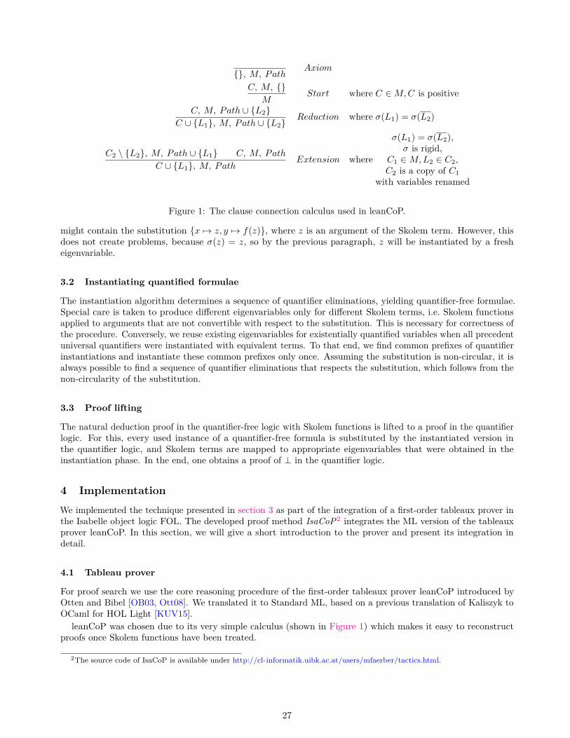
{}, M, PathAxiom

C, M, {}M

Start where C ∈ M,C is positive

C, M, Path ∪ {L2}C ∪ {L1}, M, Path ∪ {L2}

Reduction where σ(L1) = σ(L2)

C2 \ {L2}, M, Path ∪ {L1} C, M, Path

C ∪ {L1}, M, PathExtension where

σ(L1) = σ(L2),σ is rigid,

C1 ∈ M,L2 ∈ C2,C2 is a copy of C1

with variables renamed

Figure 1: The clause connection calculus used in leanCoP.

might contain the substitution {x 7→ z, y 7→ f(z)}, where z is an argument of the Skolem term. However, thisdoes not create problems, because σ(z) = z, so by the previous paragraph, z will be instantiated by a fresheigenvariable.

3.2 Instantiating quantified formulae

The instantiation algorithm determines a sequence of quantifier eliminations, yielding quantifier-free formulae.Special care is taken to produce different eigenvariables only for different Skolem terms, i.e. Skolem functionsapplied to arguments that are not convertible with respect to the substitution. This is necessary for correctness ofthe procedure. Conversely, we reuse existing eigenvariables for existentially quantified variables when all precedentuniversal quantifiers were instantiated with equivalent terms. To that end, we find common prefixes of quantifierinstantiations and instantiate these common prefixes only once. Assuming the substitution is non-circular, it isalways possible to find a sequence of quantifier eliminations that respects the substitution, which follows from thenon-circularity of the substitution.

3.3 Proof lifting

The natural deduction proof in the quantifier-free logic with Skolem functions is lifted to a proof in the quantifierlogic. For this, every used instance of a quantifier-free formula is substituted by the instantiated version inthe quantifier logic, and Skolem terms are mapped to appropriate eigenvariables that were obtained in theinstantiation phase. In the end, one obtains a proof of ⊥ in the quantifier logic.

4 ImplementationWe implemented the technique presented in section 3 as part of the integration of a first-order tableaux prover inthe Isabelle object logic FOL. The developed proof method IsaCoP2 integrates the ML version of the tableauxprover leanCoP. In this section, we will give a short introduction to the prover and present its integration indetail.

4.1 Tableau prover

For proof search we use the core reasoning procedure of the first-order tableaux prover leanCoP introduced byOtten and Bibel [OB03, Ott08]. We translated it to Standard ML, based on a previous translation of Kaliszyk toOCaml for HOL Light [KUV15].

leanCoP was chosen due to its very simple calculus (shown in Figure 1) which makes it easy to reconstructproofs once Skolem functions have been treated.

2The source code of IsaCoP is available under http://cl-informatik.uibk.ac.at/users/mfaerber/tactics.html.

27

4.2 Equality axioms

The core reasoning procedure of leanCoP does not have an inbuilt notion of equality, however the full version ofleanCoP supports equality, by inserting equality axioms into the problem. For that reason, before sending thequantifier logic problem to leanCoP, we prove the following formulae and add them to the original problem:

• reflexivity of equality,• transitivity of equality, and• congruence axioms for every predicate P and every function f appearing in the problem (excluding Skolem

functions and equality itself), such as:

x1 = y1 =⇒ . . . =⇒ xn = yn =⇒ P (x1, . . . , xn) =⇒ P (y1, . . . , yn),x1 = y1 =⇒ . . . =⇒ xn = yn =⇒ f(x1, . . . , xn) = f(y1, . . . , yn).

4.3 Translation to clausal form

To use a refutation-based prover on an Isabelle goal

A1 =⇒ . . . =⇒ An =⇒ C,

it is necessary to first negate the conjecture. To achieve conjecture directed proof search, leanCoP marks theconjecture-related parts of the goal with a special symbol #:

¬C ∨ ¬# =⇒ A1 =⇒ . . . =⇒ An =⇒ # =⇒ ⊥.

Furthermore, it is necessary to translate the goal to a normal form PNF + NNF + CNF. This is achieved usingthe Isabelle simplifier by rewriting with a fixed set of rules such as

¬(a ∧ b) ↔ ¬a ∨ ¬b,(∀x.P (x)) ∨Q ↔ ∀x.(P (x) ∨Q).

The conversion of the goal to normal form is performed as proof steps inside the Isabelle logic, meaning thatevery step is logically verified. In contrast, we do not perform Skolemisation inside the logic, because we do notassume the axiom of choice. Instead, we convert the normal form to an equisatisfiable quantifier-free term byintroducing Skolem functions outside the logic. From the result, we extract the clauses from the quantifier-freeformulae and pass them to leanCoP.

4.4 Proof reconstruction

If leanCoP found a proof (consisting of a substitution and a tableaux proof), IsaCoP extracts all quantifier logicformulae employed in extension steps and instantiates all quantifiers by the proof deskolemisation method shownin section 3. Furthermore, the terms used inside the tableaux proof are converted to terms in the quantifierlogic, replacing Skolem terms by appropriate eigenvariables. Finally, the tableaux proof is converted to a naturaldeduction proof, following the procedure used in MESON proof reconstruction [Har96]. We obtain a proof of ⊥,showing that the negated conjecture is unsatisfiable, thus proving the conjecture.

5 LimitationsIn this section, we shed light on some limitations of our approach, most notably the type of Skolemisation andthe usage of equality.

5.1 Optimised Skolemisation

Table 2: Inner Skolemisation example.

# Quantifier formula Quantifier-free formulat1 ¬P (a, c) ¬P (a, c)t2 ∀w.P (w, c) P (w, c)t3 ∀xy.(P (x, y) ∧ ∃z.¬P (z, y)) P (x, y) ∨ ¬P (f(y), y)

28

We currently use outer Skolemisation, because optimised Skolemisation methods, such as inner Skolemisation,may require creating different eigenvariables for syntactically equivalent Skolem terms. Consider for exampleTable 2. The corresponding natural deduction proof for the quantifier-free formula might look as follows:

1 ¬P (a, c)

2 P (f(c), c)

3.1 P (a, c) ∨ ¬P (f(c), c)

3.2 P (f(c), c) ∨ ¬P (f(c), c)

4 P (a, c)

5 ⊥ ¬E, 4, 1

6 ¬P (f(c), c)

7 P (f(c), c)

8 ⊥ ¬E, 7, 6

9 ¬P (f(c), c)

10 ⊥ ¬E, 2, 9

11 ⊥ ∨E, 3.2, 7–10

12 ⊥ ∨E, 3.1, 4–11

Line 1 to 3.2 contain the instantiated versions of the quantifier-free formulae with Skolem functions. Note thatthe second disjuncts of line 3.1 and 3.2 contain two occurrences of f(c), which in the quantifier logic proof willbe mapped to two different eigenvariables, namely some e1 when x is substituted to a, and some e2 when x issubstituted to f(c). This matters because line 10 depends on the correct instantiation done in line 2, where it isnot immediately clear without an analysis of the refutation whether e1 or e2 should be used in lieu of f(c) toinstantiate ∀w.P (w, c).

5.2 Equality

To use our reconstruction method, proofs in calculi with equality are not allowed to rewrite subterms of Skolemterms. We respect this restriction in our implementation by not generating congruence axioms for Skolemfunctions. To see what can go wrong when Skolem subterms are rewritten, consider the problem

∀x.∃y.P (x, y) ∧ ¬P (x, y) ∧ x = c.

The Skolemised version is∀x.P (x, f(x)) ∧ ¬P (x, f(x)) ∧ x = c,

and instantiating it with a and b yields

P (a, f(a)) ∧ ¬P (a, f(a)) ∧ a = c,

P (b, f(b)) ∧ ¬P (b, f(b)) ∧ b = c.

Assume that the proof shows ⊥ using P (a, f(a)) and ¬P (b, f(b)), rewriting b to a. Reproducing this proof inquantifier logic is difficult, because the Skolem terms do not exist in quantifier logic, so rewriting underneath aSkolem term cannot be simply translated to quantifier logic.

6 Related workThe axiom of choice can be used to represent Skolem functions: Given a formula ∀x.∃y.P (x, y), it can beSkolemised to ∀x.P (x, f(x)), and the Skolem function is then defined to be f = λx.εy.P (x, y) [HB39]. While

29

such reasoning can be in principle expressed in FOL-based logics, it creates an ugly dependency on the axiom ofchoice, which is not assumed in Isabelle/FOL, and certain derived logics such as the Mizar environment do notassume it in general.

Various approaches for reducing the reliance on the axiom of choice are discussed by Blanchette in the section“Skolemization without Choice” of his Ph.D. thesis [Bla12]. In particular, he shows how to simulate Skolemfunctions as (higher-order) schematic functions in Isabelle to reconstruct proofs of the automated theorem proverMetis. Isabelle’s higher-order unifier can then frequently find the function that implements the Skolem function.

Another approach by de Nivelle [dN05] is about the translation of resolution proofs into first-order proofs:He introduces Skolem relations to simulate the effect of Skolem functions. This approach relies on the lesscontroversial definite description operator. Such an operator is however still not provided for any first-order Mizartype [KPU16].

Avigad [Avi03] adds new functions by building finite approximations thereof via a forcing argument. All theseapproaches aim in some or the other way at introducing the Skolem functions in the logic where the proof iscarried out. Our method reconstructs proofs without introducing Skolem functions in the proof assistant.

A more general approach to reconstruct proofs in natural deduction calculi can be achieved by using expansiontrees [Mil83, Pfe87] which implicitly encode quantifier instantiations and also allow reconstruction of proofs thatdo not rely on prenex normal form. We plan to adopt expansion trees in the future.

7 ConclusionWe showed a method to create instances of logic formulae without occurrences of Skolem functions from proofswith Skolem functions. This allows reconstruction of ATP proofs with Skolem functions in first-order logic.Furthermore, we implemented our approach as a proof tactic for Isabelle/FOL, using it to reconstruct proofsfrom a tableaux prover. Further work can be done to improve the tactic, making it a contestant for existingtactics: Treatment of lambda abstractions (which occur in a few places because FOL is encoded as an Isabelleobject logic), e.g. by translating them to combinators, and extension to logics beyond FOL. Furthermore, ourmethod might be usable to reconstruct also proofs from more powerful ATPs, such as E [Sch13] and Vampire[KV13], provided one can obtain suitable substitutions from their proofs and one restricts the usage of equality,see subsection 5.2. In the future, we would like to use expansion trees and to adapt a non-clausal prover [Ott11]for proof search.

AcknowledgementsWe would like to thank Chad Brown for the examples in section 5 and Thomas Powell for the discussions on therole of Skolem functions. This work has been supported by the Austrian Science Fund (FWF) grant P26201.

References[Avi03] Jeremy Avigad. Eliminating definitions and Skolem functions in first-order logic. ACM Trans. Comput.

Log., 4(3):402–415, 2003.

[BKPU16] Jasmin Christian Blanchette, Cezary Kaliszyk, Lawrence C. Paulson, and Josef Urban. Hammeringtowards QED. J. Formalized Reasoning, 9(1):101–148, 2016.

[Bla12] Jasmin C. Blanchette. Automatic Proofs and Refutations for Higher-Order Logic. PhD thesis,Universität München, 2012.

[dN05] Hans de Nivelle. Translation of resolution proofs into short first-order proofs without choice axioms.Inf. Comput., 199(1-2):24–54, 2005.

[Har96] John Harrison. Optimizing proof search in model elimination. In Michael A. McRobbie and John K.Slaney, editors, Automated Deduction - CADE-13, 13th International Conference on AutomatedDeduction, New Brunswick, NJ, USA, July 30 - August 3, 1996, Proceedings, volume 1104 of LectureNotes in Computer Science, pages 313–327. Springer, 1996.

[HB39] David Hilbert and Paul Bernays. Grundlagen der Mathematik II. Springer-Verlag, 1939.

30

[Hur03] Joe Hurd. First-order proof tactics in higher-order logic theorem provers. In Design and Applicationof Strategies/Tactics in Higher Order Logics, number NASA/CP-2003-212448 in NASA TechnicalReports, pages 56–68, 2003.

[KPU16] Cezary Kaliszyk, Karol Pąk, and Josef Urban. Towards a Mizar environment for Isabelle: Foundationsand language. In Jeremy Avigad and Adam Chlipala, editors, Proceedings of the 5th ACM SIGPLANConference on Certified Programs and Proofs, Saint Petersburg, FL, USA, January 20-22, 2016, pages58–65. ACM, 2016.

[KUV15] Cezary Kaliszyk, Josef Urban, and Jirí Vyskocil. Certified connection tableaux proofs for HOL Lightand TPTP. In Xavier Leroy and Alwen Tiu, editors, Proceedings of the 2015 Conference on CertifiedPrograms and Proofs, CPP 2015, Mumbai, India, January 15-17, 2015, pages 59–66. ACM, 2015.

[KV13] Laura Kovács and Andrei Voronkov. First-order theorem proving and Vampire. In Natasha Sharyginaand Helmut Veith, editors, Computer Aided Verification - 25th International Conference, CAV 2013,Saint Petersburg, Russia, July 13-19, 2013. Proceedings, volume 8044 of Lecture Notes in ComputerScience, pages 1–35. Springer, 2013.

[Mil83] Dale A. Miller. Proofs in Higher-Order Logic. PhD thesis, Carnegie Mellon University, 1983.

[NPW02] Tobias Nipkow, Lawrence C. Paulson, and Markus Wenzel. Isabelle/HOL - A Proof Assistant forHigher-Order Logic, volume 2283 of Lecture Notes in Computer Science. Springer, 2002.

[NW01] Andreas Nonnengart and Christoph Weidenbach. Computing small clause normal forms. In John AlanRobinson and Andrei Voronkov, editors, Handbook of Automated Reasoning (in 2 volumes), pages335–367. Elsevier and MIT Press, 2001.

[OB03] Jens Otten and Wolfgang Bibel. leanCoP: lean connection-based theorem proving. J. Symb. Comput.,36(1-2):139–161, 2003.

[Ott08] Jens Otten. leanCoP 2.0 and ileanCoP 1.2: High performance lean theorem proving in classical andintuitionistic logic (system descriptions). In Alessandro Armando, Peter Baumgartner, and GillesDowek, editors, Automated Reasoning, 4th International Joint Conference, IJCAR 2008, Sydney,Australia, August 12-15, 2008, Proceedings, volume 5195 of Lecture Notes in Computer Science, pages283–291. Springer, 2008.

[Ott11] Jens Otten. A non-clausal connection calculus. In Kai Brünnler and George Metcalfe, editors,Automated Reasoning with Analytic Tableaux and Related Methods - 20th International Conference,TABLEAUX 2011, Bern, Switzerland, July 4-8, 2011. Proceedings, volume 6793 of Lecture Notes inComputer Science, pages 226–241. Springer, 2011.

[Pau93] Lawrence C. Paulson. Set theory for verification: I. From foundations to functions. J. Autom.Reasoning, 11(3):353–389, 1993.

[Pau99] Lawrence C. Paulson. A generic tableau prover and its integration with Isabelle. J. UCS, 5(3):73–87,1999.

[Pfe87] Frank Pfenning. Proof Transformations in Higher-Order Logic. PhD thesis, Carnegie Mellon University,1987.

[Sch13] Stephan Schulz. System description: E 1.8. In Kenneth L. McMillan, Aart Middeldorp, and AndreiVoronkov, editors, Logic for Programming, Artificial Intelligence, and Reasoning - 19th InternationalConference, LPAR-19, Stellenbosch, South Africa, December 14-19, 2013. Proceedings, volume 8312 ofLecture Notes in Computer Science, pages 735–743. Springer, 2013.

31

Deduction as a Service

Mohamed Bassem Hassona

German University in Cairomohamed.hassona@student.guc.edu.eg

Stephan Schulz

DHBW Stuttgartschulz@eprover.org

Abstract

We describe a system offering deduction (over a fixed but flexible back-ground theory) as a service, provided to a client via a network con-nection. The deduction server maintains the (potentially) large back-ground knowledge base in a form that makes processing of individualconjectures and queries easy and avoids most of the overhead of read-ing and analyzing large background theories for each individual job.The client connects to the server, can update the background theoryby adding and removing client-side or server-side axiom sets, and askthe server to solve proof problems on its behalf.

This offers several benefits: Preprocessing costs can be amortized overmultiple proof attempts. The user can be isolated from the complexi-ties of a locally installed ATP system (and indeed locally maintainedknowledge bases). Finally, the deduction server can easily offer truestrategy parallelism even with sequential back-end theorem provers.

This paper describes the architecture, the communication protocol, andthe implementation of a deduction server based on E. First experimen-tal results demonstrate the feasibility of the technology and the perfor-mance benefits possible with this approach.

1 Introduction

Classical automated theorem proving has long been concerned with solving individual problems, one at a time.Moreover, problems have often been hand-optimized, either to solve a particular mathematical question, orto analyze and demonstrate the performance of different theorem proving strategies (see e.g. [9]). One of thebest-knows examples is McCune’s formalization and ultimate proof of the Robbins problem [8].

However, in recent years, theorem provers have been used in a very different setting. Users have developedlarge theories, either by large-scale manual coding of knowledge as in Cyc [14] or SUMO [12], by organized

Copyright c© by the paper’s authors. Copying permitted for private and academic purposes.

In: P. Fontaine, S. Schulz, J. Urban (eds.): Proceedings of the 5th Workshop on Practical Aspects of Automated Reasoning(PAAR 2016), Coimbra, Portugal, 02-07-2016, published at http://ceur-ws.org

32

efforts to formalize significant parts of mathematics (e.g. MIZAR [20], or more recently Flyspeck [3]), or fromthe verification of large systems like the sel4 micro-kernel [6]. These theories are typically developed in either aninteractive theorem prover, or in authoring environment like Sigma-KEE [13]. Automated theorem provers canbe used to dispose a significant number of sub-problems that can be translated into first-order logic. Examplesare MizAR for MIZAR and the various “Hammers” for Isabelle [11, 10, 1] and HOL Light/HOL 4 [5, 2].Communication between interactive and local automatic systems is usually via an ad-hoc protocol. As a fallback,some interactive prover also use the TPTP World web service [18] to invoke remotely installed ATP systems.

In these newer use cases, the theorem prover proves and reproves many different theorems over a large andmostly static background theory. Typically, the background theory has thousands to millions of axioms, only asmall fraction of which is used for any given proof. Premise selection techniques [4, 7, 2] enable provers to handlesuch large problems. However, for large problems, parsing and preprocessing takes significant amounts of time.1

In this paper, we suggest a different paradigm. Deduction, over a fixed but flexible base theory, is offered as anetwork service. The deduction server maintains a knowledge base of several pre-loaded background axiomatiza-tion. The user can connect to the server, select specific parts of the knowledge base, add additional assumptions,and then request a proof from the server. The server combines the pre-loaded and pre-indexed backgroundtheory with the new formulas provided by the user, runs several premise selection strategies to generate ATPproblems, and runs several ATP instances with different heuristics to try to solve the problem. If one of theserver processes finds a proof, it is handed back to the client.

This approach has a number of advantages. First, the cost of loading and pre-processing the large backgroundtheory is amortized over many different proof problems. Proofs to individual problems are often found fast andwith low latency. The user can prepare and issue queries from a local desktop, while the deduction server canbe shared by several users and run on powerful server hardware. Indeed, the user does not even need to knowhow to install or invoke ATP systems, since the server can be centrally installed and maintained.

We have developed a suitable communication protocol and implemented a deduction server based on thetheorem prover E[15, 16] and its libraries of data types and algorithms for deduction. First results show that theapproach is feasible, and that the overhead for processing large problems can be significantly reduced. In thefollowing sections we describe the design, architecture, and implementation of the deduction server, and providedata about a first experimental evaluation.

The system is available at http://www.eprover.eu/E-eu/DedServer.html, and will become part of futuredistributions of E.

2 Client-Server Architecture

2.1 Deduction Server

The deduction server is the central component for offering Deduction as a Service. It maintains the current stateof the knowledge base, accepts connections from clients, reads and processes their requests, runs deduction jobson behalf of the clients, and transmits the results back to the client. The main architectural components of theserver are the knowledge base, the TCP interface, the axiom filter, and the execution module.

At start-up, the server starts listening on a user-specified port for incoming TCP connections. Whenever aclient tries to connect to the server on that port, a process is forked from the main process to serve the client.The server can thus handle several different connections at the same time, and each client is completely isolatedfrom other clients connected to the server.

The client interacts with the server using the protocol specified in section 2.3. The server implements a typicalread-execute-print loop, accepting commands from the client, executing them, and sending the results back tothe client. The client can upload axiom sets, remove them, and query the server for proofs and answers (i.e.instantiations of variables that make an existentially quantified query formula true [19]).

Whenever the client uploads a set of axioms, the server parses the axioms, adds them to various indexes usefulfor axiom selection/pruning methods, and adds them to the in-memory knowledge base. However, these uploadedaxiom sets will not automatically be used by each proof attempt, but only when the client has also activated (orstaged) the particular set in the current session. Thus, the server maintains a pre-indexed, ready-to-use libraryof axiom sets. In addition to axiom sets uploaded by the client, the server can also offer access to axiom sets

1As an example, E takes around 54 seconds (on a system with a 4 GHz Intel i7 and a fast SSD) just to parse the TPTP problemCSR073+6.p, a first-order problem based on OpenCyc with nearly 3.5 million axioms and taking up 480 MB. Indexing for SInE axiomselection takes a further 2 seconds, while more than half of successful proof attempts need less than 1 second.

33

Figure 1: The Deduction Server Architecture

stored in a server-side library on disk. Axioms loaded by the server on start-up are available to all users, whileaxiom sets added by a user during a session are currently only available in that session.

After the client chooses some axiom sets to be used in the proof search, it can start querying the server.The query consists of optional query-specific axioms and a conjecture. These additional formulas are discardedimmediately after the query has been processed. The server adds the new axiom set to the currently staged partof the knowledge base and hands the problem to the axiom filter. The axiom filter module applies one or multipledifferent relevancy pruning strategies to the extended knowledge base. Each of the pruning strategies producesone much smaller proof problem. The pruned problems are passed to the execution module, which starts severalinstances of E in parallel and monitors their success or failure. Whenever one of the running E instances finds aproof for the conjecture, the other instances are stopped and the proof is returned back to the user. Currently,all instanced of E use its conventional automatic mode, and rely on the different pruning strategies to providediversity for the proof attempt.

The rough architecture of the deduction server is shown in Figure 1.The deduction server is written in C and integrated with the E distribution. It uses the E libraries and data

types to parse and represent logical formulas, to maintain and process first order knowledge bases, and to performaxiom selection.

2.2 User client

The E distribution includes a small Python client called “enetcat.py”, which can be used to interact with theserver. The client is intended as a reference implementation, to demonstrate the interactions with the server andenable other developers to use it as a model for interfacing the server with other systems.

The client requires the address and the port of the deduction server as arguments. It opens a TCP connectionto the server and then reads the user’s commands from “stdin”, communicates them to the server, and printsthe output back to “stdout”.

In addition to encoding the plain text commands into the distinct length-delimited TCP messages expectedby the server, the client offers two convenience features. First, it offers command line editing. Secondly, it locallyexpands TPTP style include commands for formula sets to be uploaded to the server. This makes uploading

34

of even large axioms sets plausible and convenient.The current client is tailored towards command-line users. However, the protocol is simple enough to be

implemented in a few lines of code in nearly any modern programming language, making other clients, inparticular a web-based client, easily possible.

2.3 Communication Protocol

As mentioned before, the communication between the server and the client is done over TCP to ensure reliability.TCP messages between the server and the client are encoded in a way to ease the communication between them.Each TCP messages starts with 4 bytes containing the length of the messages, including those 4 bytes, followedby the actual message. The commands themselves are plain, human-readable ASCII text.

We describe the protocol for communication between the server and the client using a running example.We assume that the connection has already been established and all messages are encoded as described in theprevious paragraph.

The first section of the session uploads two small axiom sets to the server.

1 ADD axiom_set1

2 fof(inp1,axiom,(subclass(a,b))).

3 fof(inp2,axiom,(subclass(b,c))).

4 GO

5 >205 ok : added

67 ADD axiom_set2

8 fof(inp3,axiom,((subclass(X,Y) & subclass(Y,Z)) => subclass(X,Z))).

9 GO

10 >205 ok : added

Each of the “ADD . . . GO” blocks upload one named set of axioms to the system. Axioms uploaded are parsedand stored in the memory of the server, but are not automatically included in future proof attempts. The serverresponds with the success status of each command’s execution.

1 STAGE axiom_set1

2 >201 ok : staged

34 LIST

5 >Staged :

6 > axiom_set1

7 >Unstaged :

8 > axiom_set2

9 >On Disk :

10 > test.p

11 >200 ok : success

1213 STAGE axiom_set2

14 >201 ok : staged

To select axiom sets for future proof attempts, we use the “STAGE” command. It marks the named axiom setas active for later proof attempts. The “LIST” command provides the status of all axiom sets currently knownto the server. Possible states are Staged, Unstaged (but in memory and pre-indexed for axiom selection), and OnDisk, i.e. known to the server, but not loaded or indexed. Server-side axiom sets can be loaded into the server’smemory using the “LOAD” command.

1 RUN job1

2 fof(inp4,conjecture,(subclass(a,c))).

3 GO

4 # Pid: 27988

5 # Auto-Mode selected heuristic G_E___208_C18_F1_SE_CS_SP_PS_S0Y

6 # and selection function SelectMaxLComplexAvoidPosPred.

7 #

35

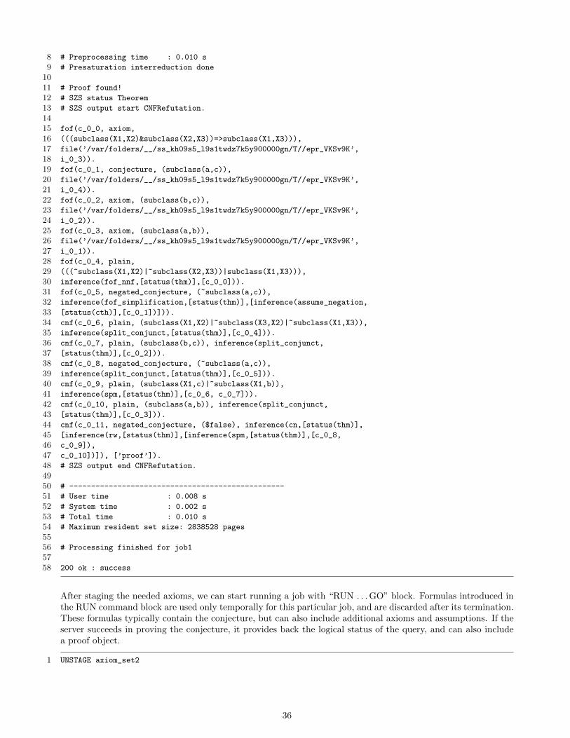
8 # Preprocessing time : 0.010 s

9 # Presaturation interreduction done

1011 # Proof found!

12 # SZS status Theorem

13 # SZS output start CNFRefutation.

1415 fof(c_0_0, axiom,

16 (((subclass(X1,X2)&subclass(X2,X3))=>subclass(X1,X3))),

17 file(’/var/folders/__/ss_kh09s5_l9s1twdz7k5y900000gn/T//epr_VKSv9K’,

18 i_0_3)).

19 fof(c_0_1, conjecture, (subclass(a,c)),

20 file(’/var/folders/__/ss_kh09s5_l9s1twdz7k5y900000gn/T//epr_VKSv9K’,

21 i_0_4)).

22 fof(c_0_2, axiom, (subclass(b,c)),

23 file(’/var/folders/__/ss_kh09s5_l9s1twdz7k5y900000gn/T//epr_VKSv9K’,

24 i_0_2)).

25 fof(c_0_3, axiom, (subclass(a,b)),

26 file(’/var/folders/__/ss_kh09s5_l9s1twdz7k5y900000gn/T//epr_VKSv9K’,

27 i_0_1)).

28 fof(c_0_4, plain,

29 (((~subclass(X1,X2)|~subclass(X2,X3))|subclass(X1,X3))),

30 inference(fof_nnf,[status(thm)],[c_0_0])).

31 fof(c_0_5, negated_conjecture, (~subclass(a,c)),

32 inference(fof_simplification,[status(thm)],[inference(assume_negation,

33 [status(cth)],[c_0_1])])).

34 cnf(c_0_6, plain, (subclass(X1,X2)|~subclass(X3,X2)|~subclass(X1,X3)),

35 inference(split_conjunct,[status(thm)],[c_0_4])).

36 cnf(c_0_7, plain, (subclass(b,c)), inference(split_conjunct,

37 [status(thm)],[c_0_2])).

38 cnf(c_0_8, negated_conjecture, (~subclass(a,c)),

39 inference(split_conjunct,[status(thm)],[c_0_5])).

40 cnf(c_0_9, plain, (subclass(X1,c)|~subclass(X1,b)),

41 inference(spm,[status(thm)],[c_0_6, c_0_7])).

42 cnf(c_0_10, plain, (subclass(a,b)), inference(split_conjunct,

43 [status(thm)],[c_0_3])).

44 cnf(c_0_11, negated_conjecture, ($false), inference(cn,[status(thm)],

45 [inference(rw,[status(thm)],[inference(spm,[status(thm)],[c_0_8,

46 c_0_9]),

47 c_0_10])]), [’proof’]).

48 # SZS output end CNFRefutation.

4950 # -------------------------------------------------

51 # User time : 0.008 s

52 # System time : 0.002 s

53 # Total time : 0.010 s

54 # Maximum resident set size: 2838528 pages

5556 # Processing finished for job1

5758 200 ok : success

After staging the needed axioms, we can start running a job with “RUN . . . GO” block. Formulas introduced inthe RUN command block are used only temporally for this particular job, and are discarded after its termination.These formulas typically contain the conjecture, but can also include additional axioms and assumptions. If theserver succeeds in proving the conjecture, it provides back the logical status of the query, and can also includea proof object.

1 UNSTAGE axiom_set2

36

CSR025+6.p CSR026+6.p CSR027+6.p CSR028+6.p CSR029+6.p CSR030+6.p

CSR031+6.p CSR032+6.p CSR033+6.p CSR034+6.p CSR035+6.p CSR036+6.p

CSR037+6.p CSR038+6.p CSR039+6.p CSR040+6.p CSR041+6.p CSR042+6.p

CSR043+6.p CSR044+6.p CSR045+6.p CSR046+6.p CSR047+6.p CSR048+6.p

CSR049+6.p CSR050+6.p CSR051+6.p CSR052+6.p CSR053+6.p CSR054+6.p

CSR055+6.p CSR056+6.p CSR057+6.p CSR058+6.p CSR059+6.p CSR060+6.p

CSR061+6.p CSR062+6.p CSR063+6.p CSR064+6.p CSR065+6.p CSR066+6.p

CSR067+6.p CSR068+6.p CSR069+6.p CSR070+6.p CSR071+6.p CSR072+6.p

CSR073+6.p CSR074+6.p CSR111+6.p

Figure 2: List of problems used in the evaluation

2 >202 ok : unstaged

34 REMOVE axiom_set2

5 >203 ok : removed

67 DOWNLOAD axiom_set1

8 >fof(inp1,axiom,(subclass(a,b))).

9 >fof(inp2,axiom,(subclass(b,c))).

10 >204 ok : downloaded

1112 RUN job2

13 fof(inp4,conjecture,(subclass(a,c))).

14 GO

15 # Processing started for job2

16 # SZS status GaveUp for job2

1718 # Processing finished for job2

1920 200 ok : success

Axiom sets can also be “UNSTAGE”d or “REMOVE”d completely from the system. Axiom sets can be retrievedfrom the server using the “DOWNLOAD” command. The example shows how we remove one of the axiom setsand re-run the job. Without the necessary axioms, the proof is not found.

3 Evaluation

For the experimental evaluation, we selected a set of large problems with a common axiomatization from theTPTP library [17], version 6.0.0. In particular, we used all problems that include the axiom set CSR002+5.ax, atranslation of the OpenCyc knowledge base into first-order logic [14]. The axiom set contains 3 341 983 axiomsand occupies about 479 megabytes disk space in TPTP format. It is used by 51 problems, each of which combinesit with a single unique conjecture. See Figure 2 for the list of problems.

To illustrate the comparative performance of the service model and the conventional one-problem-at-a-timemodel, we configured both versions to run exactly the same problems with exactly the same pruning parametersand E’s sequential automatic mode. In particular, the server did not employ any strategy parallelism in pruningor search, but rather selected the same search strategy than the stand-alone prover for each a given problem.

The systems were given a time limit of 30 seconds for actual proof search, in addition to the time taken forparsing and axiom selection for the standalone version (about 110 seconds per problem on this hardware, withsome variation). Memory was limited to 1024MB. Tests were performed on a virtualized server with 8 2.6 GHzIntel CPUs, of which only one was effectively utilized by our test setup. With this configuration, both setupssolved 41 of the 51 problems.

We recorded the time taken after 5, 10, 20, 30, 40 and all 51 problems.The results in Figure 3 show the difference between the single strategy server mode and the conventional

prover. The figure shows the accumulated wall-clock time over the number of problems for which a proof wasattempted. In the conventional case, the prover has to parse and index the axiom set for each proof attempt.In the deduction server, the axioms are parsed and indexed for axiom selection only once. The are then kept in

37

Figure 3: Benchmarking Results

the server’s memory and multiple queries can be executed against this axiom set. Thus, the pre-processing timeof each problem in the single strategy server mode is amortized over multiple runs.

4 Conclusion

We have described the first implementation of a Deduction Server and have introduced a communication protocolthat supports remote reasoning over largely fixed but flexible domains as a service. Our results shows that thededuction server, even if configured for identical pruning and search strategies, improves the run time for sets ofrelated problems by a significant amount, due to the amortization of costs for parsing and the indexing neededfor axiom selection. This clearly shows that the approach is feasible and has promise even if looking at it onlyfrom a performance point of view.

In addition to these performance benefits, having a formal protocol to communicate with the prover over thenet makes integrating it with other applications much easier. Having access to a remotely running prover is a winfor those who can’t install provers locally, e.g. for OS compatibility issues or due to insufficient local computingresources.

Future work includes improved multi-user support, in particular controlling both access, but also the resources,such as CPU time and memory, allocated for each user. Another important step would be the integration ofmultiple deduction systems in the back-end, to improve overall performance. This would offer a single interfaceto potentially very diverse deduction systems.

Finally, the Deduction Server can be extended to a cluster of servers, to offer real scalable deduction as aservice. In the simplest version, a single head node accepts and processes user commands, pre-processes theproblems, and distributes the deduction jobs to different servers. An even more scalable version would maintaindifferent user sessions with the current axiomatization on dedicated machines, so that axiom selection can alsobe distributed.

References

[1] Sascha Bohme and Tobias Nipkow. Sledgehammer: Judgement Day. In Jurgen Giesel and Reiner Hahnle,editors, Proc. of the 5th IJCAR, Edinburgh, volume 6173 of LNAI, pages 107–121. Springer, 2010.

38

[2] Thibault Gauthier and Cezary Kaliszyk. Premise Selection and External Provers for HOL4. In Proceedingsof the 2015 Conference on Certified Programs and Proofs, pages 49–57, New York, NY, USA, 2015. ACM.

[3] Thomas C. Hales, John Harrison, Sean McLaughlin, Tobias Nipkow, Steven Obua, and Roland Zumkeller.A revision of the proof of the Kepler conjecture. In Jeffrey C. Lagarias, editor, The Kepler Conjecture,pages 341–376. Springer, 2011.

[4] Krystof Hoder and Andrei Voronkov. Sine Qua Non for Large Theory Reasoning. In Nikolaj Bjørner andViorica Sofronie-Stokkermans, editors, Proc. of the 23rd CADE, Wroclav, volume 6803 of LNAI, pages299–314. Springer, 2011.

[5] Cezary Kaliszyk and Josef Urban. Learning-assisted automated reasoning with Flyspeck. Journal of Auto-mated Reasoning, 53(2):173–213, 2014.

[6] Gerwin Klein, Kevin Elphinstone, Gernot Heiser, June Andronick, David Cock, Philip Derrin, DhammikaElkaduwe, Kai Engelhardt, Rafal Kolanski, Michael Norrish, Thomas Sewell, Harvey Tuch, and SimonWinwood. seL4: Formal verification of an OS kernel. In Proc. of the 22nd ACM Symposium on Principlesof Operating Systems (SOSPS), Big Sky, Montana, USA, October 2009. ACM.

[7] Daniel Kuhlwein, Twan van Laarhoven, Evgeni Tsivtsivadze, Josef Urban, and Tom Heskes. Overviewand evaluation of premise selection techniques for large theory mathematics. In Bernhard Gramlich, UlrikeSattler, and Dale Miller, editors, Proc. of the 6th IJCAR, Manchester, volume 7364 of LNAI, pages 378–392.Springer, 2012.

[8] William McCune. Solution of the Robbins problem. Journal of Automated Reasoning, 19(3):263–276, 1997.

[9] W.W. McCune. 33 Basic Test Problems: A Practical Evaluation of Some Paramodulation Strategies. InR. Veroff, editor, Automated Reasoning and its Applications: Essays in Honor of Larry Wos, chapter 5,pages 71–114. MIT Press, 1997.

[10] Jia Meng and Lawrence C. Paulson. Translating higher-order clauses to first-order clauses. Journal ofAutomated Reasoning, 40(1):35–60, 2008.

[11] Jia Meng and Lawrence C. Paulson. Lightweight relevance filtering for machine-generated resolution prob-lems. Journal of Applied Logics, 7(1):41–57, 2009.

[12] Adam Pease, Ian Niles, and John Li. The Suggested Upper Merged Ontology: A Large Ontology for theSemantic Web and its Applications. In Working Notes of the AAAI-2002 Workshop on Ontologies and theSemantic Web, 2002.

[13] Adam Pease and Stephan Schulz. Knowledge Engineering for Large Ontologies with Sigma KEE 3.0. InStephane Demri, Deepak Kapur, and Christoph Weidenbach, editors, Proc. of the 7th IJCAR, Vienna,volume 8562 of LNAI, pages 519–525. Springer, 2014.

[14] Deepak Ramachandran, Pace Reagan, and Keith Goolsbey. First-orderized ResearchCyc: Expressivenessand Efficiency in a Common Sense Knowledge Base. In Pavel Shvaiko, editor, Proc. of the AAAI Workshopon Contexts and Ontologies: Theory, Practice and Applications (C&O-2005), 2005.

[15] S. Schulz. E – A Brainiac Theorem Prover. Journal of AI Communications, 15(2/3):111–126, 2002.

[16] Stephan Schulz. System Description: E 1.8. In Ken McMillan, Aart Middeldorp, and Andrei Voronkov,editors, Proc. of the 19th LPAR, Stellenbosch, volume 8312 of LNCS. Springer, 2013.

[17] Geoff Sutcliffe. The TPTP Problem Library and Associated Infrastructure: The FOF and CNF Parts,v3.5.0. Journal of Automated Reasoning, 43(4):337–362, 2009.

[18] Geoff Sutcliffe. The TPTP World - infrastructure for automated reasoning. In E. Clarke and A. Voronkov,editors, Proc. of the 16th LPAR, Dakar, number 6355 in LNAI, pages 1–12. Springer, 2010.

[19] Geoff Sutcliffe, Mark Stickel, Stephan Schulz, and Josef Urban. Answer Extraction for TPTP. http:

//www.cs.miami.edu/~tptp/TPTP/Proposals/AnswerExtraction.html. (acccessed 2013-07-08).

39

[20] Andrzej Trybulec and Howard A. Blair. Computer assisted reasoning with MIZAR. In Proc. of the 9thIJCAI, Los Angeles, volume 85, pages 26–28. Morgan Kaufmann, 1985.

40

TH1: The TPTP Typed Higher-Order Form

with Rank-1 Polymorphism

Cezary KaliszykUniversity of Innsbruck, Austria

Geoff SutcliffeUniversity of Miami, USA

Florian RabeJacobs University Bremen, Germany

Abstract

The TPTP world is a well established infrastructure that supports re-search, development, and deployment of Automated Theorem Prov-ing (ATP) systems for classical logics. The TPTP language is oneof the keys to the success of the TPTP world. Originally the TPTPworld supported only first-order clause normal form (CNF). Over theyears support for full first-order form (FOF), monomorphic typed first-order form (TF0), rank-1 polymorphic typed first-order form (TF1),and monomorphic typed higher-order form (TH0) have been added.The TF0, TF1, and TH0 languages also include constructs for arith-metic. This paper introduces the TH1 form, an extension of TH0 withTF1-style rank-1 polymorphism. TH1 is designed to be easy to processby existing reasoning tools that support ML-style polymorphism. Thehope is that TH1 will be implemented in many popular ATP systemsfor typed higher-order logic.

1 Introduction

The TPTP world [18] is a well established infrastructure that supports research, development, and deployment ofAutomated Theorem Proving (ATP) systems for classical logics. The TPTP world includes the TPTP problemlibrary, the TSTP solution library, the TMTP model library, standards for writing ATP problems and reportingATP solutions, tools and services for processing ATP problems and solutions, and it supports the CADE ATPSystem Competition (CASC). Various parts of the TPTP world have been deployed in a range of applications,in both academia and industry. The web page http://www.tptp.org provides access to all components.

The TPTP language is one of the keys to the success of the TPTP world. The language is used for writingboth TPTP problems and TSTP solutions, which enables convenient communication between different systemsand researchers. Originally the TPTP world supported only first-order clause normal form (CNF) [21]. Overthe years support for full first-order form (FOF) [17], monomorphic typed first-order form (TF0) [20], rank-1polymorphic typed first-order form (TF1) [3], and monomorphic typed higher-order form (TH0) [19] have beenadded. The TF0, TF1, and TH0 languages also include constructs for arithmetic. These extensions provideorthogonal features that are natural to combine. In fact, several users have already used ad-hoc definitions ofcombined languages, and [9] already suggested a systematic way to combine specifications.

This paper introduces the TH1 format, a combination of the features of TH0 with TF1-style rank-1 polymor-phism. TH1 is designed to be easy to process by existing reasoning tools that support ML-style polymorphism.

Copyright c© by the paper’s authors. Copying permitted for private and academic purposes.

In: P. Fontaine, S. Schulz, J. Urban (eds.): Proceedings of the 5th Workshop on Practical Aspects of Automated Reasoning(PAAR 2016), Coimbra, Portugal, 02-07-2016, published at http://ceur-ws.org

41

It opens the door to useful middleware, such as monomorphizers and other translation tools that encode poly-morphism in FOF or TH0. Many existing ATP and ITP systems for higher-order logic already implement somekind of polymorphism. TH1 has been designed in interaction with those systems’ developers, and can providean interoperability layer for their systems. The hope is that TH1 will be implemented in many popular ATPsystems for typed higher-order logic.

Figure 1 shows the relationships between the various TPTP language forms, leading to TH1. TH1 combinestwo existing orthogonal extensions to the basic FOF language: the polymorphic TF1 and the higher-order TH0.1

Therefore, this paper first presents the preceding TF0, TF1, and TH0 forms, whose features are then inheritedin the TH1 form.

The remainder of this paper is organized as follows: Section 2 introduces the generic TPTP language, with abrief review of the well-known first-order form. Sections 2.1 and 2.2 describe the monomorphic and polymorphictyped first-order forms, and Section 2.3 describes the monomorphic typed higher-order form. Sections 3 and 4 arethe heart of the paper, describing the syntax and semantics of the polymorphic higher-order form respectively.Section 5 explains the LF-based type checking system for the typed languages. Section 6 concludes.

CNF

FOF

TF0

TF1

TH0

TH1Figure 1: The DAG of TPTP Language Forms

2 The TPTP Language

The TPTP language is a human-readable, easily machine-parsable, flexible and extensible language, suitable forwriting both ATP problems and solutions. The top level building blocks of the TPTP language are annotatedformulae. An annotated formula has the form:

language(name, role, formula, [source, [useful info]]).The languages supported are clause normal form (cnf), first-order form (fof), typed first-order form (tff), andtyped higher-order form (thf). The role, e.g., axiom, lemma, conjecture, defines the use of the formula in anATP system. In the formula, terms and atoms follow Prolog conventions, i.e., functions and predicates startwith a lowercase letter or are ’single quoted’, variables start with an uppercase letter, and all contain onlyalphanumeric characters and underscore. The TPTP language also supports interpreted symbols, which eitherstart with a $, or are composed of non-alphanumeric characters, e.g., the truth constants $true and $false,and integer/rational/real numbers such as 27, 43/92, -99.66. The basic logical connectives are !, ?, ~, |, &, =>,<=, <=>, and <~>, for ∀, ∃, ¬, ∨, ∧, ⇒, ⇐, ⇔, and ⊕ respectively. Equality and inequality are expressed as theinfix operators = and !=. An example annotated first-order formula, supplied from a file, is:

fof(union,axiom,

( ! [X,A,B] :

( member(X,union(A,B))

<=> ( member(X,A)

| member(X,B) ) )

file(’SET006+0.ax’,union),

[description(’Definition of union’), relevance(0.9)]).

1Note that while TH1 adopts features of TF1, TH0 is independent of TF0.

42

2.1 The Monomorphic Typed First-order Form TF0

TF0 extends the basic FOF language with types and type declarations. Every function and predicate symbol isdeclared before its use, with a type signature that specifies the types of the symbol’s arguments and result.

TF0 types τ have the following forms:

• the predefined types $i for ι (individuals) and $o for o (booleans);

• the predefined arithmetic types $int (integers), $rat (rationals), and $real (reals);

• user-defined types (constants).

User-defined types are declared (before their use) to be of the kind $tType, in annotated formulae with a type

role – see Figure 2 for examples. All symbols share the same namespace; in particular, a type cannot have thesame name as a function or predicate symbol.

TF0 type signatures ς have the following forms:

• individual types τ ;

• (τ1 * · · · * τn) > τ for n > 0, where τi are the argument types, and τ is the result type. Argument typesand the result type for a function cannot be $o, and the result type for a predicate must be $o. If n = 1the parentheses are omitted.

The type signatures of uninterpreted symbols are declared like types, in annotated formulae with a type role –see Figure 2 for examples. The type of = is ad hoc polymorphic over all types except $o, with both argumentshaving the same type and the result type being $o. The types of arithmetic predicates and functions are ad hocpolymorphic over the arithmetic types; see [20] for details.

In logical formulae the arguments to functions and predicates must respect the symbol’s type signature.Variables must be typed in their quantification, and used accordingly. For example, in Figure 2 the predicatechased is declared to have the type signature

(dog * cat) > $o

so an example of a well-formed formula is! [X: dog] : chased(X,garfield)

because X is of type dog and garfield is of type cat.Figure 2 illustrates some TF0 formulae, whose conjecture can be proved from the axioms (it is the TPTP

problem PUZ130 1.p).

2.2 The Polymorphic Typed First-order Form TF1

TF1 extends TF0 with (user-defined) type constructors, type variables, polymorphic symbols, and one new binder.

TF1 types τ have the following forms:

• the predefined types $i and $o;

• the predefined arithmetic types $int, $rat, and $real;

• user-defined n-ary type constructors applied to n type arguments;

• type variables, which must be quantified by !> – see the type signature forms below.

Type constructors are declared (before their use) to be of the kind ($tType * · · · * $tType) > $tType, inannotated formulae with a type role. The type constructor’s arity is the number of “$tType”s before the >. Ifthe arity is zero the > is omitted, and the type constructor is a monomorphic user-defined type constant as inTF0, else it is polymorphic. If the arity is less than two the parentheses are omitted. In the example of Figure 3,cup of is a unary type constructor that is is used to construct the type cup of(beverage)).

TF1 type signatures ς have the following forms:

43

%------------------------------------------------------------------------------

tff(animal_type,type,( animal: $tType )).

tff(cat_type,type,( cat: $tType )).

tff(dog_type,type,( dog: $tType )).

tff(human_type,type,( human: $tType )).

tff(cat_to_animal_type,type,( cat_to_animal: cat > animal )).

tff(dog_to_animal_type,type,( dog_to_animal: dog > animal )).

tff(garfield_type,type,( garfield: cat )).

tff(odie_type,type,( odie: dog )).

tff(jon_type,type,( jon: human )).

tff(owner_of_type,type,( owner_of: animal > human )).

tff(chased_type,type,( chased: ( dog * cat ) > $o )).

tff(hates_type,type,( hates: ( human * human ) > $o )).

tff(human_owner,axiom,(

! [A: animal] :

? [H: human] : H = owner_of(A) )).

tff(jon_owns_garfield,axiom,(

jon = owner_of(cat_to_animal(garfield)) )).

tff(jon_owns_odie,axiom,(

jon = owner_of(dog_to_animal(odie)) )).

tff(jon_owns_only,axiom,(

! [A: animal] :

( jon = owner_of(A)

=> ( A = cat_to_animal(garfield) | A = dog_to_animal(odie) ) ) )).

tff(dog_chase_cat,axiom,(

! [C: cat,D: dog] :

( chased(D,C)

=> hates(owner_of(cat_to_animal(C)),owner_of(dog_to_animal(D))) ) )).

tff(odie_chased_garfield,axiom,(

chased(odie,garfield) )).

tff(jon_hates_jon,conjecture,(

hates(jon,jon) )).

%------------------------------------------------------------------------------

Figure 2: TF0 Formulae

44

• individual types τ ;

• (τ1 * · · · * τn) > τ for n > 0, where τi are the argument types and τ is the result type (with the samecaveats as for TF0);

• !>[α1: $tType, . . . ,αn: $tType]: ς for n > 0, where α1, . . . , αn are distinct type variables and ς is a typesignature.

The binder !> in the last form denotes universal quantification in the style of λΠ calculi. It is only used atthe top level in polymorphic type signatures. All type variables must be of type $tType; more complex typevariables, e.g., $tType > $tType are beyond rank-1 polymorphism. In the example of Figure 3, the type signaturefor mixture is polymorphic. As in TF0, arithmetic symbols and equality are ad hoc polymorphic.

Type variables that are bound by !> without occurring in a type signature’s body, e.g., as in thelast example, are called phantom type variables. These make it possible to specify operations and rela-tions directly on types and provide a convenient way to encode type classes. For example, a polymor-phic propositional constant is linear can be declared with the type signature !>[A : $tType]: $o, andused as a guard to restrict the axioms specifying that a binary predicate less eq with the type signature!>[A: $tType]: ((A * A) > $o) is a linear order to those types that satisfy the is linear predicate, i.e., aformula of the form ! [A: $tType] : ( (is linear @ A) => (axiom about less eq)).

In logical formulae the application of symbols must respect the symbol’s type signature. Addi-tionally, every use of a polymorphic symbol (except ad hoc polymorphic arithmetic and equality sym-bols) must explicitly specify the type instance. A function or predicate symbol with a type signature!>[α1: $tType, . . . ,αm: $tType]: ((τ1 * · · · > τn > τ) must be applied to m type arguments and n termarguments. For example, in Figure 3 below, the type contructor cup of, the function full cup, the functionmixture, and the predicate help stay awake, are declared to have the type signatures

$tType > $tType

beverage > cup of(beverage)

!>[BeverageOrSyrup: $tType] : ((BeverageOrSyrup * syrup) > BeverageOrSyrup)

cup of(beverage) > $o

so an example of a well-formed formula is! [S: syrup] : help stay awake(full cup(mixture(beverage,coffee,S)))

because beverage provides the one type argument for mixture, coffee is of that type, S is of type syrup, andthe result type is beverage as required by full cup, whose whose result type is in turn cup of(beverage) asrequired by help stay awake. As TF1 is rank-1 polymorphic, the type arguments must be actual types; inparticular $tType and !>-binders cannot occur in type arguments of polymorphic symbols.

Figure 3 illustrates some TF1 formulae, whose conjecture can be proved from the axioms (it is a variant ofthe TPTP problem PUZ139 1.p).

2.3 The Monomorphic Typed Higher-order Form TH0

TH0 extends FOF with higher-order notions, including adoption of curried form for type declarations, lambdaterms (with a lambda binder), symbol application, and two other new binders.

TH0 types τ have the following forms:

• the predefined types $i and $o;

• the predefined arithmetic types $int, $rat, and $real;

• user-defined types (constants);

• (τ1 > · · · > τn > τ) for n > 0, where τi are the argument types and τ is the result type.

TH0 type signatures ς have the following forms:

• individual types τ .

45

%------------------------------------------------------------------------------

ff(beverage_type,type,( beverage: $tType )).

tff(syrup_type,type,( syrup: $tType )).

tff(cup_of_type,type,( cup_of: $tType > $tType )).

tff(full_cup_type,type,( full_cup: beverage > cup_of(beverage) )).

tff(coffee_type,type,( coffee: beverage )).

tff(vanilla_type,type,( vanilla: syrup )).

tff(caramel_type,type,( caramel: syrup )).

tff(help_stay_awake_type,type,( help_stay_awake: cup_of(beverage) > $o )).

tff(mixture_type,type,(

mixture: !>[BeverageOrSyrup: $tType] :

( ( BeverageOrSyrup * syrup ) > BeverageOrSyrup ) )).

%----Coffee keeps you awake

tff(mixture_of_coffee_help_stay_awake,axiom,(

! [S: syrup] : help_stay_awake(full_cup(mixture(beverage,coffee,S))) )).

%----Coffee mixed with a syrup or two helps you stay awake

tff(syrup_coffee_help_stay_awake,conjecture,(

help_stay_awake(full_cup(

mixture(beverage,coffee,mixture(syrup,caramel,vanilla)))) )).

%------------------------------------------------------------------------------

Figure 3: TF1 Formulae

The (τ1 > · · · > τn > τ) form is promoted to be a type in TH0 (and TH1) forms, so that variables in formulae canbe quantified as function types. The curried form means that TH0 provides the possibility of partial application.As in TF0, arithmetic symbols and equality are ad hoc polymorphic.

The new binary connective @ represents application (explicit use of @ is required – symbols cannot simplybe juxtaposed) – see Figure 4 for examples. There are three new binders: ^, @+, and @-, for λ, ε (indefinitedescription, aka choice), and ι (definite description). Use of all the connectives as terms is also supported – thisis quite straightforward because connectives are equivalent (in Henkin semantics - see below) to correspondinglambda abstractions. The arithmetic predicates and functions, and the equality operator, can also be used asterms, but must be applied to a term of a known type (which must be an arithmetic type for the arithmeticsymbols). This formula illustrates the use of conjunction as a term, in a definition of false,

thf(and_false,definition,(

( ( & @ $false )

= ( ^ [Q: $o] : $false ) ) )).

In logical formulae the application of symbols must respect the symbol’s type signature. For example, inFigure 4 the symbols mix and hot are declared to have the type signatures

beverage > syrup > beverage

beverage > $o

so an example of a well-formed formula is! [S: syrup] : (hot @ (mix @ coffee @ S))

because S is of type syrup, coffee is of type beverage, and mix the result type is beverage as required byhot. Partial application results in a lambda term. For example, mix @ coffee produces a lambda term of typesyrup > beverage.

Figure 4 illustrates some TH0 formulae, whose conjecture can be proved from the axioms (it is a variant ofthe TPTP problem PUZ140^1.p). The following formula illustrates the definite description binder (the indefiniteand definite description binders are not used in Figure 4) for a set whose elements of type $i are all equal,

thf(one_set,axiom,

( ! [Z: $i] : ( ( p @ Z ) => ( Z = y ) )

=> ( ( @-[X: $i] : ( p @ X ) ) = y ) )).

The semantics for TH0 is Henkin semantics with choice (Henkin semantics by definition also includes Booleanand functional extensionality) [1, 8].

46

%------------------------------------------------------------------------------

thf(syrup_type,type,( syrup: $tType )).

thf(beverage_type,type,( beverage: $tType )).

thf(coffee_type,type,( coffee: beverage )).

thf(mix_type,type,( mix: beverage > syrup > beverage )).

thf(coffee_mixture_type,type,( coffee_mixture: syrup > beverage )).

thf(hot_type,type,( hot: beverage > $o )).

%----The mixture of coffee and something

thf(coffee_mixture_definition,definition,

( coffee_mixture = ( mix @ coffee ) )).

%----Any coffee mixture is hot coffee

thf(coffee_and_syrup_is_hot_coffee,axiom,(

! [S: syrup] : ( ( (coffee_mixture @ S) = coffee )

& ( hot @ ( coffee_mixture @ S ) )) )).

%----There is some mixture of coffee and any syrup which is hot coffee

thf(there_is_hot_coffee,conjecture,(

? [SyrupMixer: syrup > beverage] :

! [S: syrup] :

? [B: beverage] :

( ( B = ( SyrupMixer @ S ) ) & ( B = coffee ) & ( hot @ B ) ) )).

%------------------------------------------------------------------------------

Figure 4: TH0 Formulae

3 The TH1 Syntax

TH1 combines the higher-order features of TH0 (curried form, lambda terms, description, partial application)with the polymorphic features of TF1 (type constructors, type variables, polymorphic symbols). TH1 also addsfive new polymorphic constants.

TH1 types τ have the following forms:

• the predefined types $i and $o;

• user-defined n-ary type constructors applied to n type arguments;

• type variables (which must be quantified by !>);

• (τ1 > · · · > τn > τ) for n > 0, where τi are the argument types and τ is the result type.

TH1 type signatures ς have the following forms:

• individual types;

• !>[α1: $tType, . . . ,αn: $tType]: ς for n > 0, where α1, . . . , αn are distinct type variables and ς is atype signature.

In logical formulae the application of symbols must respect the symbol’s type signature. Additionally, as inTF1, every use of a polymorphic symbol must explicitly specify the type instance by providing type arguments.However, in TH1 the application to terms may be partial, i.e., a symbol with a type signature

!>[α1: $tType, . . . ,αm: $tType]: (τ1 > · · · > τn > τ)must be applied to m type arguments and up to n term arguments. For example, given the type declarations inFigure 5 below, some examples of well-formed formulae are

idempotent @ bird @ ^ [X: bird] : X

! [M: map @ bird @ $o] : ( bird lookup @ bird @ $o @ M @ tweety )

! [T: $tType] : ( idempotent @ T @ ^ [X: T] : X ).

47

TH1 has five new polymorphic constants: !! for Π (universal quantification), ?? for Σ (existential quantifi-cation), @@+ for ε (indefinite description, aka choice), @@- for ι (definite description), and @= (equality).2 Eachof these must be instantiated by applying them to exactly one type argument, e.g.,

? [B: bird] : ( (@= @ bird) @ tweety @ B ).Figure 5 illustrates some TH1 formulae, whose conjecture can be proved from the axioms. It declares and

axiomatizes lookup and update operations on maps, then conjectures that update is idempotent for certain keysand values. Figure 6 illustrates the !! universal quantification operator by defining apply both as the functionthat supplies its argument to the function as both its arguments, then conjecturing that the two are equal for alltypes. Figure 7 illustrates the @@- indefinite description operator by asserting that the function has fixed point

has a fixed point (some X such that f(X) = X), and then conjecturing that applying the function to some fixedpoint simply returns that fixed point. In informal mathematics, there is no guarantee that the two “some fixedpoint” expressions are equal, e.g., if has fixed point is the identity function then all points are fixed points.However, in logic, “some fixed point” has a fixed interpretation in a given model, so the conjecture is a theorem.Figure 8 illustrates the @= equality connective by defining the higher-order is symmetric predicate that takesa predicate as an argument and returns true iff the argument is a symmetric predicate, and then conjecturingthat @= is symmetric (which it is).

%------------------------------------------------------------------------------

thf(bird_type,type,( bird: $tType )).

thf(tweety_type,type,( tweety: bird )).

thf(list_type,type,( list: $tType > $tType )).

thf(map_type,type,( map: $tType > $tType > $tType )).

tff(bird_lookup_type,type,(

bird_lookup: !>[A: $tType,B: $tType] : ( ( map @ A @ B ) > A > B ) )).

thf(bird_update_type,type,(

bird_update: !>[A: $tType,B: $tType] :

( ( map @ A @ B ) > A > B > ( map @ A @ B ) ) )).

thf(idempotent_type,type,( idempotent: ( !>[A: $tType] : ( A > A ) > $o ) )).

thf(bird_lookup_update_same,axiom,(

! [RangeType: $tType,Map: ( map @ bird @ RangeType ),

Key: bird,Value: RangeType] :

( ( bird_lookup @ bird @ RangeType @

( bird_update @ bird @ RangeType @ Map @ Key @ Value ) @ Key )

= Value ) )).

thf(idempotent_def,definition,(

! [A: $tType,F: ( A > A )] :

( ( idempotent @ A @ F )

= ( ! [X: A] : ( ( F @ ( F @ X ) ) = ( F @ X ) ) ) ) )).

thf(higher_order_conjecture,conjecture,(

! [Value: ( list @ $i )] :

( idempotent @ ( map @ bird @ ( list @ $i ) )

@ ^ [Map: ( map @ bird @ ( list @ $i ) )] :

( bird_update @ bird @ ( list @ $i ) @ Map @ tweety @ Value ) ) )).

%------------------------------------------------------------------------------

Figure 5: TH1 Formulae

4 Semantics

The semantics of TH1 have to extend that of TH0 and that of TF1, to maximize the uniformity of the TPTP.Additionally, the semantics have be compatible with that of existing higher-order logic proof assistants and

2!! and ?? used to be in TH0, but they have been moved out to be in only TH1 now.

48

%------------------------------------------------------------------------------

thf(a_type,type,( a_type: $tType )).

thf(apply_both_type,type,( apply_both: a_type > a_type )).

thf(the_function_type,type,( the_function: a_type > a_type > a_type )).

thf(apply_both_defn,axiom,(

apply_both = ( ^ [X: a_type] : ( the_function @ X @ X ) ) )).

thf(prove_this,conjecture,

( !! @ a_type

@ ^ [Y: a_type] : ( ( the_function @ Y @ Y ) = ( apply_both @ Y ) ) )).

%------------------------------------------------------------------------------

Figure 6: TH1 !! Example

%------------------------------------------------------------------------------

thf(a_type,type,( a_type: $tType )).

thf(has_fixed_point_type,type,( has_fixed_point: a_type > a_type )).

thf(apply_has_fixed_point,axiom,(

? [X: a_type] : ( ( has_fixed_point @ X ) = X ) )).

thf(conj,conjecture,

( ( has_fixed_point

@ ( @@+ @ a_type

@ ^ [Y: a_type] : ( ( has_fixed_point @ Y ) = Y ) ) )

= ( @@+ @ a_type

@ ^ [Y: a_type] : ( ( has_fixed_point @ Y ) = Y ) ) )).

%------------------------------------------------------------------------------

Figure 7: TH1 @@- Example

%------------------------------------------------------------------------------

thf(a_type,type,(

a_type: $tType )).

thf(is_symmetric_type,type,(

is_symmetric: ( ( $i > a_type ) > ( $i > a_type ) > $o ) > $o )).

thf(is_symmetric_def,axiom,(

! [Predicate: ( $i > a_type ) > ( $i > a_type ) > $o] :

( ( is_symmetric @ Predicate )

= ( ! [X: $i > a_type,Y: $i > a_type] :

( ( Predicate @ X @ Y ) = ( Predicate @ Y @ X ) ) ) ) )).

thf(conj,conjecture,

( is_symmetric @ ( @= @ ( $i > a_type ) ) )).

%------------------------------------------------------------------------------

Figure 8: TH1 @= Example

49

countermodel finders, so as to provide a problem exchange language for such tools.The semantics of TH1 is, as for TH0, the Henkin semantics with choice, extended to shallow polymorphism

[5]. Assuming the syntax of types and terms introduced in the previous sections, the semantics is given as a setof inference rules that define provability in TH1. The provability relation is the same as the provability inducedby major HOL-based proof assistants. The inference rules are closest to those of HOL Light [7], because thoserules are most concise, but are the same as those of other systems, including Isabelle/HOL [13] and HOL4 [15],as well as frameworks that allow higher-order proofs to be specified independently of the proof assistant, e.g.,OpenTheory [10].

The first three rules introduce the reflexivity and transitivity of equality, and assumption:

t : bool

` t = t

Γ1 ` s = t Γ2 ` t = u

Γ1 ∪ Γ2 ` s = u {p} ` p

The next two define application and abstraction over equality theorems:

Γ1 ` f = g Γ2 ` x = y f : α -> β x : α

Γ1 ∪ Γ2 ` f @ x = g @ y

Γ1 ` s = t

Γ1 ` (^[x:α]:s) = (^[x:α]:t)

The next three correspond to beta reduction, modus ponens for equalities, and deduction of logical equivalencefrom deductions in both directions:

t : α -> β

` (^[x:α]:t)(x:α) = t

Γ1 ` s = t Γ2 ` sΓ1 ∪ Γ2 ` t

Γ1 ` p Γ2 ` qΓ1 − {q} ∪ Γ2 − {p} ` p = q

The final two rules allow for instantiation of types and terms in proven theorems:

Γ[α1, ..., αn] ` p[α1, ..., αn]

Γ[γ1, ..., γn] ` p[γ1, ..., γn]

Γ[x1, ..., xn] ` p[x1, ..., xn]

Γ[t1, ..., tn] ` p[t1, ..., tn]

In order to achieve the exact semantics of the higher-order logic provers, it is necessary to add axioms thatcorrespond to those of the provers. For example, HOL Light introduces three axioms: eta (from which classicallogic follows), infinity (which allows the definition an infinite type of individuals, out of which the natural numbersare carved), and choice. To achieve the Henkin semantics (including the induced classical logic) the eta axiom isadded. The infinity axiom is not needed because TH1 problems introduce the necessary types as assumptions.Two instances of the axiom of choice are given: one for choice and one for description. They specify the operators@++ and @--. None of the axioms need any inference assumptions, so they can be given in the TPTP syntax.

thf(eta,axiom,(

! [A: $tType,B: $tType,A0: ( A > B )] :

( ( ^ [A1: A] : ( A0 @ A1 ) ) = A0 ) )).

thf(choice_type,type,(

@@+: !>[A: $tType] : ( ( A > $o ) > A ) )).

thf(choice,axiom,(

! [A: $tType,P: ( A > $o ),A0: A] :

( ( P @ A0 ) => ( P @ ( @@+ @ A @ P ) ) ) )).

thf(description_type,type,(

@@-: !>[A: $tType] : ( ( A > $o ) > A ) )).

thf(description,axiom,(

! [A: $tType,P: ( A > $o ),A0: A] :

( ( P @ A0 )

=> ! [B: A] :

( ( ( P @ B ) => ( A = B ) )

=> ( P @ ( @@- @ A @ P ) ) ) ) )).

50

5 Type Checking

Well-typed TPTP formulae are defined uniformly for CNF, FOF, TF0, TF1, TH0, and TH1 using a set oftyping rules. We use the logical framework LF [6] to give these rules. The use of LF is not critical and otherrepresentations of the typing rules would work similarly. But LF has the advantage of being extremely concise,providing the structural rules (including the closure under substitution) for free, and — via the Twelf tool forLF [14] — providing an implementation of the type checker out of the box.

The type-checking process is split into two steps. The first step translates a TPTP problem P to a Twelftheory P . This step is implemented as part of the TPTP2X tool, and is a relatively simple induction on thecontext-free grammar for TPTP. The second step runs Twelf to check the theory TH1, P . This includes, inparticular, the context-sensitive parts of the language. This is the same process as used for TH0 [2]. The stepsare described in more detail below. The Twelf theory TH1 is given in Appendix A.

Translation to Twelf

Besides bridging the minor syntactic differences between TPTP and Twelf, this step performs two basic structuralchecks:• It reject formulae not allowed in the respective language form, e.g., it rejects polymorphic type signatures

in TF0 formula.• It translates all formulae into TH1.

The translation into TH1 proceeds as follows:• CNF to FOF: This well-known and straightforward translation has been part of the TPTP tool suite for

some time.• FOF to TF0: This is essentially an inclusion. The only subtlety is that the untyped FOF constants and

quantifiers must become typed. This is done by assuming that every untyped n-ary function or predicatesymbol has type signature ($i * ... * $i) > $i or ($i * ... * $i) > $o, respectively. Moreover,all FOF variables are taken to range over the type $i.

• TF0 to TF1, and TH0 to TH1: These translations are inclusions.• TF0 to TH0, and TF1 to TH1: These translations are almost inclusions. The only subtlety is that TF0/1

type signatures using * are translated to TH0/1 type signatures using >.

Type-Checking in LF

The inference system is a straightforward variant of the one used for TH0 [2]. The rules for types are:

$tType: type

$i : $tType

$o : $tType

> : $tType -> $tType -> $tType (infix)

These declare the LF type $tType of TPTP types, as well as $i, $o, and > as constructors for it. User-declaredn-ary type operators T are translated to Twelf constants T: $tType -> ... -> $tType -> $tType.

The rules for terms are

$tm : $tType -> type

^ : ($tm A -> $tm B) -> $tm (A > B)

@ : $tm (A > B) -> $tm A -> $tm B (infix)

These declare the LF type $tm A of TPTP terms of type A for every TPTP type A:$tType, as well as constructorsfor ^ (using higher-order abstract syntax) and @. The latter two constructors take two implicit arguments A andB of type $tType, which are inferred by Twelf. User-declared (monomorphic) constants f of type τ are translatedto Twelf constants f: $tm τ , where τ is the recursive translation of τ .

The rules for the remaining term constructors are as follows (omitting the constructors for propositionalformulae described in [2]):

51

! : ($tm A -> $tm $o) -> $tm $o

? : ($tm A -> $tm $o) -> $tm $o

@+ : ($tm A -> $tm $o) -> $tm A

@- : ($tm A -> $tm $o) -> $tm A

== : $tm A -> $tm A -> $tm $o

For example, ! takes an LF function from a TPTP type A to a TPTP formula as an argument, and returns aTPTP formula. Because the LF function λX : $tm A.t is written [X:$tm $A] t in Twelf’s concrete syntax, theTPTP formula ![X:A]:F becomes ![X:$tm A]F in Twelf syntax.

There is no need for rules for proofs, except for a truth predicate

$istrue : $tm $o -> type

This allows user-declared axioms and conjectures a asserting F to be represented as Twelf constants a:$istrue

F.Rank-1 polymorphism comes for free when using LF [9]. In fact, the type checker for TH0 has always

allowed polymorphism, which is suppressed for TH0 in the context-free grammar. The reason is that LF’sdependent function space can be used to represent type signatures that quantify over type variables. First,note that the dependent function type Πα:$tType.T of LF is written {α:$tType} T in Twelf. A user-declaredpolymorphic constant f that takes type arguments α1, . . . , αn and has type τ is represented as the Twelf constantf:{α1}...{αn} $tm τ . User-declared polymorphic axioms and conjectures are represented accordingly. Finally,any occurrence of f with type arguments τ1, . . . , τn is translated to the Twelf term f τ1 . . . τn.

In addition to the five term constructors, whose types are given above, TH1 also introduces five correspondingconstants. Besides being a part of TH1, they serve as examples of how polymorphic constants are representedin Twelf:

!! : {A: $tType} $tm ((A > $o) > $o)

?? : {A: $tType} $tm ((A > $o) > $o)

@@+: {A: $tType} $tm ((A > $o) > A )

@@-: {A: $tType} $tm ((A > $o) > A )

@= : {A: $tType} $tm ( A > A > $o)

For example, the TPTP formula !! @ A @ F is represented in Twelf as (!! A) @ F.

6 Conclusion

This paper has described the polymorphic typed-higher order form (TH1) in the TPTP language family, whichextends the monomorphic TH0 language with TF1-style rank-1 polymorphism. A type-checker for the languagehas been developed. Now that the language has been specified, TH1 problems can be added to the TPTP problemlibrary. Already hundreds of problems have been collected from various sources, e.g., the HOL(y)Hammer andSledgehammer exports from HOL [11, 16] and [12]. The addition of TH1 problems to the TPTP should providethe impetus for ATP system developers to extend their systems to TH1. In fact many systems could processTH1 with modifications to their parsers only, including LEO-III [22] and Why3 [4]. The hope is that TH1 willbe implemented in many popular ATP systems for typed higher-order logic. Beyond that, a TH1 division couldbe added to CASC to further stimulate development of robust TH1 ATP systems that are useful and easilydeployed in applications, leading to increased and highly effective use.

Acknowledgements.

Thanks to Jasmin Blanchette and Christoph Benzmuller for their constructive input, and to Jasmin Blanchetteand Andrei Paskevich for letting us plagerize parts of their TF1 paper [3]. Kaliszyk was supported by theAustrian Science Fund grant P26201.

References

[1] C. Benzmuller, C.E. Brown, and M. Kohlhase. Higher-order Semantics and Extensionality. Journal ofSymbolic Logic, 69(4):1027–1088, 2004.

52

[2] C. Benzmuller, F. Rabe, and G. Sutcliffe. THF0 - The Core TPTP Language for Classical Higher-OrderLogic. In P. Baumgartner, A. Armando, and D. Gilles, editors, Proceedings of the 4th International JointConference on Automated Reasoning, number 5195 in Lecture Notes in Artificial Intelligence, pages 491–506.Springer-Verlag, 2008.

[3] J. Blanchette and A. Paskevich. TFF1: The TPTP Typed First-order Form with Rank-1 Polymorphism. InM.P. Bonacina, editor, Proceedings of the 24th International Conference on Automated Deduction, number7898 in Lecture Notes in Artificial Intelligence, pages 414–420. Springer-Verlag, 2013.

[4] Francois Bobot, Jean-Christophe Filliatre, Claude Marche, and Andrei Paskevich. Let’s verify this withWhy3. STTT, 17(6):709–727, 2015.

[5] M. Gordon and A. Pitts. The HOL Logic. In M. Gordon and T. Melham, editors, Introduction to HOL, aTheorem Proving Environment for Higher Order Logic, pages 191–232. Cambridge University Press, 1993.

[6] R. Harper, F. Honsell, and G. Plotkin. A Framework for Defining Logics. Journal of the ACM, 40(1):143–184,1993.

[7] J. Harrison. HOL Light: An Overview. In T. Nipkow and C. Urban, editors, Proceedings of the 22ndInternational Conference on Theorem Proving in Higher Order Logics, number 5674 in Lecture Notes inComputer Science, pages 60–66. Springer-Verlag, 2009.

[8] L. Henkin. Completeness in the Theory of Types. Journal of Symbolic Logic, 15(2):81–91, 1950.

[9] F. Horozal and F. Rabe. Formal Logic Definitions for Interchange Languages. In M. Kerber, J. Carette,C. Kaliszyk, F. Rabe, and V. Sorge, editors, Proceedings of the International Conference on IntelligentComputer Mathematics, number 9150 in Lecture Notes in Computer Science, pages 171–186. Springer-Verlag, 2015.

[10] J. Hurd. The OpenTheory Standard Theory Library. In M. Bobaru, K. Havelund, G. Holzmann, andR. Joshi, editors, Proceedings of the 3rd International Symposium on NASA Formal Methods, number 6617in Lecture Notes in Computer Science, pages 177–191, 2011.

[11] Cezary Kaliszyk and Josef Urban. HOL(y)Hammer: Online ATP service for HOL Light. Mathematics inComputer Science, 9(1):5–22, 2015.

[12] T. Matsuzaki, H. Iwane, M. Kobayashi, Y. Zhan, R. Fukasaku, J. Kudo, H. Anai, and N. Arai. Race againstthe Teens - Benchmarking Mechanized Math on Pre-university Problems. In N. Olivetti and A. Tiwari,editors, Proceedings of the 8th International Joint Conference on Automated Reasoning, Lecture Notes inArtificial Intelligence, page To appear, 2016.

[13] T. Nipkow, L. Paulson, and M. Wenzel. Isabelle/HOL: A Proof Assistant for Higher-Order Logic. Number2283 in Lecture Notes in Computer Science. Springer-Verlag, 2002.

[14] F. Pfenning and C. Schurmann. System Description: Twelf - A Meta-Logical Framework for DeductiveSystems. In H. Ganzinger, editor, Proceedings of the 16th International Conference on Automated Deduction,number 1632 in Lecture Notes in Artificial Intelligence, pages 202–206. Springer-Verlag, 1999.

[15] K. Slind and M. Norrish. A Brief Overview of HOL4. In O. Mohamed, C. Munoz, and S. Tahar, editors,Proceedings of the 21st International Conference on Theorem Proving in Higher Order Logics, number 5170in Lecture Notes in Computer Science, pages 28–32. Springer-Verlag, 2008.

[16] Nik Sultana, Jasmin Christian Blanchette, and Lawrence C. Paulson. LEO-II and Satallax on the Sledge-hammer test bench. J. Applied Logic, 11(1):91–102, 2013.

[17] G. Sutcliffe. The TPTP Problem Library and Associated Infrastructure. The FOF and CNF Parts, v3.5.0.Journal of Automated Reasoning, 43(4):337–362, 2009.

[18] G. Sutcliffe. The TPTP World - Infrastructure for Automated Reasoning. In E. Clarke and A. Voronkov,editors, Proceedings of the 16th International Conference on Logic for Programming Artificial Intelligenceand Reasoning, number 6355 in Lecture Notes in Artificial Intelligence, pages 1–12. Springer-Verlag, 2010.

53

[19] G. Sutcliffe and C. Benzmuller. Automated Reasoning in Higher-Order Logic using the TPTP THF Infras-tructure. Journal of Formalized Reasoning, 3(1):1–27, 2010.

[20] G. Sutcliffe, S. Schulz, K. Claessen, and P. Baumgartner. The TPTP Typed First-order Form with Arith-metic. In N. Bjorner and A. Voronkov, editors, Proceedings of the 18th International Conference on Logic forProgramming Artificial Intelligence and Reasoning, number 7180 in Lecture Notes in Artificial Intelligence,pages 406–419. Springer-Verlag, 2012.

[21] G. Sutcliffe and C.B. Suttner. The TPTP Problem Library: CNF Release v1.2.1. Journal of AutomatedReasoning, 21(2):177–203, 1998.

[22] M. Wisniewski, A. Steen, and C. Benzmuller. The Leo-III Project. In A. Bolotov and M. Kerber, editors,Proceedings of the Joint Automated Reasoning Workshop and Deduktionstreffen, page 38, 2014.

A The Twelf TH1 Theory

$kind : type.

%% types (i, o, functions and products)

$tf : $kind -> type.

$type : $kind.

$tType = $tf $type.

$i : $tType.

$o : $tType.

> : $tType -> $tType -> $tType. %infix right 10 >.

* : $tType -> $tType -> $tType. %infix right 10 *.

%% terms (lambda and application)

$tm : $tType -> type. %prefix 2 $tm.

^ : ($tm A -> $tm B) -> $tm (A > B). %prefix 10 ^.

@ : $tm (A > B) -> $tm A -> $tm B. %infix left 10 @.

%% connectives

$true : $tm $o.

& : $tm $o -> $tm $o -> $tm $o. %infix left 5 &.

| : $tm $o -> $tm $o -> $tm $o. %infix left 5 |.

~ : $tm $o -> $tm $o.

$false : $tm $o

= ~ $true.

=> : $tm $o -> $tm $o -> $tm $o

= [a][b](a | ~ b). %infix none 5 =>.

<= : $tm $o -> $tm $o -> $tm $o

= [a][b](b => a). %infix none 5 <=.

<=> : $tm $o -> $tm $o -> $tm $o

= [a][b]((a => b) & (b => a)). %infix none 5 <=>.

<~> : $tm $o -> $tm $o -> $tm $o

= [a][b] ~ (a <=> b). %infix none 5 <~>.

~& : $tm $o -> $tm $o -> $tm $o

= [a][b] ~ (a & b). %infix none 5 ~&.

~| : $tm $o -> $tm $o -> $tm $o

= [a][b] ~ (a | b). %infix none 5 ~|.

%% equality over a type A

== : $tm A -> $tm A -> $tm $o. %infix none 10 ==.

!= : $tm A -> $tm A -> $tm $o

= [x][y] ~ (x == y). %infix none 10 !=.

%% quantification over a type A, taking a meta-level function

! : ($tm A -> $tm $o) -> $tm $o. %prefix 5 !.

? : ($tm A -> $tm $o) -> $tm $o

= [f] ~ (! [x] ~ (f x)). %prefix 5 ?.

%% description and choice (as binders)

@+ : ($tm A -> $tm $o) -> $tm A. %prefix 5 @+.

@- : ($tm A -> $tm $o) -> $tm A. %prefix 5 @-.

54

%% polymorphic constants for the 4 binders and equality; type argument is mandatoy

!! : {A} $tm (A > $o) > $o

= [A] ^ [f] ! [x] (f @ x). %prefix 5 !!.

?? : {A} $tm (A > $o) > $o

= [A] ^ [f] ? [x] (f @ x). %prefix 5 !!.

@@+: {A} $tm (A > $o) > A

= [A] ^ [f] @+ [x] (f @ x). %prefix 5 @@+.

@@-: {A} $tm (A > $o) > A

= [A] ^ [f] @- [x] (f @ x). %prefix 5 @@-.

@= : {A} $tm A > A > $o

= [A] ^ [x] ^ [y] x == y. %prefix 5 @=.

%% equality as a polymorphic constant with type inference (no type argument)

$tptp_equal : $tm A > A > $o

= @= A. %prefix 5 @=.

%% equality and quantifiers over types

=t= : $tm A -> $tm A -> $tm $o. %infix none 10 =t=.

!t! : ($tType -> $tm $o) -> $tm $o. %prefix 5 !t!.

?t? : ($tType -> $tm $o) -> $tm $o. %prefix 5 ?t?.

%% dependent sum and product type

%% ?* : ($tm A -> $tType) -> $tType. %prefix 5 ?*.

%% !> : ($tm A -> $tType) -> $tType. %prefix 5 !>.

%% arithmetic types as a subtype

$arithdom : type.

$_int : $arithdom.

$_rat : $arithdom.

$_real : $arithdom.

$arithtype : $arithdom -> $tType.

$int : $tType = $arithtype $_int.

$rat : $tType = $arithtype $_rat.

$real : $tType = $arithtype $_real.

%% dummy constants to represent arithmetic literals

$intliteral : $tm $int.

$ratliteral : $tm $rat.

$realliteral : $tm $real.

%% arithmetic operations in higher-order style for an arbitrary arithmetic type

$less : $tm ($arithtype D) > ($arithtype D) > $o.

$lesseq : $tm ($arithtype D) > ($arithtype D) > $o.

$greater : $tm ($arithtype D) > ($arithtype D) > $o.

$greatereq : $tm ($arithtype D) > ($arithtype D) > $o.

$uminus : $tm ($arithtype D) > ($arithtype D).

$sum : $tm ($arithtype D) > ($arithtype D) > ($arithtype D).

$difference: $tm ($arithtype D) > ($arithtype D) > ($arithtype D).

$product : $tm ($arithtype D) > ($arithtype D) > ($arithtype D).

$quotient : $tm ($arithtype D) > ($arithtype D) > ($arithtype D).

$quotient_e: $tm ($arithtype D) > ($arithtype D) > ($arithtype D).

$quotient_t: $tm ($arithtype D) > ($arithtype D) > ($arithtype D).

$quotient_f: $tm ($arithtype D) > ($arithtype D) > ($arithtype D).

$remainder_e: $tm ($arithtype D) > ($arithtype D) > ($arithtype D).

$remainder_t: $tm ($arithtype D) > ($arithtype D) > ($arithtype D).

$remainder_f: $tm ($arithtype D) > ($arithtype D) > ($arithtype D).

$is_int : $tm ($arithtype D) > $o.

$is_rat : $tm ($arithtype D) > $o.

$is_real : $tm ($arithtype D) > $o.

$to_int : $tm ($arithtype D) > $int.

$to_rat : $tm ($arithtype D) > $rat.

$to_real : $tm ($arithtype D) > $real.

%% truth predicate

$istrue : $tm $o -> type. %prefix 1 $istrue.

55

Prover-independent Axiom Selection for Automated

Theorem Proving in Ontohub

Eugen KuksaUniversity of BremenBremen, Germany

eugenk@informatik.uni-bremen.de

Till MossakowskiUniversity of MagdeburgMagdeburg, Germany

till@iws.cs.uni-magdeburg.de

Abstract

In recent years, formalised large theories in form of ontologies, systemspecifications or mathematical libraries with thousands of sentenceshave become more and more common. Automatically proving prop-erties in such theories is an important task in research as well as inindustry, for instance, as part of system specifications. However, auto-mated theorem provers struggle finding proofs when there are too manyaxioms available. This paper presents and investigates two approachesto reduce the load on automated theorem provers by preselecting ax-ioms: 1) a generalisation of the SInE selection heuristics to arbitraryfirst-order provers, and 2) frequent item set mining. These selectionmethods are implemented in the web application Ontohub. One of theimplementations’ usefulness is validated while others’ is refuted by anevaluation on well-known benchmarks for automated theorem proving.

1 Introduction

In recent years, the ability of systems to reason over large logical theories has become more and more important.Large theories, i.e. theories with many sentences and symbols, are becoming more common since large knowledgebases are arising in forms of ontologies and comprehensive mathematical libraries that have been translated toformal languages that are suitable for automated reasoning.

At the same time, theorem provers have evolved to feature efficient heuristics for finding proofs. These theoremprovers, however, were traditionally designed for working with small to medium-sized collections of sentences,for example, an axiomatisation of set theory or of algebraic constructs like groups or vector spaces. Supplyingthese provers with larger theories reduces their chance of success because the search space grows exponentiallywith the number of sentences.

In most cases, only a few axioms are actually needed for proving a theorem in a theory containing thousandsof axioms. Instead of only focusing on the improvement of the proving algorithm and the prover’s heuristics,one can also reduce proving time by supplying the prover with a modified theory omitting sentences that are notneeded. This significantly reduces the search space: instead of thousands of axioms, there might only be a fewdozens or hundred axioms available for proving.

This work presents an implementation of two axiom selection algorithms that is not bound to a specific proverbut rather works independently of the prover.

This paper is structured as follows: Section 2 provides basic knowledge of the concepts and systems usedin this work, namely the software tools Ontohub and Hets (suited for proving with first-order theories) and

Copyright c© by the paper’s authors. Copying permitted for private and academic purposes.

In: P. Fontaine, S. Schulz, J. Urban (eds.): Proceedings of the 5th Workshop on Practical Aspects of Automated Reasoning(PAAR 2016), Coimbra, Portugal, 02-07-2016, published at http://ceur-ws.org

56

the AI method of frequent item set mining (which we will employ for axiom selection). Section 3 presents theaxiom selection algorithms whose implementation is described briefly in section 4 and evaluated in section 5.Afterwards, section 6 gives an overview of related work while section 7 concludes this paper.

2 Preliminaries

2.1 Ontohub

Ontohub [12] is an open source repository engine for managing distributed logical theories. While Ontohubfocuses on ontologies, it supports arbitrary logical theories, let them be ontologies, models, specifications, orothers. The distributed nature enables communities to share and exchange their contributions easily. Ontohubsupports (among others) first-order logic based on the TPTP format [26] It also supports various structuring andmodularity constructs and inter-theory (concept) mappings, building on the OMG-standardized DOL language.

Ontohub has several distinctive features. The following list gives a short overview of them.

• Different repositories organise logical theories. For each repository, access rights and ownership can bemanaged on a per-user or per-team basis.

• Logical theories (and all other files) are versioned. The underlying git1 [27] version control system is anintegral part of Ontohub. This feature allows the user to browse through the history of the repository andinspect any change in any file.

• Ontohub features an integrated editor for logic theories, which however may also be edited outside ofOntohub: files can either be uploaded via the web front end or via git with SSH.

• Ontohub is fully linked-data compliant. One and the same URL can be used for referencing a logicaltheory, downloading its defining file or examining it in a user-friendly presentation in the browser. Therepresentation served by Ontohub depends on the requested MIME-type.

• Logical theories can be modular and distributed, which means they can be structured into many simplertheories depending on each other.

• As in BioPortal [17] and the NeOn Toolkit [8], logical theories can be aligned and combined along alignments.

• Logical relations like interpretations of theories, conservative extensions, etc. between logical theories aresupported.

• Diverse structuring languages are supported, including DOL2 [15] and CASL [4].

• As a novel contribution of this work, logical theories may contain conjectures which Ontohub recognises.There is an interface for proving these with different parametrisations.

2.2 Hets

Ontohub itself does only little analysis of logical theories. Instead, we use the Heterogeneous Tool Set (Hets)3 [14]as a back end to parse and evaluate a logical theory. Hets features a RESTful web API: As soon as a logicaltheory is sent to Hets’s HTTP server with the command to parse it, it analyses the theory file and answers therequest with an XML or JSON representation of its details. Ontohub then parses the answer, post-processes itand then stores the theory’s details in the database. The whole evaluation process is done asynchronously in thebackground, so that the user can still work with the web application.

Currently, Hets has an interface to several first-order automated provers (ATPs) as, for example, SPASS [28],E [21], Darwin [5], and via the MathServe Broker [30]: Vampire [19]. Similar to the analysis of logical theories,Hets can be called to run a proof attempt via the RESTful web API.

Hets also features user interfaces other than the web API, for example, a graphical user interface, a statelesscommand line interface or an interactive command prompt, but we do not use them in the context of Ontohub.

1Git is a popular decentralised version control system, usually utilised in software development. Many open source softwareprojects use git in combination with Github: https://github.com (last checked: 13 June 2016).

2Details on DOL and its background can be found on http://dol-omg.org (last checked: 13 June 2016).3Details on HETS can be found on http://hets.eu (last checked: 13 June 2016).

57

Before starting this work, Ontohub was not able to recognise conjectures in a logical theory. Hets, however,already provided proving functionality and thus, its analysis of the theory already discovered conjectures. How-ever, Hets’s proving interface has not been suitable for the use with Ontohub yet. For the preparation of theaxiom selection, adjustments of Hets’s interface and the creation of an infrastructure for proving conjectures inOntohub were required.

By this work, Ontohub finds conjectures (called theorems for simplicity) and allows the user to run proofattempts with each of Hets’s ATP that are suitable for the logic translation’s target logic. For each finishedproof attempt, Ontohub provides an overview of its details like the time it took, the axioms that were used andthe prover’s output. It is even possible to run multiple proof attempts in parallel with different ATP which yieldsa higher success rate [6].

2.3 Frequent Item Set Mining

Frequent item set mining [1] is a method commonly used for market basket analysis. It aims at revealingregularities in the shopping behaviour of customers of, for example, supermarkets and online shops: It findsproducts that are usually bought together. From a more technical perspective, it can also be used for dependenceanalysis. In the context of axiom selection, our approach is to find sentences that have symbols in common andhence are related to each other. This section briefly presents the basic notions of frequent item set mining.Details of implementations are not relevant at this point. The following definitions are based on Borgelt’s lectureslides [7] on frequent item set mining.

Definition 2.1 Let B = {i1, . . . , im} be a set of items. B is called the item base. A subset I ⊆ B of the item baseis called an item set. A multiset4 T = {t1, . . . , tn} with ∀m ∈ {1, . . . , k} : tm ⊆ B is called a transaction databaseover B. An element tm of T is called a transaction over B.

Items are these entities whose occurrence together with other entities is analysed, for example, shoppingproducts. A transaction database can be, for example, a collection of purchases in a shop over a given period oftime. Note that the same transaction can occur multiple times in a transaction database because it is defined asa multiset. In practice, the item base is often given implicitly as the union of all the item sets in the transactiondatabase.

Definition 2.2 Let T = {t1, . . . , tn} be a transaction database, I ⊆ B an item set of an item base. A transactiont ∈ T covers I iff I ⊆ t. We define the multiset KT (I) ..= {t ∈ T | I ⊆ t} with the characteristic

∀t ∈ KT (I) : multiplicityKT (I)(t) = multiplicityT (t)

meaning that each element of KT (I) occurs as many times in KT (I) as it occurs in T . KT (I) is called the coverof I with respect to T .

The cover is the multiset of transactions that cover the given item set. It is a tool for defining two of thecentral notions of this topic: the absolute and the relative support.

Definition 2.3 sT (I) ..= | KT (I) | is the absolute support of I with respect to T .

σT (I) ..= 1n · | KT (I) | is the relative support of I with respect to T .

The support is the number or fraction of transactions in the transaction database that cover an item set. Itis also called the absolute or relative frequency.

Definition 2.4 Given

the size of the transaction base n ∈ Nan item base B = {i1, . . . , im}

a transaction database T = {t1, . . . , tn}and the minimum support of either smin ∈ {0, . . . , n} ⊂ N

or σmin ∈ [0, 1] ⊂ R4A multiset (also called a bag) M is an unordered collection of elements. It can contain the same elements multiple times. How

many times an element is included is given by the function multiplicityM : M → N.

58

frequent item set mining is about finding the set of frequent item sets:

either FT (smin) = {I ⊆ B | sT (I) ≥ smin}or analogously ΦT (σmin) = {I ⊆ B | σT (I) ≥ σmin}

There are algorithms which compute the set of frequent item sets efficiently. In the worst case, the timecomplexity is exponential in the number of items. However, algorithms used in practice, like FP-Growth [9],Eclat [29] and Apriori [2], prune the search space in a way that mining is not only feasible but also finishesquickly with real world data. Except for some special cases, FP-Growth is the fastest algorithm in general [7].

3 Axiom Selection Algorithms

The basic idea of many selection methods is to find sentences that share a symbol with the already selectedsentences. Standing out, SInE concentrates on the characteristics of definitions: They describe more specialterms by using more general terms. It assumes that the more general terms occur more often in a theory.

An entirely different observation we made when manually solving mathematics-textbook exercises is thatsentences are probably relevant if they share many symbols with the conjecture or the already selected sentences.This section covers axiom selection ideas based on this observation which are novel contributions of this work.

In the sequel, let symbols(ϕ) denote the set of non-logical symbols of a first-order sentence ϕ.

3.1 SInE

SInE operates heuristically on the syntax of first-order sentences and was first implemented in the VampireProver. It was first developed in Hoder’s masters thesis ‘Automated Reasoning in Large Knowledge Bases’. Itentered the public as an implementation in Python with the Vampire V9 and E 0.999 as a back end at CASC-J45 [23]. Later, an implementation was included in both, the Vampire Prover and the E Theorem Prover. Adetailed description of the algorithm can be found in [10]. This section only reiterates the original work whilebeing formulated slightly differently since the definitions are also needed for the axiom selection methods withfrequent item set mining.

Definition 3.1 Let k ∈ N, s be a symbol, ϕ, ψ be sentences. Furthermore, let ψ be the conjecture. Lettrigger ⊆ Sym×Sen be an arbitrary relation.

1. s is 0-step triggered iff s ∈ symbols(ψ).

2. ϕ is k + 1-step triggered iff s is k-step triggered and trigger(s, ϕ).

3. s is k-step triggered iff there is a k-step triggered ϕ and s ∈ symbols(ϕ).

This recursive definition can be illustrated as follows:

ψ3

s0trigger

ϕ13

s1trigger

ϕ23

. . .

We now define a trigger relation as needed for Def. 3.1.

Definition 3.2 The commonness of a symbol s, denoted by occ(s), is the number of axioms which contain s.Note that (quantified) variables are not treated as symbols.

Definition 3.3 Let s be a symbol, ϕ be an axiom, 1 ≤ t ∈ R the tolerance parameter, 1 ≤ g ∈ N the generalitythreshold parameter. Let furthermore slcs ∈ symbols(ϕ) with for all s ∈ symbols(ϕ) : occ(slcs) ≤ occ(s) be theleast common symbol of ϕ. The trigger relation of SInE is defined as: trigger(s, ϕ) iff s ∈ symbols(ϕ) and (eitherocc(s) ≤ g or occ(s) ≤ t · occ(slcs)).

This means that either a sentence is triggered because it contains very uncommon symbols (due to thegenerality threshold; occ(s) ≤ g) or it is triggered by its least common symbol (or as close to it as the toleranceallows; occ(s) ≤ t · occ(slcs)).

SInE then selects all axioms that are at most d-step triggered given a d ∈ N∪{∞} as the depth limit parameter.

5The used SInE version and more information about it is available at http://www.cs.man.ac.uk/~hoderk/sine/. Last checked:13 June 2016.

59

3.2 Simple Axiom Selection using Frequent Item Set Mining

Finding sentences that share many symbols with the conjecture is similar to finding frequent item sets: Frequentitem set mining answers the question which items occur often in combination.

Definition 3.4 Let smin ∈ N and σmin ∈ [0, 1] ⊆ R be a minimum absolute respectively relative support. LetT = (A,C) be a theory consisting of a set of axioms A and a set of conjectures C. Let the multiset

T = {symbols(ϕ) | ϕ ∈ A ∪ C}

be a transaction database and let the set

B =⋃

ϕ∈A∪Csymbols(ϕ)

be the item set for frequent item set mining. Then, the frequent symbol sets are the elements of

either FT (smin) = {I ⊆ B | sT (I) ≥ smin}or equivalently ΦT (σmin) = {I ⊆ B | σT (I) ≥ σmin}

Frequent symbol set mining helps finding the symbols that occur together in a sentence and that occur in theconjecture or the already selected sentences as well. One can then select the sentences that have all the symbolsof the frequent symbol sets. This would, however, ignore the short sentences which have less symbols than theabsolute minimum support. To consider them as well, one can select all the short sentences that share a symbolwith the already selected sentences.

Definition 3.5 Let F be a set of frequent symbol sets for the corresponding theory (A,C) with a defined minimumsupport. Let s be a symbol and ϕ ∈ A be an axiom while ψ ∈ C is the conjecture. Let 2 ≤ n ∈ N be a minimalsymbol set size, t ∈ N be a short axiom tolerance, d ∈ N ∪ {∞} be a depth limit.

1. ϕ is 0-step selected iff | symbols(ϕ) | < n+ t.

2. s is 0-step selected iff s ∈ symbols(ψ).

3. S ∈ F is selection-enabled iff n ≤ | S |.

4. ϕ is k + 1-step selected iffthere is some S ∈ F with: S is selection-enabled and S ⊆ symbols(ϕ) and s ∈ S for a k-step selected symbols.

5. s is k-step selected iff ϕ is k-step selected and s ∈ symbols(ϕ), for k ≥ 1.

Then, the union of j-step selected axioms for all j ≤ d form the final axiom selection.

This definition describes a simple axiom selection idea that was implemented in Ontohub in this work. Therecursive definition can be illustrated as follows:

F F

∈ ∈

ψ3

s0 ∈ S0 ⊆ symbols(ϕ1)3

s1 ∈ S1 ⊆ symbols(ϕ2)3

. . .

3.3 SInE with Frequent Symbol Set Mining

Another idea to circumvent the problem of short sentences is to combine frequent item set mining with SInE.The k-step-trigger relation from Def. 3.1 is modified. Apart from this definition, the SInE algorithm is used asis.

Definition 3.6 Let k ∈ N, s, s′ be symbols, ϕ, ψ be sentences. Furthermore, let ψ be the conjecture,trigger ⊆ Sym×Sen be a relation and F be the set of frequent symbol sets for the corresponding theory witha defined minimum support. Let 1 ≤ σ ∈ R be a tolerance value.

60

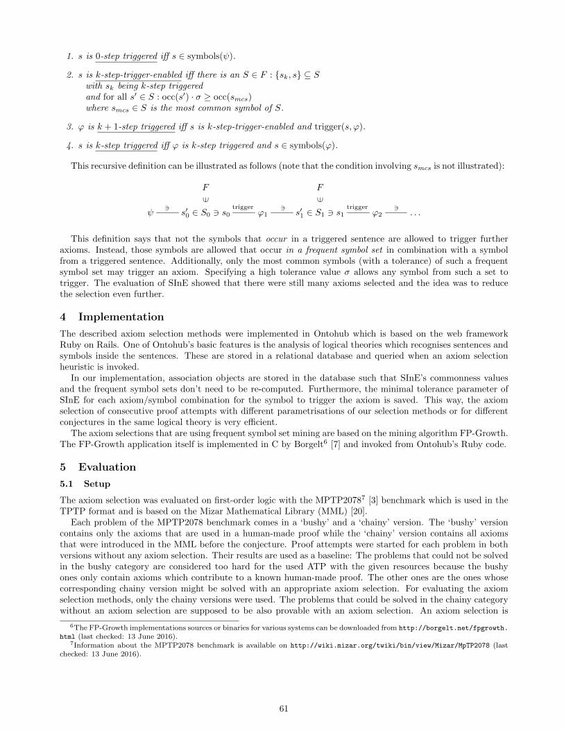
1. s is 0-step triggered iff s ∈ symbols(ψ).

2. s is k-step-trigger-enabled iff there is an S ∈ F : {sk, s} ⊆ Swith sk being k-step triggeredand for all s′ ∈ S : occ(s′) · σ ≥ occ(smcs)where smcs ∈ S is the most common symbol of S.

3. ϕ is k + 1-step triggered iff s is k-step-trigger-enabled and trigger(s, ϕ).

4. s is k-step triggered iff ϕ is k-step triggered and s ∈ symbols(ϕ).

This recursive definition can be illustrated as follows (note that the condition involving smcs is not illustrated):

F F

∈ ∈

ψ3

s′0 ∈ S0 3 s0trigger

ϕ13

s′1 ∈ S1 3 s1trigger

ϕ23

. . .

This definition says that not the symbols that occur in a triggered sentence are allowed to trigger furtheraxioms. Instead, those symbols are allowed that occur in a frequent symbol set in combination with a symbolfrom a triggered sentence. Additionally, only the most common symbols (with a tolerance) of such a frequentsymbol set may trigger an axiom. Specifying a high tolerance value σ allows any symbol from such a set totrigger. The evaluation of SInE showed that there were still many axioms selected and the idea was to reducethe selection even further.

4 Implementation

The described axiom selection methods were implemented in Ontohub which is based on the web frameworkRuby on Rails. One of Ontohub’s basic features is the analysis of logical theories which recognises sentences andsymbols inside the sentences. These are stored in a relational database and queried when an axiom selectionheuristic is invoked.

In our implementation, association objects are stored in the database such that SInE’s commonness valuesand the frequent symbol sets don’t need to be re-computed. Furthermore, the minimal tolerance parameter ofSInE for each axiom/symbol combination for the symbol to trigger the axiom is saved. This way, the axiomselection of consecutive proof attempts with different parametrisations of our selection methods or for differentconjectures in the same logical theory is very efficient.

The axiom selections that are using frequent symbol set mining are based on the mining algorithm FP-Growth.The FP-Growth application itself is implemented in C by Borgelt6 [7] and invoked from Ontohub’s Ruby code.

5 Evaluation

5.1 Setup

The axiom selection was evaluated on first-order logic with the MPTP20787 [3] benchmark which is used in theTPTP format and is based on the Mizar Mathematical Library (MML) [20].

Each problem of the MPTP2078 benchmark comes in a ‘bushy’ and a ‘chainy’ version. The ‘bushy’ versioncontains only the axioms that are used in a human-made proof while the ‘chainy’ version contains all axiomsthat were introduced in the MML before the conjecture. Proof attempts were started for each problem in bothversions without any axiom selection. Their results are used as a baseline: The problems that could not be solvedin the bushy category are considered too hard for the used ATP with the given resources because the bushyones only contain axioms which contribute to a known human-made proof. The other ones are the ones whosecorresponding chainy version might be solved with an appropriate axiom selection. For evaluating the axiomselection methods, only the chainy versions were used. The problems that could be solved in the chainy categorywithout an axiom selection are supposed to be also provable with an axiom selection. An axiom selection is

6The FP-Growth implementations sources or binaries for various systems can be downloaded from http://borgelt.net/fpgrowth.

html (last checked: 13 June 2016).7Information about the MPTP2078 benchmark is available on http://wiki.mizar.org/twiki/bin/view/Mizar/MpTP2078 (last

checked: 13 June 2016).

61

parameter SInE

SInE withFrequent Symbol

Set Mining

Simple Axiom Selectionusing Frequent Item Set

Mining

generality threshold g 0 0 -

depth limit d 5,∞ ∞ ∞tolerance value t 1.0, 1.2, 1.5, 2.0 1.0, 2.0 -

symbol set tolerance σ - 1.0, 2.0 -

min. absolute support smin - 1, 2 1, 2

short axiom tolerance t - - 0, 2

minimal symbol set size n - - 2

Table 1: Parameters used in the evaluation for each axiom selection method

considered not effective if fewer conjectures can be proven using it than without using it in the chainy category.It is possible that a selection hides axioms that are relevant for a proof and, hence, leads to no conclusion.However, a well performing selection should enable proving more conjectures by selecting all the relevant axiomsand hiding only irrelevant ones.

The experiments were conducted on an instance of Ontohub specifically set up for this work. This instanceruns on a machine with two Intel R© Xeon R© E5-2667 v2 processors with HyperThreading (resulting in 32 logicalprocessor cores) typically clocked at 3.3 GHz along with 256 GB of RAM.

For analysis and proving, 30 Hets instances were used in parallel. This puts heavy load on 30 of the cores.The asynchronous (to the web interface) processing of Hets responses is done by another 30 Ruby processes.Their workload alternates with that of the Hets processes, such that no additional cores are used extensively atthe same time. The web user interface’s workload is very low. During the evaluation, it is only called by Hetsto fetch the theory files and it does not put heavy use to another core. In total 30 cores were used completelyand one additional core was used with little load. This leaves one spare processor core for other tasks. Duringthe experiments, processor utilisation of around 70% was observed.

For the benchmark, SPASS v3.7 and the E Theorem Prover 1.8 were used. These are among the best-ratedfirst-order provers. Since E features an own implementation of SInE, this was not activated by only using theparameters -xAuto -tAuto among (soft) CPU time and memory limiting as well as input and output parameters.

The parameters for the axiom selections are shown in Table 1. Proof attempts were made with each combi-nation of these parameters. Each of the provers was given a timeout of 10 seconds.

During the run with the first SInE with Frequent Symbol Set Mining configuration, a very slow runtimebehaviour was observed for some examples. The selection for these examples was cancelled after about eighthours of selection runtime. As a consequence, a timeout for the axiom selection was implemented: If the axiomselection itself took longer than two minutes, the proof attempt was cancelled. The choice of two minutesis arbitrary. The selection timeout must be chosen considerably large to make sure that much CPU time isconsumed because it was measured using wall clock time. The controlled environment ensured that no otherCPU-hungry processes were running other than the axiom selection and proving (which are limited to less thanone process per core). Hence, it is unlikely that other processes used much CPU time that should have beengiven to the selection for a perfect timing evaluation (as it would have happened by measuring CPU time insteadof wall clock time). The selection timeout has to be much longer than the chosen proving timeout, though,because we want to analyse the selection run time as well. An axiom selection that consequently takes this muchlonger than proving a conjecture is not an acceptable method because the goal is not only to enable proofs butalso shorten the overall proving time which includes the axiom selection.

5.2 Results

In the MPTP2078 benchmark, only 2044 problems are non-trivial. The other 34 conjectures are equal to anaxiom and could be proved by Hets during static analysis using reflexivity of an entailment relation withoutinvoking an external prover. Only the 2044 non-trivial problems were used for the axiom selection methodevaluation.

The first figures in this section show stacked column charts of the performance: Figure 1 shows how manyproblems could be solved using SInE. The same goes for Figure 2 using SInE with Frequent Symbol Set Mining.Finally, Figure 3 shows the performance of the Simple Axiom Selection using Frequent Item Set Mining.

62

Top-rated first-order provers return a status of the proof attempt telling the result in a single word. Thesestatuses are defined in the SZS ontology [22]. The most common statuses used by provers are

(i) THM (Theorem): All models of the axioms are models of the conjecture.

(ii) CSA (CounterSatisfiable): Some models of the axioms are models of the conjecture’s negation.

(iii) TMO (Timeout): The prover exceeded the time limit.

Of these statuses, ‘THM’ and ‘CSA’ indicate a successful prover run, while ‘TMO’ shows that the prover did notfinish successfully. There are more such values indicating failures which are actually used by software, but ATPonly use the two values ‘THM’ and ‘CSA’ in case of success. We extended this ontology8 by a status specificallyfor proving with reduced axiom sets:

(iv) CSAS (CounterSatisfiableWithSubset): Some models of the selected axioms are models of the conjecture’snegation.

If a refutation of the conjecture is found using a strict subset of the axioms (which means that the prover returnswith ‘CSA’), we do not know whether the conjecture is really false or we have excluded an axiom that is crucial toa potentially existing proof. If the prover returns with ‘THM’, we know by monotonicity of entailment relationsthat the found proof is also a proof with the full axiom set.

When a prover returns with a proof (marked in the diagrams as ‘THM’) or a refutation (marked as ‘CSA’), aproblem is considered solved. When it returns with a refutation while only a true subset of the axioms was used(marked as ‘CSAS’), or with a proving timeout (marked as ‘TMO (Prover)’) or when the axiom selection takesmore than two minutes (marked as ‘TMO (Selection)’), the problem is considered still unsolved.

Num

ber o

f Pro

blem

s

0

500

1000

1500

2000

2500

Axiom Selection Parameters (t, d)

Bush

y

(1.0

, )

(1.0

, 5)

(1.2

, )

(1.2

, 5)

(1.5

, )

(1.5

, 5)

(2.0

, )

(2.0

, 5)

Chai

ny

THM CSA CSASTMO (Prover) TMO (Selection)

(a) E Theorem Prover

Num

ber o

f Pro

blem

s

0

500

1000

1500

2000

2500

Axiom Selection Parameters (t, d)

Bush

y

(1.0

, )

(1.0

, 5)

(1.2

, )

(1.2

, 5)

(1.5

, )

(1.5

, 5)

(2.0

, )

(2.0

, 5)

Chai

ny

THM CSA CSASTMO (Prover) TMO (Selection)

(b) SPASS

Figure 1: Performance of the provers in MPTP2078 using SInE

Figure 4 shows the average runtime in milliseconds of each axiom selection method over all parametrisations.It contains two values for each method. The first one is the average over all selections that did not reach thetwo-minute timeout. The second one is the average runtime of the selection, regardless whether or not thetimeout was reached. This, of course, counts every selection that was cancelled as two minutes.

Figure 5 shows how many axioms were selected on average using SInE. Both versions of the MPTP2078 withouta selection are displayed for reference. Due to a high amount of timeouts in the other two selection methods,they are not included in these statistics. The distortion caused by leaving out selections that encountered atimeout would be too high.

8Our modified SZS ontology can be found on http://ontohub.org/meta/proof_statuses.

63

Num

ber o

f Pro

blem

s

0

500

1000

1500

2000

2500

, smin, t)Axiom Selection Parameters (

Bush

y

(1.0

, 1, 1

.0)

(1.0

, 1, 2

.0)

(1.0

, 2, 1

.0)

(1.0

, 2, 2

.0)

(2.0

, 1, 1

.0)

(2.0

, 1, 2

.0)

(2.0

, 2, 1

.0)

(2.0

, 2, 2

.0)

Chai

ny

THM CSA CSASTMO (Prover) TMO (Selection)

(a) E Theorem Prover

, smin, t)Axiom Selection Parameters (

Num

ber o

f Pro

blem

s

0

500

1000

1500

2000

2500

Bush

y

(1.0

, 1, 1

.0)

(1.0

, 1, 2

.0)

(1.0

, 2, 1

.0)

(1.0

, 2, 2

.0)

(2.0

, 1, 1

.0)

(2.0

, 1, 2

.0)

(2.0

, 2, 1

.0)

(2.0

, 2, 2

.0)

Chai

ny

THM CSA CSASTMO (Prover) TMO (Selection)

(b) SPASS

Figure 2: Performance of the provers in MPTP2078 using SInE with Frequent Symbol Set Mining

Benchmark Size.

To interpret the results properly, we need to know the size of the benchmarks. For implementation reasons,there is no very easy way to count the symbols including duplicates. So, only the distinct symbols are taken intoaccount. This is regarded as a sufficient approximation for interpreting the results.

The MPTP2078 benchmark in the bushy version has between 2 and 232 axioms per problem. Its average is31.5 axioms with a standard deviation of 23.4. It has between 2 and 93 distinct symbols per problem with anaverage of 18.8 and a standard deviation of 12.1. Counting the distinct symbols per axiom, there are between 0and 26 symbols, 2.9 on average with a standard deviation of 2.7.

The chainy version of the MPTP2078 has between 10 and 4563 axioms per problem. The average axiom countis 1876.4 with a standard deviation of 1288.6. The number of distinct symbols per problem ranges from 5 to 784with an average of 266.7 and a standard deviation of 229.2. In the axioms, there are between 0 and 26 distinctsymbols, 4.9 on average with a standard deviation of 3.1.

5.3 Discussion

SInE.

Inspecting Figure 1, one can see that the E Theorem Prover improves by about 50% for most of the parametri-sations of SInE (45% on average) compared to the chainy versions without any selection. SPASS also performsmuch better with a selection than without one: Its manages to solve 64% more problems on average across theSInE parametrisations. As a side note, the E Theorem Prover performs better than SPASS, even when com-paring the E Theorem Prover without preselecting axioms against the best result with the selection for SPASS.Considering all SInE parametrisations, 769 problems could be solved, 330 of them could not be solved withoutan axiom selection. Without axiom selection, 444 problems could be solved.

For both provers, the number of ‘CSA’ and ‘CSAS’ results is negligible. For the largest tolerance value withouta depth limit, meaning (t, d) = (2.0,∞), the axiom selection takes more than two minutes for 294 examples.These examples have 2165.5 axioms on average with a standard deviation of 1680.1, ranging from 51 to 4563 and332.5 distinct symbols on average with a standard deviation of 298.7, ranging from 12 to 784. This means thatnot only the largest problems take long during axiom selection but also some of the small problems. Having atimeout on some of the small problems may be a result of a high CPU load caused by other tasks performed onthe hardware. It is imaginable that the timeout at the larger problems is due to the problem size, though.

64

Num

ber o

f Pro

blem

s

0

500

1000

1500

2000

2500

Axiom Selection Parameters (smin, t)

Bush

y

(1, 0

)

(1, 2

)

(2, 0

)

(2, 2

)

Chai

ny

THM CSA CSASTMO (Prover) TMO (Selection)

(a) E Theorem Prover

Axiom Selection Parameters (smin, t)

Num

ber o

f Pro

blem

s

0

500

1000

1500

2000

2500

Bush

y

(1, 0

)

(1, 2

)

(2, 0

)

(2, 2

)

Chai

ny

THM CSA CSASTMO (Prover) TMO (Selection)

(b) SPASS

Figure 3: Performance of the provers in MPTP2078 with the Simple Axiom Selection using Frequent Item SetMining

SInE with Frequent Symbol Set Mining.

Figure 2 clearly shows that there is no proving performance gain by SInE with Frequent Symbol Set Mining.Not only do both provers perform maximally as well as without the axiom selection but also the selection itselfis cancelled frequently due to timeouts. The number of ‘CSAS’ results increases for some parametrisations,but regarding there is such a high amount of selection timeouts, this can be ignored. In total, 475 MPTP2078problems could be solved using SInE with Frequent Symbol Set Mining, only 35 of which were not solved withoutan axiom selection.

Simple Axiom Selection using Frequent Item Set Mining.

Figure 3 shows that the timeout of the axiom selection is dominating the results. This means that for most ofthe problems, two minutes of selection time are not enough. Only 239 MPTP2078 problems could be solved intotal with this method, 9 of which could not be solved without a preselection in the chainy versions.

Selection Runtime.

Figure 4 shows the average runtime over all parametrisations of the presented selection methods. When onlyconsidering the problems that did not reach a timeout (red/left columns), SInE is the slowest method with anaverage runtime of 18.6 seconds per problem. This is not a fair comparison though, because the other two methodsoften reached the two-minute timeout while SInE did not. When counting two minutes for every timeout-reachedselection (which actually passed during the selection), SInE achieves the best result (yellow/right columns). Twominutes are the smallest value that can be used without distorting the data too much. The distortion caused bycounting two minutes is in favour of the axiom selection methods using frequent item set mining which are slowernevertheless. A runtime of several hours for a single problem was observed with SInE with Frequent Symbol SetMining, before a timeout was implemented. This time was mainly consumed by the external frequent item setmining process. The same behaviour is suspected for the Simple Axiom Selection using Frequent Item Set Mining.Since the MPTP2078 comprises large theories, these two slower methods are again considered unsuitable.

Number of Selected Axioms.

Figure 5 shows the average number of selected axioms using SInE. When the depth limit is set to 5, considerablyless axioms get selected than without a limitation in MPTP2078. Also, the difference between infinite depth

65

sele

ctio

n ru

ntim

e [m

s]

0100002000030000400005000060000700008000090000

100000110000

SInE SInE with FSSM Simple AS with FSSM

101858

3140219721

38001363018592

average of unexpired selections average of all selections

Figure 4: Runtime of axiom selection methods

Num

ber o

f sel

ecte

d Ax

iom

s

0

500

1000

1500

2000

Bush

y

(1.0

, )

(1.0

, 5)

(1.2

, )

(1.2

, 5)

(1.5

, )

(1.5

, 5)

(2.0

, )

(2.0

, 5)

Chai

ny

Figure 5: Average number of selected ax-ioms by SInE

limit and a limit of 5 increases with a growing tolerance value. As expected, the number of selected axiomshighly increases with a growing tolerance value.

Conclusion.

Considering the evaluation results, of the three selection methods, SInE clearly is the only usable method forlarge theories. The methods based on frequent symbol set mining take too much time for large problems andsometimes even for small problems. Even if the selection itself finishes quickly, the selected axioms do not enableproving considerably more conjectures. SInE on the other hand, allows to prove significantly more conjectures.For this reason, only SInE will be kept in Ontohub.

6 Related Work

Axiom selection was actively researched in the recent years. A simple algorithm called RedAx [24] was de-veloped to provide evidence for the effectiveness of preselected axioms when proving. SRASS [25] is a moresophisticated semantically operating algorithm to find the right axioms for a proof. MePo [13] as part of Is-abelle/Sledgehammer [16, 18] which is adding axioms that share a feature with the conjecture or already addedaxioms in several iterations. In each iteration, a pass mark is increased which makes it harder for axioms tobe added to the selection. This method was followed by MaSh [11] to improve Isabelle/Sledgehammer’s axiomselection with machine learning methods that rank axioms by the amount and kind of features they share withthe conjecture and takes into account previous proofs in the same theory. Alama et al. [3] use learning in MOR,in particular kernel methods, to determine how similar sentences are to each other and uses these similarityvalues to find feature weights and to eventually rank the available axioms. SInE [10] is a heuristic that, similarlyto MePo, iteratively adds axioms to the selection that share symbols with the conjecture or already selectedaxioms. Instead of increasing a pass mark, it only selects axioms that contain symbols whose number of occur-rences in the overall theory meets certain requirements. This method proved very successful by executing fastand enabling about as many proofs as some learning methods.

Because of saving intermediate information in a database, our implementation of SInE is very efficient forconsecutive runs, although because of the implementation in Ruby and because of being bound to a relationaldatabase the first run performs slower than an implementation with native/compiled code such as it existsdirectly in Vampire or E. One notable feature is the prover-independent operability of the axiom selection. Thisimplementation is usable with any prover that interfaces with Hets.

7 Conclusions and Future Work

An implementation of axiom selection heuristics was presented: the already existing SInE and two methodsbased on frequent item set mining. These are implemented in the combination of the web application Ontohuband Hets and run independently of the selected prover, which is a first step towards an implementation of logic-independent axiom selections in Ontohub. Currently, this implementation is compatible to every Hets-interfaced

66

first-order prover. The evaluation of the selection methods showed once again the effectiveness of the SInEalgorithm but also revealed that frequent item set mining is not an appropriate tool for selecting axioms becauseof the slow computation of frequent item sets.

Future work in this field should extend the feature of independence such that the axiom selections operateindependently of the logic as well. A new evaluation could feature a comparison between SInE as it is implementedin provers to the SInE implementation of Ontohub, measuring the performance of consecutive axiom selectionsthat are applied to the same theory (with different conjectures) such that the commonness values can be read fromthe database. Also learning methods could be incorporated into the selection, e.g. learning the best parametersfor SInE or entirely learning-based methods similar to MaSh or MOR could be incorporated. This is verypromising in the context of Ontohub because of its repository structure which stores information on every logicaltheory including proof attempts – both successful and failed.

References

[1] Charu C. Aggarwal and Jiawei Han. Frequent Pattern Mining. Springer Publishing Company, Incorporated,2014.

[2] Rakesh Agrawal and Ramakrishnan Srikant. Fast Algorithms for Mining Association Rules. In Proc. 20thint. conf. very large data bases, VLDB, volume 1215, pages 487–499, 1994.

[3] Jesse Alama, Tom Heskes, Daniel Kuhlwein, Evgeni Tsivtsivadze, and Josef Urban. Premise Selection forMathematics by Corpus Analysis and Kernel Methods. Journal of Automated Reasoning, 52(2):191–213,2014.

[4] Egidio Astesiano, Michel Bidoit, Helene Kirchner, Bernd Krieg-Bruckner, Peter D Mosses, Donald Sannella,and Andrzej Tarlecki. CASL: The Common Algebraic Specification Language. Theoretical Computer Science,286(2):153–196, 2002.

[5] Peter Baumgartner, Alexander Fuchs, and Cesare Tinelli. Darwin: A Theorem Prover for the ModelEvolution Calculus. In Stephan Schulz, Geoff Sutcliffe, and Tanel Tammet, editors, IJCAR Workshop onEmpirically Successful First Order Reasoning (ESFOR (aka S4)), Electronic Notes in Theoretical ComputerScience, 2004.

[6] Sascha Bohme and Tobias Nipkow. Sledgehammer: Judgement Day. In Automated Reasoning, pages 107–121. Springer, 2010.

[7] Christian Borgelt. Frequent Pattern Mining. Lecture slides. URL http://www.borgelt.net/teach/fpm/

slides.html. last checked: 13 June 2016.

[8] Peter Haase, Holger Lewen, Rudi Studer, Duc Thanh Tran, Michael Erdmann, Mathieu dAquin, and EnricoMotta. The Neon Ontology Engineering Toolkit. WWW, 2008.

[9] Jiawei Han, Jian Pei, and Yiwen Yin. Mining Frequent Patterns Without Candidate Generation. In ACMSigmod Record, volume 29, pages 1–12. ACM, 2000.

[10] Krystof Hoder and Andrei Voronkov. Sine Qua Non for Large Theory Reasoning. In Automated Deduction- CADE-23 - 23rd International Conference on Automated Deduction, Wroclaw, Poland, July 31 - August5, 2011. Proceedings, pages 299–314, 2011.

[11] Daniel Kuhlwein, Jasmin Christian Blanchette, Cezary Kaliszyk, and Josef Urban. MaSh: Machine Learningfor Sledgehammer. In Interactive Theorem Proving, pages 35–50. Springer, 2013.

[12] Eugen Kuksa and Till Mossakowski. Ontohub — version control, linked data and theorem proving forontologies. In FOIS 2016. To appear.

[13] Jia Meng and Lawrence C Paulson. Lightweight Relevance Filtering for Machine-Generated ResolutionProblems. Journal of Applied Logic, 7(1):41–57, 2009.

[14] Till Mossakowski. Heterogeneous Specification and the Heterogeneous Tool Set. University of BremenGermany, 2005. Habilitation thesis.

67

[15] Till Mossakowski, Mihai Codescu, Fabian Neuhaus, and Oliver Kutz. The Distributed Ontology, Modeling,and Specification Language - DOL. In A. Koslow and A. Buchsbaum, editors, The Road to Universal Logic,volume II of Studies in Universal Logic. Springer, 2015.

[16] Tobias Nipkow, Lawrence C Paulson, and Markus Wenzel. Isabelle/HOL: A Proof Assistant for Higher-Order Logic, volume 2283. Springer Science & Business Media, 2002.

[17] Natalya F Noy, Nigam H Shah, Patricia L Whetzel, Benjamin Dai, Michael Dorf, Nicholas Griffith, ClementJonquet, Daniel L Rubin, Margaret-Anne Storey, Christopher G Chute, et al. BioPortal: Ontologies andIntegrated Data Resources at the Click of a Mouse. Nucleic acids research, page gkp440, 2009.

[18] Lawrence C Paulson and Jasmin Christian Blanchette. Three Years of Experience With Sledgehammer, aPractical Link Between Automatic and Interactive Theorem Provers. IWIL-2010, 2010.

[19] Alexandre Riazanov and Andrei Voronkov. The Design and Implementation of VAMPIRE. AI communica-tions, 15(2, 3):91–110, 2002.

[20] Piotr Rudnicki. An Overview of the Mizar Project. In Proceedings of the 1992 Workshop on Types forProofs and Programs, pages 311–330, 1992.

[21] Stephan Schulz. System Description: E 1.8. In Ken McMillan, Aart Middeldorp, and Andrei Voronkov,editors, Proc. of the 19th LPAR, Stellenbosch, volume 8312 of LNCS, pages 735–743. Springer, 2013.

[22] G. Sutcliffe. The SZS Ontologies for Automated Reasoning Software. In G. Sutcliffe, P. Rudnicki, R. Schmidt,B. Konev, and S. Schulz, editors, Proceedings of the LPAR Workshops: Knowledge Exchange: AutomatedProvers and Proof Assistants, and The 7th International Workshop on the Implementation of Logics, number418 in CEUR Workshop Proceedings, pages 38–49, 2008.

[23] Geoff Sutcliffe. The 4th ijcar automated theorem proving system competition–casc-j4. Ai Communications,22(1):59–72, 2009.

[24] Geoff Sutcliffe and Alexander Dvorsky. Proving Harder Theorems by Axiom Reduction. In FLAIRS Con-ference, pages 108–113, 2003.

[25] Geoff Sutcliffe and Yury Puzis. SRASS - A Semantic Relevance Axiom Selection System. In AutomatedDeduction–CADE-21, pages 295–310. Springer, 2007.

[26] Geoff Sutcliffe, Jurgen Zimmer, and Stephan Schulz. TSTP Data-Exchange Formats for Automated TheoremProving Tools. Distributed Constraint Problem Solving and Reasoning in Multi-Agent Systems, 112:201–215,2004.

[27] Linus Torvalds and Junio Hamano. Git: Fast Version Control System, 2010. http://git-scm.com lastchecked: 13 June 2016.

[28] Christoph Weidenbach, Dilyana Dimova, Arnaud Fietzke, Rohit Kumar, Martin Suda, and Patrick Wis-chnewski. SPASS Version 3.5. In Automated Deduction–CADE-22, pages 140–145. Springer, 2009.

[29] Mohammed Javeed Zaki, Srinivasan Parthasarathy, Mitsunori Ogihara, and Wei Li. New Algorithms forFast Discovery of Association Rules. In KDD, volume 97, pages 283–286, 1997.

[30] Jurgen Zimmer and Serge Autexier. The MathServe System for Semantic Web Reasoning Services. InAutomated Reasoning, pages 140–144. Springer, 2006.

68

On Checking Kripke Models for Modal Logic K

Jean-Marie Lagniez Daniel Le Berre Tiago de Lima Valentin Montmirail

CRIL, Univ. Artois and CNRS, F62300 Lens, France{lagniez,leberre,delima,montmirail}@cril.fr

Abstract

This article presents our work toward a rigorous experimental com-parison of state-of-the-art solvers for the resolution of the satisfiabilityof formulae in modal logic K. Our aim is to provide a pragmatic wayto verify the answers provided by those solvers. For this purpose, wepropose a certificate format and a checker to validate Kripke modelsfor modal logic K. We present some experimental results using efficientsolvers modified to incorporate this verification step. We have beenable to validate at least one certificate for 67 percent of the satisfi-able problems, which provides a set of benchmark with independentlychecked solution which can be used to validate new solvers. We discussthe limits of our approach in the last part of this article.

1 IntroductionThe practical evaluation of running systems played a key role in the success of SAT solvers for classical proposi-tional logic [2, 18, 30]. When the latter became efficient enough to solve “real problems”, even more improvementswere observed, thanks to the huge interest on that new technology. We believe that such success can be repeatedfor many other systems. In this paper, we are interested in making it happen for satisfiability in modal logic K.

There are however a few conditions for that. First, there is a need for a common input format. For SAT, suchformat was provided thanks to the Second Dimacs Challenge [5]. While both a CNF and a generic format wereproposed in 1993, only the CNF format is currently supported by SAT solvers. Second, it is important to checkthe answers produced by a solver. There are several reasons why a solver could return an incorrect answer. Itmay contain bugs on corner cases such as trivial answers, very large files, very deep formulae, etc. It might alsobe the case that the solver does not read properly the input.

In the early days of the development of SAT solvers, the only kind of answer that could be checked was SAT:a model was given to a third party tool which could independently check that the formula was indeed satisfiedby that model [30]. More recently [16], checking UNSAT answers became also possible in practice for manysolvers: during its computation, the system writes in a log file some basic steps of the solver. This log file is thenanalysed and the answer can be verified.

For more complex logics, it is not always possible to check the answers produced by the solvers: take QBFfor instance, i.e. propositional logic plus quantifiers on variables. QBF solvers answers can hardly be verified.One would need to gather policies instead of a single model. While much effort has been devoted to producecertificates for QBF, it is still an open challenge [24]. Our work is in line with the one being done for QBF. Weaim at verifying, when possible, the answers provided by solvers for the satisfiability of modal logic K formulae,and building a library of benchmarks with verified answers to foster the development of new solvers. Therefore,we are faced with two problems: producing a certificate on the solver side and checking it using an independenttool. In this paper, we address both problems and present some experimental results with verified answers.

Copyright c© by the paper’s authors. Copying permitted for private and academic purposes.In: P. Fontaine, S. Schulz, J. Urban (eds.): Proceedings of the 5th Workshop on Practical Aspects of Automated Reasoning

(PAAR 2016), Coimbra, Portugal, 02-07-2016, published at http://ceur-ws.org

69

p2

ω0

p1; p2

ω1

p1

ω2

r1 r1

Figure 1: A Kripke Model.

The remainder of the paper is organised as follows. Section 2 presents the basic modal logic K, its syntax andsemantics. Section 3 presents the algorithm used for the verification of the certificates. Section 4 presents theI/O formats we propose for the certificates. In Section 5 we present the settings of our experimental evaluationwhose results are presented and discussed in the subsequent section. The final section draws some conclusionsand provides some followup research directions.

2 Preliminaries: Modal Logic KDefinition 2.1. The language of Modal Logic K (or simply K) is the language of classical propositional logicextended with 2 unary operators: � and ♦.

A formula of the form �ϕ (box phi) means ϕ is necessarily true. A formula of the form ♦ϕ (diamond phi)means ϕ is possibly true.

Definition 2.2 (Modal Depth). The modal depth of a formula ϕ in the language K, noted md(ϕ), is defined by(where ⊕ ∈ {∧,∨,→,↔}):

md(p) = md(>) = md(⊥) = 0md(¬ϕ) = md(ϕ)

md(ϕ⊕ ψ) = max(md(ϕ),md(ψ))md(�ϕ) = md(♦ϕ) = 1 + md(ϕ)

For example, md(�(p1 ∨ ♦p2 ∨ ♦p3)) = 2. The language K is interpreted using Kripke semantics [20], whichuses Kripke models.

Definition 2.3 (Kripke Model). Let a non-empty countable set of propositional variables P be given. A Kripkemodel is a triplet M = 〈W,R, I〉, where: W is a non-empty set of possible worlds; R is a binary relation on W(called accessibility relation); and I is a function which associates, to each p ∈ P , the set of possible worlds fromW where p is true.

Example 2.1. Let M = 〈W,R, I〉, where: W = {ω0, ω1, ω2}, R = {(ω0, ω1), (ω1, ω2)}, I ={(p1, {ω1, ω2}), (p2, {ω0, ω1})}. A graphical representation of M is given in Figure 1.

Definition 2.4 (Pointed Kripke Model). A pointed Kripke model is a pair 〈M,ω0〉, where M is a Kripke modeland ω0 is a possible world in W .

In the rest of the paper, we will simply use “model” to denote a “pointed Kripke model”.

Definition 2.5 (Satisfaction Relation). The satisfaction relation � between formulae and models is recursivelydefined as follows (the semantics of the operators >, ⊥, ∨ , → and ↔ is defined as usual):

M,ω � p iff ω ∈ I(p)M,ω � ¬ϕ iff M,ω 2 ϕM,ω � ϕ ∧ ψ iff M,ω � ϕ and M,ω � ψ

M,ω � �ϕ iff for all v if (ω, v) ∈ R then M,v � ϕ

M,ω � ♦ϕ iff there exists v such that (ω, v) ∈ R and M, v � ϕ

Definition 2.6 (Satisfiability). A formula ϕ is satisfiable in K if and only if there exists a model 〈M,ω0〉 thatsatisfies ϕ.

Definition 2.7 (Validity). A formula ϕ is valid in K if and only if every model 〈M,ω0〉 satisfies ϕ.

70

Definition 2.8 (K-Satisfiability Problem). Let ϕ be a formula in the language K. The K-satisfiability problem(K-SAT) is the problem of answering YES or NO to the question “Is ϕ satisfiable?”.

As one might expect, software trying to solve this problem may try to find a model that satisfies the formulagiven as input. If such model is found, the software can answer YES (or SAT) and provides the model to justifyits answer. However, the size of the model may be exponential in the size of the input. Indeed, K-SAT isPSPACE-complete [14, 21]. In this paper, we are interested in the practical aspects of model verification i.e., toknow in practice how big are such models, and how many of them could be checked.

3 Checking satisfiable answersAs mentioned in the introduction, it is important to be able to verify the answers given by the K-SAT solversbeing evaluated. Ideally, when a K-SAT solver answers SAT, it should also provide a certificate, a model. Suchan answer could thus be independently verified to check that it satisfies the input formula.

The method used to verify certificates amounts to what is commonly called Model Checking [6]. Severalapproaches to modal logic model checking can be found in the literature [7, 10, 27]. However, to the best of ourknowledge, those existing checkers are designed for logics that are different from K (often Temporal Logic) andtherefore are not easily adaptable to the task of checking a modal logic K model.

The algorithm we use is based on Algorithm 1, with a reasonable effort in the implementation to make itefficient enough to check the certificates produced in our experimental evaluation in reasonable time (less than300s). The code is written in C++ and accessible online1.

Algorithm 1: check(ϕ,M ,ωi)Data: ϕ: a formula, M : a model, ωi : a worldResult: true if M,ωi � ϕ, false otherwise

1 begin2 if (ϕ = �ψ) then3 for each ωj successor of ωi do4 if (not check(ψ,M,ωj)) then5 return false

6 return true

7 if (ϕ = ♦ψ) then8 for each ωj successor of ωi do9 if (check(ψ,M,ωj)) then

10 return true

11 return false

12 if (ϕ = (ψ ∧ φ)) then13 return (check(ψ,M,ωi) ∧ check(φ,M, ωi))14 if (ϕ = (ψ ∨ φ)) then15 return (check(ψ,M,ωi) ∨ check(φ,M, ωi))16 if (ϕ = ¬ψ) then return (not check(ψ,M,ωi))17 if (ϕ = pj) then return (M [ωi] contains pj)

The recursive function check() is called with the model provided by the K-SAT solver. Its correctness is easilyverified, as it implements each clause of Definition 2.5. Nonetheless, we still had to optimise the procedure. Tosee why, assume the following input formula ϕ = ♦p1 ∧♦p2 ∧ · · · ∧♦pn. An efficient way to generate a model forthis formula is to start with a possible world ω0 and create a new accessible world ωi for each sub-formula ♦pi

of ϕ. This is indeed what some of the solvers we tested do.Unfortunately, the procedure in Algorithm 1 is very inefficient to check that a model generated in this way

indeed satisfies ϕ. This is because, for each conjunct ♦pi of ϕ, the procedure will check if each possible worldωi satisfies pi: first, it takes the first conjunct ♦p1 and successfully checks p1 against ω1; then, it takes ♦p2 and

1http://www.cril.univ-artois.fr/˜montmirail/mdk-verifier

71

checks p2 against ω1, and fails; it checks p2 against ω2 and succeed; and so on. In the i-th iteration, it checks pi

against i possible worlds before succeeding. It is clear that the model checking procedure takes much more timeto finish than the satisfiability procedure itself. Indeed, the naive algorithm could not verify (in a reasonabletime) the majority of the models proposed as solution.

To minimise this problem, we used a kind of caching. On the i-th iteration, the procedure does not check onlypi against ωi, but also all sub-formulae of ϕ, and then stores the results on ωi. When it comes back to ω0, itdoes not need to explore ωi again. On the iteration i+ 1, if necessary, it goes directly to the unexplored worlds,thus starting from ωi+1.

The second optimisation deals with formulae of the form ♦♦ . . .♦p1. Here, the satisfiability method will createa long chain of possible worlds. Instead of exploring them one by one, the optimised algorithm stores the lengthof those chains of “empty possible worlds”, and jumps directly to the last possible world when necessary.

4 Input and Output FormatsThere exists several different input formats for modal logic. Among them, we can cite ALC, used by *SAT [11].For example, the formula ((p→ ♦q) ∧�q) is written in ALC as (AND (IMP C0 (SOME R0 C1)) (ALL R0 C1)).This format is purely textual, functional, but uses quantifiers (SOME, ALL) to express modal operators, whichcan be confusing. Another (very similar) example is KRSS [25]. The same formula can be written in KRSS as(((not C0) or (some R0 C1)) and (all R0 C1))). This format, in addition, lacks symbols for implicationand equivalence. As a third example, we can cite LWB [17]. The same formula is written in LWB as begin (p1=> dia(p2)) & box(p2) end. Unfortunately, this format does not allow for the most natural future extensionof our approach, namely, the representation of multiple modalities (multiple agents).

4.1 The Input format InToHyLo

We decided to use InToHyLo as input format. It is used, for example, by the solvers InKreSAT [19] and Spartacus[13]. The formula ((p → ♦q) ∧ �q) is written in InToHyLo as ((p1 -> <r1>p2) & [r1]p2 ). We believe thatthis format is easy to read and it is also easily adaptable for multiple modalities.

Definition 4.1 (InToHyLo Language). The InToHyLo Language is defined by the following Backus-Naur Formgrammar, where identifiers (id) are numerical sequences.

〈file〉 ::= ‘begin’ 〈fml〉 ‘end’

〈fml〉 ::= ‘(’ 〈fml〉 ‘)’| ‘true’ | ‘false’ | ‘p’〈id〉 | ‘˜’ 〈fml〉| ‘<r’ 〈id〉 ‘>’ 〈fml〉 | ‘[r’ 〈id〉 ‘]’ 〈fml〉| 〈fml〉 ‘&’ 〈fml〉 | 〈fml〉 ‘|’ 〈fml〉| 〈fml〉 ‘->’ 〈fml〉 | 〈fml〉 ‘<->’ 〈fml〉

Unary operators have the highest precedence in InToHyLo. The precedence of the binary operators is thefollowing: &, |, ->, <->.

4.2 The Output Format Flat Kripke Model

In order to be able to check answers produced by the solvers, we also propose an output format to representKripke models. This should be seen as an exchange format between softwares, and not something written directlyby a human, in the spirit of the DIMACS CNF format [5].

Below, we have a representation of the model in Figure 1 in the proposed format.

2 3 1 2-1 2 01 2 01 -2 0r1 w0 w1r1 w1 w2

The first line contains exactly four integers separated by spaces. They provide respectivelythe number of propositional variables, the number of possible worlds, the number of relations(which will be useful in the future for multi-modal problems), and finally the number of edgesin the model. In the subsequent lines, each propositional variable is represented by a positiveinteger. For example, if there exists 3 propositional variables in the model, then they are named1, 2 and 3. The second line corresponds to the valuation of the first possible world (i.e., ω0).The third line corresponds to the valuation of the second possible world (ω1), and so on. Each ofthese lines follows the DIMACS format [5]: the integer i means that the propositional variablei is assigned to true in that world and −i means that the propositional variable i is assigned to

72

false in that world. There must be exactly one valuation line for each possible world in the model. Each of theselines must end with a 0. After that, the connections between worlds are provided. Each line has the format: rIwJ wK, where I, J and K are integers. The first one represents the I-th relation of the model, the second one isthe J-th world and the third one is the K-th world. Each one of these lines means that ωK is reachable from ωJ

in the accessibility relation number I. There must be exactly one such line for each edge of the model.

5 Evaluation settings5.1 Solvers

There are numerous solvers for modal logic K, developed in the last two decade. Some of the earlier solvershave the ability to output a model: SPASS [33] provides the branches open in every world or LWB [15] whichprovide an image representing a Kripke model. However, those solvers are no longer “state-of-the-art” in termsof runtime (see e.g. [29, 1] for a comparison with more recent solvers considered here). We decided to considerall but one of the solvers used in [19], which is, to the best of our knowledge, the most recent paper comparingmodal logic K solvers. FaCT++ [32] (v1.6.1), an established reasoner for the web ontology language OWL 2 DL,is missing in our experiments because it is a Tableau solver like Spartacus generally outperformed by Spartacusaccording to [13].

Note that our goal in this work was not to perform a comparison of all existing solvers because we needed tomodify those solvers ourselves, but to show that it is possible to check the answers of different solvers using anindependent tool. We hope it will encourage other authors to allow their solvers to be able to output the modelin our Flat Kripke Model format.

5.1.1 Km2SAT

Km2SAT [29] translates modal logic formulae into an equisatisfiable CNF formula which can be solved by anySAT solver. We used Minisat 2.2.0 [8] in our experiments. If the formula is unsatisfiable, then the originalformula is unsatisfiable. If the formula is satisfiable, the satisfying assignment found can be transformed intoa model. In such case, we only need to interpret the assignment and output it using our proposed format.Unfortunately, Km2SAT, by default, may modify the input formula before applying the translation into CNF.Such optimisation preserves the satisfiability of the formula, but prevents us, in some cases, to retrieve a modelfor the original input.

Km2SAT reads formulae in the LWB format. Thus, we had to modify the original solver to allow it to readformulae in InToHyLo format. Such modification is obviously a threat to its correctness. We did our best tomake sure that the modifications on the input format did not impact the solver itself. To that end, we ran thesolver on examples using the LWB format supported by Km2SAT. Then, we used the Fast Transformation Tool(ftt) embedded with the software Spartacus [13] to transform those LWB problems into InToHyLo problems andwe checked if the modified version of Km2SAT returned the exact same models. This was performed on the 240instances of TANCS-2000-modKSSS, on the 80 instances of TANCS-2000-modkLadn, and on the 259 instancesof LWB solved by the modified Km2SAT. In all cases we obtained the same result.

5.1.2 *SAT

*SAT [11] (v1.3) is a reasoner for the description logic ALC. *SAT implements a modal extension of the Davis-Putnam procedure. But, because *SAT features several decision procedures of classical modal logics, it canperfectly be used as a K modal logic solver.

First of all, *SAT reads the ALC format. So, we had to modify the input parser in order to make thissolver read InToHyLo files. Because this threatens its correctness, we used the Fast Transformation Tool totranslate InToHyLo formatted benchmarks into ALC and then ran the original version of *SAT on the translatedbenchmarks. In all cases we obtained the same result.

Second, the interpretation of the result of *SAT is more challenging than for Km2SAT. Indeed, *SAT usesthe SAT solver in an interleaved and incremental approach: the SAT solver is called many times, since it drivesthe verification of the tableau rules. As such, analyzing a single SAT answer does not allow in general to retrievea complete model. For that reason, many of the SAT answers provided by *SAT could not be verified.

*SAT uses the SAT solver SATO [34] as backend. It was designed in the late nineties when only “small” CNFwhere considered. The solver accepts by default CNF with up to 10K variables and no more than 256 literals perclause. SATO may report unexpected results if those limits are enforced. We increased the variables boundary

73

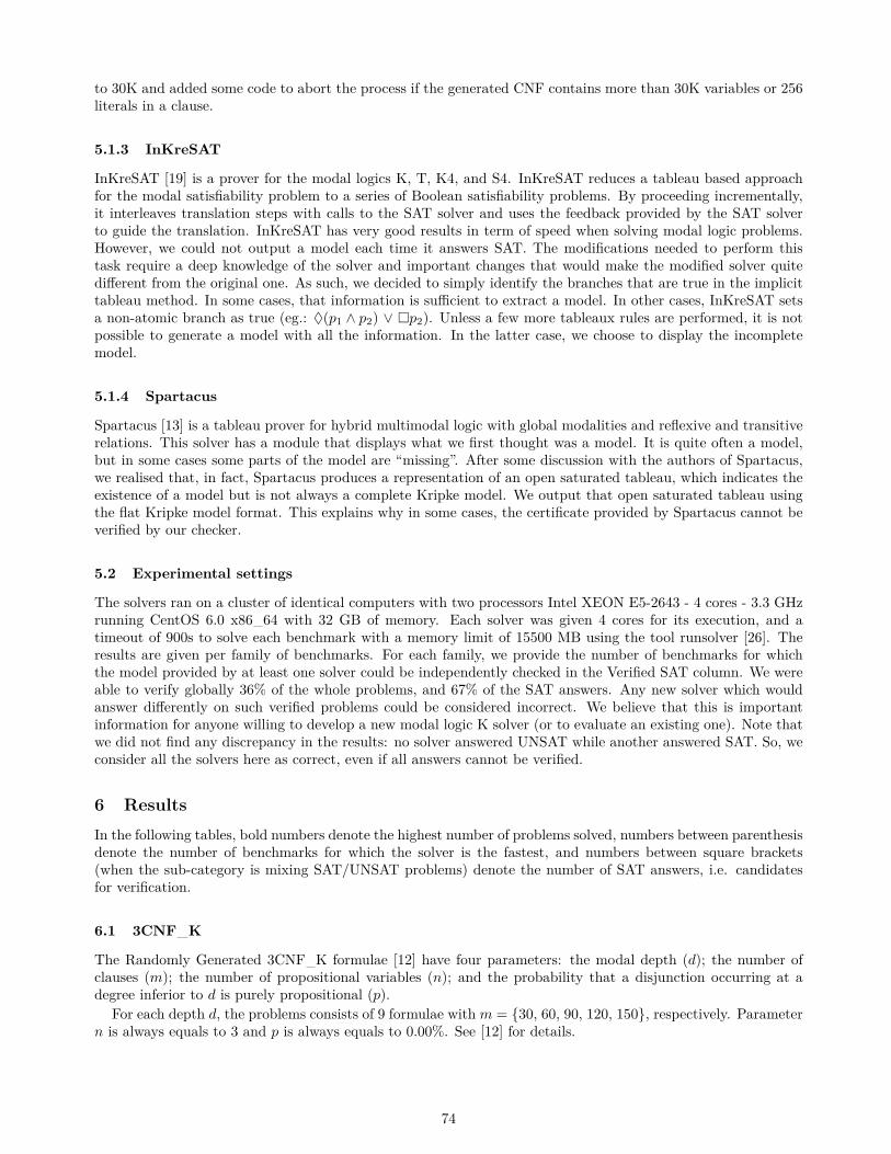
to 30K and added some code to abort the process if the generated CNF contains more than 30K variables or 256literals in a clause.

5.1.3 InKreSAT

InKreSAT [19] is a prover for the modal logics K, T, K4, and S4. InKreSAT reduces a tableau based approachfor the modal satisfiability problem to a series of Boolean satisfiability problems. By proceeding incrementally,it interleaves translation steps with calls to the SAT solver and uses the feedback provided by the SAT solverto guide the translation. InKreSAT has very good results in term of speed when solving modal logic problems.However, we could not output a model each time it answers SAT. The modifications needed to perform thistask require a deep knowledge of the solver and important changes that would make the modified solver quitedifferent from the original one. As such, we decided to simply identify the branches that are true in the implicittableau method. In some cases, that information is sufficient to extract a model. In other cases, InKreSAT setsa non-atomic branch as true (eg.: ♦(p1 ∧ p2) ∨ �p2). Unless a few more tableaux rules are performed, it is notpossible to generate a model with all the information. In the latter case, we choose to display the incompletemodel.

5.1.4 Spartacus

Spartacus [13] is a tableau prover for hybrid multimodal logic with global modalities and reflexive and transitiverelations. This solver has a module that displays what we first thought was a model. It is quite often a model,but in some cases some parts of the model are “missing”. After some discussion with the authors of Spartacus,we realised that, in fact, Spartacus produces a representation of an open saturated tableau, which indicates theexistence of a model but is not always a complete Kripke model. We output that open saturated tableau usingthe flat Kripke model format. This explains why in some cases, the certificate provided by Spartacus cannot beverified by our checker.

5.2 Experimental settings

The solvers ran on a cluster of identical computers with two processors Intel XEON E5-2643 - 4 cores - 3.3 GHzrunning CentOS 6.0 x86 64 with 32 GB of memory. Each solver was given 4 cores for its execution, and atimeout of 900s to solve each benchmark with a memory limit of 15500 MB using the tool runsolver [26]. Theresults are given per family of benchmarks. For each family, we provide the number of benchmarks for whichthe model provided by at least one solver could be independently checked in the Verified SAT column. We wereable to verify globally 36% of the whole problems, and 67% of the SAT answers. Any new solver which wouldanswer differently on such verified problems could be considered incorrect. We believe that this is importantinformation for anyone willing to develop a new modal logic K solver (or to evaluate an existing one). Note thatwe did not find any discrepancy in the results: no solver answered UNSAT while another answered SAT. So, weconsider all the solvers here as correct, even if all answers cannot be verified.

6 ResultsIn the following tables, bold numbers denote the highest number of problems solved, numbers between parenthesisdenote the number of benchmarks for which the solver is the fastest, and numbers between square brackets(when the sub-category is mixing SAT/UNSAT problems) denote the number of SAT answers, i.e. candidatesfor verification.

6.1 3CNF K

The Randomly Generated 3CNF K formulae [12] have four parameters: the modal depth (d); the number ofclauses (m); the number of propositional variables (n); and the probability that a disjunction occurring at adegree inferior to d is purely propositional (p).

For each depth d, the problems consists of 9 formulae with m = {30, 60, 90, 120, 150}, respectively. Parametern is always equals to 3 and p is always equals to 0.00%. See [12] for details.

74

d # Km2SAT *SAT InKreSAT Spartacus Verified SAT2 45 45 33 45 42 26 / 45 (57.78%)4 45 9/MO 20 12 45 45 / 45 (100.0%)6 45 0/MO 7 8 45 45 / 45 (100.0%)total 135 54 (0) 60 (2) 65 (13) 132 (120) 116 / 135 (85.92%)

Table 1: 3CNF K Results (d = modal depth)

All the problems are satisfiable, and all of them have been solved by at least one solver. Unfortunately, sincewe are not able to provide a certificate for all solvers, we were able to verify only the benchmarks for modal depthgreater than 2, which amounts to 85.92% of the problems. One may wonder why Spartacus solves problems whenthe modal depth is increasing, but does not perform as well as InKreSAT and Km2SAT when the modal depthis equal to 2. Basically, Spartacus did not manage to solve 3 instances with parameters m=150 and d=2. Thoseproblems with many clauses and a small modal depth are closer to a SAT problem than a modal-SAT problemfor which Spartacus is designed. This is also why InKreSAT and Km2SAT (which are SAT-based) performed sowell. On the smaller modal depth, only half of the answers are verified despite several solvers being able to decidethe satisfiability of the benchmarks. This is the consequence of Spartacus being the only provider of verifiedanswers on the whole set of benchmarks and that the saturated open tableau it generates is not a full Kripkemodel on small modal depth. *SAT did not perform as good as the other SAT based systems mainly becauseit calls more often its SAT solver. For instance, for the problem “c090v03p00d02s02”, *SAT called 30,179,676times its SAT solver while InKreSAT called Minisat 15 times and Km2SAT called Minisat only once. Note thatwe also experimented *SAT with Minisat: it does not help. The issue is really the number of SAT calls, not thesolver. The models returned by *SAT are surprisingly very small in number of worlds (compared to the othersolvers), but we cannot verify them because we do not have all the information needed to assign a truth valueto a given variable in a given world.

6.2 Randomly Generated modalized MQBF formulae

n,a # Km2SAT *SAT InKreSAT Spartacus Verified SAT4,4 40 MO 40 [18] 40 [18] 40 [18] 11 / 18 (61.11%)4,6 40 MO 40 [20] 39 [19] 40 [20] 9 / 20 (45.00%)8,4 40 MO 40 [31] 29 [22] 37 [28] 6 / 31 (19.35%)8,6 40 MO 31 [30] 16 [16] 34 [31] 0 / 33 (00.00%)16,4 40 MO 26 [25] 17 [16] 29 [28] 0 / 28 (00.00%)16,6 40 MO 25 [25] 16 [16] 29 [29] 0 / 29 (00.00%)total 240 MO 202 (41) 157 (1) 209 (173) 26 / 159 (16.35%)

Table 2: qbfMS

Randomly generated modalized MQBF formulae [22] are randomly generated QBF formulae translated to modallogic K. QBF with m clauses, alternation depth equal to a (the number of times that we changed the quantifierin the formula), with at most n variables per alternation. For each clause 4 different variables are randomlygenerated and each is negated with probability 0.5. The first and the third variables are existentially quantified,whereas the second and the fourth variables are universally quantified. A translation close to Schmidt-Schauß andSmolka’s reduction of QBF validity into ALC satisfiability [28] is used. The different values of the parameters forthis category of benchmarks are as follows: m ∈ {10, 20, 30, 40, 50} denotes the number of clauses; n ∈ {4, 8, 16}denotes the number of variables; a ∈ {4, 6} denotes the alternation depth. For each triplet (a, n,m) we have8 problems, so the whole family is composed of 240 problems. As already explained in the beginning of thissection, there is a possibility for a solver to do a memory-out. This is what happened to Km2SAT in the wholecategory. Contrariwise to the previous benchmark families, very few satisfiable benchmarks from qbfMS couldbe verified. Those formulae contain basically 1 variable, a lot of operators (modal and Boolean) and a very bigmodal depth. The issue with such “toy-problems” is that it is very difficult to verify a model for it. For thispurpose, we put a time-out on our checker of 300s. If we did not manage to verify the solution, we consider theSAT answers as unchecked. It happened only in this category, 103 times for Spartacus and 38 times for *SAT.

75

6.3 TANCS-2000 benchmarks for K Results

(a) Runtime distribution on modKLadn (b) Runtime distribution on modKSSS

Figure 2: Runtime distribution for TANCS 2000

The TANCS-2000 Unbounded Modal QBF [23] benchmarks are generated the same way as the previous onesexcept that a single relation in modal logic K is replaced by a sequence of back-forth-back relations, in a cleverway to avoid making most formulae unsatisfiable. These QBF formulae were originally converted to K using 3different techniques of increasing hardness. We ran only the sub-categories modKSSS (Schmidt-Schauss-Smolkatranslation, easy) and modKLadn (Ladner translation, medium) because the third one (Halpern translation, thehardest) was not available in Spartacus benchmark archive (nor in the results presented in [13]).

n,a # Km2SAT *SAT InKreSAT Spartacus Verified SAT4,4 40 40 [17] 40 [17] 40 [17] 40 [17] 17 / 17 (100%)4,6 40 40 [25] 40 [25] 40 [25] 40 [25] 23 / 25 (92.00%)8,4 40 40 [26] 40 [26] 40 [26] 40 [26] 26 / 26 (100%)8,6 40 14/MO [14] 38 [35] 37 [34] 40 [37] 18 / 37 (48.64%)16,4 40 8/MO [8] 33 [33] 36 [36] 40 [40] 21 / 40 (52.50%)16,6 40 8/MO [8] 32 [32] 38 [38] 40 [40] 15 / 40 (37.50%)total 240 150 (2) 223 (13) 231 (1) 240 (226) 120/ 185 (64.86%)4,4 40 40 [19] 40 [19] 40 [19] 40 [19] 19 / 19 (100%)4,6 40 40 [24] 11 [ 6] 38 [22] 39 [23] 24 / 24 (100%)total 80 80 (80) 51 (0) 78 (0) 79 (0) 43 / 43 (100%)

Table 3: Upper: modKSSS — Lower: modKLadn

Spartacus outperforms the other solvers on modKSSS benchmarks. The bigger the values of n and a, themore difficult it is to verify the model provided by the solver. It is interesting to note that on the modKLadnbenchmarks, Km2SAT performs much better than the other solvers, which can be seen in the runtime distributionof the solvers in Figure 2a. Here, the approach benefits from the advances on SAT solvers. Note that formodKSSS, Km2SAT simply cannot generate the CNF within our memory limit when it does not solve thosebenchmarks.

76

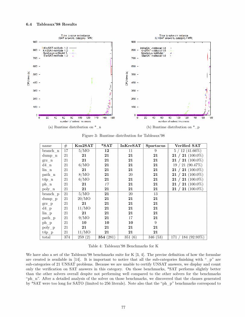
6.4 Tableaux’98 Results

(a) Runtime distribution on * n (b) Runtime distribution on * p

Figure 3: Runtime distribution for Tableaux’98

name # Km2SAT *SAT InKreSAT Spartacus Verified SATbranch n 17 5/MO 12 11 9 5 / 12 (41.66%)dump n 21 21 21 21 21 21 / 21 (100.0%)grz n 21 21 21 21 21 21 / 21 (100.0%)d4 n 21 6/MO 21 21 21 19 / 21 (90.47%)lin n 21 21 21 21 21 21 / 21 (100.0%)path n 21 8/MO 21 20 21 21 / 21 (100.0%)t4p n 21 6/MO 21 21 21 21 / 21 (100.0%)ph n 21 21 17 21 21 21 / 21 (100.0%)poly n 21 21 21 21 21 21 / 21 (100.0%)branch p 21 5/MO 21 20 13dump p 21 20/MO 21 21 21grz p 21 21 21 21 21d4 p 21 11/MO 21 21 21lin p 21 21 21 21 21path p 21 9/MO 21 17 21ph p 21 10 10 10 9poly p 21 21 21 21 21t4p p 21 11/MO 21 21 21total 374 259 (2) 354 (281) 351 (6) 346 (53) 171 / 184 (92.93%)

Table 4: Tableaux’98 Benchmarks for K

We have also a set of the Tableaux’98 benchmarks suite for K [3, 4]. The precise definition of how the formulaeare created is available in [14]. It is important to notice that all the sub-categories finishing with “ p” aresub-categories of 21 UNSAT problems. Because we are unable to certify UNSAT answers, we display and countonly the verification on SAT answers in this category. On those benchmarks, *SAT performs slightly betterthan the other solvers overall despite not performing well compared to the other solvers for the benchmarks“ph n”. After a detailed analysis of the solver on those benchmarks, we discovered that the clauses generatedby *SAT were too long for SATO (limited to 256 literals). Note also that the “ph p” benchmarks correspond to

77

(a) Spartacus with vs without model output (b) Km2SAT with vs without model output

Figure 4: overhead of our modifications

hard combinatorial UNSAT Pigeon-Hole problems [31], which explains why they are difficult for all solvers. Andfinally, all the “ n” are almost fully Verified SAT except “branch n”. Let take a closer look to the Kripke modelreturned for this category. The formula contains sub-formulae looking like (♦(x∧ y ∧ z)∧♦(x∧ y ∧¬z)) and theaccessibility relation between worlds must be a tree. Such formula requires 2 accessible worlds: one satisfying zand another satisfying ¬z. However Spartacus only provides one of them in its open tableau. The same kind ofincomplete models are returned by *SAT and InKreSAT. Only Km2SAT manages to provide complete Kripkemodels on this category, but unfortunately, Km2SAT solves only 5/17 problems, so we have only 5/17 verifiedsolutions.

6.5 On the importance of the SAT solvers

3 out of 4 solvers evaluated here are SAT-based. InKreSAT is tightly coupled with Minisat 2.2.0 [8], it is as suchvery difficult for us to use another backend SAT solver. As such, we used Minisat 2.2.0 with Km2SAT solver aswell. There are nowadays better SAT solvers (Glucose, Lingeling). Does it make any difference in our context?After some experimentation, we could only obtain a small speed gain by using Glucose instead of Minisat withKm2SAT. This gain is obtained in the category 3CNF where Glucose is much faster than Minisat. It is worthnoting that 754 out of the 766 times Km2SAT does not answer, it is because the CNF cannot be generated withthe available amount of memory, not because the CNF cannot be solved. We also tried to plug Minisat 2.2.0in *SAT instead of SATO. Indeed, *SAT is very efficient despite being coupled to a SAT solver created in thenineties. One would expect that it would get even better with a more recent SAT solver like Minisat or Glucose.Unfortunately, the developers of *SAT made the code deeply linked to SATO for efficiency reasons (they sharethe same data structures to store the CNF for instance). While it is possible to plug any recent SAT solver usinga file based approach, it is really inefficient compared to the tight integration with SATO. Note that the CNFproduced by *SAT are in many cases quite simple to solve, and do not require a much sophisticated SAT solver.One interesting research direction would be to design a *SAT like algorithm taking into account the currentincremental capabilities of SAT solvers.

6.6 Overhead of model production

We had to modify the solvers not only to produce the Kripke model but also to bookkeep information to beable to produce such model. As such, the performance of the solver may be affected by those modifications. Wecompared the runtime of the original solvers against the modified versions, to evaluate the overhead induced byour modifications. The difference in runtime may be important, as in Figure 4a, representing the runtime of

78

Spartacus in its original version (no-model) versus the version providing a model. All point above the diagonaldenote benchmarks for which the modified version of Spartacus takes longer than the original version. All thepoints at y=900 correspond to benchmarks that the original solver can solve (answer SAT) but for which themodified solver cannot produce the Kripke model within the timeout. The difference can be quite significantfor Spartacus because we rely on an existing debug ouput in the solver (i.e. non optimized) to generate thecertificate. There is certainly room for improvement here.

6.7 Verification of SAT answers per solver

We were able to check globally 67% of satisfiable problems for which at least one solver provided a Kripke model.However, while looking at Table 5, two solvers are the main providers of those verified answers.

#SAT #Verified Uniquely VerifiedKm2SAT 330 168 39/476

*SAT 584 6 0/476InKreSAT 573 26 0/476Spartacus 696 443 352/476

Global 708 476 391/476

Table 5: Statistics about the verification

Spartacus provided the most important number of certificates both because it is quite efficient and because itwas designed to provide an open tableau model for debugging purposes, which is often sufficient to build a Kripkemodel. Km2SAT provides the remaining certificates because we simply have to interpret the answer providedby the SAT solver. While such model is not always a model of the original formula but of a simplified one, inpractice it works in half of the cases.

6.8 Challenging models

The biggest Kripke model that we manage to verify was a model returned by Km2SAT on the instance modKSSS-C20-V8-D6.7. The Kripke model contained 10,618,391 worlds and 10,618,390 edges for 56 vars. It could beverified in 23,68s. Behind this Kripke model, Km2SAT generated a SAT formula with 108,700,724 variables and122,697,799 clauses. It took 273.620 seconds to generate this file of 3 GB plus the mapping file of 1 GB bytes.Then this SAT problem was solved in 87.049 seconds. Then, it took 291 seconds to parse the SAT solution andthe mapping to finally generate this Kripke model. The smallest Kripke model that we did not manage to verifyunder 300s was a model returned by *SAT on the instance modKSSS-K4-C10-V16-D4.4. The Kripke modelcontained 81 worlds and 2792 edges for 80 variables. This model is shown in Figure 5.

Figure 5: Unverified model from *SAT

79

7 Conclusion and perspectiveIn this paper, we studied the feasibility to verify in practice Kripke models returned by a selection of existingsolvers on a selection of existing benchmarks for modal logic K. For that purpose, we designed the Flat KripkeModel format to represent those models and built an independent model checker for modal logic K. We modifiedseveral solvers for modal logic K to provide such models and ran them on a wide range of existing benchmarks.We have been able to verify 67 percent of all the satisfiable benchmarks, which demonstrates that in practice,we can check the majority of SAT answers on current benchmarks. Our results also showed that it is a nonobvious task to modify existing solvers to output a Kripke model if the solver was not designed for that in thefirst place: by providing a specific textual format and a checker to the community, we would like to encouragesolver designers to provide the ability to produce models in that format. We plan to increase the number ofcheckable SAT answers by both improving the output of the models in efficient solvers such as Spartacus andKm2SAT, and improving the checker itself. A next logical step would be to study the feasibility to validateUNSAT answers, in the spirit of what is already done for SAT, based on the previous work on UNSAT proofs inthe modal logic K [9].

Acknowledgements

The authors thank Olivier Roussel for providing support for running the experiments. Part of this work wassupported by the French Ministry for Higher Education and Research and the Nord-Pas de Calais RegionalCouncil through the “Contrat de Plan Etat Region (CPER)” and by an EC FEDER grant.

References[1] C. Areces and M. de Rijke. Computational modal logic. 2003.

[2] A. Balint, A. Belov, M. Jarvisalo, and C. Sinz. Overview and analysis of the SAT Challenge 2012 solvercompetition. Artif. Intell., 223:120–155, 2015.

[3] P. Balsiger and A. Heuerding. Comparison of theorem provers for modal logics : introduction and summary.In Autom. Reasoning with Analytic Tableaux and Related Methods, pages 25–26. Springer, 1998.

[4] P. Balsiger, A. Heuerding, and S. Schwendimann. A Benchmark Method for the Propositional Modal LogicsK, KT, S4. J. Autom. Reasoning, 24(3):297–317, 2000.

[5] D. Challenge. Satisfiability: Suggested Format. DIMACS Challenge. DIMACS, 1993.

[6] E. M. Clarke, O. Grumberg, and D. Peled. Model checking. MIT press, 1999.

[7] L. A. Dennis, M. Fisher, N. Lincoln, A. Lisitsa, and S. M. Veres. Practical Verification of Decision-Makingin Agent-Based Autonomous Systems. CoRR, abs/1310.2431, 2013.

[8] N. Een and N. Sorensson. An Extensible SAT-solver. In Theory and Applications of Satisfiability Testing,6th International Conference, SAT 2003. Selected Revised Papers, pages 502–518, 2003.

[9] P. Enjalbert and L. F. del Cerro. Modal Resolution in Clausal Form. Theor. Comput. Sci., 65(1):1–33,1989.

[10] O. Gasquet, A. Herzig, B. Said, and F. Schwarzentruber. Kripke’s Worlds - An Introduction to Modal Logicsvia Tableaux. Studies in Universal Logic. Birkhauser, 2014.

[11] E. Giunchiglia and A. Tacchella. System description: *SAT: A platform for the development of modaldecision procedures. In Automated Deduction - CADE-17 Proceedings, pages 291–296, 2000.

[12] E. Giunchiglia, A. Tacchella, and F. Giunchiglia. SAT-Based Decision Procedures for Classical Modal Logics.J. Automated Reasoning, 28(2):143–171, 2002.

[13] D. Gotzmann, M. Kaminski, and G. Smolka. Spartacus: A Tableau Prover for Hybrid Logic. ENTCS,262:127–139, 2010.

80

[14] J. Y. Halpern and Y. Moses. A Guide to Completeness and Complexity for Modal Logics of Knowledge andBelief. Artificial Intelligence, 54(2):319–379, 1992.

[15] A. Heuerding, G. Jager, S. Schwendimann, and M. Seyfried. Propositional logics on the computer. InTheorem Proving with Analytic Tableaux and Related Methods, pages 310–323. Springer, 1995.

[16] M. Heule, W. A. H. Jr., and N. Wetzler. Trimming while checking clausal proofs. In FMCAD 2013., pages181–188, 2013.

[17] G. Jaeger, P. Balsiger, A. Heuerding, and S. Schwendiman. LWB 1.1 Manual. Unpublished, 1997.

[18] M. Jarvisalo, D. L. Berre, O. Roussel, and L. Simon. The International SAT Solver Competitions. AIMagazine, 33(1), 2012.

[19] M. Kaminski and T. Tebbi. InKreSAT: Modal Reasoning via Incremental Reduction to SAT. In AutomatedDeduction - CADE-24 Proceedings, pages 436–442, 2013.

[20] S. A. Kripke. Semantical analysis of modal logic i normal modal propositional calculi. Mathematical LogicQuarterly, 9(5-6):67–96, 1963.

[21] R. E. Ladner. The computational complexity of provability in systems of modal propositional logic. SIAMJournal of Computing, 1977.

[22] F. Massacci. Design and Results of the Tableaux-99 Non-classical (Modal) Systems Comparison. In Autom.Reasoning, International Conf., ’99 Proceedings, pages 14–18, 1999.

[23] F. Massacci and F. M. Donini. Design and Results of TANCS-2000 Non-classical (Modal) Systems Com-parison. In Autom. Reasoning., International Conf., 2000 Proceedings, pages 52–56, 2000.

[24] M. Narizzano, C. Peschiera, L. Pulina, and A. Tacchella. Evaluating and certifying QBFs: A comparison ofstate-of-the-art tools. AI Communications, 22(4):191–210, 2009.

[25] P. Patel-Schneider and B. Swartout. Description-logic knowledge representation system specification fromthe KRSS group of the ARPA knowledge sharing effort, 1993.

[26] O. Roussel. Controlling a solver execution with the runsolver tool system description. Journal on Satisfia-bility, Boolean Modeling and Computation, 7:139–144, 2011.

[27] A. Saffidine. Minimal proof search for modal logic K model checking. CoRR, abs/1207.1832, 2012.

[28] M. Schmidt-Schauß and G. Smolka. Attributive Concept Descriptions with Complements. Artificial Intel-ligence, 48(1):1–26, 1991.

[29] R. Sebastiani and M. Vescovi. Automated reasoning in modal and description logics via SAT encoding: thecase study of k(m)/alc-satisfiability. J. Artif. Intell. Res. (JAIR), 35:343–389, 2009.

[30] L. Simon, D. Berre, and E. A. Hirsch. The SAT2002 competition. Annals of Mathematics and ArtificialIntelligence, 43(1):307–342, 2004.

[31] W. A. Trybulec. Pigeon hole principle. JFM, 2(199):0, 1990.

[32] D. Tsarkov and I. Horrocks. FACT++ Description Logic Reasoner: System Description. In IJCAR 2006Proceedings, pages 292–297, 2006.

[33] C. Weidenbach, U. Brahm, T. Hillenbrand, E. Keen, C. Theobald, and D. Topic. Spass Version 2.0. In Aut.Deduction CADE18, pages 275–279. Springer, 2002.

[34] H. Zhang. SATO: An Efficient Propositional Prover. In Automated Deduction - CADE-14 Proceedings,pages 272–275, 1997.

81

Towards a Substitution Tree Based Index for

Higher-order Resolution Theorem Provers

Tomer Libal Alexander Steen

Inria SaclayPalaiseau, France

tomer.libal@inria.fr

Freie Universitat BerlinBerlin, Germany

a.steen@fu-berlin.de

Abstract

One of the reasons that forward search methods, like resolution, areefficient in practice is their ability to utilize many optimization tech-niques. One such technique is subsumption and one way of utilizingsubsumption efficiently is by indexing terms using substitution trees.In this paper we describe an attempt to extend such indexes for the useof higher-order resolution theorem provers. Our attempt tries to handletwo difficulties which arise when extending the indexes to higher-order.The first difficulty is the need for higher-order anti-unification. Thesecond difficulty is the closure of clauses under associativity and com-mutativity. We present some techniques which attempt to solve thesetwo problems.

1 Introduction

Term indexing is a popular technique for speeding up computations to a broad variety of tools in computationallogic, ranging from resolution based theorem provers [17] to interpreters of programming languages such asProlog. A key aspect for optimizing such tools is to use sophisticated methods for redundancy elimination. Onesuch method for clause-based indexes is subsumption. Forward subsumption allows to discard clauses which areless general than clauses already processed, whereas backward subsumption allows to remove stored clauses if amore general one is encountered. The idea behind both is that using more general clauses drastically reduces thesearch space while still being enough for completing certain tasks [9]. Due to the importance of subsumption inpractical applications, there is a variety of indexing techniques that support efficient subsumption queries. Werefer the reader to the survey about term indexing by Ramakrishnan et al. [16].

In a similar way to tools for first-order logic, higher-order logic tools can benefit also from term indexingfor efficient subsumption. Unfortunately, higher-order matching, which is a required technique for determiningsubsumption, is much more complex than its first-order counter part [21]. We only know of few approachesto higher-order term indexing: Theiß and Benzmuller designed a term index [22] for the LEO-II higher-orderresolution theorem prover [3]. However, their approach focuses on efficient low-level term (traversal) operationssuch as β-normalization and occur-checks. Additionally, term sharing is employed in order to reduce spaceconsumption and for allowing constant-time equality checks between α-equivalent terms.

The closest to our approach is the higher-order term indexing technique by Pientka [14]. Both approachesare based on substitution trees [6] and on propagating to the leaves those components of the indexed terms for

Copyright c© by the paper’s authors. Copying permitted for private and academic purposes.

In: P. Fontaine, S. Schulz, J. Urban (eds.): Proceedings of the 5th Workshop on Practical Aspects of Automated Reasoning(PAAR 2016), Coimbra, Portugal, 02-07-2016, published at http://ceur-ws.org

82

which there is no efficient unification algorithm. One difference is the assumed term representation: In order toefficiently manage more complex type systems, such as dependent types, Pientka has chosen to represent termsusing Contextual Modal Type Theory [12]. This technique allows for an elegant treatment of dependent typesbut requires a specially designed unification procedure [15]. Our use of the standard simple type theory [4] allowsus to use type-independent unification algorithms [2]. Another difference is the technique chosen for propagatingthe non-pattern content: While we use an efficient algorithm for computing the pattern generalization of twonon-pattern terms [2] (also made possible by our choice of term representation), Pientka’s technique is basedon a normalizing pre-processing step [15] which computes the non-pattern content as additional constraintsand might incur an additional cost. A somewhat less crucial difference is the treatment of associativity andcommutativity (AC). Since unification algorithms which incorporate this theory do not exist for higher-orderlogic, we deal with the problem by integrating the treatment of AC into the operations of the index. Pientka’sindex primary target are not terms in clausal form and therefore, this problem is not treated there. It should notbe too complex, though, to integrate the ideas presented in this paper in Pientka’s index in order to achieve thesame AC treatment. Obvious other differences include the state of the art of Pientka’s index, its implementationwithin the Twelf system [13], and the experimental results which are included and its rigorous representation.Our index is yet to be implemented and experimented with and we are still to provide fully rigorous presentation.Nevertheless, we believe that our approach might be more suitable for indexing higher-order terms in generalhigher-order theorem provers. This claim is, of course, to be justified by the implementation and experimentationof both indexing techniques within Leo-III [24].

In this paper we hence present a higher-order indexing technique for the theorem prover Leo-III which is alsobased on substitution trees. The differences just discussed and especially the treatment of non-pattern termsmight suggest that forward and backward subsumption operations can be efficiently handled by our approach.

The main difficulty which arises when trying to store clauses in an index is that the index must be closedunder the AC properties of clauses. In addition, when computing subsumed clauses, the number of literals inthe clause is not as important as the fact that each literal in the subsuming clauses must generalize a literal inthe subsumed one. As long as we only treat unit clauses, no special treatment is required and the techniquepresented in [7] can be safely extended to deal with higher-order terms. When dealing with multi-literal clauses,though, one has to compensate between optimizing the size of the index and optimizing the operations over theindex. As can be seen in [23], one cannot avoid an expensive backtracking search.

We suggest a different approach which is supposed to take advantage on searching the index in parallel. Inorder to achieve that, we plan to store each literal independently in the index and on subsumption calls, toretrieve and compare the literals in parallel. Due to the fact that Leo-III is based on a multi-agent architecture[20], we hope that such an approach would be efficient in practice.

Since we are using substitution trees, we are still faced with the problem of using the costly higher-orderunification and anti-unification procedures. In the presented work we somehow avoid this problem by using avariant of higher-order anti-unification [2] which computes pattern [11] substitutions. The use of this algorithmwill allow us to maintain a substitution tree all of whose inner nodes are pattern substitutions, on which unificationand anti-unification are efficient.

The definitions and properties of our index are still being investigated and some of them are not yet formallyproved. Nevertheless, we hope that the arguments and examples will convince the reader about the potential ofour approach for the indexing of arbitrary higher-order clauses and for the support of the forward and backwardsubsumption functions over this index.

In the next section we present the necessary definitions required for understanding this paper as well as thebasic ideas of substitution trees and higher-order anti-unification. Following this section is the main part of thepaper, in which we introduce our notion of higher-order substitution trees and define the insert, delete, retrieveand subsumption functions. We close our paper with a conclusion which also describes potential future work.

2 Preliminaries

In this section we present the logical language that is used throughout the paper. The language is a version ofChurch’s simple theory of types [4] with an η-conversion rule as presented in [1] and with implicit α-conversions.Unless stated otherwise, all terms are implicitly converted into β-normal and η-expanded form.

Let T0 be a set of basic types, then the set of types T is generated by T := T0 | T→ T. Let C be a signatureof function symbols and let V be a countably infinite set of variable symbols. In our definitions and examplesthe symbols u,w, x, y, z,W,X, Y, Z ∈ V, and f, g, h, k, a, b, c ∈ C are used. We sometimes use subscripts and

83

superscripts as well. The set Termα of terms of type α is generated by Termα := fα | xα | (λxβ .Termγ) |(Termβ→αTermβ) where f ∈ C, x ∈ V and α ∈ T (in the abstraction, α = β → γ). Applications throughout thepaper will be associated to the left. We will sometimes omit brackets when the meaning is clear. We will alsonormally omit typing information when it is not crucial for the correctness of the results. τ(tα) = α refers to thetype of a term. The set Term denotes the set of all terms. positions are defined as usual. We denote the subtermof t at position p by t|p. Bound and free variables are defined as usual. Given a term t, we denote by hd(t) itshead symbol.

Substitutions and their composition (◦) are defined as usual, namely (σ ◦ θ)(X) = θ(σ(X)). The domain andcodomain of a substitution σ are denoted by dom(σ) and codom(σ). The image of σ is the set of all variables incodom(σ). We denote by σ|W the substitution obtained from substitution σ by restricting its domain to variablesin W . We denote by σ[X 7→ t] the substitution obtained from σ by mapping X to t, where X might alreadyexist in the domain of σ. The join of two substitutions σ and θ is denoted σ • θ (cf. [7]). We extend theapplication of substitutions to terms in the usual way and denote it by postfix notation. Variable capture isavoided by implicitly renaming variables to fresh names upon binding. A substitution σ is more general thana substitution θ, denoted σ ≤ θ, if there is a substitution δ such that σ ◦ δ = θ. Similarly, a substitution σ isthe most specific generalization of substitutions τ and θ if σ ≤ τ , σ ≤ θ and there is no other substitution δfulfilling these properties such that δ > σ. A substitution σ matches a substitution τ if there is a substitution δsuch that δ ◦ τ = σ. A complete set of matchers between substitutions σ and τ is a set A of substitutions suchthat A contains all the matching substitutions between σ and τ . A substitution σ is a renaming substitution ifcodom(σ) ⊆ V and |codom(σ)| = |dom(σ)|. The predicate rename(σ) is true iff σ is a renaming substitution. Wedenote the inverse of a renaming substitution σ by inverse(σ).

2.1 Substitution Trees

This section describes substitution trees based on those defined in [6]. In order to optimize some functions ontrees, the definition in [6] uses normalized terms and substitutions. As we will see, we will insert the literals ofa clause independently into the index and therefore, if we normalize them as suggested in [6] the relationshipbetween the free variables among the different literals will be lost. The main differences, therefore, between ourpresentation and that in [6] is that we will avoid normalizing terms and substitutions and in addition, allowterms to be of arbitrary order.

Definition 1 (Substitution Trees). A substitution tree is defined inductively and is either the empty tree ε orthe tuple (σ,Π) where σ is a substitution and Π is a set of substitution trees such that

1. each node in the tree is either a leaf node (σ, ∅) or an inner node (σ,Π) with |Π| ≥ 2.

2. for every branch (σ1,Π1), . . . , (σn,Πn) in a non-empty tree we havedom(σi) ∩ (dom(σ1) ∪ . . . ∪ dom(σi−1)) = ∅ for all 0 < i ≤ n.

2.2 Higher-order Anti-unification

Anti-unification denotes the problem of finding a generalization t of two given terms t1 and t2, i.e. a term tsuch that there exist substitutions σ1, σ2 such that tσ1 = t1 and tσ2 = t2. A key algorithm for the procedureswhich are described in the remainder of this paper is the higher-order anti-unification algorithm of Baumgartneret al. [2]. This algorithm differs from most higher-order unification and anti-unification procedures not only bybeing applicable to arbitrary (simply typed) higher-order terms, but also by efficiently computing very specificgeneralizations.

By very specific generalization (in contrast to the most specific one) we here mean the most specific higher-order pattern which generalizes two arbitrary higher-order terms. This pattern, however, might not be the mostspecific generalization of these two higher-order terms. Higher-order patterns are restricted forms of higher-orderterms for which it is known that efficient unification algorithms exist [11].

Details about the higher-order pattern fragment or even the above anti-unification algorithm are not crucialfor understanding this paper and are therefore omitted. It is important to note that since only most specificpattern generalizations are found, the size of the index described in this paper is not optimal. We will explainthis point in more detail later.

The anti-unification algorithm of Baumgartner et al. is subsequently denoted by msg∗.

84

Definition 2 (Algorithm msg∗ [2]). The algorithm msg∗ takes two arbitrary higher-order terms t1 and t2 asinput and returns a higher-order pattern s and substitutions σ1 and σ2 such that

1. sσ1 = t1 and sσ2 = t2, and

2. there is no other higher-order pattern s′ fulfilling the above property such that there is a non-trivial substi-tution δ where sδ = s′.

Baumgartner et al. showed that the algorithm msg∗ computes a unique solution (up to renaming of freevariables) and takes cubic time [2]. In this paper we are interested in a variant of this algorithm which computessubstitutions, rather than terms and which is defined as follows:

Definition 3 (Most specific pattern generalizing substitution). Given substitutions θ1 and θ2, the substitutionσ is the most specific pattern generalizing substitution if there are substitutions τ1 and τ2 such that codom(σ)contains only higher-order patterns, σ ◦ τ1 = θ1, σ ◦ τ2 = θ2 and there is no substitution σ′ > σ fulfilling theseproperties.

An algorithm for computing the most specific pattern generalizing substitution, denoted msg, can be definedon top of msg∗.

Definition 4 (The algorithm msg). The algorithm msg takes two substitutions θ1, θ2 as input and returns a triple(σ, τ1, τ2) with σ, τ1, τ2 as in Def. 3. To that end, let dom(θ1)∪dom(θ2) = {x1, . . . , xn}. Let (f(s1, . . . , sn), τ1, τ2) =msg∗(f(θ1(x1), . . . , θ1(xn)), f(θ2(x1), . . . , θ2(xn))) where f is a new function symbol of arity n. Finally, setσ := {x1 7→ s1, . . . , xn 7→ sn}.

Claim 5. Let θ1, θ2 be two substitutions and let (σ, τ1, τ2) = msg(θ1, θ2). Then σ is a most specific patterngeneralizing substitution of θ1 and θ2. Also, σ is unique up to renaming of free variables.

The algorithm msg takes cubic time, hence can be used to efficiently build up a substitution tree index (cf.next section).

3 Substitution Trees for Higher-order Clauses

In this section we will describe some modifications to first-order substitution trees which will allow us to extendthem to higher-order terms.

The most obvious obstacle in extending the trees to higher-order terms is the fact that substitution trees de-pend on procedures for unification, anti-unification and matching. These procedures, while being both relativelyefficient and unitary in classical first-order logic [10], are highly complex in higher-order logics and do not possessunique solutions any more [8, 19].

Another obstacle is the fact that since we are targeting resolution theorem provers, the terms we are goingto store, retrieve, delete and check for subsumption are not mere syntactic terms but clauses with are closedunder AC. In the first-order case, one can use dedicated unification algorithms which, although not unitary anymore [5], are still feasible. In the higher-order case, due to the complex nature of even the syntactic unificationprocedure, one needs to find another approach.

Our solution to the first problem is to relax a core property of substitution trees and allow also non leastgeneral generalizations as substitutions in the nodes of the trees. Towards this end, we employ the anti-unificationalgorithm from section 2.2. The use of this algorithm will render our trees less optimal as nodes may now containmore general substitutions than necessary and therefore one child may be more general than another child of anode. On the other hand, the algorithm is only cubic in time complexity and is unitary.

Our approach to the second problem is to handle the AC properties of clauses not on the anti-unification ormatching level, but to encode their treatment into the retrieval, insertion, deletion and subsumption functions.We obtain this by regarding each literal of a clause as an independent higher-order term and, in addition,assigning labels that are identical for all literals of the same clause.

Classical substitution trees depend on the anti-unification algorithm for treating associativity and commuta-tivity as well as other properties required by subsumption, such as one clause being a sub-clause of the other. Ifsuch an anti-unification algorithm for higher-order term can be found, a simple extension to the trees in section2.1 can be defined which enjoys the same definitions for insert, delete and retrieval as defined in [6]. This exten-sion will also preserve the property of substitution trees that the index does not contain variants of substitutionsalready stored and the deletion function removes all variants of some input substitution.

85

x0 7→ x1

x1 7→ = x2 x3

x2 7→ a (b u)x3 7→ u

(1)

x2 7→ a (b u1) u2

x3 7→ u1 u2

(2)

x1 7→ a (b u1) u2

(3)

x1 7→ u1 u2

(4)

x1 7→ ¬ x2

x2 7→ u3 u2

(3)

x2 7→ a (b u3) u2

(4)

Figure 1: An example of a substitution tree

Since it is not clear if such an anti-unification procedure can be practical, we choose a different approach whichwill greatly change the form of the substitution trees. Our treatment of subsumption requires the substitutiontrees to contain all inserted literals, including those which are variants of already stored ones. Similarly, deletewill only remove certain substitutions and not all variants of an input substitution. In addition, we will have allstored substitutions be associated with a set of labels which denotes the clause they are part of. In this way wecan insert and retrieve the literals independently for a given clause.

We will now give the refined definition of higher-order substitution trees.

Definition 6 (Higher-order Substitution Trees). A higher-order substitution tree is the triple (σ,Π, L) where σis a substitution, Π is a set of substitution trees and L is a set of labels such that the following properties hold:

• if L = ∅, then Π is not empty.

• if Π is not empty, then σ is a pattern substitution.

From now on we will refer to higher-order substitution trees just as substitution trees.The above definition makes retrieval in the tree much more efficient as the traversal of the tree will always

use the algorithm msg and not less efficient algorithms.Our trees will always have a root node {x0 7→ x1} and will therefore never be empty. This is done in order to

simplify the insertion operation as the root node will always be more general than any inserted term.

Example 7. We use as running example, the manipulation of the index as done by Leo-III [24] when runningon a variant of Cantor’s surjective theorem. The first six clauses which are inserted are the following (where αand β are types, α := ι→ β and β := ι→ o):

(1) = (aα (bβ→ι uβ)) uβ

(2) = (aα (bβ→ι uβ1 ) uι2) (uβ1 uι2)

(3) ¬ (uβ3 uι2) ∨ (aα (bβ→ι uβ1 ) uι2)

(4) (uβ1 uι2) ∨ ¬ (aα (bβ→ι uβ3 ) uι2)

(5) (aα (bβ→ι uβ1 ) uι2) ∨ ¬ (aα (bβ→ι uβ3 ) uι2)

(6) (uβ1 uι2) ∨ ¬ (uβ3 uι2)

Here, ∨ denotes the union of single literals. Note that clause (5) is subsumed by both clauses (3) and (4) andthat clause (6) subsumes clauses (3), (4) and (5). We will use this clause set to demonstrate the insert, retrievaland delete operations of the higher-order substitution trees. Fig. 1 displays the higher-order substitution treeafter the insertion of the first four clauses.

The above example demonstrates why our trees are not optimized as for example, one of the children of nodex0 7→ x1, the node x1 7→ a (b u1) u2 is less general than the child x1 7→ u1 u2. Also, it demonstrates the problemof using arbitrary higher-order terms in the inner nodes of the tree as there are many possible substitutionswhich generalizes x1 7→ u1 u2 to x1 7→ a (b u1) u2, but only one most specific pattern generalization, x0 7→ x1.

In our trees, each branch from the root of the tree to a leaf corresponds to a literal of some clause. Since wewill need to know the actual substitutions at these leaves, we introduce the notation of composed substitutions:

86

x0 7→ x1

x1 7→ f(y)

(2) y7→ a

(1)

Π′

(a) Variant insertion

x0 7→ x1

x1 7→ f(x2)

x2 7→ b

(2)

x2 7→ a

(1)

Π′

(b) Compatible insertion

x0 7→ x1

Π x1 7→ f(a)

(1)

(c) Non-compatible (or empty) insertion

Figure 2: Cases of inserting a substitution into the index from Ex. 10.

Definition 8 (Composed Substitutions). Given a substitution tree T = (σ,Π, L) and let τ be a substitution ata leaf of T such that the nodes on the branch from the root of T to τ are (σ1, . . . , σn). Then, the composedsubstitution for τ , denoted comp-sub(τ), is given by comp-sub(τ) = σ1 • . . . • σn.

For example, in Fig. 1, consider the leftmost leaf labeled (1). Here, the composed substitution is given by{x0 7→ x1} • {x1 7→ = x2 x3} • {x2 7→ a (b u), x3 7→ u} = {x0 7→ = a (b u) u}. Note that, in the context ofsubstitution trees, σ • θ equals σ ◦ θ|dom(σ) if σ and θ are substitutions on a path from the root node to a leafwhere θ occurs directly below (i.e. as a child node of) σ.

3.1 Insertion

We will define now how to insert new elements into the tree. The definition is similar to the insertion functiondefined in [6]. One difference is the use of msg for both finding variants and computing generalizations as wellas adding labels to the leaves of the tree. An even more important difference is that since we store clauses andnot terms, we must also store in the tree variants of existing nodes.

Given a clause labeled by l for insertion, we insert each literal t of the clause separately. In the followingalgorithm, we insert to the tree the substitution τ = {x0 7→ t}.

Definition 9 (Insertion Function insert). Let (σ,Π, L) be a substitution tree, τ a substitution to be inserted andl the clause label of this substitution. Compute the following set A = {(θi, δ1

i , δ2i ) | (σi,Πi, Li) ∈ Π, (θi, δ

1i , δ

2i ) =

msg(σi, τ)}. Then, insert((σ,Π, L), τ, l) = (σ,Π′, L) where:

• (Variant) if there exists (θi, δ1i , δ

2i ) ∈ A such that δ1

i is a renaming, then Π′ = Π \ {(σi,Πi, Li)} ∪{insert((σi,Πi, Li), inverse(δ1

i ) ◦ δ2i , l)}.

• (Compatible) otherwise, if there exists (θi, δ1i , δ

2i ) ∈ A such that codom(θi) contains non-variable terms, then

Π′ = Π \ {(σi,Πi, Li)} ∪ {(θi, {(δ1i ,Πi, Li), (δ

2i , ∅, {l})})}.

• (Non compatible or empty) otherwise, let (θ, δ1, δ2) = msg(σ, τ) and Π′ = Π ∪ {(δ2, ∅, {l})}.

Example 10. Assume we want to insert the substitution τ = {x0 7→ f(a)} for clause (1) into the tree ({x0 7→x1},Π).

• if Π = ∅, then we get the tree in Fig. 2c where Π is empty.

• if Π = {({x1 7→ f(y)}, ∅, {(2)})} ∪ Π′, then we have a variant node since msg({x1 7→ f(y)}, τ) = ({x1 7→f(y)}, id, {y 7→ a}) and we get the tree in Fig. 2a.

• if there is no variant but Π = {({x1 7→ f(b)}, ∅, {(2)})}∪Π′, then we have a compatible node since msg({x1 7→f(b)}, τ) = ({x1 7→ f(x2)}, {x2 7→ b}, {x2 7→ a}) and codom({x1 7→ f(x2)}) contains non variable symbolsand we get the tree in Fig. 2b.

• if there is also no compatible child, we get the tree in Fig. 2c.

The way we insert substitutions into the tree preserves the tree being a substitution tree.

Claim 11. If T is a higher-order substitution tree and τ a substitution, then insert(T, τ, l) is also a higher-ordersubstitution tree.

87

x0 7→ x1

x1 7→ = (a (b u)) u

(1)

(a) Inserting clause (1)

x0 7→ x1

x1 7→ = x2 x3

x2 7→ a (b u)x3 7→ u

(1)

x2 7→ a (b u1) u2

x3 7→ u1 u2

(2)

(b) Inserting clause (2)

Figure 3: Insertion of clauses (1) and (2) to the index from Ex. 12

x0 7→ x1

x1 7→ = x2 x3

x2 7→ a (b u)x3 7→ u

(1)

x2 7→ a (b u1) u2

x3 7→ u1 u2

(2)

x1 7→ a (b u1) u2

(3)

x1 7→ ¬ (u3 u2)

(3)

Figure 4: Insertion of clause (3) from Ex. 12

The above property will make retrieval in the tree much more efficient as the traversal of the tree will alwaysuse the algorithm msg and not less efficient algorithms.

We show next how to insert the clauses of our running example.

Example 12. Figures 3, 4 and 1 show the state of the index after consecutive insertion of clauses (1) and (2),(3), and (4), respectively.

Note that, in the above tree, it can be seen why the tree is not optimal when using msg. Although the nodeshaving a (b u1) u2 are instances of u1 u2, the tree does not capture it and creates two separate nodes. Thishappens because u1 u2 is not in the pattern fragment.

3.2 Deletion

While the insert function defined in the previous section did not differ much from the definition in [6], ourdefinition of the deletion function is completely different. Deletion in first-order substitution trees serves as alogical operation and can be used to perform some limited backward subsumption. Since we store the literalsof a clause independently in the tree, we need more information before we can decide if a substitution can bedeleted. We will therefore define the deletion function as an optimization function which will remove from theindex certain labels of clauses. Since such a deletion can leave some leaves of the tree without labels, we need torecursively optimize the tree by removing and merging nodes.

The formal definition of the deletion function del is given by:

Definition 13 (Deletion Function del). Given a substitution tree T = (σ,Π, L) and a clause to be removedlabeled by l, the function del(T, l) is defined as follows:

• Let Π′ =⋃T ′∈Π del(T ′, l).

• if σ = {x0 7→ x1} (root) return (σ,Π′, L \ {l}).

• else if Π′ = ∅ and L = {l}, then return ε.

88

• else if Π′ = {(σ′,Π′′, L′′)} and |L \ {l}| = 0, then return (σ ◦ σ′,Π′′, L′′).

• else return (σ,Π′, L \ {l}).

Example 14. After deleting clauses (3) and (4) from the tree in Fig. 1, the result is the tree in Fig. 3b.

3.3 Retrieval

Retrieval in substitution trees is used in order to retrieve all substitutions with a specific relation to some inputsubstitution. Since we are interested in forward and backward subsumption, the relations we are interested inare for the input substitution to be less and more general than the substitutions in the tree, respectively.

In order to support associativity and commutativity of clauses, our substitution trees use a non-standardindexing mechanism where each literal is being stored independently from the other literals of the clause. Thiswill prompt us, for each subsumption call, to try to retrieve all substitutions in the tree with a specific relationto all literals of an input clause. Since all retrieve calls can be done in parallel, Leo-III, with its multi-agentarchitecture, can take advantage on this approach to the associativity and commutativity of higher-order clauses.It should be noted that since we consider the literals of a clause separately, but a subsumption check requires acommon substitution to be applicable to the clause, we need to gather, in addition to the labels, all substitutionsthat denote the relationship between the literals in the index and the literals of the input clause.

One property of higher-order terms cannot be avoided. In order to retrieve substitutions, a matching algorithmbetween two arbitrary higher-order substitutions must be used. We have avoided its use when inserting elementsby using the anti-unification algorithm from Sec. 2.2. This algorithm will also allow us to traverse the tree whenretrieving substitutions and reach a possible matching node according to the definition of substitution trees.The last action of the retrieval operation, the actual matching of a node with the input substitution, requires astronger algorithm than msg. For this operation we will use a standard higher-order matching algorithm. Sincethe call to this algorithm is performed at most once for each stored substitution and since incomplete higher-ordermatching algorithms can perform very well in practice, we hope that this step will not impair much the efficiencyof the trees. The use of incomplete algorithms is not essential here as a failure to match two substitutions whenchecking for subsumption might only increase the size of the substitution tree.

In the following, we will assume being given a (possibly incomplete) matching algorithm. Such an algorithmcan be, for example, based on Huet’s pre-unification procedure [8] with bounds on the depth of terms.

Definition 15 (Matching Algorithm match). Given two substitutions σ and τ , then match(σ, τ) = M where Mis a complete set of matchers between σ and τ .

We now describe the two supported retrieve calls, which will both return a set of labels corresponding to aninput substitution. Each label will be associated to a set of substitutions. The first of such functions returns alllabels of substitutions which are more general than the input argument. Intuitively, this function traverses thetree and uses msg for checking if the input substitution is a variant of the respective node. A formal definitionis given by

Definition 16 (Retrieval Function g-retrieve). Given a substitution tree T = (σ,Π, L) and a substitution τ ,g-retrieve(T, τ, τ ′) returns a set of labels associated with substitutions, defined inductively as follows (τ ′ = τat the initial call, but it may change during traversal):

• if Π = ∅ and M = match(τ, comp-sub(σ)) such that M is not empty, then return (L,M).

• otherwise, return {(L, match(τ, comp-sub(σ))}∪{g-retrieve((σ′,Π′, L′), τ, δ2) | (σ′,Π′, L′) ∈ Π, msg(σ′, τ ′) = (θ, δ1, δ2), rename(δ1)}∪{g-retrieve((σ′, ∅, L′), τ, ) | (σ′, ∅, L′) ∈ Π}.

Example 17. Let the substitution tree T be that from Fig. 1 and let τ = {x0 7→ (a (b u1) u2)}. The executionof g-retrieve(T, τ) proceeds as follows:

• apply msg on all children of the root in order to find either a variant or a leaf, and obtain the two innernodes ({x1 7→ (a (b u1) u2)}, ∅, {(3)}) and ({x1 7→ (u1 u2)}, ∅, {(4)}).

• recursively apply g-retrieve on the two leaves.

89

• now apply match on the two composite substitutions {x0 7→ (a (b u1) u2)} and {x0 7→ (u1 u2)}, in order toobtain the two sets {δ1 = {u1 7→ u1, u2 7→ u2}} and {δ2 = {u1 7→ λz.(a (b u1) u2)}, . . .}.

• for each leaf, since the result is not empty, the function returns the sets {((3), {δ1})} and {((4), {δ2, . . .})}.

Note that the set of matchers can contain more than one element and even be infinite. We hope to optimize thisfunction in the future.

Claim 18. The set returned by g-retrieve((σ,Π, L), τ) contains all the labels of substitutions θ which are storedin (σ,Π, L) and which are more general than τ . In addition, if a substitution δ is associated with the label of θ,then δ ◦ θ = τ .

The second retrieval function returns all substitutions which are less general than the input substitution. Thetree is still traversed using the function msg but this time we will not be able to use msg to check if σ is a variantof τ . This is due to the fact that we used msg to check if τ is a variant of σ by checking if δ1 is a renamingsubstitution for msg(σ, τ) = (θ, δ1, δ2). This worked as both σ and θ are pattern substitutions. If we try to checkwhether σ is a variant of τ , since τ might not be a pattern substitution, δ2 might not be a renaming substitutioneven if it is a variant. On the other hand, if σ is a variant of τ , then all the nodes in the subtrees of σ are variantsof τ , so we need to use match only when we reach a node of which τ is not a variant and stop there.

We first introduce an utility function which gathers all literals on the leaves of a tree.

Definition 19 (Gathering of labels). Given a substitution tree T = (σ,Π, L) and a substitution τ , gather(T, τ) =(L, match(comp-sub(σ), τ)) ∪ {gather(T ′, τ) | T ′ ∈ Π}.

Example 20. The application of gather(T, τ) where T is the last child of the root in Fig. 1 and τ = {x0 7→(u1 u2)} proceeds as follows:

• since there are no labels in the node, it proceed recursively on the two children.

• the application on the first child returns {((3), A)}, where A = {u1 7→ λz.¬(u3 u2), . . .} is the result of matchon the composite function {x0 7→ ¬(u3 u2)} and τ .

• the application on the second child returns {((4), A)}, whereA = {{u1 7→ λz.¬(a (b u3) u2)}, . . .} is the result of match on the composite function {x0 7→ ¬(a (b u3) u2)}and τ .

• return the union of these two sets.

Definition 21 (Retrieval Function i-retrieve). Given a substitution tree T = (σ,Π, L) and a substitution τ ,i-retrieve(T, τ, τ ′) returns a set of labels associated with substitutions, defined inductively as follows (τ ′ = τat the initial call, but it may change during traversal):

• if msg(σ, τ ′) = (θ, δ1, δ2) such that either δ1 is not a renaming or δ2 is a renaming, andmatch(comp-sub(σ), τ) = M such that M is not empty, then return (L,M) ∪ {gather(T, τ) | T ∈ Π}.

• otherwise, if δ1 is a renaming, return {i-retrieve(T ′, τ, δ2) | (T ′) ∈ Π}.

• otherwise, return ∅.

Example 22. Let the substitution tree T be the one from Fig. 1 and τ be the substitution {x0 7→ (u1 u2)}. Thefunction i-retrieve(T, τ) proceeds as follows:

• we first calculate msg({x0 7→ x1}, τ) = (x0 7→ x1, id, {x1 7→ (u1 u2)}).

• since id is a renaming, we recursively apply i-retrieve on all nodes.

• for all children, the first case of i-retrieve now holds and we start gathering all the labels in the tree.

For brevity, we give the example only for the last node:

• as mentioned, the first case now holds for this node as msg({x1 7→ ¬x2}, {x1 7→ (u1 u2)}) = ({x1 7→x3}, {x3 7→ ¬x2}, {x3 7→ (u1 u2)}) and therefore δ1 is not a renaming. On the other hand, match({x0 7→¬x2}, {x0 7→ (u1 u2)}) = {{u1 7→ λz.¬x2}, . . .} is not empty.

90

• gather all labels on this node, as shown in Ex. 20.

Claim 23. The set returned by i-retrieve((σ,Π, L), τ) contains all the labels of substitutions which are storedin (σ,Π, L) and which are less general than τ . In addition, if a substitution δ is associated with the label of θ,then δ ◦ τ = θ.

We now show how the checks for forward and backward subsumptions of clauses can be implemented usingg-retrieve and i-retrieve.

3.3.1 Forward Subsumption

Forward subsumption checks if an input clause is subsumed by a clause in the index. In case the clause issubsumed, no change to the index is made and the input clause is not inserted into the index.

Definition 24 (Subsumption). A clause c is subsumed by a clause d if |c| ≤ |d| and there is a substitution σsuch that for each literal l of d there is a literal l′ of c such that lσ = l′. Here, |c| denotes the number of literalsin c.

Our way of treating associativity and commutativity means that for each literal of the input clause we gatherall more general literals in the index with their associated substitution sets. These sets contains all substitutionswhich independently match the literals in the tree to the literals of the input clause. In order to detect that theinput clause is subsumed by the index, we need to show two things. We first need to show that for all the literalsof a clause, a more general literal is returned by the index. In addition, we need to show that for each such literalis associated a ”compatible” substitution. Two substitutions are ”compatible” if they agree on all variables inthe intersection of their domains. This requirement means that if d is a clause in the index that subsumes theinput clause c, then if each of the literals of d subsumes a literal of c with a ”compatible” substitution, thenthere is indeed a substitution σ such that each of the literals of d subsumes a literal of c with σ.

It should be noted that the above technique is based on set subsumption, in contrast to multiset subsumptionwhich is commonly used. A main reason for preferring multisets over sets, is to prevent cases where a clause isbeing subsumed by a larger clause, which is possible according to the above definition and leads to an incompletesearch procedure. In order to restrict such cases, we will only allow subsumption of clasues which are not smallerthan the subsuming clauses.

We will now give the formal definition of forward subsumption.

Definition 25 (Forward Subsumption fsum). Let T be a substitution tree and c = l1 ∨ . . . ∨ ln a clause. LetA = {g-retrieve(T, {x0 7→ li} | 0 < i ≤ n}. The function fsum(T, c) returns true if there are in A the labels(l,M1), . . . , (l,Mk) such that k = |l| is the number of literals of clause l, k ≤ n, and for each two sets Mi

and Mj for 0 < i < j ≤ k, there are substitutions σi ∈ Mi and σj ∈ Mj such that σi(x) = σj(x) for allx ∈ dom(σi) ∩ dom(σj).

Example 26. We will follow the computation of fsum(T, c) where T is the substitution tree of Fig. 1 and c isclause (5) from Ex. 7.

• We first compute the set A which is the union of g-retrieve(T, {x0 7→ (a (b u1) u2)}) andg-retrieve(T, {x0 7→ ¬(a (b u3) u2)}).

• the first set was already computed in Ex. 17 and resulted in {((3), {{u1 7→ u1, u2 7→ u2}}), ((4), {{u1 7→λz.(a (b u1) u2)}, . . .})}.

• the second set is computed in a similar way and results in {((4), {{u3 7→ u3, u2 7→ u2}}), ((3), {{u3 7→λz.(a (b u3) u2)}, . . .})}.

• since the size of both (3) and (4) is 2 and the number of occurrences of the labels of each is 2, we are justleft with checking if the matching substitutions are compatible, which is easily verified since their domainsare disjoint.

• we return that (5) is subsumed by the index (by both (3) and (4)).

Claim 27. If fsum(T, c) returns true, then there is a clause d indexed by T such that c is subsumed by d.

91

x0 7→ x1

x1 7→ = x2 x3

x2 7→ a (b u)x3 7→ u

(1)

x2 7→ a (b u1) u2

x3 7→ u1 u2

(2)

x1 7→ u1 u2

(6)

x1 7→ ¬ (u3 u2)

(6)

Figure 5: The final substitution tree

3.3.2 Backward Subsumption

Similarly to the way we treated forward subsumption, we can also define backward subsumption. When wedetect that the index contains clauses which are subsumed by an input clause, we will need to modify the indexin order to delete these clauses.

In order to detect all clauses in the index which are subsumed by the input clause, we need to show thatthe sets returned for each literal of the input clause contain the labels of the subsumed clauses and that thesubstitution sets associated with the same labels across sets contain ”compatible” substitutions.

Definition 28 (Backward Subsumption bsum). Let T be a substitution tree and c = l1 ∨ . . . ∨ ln a clause. LetAi = i-retrieve(T, {x0 7→ li} for all 0 < i ≤ n. Label l ∈ bsum(T, c) if n ≤ |l| and (l,Mi) ∈ Ai for all 0 < i ≤ nsuch that for each two sets Mi and Mj for 0 < i < j ≤ n, there are substitutions σi ∈Mi and σj ∈Mj such thatσi(x) = σj(x) for all x ∈ dom(σi) ∩ dom(σj).

Example 29. We will follow the computation of bsum(T, c) where T is the substitution tree of Fig. 1 and c isclause (6) from Ex. 7.

• We first compute the sets A1 = i-retrieve(T, {x0 7→ (u1 u2)}) andA2 = i-retrieve(T, {x0 7→ ¬(u3 u2)}).

• the set A1 was already computed in Ex. 22 and results in {((1), {{u1 7→ λz. = (a (b u))u}, . . .}), ((2), {{u1 7→λz. = (a (b u1) u2)(u1 u2)}, . . .}),((3), {{u1 7→ λz.(a (b u1) u2)}, . . .}), ((4), {{u1 7→ λz.(u1 u2))}, . . .}),((3), {{u1 7→ λz.¬(u3 u2)}, . . .}), ((4), {{u1 7→ λz.¬(a (b u3) u2)}, . . .})}.

• the set A2 can be computed in a similar way and results in{((3), {{u3 7→ λz.(u3 u2)}, . . .}), ((4), {{u3 7→ λz.(a (b u3) u2)}}), . . .}.

• we notice that only the labels (3) and (4) occur in both sets A1 and A2 and that each of the substitutionsfrom A2 can be matched with two substitutions in A1.

• both options are compatible, the first option means that each literals of clause (6) subsumes a different literalof clauses (3) and (4) while the second option means that they subsumes the same literal in these clauses.

• we conclude that they are both redundant.

• the resulted tree after their removal was computed in Ex. 14.

Claim 30. If l ∈ bsum(T, c) and the clause d is labeled by l, then d is subsumed by c.

Example 31. The result of inserting clause (6) to the substitution tree from the previous example can be seenin Fig. 5.

92

4 Conclusion and Future Work

In this work, we have presented an indexing data structure for higher-order clause subsumption based on substi-tution trees. We make use of an efficient higher-order pattern anti-unification algorithm for calculting meaningfulgeneralizations of two arbitrary higher-order terms. The proposed indexing method is rather limited as is doesnot support subsumption testing modulo associativity and commutativity which is, of course, essential for generalclause subsumption. However, even the limited approach admits effective subsumption queries in certain cases.Additionally, improvements for including such AC aspects are sketched.

While the index is not size-optimal in general, we believe that the approach performs quite good in practice,especially when combined with further, orthogonal indexing techniques that could be used as a pre-test. Onesuitable candidate is a higher-order variant of feature vector indexing [18].

The substitution tree index as described here is planned for implementation in the Leo-III prover [24]. Wehope that due to Leo-III’s agent-based architecture [20], independent agents can traverse the substitution treeindex in parallel. The index is mainly devised for employment in resolution-based provers, but it seems possibleto generalize the approach to non-clausal-based deduction procedures.

For further work we need to investigate means of suitably enhancing msg to handle AC properties and othersubsumption properties. Also, the matching algorithm could be improved such that it returns minimal completesets of substitutions which can then be used for the subsumption procedure. At the current state of the indexdata structure, the inserted substitutions are not normalized. This is essentially a shortcoming that originatesfrom the way we relate the matching substitutions of different literals of the same clause to each other. Thisresults, however, in a substitution tree that contains occurrences of substitutions which are equivalent up to freevariables renaming. To overcome this shortcoming, we need to find a way of keeping the substitutions normalizedwhile still being able to relate the matchers of different literals.

Acknowledgements

Work of the first author was funded by the ERC Advanced Grant ProofCert. The second author has beensupported by the DFG under grant BE 2501/11-1 (Leo-III). We thank the reviewers for the very valuablefeedback they provided.

References

[1] Hendrik Pieter Barendregt. The Lambda Calculus – Its Syntax and Semantics, volume 103 of Studies inLogic and the Foundations of Mathematics. North-Holland, 1984.

[2] Alexander Baumgartner, Temur Kutsia, Jordi Levy, and Mateu Villaret. A variant of higher-order anti-unification. In Leibniz International Proceedings in Informatics (LIPPICS): 24th International Conferenceon Rewriting Techniques and Applications (RTA 2013): RTA 2013: June 24-26 2013: Eindhoven, TheNetherlands, vol. 21, p. 113-127. Dagstuhl Publishing, 2013.

[3] Christoph Benzmuller, Lawrence C. Paulson, Nik Sultana, and Frank Theiß. The Higher-Order ProverLEO-II. Journal of Automated Reasoning, 55(4):389–404, 2015.

[4] Alonzo Church. A formulation of the simple theory of types. J. Symb. Log., 5(2):56–68, 1940.

[5] Francois Fages. Associative-commutative unification. Journal of Symbolic Computation, 3(3):257–275, 1987.

[6] Peter Graf. Substitution tree indexing. In Rewriting Techniques and Applications, pages 117–131. Springer,1995.

[7] Peter Graf and Christoph Meyer. Advanced indexing operations on substitution trees. In CADE, volume1104 of Lecture Notes in Computer Science, pages 553–567. Springer, 1996.

[8] Gerard P. Huet. A unification algorithm for typed lambda-calculus. Theor. Comput. Sci., 1(1):27–57, 1975.

[9] A. Leitsch. The Resolution Calculus. EATCS Monographson Theoretical Computer Science. Springer, 1997.

[10] Alberto Martelli and Ugo Montanari. An efficient unification algorithm. ACM Trans. Program. Lang. Syst.,4(2):258–282, April 1982.

93

[11] Dale Miller. Unification of simply typed lambda-terms as logic programming. In 8th International LogicProgramming Conference, pages 255–269. MIT Press, 1991.

[12] Aleksandar Nanevski, Frank Pfenning, and Brigitte Pientka. Contextual modal type theory. Under consid-eration for publication in the ACM Transactions on Computation Logic, 2005.

[13] Frank Pfenning and Carsten Schurmann. System description: Twelfa meta-logical framework for deductivesystems. In Automated DeductionCADE-16, pages 202–206. Springer, 1999.

[14] Brigitte Pientka. Higher-order term indexing using substitution trees. ACM Transactions on ComputationalLogic (TOCL), 11(1):6, 2009.

[15] Brigitte Pientka and Frank Pfenning. Optimizing higher-order pattern unification. In Automated Deduction–CADE-19, pages 473–487. Springer, 2003.

[16] I. V. Ramakrishnan, R. C. Sekar, and Andrei Voronkov. Term indexing. In John Alan Robinson and AndreiVoronkov, editors, Handbook of Automated Reasoning (in 2 volumes), pages 1853–1964. Elsevier and MITPress, 2001.

[17] John Alan Robinson. A machine-oriented logic based on the resolution principle. J. ACM, 12(1):23–41,1965.

[18] Stephan Schulz. Simple and efficient clause subsumption with feature vector indexing. In AutomatedReasoning and Mathematics, volume 7788 of Lecture Notes in Computer Science, pages 45–67. Springer,2013.

[19] Wayne Snyder and Jean H. Gallier. Higher-order unification revisited: Complete sets of transformations. J.Symb. Comput., 8(1/2):101–140, 1989.

[20] Alexander Steen, Max Wisniewski, and Christoph Benzmuller. Agent-Based HOL Reasoning. In The 5thInternational Congress on Mathematical Software (ICMS 2016), volume 9725 of LNCS, Berlin, Germany,2016. Springer. To appear in 2016.

[21] Colin Stirling. Decidability of higher-order matching. Logical Methods in Computer Science, 5(3), 2009.

[22] Frank Theiss and Christoph Benzmuller. Term indexing for the LEO-II prover. In IWIL-6 workshop atLPAR 2006: The 6th International Workshop on the Implementation of Logics, Pnom Penh, Cambodia,2006.

[23] Andrei Voronkov. Implementing bottom-up procedures with code trees: a case study of forward subsump-tion. Technical report, 1995.

[24] Max Wisnieski, Alexander Steen, and Christoph Benzmuller. The Leo-III project. In Alexander Bolotovand Manfred Kerber, editors, Joint Automated Reasoning Workshop and Deduktionstreffen, page 38, 2014.

94

Ordered Resolution

with Straight Dismatching Constraints

Andreas TeuckeMax-Planck Institute for Informatics,

Campus E1.4 66123 Saarbrucken, GermanyGraduate School of Computer Science,

Saarbrucken, Germany

Christoph WeidenbachMax-Planck Institute for Informatics,

Campus E1.4 66123 Saarbrucken, Germany

Abstract

We present a sound and complete ordered resolution calculus for first-order clauses with straight dismatching constraints. The extendedclause language is motivated by our first-order theorem proving ap-proach through approximation and refinement. Using a clause languagewith straight dismatching constraints, single refinement steps do not re-sult in a worst-case quadratic blowup in the number of clauses anymore.The refinement steps can now be represented by replacing one inputclause with two equivalent clauses. We show soundness and complete-ness of ordered resolution with straight dismatching constraints. Allneeded operations on straight dismatching constraints take linear orlinear logarithmic time in the size of the constraint.

1 Introduction

Recently, we introduced a first-order calculus based on approximation and refinement [TW15]. There, a first-order clause set is approximated to a decidable fragment using an unsatisfiability preserving transformation. Incase of a false positive, i.e., a resolution refutation of the approximation that does not imply unsatisfiability ofthe original clause set, a refinement via instantiation of the original clause set removes the false positive. Therefinement involves instantiating an original clause C such that no ground instances of C are lost while twospecific ground instances Cσ1 and Cσ2 get separated in the process. This requires (|Σ| − 1) · d+ 1 instantiationswhere Σ is the signature and d is the minimal term depth at which Cσ1 and Cσ2 differ from each other.

As an example, consider the first-order Horn clausesQ(x) → P (g(x, f(x)))

→ Q(f(g(a, a)))→ Q(f(g(b, b)))

P (g(f(g(a, a)), f(f(g(b, b))))) →under signature {a/0, b/0, f/1, g/2} that are approximated into

Copyright c© by the paper’s authors. Copying permitted for private and academic purposes.

In: P. Fontaine, S. Schulz, J. Urban (eds.): Proceedings of the 5th Workshop on Practical Aspects of Automated Reasoning(PAAR 2016), Coimbra, Portugal, 02-07-2016, published at http://ceur-ws.org

95

S(y), Q(x) → P (g(x, y))Q(z) → S(f(z))

→ Q(f(g(a, a)))→ Q(f(g(b, b)))

P (g(f(g(a, a), f(f(g(b, b)))) →

via linearization of g(x, f(x)) to g(x, f(z)) and then deep variable term extraction of f(z) through the introductionof a fresh predicate S [TW15]. The approximated clause set has a refutation and the corresponding conflictingcore, a minimal unsatisfiable set of instances from the above clauses generating this refutation, is

S(f(f(g(b, b)))), Q(f(g(a, a))) → P (g(f(g(a, a)), f(f(g(b, b)))))Q(f(g(b, b))) → S(f(f(g(b, b))))

→ Q(f(g(a, a)))→ Q(f(g(b, b)))

P (g(f(g(a, a), f(f(g(b, b)))) →

Lifting the conflicting core to the original clause set fails, because the resolvent of the first two conflict clauses,eliminating the introduced S predicate

Q(f(g(b, b))), Q(f(g(a, a))) → P (g(f(g(a, a)), f(f(g(b, b)))))

is not an instance of the original clause Q(x)→ P (g(x, f(x))), modulo duplicate literal elimination. A refinementstep replaces Q(x)→ P (g(x, f(x))) by the instance Q(f(g(a, y)))→ P (g(f(g(a, y)), f(f(g(a, y))))), and instancesrepresenting Q(x)→ P (g(x, f(x))), where x is not instantiated with f(g(a, y)). The former clause contains theground instance Q(f(g(a, a)))→ P (g(f(g(a, a)), f(f(g(a, a))))) and the latter clauses include the ground instanceQ(f(g(b, b)))→ P (g(f(g(b, b)), f(f(g(b, b))))):

Q(a) → P (g(a, f(a)))Q(b) → P (g(b, f(b)))

Q(g(x, y)) → P (g(g(x, y), f(g(x, y))))Q(f(a)) → P (g(f(a), f(f(a))))Q(f(b)) → P (g(f(b), f(f(b))))

Q(f(f(x))) → P (g(f(f(x)), f(f(f(x)))))Q(f(g(b, y))) → P (g(f(g(b, y)), f(f(g(b, y)))))

Q(f(g(f(x), y))) → P (g(f(g(f(x), y)), f(f(g(f(x), y)))))Q(f(g(g(x, y), z))) → P (g(f(g(g(x, y), z)), f(f(g(g(x, y), z)))))

Then, the approximation of the above nine clauses, via linearization and deep variable term extraction, excludesthe previously found refutation. Actually, the refined approximated clause set yields a finite saturation andtherefore shows satisfiability of the original clause set.

In this paper we introduce the new notion of straight dismatching constraints x 6= t attached to clauses, anda corresponding ordered resolution calculus. A term t is straight if it is linear and all arguments of a nestedstraight term t are either variables or at most one straight term (Definition 1), i.e., the term contains at mostone path along non-variable symbols. Straight dismatching constraints enable a refinement where a clause isreplaced by exactly two new clauses. For the above example, they are

Q(f(g(a, y))) → P (g(f(g(a, y)), f(f(g(a, y)))))Q(x) → P (g(x, f(x))) ; x 6= f(g(a, v))

where the second clause represents all ground instances where x is not instantiated with an instance of f(g(a, v)),a straight term. This results in the refined approximation

(1) S1(y), S2(x), Q(x) → P (g(x, y))∗

(2) S2(x), Q(x) → S1(f(x))∗

(3) S3(x) → S2(f(x))∗

(4) → S3(g(a, y))∗

(5) S4(y), Q(x) → P (g(x, y))∗ ; x 6= f(g(a, v))(6) Q(x) → S4(f(x))∗ ; x 6= f(g(a, v))(7) → Q(f(g(a, a)))∗

(8) → Q(f(g(b, b)))∗

(9) P (g(f(g(a, a)), f(f(g(b, b)))))+ →

where under the lpo ordering P ≺ Q ≺ S4 ≺ S3 ≺ S2 ≺ S1 ≺ a ≺ b ≺ f ≺ g and selection of the first complexnegative literal, the only inferences are

96

[10 : Res : 1, 9] S1(f(f(g(b, b))))+, S2(f(g(a, a))), Q(f(g(a, a))) →[11 : Res : 2, 10] S2(f(g(b, b)))+, Q(f(g(b, b))), S2(f(g(a, a))), Q(f(g(a, a))) →[12 : Res : 3, 11] S3(g(b, b))+, Q(f(g(b, b))), S2(f(g(a, a))), Q(f(g(a, a))) →

A resolution between the fifth and ninth clause has the tautologous resultS(f(f(g(b, b)))), Q(f(g(a, a))) → ; f(g(a, a)) 6= f(g(a, v)).

Clauses with straight dismatching constraints are closed under resolution and factoring. Repeated refine-ment steps and resolution inferences can add further atomic constraints to a clause, which are interpreted asconjunctions, e.g., (C;x 6= t ∧ y 6= s) represents instances of C where neither x is an instance of t nor y is aninstance of s. Straight dismatching constraints can be efficiently encoded in amortized constant space once theinput constraint terms are stored. Any straight term generated by the calculus is a subterm of an input straightterm. Relevant operations (substitution, intersection, solvability and subset tests) take linear time in the size ofthe constraints, once they are ordered. Ordering can be done as usual in linear logarithmic time. The orderedresolution calculus with straight dismatching constraints is sound and complete, enables an abstract redundancycriterion and follows the saturation principle: if all non-redundant inferences from a clause set are performedand the empty clause is not generated then the resulting saturated clause set has a model computed by a modeloperator.

Ordered resolution on constraint clauses has already been investigated. Clauses with dismatching constraintsare an instance of the constraint clauses introduced in [NR01]. The authors prove soundness and completenessfor ordered superposition extended with general syntactic equality and ordering inequality constraints powerfulenough to encode unification and maximality restrictions. Algorithms for solving these constraints are NP-hard.In our more specific setting, the operations on the constraints are linear or linear logarithmic. Furthermore, ourcompleteness proof is an extension of the original superposition completeness proof without constraints [BG94],enabling the standard superposition redundancy criterion.

Our constraints are also a restricted version of the dismatching constraints from [AW15]. These constraints aremore powerful than straight constraints as they also allow dismatching between variables in a clause. However,solving these constraints is again NP-hard and completeness for the NRCL calculus is only shown for a finitedomain first-order fragment.

The same dismatching constraints are used in DInst-Gen [Kor13] to exclude redundant instances of clauses.Solving constraints can even be done in linear time because of an extended signature with an additional freshconstant ⊥. All satisfiable atomic constraints share the solution where all variables are substituted with ⊥.Solving constraints therefore reduces to the matching problem on the atomic constraints. Our constraint clauselanguage, however, does not rely on an extended signature.

In [CZ92], clauses are constrained by equational systems [CL89]. An equational system is a quantifier freeformula over (dis)equations that are syntactically interpreted over a Herbrand domain. The authors show sound-ness and completeness of an ordered resolution calculus for the extended clauses. They devise a separate calculusfor model building. Testing solvability of equational systems is NP-hard. Straight dismatching constraints are aspecial case of equational systems. They enable more efficient algorithms (Section 4) that are not instances of thegeneral algorithms for systems. Furthermore, our correctness result for ordered resolution (Section 3) includes anotion of redundancy and the concept of saturation, i.e., model building is the result of a saturated clause set.

Our approach to solving constraints is a special case of the solved form construction described in [CL89].Normalizing straight constraints only requires the Clash (C2), Decomposition (D2) and Universality (U1) rules.For straight terms the Decomposition rule simplifies to f(t1, . . . , tn) 6= f(y1, . . . , yi−1, si, yi+1, . . . , yn)⇒ ti 6= si.The Explosion (E) rule is refined to instantiations with shallow instances (Definition 12).

An alternative to using constraints is the explicit representation described in [LM87]. Their algorithm allowscomputing a finite set of clauses covering the same ground clauses as a clause with constraint. For example,for (Q(x) → P (g(x, f(x)));x 6= f(g(a, v))) the explicit representation is exactly the nine clauses listed in theexample. This always succeeds because by definition our constraint represents unrestricted counter-examples.While using the explicit representations is equivalent to using constraints, we require quadratically fewer clauses.

The paper is organized as follows. After the preliminaries, we formally define straight dismatching constraintsin Section 2. Then, Section 3 contains the soundness and completeness proofs for our ordered resolution calculuswith constraints. We conclude with discussing the complexity of operations on straight dismatching constraints.

97

2 Preliminaries

We consider a standard first-order language without equality. The letters v, w, x, y, z denote variables, f, g, hfunctions, a, b, c constants, s, t terms, p, q, r positions and Greek letters σ, τ, ρ, δ are used for substitutions. Capitalletters S, P,Q,R denote predicates, A,B atoms, E,L literals, C,D clauses.

A first-order language is constructed over a signature Σ = (F,P), where F and P are non-empty, disjoint, ingeneral infinite sets of function and predicate symbols, respectively. Every function or predicate symbol has afixed arity and nullary functions are called constants. Further, we assume an infinite set X of variable symbolsdisjoint from Σ. Then, the set of all terms T(F, X) is defined recursively by: (i) every constant symbol c ∈ Fis a term, (ii) every variable x ∈ X is a term and (iii) whenever t1, . . . , tn are terms and f ∈ F is a functionsymbol with arity n, then f(t1, . . . , tn) is a term. If t1, . . . , tn are terms and P ∈ P is a predicate symbol witharity n, then P (t1, . . . , tn) is an atom and the ti are its arguments. A term is called linear if there are noduplicate variable occurrences. For brevity, we also write ~t instead of t1, . . . , tn for the argument of functionsand predicates. A literal is either an atom or an atom preceded by ¬ and it is then called positive or negative,respectively.

The set of free variables of an atom (term) denoted by vars( ) is defined as follows: vars(P (t1, . . . , tn)) =⋃i vars(ti), vars(f(t1, . . . , tn)) =

⋃i vars(ti) and vars(x) = {x}. The function naturally extends to literals,

clauses and sets thereof.A multiset over a set A is a function M from A to the natural numbers. For an element e ∈ A, M(e) is

the number of occurrences of e in M . We say e is an element of M if M(e) > 0. The union, intersection, anddifference of multisets are defined by M1(x) ∪M2(x) = M1(x) + M2(x), M1(x) ∩M2(x) = min(M1(x),M2(x)),and M1(x) \M2(x) = max(0,M1(x)−M2(x)). We use set-like notation for multisets.

A clause is a multiset of literals which we write as an implication Γ→ ∆ where the atoms in the multiset ∆(the succedent) denote the positive literals and the atoms in the multiset Γ (the antecedent) the negative literals.We write � for the empty clause. If Γ is empty we omit →, e.g., we write P (x) as an alternative of → P (x)whereas if ∆ is empty → is always shown. We abbreviate disjoint set union with sequencing, for example, wewrite Γ,Γ′ → ∆, A instead of Γ∪Γ′ → ∆∪ {A}. Terms, literals and clauses are called ground if they contain novariables.

A substitution σ is a mapping from variables V into terms denoted by pairs {x 7→ t} where xσ 6= x holds onlyfor finitely many variables. The update σ[x 7→ t] denotes the substitution where x maps to t and y maps toyσ for all y 6= x. The composition στ denotes the substitution (xσ)τ for all variables x. A substitution σ is agrounding substitution for V if xσ is ground for every variable x ∈ V.

Given two terms (atoms) s, t, a substitution σ is called a unifier for s and t if sσ = tσ. It is called a mostgeneral unifier (mgu) if for any other unifier τ of s and t there exists a substitution δ with σδ = τ . s is called aninstance of t if there exists a substitution σ such that tσ = s.

An atom ordering ≺ is a well-founded, total ordering on ground atoms. For the atom ordering ≺, A � B isdefined by A ≺ B or A = B. An atom A is maximal with respect to a multiset of atoms ∆, if for all B ∈ ∆ wehave A 6≺ B. Any atom ordering ≺ is extended to literals by A ≺ ¬A ≺ B if A ≺ B. The multiset extension≺mul of an ordering ≺ is defined by M1 ≺mul M2 iff M1 6= M2 and for all m ∈ M1 with M1(m) > M2(m)there is an m′ ∈M2 with m ≺ m′. The multiset extension of the literal ordering induces an ordering on groundclauses. The clause ordering is compatible with the atom ordering: if the maximal atom in C is greater than themaximal atom in D then D ≺ C. We use ≺ simultaneously to denote an atom ordering and its literal and clauseextensions. For a ground clause set N and clause C, the set N≺C = {D ∈ N | D ≺ C} denotes the clauses ofN smaller than C. A literal E (A or ¬A) is (strictly) maximal in a clause Γ → ∆, A (Γ, A → ∆) if there is noliteral in Γ→ ∆ that is greater (or equal) than E with respect to ≺.

A Herbrand interpretation I is a - possibly infinite - set of ground atoms. A ground atom A is called true in Iif A ∈ I and false, otherwise. I is said to satisfy a ground clause C = Γ→ ∆, denoted by I � C, if ∆ ∩ I 6= ∅ orΓ 6⊆ I. A non-ground clause C is satisfied by I if I � Cσ for every grounding substitution σ. An interpretationI is called a model of N , I � N , if I � C for every C ∈ N . A model I of N is considered minimal with respectto set inclusion if there is no model I′ with I′ ( I and I′ � N . A set of clauses N is satisfiable, if there exists amodel of N . Otherwise, the set is unsatisfiable.

2.1 Straight Dismatching Constraints

In the following, we extend clauses with dismatching constraints x 6= t which restrict the allowed ground instances.An important restriction is that the term t is straight, i.e., it only has a single branch.

98

Definition 1 (Straight Terms). A term f(s1, . . . , sn) is called straight, if f(s1, . . . , sn) is linear and all argumentsare variables except for at most one straight argument si.

For example, the terms f(x, f(a, y)) and f(x, f(y, z)) are straight, while f(x, f(a, b)) is not. We can identifystraight terms visually in their tree form, if there is exactly one branch with function symbols on each node.

f

f

a

f

f

f

f

a bNote that for two different ground terms t1 and t2, there always exists a position in both where they have differentfunction symbols. The path from the root to this position in t1 defines a straight term t that has only t1 as aninstance but not t2. Thus, a straight terms are sufficient to isolate two ground instances.

Definition 2 (Straight Dismatching Constraint). A straight dismatching constraint π is of the form∧i∈I

si 6= ti

where I is a finite set of indices, the si are arbitrary terms and the ti are straight terms.Given a substitution σ, πσ =

∧i∈I siσ 6= ti. lvars(π) =

⋃i∈I vars(si) are the left hand variables in constraint

π. We further extend the set of constraints with the constants > and ⊥ representing the empty and the unsolvableconstraint, respectively. An atomic constraint s 6= t occurring in π is called a subconstraint of π. The length|π| is defined as the number of subconstraints, i.e., |I|. The size, size(π), and depth, d(π), of a constraintπ =

∧i∈I si 6= ti are the sum and maximum of the term depths of the ti, respectively. For brevity, we will call

straight dismatching constraints just constraints in the following.

Definition 3 (Solutions). Let π be a constraint, Σ a signature and V a set of variables with lvars(π) ⊆ V.A solution of π over V is a grounding substitution δ over V such that for all i ∈ I, siδ is not an instance ofti. DV(π) := {δ | δ is a solution of π over V}. A constraint is solvable if it has a solution and unsolvable,otherwise. Two constraints are equivalent if they have the same solutions over all V. In particular, all groundingsubstitutions are solutions of >, and ⊥ has no solution.

For example, consider the constraint π = x 6= b ∧ x 6= f(f(u)) ∧ x 6= g(v, w) with the signature F ={a/0, b/0, f/1, g/2}. π is solvable and DV(π) = {{x 7→ a}, {x 7→ f(a)}, {x 7→ f(b)}, {x 7→ f(g(s, t))} | s, t ∈T(F, ∅)} is the set of solutions of π over {x}.

Note that atomic constraints are not symmetric. For example x 6= a can have a solution while a 6= x isunsolvable. Furthermore, the right-hand variables in a constraint can be arbitrarily renamed while the left-handvariables are fixed. For example, the constraints x 6= f(v) and x 6= f(w) are equivalent but x 6= f(v) andy 6= f(v) are not. For an atom P (g(x, y)) and a constraint x 6= f(y), the two y variables are not connectedsince for σ = {y 7→ t}, P (g(x, y))σ = P (g(x, t)) but (x 6= f(y))σ = (x 6= f(y)). To avoid confusion, we generallyrename right-hand variables to be unique in a given context.

If δ is a solution of π ∧ π′, then δ is a solution of π and if δ is a solution of πσ, then σδ is a solution of π.These two properties follow directly from the definition. We will ignore V if it is clear in a given context. Forexample, if π restricts the clause C, V is always vars(C) ∪ lvars(π).

Definition 4 (Constraint Normal Form). A constraint π =∧i∈I si 6= ti is called normal, if all si are variables

and for all si = sj with i 6= j, ti is not an instance of tj .

Definition 5 (Constraint Normalization). We define constraint normalization π↓ as the normal form of thefollowing transition system over constraints.

1 π ∧ s 6= y ⇒ ⊥2 π ∧ f(s1, . . . , sn) 6= f(y1, . . . , yn) ⇒ ⊥3 π ∧ f(s1, . . . , sn) 6= f(t1, . . . , tn) ⇒ π ∧ si 6= ti if ti is complex

4 π ∧ f(s1, . . . , sn) 6= g(t1, . . . , tm) ⇒ π if f 6= g

5 π ∧ x 6= t ∧ x 6= tσ ⇒ π ∧ x 6= t

99

Lemma 6. Constraint normalization terminates.

Proof. The first and second rule trivially terminate the normalization. In the third rule, the size of the constraintdecreases. The last two rules reduce the length of the constraint.

Lemma 7. π↓ is a normal constraint and equivalent to π.

Proof. In the first and second rule, f(s1, . . . , sn) is an instance of y and f(y1, . . . , yn), respectively. Hence,there are no solutions, which is equivalent to the unsatisfiable constraint ⊥. In the third rule, a groundingsubstitution δ is a solution of f(s1, . . . , sn) 6= f(t1, . . . , tn), if and only if at least one sjδ is not an instanceof tj , i.e. f(s1, . . . , sn) 6= f(t1, . . . , tn) is equivalent to s1 6= t1 ∨ . . . ∨ sn 6= tn. However, since f(t1, . . . , tn) isstraight and the second rule does not apply, there is exactly one complex ti. Thus, each sjδ is an instance ofthe respective variable tj for j 6= i and therefore s1 6= t1 ∨ . . . ∨ sn 6= tn simplifies to just si 6= ti. In the forthrule, f(s1, . . . , sn) can never be an instance of g(t1, . . . , tm) for any grounding substitution. Hence, all solutionsof π are solutions of π ∧ f(s1, . . . , sn) 6= g(t1, . . . , tm). In the last rule, let δ be a solution of π ∧ x 6= t. Then, xδis not an instance of t and hence, not an instance of tσ either. Therefore, δ is a solution of π ∧ x 6= t ∧ x 6= tσ.All rules together cover every case where the left-hand side of a subconstraint is not a variable or there are twoconstraints x 6= t and x 6= s where s is an instance of t. Hence, π↓ is a normal constraint.

Definition 8 (Constrained Clause). A pair of a clause and a constraint (C;π) is called a constrained clause. Aconstrained clause is normal, if π is normal and lvars(π) ⊆ vars(C). For a given signature Σ, the set G((C;π)) ={Cδ | δ ∈ DV(π),V = vars(C) ∪ lvars(π)} is called the set of ground instances of (C;π). The notion extends tosets of constrained clauses. Two constrained clauses are equivalent if they have the same ground instances. AHerbrand interpretation I satisfies (C;π), if I � G((C;π)).

Note that in the context of a constrained clause (C;π), a solution δ of π is implicitly over V = vars(C)∪lvars(π)such that Cδ ∈ G((C;π)). We can now also formally define the refinement described in the introduction.

Lemma 9 (Refinement). Let N ∪ {(C;π)} be a constrained clause set, x ∈ vars(C) and t a straight term withvars(t) ∩ vars(C) = ∅. Then N ∪ {(C;π)} and N ∪ {(C;π ∧ x 6= t), (C;π){x 7→ t}} are equisatisfiable.

Proof. Let Cδ ∈ G((C;π)). If xδ is not an instance of t, then δ is a solution of π∧x 6= t and Cδ ∈ G((C;π∧x 6= t)).Otherwise, δ = {x 7→ t}δ′ for some substitution δ′. Then, δ′ is a solution of π{x 7→ t} and thus, Cδ = C{x 7→t}δ′ ∈ G((C{x 7→ t};π{x 7→ t})). Hence, G((C;π)) ⊆ G((C;π ∧ x 6= t)) ∪G((C;π){x 7→ t}). Therefore, if I is amodel of N ∪ {(C;π ∧ x 6= t), (C;π){x 7→ t}}, then I is also a model of N ∪ {(C;π)}.

Let D ∈ G((C;π ∧ x 6= t)) ∪ G((C;π){x 7→ t}). If D = Cδ ∈ G((C;π ∧ x 6= t)), then δ is also a solution ofπ and therefore D ∈ G((C;π)). If D = C{x 7→ t}δ ∈ G((C;π){x 7→ t}), then {x 7→ t}δ is a solution of π andtherefore D ∈ G((C;π)). Hence, G((C;π ∧ x 6= t)) ∪G((C;π){x 7→ t}) ⊆ G((C;π)). Therefore, if I is a model ofN ∪ {(C;π)}, then I is also a model of N ∪ {(C;π ∧ x 6= t), (C;π){x 7→ t}}.

Consider again the introductory example. Lifting the conflicting core of the approximation failed becausethe so-called lift-conflict D = Q(f(f(b))), Q(f(f(a))) → P (g(f(f(a)), f(f(b)))) is not an instance of the originalclause Q(x)→ P (g(x, f(x))). Specifically, because x cannot be instantiated with an instance of both f(f(a)) andf(f(b)). Therefore, we refine the original clause with the instantiation {x 7→ f(f(a))} and the opposing constraintx 6= f(f(a)), resulting in C1 = Q(f(f(a))) → P (g(f(f(a)), f(f(f(a))))) and C2 = (Q(x) → P (g(x, f(x))) ; x 6=f(f(a))). D differs from C1 because both occurrences of x are already instantiated with f(f(a)), excludingany approximations, where the second x is instantiated with f(f(b)). Since x 6= f(f(a)) has no solutionswhere x is instantiated with f(f(a)) and our approximation preserves this fact, D can not be inferred from theapproximation of C2. Therefore, the lift-conflict D can not happen again.

Lemma 10 (Clause Simplification). A constrained clause (C;π ∧∧i∈I x 6= ti) is equivalent to (C;π), if π is

normal, x /∈ vars(C) ∪ lvars(π) and∧i∈I x 6= ti is solvable.

Proof. Let Cδ ∈ G(C;π), where δ is a solution of π over V. Because∧i∈I x 6= ti is solvable, there is a

solution {x 7→ t} over {x}. Then, δ[x 7→ t] is a solution of∧i∈I x 6= ti ∧ π over V ∪ {x}. Hence, Cδ[x 7→

t] ∈ G(C;∧i∈I x 6= ti ∧ π). The reverse direction is trivial.

100

Lemmas 7 and 10 show that for any constrained clause there exists an equivalent normal clause. In thefollowing we assume that constrained clauses are normal.

Lastly in this section, we show that solvability of a constraint is decidable. Note that not all unsolvableconstraints trivially normalize to ⊥. A normal constraint can actually be both solvable and unsolvable dependingon the signature. For example, x 6= a is a normal constraint that is solvable for signature {a/0, b/0} but unsolvablefor signature {a/0}. A discussion of the implementation is deferred to Section 4.

Proposition 11. A constraint π has no solution if and only if π↓= ⊥ or there exists a subset πx =∧i∈I x 6= si

of π↓ that has no solution.

Definition 12 (Shallow Instances). Let {y1, y2, . . .} be an infinite set of pairwise distinct variables. We definethe set of shallow instantiations of x under signature Σ as the set of substitutions

ΘΣx = {{x 7→ f(y1, . . . , yn)} | f ∈ F}.

Note that if the set of function symbols F is infinite, ΘΣx is also infinite, but then any constraint is trivially

solvable if its normal form is different from ⊥. In the context of oredered resolution, the function symbolsappearing in the input clause set constitute a finite signature.

Lemma 13. A constraint πx =∧i∈I x 6= si has no solution under signature Σ if and only if πxσ has no solution

for every σ ∈ ΘΣx .

Proof. “⇒”. Assume δ is a solution of πxσ for some shallow instantiation σ. Then, σδ is a solution of πx, whichcontradicts the assumption.

“⇐”. Assume δ is a solution of πx. Then, xδ is ground and hence, xδ = f(y1, . . . , yn)σ for some functionf ∈ F and substitution σ. Thus, πx{x 7→ f(y1, . . . , yn)} =

∧i∈I f(y1, . . . , yn) 6= si has σ as a solution, which

contradicts the assumption.

Lemma 14. Solvability of a constraint π is decidable.

Proof. If F is not finite, a constraint π has no solution if and only if π↓= ⊥. Let π↓= πx1 ∧ . . .∧πxn with xi 6= xjfor i 6= j. Because |πxi

| is finite, there exists a function symbol f ∈ F such that xi 6= f(~t ) /∈ πxifor all straight

terms f(~t ). Thus, for an arbitrary ground term f(~s ), σi = {xi 7→ f(~s )} is a solution of πxi. Then, σ1 ∪ . . .∪ σn

is a solution of π.If F is finite, we use Proposition 11 and Lemma 13 recursively to check solvability of π. Using Proposition 11

we pick the constraints of one variable. Then the constraints are instantiated according to Lemma 13. Theinstantiated constraints are normalized and then the overall procedure is repeated until either ⊥ or > is de-rived. The procedure terminates because each instantiation strictly decreases the term depths of the respectiveconstraint and the signature is finite.

3 Ordered Resolution with Straight Dismatching Constraints

In this section we define an ordered resolution calculus with selection and redundancy on constrained clauses.In [NR01] the authors show that superposition without equality, i.e., ordered resolution, is compatible witharbitrary constraint systems. So their completeness results provide completeness for a straightforward combina-tion of straight dismatching constraints with ordered resolution. However, our calculus is by far more refined.The constraints are already considered in order to determine maximal literals, they are an inherent part of ournotion of redundancy and normalization and inheritance is built into the inference rules. Therefore, we pro-vide here a separate proof of completeness that follows the classical superposition completeness recipe withoutconstraints [BG94].

Definition 15 (Orderings with Constraints). Let ≺ be an ordering on ground atoms. A literal A is called(strictly) maximal in a clause (C ∨ A;π) if and only if there exists a solution δ of π such that for all literals Bin C, Bδ � Aδ (Bδ ≺ Aδ).

Definition 16 (Selection). A selection function assigns to a clause Γ→ ∆ a possibly empty subset of Γ. For aclause C and selection function sel, the literals in sel(C) are called selected.

Definition 17 (Redundancy). For a given ordering on ground clauses ≺, a constrained clause (C;π) is redundantw.r.t. N if for every D ∈ G((C;π)), there exist D1, . . . , Dn ∈ G(N)≺D with D1, . . . , Dn � D.

101

Note that a constrained clause (C;π) with a tautology C or an unsolvable constraint π is redundant. Asusual, our notion of redundancy does not cover cases such as A(x) subsuming A(f(x)). It can be extended toconsider such matches by extending the ordering [BG94] or the notion of fairness [NR01].

Definition 18 (Constrained Subsumption). A clause (C;π) subsumes (D;π′) if there is a substitution σ suchthat Cσ ( D and DV(π′) ⊆ DV(πσ).

Lemma 19. If (C;π) subsumes (D;π′), (D;π′) is redundant in N ∪ {(C;π)}.

Proof. Let Dδ ∈ G((D;π′)). Then, δ is a solution of πσ and hence, Cσδ ∈ G((C;π)). Since Cσδ ⊂ Dδ,Cσδ ∈ G((C;π))≺Dδ and Cσδ � Dδ. Therefore, (D;π′) is redundant in N ∪ {(C;π)}.

Definition 20 (Constrained Condensation). A constrained clause (C;π) can be condensed if there exists asubstitution σ such that (Cσ;πσ) with duplicate literals removed subsumes (C;π). (Cσ;πσ) is then called thecondensation of (C;π).

Definition 21 (Constrained Subsumption Resolution). Let (C ∨ A; π) and (D ∨ ¬A′; π′) be two constrainedclauses. Let σ be the matcher Aσ = A′ and let (C; π)σ subsume (D; π′), then (D; π′) is called a subsumptionresolvent of the clauses (C ∨A; π) and (D ∨ ¬A′; π′).

In the presence of (D; π′) the clause (D∨¬A′; π′) is redundant. Therefore, in practice, subsumption resolutiondirectly replaces (D ∨ ¬A′; π′) with (D; π′).

Definition 22 (Constrained Resolution).

(Γ1 → ∆1, A ; π1) (Γ2, B → ∆2 ; π2)

((Γ1,Γ2 → ∆1,∆2)σ ; (π1 ∧ π2)σ↓), if

1. σ = mgu(A,B);2. (π1 ∧ π2)σ↓ is solvable;3. Aσ is strictly maximal in (Γ1 → ∆1, A;π1 ∧ π2)σ and sel(Γ1 → ∆1, A) = ∅;4. B ∈ sel(Γ2, B → ∆2) or sel(Γ2, B → ∆2) = ∅ and ¬Bσ maximal in (Γ2, B → ∆2;π1 ∧ π2)σ.

Definition 23 (Constrained Factoring).

(Γ→ ∆, A,B ; π)

((Γ→ ∆, A)σ;πσ↓), if

1. σ = mgu(A,B);2. πσ↓ is solvable;3. sel(Γ→ ∆, A,B) = ∅;4. Aσ is maximal in (Γ→ ∆, A,B;π)σ

Lemma 24 (Soundness). Constrained Resolution and Factoring are sound.

Proof. Let (Γ1,Γ2 → ∆1,∆2)σδ be a ground instance of ((Γ1,Γ2 → ∆1,∆2)σ; (π1 ∧ π2)σ). Then, δ is a solutionof (π1 ∧ π2)σ and σδ is a solution of π1 and π2. Hence, (Γ1 → ∆1, A)σδ and (Γ2, B → ∆2)σδ are groundinstances of (Γ1 → ∆1, A;π1) and (Γ2, B → ∆2;π2), respectively. Because Aσδ = Bσδ, if (Γ1 → ∆1, A)σδ and(Γ2, B → ∆2)σδ are satisfied, then (Γ1,Γ2 → ∆1,∆2)σδ is also satisfied. Therefore, Constrained Resolution issound.

Let (Γ→ ∆, A)σδ be a ground instance of ((Γ→ ∆, A)σ;πσ). Then, δ is a solution of πσ and σδ is a solutionof π. Hence, (Γ→ ∆, A,B)σδ is a ground instance of (Γ→ ∆, A,B;π). Because Aσδ = Bσδ, if (Γ→ ∆, A,B)σδis satisfied, then (Γ→ ∆, A)σδ is satisfied. Thus, Constrained Factoring is sound.

Definition 25 (Saturation). A constrained clause set N is called saturated up to redundancy, if for everyinference between clauses in N the result (R;π) is either redundant in N or G((R;π)) ⊆ G(N).

102

Definition 26 (Partial Minimal Model Construction). Given a constrained clause set N , an ordering ≺ and aselection function sel, we construct an interpretation IN for N , called a partial model, inductively on the groundinstances of clauses from N as follows:

IC :=⋃

D∈G(N)≺C

δD

δC :=

{A} if C = Γ→ ∆, AA strictly maximal, sel(C) = ∅ and IC 6� C

∅ otherwise

IN :=⋃

C∈G(N)

δC

A clause C with δC 6= ∅ is called productive. The smallest ground instance C ∈ G(N), where IN 6� C, is calledthe minimal false clause. If no minimal false clause exists, then IN is a model of N .

Recall that a ground instance of a constraint clause is a standard clause, Definition 8.

Lemma 27 (Completeness). Let N be a constrained clause set saturated up to redundancy by ordered resolutionwith selection. Then N is unsatisfiable, if and only if (�;>) ∈ N .

Proof. Assume N is unsatisfiable, but (�;>) /∈ N . For the partial model IN , there exists a minimal false clauseCσ ∈ G((C;π)) for some (C;π) ∈ N .Cσ is not productive, because otherwise IN � Cσ. Hence, either sel(C) 6= ∅ or no positive literal in Cσ is

strictly maximal. Assume C = Γ2, B → ∆2 with B ∈ sel(C) or ¬Bσ maximal. Then, Bσ ∈ ICσ and thereexists a ground instance (Γ1 → ∆1, A)τ = Dτ ≺ Cσ of some clause (D;π′) ∈ N , which produces Aτ = Bσ.Therefore, there exists a ρ = mgu(A,B) and ground substitution δ such that Cσ = Cρδ, Dτ = Dρδ. Sinceρδ = σ is a solution of π and π′, δ is a solution of (π ∧ π′)ρ. Under these conditions, constrained resolution canbe applied to (Γ1 → ∆1, A;π′) and (Γ2, B → ∆2;π). Their resolvent (R;πR) = ((Γ1,Γ2 → ∆1,∆2)ρ; (π ∧ π′)ρ)is either redundant in N or G((R;πR)) ⊆ G(N). Its ground instance Rδ is false in IN and Rδ ≺ Cσ. If (R;πR)is redundant in N , there exist C1, . . . , Cn in G(N)≺Rδ with C1, . . . , Cn � Rδ. Because Ci ≺ Rδ ≺ Cσ, IN � Ciand hence IN � Rδ, which contradicts IN 6� Rδ. Otherwise, if G((R;πR)) ⊆ G(N), then Rδ ∈ G(N), whichcontradicts Cσ being minimal false.

Now, assume sel(C) = ∅ and C = Γ → ∆, B with Bσ maximal. Then, C = Γ → ∆′, A,B with Aσ = Bσ.Therefore, there exists a ρ = mgu(A,B) and ground substitution δ such that Cσ = Cρδ and ρδ is a solutionof π. Hence, δ is a solution of πρ. Under these conditions, constrained factoring can be applied to (Γ →∆′, A,B;π). The result (R;πR) = ((Γ → ∆′, A)ρ;πρ) is either redundant in N or G((R;πR)) ⊆ G(N). Itsground instance Rδ is false in IN and Rδ ≺ Cσ. If (R;πR) is redundant in N , there exist C1, . . . , Cn in G(N)≺Rδ

with C1, . . . , Cn � Rδ. Because Ci ≺ Rδ ≺ Cσ, IN � Ci and hence IN � Rδ, which contradicts IN 6� Rδ.Otherwise, if G((R;πR)) ⊆ G(N), then Rδ ∈ G(N), which contradicts Cσ being minimal false.

Therefore, if (�;>) /∈ N , no minimal false clause exists and N is satisfiable.

As an example for an application of the calculus we consider the following puzzle [Pel86]: “Someone wholives in Dreadsbury Mansion killed Aunt Agatha. Agatha (a), the butler (b), and Charles (c) live in DreadsburyMansion, and are the only people who live therein.”

[1 : Inp] (→ K(a, a), K(b, a), K(c, a) ; >)

”A killer always hates his victim, and is never richer than his victim.”

[2 : Inp] (K(x, y)→ H(x, y) ; >)

[3 : Inp] (K(x, y), R(x, y)→ ; >)

”Charles hates no one that Aunt Agatha hates. Agatha hates everyone except the butler.” The compact repre-sentation of this exception results in a non-trivial straight dismatching constraint.

[4 : Inp] (H(a, x), H(c, x)→ ; >)

[5 : Inp] (→ H(a, x) ; x 6= b)

103

”The butler hates everyone not richer than Aunt Agatha. The butler hates everyone Agatha hates.”

[6 : Inp] (→ R(x, a), H(b, x) ; >)

[7 : Inp] (H(a, x)→ H(b, x) ; >)

”No one hates everyone. Agatha is not the butler. Therefore Agatha killed herself.”

[8 : Inp] (H(x, a), H(x, b), H(x, c)→ ; >)

[9 : Inp] (K(a, a)→ ; >)

[10 : SubRes : 1, 9] (→ K(b, a), K(c, a) ; >)

[11 : Res : 5, 4] (H(c, x)→ ; x 6= b)

[12 : Res : 5, 7] (→ H(b, x) ; x 6= b)

[13 : Res : 2, 11] (K(c, x)→ ; x 6= b)

[14 : SubRes : 10, 13] (→ K(b, a) ; >)

[15 : Res : 14, 3] (R(b, a)→ ; >)

[16 : Res : 6, 15] (→ H(b, b) ; >)

[17 : Res : 16, 8] (H(b, a), H(b, c)→ ; >)

[18 : SubRes : 17, 12] (H(b, c)→ ; >)

[19 : SubRes : 18, 12] (� ; >)

4 Operations on Constraints

In this section we consider implementation aspects of constraints including the representation of constraints, thesolvability test and operations on constraints.

Straight Term Encoding

Looking again at constrained resolution, factoring, and normalization, note that the constraint-terms of theinference are all subterms of the constraints of the parent clauses. This means that throughout a saturation,every straight constraint term is a subterm of the constraints in the input set. Therefore, in an implementationwe can store the input constraints separately and represent atomic constraints as just a variable and a pointerto the respective subterm.

Furthermore, by adding for each n-ary function symbol f the unary functions f1, . . . , fn and a constant symbolf0, we can encode and store any straight term as an array of function symbols terminated by a constant symbol.For example, f(x, f(a, y)) and f(x, f(y, z)) become f2, f1, a0 and f2, f0, respectively.

Sorting

All of the operations on constraints can be applied on arbitrary constraints, but most of them become significantlyfaster if the constraints are sorted. Given total orderings on X and F, we sort normal atomic constraints ascendingthe following order:

x 6= [l] < y 6= [r] if x <X y

x 6= fi, [l] < x 6= gj , [r] if f <F g

x 6= fi, [l] < x 6= fj , [r] if i <N j

x 6= fi, [l] < x 6= fi, [r] if 0 <N i and x 6= [l] < x 6= [r]

The first operation that becomes faster after sorting is the fifth normalization rule (Definition 5). In a sortedconstraint, x 6= t will be immediately followed by any x 6= tσ1, . . . , x 6= tσn, because any straight instance of astraight term fi, . . . , g0 has the form fi, . . . , gj , . . . , h0.

While initially sorting a constraint takes linear-logarithmic time, sorting new constraints created from alreadysorted constraints is generally faster. Adding a fresh constraint and intersection require only a linear insert andmerge operation, respectively.

104

Substitution and normalization, π{x 7→ t}↓, preserves the sorting if t is linear and variable disjoint from theleft-hand variables of π. Otherwise, we can first bucket sort the constraint depending on the left-hand variableswithout changing the ordering of the subconstraints with the same variables. Then, we merge the individualpartially sorted intervals of subconstraints. For example, {x 6= f(t1, z)∧ . . .∧x 6= f(tn, z)∧x 6= f(z, s1)∧ . . .∧x 6=f(z, sm)}{x 7→ f(y, y)} normalizes to {y 6= t1 ∧ . . .∧ y 6= tn ∧ y 6= s1 ∧ . . .∧ y 6= sm}, where y 6= t1 to y 6= tn andy 6= s1 to y 6= sm are still sorted.

Solvability Check

Since clauses with an unsolvable constraint are tautologies, checking constraint solvability is an important toolto avoid unnecessary inferences. Compared to the at least NP-complete solvability tests for general constraints[Com91], solvability of straight dismatching constraints can be tested in linear time.

Considering again Lemma 14, note that for any shallow instantiation σ ∈ ΘΣx an atomic constraint (x 6= t)σ

normalizes to > except for exactly the one σ where both xσ and t have the same top function symbol. In thatcase, normalization reduces the size of t by removing the top symbol of t. This means that in total every non-variable position in the straight right-hand terms of the constraint is considered exactly once for each σ ∈ ΘΣ

x .Solvability can therefore be decided in O(|F|size(π)).

If the subconstraints are sorted, the solvability check can be computed in-place, because each recursive callon some πx and πσ↓ applies to non-overlapping and consecutive sections in the sorted constraint. Recall thatright hand sides of constraints do not share any variables. Now, looking at the overall recursive derivation treegenerated along the proof of Lemma 14, the follwing invariant holds: Each subterm of the right hand sides of theinital constraint occurs at most once as a top level term on a right hand side constraint in the overall derivationtree. Solvability of a sorted constraint π can therefore be decided independently of the size of F in O(size(π)).

Furthermore, we can use intermediate results of the solvability check to simplify the constraint. If πx{x 7→ t}has no solutions for some straight term t but πx{x 7→ t}↓6= ⊥, we can add x 6= t to π (Corollary 29) whichreplaces the sub-constraints in πx{x 7→ t}↓ by Definition 5.5.

Example

Consider the constrained clause set N consisting of(P (x, x)→ ; x 6= f(a))(P (f(y), z) ; y 6= f(f(v)) ∧ z 6= f(f(a))).

Without the constraints, N is unsatisfiable because we could derive � using the unifierσ = mgu(P (x, x), P (f(y), z)) = {x 7→ f(y), z 7→ f(y)}.

Instead, we use σ to analyze the constraints.yσ 6= f(f(v)) ∧ zσ 6= f(f(a)) ∧ xσ 6= f(a)

= y 6= f(f(v)) ∧ f(y) 6= f(f(a)) ∧ f(y) 6= f(a)⇒ y 6= f(f(v)) ∧ y 6= f(a) ∧ y 6= a

sorted y 6= a ∧ y 6= f(a) ∧ y 6= f(f(v))For the solvability check, we use the signature {a/0, f/1} given by the input.

(y 6= a){y 7→ a} or (y 6= f(a) ∧ y 6= f(f(v))){y 7→ f(y)}.⇒ a 6= a or y 6= a ∧ y 6= f(v).⇒ ⊥ or [(y 6= a){y 7→ a} or (y 6= f(v)){y 7→ f(y)}].⇒ ⊥ or [a 6= a or f(y) 6= f(v)].⇒ ⊥ or [⊥ or ⊥].⇒ ⊥.

Since the constraint is unsolvable, no resolution is performed and N is saturated. If the constraint were solvable,for example, without the y 6= a constraint, we could replace y 6= f(a) ∧ y 6= f(f(v)) with y 6= f(v) since(y 6= f(a) ∧ y 6= f(f(v))){y 7→ f(y)} is unsolvable.

Many-sorted Signature

We can further improve the chance to identify unsolvable constraints by using many-sorted signatures. Then,the shallow instantiations θΣ

x only range over the function symbols in the sort of variable x. In array-theories,for example, data, indices, and arrays are usually modeled to be distinct from each other. A constraint on anindex-variable is therefore already unsolvable if just all ground terms of the index-sort are excluded. Withoutsort information, such a constraint is still solvable.

105

An algorithm to extract a many-sorted signature with a maximal number of sorts was introduced in [Cla03].At first, all function and predicate symbols start with different sorts. Then, compute equivalence classes of sortsthat should be equal for the problem to be well-sorted: Wherever a function symbol is the argument of anotherfunction or predicate, their result and argument sorts are the same and for each variable in each clause, the sortsof its occurrences are also the same. Using union-find, the whole algorithm has linear complexity.

For first-order logic without equality, the resulting sorts are always monotone [CLS11], which means that theunsorted and many-sorted versions of the same problem are equisatisfiable. As a consequence, the resolutioncalculus can continue to use the unsorted signature while the constraint operations use the corresponding many-sorted signature.

Subset Check

Another important advantage of straight constraints is the ability to efficiently check whether the solutions ofone constraint are a subset of the solutions of another constraint. The subset check allows common redundancyeliminations such as subsumption, condensation, and subsumption resolution to account for constraints. Forexample, (P (x);x 6= a) subsumes (P (x), Q(y);x 6= a ∧ y 6= b), while (Q(x);x 6= a) does not.

If πσ↓= > the subset condition on the solutions is trivially fulfilled, but even for general constraints, we candecide the subset relation.

Lemma 28. Let π and π′ be solvable normal constraints. Then DV(π) ⊆ DV(π′) if and only if π{x 7→ t} has nosolutions for every subconstraint x 6= t in π′.

Proof. “⇒”. Assume there exists a subconstraint x 6= t in π′, such that δ is a solution of π{x 7→ t}. Then,{x 7→ t}δ is a solution of π. Because x{x 7→ t}δ = tδ is an instance of t, {x 7→ t}δ is not a solution of π′. Thiscontradicts the assumption that DV(π) ⊆ DV(π′).

“⇐”. Assume DV(π) 6⊆ DV(π′). Let δ be a solution of π, but not of π′. There exists a subconstraint x 6= tof π′ such that xδ is an instance of t. Hence, there is a substitution σ such that δ = {x 7→ t}σ. Then, σ is asolution of π{x 7→ t}. This contradicts the assumption that π{x 7→ t} has no solutions.

Corollary 29. A constraint π is equivalent to π ∧ x 6= t, if π{x 7→ t} has no solution.

Proof. DV(π ∧ x 6= t) ⊆ DV(π) holds trivially and DV(π) ⊆ DV(π ∧ x 6= t) follows from Lemma 28.

Note that if π was fully simplified according to Corollary 29, then π{x 7→ t} has no solutions if and only ifπ{x 7→ t}↓= ⊥. This means π{x 7→ t} is unsolvable if there exists a constraint x 6= s ∈ π such that t is aninstance of s. If both π and π′ are also sorted, we can therefore implement the subset check similar to a mergein merge-sort in O(size(π) + size(π′)).

Ordering

As the name ordered resolution suggests the ordering on atoms holds another key role in the efficiency of thecalculus. Just as their unconstrained counterparts, the constrained resolution and factoring rules (Definitions 22and 23) are only applied if the unified literals are (strictly) maximal. This means that we can avoid inferencesif we can show that these literals are not maximal.

In general, we can continue to use any traditional ordering by ignoring the constraints. If an atom is not(strictly) maximal in the clausal part, it is not (strictly) maximal for any ground instance including the onessolving the constraint. On the other hand, the constraint could be excluding all ground instances where theatom is (strictly) maximal. For example, the lexicographic path ordering (LPO) can be extended with straightdismatching constraints. Similar extensions are possible for the RPO and KBO.

Definition 30 (LPO with Constraints). Let s, t be terms, π a constraint and F finite. We define the constrained

106

lexicographic path ordering with the following transition system on pairs (s ≺ t;π):

(f( ~sn ) ≺ g( ~tm ) ;π)⇒∨

1≤i≤m

(f( ~sn ) � ti;π) where g ≺ f

(f( ~sn ) ≺ g( ~tm ) ;π)⇒∧

1≤i≤n

(si ≺ g( ~tm );π) where f ≺ g

(f(t1, . . . , ti−1, si, . . . , sn) ≺ f(~tn ) ;π)⇒∧

i<j≤n

(sj ≺ f(~tn );π) ∧ (si � ti;π)

(x ≺ g( ~tm ) ;π)⇒ > where x ∈ vars(g( ~tm ))

(s ≺ x ;π)⇒∧σ∈θΣ

x

(sσ ≺ xσ;πσ↓) where x ∈ lvars(π)

(x ≺ t ;π)⇒∧σ∈θΣ

x

(xσ ≺ tσ;πσ↓) where x ∈ lvars(π)

(s ≺ t ;⊥)⇒ >

Lemma 31. Constrained lexicographic path ordering terminates.

Proof. The first to third rule each decrease the depth of s or t, while the constraint remains the same. Thefourth and last rules are trivially terminating. For the fifth and sixth rule, size(πσ↓) < size(π). Therefore, theconstrained lexicographic path ordering terminates.

Note that the first four rules directly follow the definition of ≺lpo and therefore (s ≺ t;>) is the same ascomputing s ≺lpo t. The fifth and sixth rule reuse the principle idea of the solvability check to instantiate πuntil it normalizes to > or ⊥. In the latter case, the last rule applies to remove instantiations that are excludedby the constraint. For example, consider (a ≺ x ; x 6= a) with precedence a ≺ b ≺ f ≺ g. The only ground casewhere a 6≺lpo x is (a ≺ a ; a 6= a), but the constraint a 6= a is unsolvable. Therefore, a ≺lpo x under constraintx 6= a.

Furthermore, note that (a ≺ b ; b 6= a) ⇒∗ > directly implies that also (a ≺ f(x) ; f(x) 6= a) ⇒∗ > and(a ≺ g(x, y) ; g(x, y) 6= a) ⇒∗ >. In general, we need to check only the “minimal” solution with respect to ofπx ≺lpo in the fifth rule. Analogously, the “maximal” solution of πx suffices for the sixth rule, if it exists. Asolution δ of πx is minimal (maximal) if for every solution δ′ of πx, xδ �lpo xδ

′ ( xδ �lpo xδ′ ). For example,

the constraint x 6= a ∧ x 6= f(b) ∧ x 6= f(f(u)) has under signature a ≺ b ≺ f the minimal solution {x 7→ b} andmaximal solution {x 7→ f(a)}, but no maximal solution exists under signature a ≺ b ≺ f ≺ g. If there is nomaximal solution, it means that arbitrarily large terms are solutions for πx. Then, we can immediately conclude(x ≺ t;π)⇒ ⊥ if x /∈ vars(t). Therefore, we can refine these rules to

(s ≺ x;π)⇒ (sδ ≺ xδ;πδ↓) where x ∈ lvars(π) and δ is the minimal solution of πx

(x ≺ t ;π)⇒ (xδ ≺ tδ;πδ↓) where x ∈ lvars(π) and δ is the maximal solution of πx

Just like the solvability check, minimal and maximal solutions can be computed in linear time. Unless anearlier case allows an early termination, the previous rules would eventually generate all cases for solutions of xincluding the minimal and maximal. Generating the cases alone corresponds to the work required to find theminimal or maximal solution.

Lemma 32. Iff (s ≺ t;π)⇒∗ >, then sδ ≺lpo tδ for every solution δ of π.

Proof. “⇒”: By induction on the derivation (s ≺ t;π)⇒∗ >.The first four rules follow directly from the definition of ≺lpo. For example, consider the first rule. Let

(f( ~sn ) ≺ g( ~tm );π) ⇒∨

1≤i≤m(f( ~sn ) � ti;π) ⇒∗ >. Then, (f( ~sn ) � ti;π) ⇒∗ > for at least one 1 ≤ i ≤ m.By the inductive hypothesis, f( ~sn )δ ≺lpo tiδ for every solution δ of π. Therefore by the definition of ≺lpo,f( ~sn )δ ≺lpo g( ~tm )δ for every solution δ of π.

For the fifth rule, let (s ≺ x;π) ⇒∧σ∈θΣ

x(sσ ≺ xσ;πσ) ⇒∗ >. Assume there is a solution δ of π such that

sδ 6≺lpo xδ. Then, xδ = f(y1, . . . , yn)δ′ for some substitution δ′ and there is a σ = {x 7→ f(y1, . . . , yn)} ∈ ΘΣx .

107

Since δ′ is a solution of πσ, sσδ′ 6≺lpo xσδ′ contradicts the inductive hypothesis on (sσ ≺ xσ;πσ) ⇒∗ >. The

sixth rule is analogous. The last rule is trivial as ⊥ has no solutions.“⇐”: Let (s ≺ t;π) 6⇒∗ >, i.e., there is normal form (s ≺ t;π) ⇒∗ F , where F is either ⊥ or a formula

consisting of conjunctions and disjunctions of pairs (s ≺ t;π) where no rule can be applied. We prove byinduction on the derivation (s ≺ t;π)⇒∗ F , that there is a solution δ of π such that sδ 6≺lpo tδ.

Again, the first four rules follow directly from the definition of ≺lpo. For example, consider the secondrule. Let (f( ~sn ) ≺ g( ~tm );π) ⇒

∧1≤i≤n(si � g( ~tm );π) 6⇒∗ >. Then, (f( ~sn ) � ti;π) 6⇒∗ > for at least one

1 ≤ i ≤ n. By the inductive hypothesis, siδ 6≺lpo g( ~tm )δ for a solution δ of π. Therefore, by the definition of≺lpo, f( ~sn )δ 6≺lpo g( ~tm )δ for the solution δ of π.

For the fifth rule, let (s ≺ x;π) ⇒∧σ∈θΣ

x(sσ ≺ xσ;πσ) 6⇒∗ >. Then, (sσ ≺ xσ;πσ) 6⇒∗ > for at least one

σ ∈ ΘΣx . By the inductive hypothesis, sσδ 6≺lpo xσδ for a solution δ of πσ. Therefore, sσδ 6≺lpo xσδ for the

solution σδ of π. The sixth rule is analogous and the last rule contradicts (s ≺ t;π) 6⇒∗ >.

Constrained LPO extends to atoms and literals in the usual way.

Corollary 33. Let (C ∨ E;π) be a constrained clause. If (E ≺ L;π)⇒∗ > ((E � L;π)⇒∗ >) for some literalL in C, then E is not (strictly) maximal in (C ∨ E;π) under ≺lpo.

5 Conclusion

We have presented a sound and complete ordered resolution calculus for first-order clauses with straight dismatch-ing constraints. This constraint clause language enables a refinement method for our abstraction-refinementcalculus [TW15] by replacing an input clause by exactly two constrained clauses instead of a quadratically((|Σ| − 1) · d(t), see Section 1) sized explicit representation using standard clauses [LM87]. At the same time,a resolution prover only needs to store the input constraint terms once and can then store atomic constraintsin constant space. Aside from sorting constraints, all operations on constraints perform in linear time. Thisis in contrast to general dismatching constraints where solvability is NP-hard [CL89]. SAT can be encoded assolvability of dismatching constraints with only ground terms on the right-hand side. For example, the SATclause Ci = x1 ∨ ¬x2 ∨ x3 is encoded by the atomic constraint πi = fi(x1, x2, x3) 6= fi(false, true, false). Thena general dismatching constraint π1 ∧ · · · ∧ πn as the result of the encoding of a clause set {C1, . . . , Cn} withsignature Σ = {true, false} is solvable iff the clause set {C1, . . . , Cn} is satisfiable. Currently, we are working onthe extension of classical decidable clause fragments to clauses with straight dismatching constraints.

Acknowledgments

The authors would like to acknowledge discussions with and helpful comments by Gabor Alagi. We further thankour reviewers for their helpful and constructive comments.

References

[AW15] Gabor Alagi and Christoph Weidenbach. NRCL - a model building approach to the Bernays-Schonfinkelfragment. In Carsten Lutz and Silvio Ranise, editors, Frocos (Wroclaw), volume 9322 of Lecture Notesin Artificial Intelligence, pages 69–84. Springer, 2015.

[BG94] Leo Bachmair and Harald Ganzinger. Rewrite-based equational theorem proving with selection andsimplification. Journal of Logic and Computation, 4(3):217–247, 1994. Revised version of Max-Planck-Institut fur Informatik technical report, MPI-I-91-208, 1991.

[CL89] Hubert Comon and Pierre Lescanne. Equational problems and disunification. Journal of SymbolicComputation, 7(3/4):371–425, 1989.

[Cla03] Koen Claessen. New techniques that improve MACE-style finite model finding. In Proceedings of theCADE-19 Workshop: Model Computation - Principles, Algorithms, Applications, 2003.

[CLS11] Koen Claessen, Ann Lilliestrom, and Nicholas Smallbone. Sort it out with monotonicity - translating be-tween many-sorted and unsorted first-order logic. In Nikolaj Bjørner and Viorica Sofronie-Stokkermans,editors, Automated Deduction - CADE-23 - 23rd International Conference on Automated Deduction,Wroclaw, Poland, July 31 - August 5, 2011. Proceedings, volume 6803 of Lecture Notes in ComputerScience, pages 207–221. Springer, 2011.

108

[Com91] Hubert Comon. Disunification: A survey. In Jean-Louis Lassez and Gordon D. Plotkin, editors,Computational Logic - Essays in Honor of Alan Robinson, pages 322–359. The MIT Press, 1991.

[CZ92] Ricardo Caferra and Nicolas Zabel. A method for simultanous search for refutations and models byequational constraint solving. Journal of Symbolic Computation, 13(6):613–642, 1992.

[Kor13] Konstantin Korovin. Inst-Gen - A modular approach to instantiation-based automated reasoning. InProgramming Logics - Essays in Memory of Harald Ganzinger, pages 239–270, 2013.

[LM87] J.-L. Lassez and K. Marriott. Explicit representation of terms defined by counter examples. Journalof Automated Reasoning, 3(3):301–317, September 1987.

[NR01] Robert Nieuwenhuis and Albert Rubio. Paramodulation-based theorem proving. In John Alan Robin-son and Andrei Voronkov, editors, Handbook of Automated Reasoning (in 2 volumes), pages 371–443.Elsevier and MIT Press, 2001.

[Pel86] Francis Jeffry Pelletier. Seventy-five problems for testing automatic theorem provers. Journal ofAutomated Reasoning, 2(2):191–216, 1986.

[TW15] Andreas Teucke and Christoph Weidenbach. First-order logic theorem proving and model building viaapproximation and instantiation. In Carsten Lutz and Silvio Ranise, editors, Frontiers of Combin-ing Systems: 10th International Symposium, FroCoS 2015, Wroclaw, Poland, September 21-24, 2015,Proceedings, pages 85–100, Cham, 2015. Springer International Publishing.

109

A Saturation-based Algebraic Reasoner for ELQ

Jelena Vlasenko, Maryam Daryalal, Volker Haarslev, and Brigitte JaumardConcordia University, Montreal, Quebec, Canada

Abstract

We present a reasoning architecture for deciding subsumption for thedescription logic ELQ. Our architecture combines saturation rules withalgebraic reasoning based on Integer Linear Programming (ILP). De-ciding the so-called numerical satisfiability of a set of qualified cardi-nality restrictions is reduced to constructing a corresponding systemof linear inequalities and applying ILP methods in order to determinewhether this system is feasible. Our preliminary experiments indicatethat this calculus offers a better scalability for qualified cardinality re-strictions than approaches combining both tableaux and ILP as well astraditional (hyper)tableau methods.

1 Introduction and Motivation

We present a reasoning architecture for the description logic (DL) ELQ that is inspired by saturation-basedalgorithms for EL [BBL05] but incorporates a new algebraic approach to decide subsumption for ELQ. ELQis as expressive as ALCQ because every ALCQ Tbox T can be rewritten to an ELQ Tbox T ′ such that T ′ isa conservative extension of T . This is possible since ELQ allows one to write axioms denoting disjunction andnegation via QCRs (see Section 3 for an example).

The performance of the original ALCQ tableau algorithm [HB91] that is implemented by most DL reasonerscovering QCRs is not optimal. To perform a concept satisfiability test, this tableau algorithm creates rolesuccessors to satisfy at-least restrictions, e.g. ≥ 20R.C. Given at-most restrictions, e.g., ≤ 10R.D, ≤ 10R.E,the algorithm resolves each R-successor as either D or ¬D, and E or ¬E. If an at-most restriction for R isviolated (≤ 10R.D), the algorithm nondeterministically merges two R-successors that are instances of D. Thisuninformed process is highly inefficient, especially when the algorithm has to deal with larger cardinalities and/orlarge sets of related QCRs. In our previous work (originally inspired by [OK99]) we have shown that algebraictableau can improve reasoning on QCRs dramatically for DLs such as SHQ [FH10c], SHIQ [RH12], and SHOQ[FH10a, FH10b]. The basic idea in these calculi is to transform a set of QCRs into a system of linear inequalitiesto be solved by Integer Linear Programming (ILP). If ILP finds a solution to the system of inequalities, i.e.,the system is feasible, then the corresponding set of QCRs is satisfiable provided completion rules encounter nological clashes for the returned numerical solution.

Although the prototypes implementing the above-mentioned approaches on algebraic tableaux [FH10c, RH12,FH10b] could demonstrate runtime improvements of several orders of magnitude for reasoning about QCRs (andnominals) we identified the following disadvantageous characteristics: (i) Given n QCRs (and nominals) thenaive encoding of the corresponding system of inequalities requires n rows and 2m columns, where m is thecardinality of the set P of all the role names and concepts occurring in the n given QCRs. Let us illustratethis with a small example: ≥ 2R.C u ≥ 2R.D u ≤ 2R.E. In this case, P = {R,C,D,E}, n = 3, m = 4. In

Copyright c© by the paper’s authors. Copying permitted for private and academic purposes.

In: P. Fontaine, S. Schulz, J. Urban (eds.): Proceedings of the 5th Workshop on Practical Aspects of Automated Reasoning(PAAR 2016), Coimbra, Portugal, 02-07-2016, published at http://ceur-ws.org

110

order to represent the QCRs as inequalities we create∑xCi≥ 2,

∑xDj≥ 2,

∑xDk

≥ 2, and∑xEl≤ 2. For

instance, the variables xCirepresent the cardinalities of all elements in the power set of P that contain C,R.

The same holds for the other variables respectively. As an additional constraint we specify that all variablesmust be greater or equal to zero. Our objective function minimizes the sum of all variables. Intuitively speaking,the above-mentioned concept conjunction is feasible and in this trivial case also satisfiable if the given system ofinequalities has an integer solution. It is easy to see that the size of such an inequality system is exponential tom. Furthermore, in order to ensure completeness, we required a so-called choose rule that implements a semanticsplit that nondeterministically adds for each variable x either the inequality x ≤ 0 or x ≥ 1. Unfortunately, thisuninformed choose rule could fire 22

m

times in the worst case and cause a severe performance degradation.

(ii) The employed ILP algorithms were best-case exponential in the number of occurring QCRs due to theexplicit representation of 2m variables. In [FH10a, FH10b] we developed an optimization technique called lazypartitioning that tries to delay the creation of ILP variables but it cannot avoid the creation of 2m variablesin case m QCRs are part of a concept model. Our experiments in [FH10a, FH10b, FH10c] indicated thatquite a few ILP solutions can cause clashes due to lack of knowledge about known subsumptions, disjointness,and unsatisfiability of concept conjunctions. This knowledge can help reducing the number of variables andeliminating ILP solutions that would fail logically. For instance, an ILP solution for the example presented inthe previous paragraph might require the creation of an R-successor as an instance of C uD u ¬E. However, ifC and D are disjoint this ILP solution will cause a clash (and fail logically).

Characteristic (i) can be avoided by eliminating the choose rule for variables. This does not sacrifice complete-ness because the algorithms implementing our ILP component are complete (and certainly sound) for deciding(in)feasibility. In case a system is feasible (or numerically satisfiable), dedicated saturation rules determinewhether the returned solutions are logically satisfiable. In case of logical unsatisfiability a corresponding unsat-isfiable concept conjunction is added to the input of the ILP component and therefore monotonically constrainsthe remaining feasibility space. Consequently, previously computed solutions that result in unsatisfiability areeliminated. For instance, the example above would be deemed as infeasible once the ILP component learns thatC and D are subsumed by E and that C and D are disjoint.

The avoidance of characteristic (ii) is motivated by the observation that only a small number of the 2m

variables will have non-zero values in the optimal solution of the linear relaxation, i.e., no more variables thanthe number of constraints following the characteristics of the optimal solution of a linear program, see, e.g.,[Chv83]. As a consequence, only a limited number of variables have a nonzero value in the integer optimalsolution. In addition, linear programming techniques such as column generation [DW60, GG61] can operatewith as few variables as the set of so-called basic variables in linear programming techniques at each iteration,i.e., nonbasic variables can be eliminated and are not required for the guarantee of reaching the conclusion that asystem of linear inequalities is infeasible, or for reaching an optimal LP solution. Although the required numberof iterations varies from one case to another, it is usually extremely limited in practice, in the order of few timesthe number of constraints. The efficiency of the branch-and-price approach, which is required in order to derivean ILP solution, see, e.g., [BJN+98, Van11, LD05], depends on the quality of the integrality gap (i.e., how farthe optimal linear programming solution is from the optimal ILP solution in case the system of inequalitiesis feasible, and on the level of infeasibility otherwise). Several studies have been devoted to improving theconvergence of column generation algorithms, especially when degeneracy occurs (see, e.g., [DGL14]) or whenconvergence is too slow (see, e.g., [ADF09]), and to accelerating the convergence of branch-and-price algorithms[DDS11]. Furthermore, our ILP component considers known subsumptions, disjointness, and unsatisfiability ofconcept conjunctions and uses a different encoding of inequalities that already incorporates the semantics ofuniversal restrictions. We delegate the generation of inequalities completely to the ILP component.

To summarize, the novel features of our architecture are (i) saturation rules that do not backtrack to decidesubsumption (and disjointness); (ii) feasibility of QCRs is decided by ILP (in contrast to [BMC+16]); (iii)our revised encoding of inequalities and the aggregation of information about subsumption, disjointness, andunsatisfiability of concept conjunctions allows a more informed mapping of QCR satisfiability to feasibility andreduces the number of returned solutions that fail logically; (iv) the best-case time complexity of our ILPfeasibility test is polynomial to the number of inequalities [Meg87]. In the following sections we present oursaturation rules, introduce our ILP approach, sketch soundness, completeness, and termination, present ourpreliminary evaluation results, and conclude with a summary and future work.

111

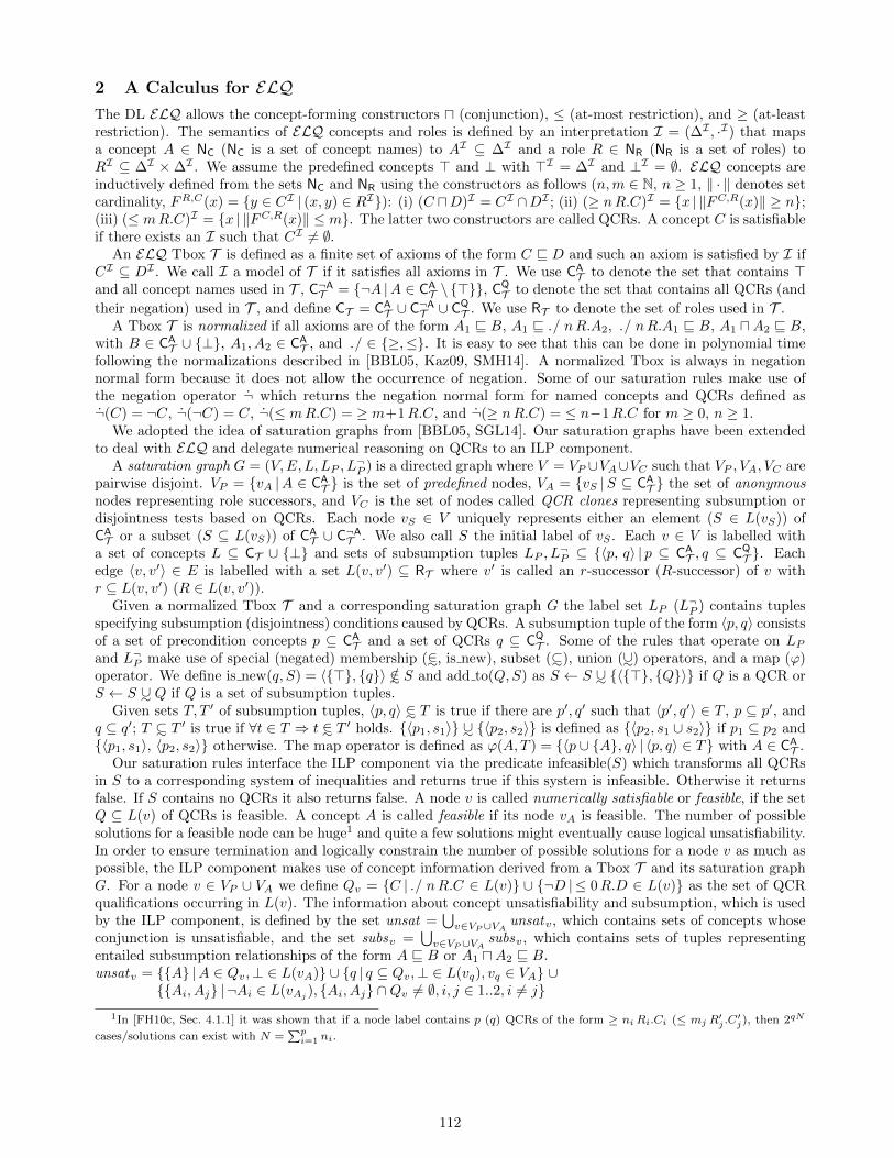
2 A Calculus for ELQThe DL ELQ allows the concept-forming constructors u (conjunction), ≤ (at-most restriction), and ≥ (at-leastrestriction). The semantics of ELQ concepts and roles is defined by an interpretation I = (∆I , ·I) that mapsa concept A ∈ NC (NC is a set of concept names) to AI ⊆ ∆I and a role R ∈ NR (NR is a set of roles) toRI ⊆ ∆I ×∆I . We assume the predefined concepts > and ⊥ with >I = ∆I and ⊥I = ∅. ELQ concepts areinductively defined from the sets NC and NR using the constructors as follows (n,m ∈ N, n ≥ 1, ‖ · ‖ denotes setcardinality, FR,C(x) = {y ∈ CI | (x, y) ∈ RI}): (i) (C uD)I = CI ∩DI ; (ii) (≥ nR.C)I = {x | ‖FC,R(x)‖ ≥ n};(iii) (≤ mR.C)I = {x | ‖FC,R(x)‖ ≤ m}. The latter two constructors are called QCRs. A concept C is satisfiableif there exists an I such that CI 6= ∅.

An ELQ Tbox T is defined as a finite set of axioms of the form C v D and such an axiom is satisfied by I ifCI ⊆ DI . We call I a model of T if it satisfies all axioms in T . We use CA

T to denote the set that contains >and all concept names used in T , C¬AT = {¬A |A ∈ CA

T \ {>}}, CQT to denote the set that contains all QCRs (and

their negation) used in T , and define CT = CAT ∪ C¬AT ∪ CQ

T . We use RT to denote the set of roles used in T .A Tbox T is normalized if all axioms are of the form A1 v B, A1 v ./ nR.A2, ./ nR.A1 v B, A1 uA2 v B,

with B ∈ CAT ∪ {⊥}, A1, A2 ∈ CA

T , and ./ ∈ {≥,≤}. It is easy to see that this can be done in polynomial timefollowing the normalizations described in [BBL05, Kaz09, SMH14]. A normalized Tbox is always in negationnormal form because it does not allow the occurrence of negation. Some of our saturation rules make use ofthe negation operator ¬ which returns the negation normal form for named concepts and QCRs defined as¬(C) = ¬C, ¬(¬C) = C, ¬(≤ mR.C) = ≥ m+1R.C, and ¬(≥ nR.C) = ≤ n−1R.C for m ≥ 0, n ≥ 1.

We adopted the idea of saturation graphs from [BBL05, SGL14]. Our saturation graphs have been extendedto deal with ELQ and delegate numerical reasoning on QCRs to an ILP component.

A saturation graph G = (V,E, L, LP , L¬P ) is a directed graph where V = VP ∪VA∪VC such that VP , VA, VC are

pairwise disjoint. VP = {vA |A ∈ CAT } is the set of predefined nodes, VA = {vS |S ⊆ CA

T } the set of anonymousnodes representing role successors, and VC is the set of nodes called QCR clones representing subsumption ordisjointness tests based on QCRs. Each node vS ∈ V uniquely represents either an element (S ∈ L(vS)) ofCAT or a subset (S ⊆ L(vS)) of CA

T ∪ C¬AT . We also call S the initial label of vS . Each v ∈ V is labelled witha set of concepts L ⊆ CT ∪ {⊥} and sets of subsumption tuples LP , L

¬P ⊆ {〈p, q〉 | p ⊆ CA

T , q ⊆ CQT }. Each

edge 〈v, v′〉 ∈ E is labelled with a set L(v, v′) ⊆ RT where v′ is called an r-successor (R-successor) of v withr ⊆ L(v, v′) (R ∈ L(v, v′)).

Given a normalized Tbox T and a corresponding saturation graph G the label set LP (L¬P ) contains tuplesspecifying subsumption (disjointness) conditions caused by QCRs. A subsumption tuple of the form 〈p, q〉 consistsof a set of precondition concepts p ⊆ CA

T and a set of QCRs q ⊆ CQT . Some of the rules that operate on LP

and L¬P make use of special (negated) membership (∈∼, is new), subset (⊂∼), union (∪∼) operators, and a map (ϕ)operator. We define is new(q, S) = 〈{>}, {q}〉 /∈∼ S and add to(Q,S) as S ← S ∪∼ {〈{>}, {Q}〉} if Q is a QCR orS ← S ∪∼ Q if Q is a set of subsumption tuples.

Given sets T, T ′ of subsumption tuples, 〈p, q〉 ∈∼ T is true if there are p′, q′ such that 〈p′, q′〉 ∈ T , p ⊆ p′, andq ⊆ q′; T ⊂∼ T

′ is true if ∀t ∈ T ⇒ t ∈∼ T′ holds. {〈p1, s1〉} ∪∼ {〈p2, s2〉} is defined as {〈p2, s1 ∪ s2〉} if p1 ⊆ p2 and

{〈p1, s1〉, 〈p2, s2〉} otherwise. The map operator is defined as ϕ(A, T ) = {〈p ∪ {A}, q〉 | 〈p, q〉 ∈ T} with A ∈ CAT .

Our saturation rules interface the ILP component via the predicate infeasible(S) which transforms all QCRsin S to a corresponding system of inequalities and returns true if this system is infeasible. Otherwise it returnsfalse. If S contains no QCRs it also returns false. A node v is called numerically satisfiable or feasible, if the setQ ⊆ L(v) of QCRs is feasible. A concept A is called feasible if its node vA is feasible. The number of possiblesolutions for a feasible node can be huge1 and quite a few solutions might eventually cause logical unsatisfiability.In order to ensure termination and logically constrain the number of possible solutions for a node v as much aspossible, the ILP component makes use of concept information derived from a Tbox T and its saturation graphG. For a node v ∈ VP ∪ VA we define Qv = {C | ./ nR.C ∈ L(v)} ∪ {¬D | ≤ 0R.D ∈ L(v)} as the set of QCRqualifications occurring in L(v). The information about concept unsatisfiability and subsumption, which is usedby the ILP component, is defined by the set unsat =

⋃v∈VP∪VA

unsatv, which contains sets of concepts whoseconjunction is unsatisfiable, and the set subsv =

⋃v∈VP∪VA

subsv, which contains sets of tuples representingentailed subsumption relationships of the form A v B or A1 uA2 v B.unsatv = {{A} |A ∈ Qv,⊥ ∈ L(vA)} ∪ {q | q ⊆ Qv,⊥ ∈ L(vq), vq ∈ VA} ∪

{{Ai, Aj} | ¬Ai ∈ L(vAj ), {Ai, Aj} ∩Qv 6= ∅, i, j ∈ 1..2, i 6= j}1In [FH10c, Sec. 4.1.1] it was shown that if a node label contains p (q) QCRs of the form ≥ ni Ri.Ci (≤ mj R

′j .C

′j), then 2qN

cases/solutions can exist with N =∑p

i=1 ni.

112

subsv = {〈{A1, A2}, B〉 | {A1, A2} ⊆ Qv, C1 u C2 v D ∈ T , Ci ∈ L(vAi), B ∈ L(vD), i ∈ 1..2} ∪

{〈{A}, B〉 |B ∈ L(vA), A ∈ Qv}In case a node v is numerically satisfiable, the set σ(v) contains solutions for feasible inequality systems

denoted by the QCRs in L(v). A QCR solution is described by a set of tuples of the form 〈r, q, n〉 with r ⊆ RTand q ⊆ CA

T ∪C¬AT sets of roles and concepts respectively, and n denotes the cardinality of the set of r-successorsthat are instances of all concepts contained in q.

A saturation graph G is initialized with representative nodes for all concepts in CAT . For instance, for a concept

A a node vA is created with L(vA) = {>, A} and LP (vA) = L¬P (vA) = ∅. The saturation rules are applied to aninitialized saturation graph until no rule is applicable anymore. Only the vP4

-Rule and v¬P4-Rule with v ∈ VC

can be applied to a node v if ⊥ ∈ L(v).This algorithm computes the named subsumers for all predefined nodes and, thus, decides satisfiability and

subsumption for all concepts in CAT . A concept A is satisfiable iff ⊥ /∈ L(vA), and A is subsumed by B iff

B ∈ L(vA). The top section of Figure 1 contains five rules. The v-Rule (v¬-Rule) allows a QCR or namedconcept on its right-hand (left-hand) side. Thev∗-Rule ensures that L(v) contains all QCRs and (negated) namedconcepts inherited from its subsumers. The vu-Rule is a standard EL rule complemented by its contrapositiveversion (v¬u-Rule). The second section contains two rules that deal with role successors where # denotes thecardinality of an anonymous node. If 〈r, q, n〉 ∈ σ(v) the fil-rule and e-rule ensure that an edge r ⊆ L(v, vq)exists that connects v to an anonymous successor vq with L(vq) = q and #vq = n, i.e., vq represents n identicalr-successors of v.

For a node v the ⊥-Rule records clashes by adding ⊥ to L(v). For a node v′ created by the fil-rule there isno need to propagate ⊥ to its predecessor v because v′ represents one of possibly many existing QCR solutionsfor v. If all QCR solutions for v fail, the ILP component eventually determines that v is infeasible and thusunsatisfiable.

The fourth section of Figure 1 contains five rules that create and maintain subsumption tuples. Only threeof these rules (P./-Rule, P¬./-Rule, Pu-Rule) derive tuples from axioms. The other two rules propagate tuples up(vP -Rule) or down (v¬P -Rule) the subsumption hierarchy.

The bottom section of Figure 1 lists rules that discover subsumptions or disjointness due to subsumptiontuples. Q(v, S) is defined as

⋃〈p,q〉∈S{q | p ⊆ L(v)} and contains applicable QCRs selected from the set S of

subsumption tuples. The relation clone ⊆ V × (CAT ∪ C¬AT )× V keeps track of subsumption or disjointness tests

and their associated QCR clones. For instance, a QCR clone v′ ∈ VC of vA contains all QCRs contained inL(vA) and LP (vB) (L¬P (vB)) and represents the test whether A is subsumed by (disjoint to) B. If v′ becomesunsatisfiable, then B (¬B) is added to L(vA). The vP1

-Rule creates necessary QCR clones, the vP2-Rule (vP3

-Rule) ensures that Q(vA, LP (vB)) (L(vA) ∩ CQ

T ) is contained in L(v′). The vP4-Rule adds B to L(vA) if vA’s

corresponding clone is unsatisfiable. The other four rules deal with disjointness in an analogous way.

3 Small Tbox Example Illustrating Rule Application

We demonstrate our calculus with a small ALCQ Tbox T which entails C v D1 u ¬D2 (see below). A slightlydifferent example (C-SAT-exp-ELQ) is also used in our synthetic benchmark (see Section 6) and surprisinglynone of the tested reasoners besides Avalanche and Racer can classify the version with n = 10 within a timelimit of 1000 seconds.C v ≥ 20R.> u≤ 10R.A u ≤ 10R.BC v D1 tD2

D1 v ≤ 10R.¬A, D2 v ≤ 9R.¬BThe following steps show our rewriting of T into T ′, which is a normalized ELQ Tbox that is a conservativeextension of T .

1. We remove the occurrence of t and add the entailment C v D1 t D2 using fresh concepts X3, X4 and afresh role S1.C v ≥ 20R.> u≤ 10R.A u ≤ 10R.BC u ≥ 1S1.(X3 uX4) v D1

C u ≥ 2S1.> v D2

}These two axioms entail C v D1 tD2

D1 v ≤ 10R.¬AD2 v ≤ 9R.¬B

2. We normalize the axioms (but allow a conjunction on the right-hand side for sake of brevity) and replace¬A,¬B by notA,notB and new axioms using fresh roles S2, S3 such that ¬notA v A and ¬notB v B are

113

v-Rule if A v φ ∈ T , φ /∈ L(vA)then add φ to L(vA)

v¬-Rule if φ v A ∈ T ,¬A ∈ L(v), ¬φ /∈ L(v)then add ¬φ to L(v)

v∗-Rule if A ∈ L(v), τ ∈ L(vA), τ /∈ L(v)then add τ to L(v)

vu-Rule if A1 uA2 v B ∈ T , {A1, A2} ⊆ L(v), B /∈ L(v)then add B to L(v)

v¬u-Rule if Ai uAj v B ∈ T , {¬B,Ai} ⊆ L(v),¬Aj /∈ L(v)then add ¬Aj to L(v)

fil-Rule if 〈r, q, n〉 ∈ σ(v),¬∃ vq ∈ V : q ⊆ L(vq),#vq ≥ nthen create vq ∈ VA with L(vq)← q and #vq ← n

e-Rule if 〈r, q, n〉 ∈ σ(v), q ⊆ L(vq),#vq ≥ n, r * L(v, vq)then add r to L(v, vq)

⊥-Rule if ⊥ /∈ L(v) ∧ (infeasible(L(v)) ∨ {A,¬A} ⊆ L(v))then add ⊥ to L(v)

P./-Rule if ./ nR.A v B ∈ T , is new(¬(./ nR.A), LP (vB))then add to(¬(./ nR.A), LP (vB))

P¬./-Rule if A v ./ nR.B ∈ T , is new(./ nR.B,L¬P (vB))then add to(./ nR.B,L¬P (vB))

P -Rule if B ∈ L(vA), LP (vA) 6⊂∼ LP (vB)then add to(LP (vA), LP (vB))

P¬-Rule if B ∈ L(vA), L¬P (vB) 6⊂∼ L¬P (vA)

then add to(L¬P (vB), L¬P (vA))Pu-Rule if Ai uAj v B ∈ T , ϕ(Ai, LP (vAj

)) 6⊂∼ LP (vB)then add to(ϕ(Ai, LP (vAj

)), LP (vB))

vP1-Rule if Q(v, LP (vB)) 6= ∅, {B,¬B} ∩ L(v) = ∅, clone(v,B) = ∅

then create v′ ∈ VC , L(v′)← {>}, clone(v,B)← {v′}vP2 -Rule if v′ ∈ clone(v,B), {B,¬B} ∩ L(v) = ∅, Q(v, LP (vB)) * L(v′)

then add to(Q(v, LP (vB)), L(v′))

vP3-Rule if v′ ∈ clone(v,B), {B,¬B} ∩ L(v) = ∅, L(v) ∩ CQ

T * L(v′) ∩ CQT

then add to(L(v) ∩ CQ, L(v′))vP4

-Rule if {B,¬B} ∩ L(v) = ∅, v′ ∈ clone(v,B),⊥ ∈ L(v′)then add B to L(v)

v¬P1-Rule if Q(v, L¬P (vB)) 6= ∅, {B,¬B} ∩ L(v) = ∅, clone(v,¬B) = ∅

then create v′ ∈ VC , L(v′)← {>}, clone(v,¬B)← {v′}v¬P2

-Rule if v′ ∈ clone(v,¬B), {B,¬B} ∩ L(v) = ∅, Q(v, L¬P (vB)) * L(v′)then add to(Q(v, L¬P (vB)), L(v′))

v¬P3-Rule if v′ ∈ clone(v,¬B), {B,¬B} ∩ L(v) = ∅, L(v) ∩ CQ

T * L(v′) ∩ CQT

then add to(L(v) ∩ CQ, L(v′))vP¬4

-Rule if {B,¬B} ∩ L(v) = ∅, v′ ∈ clone(v,¬B),⊥ ∈ L(v′)then add ¬B to L(v)

Figure 1: Saturation rules (φ ∈ CAT ∪ CQ

T , τ ∈ CT ; ./ ∈ {≥,≤}; i, j ∈ 1..2, i 6= j)

114

entailed. This Tbox T ′ additionally entails C v X5 u ¬X7.C v ≥ 20R.> u≤ 10R.A u ≤ 10R.BC uX5 v D1

≥ 1S1.X6 v X5

X3 uX4 v X6

C uX7 v D2

≥ 2S1.> v X7

D1 v ≤ 10R.notAD2 v ≤ 9R.notB≤ 1S2.> v notA≥ 1S2.> v A

}These two axioms entail ¬notA v A

≤ 1S3.> v notB≥ 1S3.> v B

}These two axioms entail ¬notB v B

3. Known subsumptions or unsatisfiability of concept conjunctions are derived from T ′.subs = {〈{C,X5}, D1〉, 〈{C,X7}, D2〉, 〈{X3, X4}, X6〉}unsat = ∅

4. After applying the rules v, P./, P¬./, Pu we get the following node labels (for sake of better readability wedenote vA, where A is a concept name, simply as A when used for the labels L,LP , L

¬P ; anonymous and

clone nodes are denoted as vaiand vcj respectively).

L(C) = {>, C,≥ 1S1.X3,≥ 1S1.X4,≥ 20R.>,≤ 10R.A,≤ 10R.B}σ(C) = {〈{R}, {¬A,¬B,¬notB}, 20〉, 〈{S1}, {X3, X4, X6}, 1〉}L¬P (C) = {〈{>}, {≥ 1S1.X3}〉, 〈{>}, {≥ 1S1.X4}〉, 〈{>}, {≥ 20R.>}〉, 〈{>}, {≤ 10R.A}〉,

〈{>}, {≤ 10R.B}〉}L(D1) = {>, D1,≤ 10R.notA}L¬P (D1) = {〈{>}, {≤ 10R.notA}〉}LP (D1) = {〈{>, C}, {≤ 0S1.X6}〉L(D2) = {>, D2,≤ 9R.notB}L¬P (D2) = {〈{>}, {≤ 9R.notB}〉}LP (D2) = {〈{>, C}, {≤ 1S1.>}〉LP (X5) = {〈{>}, {≤ 0S1.X6}〉}LP (X7) = {〈{>}, {≤ 1S1.>}〉}LP (notA) = {〈{>}, {≥ 2S2.>}〉}LP (A) = {〈{>}, {≤ 0S2.>}〉}LP (notB) = {〈{>}, {≥ 2S3.>}〉}LP (B) = {〈{>}, {≤ 0S3.>}〉}

5. After applying the rules v¬P1, v¬P2

, v¬P3(is C disjoint to D2?) and creating the clone vc1

clone(C,¬D2)← vc1L(vc1) = {>,≥ 1S1.X3,≥ 1S1.X4,≥ 20R.>,≤ 10R.A,≤ 10R.B,≤ 9R.notB}

6. After applying the fil- and e-rule for vc1 and the rules v¬, ⊥ for va1

σ(vc1) = {〈{R}, {¬A,¬B,¬notB}, 20〉, 〈{S1}, {X3, X4, X6}, 1〉}L(vc1 , va1) = {R}L(va1

) = {>,¬A,¬B,¬notB ,≤ 0S2.>,≤ 0S3.>,≥ 2S3.>,⊥}, #va2= 20

L(vc1 , va2) = {S1}

L(va2) = {>, X3, X4, X6}, #va2

= 1Based on the unsatisfiability of va1 we add {¬A,¬B,¬notB} to unsat .

7. After applying the fil- and e-rule for vc1 again, the rules v¬, ⊥ for va3

σ(vc1) = {〈{R}, {¬A,¬B,notB}, 9〉, 〈{R}, {¬A,B,¬notB}, 1〉, 〈{R}, {A,¬B,¬notB}, 10〉,〈{S1}, {X3, X4, X6}, 1〉}

L(vc1 , va3) = {R}

L(va3) = {>,¬A,¬B,notB ,≤ 0S2.>,≤ 0S3.>}, #va3

= 9L(vc1 , va4) = {R}L(va4) = {>,¬A,B,¬notB ,≤ 0S2.>,notA,≥ 2S3.>}, #va4 = 1

115

L(vc1 , va5) = {R}

L(va5) = {>, A,¬B,¬notB ,≤ 0S3.>,notB ,⊥}, #va2

= 10Based on the unsatisfiability of va5

we add {A,¬B,¬notB} to unsat . Together with the previous additionto unsat we learned that {¬B,¬notB} is unsatisfiable.

8. The ⊥-rule adds ⊥ to L(vc1) because infeasible(L(vc1)) is true due to {¬B,¬notB} ∈ unsat .

9. The v¬P4-rule adds ¬D2 to L(C).

10. The rules v¬u and v¬ add ¬X7 and ≤ 1S1.> to L(C).

11. After applying the rules vP1, vP2

, vP3(is C subsumed by X5?) and creating the clone vc2

clone(C,X5)← vc2L(vc2) = {>,≥ 1S1.X3,≥ 1S1.X4,≥ 20R.>,≤ 10R.A,≤ 10R.B,≤ 1S1.>,≤ 0S1.X6}

12. The ⊥-rule adds ⊥ to L(vc2) because infeasible(L(vc2)) is true due to role S1.

13. The vP4-rule adds X5 to L(C).

14. The vu-rule adds D1 to L(C).

Other rules are still applicable but for sake of brevity we do not illustrate their application. Furthermore, noother concept subsumptions are entailed w.r.t. T .

4 ILP Component

We now present the large-scale optimization framework we have designed for solving the system of QCRs inthe DL ELQ. It is based on a decomposition technique, called DantzigWolfe decomposition or more commonlycolumn generation technique [Las70, Chv83], combined with a branch-and-price technique [BJN+98] in order toeither detect that the system is infeasible, or to compute an optimal solution of the system.

Given T , v ∈ V and S containing QCRs, define the qualifying role set of v as SQ = {α(./ nR.C) | ./ nR.C ∈S} ∪ {C | ./ nR.C ∈ S} ∪ {>,⊥}, where α defines a mapping between a QCR and its associated (proxy) subroleof R that is new in T , e.g., α(./ nR.C) = R′ with R′ v R and R′ new in T . The role partitioning PSQ

of aqualifying role set SQ is defined as the power set of SQ (without the empty set). Note that a qualifying conceptcan be a member of a partition only if the partition also contains at least one role. For each partition p ∈ PSQ

,we define pI = fil(v, p)∩ (∆I \

⋃Y ∈SQ\p fil(v, Y )) where fil(v, p) =

⋂e∈p fil(v, e) and fil(v, e) = eI if e is a concept

and fil(v, e) = {yI | (vI , yI) ∈ eI} if e is a role. The semantics of role partitions in PSQis defined in such a

way that their interpretations are pairwise disjoint. The absence of a role or concept in a partition implies thepresence of its semantic negation. We now define a mapping ξ from S to a linear inequality system as follows:

- ξ(≥ nR.C) = {∑

q∈PSQ|R′∈q xq ≥ n} with R′ = α(≥ nR.C),

- ξ(≤ nR.D) = {∑

q∈PSQ|R′′∈q xq ≤ n} ∪

⋃q∈Q{xq ≤ 0}, such that Q = {p ∈ PSQ

|D ∈ p ∧ R′′ /∈ p}, with

R′′ = α(≤ nR.D).

In order to determine whether ξ(S) =⋃

./nR.C∈S ξ(./ nR.C) is feasible using a highly scalable solution, wepropose a column generation ILP formulation for expressing ξ(S) as a mathematical ILP model, which will besolved using a branch-and-price algorithm [BJN+98].

Given T , v ∈ V , S, SQ and PSQ, the ILP model associated with the feasibility problem of ξ(S) can be written

as follows:

min∑

p∈PSQ

costpxp (1)

subject to:∑

p∈PSQ

aR′

p xp ≥ δR′ R′ ∈ S≥roleQ (2)

∑p∈PSQ

aR′

p xp ≤ δR′ R′ ∈ S≤roleQ (3)

xp ∈ Z+ p ∈ PSQ, (4)

116

where S≥roleQ = {α(≥ nR.C) | ≥ nR.C ∈ S}, S≤roleQ = {α(≤ nR.C) | ≤ nR.C ∈ S}, SroleQ = S≥roleQ ∪ S≤roleQ ,

δR′ (δR′) is the cardinality of an at-least (at-most) restriction on a subrole R′ ∈ SroleQ , and xp represents a

partition of the set PSQ. costp is defined as the number of concepts in partition p.

When the set of inequalities has a non empty solution set, we are interested in partitions that only contain theentailed concepts, i.e., the minimum number of concepts that are needed to satisfy all the axioms. Consequently,in the objective, costp ensures that output partitions only contain the entailed concepts, i.e., the minimumnumber of concepts that are needed to satisfy all the axioms.

In order to design a scalable solution of (1)-(4), which has an exponential number of variables, we considera solution scheme that makes use of an implicit representation of the constraint matrix. This corresponds tousing a branch-and-price method, a generalization of a branch-and-bound method [NW88] in which the linearrelaxation of (1)-(4) is solved with a column generation algorithm ([Las70], [Chv83]). The linear relaxation isdefined by (1)-(3) and constraint (4′), which is written as follows:

xp ∈ R+ p ∈ PSQ. (4′)

Next step is to use an implicit representation of all the variables of (1)-(4′). Therefore, instead of defining thevariables for p ∈ PSQ

, we do it for p ∈ P ′SQ⊆ PSQ

, leading to the so-called restricted ILP or restricted master

problem in the mathematical programming literature, in which constraints (4′) are replaced by constraints

xp ∈ R+ p ∈ P ′SQ, (4′′)

with P ′SQ= ∅ at the outset. We next have an iteration solution process in which, at each iteration, the column

generation algorithm tries to generate an improving partition p, i.e., a partition such that, if added to the currentP ′SQ

, improves the objective of formulation (1)-(4′′). The partition generator (PG), also called pricing problemin the mathematical programming literature, is a mathematical ILP model with two sets of decision variables:aR′

= 1 if role R′ is in the generated partition, 0 otherwise ; bC = 1 if concept C ∈ SconceptQ is in the generated

partition, 0 otherwise, where SconceptQ containing all the concepts of SQ and no subrole. The (PG) model can be

stated as:

(PG) min∑

C∈SconceptQ

bC −∑

R′∈S≥roleQ

aR′πR′ −

∑R′∈S≤role

Q

aR′ωR′ (5)

subject to: aR′≤ bC R′ ∈ S≥roleQ , C = R′.qualifier (6)

bC ≤ aR′

R′ ∈ S≤roleQ , C = R′.qualifier (7)

bC ≤ b> C ∈ SconceptQ (8)

b⊥ = 0 (9)

bC , aR′ ∈ {0, 1} R′ ∈ Srole

Q , C ∈ SconceptQ = SQ \ Srole

Q , (10)

where πR′ and ωR′ are the optimal values of the dual variables of problem (1)-(4′′) (see [Chv83] if not familiarwith linear programming concepts). The objective function (5) is the so-called reduced cost of a partition (orcolumn, see again [Chv83] for more details on the column generation method). Constraints (6)-(10) implementthe semantics of ξ(S).

(PG) returns a valid partition of PSQ, assuming no other information is provided. In its feasibility space, it

contains a 1-to-1 mapping between the said partitions and algebraic inequalities. If other informations such as:(i) subsumption (T |= A v B), (ii) binary subsumption (AuB v C) and (iii) disjointness (T |= A1 u · · · uAn v⊥, n ≥ 1) are provided, the cardinality of some partitions p ∈ PSQ

might need to be 0. Depending on theinformation received, the semantics can be implemented by (in)equalities, using a 1-to-1 mapping presentedbelow.

- For every T |= A v B, set SconceptQ = Sconcept

Q ∪ {A,B} and add bA ≤ bB to (PG), in order to guaranteethat if a generated partition contains a certain concept, it does contain all its subsumers.

- For every T |= A u B v C, update SconceptQ = Sconcept

Q ∪ {A,B,C} and add bA + bB − 1 ≤ bC to (PG).Then, if (PG) generates a partition containing A and B, it must contain C as well.

- For every disjointness relation T |= A1 u · · · u An v ⊥, n ≥ 1, set SconceptQ = Sconcept

Q ∪ {A1, . . . , An} and

add∑n

i=1 bAi− n + 1 ≤ b⊥ to (PG). This inequality ensures that if all the concepts Ai, i = 1, . . . , n are

present in a partition; this partition cannot be generated since otherwise it would contain ⊥ as well.

117

Figure 2: Overview of ILP solution process

- If there is some concept C with ¬C ∈ SconceptQ , the relationship of C and ¬C can be modelled with equality

bC + b¬C = 1. This implies that every generated partition contains exactly one of C and ¬C.

Every partition generated by (PG), which possibly contains some of the above inequalities or equalities,satisfies all the input axioms except the QCRs, which are taken care of in (1)-(4′′). The column generationmethod is an iterative process in which (1)-(4′′) and (PG) are alternatively solved until (PG) cannot provide anynew improving partitions, i.e., when the optimal value of the objective of (PG) is positive. This corresponds toone of the optimality conditions when solving a linear program, see, e.g., [Chv83] for more details.

In the branch-and-price algorithm, an implicit enumeration scheme with a breadth first search (BFS) explo-ration strategy, branching is done upon a subrole R′∗ selected as follows:

R′∗ = arg maxR′∈Srole

Q

∑p∈P′

aR′

p ×max {xp − bxpc, dxpe − xp}

, (11)

leading to two branches, one with aR′∗

= 0 and the other one with aR′∗

= 1. This branching scheme is clearlyexhaustive and valid (see [Van11] and [NW88]). The branch-and-price algorithm terminates when either aninteger feasible solution for (1)-(4) is found, or an infeasibility is detected, i.e., either the linear programmingrelaxation (1)-(4′′) has no solution (in most of the infeasibility cases) or the branch-and-price algorithm failsto find a feasible integer solution, see [NW99]. A flowchart is provided in Figure 2 to summarize the solutionprocess.

Soundness and Completeness

The mapping presented in the previous paragraphs is a one-to-one mapping between the axioms and the algebraicinequalities. Thus, the feasibility space defined by (2)-(4) represents all the instances that satisfy all axioms.Following the decomposition ILP model that is proposed, constraints related to satisfying QCRs are addressedin (2)-(4), while all other axioms are embedded in (PG). The branch-and-price algorithm, if (1)-(4) is feasible,returns one set of valid partitions, and the selection of them is made by the objective (1).

118

The result of the proposed solution process is sound. Indeed, every model produced by the large-scale opti-mization framework, i.e., ILP model (1)-(4) and branch-and-price algorithm, satisfies all the axioms that are fedto the ILP component. It is also complete, because the feasibility spaces of the (1)-(4′′) and (PG) consider allthe possible models through the one-to-one mapping that leads to ILP model (1)-(4). In addition, the branchingrule in the branch-and-price algorithm considers a partitioning of the overall solution space, therefore no solutionis left out.

5 Soundness and Completeness

Due to lack of space we can only sketch the soundness and completeness proofs for our saturation rules. Giventhe presentation in the previous section we know that the algorithms implementing the ILP component aresound and complete and terminate in finite time for deciding whether a set of QCRs is feasible, i.e., numericallysatisfiable.

Intuitively speaking our soundness proof is an extension of the one for EL but all subsumptions or disjointnessinvolving QCRs are based on QCR infeasibility tests performed by the ILP component. Once a subsumption ordisjointness has been proven, its evidence as an element of a node label becomes part of the saturation graph.Since QCRs can interact with one another a QCR solution and its corresponding model is not proof enough fora subsumption unless it is known to be the only possible solution. In order to test QCR-based entailment thelabel sets LP and L¬P of potential (non-)subsumer nodes together with node labels are used for a feasibility test.If such a set of QCRs has been proven to be infeasible, the corresponding subsumption or disjointness can beadded to the graph. Thus, only entailed subsumptions or disjointness will be inferred.

Lemma (Soundness). Let G be the saturation graph for a normalized Tbox T after the application of all satu-ration rules in Figure 1 has terminated and C ∈ CA

T and D ∈ CAT ∪ {⊥}, β ∈ {D, ¬D}. Then T |= C v β if it

holds that β ∈ L(vC).

Proof. Let us assume that each rule application creates a new saturation graph and the sequence of rule applica-tions until termination produce a sequence of graphs G1, . . . , Gm with Gi = (Vi, Ei, Li, LP iL

¬P i) and i ∈ 1..m. Let

FR,C(x) = {y ∈ CI | (x, y) ∈ RI}, and Q(v, S) =⋃〈p,q〉∈S{q | p ⊆ L(v)}. For all m ∈ N, models I of T , r ⊆ RT ,

and x ∈ CI we claim the following holds: (i) if β ∈ Lm(vC) then T |= C v β; (ii) if r ⊆ Lm(vC , vq),#vq ≥ n

then there exist yi ∈ ∆I with (x, yi) ∈⋂

R∈r RI , yi ∈

⋂q′∈q q

′I , i ∈ 1..n.We prove our claim by induction on m. We start with m = 0 and assume that I is a model for T . For G0 we

have L0(vC) = {>, C}, L0(vC , vD) = ∅ implying that D = C. It is trivial to see that our claim holds. For theinduction step we make a case distinction according to applicable rules.

v-Rule Let φ ∈ Lm(vC) \ Lm−1(vC) and x ∈ CI . Then there exists C ∈ Lm−1(vC) and C v φ ∈ T . Since I amodel of T it holds x ∈ φI .

v¬-Rule Let ¬φ ∈ Lm(v) \ Lm−1(v) and x ∈ ∆I \ CI . Then there exists ¬C ∈ Lm−1(vC) and φ v C ∈ T .Since I a model of T it holds x ∈ ∆I \ φI .

v∗-Rule Let τ ∈ Lm(v)\Lm−1(v) and x ∈ CI . Then there exists τ ∈ Lm−1(vC) and CI ⊆ τI . Since I a modelof T it holds x ∈ τI .

vu-Rule Let D ∈ Lm(v) \ Lm−1(v) and x ∈ CI1 , x ∈ CI2 . Then there exists C1, C2 ∈ Lm−1(v) and C1 u C2 vD ∈ T . Since I a model of T it holds x ∈ CI1 ∩ CI2 and thus x ∈ DI .

v¬u-Rule Let ¬Cj ∈ Lm(v) \ Lm−1(v) and x ∈ ∆I \ DI , x ∈ CIi . Then there exists ¬D,Ci ∈ Lm−1(v) andCi u Cj v D ∈ T . Since I a model of T it holds x ∈ CIi ∪ (∆I \ CIj ) ∪ (∆I \DI) and thus x ∈ ∆I \ CIj .

fil-Rule, e-Rule Let vq ∈ Vm \Vm−1, r ⊆ Lm(vC , vq) such that q ⊆ Lm(vq) and #vq ≥ n, Q = Lm−1(vC)∩CQT ,

and let x ∈⋂

q′∈Q q′I . Due to the soundness and completeness of the ILP component and since I is

a model of T , w.l.o.g. we can assume that that a solution 〈r, q, n〉 ∈ σ(vC) exists and we have yi with

(x, yi) ∈⋂

R∈r RI , yi ∈

⋂q′∈q q

′I with i ∈ 1..n, and it holds ∀q′ ∈ Q : x ∈ q′I .

⊥-Rule Let ⊥ ∈ Lm(vC) \ Lm−1(vC), then either {A,¬A} ⊆ Lm−1(vC) and x ∈ AI , x ∈ ∆I \ AI orinfeasible(Lm−1(vC)) and by the soundness of the ILP component x ∈

⋂q∈Lm−1(vC)∩CQ

TqI . In both cases it

holds that x ∈ ⊥I .

119

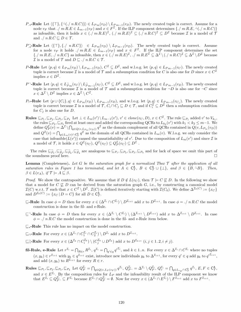
P./-Rule Let 〈{>}, {¬(./ nR.C)}〉 ∈ LPm(vD) \LPm−1(vD). The newly created tuple is correct. Assume for anode vF that ./ mR.E ∈ Lm−1(vF ) and x ∈ F I . If the ILP component determines {./ mR.E, ¬(./ nR.C)}as infeasible, then it holds x ∈ (./ mR.E)I , (./ mR.E)I ⊆ (./ nR.C)I ⊆ DI because I is a model of Tand ./ nR.C v D ∈ T .

P¬./-Rule Let 〈{>}, {./ nR.C}〉 ∈ LPm(vD) \ LPm−1(vD). The newly created tuple is correct. Assumefor a node vF it holds ./ mR.E ∈ Lm−1(vF ) and x ∈ F I . If the ILP component determines the set{./ mR.E, ./ nR.C} as infeasible, then x ∈ (./ mR.E)I , ./ mR.EI ⊆ ∆I \ (./ nR.C)I ⊆ ∆I \DI becauseI is a model of T and D v ./ nR.C ∈ T .

P -Rule Let 〈p, q〉 ∈ LPm(vD) \ LPm−1(vD), CI ⊆ DI , and w.l.o.g. let 〈p, q〉 ∈ LPm−1(vC). The newly createdtuple is correct because I is a model of T and a subsumption condition for C is also one for D since x ∈ CIimplies x ∈ DI .

P¬-Rule Let 〈p, q〉 ∈ L¬Pm(vC)\L¬Pm−1(vC), CI ⊆ DI , and w.l.o.g. let 〈p, q〉 ∈ LPm−1(vD). The newly createdtuple is correct because I is a model of T and a subsumption condition for ¬D is also one for ¬C sincex ∈ ∆I \DI implies x ∈ ∆I \ CI .

Pu-Rule Let 〈p ∪ {Ci}, q〉 ∈ LPm(vD) \ LPm−1(vD), and w.l.o.g. let 〈p, q〉 ∈ LPm−1(vCj). The newly created

tuple is correct because I is a model of T , Ci uCj v D ∈ T , and if CIi ⊆ DI then a subsumption conditionfor Cj is also one for D.

Rules vP1,vP2

,vP3,vP4

Let ⊥ ∈ Lm(v′)\Lm−1(v′), v′ ∈ clone(vC , D), x ∈ CI . The rule vP1added v′ to Vk1

,the rulesvP2 ,vP3 fired at least once and added the corresponding QCRs to Lk2(v′) with k1 < k2 ≤ m−1. Wedefine QIP (v) = ∆I \

⋂q∈Q(v,LPm (vD)) q

I as the domain complement of all QCRs contained in Q(v, LPm(vD))

and QI(v) =⋂

q∈Lm(v)∩CQTqI as the domain of all QCRs contained in Lm(v). W.l.o.g. we only consider the

case that infeasible(L(v′)) caused the unsatisfiability of v′. Due to the composition of Lm(v′) and since I isa model of T , it holds x ∈ QI(vC), QI(vC) ⊆ QIP (vC) ⊆ DI .

The rules v¬P1,v¬P2

,v¬P3,v¬P4

are analogous to vP1,vP2

,vP3,vP4

and for lack of space we omit this part ofthe soundness proof here.

Lemma (Completeness). Let G be the saturation graph for a normalized Tbox T after the application of allsaturation rules in Figure 1 has terminated, and let A ∈ CA

T , B ∈ CAT ∪ {⊥}, and β ∈ {B, ¬B}. Then,

β ∈ L(vA), if T |= A v β.

Proof. We show the contrapositive. We assume that if D /∈ L(vC), then T |= C 6v D. In the following we showthat a model for C 6v D can be derived from the saturation graph G, i.e., by constructing a canonical modelI(C) w.r.t. T such that x ∈ CI \DI . I(C) is defined iteratively starting with I(C0). We define ∆I0(C) := {xC}and DI0(C) := {xC |D = C} for all D ∈ CA

T .

v-Rule In case φ = D then for every x ∈ (∆Ii ∩ CIi) \DIi+1 add x to DIi+1 . In case φ = ./ nR.C the modelconstruction is done in the fil- and e-Rule.

v¬-Rule In case φ = D then for every x ∈ (∆Ii \ CIi) \ (∆Ii+1 \ DIi+1) add x to ∆Ii+1 \ DIi+1 . In caseφ = ./ nR.C the model construction is done in the fil- and e-Rule item below.

v∗-Rule This rule has no impact on the model construction.

vu-Rule For every x ∈ (∆Ii ∩ CIi1 ∩ CIi2 ) \DIi add x to DIi+1 .

v¬u-Rule For every x ∈ (∆Ik ∩ CIki ) \ (CIkj ∪DIk) add x to DIk+1 (i, j ∈ 1..2, i 6= j).

fil-Rule, e-Rule Let rIi =⋂

R∈r RIi , qIi =

⋂q′∈q q

′Ii , and k ∈ 1..n. For every x ∈ ∆Ii ∩ CIi where no tuples

(x, yk) ∈ rIi+1 with yk ∈ qIi+1 exist, introduce new individuals yk to ∆Ii+1 , for every q′ ∈ q add yk to q′Ii+1 ,

and add (x, yk) to RIi+1 for every R ∈ r.

Rules vP1 ,vP2 ,vP3 ,vP4 Let QIiP =⋂

q∈Q(v,LP (vF )) qIi , QIiP¬ = ∆Ii \ QIiP , QIiv =

⋂q∈LvE

∩CQTqIi , E,F ∈ CA

T ,

and x ∈ EIi . By the composition rules for LP and the infeasibility result of the ILP component we knowthat EIi ⊆ QIiP¬ ⊆ F Ii because EIi ∩QIiP = ∅. Now for every x ∈ (∆Ii ∩ EIi) \ F Ii+1 add x to F Ii+1 .

120

The rules v¬P1,v¬P2

,v¬P3,v¬P4

are analogous to vP1,vP2

,vP3,vP4

and for lack of space we omit this part ofthe completeness proof here.

The construction of a model is performed in a fair manner, i.e., every rule applicable to already existingelements in ∆Ii is applied before applying rules to new elements. The constructed model I(C) is indeed a modelof C w.r.t T . Due to lack of space we cannot prove this in detail but we argue informally. Although our rules dealwith ELQ, a subset of these deal with EL if one assumes that only QCRs of the form ≥ 1R.C are allowed. Thus,we claim that our rules are complete for EL. Due to the semantics of QCRs and their allowed occurrence on theleft- and and right-hand side of axioms, these can entail subsumptions that are not possible in EL. In order toensure completeness we introduced the labels LP and L¬P that aggregate possible (non-)subsumption conditionscaused by QCRs. In order to prove subsumption or disjointness we create corresponding QCR clones. In casea clone is satisfiable after all rules have terminated this clone can serve as a model for the non-subsumptionor non-disjointness. In case additional entailed information is added to the saturation graph that causes theunsatisfiability of a QCR clone, we will add the entailed subsumption or disjointness to the sets subs andunsat that are used by the ILP component. Regarding the fil- and e-rule there could exist another possibleincompleteness because a numerically satisfiable set of QCRs could eventually cause the unsatisfiability of acreated anonymous node due to entailed information missing in the graph at the time of the feasibility test.However, if such an anonymous node becomes unsatisfiable, the cause of unsatisfiability is learned by adding itscause to the sets subs and unsat . This ensures that a previously computed solution is monotonically constraineduntil either an anonymous node is determined as satisfiable or the set of QCRs becomes eventually infeasible.Again, this ensures that no model for non-subsumption or non-disjointness is overlooked and no subsumption ordisjointness is missed.

Lemma (Termination). For every normalized ELQ Tbox over CT and RT the application of the saturation rulesin Figure 1 will terminate in finite time.

Proof. The algorithm terminates naturally because the saturation graph is finite and its number of nodes isbounded by the size of the power set of CT and RT respectively, cycles are avoided by reusing nodes in accordanceto standard subset blocking. Finally, the number of concepts, edges, QCRs, and subsumption tuples that canbe added to L, LP , and L¬P is again bounded by the size of the power set of CT and RT respectively. All rulesextend labels monotonically. Once the precondition of a rule is true for elements of a graph G and the rule hasfired, it cannot fire again for the same set of elements, thus, any series of rule applications is finite.

6 A First Experimental Evaluation

We developed a prototype system called Avalanche that implements our calculus as proof of concept.2 Its ILPcomponent is based on IBM ILOG CPLEX Optimization Studio [IBM] that is freely available for academicresearch. Avalanche currently parses only ELQ ontologies expressed in RDF/XML syntax. For this first releaseour focus is on a sound, complete, and terminating implementation. We did not optimize Avalanche for ELontologies yet and many of our saturation rules are implemented very inefficiently. Deciding subsumption fornamed concepts where LP and/or L¬P are not empty is currently computed very naively. We generate a QCRclone for each possible subsumption or disjointness via QCRs and the number of clones is bounded by n2 if theTbox contains n named concepts.

Avalanche has been written in the Java programming language. It consists of two main components: areasoner and an external ILP module. The ILP module is needed for feasibility testing of QCRs. The reasonerexecutes in the following way: First, it parses the input ontology file. The axioms in the file must conform toour ELQ syntax. If an axiom in the ontology does not conform to the ELQ syntax restrictions an exception willbe raised and the system will terminate. After the parsing is completed, the input axioms are rewritten to ourinternal normal form. Then, we build nodes representing all concepts declared in the original ontology file aswell as the ones obtained during the normalization phase.

Our reasoning process is divided into two phases: an unfolding and a rule application phase. During theunfolding phase we apply the rules v, v./, v¬./, P , and P¬. In this phase, each rule is applied only once to eachnode. Afterwards, during the rule application phase, we apply all rules rules except v, v./, and v¬./. The rulesdo not have to be applied in any particular order. We apply all matching rules to all the nodes. The systemcalls the external ILP module when it needs to solve a system of inequalities.

2Avalanche web page: https://users.encs.concordia.ca/%7Ehaarslev/Avalanche/

121

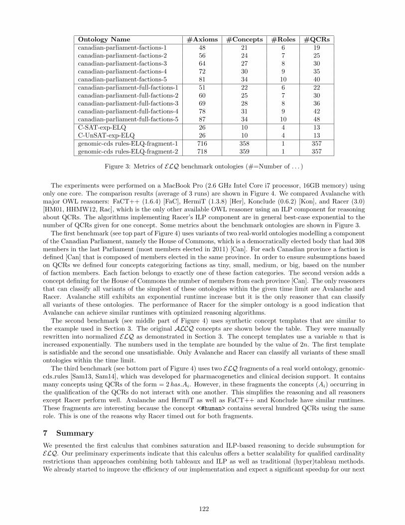
Ontology Name #Axioms #Concepts #Roles #QCRscanadian-parliament-factions-1 48 21 6 19canadian-parliament-factions-2 56 24 7 25canadian-parliament-factions-3 64 27 8 30canadian-parliament-factions-4 72 30 9 35canadian-parliament-factions-5 81 34 10 40canadian-parliament-full-factions-1 51 22 6 22canadian-parliament-full-factions-2 60 25 7 30canadian-parliament-full-factions-3 69 28 8 36canadian-parliament-full-factions-4 78 31 9 42canadian-parliament-full-factions-5 87 34 10 48C-SAT-exp-ELQ 26 10 4 13C-UnSAT-exp-ELQ 26 10 4 13genomic-cds rules-ELQ-fragment-1 716 358 1 357genomic-cds rules-ELQ-fragment-2 718 359 1 357

Figure 3: Metrics of ELQ benchmark ontologies (#=Number of . . . )

The experiments were performed on a MacBook Pro (2.6 GHz Intel Core i7 processor, 16GB memory) usingonly one core. The comparison results (average of 3 runs) are shown in Figure 4. We compared Avalanche withmajor OWL reasoners: FaCT++ (1.6.4) [FaC], HermiT (1.3.8) [Her], Konclude (0.6.2) [Kon], and Racer (3.0)[HM01, HHMW12, Rac], which is the only other available OWL reasoner using an ILP component for reasoningabout QCRs. The algorithms implementing Racer’s ILP component are in general best-case exponential to thenumber of QCRs given for one concept. Some metrics about the benchmark ontologies are shown in Figure 3.

The first benchmark (see top part of Figure 4) uses variants of two real-world ontologies modelling a componentof the Canadian Parliament, namely the House of Commons, which is a democratically elected body that had 308members in the last Parliament (most members elected in 2011) [Can]. For each Canadian province a faction isdefined [Can] that is composed of members elected in the same province. In order to ensure subsumptions basedon QCRs we defined four concepts categorizing factions as tiny, small, medium, or big, based on the numberof faction members. Each faction belongs to exactly one of these faction categories. The second version adds aconcept defining for the House of Commons the number of members from each province [Can]. The only reasonersthat can classify all variants of the simplest of these ontologies within the given time limit are Avalanche andRacer. Avalanche still exhibits an exponential runtime increase but it is the only reasoner that can classifyall variants of these ontologies. The performance of Racer for the simpler ontology is a good indication thatAvalanche can achieve similar runtimes with optimized reasoning algorithms.

The second benchmark (see middle part of Figure 4) uses synthetic concept templates that are similar tothe example used in Section 3. The original ALCQ concepts are shown below the table. They were manuallyrewritten into normalized ELQ as demonstrated in Section 3. The concept templates use a variable n that isincreased exponentially. The numbers used in the template are bounded by the value of 2n. The first templateis satisfiable and the second one unsatisfiable. Only Avalanche and Racer can classify all variants of these smallontologies within the time limit.

The third benchmark (see bottom part of Figure 4) uses two ELQ fragments of a real world ontology, genomic-cds rules [Sam13, Sam14], which was developed for pharmacogenetics and clinical decision support. It containsmany concepts using QCRs of the form = 2 has.Ai. However, in these fragments the concepts (Ai) occurring inthe qualification of the QCRs do not interact with one another. This simplifies the reasoning and all reasonersexcept Racer perform well. Avalanche and HermiT as well as FaCT++ and Konclude have similar runtimes.These fragments are interesting because the concept <#human> contains several hundred QCRs using the samerole. This is one of the reasons why Racer timed out for both fragments.

7 Summary

We presented the first calculus that combines saturation and ILP-based reasoning to decide subsumption forELQ. Our preliminary experiments indicate that this calculus offers a better scalability for qualified cardinalityrestrictions than approaches combining both tableaux and ILP as well as traditional (hyper)tableau methods.We already started to improve the efficiency of our implementation and expect a significant speedup for our next

122

Canadian Parliament Factions only Canadian Parliament Full#F Ava Fac Her Kon Rac Ava Fac Her Kon Rac

5 11.1 TO TO TO 0.12 375 TO TO TO TO4 8.4 TO TO TO 0.11 22.4 TO TO TO TO3 2.7 TO TO TO 0.07 4.1 TO TO TO TO2 1.4 TO TO TO 0.07 2.7 TO TO TO 10.51 0.8 TO TO 7.3 0.05 1.1 TO TO TO 0.44

C-SAT-exp-ELQ C-UnSAT-exp-ELQn Ava Fac Her Kon Rac Ava Fac Her Kon Rac40 0.69 TO TO TO 0.01 0.63 TO TO TO 0.0120 0.62 TO TO TO 0.01 0.80 TO TO TO 0.0110 0.63 TO TO TO 0.01 0.99 TO TO TO 0.015 0.72 6.3 4.4 0.91 0.01 0.74 TO TO 784 0.013 0.62 0.17 0.18 0.33 0.01 0.75 0.25 1.15 1.18 0.01

Sat: C v (≤ nR.¬A t ≤ n−1R.¬B) u ≥ 2nR.> u≤ nR.A u ≤ nR.BUnsat: C v (≤ n−1R.¬At≤ n−1R.¬B)u≥ 2nR.>u≤ nR.Au≤ nR.B

Satisfiability of concept <#human>

Name Ava Fac Her Kon Racgenomic-cds rules-ELQ-fragment-1 1.13 27.7 0.87 27.7 TOgenomic-cds rules-ELQ-fragment-2 2.4 28.2 1.14 28.3 TO

Figure 4: Benchmark runtimes in seconds with a timeout of 1000 seconds (TO=timeout, #F=Number of Factions,Ava=Avalanche, Fac=FaCT++, Her=HermiT, Kon=Konclude, Rac=Racer)

release. We plan to add a preprocessing phase that automatically rewrites ALCQ ontologies to our ELQ syntax.Our next steps are to extend our calculus to cover role hierarchies and inverse roles.

References

[ADF09] H. M. B. Amor, J. Desrosiers, and A. Frangioni. On the choice of explicit stabilizing terms in columngeneration. Discrete Applied Mathematics, 157(6):1167–1184, 2009.

[BBL05] F. Baader, S. Brandt, and C. Lutz. Pushing the EL envelope. In Proc. of IJCAI, pages 364–369,2005.

[BJN+98] C. Barnhart, E. L. Johnson, G. L. Nemhauser, M. W. P. Savelsbergh, and P. H. Vance. Branch-and-price: Column generation for solving huge integer programs. Operations Research, 46(3):316–329,1998.

[BMC+16] A. Bate, B. Motik, B. Cuenca Grau, F. Simancık, and I. Horrocks. Extending consequence-basedreasoning to SRIQ. In Proc. of KR, pages 187–196, 2016.

[Can] Canadian Parliament. https://en.wikipedia.org/wiki/House of Commons of Canada.

[Chv83] V. Chvatal. Linear Programming. Freeman, 1983.

[DDS11] G. Desaulniers, J. Desrosiers, and S. Spoorendonk. Cutting planes for branch-and-price algorithms.Networks, 58:301–310, 2011.

[DGL14] J. Desrosiers, J. Gauthier, and M. Lubbecke. Row-reduced column generation for degenerate masterproblems. European Journal of Operational Research, 236:453–460, July 2014.

[DW60] G. B. Dantzig and P. Wolfe. Decomposition principle for linear programs. Operations research,8(1):101–111, 1960.

[FaC] FaCT++. http://owl.cs.manchester.ac.uk/tools/fact/.

123

[FH10a] J. Faddoul and V. Haarslev. Algebraic tableau reasoning for the description logic SHOQ. Journalof Applied Logic, 8(4):334–355, 2010.

[FH10b] J. Faddoul and V. Haarslev. Optimizing algebraic tableau reasoning for SHOQ: First experimentalresults. In Proc. of DL, pages 161–172, 2010.

[FH10c] N. Farsiniamarj and V. Haarslev. Practical reasoning with qualified number restrictions: A hybridAbox calculus for the description logic SHQ. AI Communications, 23(2-3):334–355, 2010.

[GG61] P. C. Gilmore and R. E. Gomory. A linear programming approach to the cutting-stock problem.Operations research, 9(6):849–859, 1961.

[HB91] B. Hollunder and F. Baader. Qualifying number restrictions in concept languages. In Proc. of KR,pages 335–346, 1991.

[Her] HermiT. http://www.hermit-reasoner.com/download.html.

[HHMW12] V. Haarslev, K. Hidde, R. Moller, and M. Wessel. The RacerPro knowledge representation andreasoning system. Semantic Web, 3(3):267–277, 2012.

[HM01] V. Haarslev and R. Moller. RACER system description. In Proc. of IJCAR, pages 701–705, 2001.

[IBM] IBM. https://www.ibm.com/developerworks/downloads/ws/ilogcplex/.

[Kaz09] Y. Kazakov. Consequence-driven reasoning for horn SHIQ ontologies. In Proc. of IJCAI, pages2040–2045, 2009.

[Kon] Konclude. http://www.derivo.de/en/produkte/konclude/.

[Las70] L. Lasdon. Optimization Theory for Large Systems. MacMillan, New York, 1970.

[LD05] M. Lubbecke and J. Desrosiers. Selected topics in column generation. Operations Research, 53:1007–1023, 2005.

[Meg87] N. Megiddo. On the complexity of linear programming. In Advances in Economic Theory, pages225–268. Cambridge University Press, 1987.

[NW88] G. L. Nemhauser and L. A. Wolsey. Integer and Combinatorial Optimization. Wiley, New York,1988.

[NW99] G. Nemhauser and L. Wolsey. Integer and Combinatorial Optimization. Wiley, 1999. reprint of the1988 edition.

[OK99] H. Ohlbach and J. Kohler. Modal logics, description logics and arithmetic reasoning. ArtificialIntelligence, 109(1-2):1–31, 1999.

[Rac] Racer. https://www.ifis.uni-luebeck.de/index.php?id=385.

[RH12] L. Roosta Pour and V. Haarslev. Algebraic reasoning for SHIQ. In Proc. of DL, pages 530–540,2012.

[Sam13] M. Samwald. Genomic CDS: an example of a complex ontology for pharmacogenetics and clinicaldecision support. In 2nd OWL Reasoner Evaluation Workshop, pages 128–133. CEUR, 2013.

[Sam14] M. Samwald. An update on genomic CDS, a complex ontology for pharmacogenomics and clinicaldecision support. In 3rd OWL Reasoner Evaluation Workshop, pages 58–63. CEUR, 2014.

[SGL14] A. Steigmiller, B. Glimm, and T. Liebig. Coupling tableau algorithms for expressive descriptionlogics with completion-based saturation procedures. In Proc. of IJCAR, pages 449–463, 2014.

[SMH14] F. Simancık, B. Motik, and I. Horrocks. Consequence-based and fixed-parameter tractable reasoningin description logics. Artificial Intelligence, 209:29–77, 2014.

[Van11] F. Vanderbeck. Branching in branch-and-price: a generic scheme. Mathematical Programming,130(2):249–294, 2011.

124

The PIE Environment for First-Order-Based

Proving, Interpolating and Eliminating

Christoph Wernhard

TU Dresden, Dresden, Germany

Abstract

The PIE system aims at providing an environment for creating com-plex applications of automated first-order theorem proving techniques.It is embedded in Prolog. Beyond actual proving tasks, also interpo-lation and second-order quantifier elimination are supported. A macrofeature and a LATEX formula pretty-printer facilitate the construction ofelaborate formalizations from small, understandable and documentedunits. For use with interpolation and elimination, preprocessing opera-tions allow to preserve the semantics of chosen predicates. The systemcomes with a built-in default prover that can compute interpolants.

1 Introduction

The PIE system aims at providing an environment for creating complex applications of automated first-ordertheorem proving techniques, in examples, experiments, benchmarks, and as background machinery in othercontexts. The system is currently under development, with some major components already functional butothers still on the agenda. The state of the art for practically applying first-order proving techniques is perhapsbest represented by the the TPTP [Sut09, Sut15], which – although designed primarily as a library for testingtheorem provers – supports some aspects of creating complex applications: the Prolog-readable TPTP formulasyntax provides a uniform interface to a variety of systems, proving problems are organized in a way thatfacilitates repeatability of testing, utilities for preprocessing are provided, and the classification of problemsaccording to useful syntactic characteristics is supported. When creating complex applications becomes themain focus, various further issues arise:

1. Tasks beyond Proving. Aside of theorem proving in the literal sense there are various other related taskswhich share techniques with first-order theorem proving and have interesting applications. Basic such tasksare model computation, which became popular in knowledge representation as answer set programming, thecomputation of first-order interpolants and second-order quantifier elimination.

From a certain point of view, the opening of first-order reasoning to second-order extensions seemsquite natural: Early technical investigations of first-order logic have been accompanied by investigations ofsecond-order quantifier elimination for formulas with just unary predicates [Lo15, Sko19, Beh22] (see [Cra08];for a comprehensive presentation of [Beh22] in this context see [Wer15a]). Today there are many knownapplications of second-order quantifier elimination and variants of it termed uniform interpolation, forgettingand projection. Aside of the study of modal logics, most of these applications are in knowledge representationand include computation of circumscription, representation of nonmonotonic semantics, abduction with

Copyright c© by the paper’s authors. Copying permitted for private and academic purposes.

In: P. Fontaine, S. Schulz, J. Urban (eds.): Proceedings of the 5th Workshop on Practical Aspects of Automated Reasoning(PAAR 2016), Coimbra, Portugal, 02-07-2016, published at http://ceur-ws.org

125

respect to such semantics, forgetting in knowledge bases, and approaches to modularization of knowledgebases based on the notion of conservative extension, e.g., [GO92, LR94, D LS97, Wer04, GLW06, GSS08,GHKS08, LW11, Wer12, Wer13a, KS13, LK14]. Advanced elimination systems are available for descriptionlogics, for example the LETHE system [KS15] as well as further implementations of recent techniques forforgetting based on Ackermann’s lemma [ZS15, ZS16]. Elimination systems based on first-order logic havebeen implemented mainly in the late 1990s [Eng96, Gus96].

Interpolation plays an important role in verification [McM05], where it is used mainly on the basis ofpropositional logic extended with respect to specific theories. An application area on the basis of full first-order logic is database query rewriting [Mar07, NSV10, TW11, BBtC13, BtCT14, HTW15]. It seems thatso far there have been only specialized techniques applied in this context, in contrast to general first-orderprovers. Interpolation for first-order logic is supported by Princess [BKRW11b, BKRW11a], as well as insome versions/extensions of Vampire [HKV10, HHKV12].

2. First-Order Logic as Input and Presentation Format. First-order logic can be considered as closeenough to natural language to be well suited for humans to express applications. (This is quite differentfrom propositional logic, where the formulas input to SAT solvers are typically the output of some encodingmechanism of the application problem. Accordingly, in the DIMACS format commonly used as input for SATsolvers logic atoms are just represented by natural numbers.) Compared to Prolog notation, readability offirst-order formulas can in some cases be improved if functor arguments are not encapsulated by parenthesesand not separated by commas, which however requires predeclaration of functor arities. The textbook[EFT84], for example, would write pfxy instead of p(f(x), y). Pretty-printing, where formula structure isreflected in indentation substantially facilitates readability of longer formulas. LATEX provides professionalformula layout and seems the format of choice for the presentation of formalizations.

The TPTP syntax allows formulas to be read in by Prolog systems, which is very convenient for Prologimplementations of further formula manipulation. The TPTP tools also include a pretty-printer for thatsyntax. There are two subtle mismatches of the TPTP syntax and Prolog: TPTP formula variables arerepresented as Prolog variables, although their scoping is different (quantifier arguments vs. clauses); inthe ISO Prolog standard unfortunately the character ! is, unlike ?, not of type “graphic”, effecting thatuniversal and existential TPTP quantifier symbols, which are based on ! and ?, can not be handled inexact analogy, and that a != b has to be read in as =(!(a),b).

3. Stepwise Construction of Larger Formalizations. Comprehensibility of even modest-sized formal-izations can be improved greatly by using labels, speaking names, for the involved subformulas. In analogyto procedure names, labels are particularly versatile if they can be used with parameters. Such labels alsofacilitate the re-use of formulas and indicate similarities of related formalizations.

The TPTP requires symbolic names as formula identifiers whose scope is the respective proving problem.They typically appear in proof presentations but are not used to specify the composition of problems fromformulas. Shared axiom sets can be expressed in the TPTP by means on an include directive on the filelevel.

4. Flexibility of Document Granularity. Each proving problem in the TPTP is represented by a file whosename is formed according to a pattern such that application domain and problem format are indicated. Whilethis is very helpful for an archive and testing library, for the development of formalizations it seems morebeneficial to follow the traditional approach of the AI programming languages like Lisp and Prolog, whichdo not tie document granularity – files – with semantic or abstract structural units. However, support fornamespaces and symbol redefinition is in such language systems commonly related to files.

5. Integration of Natural Language Text. In many cases it is useful to accompany formalizations withexplanatory text. Possibly an interleaved combination of formal and informal material, a form of “literateformalizing”, is most adequate for complex formalizations.

TPTP problem files have a structured header that includes an obligatory field for an English one-linedescription as well as an optional field for a longer description. Also a field for bibliographical references isprovided.

6. Sustainability and Repeatability. The usability of documents with complex formalizations should notbe limited to a narrow context. Involved mechanized tasks must be repeatable. That a proving problem

126

can be solved not just depends on the choice of the proving system but also on its particular configuration,prone to fail after small changes. This implies that system configurations known to work have to be preciselyrecorded.

7. Benchmarks as Side Product. For the computational tasks involved in a complex formalization, itshould be possible to generate benchmark documents that can be evaluated independently and in repro-ducible ways, for example as TPTP problems files.

8. Programming Language Embedding. Embedding in a programming language seems useful: Pro-gramming is required to express advanced formula manipulations, including preprocessing or generation offormulas according to repeatedly occurring patterns and to specify flows of control concerning the involvedproving and related tasks, as well as postprocessing of their outputs. Prolog, the original basis of the TPTP,seems well suited, in particular since it supports terms as readable and printable data structures that can beimmediately used to represent logic formulas. In addition, specifically the SWI Prolog system comes withvery good interfaces to XML and RDF, which are common as exchange formats for large fact bases.

9. Integration of Large Axiom Sets and Fact Bases. Some applications, in particular in common sensereasoning, include large sets of axioms, such as, for example, the excerpts of CYC included in the TPTP, orfact bases such as YAGO, DBPedia and GND, which are available in RDF format. Naming of axioms/factsis irrelevant for these. A human user typically sees only a small fraction of them that is exposed in a proof.

TPTP v6.3.0 includes five subsets of CYC ranging form 100 up to more than 3 million axioms, whereonly the second smallest with 8000 axioms was used in the 2015 CASC-25. Seemingly that is the onethat can be handled without any special mechanisms by most modern first-order provers. With LTB theCASC also provides a dedicated division for problems with large shared axiom sets, currently extracted fromlibraries formalized with interactive proving systems. In the competition, provers are allowed to performoffline tuning with the shared axioms and example problems.

These issues are addressed by the PIE system with the features and components described in Sect. 2. In theconclusion, Sect. 3, some related work is briefly discussed and an outlook is given. An example that illustratesthe use of PIE is provided as Appendix A. Development snapshots of the system with some further examplescan be obtained under GNU General Public License from

http://cs.christophwernhard.com/pie/.

2 Features and Components of the PIE System

2.1 Prolog Embedding and Interfaces to Other Systems

The PIE system is the succesor of ToyElim [Wer13b], which is based on propositional logic and has been usedin experiments with applications of second-order operator elimination, such as forgetting, abduction and non-monotonic reasoning semantics. Both systems are implemented in SWI Prolog. To cope with large formulas, onoccasion destructive operations like setarg are used but hidden behind an hash table interface.

It is intended to use PIE from the SWI Prolog environment. Thus, the functionality of the system is providedessentially in form of a library of Prolog predicates. The basic formula syntax of PIE differs from the TPTPsyntax (see also Sect. 1, point 2): A formula with quantifiers is represented by a Prolog ground term. Forconjunction and disjunction the operators , and ;, as in Prolog, are used. Implication is represented by ->

(unfortunately this operator has due to its role as “if-then-else” in Prolog a stronger default precedence than ;).A clausal formula is represented as list of lists of literals, where variables are Prolog variables. Conversions to andfrom TPTP first-order and clausal forms as well as Otter/Prover9/Mace4 syntax are provided. For propositionallogic and quantified Boolean formulas there are conversions to and from DIMACS and QDIMACS, respectively.Call-interfaces for proving tasks to provers accepting the TPTP or the Prover9 format as well as to SAT andQBF solvers are provided. For propositional elimination tasks there is also a special DIMACS -based interfaceto Coprocessor [Man12], a SAT preprocessor that can be configured to perform elimination tasks.

The PIE system includes the Prolog-based first-order prover CM, described further in Sect. 2.4, which is thusimmediately available in a lightweight way, without detour through the operation system and without furtherinstallation effort. Proofs returned by CM can be directly processed with Prolog and allow interpolant extraction.The internals of the prover are easy to modify for experimenting. As a second possibility for interpolation tasks,an interface to Princess [BKRW11b] is envisaged.

127

2.2 Macros

A macro facility is provided, where the macros can have parameters and expand to first- or second-order formulas.In this way, a macro name can serve not just as a formula label but, more generally, can be used within anotherformula in subformula position, possibly with arguments.

Pattern matching is used to choose the effective declaration for expansion, allowing structural recursion inmacro declarations. An optional Prolog body in a macro declaration permits expansions involving arbitrarycomputations. Utility predicates intended for use in these bodies are provided for common tasks, for example,determining the predicates in a formula after expansion. With a macro declaration, properties of its lexicalenvironment, in particular configuration settings that affect the expansion, are recorded.

Macros provide a convenient way to express properties of predicates, e.g., transitivity, abstractly, and also toexpress more complex application patterns that can not be stated as definitions within second-order logic unlesspredicates in argument position would be permitted. Various practically useful computations can be consideredas elimination of second-order operators, in particular, literal forgetting (a form of predicate quantificationthat only affects predicate occurrences with negative or positive polarity), projection (which is like predicatequantification, except that the predicates that are not quantified – whose semantics is to be retained – are madeexplicit) and circumscription. The macro mechanism allows to use dedicated operator notation for these on theuser level, whereas on the system level predicate quantification is the only second-order operator that needs tobe supported.

2.3 LATEX Document Generation

A formula pretty-printer is available that outputs Prolog-readable syntax as well as LATEX. In addition to formulaindentation, the LATEX pretty-printer converts numbers and single characters separated by an underscore at theend of Prolog functor names to subscripts in LATEX. A brief syntax as indicated in Sect. 1, point 2, is optionallyavailable for in- and output of formulas.

Prolog-readable files with macro declarations can be translated to LATEX documents which contain the pretty-printed declarations, all text within specially marked comments, and all outputs produced by calls wrapped ina special Prolog predicate that indicates evaluation at “printtime”. Utility predicates for tasks like proving,interpolation and elimination are provided that pretty-print solutions in LATEX at “printtime”, and in Prologwhen invoked normally.

2.4 Included Prolog Technology Theorem Prover CM

The included prover CM was originally written in 1992, based on [Sti88] but as compiler to Prolog instead ofLisp. The underlying calculus can be understood as model elimination, as clausal tableau construction, or as theconnection method. The leanCoP prover [Ott10], also implemented in Prolog, is based on the same calculus andregularly takes part in the CASC competitions. Re-implementations of leanCoP have recently found interest tostudy new techniques [Kal15, KU15]. A conceptual difference to leanCoP is that CM proceeds in a two-stepway, by first compiling the proving problem. This makes the prover less flexible at runtime, but the possibilityto inspect the output of the compiler on its own contributes to robustness and facilitates experimenting withmodifications. The prover had been revised in 1997 [DW97] and recently in 2015 where it has been ported toSWI Prolog, combined with some newly implemented preprocessing operations and improved with the problemsof the 2015 CASC competition, CASC-25 , taken as yardstick. For the CASC-25 problems in the first-order noequality (FNE) category it performs better than leanCop and iProver Modulo but worse than CVC4. For theCASC-25 problems in the first-order with equality (FEQ) category it performs significantly worse than leanCopbut better than iProver Modulo. More information on the prover and the evaluation details are available athttp://cs.christophwernhard.com/pie/cmprover/.

2.5 Preprocessing with Semantics Preservation for Chosen Predicates

A number of implemented preprocessing operations is included, most of them currently for clausal inputs.While some of these preserve equivalence, for example conventional CNF transformation (if function introduc-tion through Skolemization is disregarded), others preserve equivalence just with respect to a set of predicatesp1, . . . pn, that is, inputs F and outputs G satisfy the second-order equivalence

∃q1 . . . ∃qm F ≡ ∃q1 . . . ∃qmG, (1)

128

where q1, . . . , qm are all involved predicates with exception of p1, . . . pn. Such conversions clearly also preserveequi-satisfiability, which corresponds just to the special case where n = 0. Keeping track of the predicatesp1, . . . , pn whose semantics is to preserve is needed for preprocessing in applications like interpolation and second-order quantifier elimination. (The Riss SAT solver and the related preprocessor Coprocessor [Man12] also supportthis.) Some preprocessing conversions allow, moreover, to keep track of predicate semantics with respect to justtheir occurrences with positive or negative polarity, which is useful for Lyndon interpolation (Sect. 2.6) andliteral forgetting (Sect. 2.2).

Implemented preprocessing methods that preserve equivalence with respect to a given set of predicates includea variant of the Plaisted-Greenbaum transformation, a structural hashing transformation that identifies twopredicates (or one predicate with the negation of another) in the case where both have equivalent non-recursiveand easily detectable “semi-definitions” (the, say, positive “semi-definition” of the predicate p is obtained bytaking all clauses containing a positive literal with predicate p and removing these literals, equivalence (4) belowcan be used to justify this transformation semantically), and elimination of predicates in cases where this doesnot lead to a substantial increase of the formula size.

2.6 Support for Interpolation

A Craig interpolant for two given first-order formulas F and G such that (F → G) is valid is a first-orderformula H such that (F → H) and (H → G) are valid and H contains only symbols (predicates, functions,constants, free variables) that occur in both F and G. Craig’s interpolation theorem ensures the existence ofsuch interpolants. The PIE system supports the computation of Craig interpolants from closed clausal tableauxwith a variant of the tableau-based interpolant construction method from [Smu95, Fit95]. (It seems that thismethod has not been reviewed in the recent literature on interpolation for first-order logic in automated systems,e.g., [HKV10, BKRW11a, BJ15].)

Suitable clausal tableaux are constructed by the CM prover. Interpolant construction can there be doneentirely by pre- and postprocessing, without requiring alterations to the core prover. The preprocessing includessimplifications as outlined in Sect. 2.5. Also the Hyper hypertableau prover [PW07] produces proof terms thatcan be converted to tableaux, but this is not fully worked out in the current implementation.

The constructed interpolants strengthen the requirements for Craig interpolants in that they are actuallyLyndon interpolants, that is, predicates occur in them only in polarities in which they occur in both of the twoinput formulas. Symmetric interpolation, a generalization of interpolation described in [Cra57, Lemma 2] andcalled symmetric, e.g., in [McM05, Sect. 5], is supported, implemented by computing a conventional interpolantfor each of the input formulas, corresponding to the induction suggested in [Cra57]. Handling of functions (withexception of individual constants) is not supported in the current implementation. It seems possible to implementthis by a relational translation of the functions that is reversed on the output.

2.7 Support for Second-Order Extensions to First-Order Logic

In some cases second-order formalizations are convertible to first-order logic but more concise than their first-ordercounterparts. This suggests to use preprocessors that produce first-order outputs to handle such second-orderinputs. The following equivalence is analogous to the familiar effect of Skolemization of individual variablesquantified by outermost quantifiers but applies to predicate variables:

∃p1 . . . ∃pn F [p1, . . . , pn] |= ∀q1 . . . ∀qmG[q1 . . . , qm] iff F [p′1, . . . , p′n] |= G[q′1 . . . , q

′m], (2)

where F [p′1, . . . , p′n] is obtained from F [p1, . . . , pn] by replacing all occurrences of predicates pi for 1 ≤ i ≤ n with

fresh predicates p′i and, analogously, G[q′1 . . . , q′m] from G[q1 . . . , qm] by replacing qi for 1 ≤ i ≤ m with fresh q′i.

The left side of (2) is a second-order entailment, the right side a first-order entailment. This pattern occurs in thecharacterization of definability and computation of definientia by interpolation (see Appendix A for an example),where advantages of the second-order formulation are that predicate renaming is hidden by quantification andthat a relation to the strongest necessary and weakest sufficient condition [Lin01, D LS01, Wer12], which areessentially second-order concepts, is made explicit.

Moving second-order quantifiers outward can be necessary to achieve a form matching the left side of (2).Aside of the equivalence preserving quantifier movement operations familiar from first-order quantifiers, thefollowing second-order equivalence, “Ackermann’s quantifier switching”, due to [Ack35b] can be useful there:

∀x∃pF [pt1, . . . , ptm] ≡ ∃q∀xF [qxt1, . . . , qxtm], (3)

129

where F [pt1, . . . , ptm] is a second-order formula in which x only occurs free and p is a predicate of arity n ≥ 0 withexactly the m indicated occurrences, instantiated with n-ary argument sequences t1 to tm and F [qxt1, . . . , qxtm]is like F [pt1, . . . , ptm] except that the occurrences of p are replaced by occurrences of a fresh predicate q ofarity n + 1, applied on the original argument sequences ti prepended by x. Applied in the converse directionthan displayed here, the equivalence (3) can help to facilitate second-order quantifier elimination by simplifyingthe argument formula of the predicate quantifier, leading for example to an elimination-based decision methodfor the description logic ALC [Wer15b]. The current implementation of PIE includes automatic handling ofsecond-order quantifiers in proving tasks according to (2). More advanced preprocessing is planned.

2.8 Support for Second-Order Quantifier Elimination

Second-order quantifier elimination means to compute for a given formula with second-order quantifiers, that is,quantifiers upon predicate or function symbols, an equivalent first-order formula. (For functions an arity > 0,in contrast to individual constants, is assumed here.)

For Boolean quantifier elimination, that is, second-order quantifier elimination on the basis of propositionallogic, several methods were already available in the ToyElim system: expanding subformulas with the Shannonexpansion followed by simplifications (a more advanced version of this method is described in [Wer09]), andfor clausal formulas a resolution-based method as well and a call-interface to Coprocessor [Man12], a SATpreprocessor that can be configured to perform resolution-based elimination. For first-order logic, the PIEsystem currently includes a variant of the DLS algorithm [D LS97], which is based on Ackermann’s Lemma, thefollowing equivalence due to [Ack35a]:

∃p (∀x px→ G[x]) ∧ F [pt1, . . . , ptn] ≡ F [G[t1], . . . , G[tn]], (4)

where p does not occur in G[x] and does occur in F in exactly the n indicated occurrences which all havepositive polarity, and F [G[t1], . . . , G[tn]] is obtained from F [pt1, . . . , ptn] by replacing all occurrences of p withoccurrences of G[x] in which x is instantiated to the respective argument ti of p. (It is assumed that x does notoccur bound in G[x].) The lemma obviously also holds in a dual version, where the implication is (∀x px← G[x])and the occurences in F all have negative polarity. It can be straightforwardly generalized to predicates p withmore than a single argument.

The improvement of the second-order quantifier elimination techniques and their integration with the othersupported tasks belong to the major issues for the next development steps.

3 Conclusion

Concerning related work based on first-order proving, the TPTP had already been mentioned in many specificcontexts. For developing certain kinds of advanced and complex mathematical proofs in a human-assisted way,some first-order systems, notably Otter and Prover9/Mace4, alone seem suitable by providing control featuressuch as weighting and hints. The most ambitious approach for a working environment around first-order proversso far seemed to be the ILF project in the 1990s, targeted at human users and mathematical applications. Itwas centered around an advanced proof conversion with LATEX presentation in textbook style [DGH+94, Dah98].Further goals were a mathematical library based on Mizar and an embedding into the Mathematica environment[DW97, DHHW98]. The goals of PIE are much more modest. The main focus is not on proofs but on formulas,possibly reduced by elimination and normalized in certain ways. In the conception of the ILF MathematicalLibrary there was a somewhat ad hoc pragmatic break between syntactic preselection of possibly relevant axiomsand their semantic processing by provers. It is the hope that second-order techniques justify a more thoroughlysemantic approach to modularization and retrieval from formalized knowledge bases.

It is planned to use PIE embedded into another Prolog-based system that provides knowledge based supportfor scholarly editing [KW16a, KW16b]. The first envisaged application there is to control the preprocessing ofRDF fact bases through definienda obtained by interpolation.

As already indicated in Sect. 2.8, the extension of the facilities for second-order quantifier elimination willbe a main issue for the next development steps of PIE . Aside of DLS, the second major approach to second-order quantifier elimination is the resolution-based SCAN algorithm. A variant of this has also been alreadyimplemented in PIE but mainly for abstract investigations, without expectation to compete with possible im-plementations based on dedicated resolution provers. DLS is known to be complete (i.e. terminate successfully)exactly for inputs that satisfy a certain syntactic condition [Con06]. Orthogonal to that condition, there are

130

further cases with known terminating methods, for example, formulas with only unary predicates [Lo15, Beh22](see also [Wer15b]), “semi-monadic” formulas [Wer15b], and the case where explicitly given ground atoms are“forgotten” [LR94]. Various elimination techniques have thus to be combined for practical application, in a waythat ensures completeness for known cases.

A related topic for future research is the exploration of relationships between interpolation and elimination.For example, the objective of one of the preprocessing steps of DLS is to decompose a given formula into aconjunction A ∧ B where A contains the predicate p to eliminate just in occurrences with negative polarityand B just with positive polarity, approximately matching the conjunction in the left side of (4). Symmetricinterpolation can be used to solve this step in a complete way, that is, whenever there is a decomposition intosuch A and B, then one is found. Other parallels between interpolation and elimination concern the notion ofconservative extension, a relationship between formulas that can be expressed as entailment of an existentialsecond-order formula. For the special case of definitional extension (see e.g., [Hod97]), also if the extension isnot given in the syntactic form of explicit definitions, the corresponding task can be expressed by first-orderreasoning based on interpolation.

To sum up, the PIE system tries to supplement what is needed to create applications with techniques ofautomated first-order proving techniques, not solely in the sense of mathematical theorem proving but consideredas general tools of information processing. The main focus are formulas, as constituents of complex formalizationsand as results of elimination and interpolation. Special emphasis is made on utilizing some natural relationshipsbetween first- and second-order logics. Key ingredients of the system are macros, LATEX prettyprinting andintegration into a programming environment.

Acknowledgments

This work was supported by DFG grant WE 5641/1-1.

References

[Ack35a] Wilhelm Ackermann. Untersuchungen uber das Eliminationsproblem der mathematischen Logik.Mathematische Annalen, 110:390–413, 1935.

[Ack35b] Wilhelm Ackermann. Zum Eliminationsproblem der mathematischen Logik. Mathematische Anna-len, 111:61–63, 1935.

[BBtC13] Vince Barany, Michael Benedikt, and Balder ten Cate. Rewriting guarded negation queries. InMFCS 2013, volume 8087 of LNCS, pages 98–110. Springer, 2013.

[Beh22] Heinrich Behmann. Beitrage zur Algebra der Logik, insbesondere zum Entscheidungsproblem. Ma-thematische Annalen, 86(3–4):163–229, 1922.

[BJ15] Maria Paola Bonacina and Moa Johansson. Interpolation systems for ground proofs in automateddeduction: a survey. Journal of Automated Reasoning, 54(4):353–390, 2015.

[BKRW11a] Angelo Brillout, Daniel Kroening, Philipp Rummer, and Thomas Wahl. Beyond quantifier-freeinterpolation in extensions of Presburger arithmetic. In VMCAI 2011, volume 6538 of LNCS, pages88–102. Springer, 2011.

[BKRW11b] Angelo Brillout, Daniel Kroening, Philipp Rummer, and Thomas Wahl. An interpolating sequentcalculus for quantifier-free Presburger arithmetic. Journal of Automated Reasoning, 47(4):341–367,2011.

[BtCT14] Michael Benedikt, Balder ten Cate, and Efthymia Tsamoura. Generating low-cost plans from proofs.In PODS’14, pages 200–211. ACM, 2014.

[Con06] Willem Conradie. On the strength and scope of DLS. Journal of Applied Non-Classsical Logics,16(3–4):279–296, 2006.

[Cra57] William Craig. Three uses of the Herbrand-Gentzen theorem in relating model theory and prooftheory. Journal of Symbolic Logic, 22(3):269–285, 1957.

[Cra08] William Craig. Elimination problems in logic: A brief history. Synthese, (164):321–332, 2008.

[Dah98] Bernd Ingo Dahn. Robbins algebras are Boolean: A revision of McCune’s computer-generatedsolution of Robbins problem. Journal of Algebra, 208(2):526–532, 1998.

[DGH+94] Bernd Ingo Dahn, Jurgen Gehne, Thomas Honigmann, Lutz Walther, and Andreas Wolf. Integrat-ing logical functions with ILF. Technical Report Preprints aus dem Institut fur Mathematik 10,Humboldt Universitat zu Berlin, Institut fur Mathematik, 1994.

131

[DHHW98] Bernd Ingo Dahn, Andreas Haida, Thomas Honigmann, and Christoph Wernhard. Using Mathe-matica and automated theorem provers to access a mathematical library. In CADE-15 Workshopon Integration of Deductive Systems, pages 36–43, 1998.

[D LS97] Patrick Doherty, Witold Lukaszewicz, and Andrzej Sza las. Computing circumscription revisited: Areduction algorithm. Journal of Automated Reasoning, 18(3):297–338, 1997.

[D LS01] Patrick Doherty, Witold Lukaszewicz, and Andrzej Sza las. Computing strongest necessary andweakest sufficient conditions of first-order formulas. In IJCAI-01, pages 145–151. Morgan Kauf-mann, 2001.

[DW97] Ingo Dahn and Christoph Wernhard. First order proof problems extracted from an article in theMizar mathematical library. In FTP’97, RISC-Linz Report Series No. 97–50, pages 58–62. JohannesKepler Universitat, Linz, 1997.

[EFT84] Heinz-Dieter Ebbinghaus, Jorg Flum, and Wolfgang Thomas. Mathematical Logic. Springer, 1984.

[Eng96] Thorsten Engel. Quantifier elimination in second-order predicate logic. Master’s thesis, Max-Planck-Institut fur Informatik, Saarbrucken, 1996.

[Fit95] Melvin Fitting. First-Order Logic and Automated Theorem Proving. Springer, 2nd edition, 1995.

[GHKS08] Bernardo Cuenca Grau, Ian Horrocks, Yevgeny Kazakov, and Ulrike Sattler. Modular reuse ofontologies: Theory and practice. Journal of Artificial Intelligence Research, 31(1):273–318, 2008.

[GLW06] Silvio Ghilardi, Carsten Lutz, and Frank Wolter. Did I damage my ontology? A case for conservativeextensions in description logics. In KR 06, pages 187–197. AAAI Press, 2006.

[GO92] Dov Gabbay and Hans Jurgen Ohlbach. Quantifier elimination in second-order predicate logic. InKR’92, pages 425–435. Morgan Kaufmann, 1992.

[GSS08] Dov M. Gabbay, Renate A. Schmidt, and Andrzej Sza las. Second-Order Quantifier Elimination:Foundations, Computational Aspects and Applications. College Publications, 2008.

[Gus96] Joakim Gustafsson. An implementation and optimization of an algorithm for reducing formulae insecond-order logic. Technical Report LiTH-MAT-R-96-04, Univ. Linkoping, 1996.

[HHKV12] Krystof Hoder, Andreas Holzer, Laura Kovacs, and Andrei Voronkov. Vinter: A Vampire-basedtool for interpolation. In APLAS 2012, volume 7705 of LNCS, pages 148–156. Springer, 2012.

[HKV10] Krystof Hoder, Laura Kovacs, and Andrei Voronkov. Interpolation and symbol elimination inVampire. In IJCAR 2010, volume 6173 of LNCS, pages 188–195. Springer, 2010.

[Hod97] Wilfrid Hodges. A Shorter Model Theory. Cambridge University Press, Cambridge, 1997.

[HTW15] Alexander Hudek, David Toman, and Grant Wedell. On enumerating query plans using analytictableau. In TABLEAUX 2015, volume 9323 of LNCS (LNAI), pages 339–354. Springer, 2015.

[Kal15] Cezary Kaliszyk. Efficient low-level connection tableaux. In TABLEAUX 2015, volume 9323 ofLNCS (LNAI), pages 102–111. Springer, 2015.

[KS13] Patrick Koopmann and Renate A. Schmidt. Uniform interpolation of ALC-ontologies using fix-points. In FroCoS 2013, volume 8152 of LNCS (LNAI), pages 87–102. Springer, 2013.

[KS15] Patrick Koopmann and Renate Schmidt. LETHE: Saturation-based reasoning for non-standardreasoning tasks. In ORE 2015. CEUR-WS.org, 2015.

[KU15] Cezary Kaliszyk and Josef Urban. FEMaLeCoP: Fairly efficient machine learning connection prover.In LPAR-20, volume 9450 of LNCS, pages 88–96. Springer, 2015.

[KW16a] Jana Kittelmann and Christoph Wernhard. Knowledge-based support for scholarly editing and textprocessing. In DHd 2016 – Konferenzabstracts, pages 176–179. nisaba verlag, 2016.

[KW16b] Jana Kittelmann and Christoph Wernhard. Towards knowledge-based assistance for scholarly edit-ing. In AITP 2016 (Book of Abstracts), 2016.

[Lin01] Fangzhen Lin. On strongest necessary and weakest sufficient conditions. Artificial Intelligence,128:143–159, 2001.

[LK14] Michel Ludwig and Boris Konev. Practical uniform interpolation and forgetting for ALC TBoxeswith applications to logical difference. In KR’14. AAAI Press, 2014.

[LR94] Fangzhen Lin and Raymond Reiter. Forget It! In Working Notes, AAAI Fall Symp. on Relevance,pages 154–159, 1994.

[LW11] Carsten Lutz and Frank Wolter. Foundations for uniform interpolation and forgetting in expressivedescription logics. In IJCAI-11, pages 989–995. AAAI Press, 2011.

[Lo15] Leopold Lowenheim. Uber Moglichkeiten im Relativkalkul. Mathematische Annalen, 76:447–470,1915.

132

[Man12] Norbert Manthey. Coprocessor 2.0 – a flexible CNF simplifier. In SAT ’12, volume 7317 of LNCS,pages 436–441. Springer, 2012.

[Mar07] Maarten Marx. Queries determined by views: Pack your views. In PODS ’07, pages 23–30. ACM,2007.

[McM05] Kenneth L. McMillan. Applications of Craig interpolants in model checking. In TACAS 2005,volume 3440 of LNCS, pages 1–12, Berlin, Heidelberg, 2005. Springer.

[NSV10] Alan Nash, Luc Segoufin, and Victor Vianu. Views and queries: Determinacy and rewriting. ACMTransactions on Database Systems, 35(3), 2010.

[Ott10] Jens Otten. Restricting backtracking in connection calculi. AI Communications, 23(2-3):159–182,2010.

[PW07] Bjorn Pelzer and Christoph Wernhard. System description: E-KRHyper. In CADE-21, volume4603 of LNCS (LNAI), pages 503–513. Springer, 2007.

[Sko19] Thoralf Skolem. Untersuchungen uber die Axiome des Klassenkalkuls und uber Produktations-und Summationsprobleme welche gewisse Klassen von Aussagen betreffen. VidenskapsselskapetsSkrifter, I. Mat.-Nat. Klasse(3), 1919.

[Smu95] Raymond M. Smullyan. First-Order Logic. Dover publications, New York, 1995. Corrected repub-lication of the original edition by Springer-Verlag, New York, 1968.

[Sti88] Mark E. Stickel. A Prolog technology theorem prover: implementation by an extended Prologcompiler. Journal of Automated Reasoning, 4(4):353–380, 1988.

[Sut09] Geoff Sutcliffe. The TPTP Problem Library and Associated Infrastructure: The FOF and CNFParts, v3.5.0. Journal of Automated Reasoning, 43(4):337–362, 2009.

[Sut15] Geoff Sutcliffe. The TPTP Problem Library – TPTP v6.0.0, 2015. http://www.cs.miami.edu/

~tptp/TPTP/TR/TPTPTR.shtml, accessed 26 April 2016.[TW11] David Toman and Grant Weddell. Fundamentals of Physical Design and Query Compilation. Mor-

gan and Claypool, 2011.[Wer04] Christoph Wernhard. Semantic knowledge partitioning. In JELIA 04, volume 3229 of LNCS

(LNAI), pages 552–564. Springer, 2004.[Wer09] Christoph Wernhard. Tableaux for projection computation and knowledge compilation. In

TABLEAUX 2009, volume 5607 of LNCS (LNAI), pages 325–340, 2009.[Wer12] Christoph Wernhard. Projection and scope-determined circumscription. Journal of Symbolic Com-

putation, 47:1089–1108, 2012.[Wer13a] Christoph Wernhard. Abduction in logic programming as second-order quantifier elimination. In

FroCoS 2013, volume 8152 of LNCS (LNAI), pages 103–119. Springer, 2013.[Wer13b] Christoph Wernhard. Computing with logic as operator elimination: The ToyElim system. In

INAP 2011/WLP 2011, volume 7773 of LNCS (LNAI), pages 289–296. Springer, 2013.[Wer15a] Christoph Wernhard. Heinrich Behmann’s contributions to second-order quantifier elimination from

the view of computational logic. Technical Report Knowledge Representation and Reasoning 15-05,TU Dresden, 2015.

[Wer15b] Christoph Wernhard. Second-order quantifier elimination on relational monadic formulas – A basicmethod and some less expected applications. In TABLEAUX 2015, volume 9323 of LNCS (LNAI),pages 249–265. Springer, 2015.

[ZS15] Yizheng Zhao and Renate A. Schmidt. Concept forgetting in ALCOI-ontologies using an Acker-mann approach. In ISWC 2015, Part I, volume 9366 of LNCS, pages 587–602. Springer, 2015.

[ZS16] Yizheng Zhao and Renate A. Schmidt. Forgetting concept and role symbols in ALCOIHµ+(∇,u)-ontologies. In IJCAI 2016. AAAI Press, 2016. To appear.

133

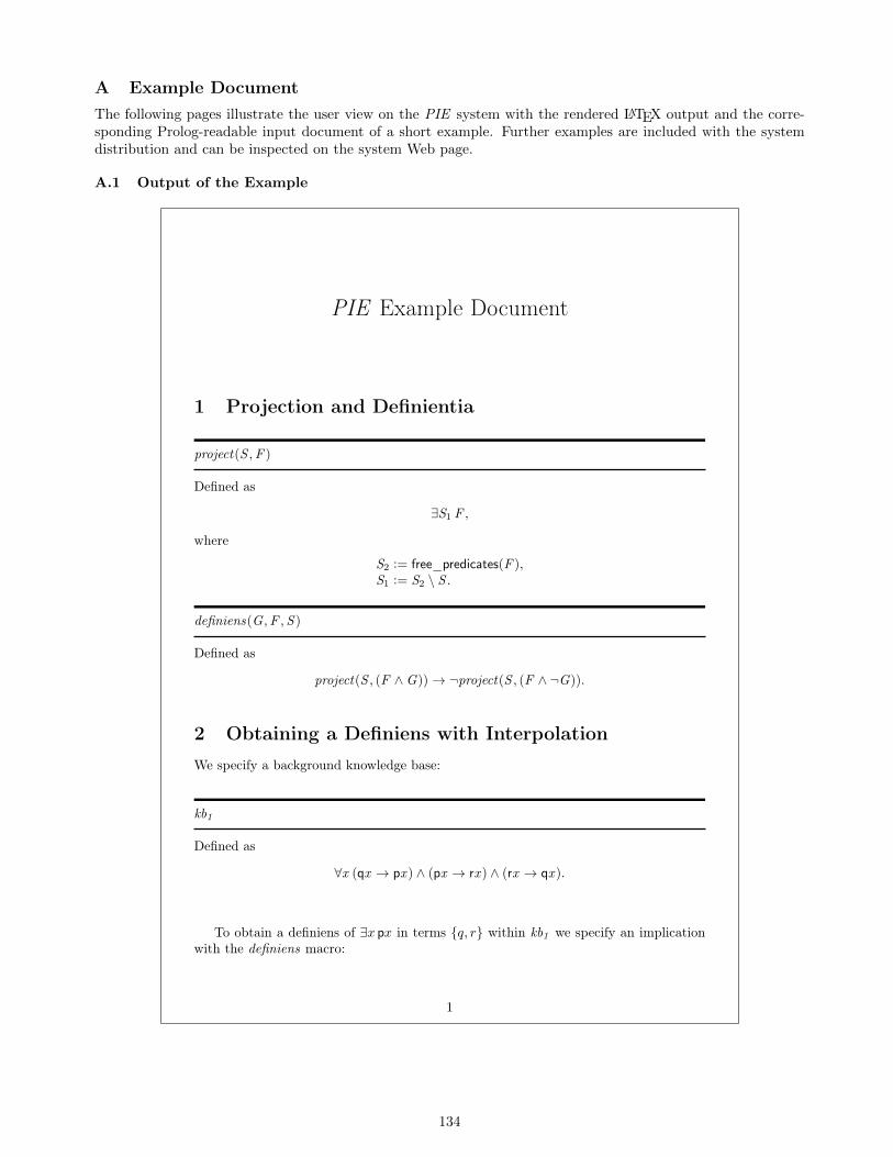
A Example Document

The following pages illustrate the user view on the PIE system with the rendered LATEX output and the corre-sponding Prolog-readable input document of a short example. Further examples are included with the systemdistribution and can be inspected on the system Web page.

A.1 Output of the Example

PIE Example Document

1 Projection and Definientia

project(S ,F )

Defined as

∃S1 F ,

where

S2 := free_predicates(F ),S1 := S2 \ S .

definiens(G ,F ,S )

Defined as

project(S , (F ∧G))→ ¬project(S , (F ∧ ¬G)).

2 Obtaining a Definiens with InterpolationWe specify a background knowledge base:

kb1

Defined as

∀x (qx → px ) ∧ (px → rx ) ∧ (rx → qx ).

To obtain a definiens of ∃x px in terms {q, r} within kb1 we specify an implicationwith the definiens macro:

1

134

ex1

Defined as

definiens((∃x px ), kb1 , [q, r]).

We now invoke a utility predicate that computes and prints for a given valid impli-cation an interpolant of its antecedent and consequent:Input: ex1 .Result of interpolation:

∃x qx .

Before we leave that example, we take a look at the expansion of ex 1:

(∃p (∀x (qx → px ) ∧ (px → rx ) ∧ (rx → qx )) ∧(∃x px )) →

¬(∃p (∀x (qx → px ) ∧ (px → rx ) ∧ (rx → qx )) ∧¬(∃x px )).

And we invoke an external prover (the E prover) to validate it:This formula is valid: ex1 .

3 Obtaining the Strongest Definiens with EliminationThe antecedent of the implication in the expansion of definiens specifies the strongestnecessary condition of G on S within F . In case definability holds (that is, the impli-cation is valid), this antecedent denotes the strongest definiens. In the example it hasa first-order equivalent that can be computed by second-order quantifier elimination.

ex2

Defined as

project([q, r], (kb1 ∧ (∃x px ))).

Input: ex2 .Result of elimination:

(∀x ¬rx ∨ qx ) ∧(∀x ¬qx ∨ rx ) ∧(∃x rx ).

2

135

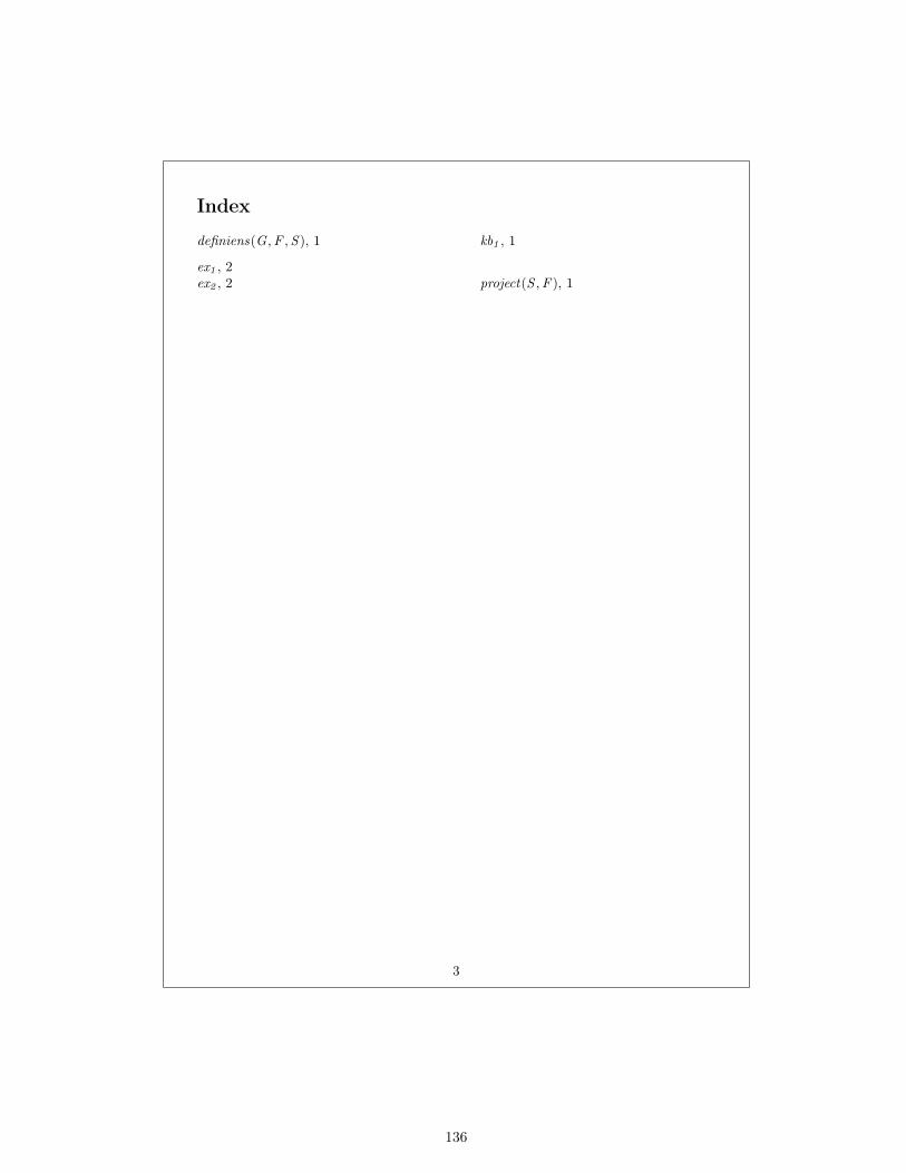
Index

definiens(G ,F ,S ), 1

ex1 , 2ex2 , 2

kb1 , 1

project(S ,F ), 1

3

136

A.2 Source of the Example

/** \title{\textit{PIE} Example Document} \date{} \maketitle */

:- use_module(folelim(support_scratch)).

:- set_info_verbosity(50).

:- ppl_set_verbosity(7).

/** \section{Projection and Definientia} */

def(project(S,F)) :: ex2(S1, F) ::-

mac_free_predicates(F, S2),

mac_subtract(S2, S, S1).

/* mac_free_predicates/2 and mac_subtract/2 are utility functions

for use in macro definitions

*/

def(definiens(G,F,S)) ::

project(S, (F , G)) -> ~project(S, (F, ~(G))).

/** \section{Obtaining a Definiens with Interpolation} */

/**

We specify a background knowledge base:

*/

def(kb_1, [syntax=brief]) ::

all(x, ((qx->px), (px->rx), (rx->qx))).

/**

\bigskip

To obtain a definiens of $\exists x\, \f{p}x$ in terms $\{q, r\}$ within

$\mathit{kb_1}$ we specify an implication with the $\mathit{definiens}$ macro:

*/

def(ex_1, [syntax=brief]) ::

definiens(ex(x, px), kb_1, [q,r]).

/**

\bigskip

We now invoke a utility predicate that computes and prints for a given valid

implication an interpolant of its antecedent and consequent:

*/

:- ppl_printtime(ppl_ipol(ex_1)).

/**

\bigskip

Before we leave that example, we take a look at the expansion of

$\mathit{ex}_1$:

*/

137

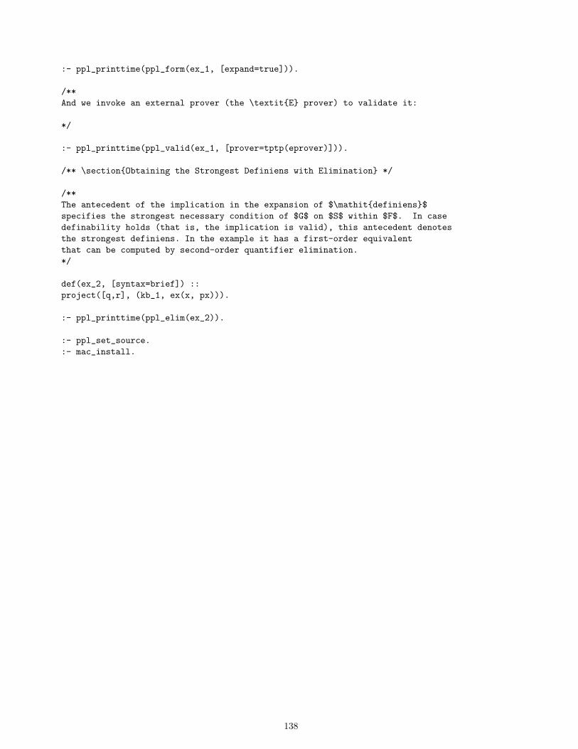
:- ppl_printtime(ppl_form(ex_1, [expand=true])).

/**

And we invoke an external prover (the \textit{E} prover) to validate it:

*/

:- ppl_printtime(ppl_valid(ex_1, [prover=tptp(eprover)])).

/** \section{Obtaining the Strongest Definiens with Elimination} */

/**

The antecedent of the implication in the expansion of $\mathit{definiens}$

specifies the strongest necessary condition of $G$ on $S$ within $F$. In case

definability holds (that is, the implication is valid), this antecedent denotes

the strongest definiens. In the example it has a first-order equivalent

that can be computed by second-order quantifier elimination.

*/

def(ex_2, [syntax=brief]) ::

project([q,r], (kb_1, ex(x, px))).

:- ppl_printtime(ppl_elim(ex_2)).

:- ppl_set_source.

:- mac_install.

138